Abstract

Building on earlier results on holographic bulk dynamics in confining gauge theories, we compute the spin-0 and spin-2 spectra of gauge theories dual to the non-singular Maldacena-Nunez and Klebanov-Strassler supergravity backgrounds. We construct and apply a numerical recipe for computing mass spectra from certain determinants. In the Klebanov-Strassler case, states containing the glueball and gluinoball obey “quadratic confinement”, i.e. their mass-squareds depend on consecutive number as $m^{2}\sim n^{2}$ for large $n$, with a universal proportionality constant. The hardwall approximation appears to work poorly when compared to the unique spectra we find in the full theory with a smooth cap-off in the infrared.

1 Introduction

One of the first successes of gauge/string duality was the computation of mass spectra of strongly coupled gauge theories from dual geometries [1, 2, 3]. These original papers were all concerned with $\mathcal{N}=0$ black hole solutions, where it is hard to check the validity of the correspondence. Other work uses the $\mathcal{N}=4$ superconformal theory (AdS bulk) plus a hard IR cut-off [4] that serves to imitate interesting field theory IR effects, but there is no running coupling. Studying $\mathcal{N}=1$ super Yang-Mills theory coupled to matter seems a good compromise in many respects: these theories exhibit confinement, chiral symmetry breaking, running couplings and a rich set of mass spectra.

For this “Non-AdS/Non-CFT correspondence”, where the bulk is not AdS and the boundary field theory is not a CFT, much less is known about mass spectra, let alone correlators. A few brave attempts exist in the literature [7, 8, 9, 10], but as we explained in [11], their results on mass spectra are at best inconclusive. In the present paper, we will compute the mass spectrum of the $\mathcal{N}=1$ Klebanov-Strassler theory [12], a non-conformal deformation of the $\mathcal{N}=1$ Klebanov-Witten theory [13] involving gluons and gluinos coupled to two sets of chiral superfields with a specific quartic superpotential. We also compute the mass spectrum of the Maldacena-Nunez background [16], as a warmup. In this way, we will be able to address physical questions about how confinement works in these models, such as whether the theory displays “linear confinement” [17].

Despite this promising state of affairs, many authors have emphasized that the aforementioned theories are still quite far from real-world QCD. For instance, there are no open strings corresponding to dynamical quarks, hence no real meson spectra. On the good side, in [18, 19], probe D-branes were added to the Klebanov-Strassler background, something which could be further developed using our methods. Real QCD is also nonsupersymmetric, and we make heavy use of the existence of a “superpotential” $W$. However, as indicated by the quotation marks, this superpotential is “fake” (in the sense of [20]), but there are nonsupersymmetric examples where such structure exists irrespective of supersymmetry per se, see e.g. [21]. Last but not least, real QCD is not at large ’t Hooft coupling $\lambda$; this is very difficult to overcome with the present state of the art, but the recent progress in [22] at least shows that $1/\sqrt{\lambda}$ corrections may not be unrealistic to obtain for these theories.

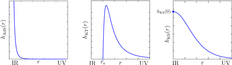
Figure 1: Warp factors $h(r)$. The string tension goes like $h^{-1/2}$. From left to right the figures show the form of the warp factor in AdS (tension goes to zero in infrared), Klebanov-Tseytlin (tension diverges at $r_{\rm s}$) and Klebanov-Strassler (tension goes to finite value).

Here, we take a step back from the effort to describe real QCD, and as mentioned above, focus on an example that is well-defined from a holographic point of view and see what can be understood about that theory. We introduce some new techniques, but conceptually the biggest difference from most of the literature is in things we do not do. We do not employ the “hard-wall” approximation (which amounts to taking AdS as in fig. 1 but with a finite IR cutoff). One argument that has been put forward to motivate the use of the hard-wall AdS model is that some physics should be insensitive to IR details. However, for computing mass spectra, a boundary condition must be imposed in the IR, so this question cannot really be insensitive to IR details (see e.g. [22]). We discuss to what extent it is in section 5.7. Another common approximation, for example in the context of inflation [23], is the singular Klebanov-Tseytlin background [24], as in fig. 1. We insist on using the full Klebanov-Strassler solution and imposing consistent boundary conditions, and find that the commonly used approximations would likely not have led to correct results even for this theory, let alone for QCD. It seems reasonable to ask for explicit computational strategies to be developed concurrently with the search for real QCD, and we believe we have made progress on such strategies here.

It is important to recall that the Klebanov-Strassler theory does not have a Wilsonian UV fixed point, but one can impose a cutoff in the UV to define the theory. One can think of this in at least three ways: 1) This is an intermediate approximation and the theory will be embedded in a more complicated theory with a UV fixed point like in [25]; 2) we will glue the noncompact dual geometry onto a compact space that naturally provides a UV cutoff like in [26]; or 3) we will want to match to (at least lattice) data at that point, and beyond that the theory is in any case not asymptotically free (for recent ideas about this, see e.g. [27]). As far as this paper is concerned, any of these points of view may be adopted.

Now to the new results in this paper. We expand upon our earlier work [11] and present a numerical strategy, the “determinant method”, to calculate the spectrum of regular and asymptotically subdominant bulk fluctuations. This puts us in the interesting position of being able to compute the mass spectrum unambiguously, but not being able to say what the composition of each mass state is without further information. This information should ideally come from data, i.e. one should compute mixings at a specified energy scale where one has some control, and use the dual theory to evolve into the deep nonperturbative regime. To illustrate this, let us take the simpler example of a theory that does have a UV fixed point. The glueball operator $\mathcal{O}_{g}$, with conformal dimension $\Delta=4$, and the gluinoball operator $\mathcal{O}_{\tilde{g}}$, with $\Delta=3$, have a diagonal mass matrix in the conformal theory. As soon as we let the theory flow away from conformality, there is a nonzero correlator $\langle\mathcal{O}_{g}\mathcal{O}_{\tilde{g}}\rangle$. We can still diagonalize at any given energy, and the mixing matrix will be energy dependent. For theories that are not conformal even in the UV, there is no preferred basis labelled by the $\Delta$ eigenvalues. One can still contemplate an approximate labelling by $\Delta$ [in the KS theory, this corresponds to expanding in the ratio $P=($number of fractional D3-branes$)/($number of regular D3-branes$)$], but it is not yet completely clear how to implement this in the dynamics; as we pointed out in [11], the limit $P\rightarrow 0$ does not commute with the UV limit one needs for the asymptotics. We will give ideas about this in sections 2.3 and 5.6, but we will not resolve it completely.

The spectra we find have some simple features. The states of the Klebanov-Strassler theory come in towers, each of which shows quadratic confinement for large excitation number (i.e. $m^{2}\sim n^{2}$, where $n$ denotes the excitation number within the tower). This confirms the claims of [17] also for the spin-0 states of the KS theory. However, for low excitation number (i.e. roughly for the first two excitations in each tower) the structure of the mass values is richer.

For the Maldacena-Nunez background, the spectrum we find is rather different. It has an upper bound, in agreement with the analytical spectra that we reported in [11].

Let us also mention that there are other approaches to holography in this type of models, such as the Kaluza-Klein holography of [28]. Some issues may appear in a different light in that framework, and that would be interesting to know.

The organization of the paper is as follows. In chapter 2 we outline the general theory of bulk fluctuations as well as the correspondence between their spectrum and the spectrum of mass states in the dual gauge theory. The presentation is done such that it is applicable also in the case of non-asymptotically AdS bulk spaces. Based on this general material, a numerical strategy to calculate the specrum will be developed in chapter 3. As a warmup, our first application will be the Maldacena-Nunez theory [16] in chapter 4, before we come to the analysis of the mass spectrum in the Klebanov-Strassler cascading gauge theory in chapter 5. Some conclusions can be found in chapter 6, and many of the more technical details have been deferred to the appendices.

2 Holographic mass spectra

We want to calculate mass spectra of confining gauge theories from the dynamics of fluctuations about their supergravity duals. In this section, we review and develop the main theoretical tools that are necessary for such a calculation. We will start, in Sec. 2.1, with a review of the treatment of the dynamics of supergravity fluctuations developed by us in [11], generalizing a similar approach to the bulk dynamics in AdS/CFT [29, 30, 31]. Then, in Sec. 2.2, we identify the bulk duals of massive states in the gauge theory as eigenfunctions of a second-order differential operator satisfying suitable boundary conditions. Most of this material belongs to AdS/CFT folklore, but we will fill in some details not commonly found in the literature. Finally, in Sec. 2.3, we will attempt to justify the identification of the gauge theory mass spectrum with the spectrum of bulk eigenfunctions by studying the pole structure of holographic two-point functions. We hope that this goes some way towards a formulation of holographic renormalization that holds beyond asymptotically AdS bulk spaces.

2.1 Linearized bulk dynamics

Let us start by reviewing the methodology we employ for studying fluctuations about bulk backgrounds that are dual to confining gauge theories. We use consistent truncations of Type IIB supergravity that describe a subsector of the 10-dimensional dynamics in terms of a 5-dimensional effective theory. Details of this trunction can be found in our earlier paper [11]. Throughout this paper, we stick to a 5-dimensional effective bulk theory, but generalization to arbitrary dimension is straightforward. The effective theory is a non-linear sigma model of scalars coupled to 5-dimensional gravity, with an action of “fake supergravity” type,

$$S=\int\,\mathrm{d}^{5}x\sqrt{g}\left[-\frac{1}{4}R+\frac{1}{2}G_{ab}(\phi)\partial_{\mu}\phi^{a}\partial^{\mu}\phi^{b}+V(\phi)\right]~{}.$$ (2.1)

The “fake supergravity” property implies that the scalar potential $V(\phi)$ follows from a superpotential $W(\phi)$ by

$$V(\phi)=\frac{1}{2}G^{ab}W_{a}W_{b}-\frac{4}{3}W^{2}~{}.$$ (2.2)

where we used the shorthand $W_{a}=\partial W/\partial\phi^{a}$.

Background solutions, also known as Poincaré-sliced domain walls or holographic renormalization group flows, are of the form

$$\begin{split}\,\mathrm{d}s^{2}&=\,\mathrm{d}r^{2}+\operatorname{e}^{2A(r)}\eta_{ij}\,\mathrm{d}x^{i}\,\mathrm{d}x^{j}~{},\\ \phi^{a}&=\bar{\phi}^{a}(r)~{},\end{split}$$ (2.3)

where the background scalars, $\bar{\phi}(r)$, and the warp function, $A(r)$, are determined by the following first-order (BPS-like) differential equations,

$$\begin{split}\partial_{r}A(r)&=-\frac{2}{3}W(\bar{\phi})~{},\\ \partial_{r}\bar{\phi}^{a}(r)&=W^{a}=G^{ab}W_{b}~{}.\end{split}$$ (2.4)

Fluctuations about the Poincaré-sliced domain wall backgrounds including the scalar and metric fields are best described gauge-invariantly. We will quote results from [11]. The physical fields are vectors in field space and scalars in spacetime, denoted by $\mathfrak{a}^{a}$, plus a traceless transverse tensor, $\mathfrak{e}^{i}_{j}$, where $i,j=1,2,3,4$ are the indices along 4-dimensional Poincaré slices. These fields satisfy the following linearized field equations,

$$\left[\left(\delta^{a}_{b}D_{r}+W^{a}_{\;\;|b}-\frac{W^{a}W_{b}}{W}-\frac{8}{3}W\delta^{a}_{b}\right)\left(\delta^{b}_{c}D_{r}-W^{b}_{\;\;|c}+\frac{W^{b}W_{c}}{W}\right)+\delta^{a}_{c}\operatorname{e}^{-2A}\Box\right]\mathfrak{a}^{c}=0~{},$$ (2.5)

and

$$\left(\partial_{r}^{2}-\frac{8}{3}W\partial_{r}+\operatorname{e}^{-2A}\Box\right)\mathfrak{e}^{i}_{j}=0~{}.$$ (2.6)

In (2.5) and (2.6), $\Box=\eta^{ij}\partial_{i}\partial_{j}$, which will be replaced by $-k^{2}$ when we work in 4-dimensional momentum space. Also, we use a sigma-model covariant notation, lowering and raising indices of sigma-model tensors with $G_{ab}$ and its inverse $G^{ab}$, and a sigma-model covariant derivative $D_{a}$ that acts as

$$D_{a}\varphi_{b}\equiv\varphi_{a|b}\equiv\partial_{b}\varphi_{a}-\mathcal{G}^{c}_{\;\;ab}\varphi_{c}~{},$$ (2.7)

where $\mathcal{G}^{c}_{\;\;ab}$ is the Christoffel symbol derived from the metric $G_{ab}$. Furthermore, we define a “background-covariant” derivative $D_{r}$ ($r$ is the radial coordinate of (2.3)) acting as

$$D_{r}\varphi^{a}=\partial_{r}\varphi^{a}+\mathcal{G}^{a}_{\;\;bc}W^{b}\varphi^{c}~{}.$$ (2.8)

So, our task is to solve (2.5) and (2.6) for the backgrounds of interest, imposing appropriate boundary conditions that we now describe.

2.2 Bulk duals of mass states

In AdS/CFT, the usual definition of the bulk dual of a boundary gauge theory mass state is a solution of the (linearized) bulk field equations that is regular and integrable. In the following, we will state these notions more precisely and present them in a form that is suitable also for application in non-AdS/non-CFT.

As prototype for the equations of motion (2.5) and (2.6), we consider a system of $n$ coupled second-order differential equations of the generic form

$$\left[D_{r}^{2}-\frac{8}{3}WD_{r}+M(r)-\operatorname{e}^{-2A(r)}k^{2}\right]\mathfrak{a}=0~{},$$ (2.9)

where $D_{r}$ is the background-covariant derivative (2.7), $M$ is a symmetric field-space tensor ($M_{ab}=M_{ba}$), and field indices have been omitted for the sake of brevity. We also assume that the radial coordinate $r$ is defined in a domain $r_{\text{IR}}\leq r<\infty$, where $r\approx r_{\text{IR}}$ corresponds to the deep interior (IR) region, and large $r$ to the asymptotic (UV) region of the bulk.

Let us start with the regularity condition. As we want the 10-dimensional configuration obtained via uplifting of an effective 5-dimensional solution to be singularity-free, we must impose that also the 5-d solutions be regular in the bulk. For nonsingular backgrounds, (2.9) typically has a regular singular point at $r_{\text{IR}}$ and no others for finite $r$. Regularity in the bulk, therefore, means regularity at $r_{\text{IR}}$. To make sure that our regularity condition is invariant under changes of field space variables, we require that the norm of the fluctuation vector is finite at $r=r_{\text{IR}}$,

$$\text{\emph{Regularity condition:}}\qquad\left(\mathfrak{a}^{a}G_{ab}\,\mathfrak{a}^{b}\right)_{r=r_{\text{IR}}}<\infty~{}.$$ (2.10)

We emphasize that one cannot simply demand regularity of the components of $\mathfrak{a}^{a}$ at $r=r_{\text{IR}}$, because $r=r_{\text{IR}}$ can coincide with a coordinate singularity in the sigma-model metric $G_{ab}$, when evaluated on the background. In the examples we consider, this indeed happens.

From the $2n$ independent solutions of (2.9), the condition (2.10) typically selects precisely $n$ independent regular solutions, which we will denote by $\mathfrak{a}_{\mathrm{reg}}{}_{,i}$, and $n$ singular solutions, denoted by $\mathfrak{a}_{\mathrm{sing}}{}_{,i}$. A generic solution of (2.9) is a linear combination of these,

$$\mathfrak{a}(r)=c_{i}\,\mathfrak{a}_{\mathrm{reg}}{}_{,i}(r)+\tilde{c}_{i}\,\mathfrak{a}_{\mathrm{sing}}{}_{,i}(r)$$ (2.11)

with constants $c_{i}$ and $\tilde{c}_{i}$. Thus, (2.10) implies that

$$\tilde{c}_{i}=0\qquad\text{for all $i$.}$$ (2.12)

Now, consider the integrability condition. Let us take a small detour and consider the bulk Green’s function $G(r,r^{\prime};k^{2})$, which satisfies

$$\left[D_{r}^{2}-\frac{8}{3}WD_{r}+M(r)-\operatorname{e}^{-2A(r)}k^{2}\right]G(r,r^{\prime};k^{2})=-\operatorname{e}^{-4A(r)}\delta(r-r^{\prime})~{},$$ (2.13)

where the factor $\operatorname{e}^{-4A}$ on the right hand side is the metric factor $1/\sqrt{g}$ from the covariant delta functional. The Green’s function can be written in terms of a basis of eigenfunctions,

$$G(r,r^{\prime},k^{2})=\sum\limits_{\lambda}\frac{\mathfrak{a}_{\lambda}(r)\mathfrak{a}_{\lambda}(r^{\prime})}{k^{2}+m_{\lambda}^{2}}~{},$$ (2.14)

where the functions $\mathfrak{a}_{\lambda}$ satisfy (2.9) for $k^{2}=-m_{\lambda}^{2}$.(Again, we omit the matrix indices, and the indices of the two $\mathfrak{a}_{\lambda}$’s are not contracted.) Substituting (2.14) into (2.13) yields the completeness relation

$$\sum\limits_{\lambda}\mathfrak{a}_{\lambda}(r)\mathfrak{a}_{\lambda}(r^{\prime})=\operatorname{e}^{-2A(r)}\delta(r-r^{\prime})~{},$$ (2.15)

from which one can deduce the orthogonality relation

$$\int\,\mathrm{d}r\,\operatorname{e}^{2A(r)}\mathfrak{a}_{\lambda}(r)\cdot\mathfrak{a}_{\sigma}(r)=\delta_{\lambda\sigma}~{}.$$ (2.16)

With the dot product we denote the covariant contraction of indices. Eq. (2.16) provides the condition for the eigenstates $\mathfrak{a}_{\lambda}$ to be integrable. Due to the factor $\operatorname{e}^{2A}$ (for general dimension $d$ it would be $\operatorname{e}^{(d-2)A}$), the integral measure is not the covariant bulk integral measure that one might have expected.

Now, the spectrum of bulk eigenfunctions $\mathfrak{a}_{\lambda}$ is identified with the mass spectrum of operators dual to the fields $\mathfrak{a}$. (We will also say that the eigenfunction $\mathfrak{a}_{\lambda}$ is the bulk dual of a state of mass $m_{\lambda}$.) Clearly, this spectrum depends on the boundary conditions one imposes. One boundary condition is given by the regularity condition (2.10), the other follows from (2.16), namely

$$\text{\emph{Integrability condition:}}\qquad\int\,\mathrm{d}r\,\operatorname{e}^{2A(r)}\mathfrak{a}(r)\cdot\mathfrak{a}(r)<\infty~{}.$$ (2.17)

For large $r$, i.e., in the UV, (2.9) has $2n$ independent asymptotic solutions. Let us denote the $n$ dominant ones by $\mathfrak{a}_{\mathrm{dom}}{}_{,i}$, and the $n$ subdominant ones by $\mathfrak{a}_{\mathrm{sub}}{}_{,i}$ (by “dominant” we mean leading in $r$). Again, a generic solution of (2.9) can be written as a linear combination of these,

$$\mathfrak{a}(r)=d_{i}\,\mathfrak{a}_{\mathrm{sub}}{}_{,i}(r)+\tilde{d}_{i}\,\mathfrak{a}_{\mathrm{dom}}{}_{,i}(r)\,\;,$$ (2.18)

with constants $d_{i}$ and $\tilde{d}_{i}$.

It can be checked in the various cases we consider that the asymptotically dominant behaviours, $\mathfrak{a}_{\mathrm{dom}}{}_{,i}$, are not integrable in the sense of (2.17), whereas the subdominant behaviours are integrable. Thus, (2.17) is equivalent to

$$\tilde{d}_{i}=0\qquad\text{for all $i$.}$$ (2.19)

To summarize, the eigenfunctions $\mathfrak{a}_{\lambda}$, interpreted as the bulk duals of boundary field theory states with mass $m_{\lambda}$, are such that

$$\tilde{c}_{i}=\tilde{d}_{i}=0\qquad\text{$i=1,2,\ldots n$,}$$ (2.20)

from which follows that

$$\mathfrak{a}_{\lambda}(r)=c_{\lambda,i}\,\mathfrak{a}_{\mathrm{reg}}{}_{,i}(r)=d_{\lambda,i}\,\mathfrak{a}_{\mathrm{sub}}{}_{,i}(r)~{}.$$ (2.21)

2.3 Pole structure of holographic 2-point functions

The masses of states (particles) in a quantum field theory manifest themselves as poles in the two-point functions of operators, if there is a non-zero probability that these states are created by the operators from the vacuum,

$$\int\,\mathrm{d}^{4}x\,\operatorname{e}^{ikx}\left\langle{\mathcal{O}_{1}(x)\mathcal{O}_{2}(0)}\right\rangle=\sum\limits_{\lambda}\frac{\langle{0}|\mathcal{O}_{1}(0)|{\lambda}\rangle\langle{\lambda}|\mathcal{O}_{2}(0)|{0}\rangle}{k^{2}+m_{\lambda}^{2}}+\text{c.t.}\ .$$ (2.22)

For comparison with this general formula, we will now try to obtain the pole structure of holographic 2-point functions from the linearized dynamics of the bulk fields that we described in Sec. 2.1. But we must start with a disclaimer. As we have not systematically dealt with the renormalization and dictionary problems (see the discussion in [11]), our results will depend on two strong assumptions, motivated by how things work in AdS/CFT. A better understanding of these assumptions as well as the meaning of cases in which they are not satisfied would be very desirable.

Let us start with the asymptotic expansion of the bulk fields (2.18). For a given bulk field $\mathfrak{a}$, the coefficients $d_{i}$ and $\tilde{d}_{i}$ clearly depend on the choice of basis functions $\mathfrak{a}_{\mathrm{sub}}{}_{,i}$ and $\mathfrak{a}_{\mathrm{dom}}{}_{,i}$, respectively. In order to remove some of the ambiguities, we assume that the term containing $k^{2}$ in the equation of motion (2.9) is asymptotically suppressed, so that the leading terms of the asymptotic solutions are independent of $k^{2}$, and the subleading terms can depend only on powers of $k^{2}$ (assumption 1). Then, we can choose a basis of asymptotic solutions such that each has a distinct leading behaviour. These solutions are classified according to their asymptotic growth with the radial coordinate into dominant and subdominant solutions. With each dominant asymptotic solution $\mathfrak{a}_{\mathrm{dom}}{}_{,i}$, we associate an operator $\mathcal{O}_{i}$ of the dual field theory. Two ambiguities still remain in the choice of basis functions, but we now argue that these correspond to field theory ambiguities. First, the normalization of the leading terms in the asymptotic basis solutions can be freely chosen. In field theory this corresponds to a choice of normalization of the operators $\mathcal{O}_{i}$, which always drops out in physical scattering amplitudes. Second, we have the freedom to add to a given dominant solution multiples of asymptotic solutions of equal or weaker strength, with coefficients polynomial in $k^{2}$. (Solutions of equal strength can be added only with coefficients independent of $k^{2}$.) This is also expected from the dual field theory, since operators of a given dimension can mix with operators of equal or lower dimensions (higher dimension operators being suppressed by our large UV cutoff) which implies that generically, there is no unique way to define the renormalized operators. Therefore, the remaining ambiguities in the choice of an asymptotic basis of solutions reflect the usual freedom in the definition of field theory operators.

For what follows, we do not need to make particular choices for the subdominant basis solutions, $\mathfrak{a}_{\mathrm{sub}}{}_{,i}$. This will be clearer once we obtain our final result of this section, i.e. (2.34).

Now for the second assumption. In a field theory calculation of correlation functions of the operators $\mathcal{O}_{i}$, one adds a source term to the Lagrangian,

$$\Delta\mathcal{L}=-\tilde{d}_{i}\mathcal{O}_{i}~{}.$$ (2.23)

In holography, the sources are identified with the coefficients $\tilde{d}_{i}$ of (2.18), whose dependence on $k^{2}$ was suppressed in that equation. The second strong assumption we make is the generic form of the exact one-point function of the operators $\mathcal{O}_{i}$. In AdS/CFT, the response functions $d_{i}$ of (2.18) encode the exact one-point functions, up to scheme dependent terms that are local in the sources [34, 35, 36, 37]. In view of the ambiguities discussed above, we assume

$$\left\langle{\mathcal{O}_{i}(k)}\right\rangle_{\text{exact}}=Y_{ij}(k^{2})\,d_{j}(k^{2})+\text{local terms}~{},$$ (2.24)

with a matrix $Y_{ij}(k^{2})$, which we will be able to determine further below (assumption 2). Part of the assumption is that the poles of the connected 2-point functions arise in $d_{j}$, and that $Y_{ij}$ does not give rise to additional poles. In AdS/CFT, (2.24) follows from holographic renormalization, but unfortunately we have no proof of it in this more general setting.

We will now derive the general pole structure of holographic 2-point functions. To start, consider the general formula for a solution $\mathfrak{a}(r,k^{2})$ of (2.9) in terms of the Green’s function and prescribed boundary values. Let $r_{0}$ be a (large) cut-off parameter determining the hypersurface where the boundary values are formally prescribed. Remembering that neither the Green’s function nor its derivative vanish at the cut-off boundary, we have

$$\mathfrak{a}(r,k^{2})=\operatorname{e}^{4A(r_{0})}\left[(D_{r_{0}}\mathfrak{a}(r_{0},k^{2}))\cdot G(r_{0},r;k^{2})-\mathfrak{a}(r_{0},k^{2})\cdot D_{r_{0}}G(r_{0},r;k^{2})\right]~{},$$ (2.25)

where $\mathfrak{a}(r_{0},k^{2})$ and $D_{r_{0}}\mathfrak{a}(r_{0},k^{2})$ are the prescribed values of the field and its first derivative at the cut-off boundary, respectively. Since $r_{0}$ is an unphysical cut-off parameter, we must ensure that the bulk field $\mathfrak{a}(r)$ remains unchanged when $r_{0}$ is varied. This is easily achieved, if, together with a change of the cut-off, $r_{0}\to r_{0}+\delta r_{0}$, the boundary values are changed by

$$\delta\mathfrak{a}(r_{0},k^{2})=(D_{r_{0}}\mathfrak{a}(r_{0},k^{2}))\,\delta r_{0}~{},\qquad\delta D_{r_{0}}\mathfrak{a}(r_{0},k^{2})=(D^{2}_{r_{0}}\mathfrak{a}(r_{0},k^{2}))\,\delta r_{0}~{},$$ (2.26)

and the second derivative, $D^{2}_{r_{0}}\mathfrak{a}(r_{0},k^{2})$, is determined by the equation of motion (2.9). To assure (2.26), we determine the formal boundary values at the cut-off, $\mathfrak{a}(r_{0},k^{2})$ and $D_{r_{0}}\mathfrak{a}(r_{0},k^{2})$, from the generic asymptotic behaviour (2.18), with coefficients $d_{i}$ and $\tilde{d}_{i}$ fixed. After inserting (2.18) and (2.14) into (2.25), we obtain

$$\begin{split}\mathfrak{a}(r,k^{2})&=\operatorname{e}^{4A(r_{0})}\sum\limits_{\lambda}\frac{\mathfrak{a}_{\lambda}(r)}{k^{2}+m_{\lambda}^{2}}\times\\ &\quad\times\left\{d_{l}\left[(D_{r_{0}}\mathfrak{a}_{\mathrm{sub}}{}_{,l}(r_{0},k^{2}))\cdot\mathfrak{a}_{\lambda}(r_{0})-\mathfrak{a}_{\mathrm{sub}}{}_{,l}(r_{0},k^{2})\cdot D_{r_{0}}\mathfrak{a}_{\lambda}(r_{0})\right]+\right.\\ &\quad\quad+\tilde{d}_{l}\left.\left[(D_{r_{0}}\mathfrak{a}_{\mathrm{dom}}{}_{,l}(r_{0},k^{2}))\cdot\mathfrak{a}_{\lambda}(r_{0})-\mathfrak{a}_{\mathrm{dom}}{}_{,l}(r_{0},k^{2})\cdot D_{r_{0}}\mathfrak{a}_{\lambda}(r_{0})\right]\right\}~{}.\end{split}$$ (2.27)

To continue, we observe that for very large $r_{0}$, the term on the second line of (2.27), containing only subdominant solutions, is much smaller than the term on the third line. Therefore, we drop it. Moreover, as we are interested only in the pole structure, we consider $k^{2}$ very close to $-m_{\lambda}^{2}$ and expand the numerator keeping only the leading term, i.e., we replace $k^{2}$ by $-m_{\lambda}^{2}$ in the numerator. Finally, we use the fact that the eigenfunctions are purely subdominant,

$$\mathfrak{a}_{\lambda}(r)=d_{\lambda,i}\,\mathfrak{a}_{\mathrm{sub}}{}_{,i}(r,-m_{\lambda}^{2})~{}.$$ (2.28)

This yields

$$\mathfrak{a}(r,k^{2})\underset{k^{2}\approx-m_{\lambda}^{2}}{=}\tilde{d}_{l}\,Z_{lj}(-m_{\lambda}^{2})\,\frac{d_{\lambda,j}d_{\lambda,i}}{k^{2}+m_{\lambda}^{2}}\;\mathfrak{a}_{\mathrm{sub}}{}_{,i}(r,-m_{\lambda}^{2})~{},$$ (2.29)

with

$$Z_{ij}(k^{2})=\operatorname{e}^{4A(r)}\left[(D_{r}\mathfrak{a}_{\mathrm{dom}}{}_{,i}(r,k^{2}))\cdot\mathfrak{a}_{\mathrm{sub}}{}_{,j}(r,k^{2})-\mathfrak{a}_{\mathrm{dom}}{}_{,i}(r,k^{2})\cdot D_{r}\mathfrak{a}_{\mathrm{sub}}{}_{,j}(r,k^{2})\right]~{}.$$ (2.30)

Notice that, by virtue of the equation of motion (2.9), $Z_{ij}$ is independent of $r$.

Thus, after reading off the response function $d_{i}$ from (2.29), we obtain the poles of the connected 2-point function, using (2.24) and differentiating with respect to the source $\tilde{d}_{j}$,

$$\left\langle{\mathcal{O}_{i}(k)\mathcal{O}_{j}(-k)}\right\rangle=\sum\limits_{\lambda}Y_{ii^{\prime}}(-m_{\lambda}^{2})Z_{jj^{\prime}}(-m_{\lambda}^{2})\,\frac{d_{\lambda,i^{\prime}}d_{\lambda,j^{\prime}}}{k^{2}+m_{\lambda}^{2}}+\text{c.t.}\ .$$ (2.31)

By symmetry, we find that $Y_{ij}$ equals $Z_{ij}$ up to normalization,

$$Y_{ij}(-m_{\lambda}^{2})=N_{\lambda}Z_{ij}(-m_{\lambda}^{2})~{}.$$ (2.32)

Therefore, defining also

$$Z_{\lambda,i} =Z_{ii^{\prime}}(-m_{\lambda}^{2})\,d_{\lambda,i^{\prime}}$$

$$=\operatorname{e}^{4A(r)}\left[(D_{r}\mathfrak{a}_{\mathrm{dom}}{}_{,i}(r,-m_{\lambda}^{2}))\cdot\mathfrak{a}_{\lambda}(r)-\mathfrak{a}_{\mathrm{dom}}{}_{,i}(r,-m_{\lambda}^{2})\cdot D_{r}\mathfrak{a}_{\lambda}(r)\right]~{},$$ (2.33)

our final result is

$$\left\langle{\mathcal{O}_{i}(k)\mathcal{O}_{j}(-k)}\right\rangle=\sum\limits_{\lambda}N_{\lambda}\frac{Z_{\lambda,i}Z_{\lambda,j}}{k^{2}+m_{\lambda}^{2}}+\text{c.t.}\ .$$ (2.34)

We note that the $Z_{\lambda,i}$ are independent of the choice of the subdominant basis solutions, because the normalization of the eigenfunctions $\mathfrak{a}_{\lambda}$ is fixed by (2.16).

The determination of the normalization factors $N_{\lambda}$ is an open problem, whose solution is intimately related with finding a proof of (2.24). We conjecture that $N_{\lambda}=1$, as can be easily checked for asymptotic AdS bulk spaces (see Appendix A).

3 Finding Mass States

In the previous section, we characterized the duals of mass states as regular (in the IR) and asymptotically subdominant (in the UV) solutions of the linearized bulk field equations. To calculate the spectrum, one solves a system of second-order differential equations with boundary conditions specified at two endpoints. The standard numerical strategy for this is “shooting”, in which one solves the corresponding initial value problem with two boundary conditions (field value and derivative) specified at the initial point, and then varies the initial condition trying to find the desired boundary value at the final point. For coupled multifield systems, this is a laborious process. Fortunately, since we are interested only in the spectrum and not in the explicit dual bulk solutions, we can adopt a much simpler strategy. It involves computing a single function, the determinant of a matrix, that depends on the momentum $k^{2}$ and the vanishing of which signals the presence of a mass state.

In Sec. 3.1, we shall present the general idea of our strategy in its simplest implementation involving the numerical solution of the field equations as an initial value problem starting close to $r_{\text{IR}}$. This simple implementation presents some numerical challenges, which we describe, and which are overcome with the refined method described in Sec. 3.2. Further details of numerical issues will be deferred to Appendix E.

3.1 Mass Spectrum: Determinant Method

We begin by imposing regularity in the IR. This means that we consider the equations of motion for $r\approx r_{\text{IR}}$, find independent solutions of these, and impose $\tilde{c}_{i}=0$ in the language of Sec. 2.2. Starting with these initial conditions, one numerically evolves to larger $r$ to obtain the $n$ regular bulk solutions $\mathfrak{a}_{\mathrm{reg}}{}_{,i}(r)$. For large $r$, the asymptotic behavior of each of these solution can be expanded in terms of the UV-dominant solutions $\mathfrak{a}_{\mathrm{dom}}{}_{,j}$, so that

$$\mathfrak{a}_{\mathrm{reg}}{}_{,i}(r)\approx\gamma_{ji}\,\mathfrak{a}_{\mathrm{dom}}{}_{,j}(r)\qquad\text{(large $r$)}~{},$$ (3.1)

for some $k^{2}$-dependent but $r$-independent constants $\gamma_{ji}$. (The order of indices has been chosen for later convenience. As a reminder, both $\mathfrak{a}_{\mathrm{reg}}{}_{,i}(r)$ and $\mathfrak{a}_{\mathrm{dom}}{}_{,j}(r)$ are $n$-component vectors in field space, but we are suppressing the field-space index.) Thus, a general regular solution (cf. (2.11)) will behave as

$$\mathfrak{a}_{\mathrm{reg}}{}(r)\approx c_{i}\gamma_{ji}\,\mathfrak{a}_{\mathrm{dom}}{}_{,j}(r)\qquad\text{(large $r$)}~{}.$$ (3.2)

In order for $\mathfrak{a}_{\mathrm{reg}}{}$ to qualify as the bulk dual of a boundary field theory mass eigenstate, the remaining condition in (2.20) is $\tilde{d}_{i}=0$ for the fluctuation to be integrable. Thus,

$$\tilde{d}_{i}=\gamma_{ij}c_{j}=0\quad\text{for all $i$}\quad\Longleftrightarrow\quad\text{mass state}~{}.$$ (3.3)

Regarding this as a set of $n$ equations for the coefficients $c_{i}$, it is necessary and sufficient for the existence of non-zero solutions that the determinant of the matrix $\gamma_{ij}$ be zero:

$$\det\gamma_{ij}(k^{2})=0\quad\Longleftrightarrow\quad\text{mass state with $m^{2}=-k^{2}$}~{},$$ (3.4)

where we have restored the dependence of the matrix $\gamma_{ij}$ on the 4-momentum $k^{2}$.

To compute $\gamma_{ij}$, let us make the field-space component index explicit in eq. (3.1):

$$(\mathfrak{a}_{\mathrm{reg}}{}(z))_{~{}i}^{a}\approx\gamma_{ji}(\mathfrak{a}_{\mathrm{dom}}{}(z))_{~{}j}^{a}$$ (3.5)

where $\mathfrak{a}_{\mathrm{reg}}{}(z)$ and $\mathfrak{a}_{\mathrm{dom}}{}(z)$ are viewed as $n\times n$ matrices, with column index $i$ and row index $a$. Inverting this equation, the coefficient matrix $\gamma_{ij}$ can be found by calculating

$$\gamma_{ij}\approx\left[(\mathfrak{a}_{\mathrm{dom}}{})^{-1}(\mathfrak{a}_{\mathrm{reg}}{})\right]_{ij}$$ (3.6)

for some large value of $r$, where the subdominant parts of $\mathfrak{a}_{\mathrm{reg}}{}$ are sufficiently suppressed. We would like to emphasize that formula (3.6) renders the coefficients $\gamma_{ij}$ independent of the coordinates in field space — the component index $a$ is contracted. Hence, also the mass condition (3.4) is independent of the choice of sigma-model variables.

However, as announced above, the IR $\rightarrow$ UV determinant method does not work straightforwardly for coupled multifield systems in practice. The method is only sufficiently insensitive to numerical error if all dominant solutions $\mathfrak{a}_{\mathrm{dom}}{}_{,i}$ are comparable in magnitude, such that the integration error from the stronger ones does not swamp the significant digits of the weaker ones. For 1-component systems, this is obviously never a problem, and it turns out also not to be a problem for the 2-component system in the MN background (Section 4.3). In general, and in particular for the 7-component spin-0 system in the KS background, it is better to tread more carefully and only evolve to a prescribed midpoint value, as we will describe in the next subsection.

One could have imagined that this numerical difficulty would be alleviated by evolving the other way (UV $\rightarrow$ IR). This is actually partially true, but the method in the next subsection is still more useful (see Appendix E for a few more details). Indeed, imposing the relevant initial conditions at a large value of $r$, one can calculate numerically the $n$ UV-subdominant solutions $\mathfrak{a}_{\mathrm{sub}}{}_{,i}$. Decomposing their behavior at $r\approx r_{\text{IR}}$ using (2.11) into

$$\mathfrak{a}_{\mathrm{sub}}{}_{,i}(r)=\gamma_{ji}\,\mathfrak{a}_{\mathrm{sing}}{}_{,j}(r)+{\gamma^{\prime}}_{ji}\,\mathfrak{a}_{\mathrm{reg}}{}_{,j}(r)~{},$$ (3.7)

the same argument as before affirms that an $\mathfrak{a}_{\mathrm{sub}}{}$ dual to a mass eigenstate exists, if $\det\gamma_{ij}=0$. The coefficients $\gamma_{ij}$ can be determined by matching the components of $\mathfrak{a}_{\mathrm{sub}}{}$ to the generic singular behaviour.

The build-up and growth of integration error on the way from the asymptotic region to $r_{\text{IR}}$ is an issue here and must be resolved. This can be done by making sure the UV cutoff is not too large. Then, the integration error, which generally grows like the asymptotically weakest solution, remains small.

3.2 Mass Spectrum: Midpoint Determinant Method

The midpoint method is numerically the most stable and combines the two previous approaches. One calculates the asymptotic solutions analytically both in the UV and in the IR. Then, the $n$ regular solutions $\mathfrak{a}_{\mathrm{reg}}{}_{,i}$ are evolved from $r\approx r_{\text{IR}}$ up to a mid-point $r_{\text{mid}}$, and the $n$ subdominant solutions $\mathfrak{a}_{\mathrm{sub}}{}_{,i}$ are evolved from large $r$ down to $r_{\text{mid}}$. Then, one tries to find linear combinations of the regular solutions and of the subdominant solutions, respectively, such that their value and first derivative at $r_{\text{mid}}$ match:

$$\begin{pmatrix}\mathfrak{a}_{\mathrm{reg}}{}&\mathfrak{a}_{\mathrm{sub}}{}\\ \partial_{r}\mathfrak{a}_{\mathrm{reg}}{}&\partial_{r}\mathfrak{a}_{\mathrm{sub}}{}\end{pmatrix}_{\!\!r=r_{\text{mid}}}\begin{pmatrix}c\\ -d\end{pmatrix}=0~{}.$$ (3.8)

As before, the necessary and sufficient condition for the existence of a mass eigenstate is given by the determinant of a matrix (this time $2n\times 2n$) being zero. Put differently, rather than demanding that a given individual field match smoothly across the midpoint, we allow for the situation that only some linear combination of the basis fields matches smoothly, and this linear combination is determined by the coefficients $c$ and $d$.

If the solutions we are matching were approximate analytical solutions and the midpoint were the classical turning point, this midpoint matching would be precisely the WKB approximation. Of course, our solutions will not be approximate analytical, but numerical and exact (up to integration error), so it is no approximation in that sense.

4 Maldacena-Nunez system

4.1 General Relations

The effective 5-d model describing the bulk dynamics of the MN system contains three scalar fields $(g,a,p)$ and is characterized by the sigma-model metric [38, 11]

$$G_{ab}\partial_{\mu}\phi^{a}\partial^{\mu}\phi^{b}=\partial_{\mu}g\partial^{\mu}g+\operatorname{e}^{-2g}\partial_{\mu}a\partial^{\mu}a+24\partial_{\mu}p\partial^{\mu}p~{},$$ (4.1)

and the superpotential

$$W=-\frac{1}{2}\operatorname{e}^{4p}\left[(a^{2}-1)^{2}\operatorname{e}^{-4g}+2(a^{2}+1)\operatorname{e}^{-2g}+1\right]^{1/2}~{}.$$ (4.2)

Let us summarize what Poincaré-sliced domain wall backgrounds this system admits. In what follows, we shall denote the background values of the scalar fields by $g$, $a$ and $p$, and for their fluctuations we will use the gauge-invariant sigma-model vector $\mathfrak{a}=(\delta g,\delta a,\delta p)^{T}$. The background equations (2.4) are most easily solved in terms of a new radial coordinate, $\rho$, defined by

$$\partial_{\rho}=2\operatorname{e}^{-4p}\partial_{r}~{}.$$ (4.3)

We shall need only the explicit solutions for $a$ and $g$, which are given by

$$a=\frac{2\rho}{\sinh(2\rho+c)}~{},\quad\operatorname{e}^{2g}=4\rho\coth(2\rho+c)-(a^{2}+1)~{}.$$ (4.4)

The integration constant $c$, which appeared for the first time in [39], can take values $0\leq c\leq\infty$. The regular MN solution corresponds to $c=0$, while $c>0$ leads to singular bulk geometries. The solution (4.4) is defined for $\rho\geq\hat{\rho}$, with $\hat{\rho}$ defined by $\operatorname{e}^{2g(\hat{\rho})}=0$, from which one obtains the relation

$$\coth(2\hat{\rho}+c)=\frac{1}{2\hat{\rho}}-1~{}.$$ (4.5)

Hence, $\hat{\rho}$ takes values between $0$ and $1/4$, with $\hat{\rho}=0$ for $c=0$ and $\hat{\rho}=1/4$ for $c=\infty$. For $c>0$, $\rho=\hat{\rho}$ is the location of the singularity.

For the scalar $p$ we will only need its relation to the warp function $A$ (see (2.3)), which is

$$\operatorname{e}^{-2A}\operatorname{e}^{-8p}=C^{2}~{},$$ (4.6)

where $C^{2}$ is an integration constant setting the 4-d scale. For later convenience, we set $C^{2}=1/4$.

Let us turn to the fluctuation equations (2.5) and (2.6) in terms of the radial variable $\rho$. After using the relations for the background, one straightforwardly finds that (2.5) becomes

$$\left[(\partial_{\rho}-M)(\partial_{\rho}-N)-k^{2}\right]\mathfrak{a}=0~{},$$ (4.7)

where we dropped field indices, and the matrices $M$ and $N$ are given by

$$\begin{split}N^{a}_{~{}b}&=2\operatorname{e}^{-4p}\left(\partial_{b}W^{a}-\frac{W^{a}W_{b}}{W}\right)~{},\\ M^{a}_{~{}b}&=-N^{a}_{~{}b}-4\operatorname{e}^{-4p}\left(\mathcal{G}^{a}_{\;\;bc}W^{c}-W\delta^{a}_{b}\right)~{}.\end{split}$$ (4.8)

Note that $M$ and $N$ are independent of $p$. As was observed in [11], the fluctuations of $p$, which are described by the component $\mathfrak{a}^{3}$, decouple from the other two. This can be seen from (4.8) as follows. From (4.1) and (4.2) we find the identities

$$W_{3}=4W~{},\qquad W^{3}=\frac{1}{6}W~{},\qquad\partial_{p}W^{a}=4W^{a}~{},$$ (4.9)

from which follow $N^{a}_{~{}3}=N^{3}_{~{}b}=0$. Moreover, one easily checks that $\mathcal{G}^{3}_{\;\;bc}=\mathcal{G}^{a}_{\;\;3c}=0$, so that $M^{a}_{~{}3}=4\operatorname{e}^{-4p}W\delta^{a}_{3}$, and $M^{3}_{~{}b}=4\operatorname{e}^{-4p}W\delta^{3}_{b}$. Thus, $\mathfrak{a}^{3}$ satisfies

$$\left[(\partial_{\rho}-4\operatorname{e}^{-4p}W)\partial_{\rho}-k^{2}\right]\mathfrak{a}^{3}=0~{}.$$ (4.10)

This is just the equation for a massless scalar field in the domain wall background.

Similarly, (2.6) gives rise to

$$\left[(\partial_{\rho}-4\operatorname{e}^{-4p}W)\partial_{\rho}-k^{2}\right]\mathfrak{e}^{i}_{j}=0~{}.$$ (4.11)

which is identical to (4.10).

4.2 Analytic solutions in singular background

We will briefly introduce the analytical solutions for the fluctuations in the singular background case $c=\infty$ derived in [11]. These analytical solutions give useful indications for glueball and gluinoball masses that can be compared with the numerical analysis in Sec. 4.3. Further details can be found in our earlier paper [11].

Let us start with (4.7). In the case $c=\infty$, the matrices $M$ and $N$ are very simple and diagonal,

$$\begin{split}M&=\frac{1}{4\rho-1}\operatorname{diag}\left(-8\rho+4-\frac{1}{\rho},-2+\frac{1}{\rho},-8\rho\right)~{},\\ N&=\operatorname{diag}\left(-\frac{1}{\rho},\frac{1}{\rho}-2,0\right)~{}.\end{split}$$ (4.12)

With these expressions, (4.7) can be solved analytically. We shall illustrate the analysis considering the independent solutions for the second component,

$$\mathfrak{a}^{2}\sim\operatorname{e}^{-(\alpha+1/2)z}\begin{cases}(\alpha z)^{3/2}\,\Phi\left(\frac{5}{4}-\frac{3}{2}\alpha,\frac{5}{2};z\right)~{},\\ \Phi\left(-\frac{1}{4}-\frac{3}{2}\alpha,-\frac{1}{2};z\right)~{},\end{cases}$$ (4.13)

where $\Phi$ is the confluent hypergeometric function of the first kind (or Kummer function $\mathrm{M}$), and $\alpha$ and $z$ are defined by

$$\alpha=\frac{1}{2}(1+k^{2})^{-1}~{},\qquad z=\frac{1}{\alpha}\left(\rho-\frac{1}{4}\right)~{}.$$ (4.14)

The two solutions in (4.13) have different behaviour at the singularity, i.e., for $\rho\approx\hat{\rho}=1/4$. Notice that both solutions satisfy the regularity condition (2.10), so we do not have the standard means of excluding one of them. In other words, in the background with $c=\infty$, the regularity condition (2.10) does not uniquely specify the IR boundary value that should be imposed on the eigenfunctions. Let us tentatively discard the solution with the leading small-$z$ behaviour of (4.13), which will be justified by the numerical results in the next section. This leaves us with the first solution. The generic asymptotically dominant UV behaviour is absent in this solution, if $\alpha$ takes one of the values [11]

$$\alpha=\frac{1}{6}(4n+1)~{},\qquad n=1,2,3,\ldots~{}.$$ (4.15)

As the second component is dual to the gluino bilinear, these states may be interpreted as gluinoballs.

Applying the same argument to the solutions of the first component [11], we find states for

$$\alpha=\frac{1}{6}(4n+3)~{},\qquad n=1,2,3,\ldots~{}.$$ (4.16)

The spectra (4.15) and (4.16) can be combined into

$$\alpha=\frac{1}{6}(2n+3)~{},\qquad n=1,2,3,\ldots~{},$$ (4.17)

with odd and even $n$ corresponding to (4.15) and (4.16), respectively. Using (4.14), we can rewrite (4.17) as

$$m^{2}=\frac{4n(n+3)}{(2n+3)^{2}}=1-\frac{9}{(2n+3)^{2}}~{},\qquad n=1,2,3,\ldots~{}.$$ (4.18)

We would like to remark that, in [11], we had obtained a spectrum identical to (4.18), with the addition of a massless gluinoball for $n=0$. The above heuristic argument, that the solution with leading small-$z$ behavior should be discarded, disposes of the massless gluinoball. This choice will be justified a posteriori by the numerical results.

As we move from the background with $c=\infty$ to the regular background with $c=0$, we expect these values to change. Moreover, in the regular background, no heuristic argument is needed, as the regularity condition will exclude half the solutions.

From the solutions of the third component, no discrete mass values are found [11].

4.3 Numerical solutions in the regular background

Let us now consider (4.7) in the regular background, i.e., for $c=0$. The matrices $M$ and $N$ are considerably more complicated than in the previous case, and we list their entries in Appendix B. Thus, the full equations of motion will be solved numerically.

For our purposes, the simple approach of Sec. 3.1 is sufficient for the MN solution. (It will not be sufficient for the KS solution.) Hence, let us first consider $\rho$ in the vicinity of $\hat{\rho}=0$, and find the regular solutions of (4.7). Expanding the matrices $M$ and $N$ about $\rho=0$ yields

$$M =\begin{pmatrix}-\frac{2}{\rho}+\frac{4\rho}{3}&\frac{1}{\rho}-\frac{34\rho}{27}&0\\ \frac{4\rho}{3}&\frac{1}{\rho}-\frac{8\rho}{3}&0\\ 0&0&-\frac{2}{\rho}-\frac{8\rho}{9}\end{pmatrix}+\mathcal{O}\left(\rho^{3}\right)~{},$$ (4.19)

$$N =\begin{pmatrix}-\frac{20\rho}{9}&-\frac{1}{3\rho}+\frac{14\rho}{15}&0\\ -4\rho&-\frac{1}{\rho}+\frac{8\rho}{9}&0\\ 0&0&0\end{pmatrix}+\mathcal{O}\left(\rho^{3}\right)~{}.$$ (4.20)

Recall from the discussion at the end of Sec. 4.1 that the zeros in (4.19) and (4.20) are exact.

Using (4.19) and (4.20), it is straightforward to solve (4.7) in terms of series expansions about $\rho=0$. The independent regular behaviours are

$$\mathfrak{a}_{1} =\left[1+\frac{1}{6}\left(k^{2}-\frac{8}{3}\right)\rho^{2}\right]\begin{pmatrix}1\\ 0\\ 0\end{pmatrix}+\mathcal{O}\left(\rho^{4}\right)~{},$$ (4.21)

$$\mathfrak{a}_{2} =\rho^{2}\begin{pmatrix}1\\ 3\\ 0\end{pmatrix}+\mathcal{O}\left(\rho^{4}\right)~{},$$ (4.22)

$$\mathfrak{a}_{3} =\left(1+\frac{1}{6}k^{2}\rho^{2}\right)\begin{pmatrix}0\\ 0\\ 1\end{pmatrix}+\mathcal{O}\left(\rho^{4}\right)~{}.$$ (4.23)

The other three solutions go as $1/\rho$ in the leading term and will be discarded.

The asymptotic region ($\rho\gg 1$) is well described by the singular background considered in Sec. 4.2. Hence, a convenient basis of generic dominant asymptotic behaviours can be found from the analytical solutions of [11]. Combining them to a matrix, where each column is an independent solution, we get

$$\mathfrak{a}_{\mathrm{dom}}{}=\operatorname{e}^{-\left(1-{1\over 2\alpha}\right)\rho}\begin{pmatrix}\rho^{-1/4-3\alpha/2}&0&0\\ 0&\rho^{1/4-3\alpha/2}&0\\ 0&0&\rho^{-1/4+\alpha/2}\end{pmatrix}~{}.$$ (4.24)

Table 1: Comparison between numerical results ($m^{2}$) and analytical estimates for the mass spectrum in the MN background.

$n$	$m^{2}$	(4.18)	$n$	$m^{2}$	(4.18)	$n$	$m^{2}$	(4.18)
1	0.4068	0.6400	9	0.9782	0.9796	17	0.9932	0.9934
2	0.8078	0.8163	10	0.9828	0.9830	18	0.9940	0.9941
3	0.8675	0.8889	11	0.9848	0.9856	19	0.9945	0.9946
4	0.9235	0.9256	12	0.9875	0.9877	20	0.9951	0.9951
5	0.9406	0.9467	13	0.9888	0.9893	21	0.9954	0.9956
6	0.9592	0.9600	14	0.9905	0.9906	22	0.9959	0.9959
7	0.9662	0.9689	15	0.9914	0.9917	23	0.9961	0.9962
8	0.9747	0.9751	16	0.9926	0.9927	24	0.9965	0.9965

Putting into practice the method of Sec. 3.1, we have searched for zeros of $\det\gamma$, where the matrix $\gamma$ is defined by (3.6), with $\mathfrak{a}_{\mathrm{dom}}{}$ given by (4.24), and $\mathfrak{a}_{\mathrm{reg}}{}$ being the matrix of independent numerical solutions at large $\rho$. In order to calculate them, it is convenient to rewrite (4.7) as a system of first-order equations,

$$\partial_{\rho}\begin{pmatrix}\mathfrak{a}\\ \mathfrak{b}\end{pmatrix}=\begin{pmatrix}N&1\\ k^{2}&M\end{pmatrix}\begin{pmatrix}\mathfrak{a}\\ \mathfrak{b}\end{pmatrix}~{}.$$ (4.25)

In order to calculate the three independent regular solutions, we impose the three initial conditions (4.21)–(4.23) at very small $\rho$.

Our results are as follows. For the system involving the first two components of $\mathfrak{a}$, we obtain discrete mass values. The first few of these are listed in Tab. 1 and can be compared to the estimates from the singular background, (4.18). To refine this comparison, in Fig. 2 we plot the function

$$f(m,n)=\left(1-m^{2}\right)^{-1/2}-\frac{2}{3}n~{},$$ (4.26)

which leads to the mass values

$$m^{2}=1-\frac{9}{(2n+3f)^{2}}~{}.$$ (4.27)

If (4.18) were exactly true, $f(m,n)$ would be identical to $1$. We find that the numerical values consistently come out smaller than those from the analytical approximation, and that they cluster into two distinct spectra. For even $n$, $f\approx 0.95$, whereas for odd $n$, except for the first few values, $f\approx 0.78$. This appearance of two spectra is not too surprising, if we remember that, in (4.18), values for even and odd $n$ originated from the first and second component of $\mathfrak{a}$, respectively. These two components couple in the regular background so that their spectra will combine into one. However, the numerical results indicate that there are two different kinds of bound states in this spectrum.

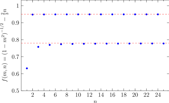
Figure 2: The function (4.26) for the numerical mass spectrum in the MN background.

From the massless scalar equation (4.10), which describes both the third component of $\mathfrak{a}$ and the spin-2 field $\mathfrak{e}^{i}_{j}$, we have not found any discrete mass states, confirming the analytical result of Sec. 4.2.

5 Klebanov-Strassler system

5.1 KS Background

The effective 5-d model describing the bulk dynamics of the KS system contains seven scalar fields. We will use the Papadopoulos-Tseytlin [38] variables $(x,p,y,\Phi,b,h_{1},h_{2})$. In the following, we shall briefly summarize the general relations for this system and the KS background solution. For more details, see our earlier paper [11] and references therein.

The sigma-model metric is

$$G_{ab}\partial_{\mu}\phi^{a}\partial^{\mu}\phi^{b}=\partial_{\mu}x\partial^{\mu}x+6\partial_{\mu}p\partial^{\mu}p+\frac{1}{2}\partial_{\mu}y\partial^{\mu}y+\frac{1}{4}\partial_{\mu}\Phi\partial^{\mu}\Phi+\frac{P^{2}}{2}\operatorname{e}^{\Phi-2x}\partial_{\mu}b\partial^{\mu}b+\\ +\frac{1}{4}\operatorname{e}^{-\Phi-2x}\left[\operatorname{e}^{-2y}\partial_{\mu}(h_{1}-h_{2})\partial^{\mu}(h_{1}-h_{2})+\operatorname{e}^{2y}\partial_{\mu}(h_{1}+h_{2})\partial^{\mu}(h_{1}+h_{2})\right]~{},$$ (5.1)

and the superpotential reads

$$W=-\frac{1}{2}\left(\operatorname{e}^{-2p-2x}+\operatorname{e}^{4p}\cosh y\right)+\frac{1}{4}\operatorname{e}^{4p-2x}\left(Q+2Pbh_{2}+2Ph_{1}\right)~{}.$$ (5.2)

Here, $Q$ and $P$ are constants related to the number of D3-branes and wrapped D5-branes, respectively.

It is useful to introduce the KS radial variable $\tau$ by

$$\partial_{\tau}=\operatorname{e}^{-4p}\partial_{r}~{}.$$ (5.3)

Here and henceforth, a field variable denotes the background of that field ($p$ in this case), while the sigma-model covariant $\mathfrak{a}$ will be used for fluctuations. In terms of $\tau$, the KS background solution of (2.4) is given by

$$\Phi =\Phi_{0}~{},$$ (5.4)

$$\operatorname{e}^{y} =\tanh(\tau/2)~{},$$ (5.5)

$$b =-\frac{\tau}{\sinh\tau}~{},$$ (5.6)

$$h_{1} =-\frac{Q}{2P}+P\operatorname{e}^{\Phi_{0}}\coth\tau(\tau\coth\tau-1)~{},$$ (5.7)

$$h_{2} =P\operatorname{e}^{\Phi_{0}}\frac{\tau\coth\tau-1}{\sinh\tau}~{},$$ (5.8)

$$\frac{2}{3}\operatorname{e}^{6p+2x} =\coth\tau-\frac{\tau}{\sinh^{2}\tau}~{},$$ (5.9)

$$\operatorname{e}^{2x/3-4p} =2P^{2}\operatorname{e}^{\Phi_{0}}3^{-2/3}h(\tau)\sinh^{4/3}\tau~{},$$ (5.10)

with

$$h(\tau)=\int\limits_{\tau}^{\infty}\,\mathrm{d}\vartheta\,\frac{\vartheta\coth\vartheta-1}{\sinh^{2}\vartheta}\left[2\sinh(2\vartheta)-4\vartheta\right]^{1/3}~{}.$$ (5.11)

Moreover, one can show that the warp function $A$ satisfies

$$\operatorname{e}^{-2A-8p}\sim\left(\operatorname{e}^{-6p-2x}\sinh\tau\right)^{2/3}h(\tau)~{},$$ (5.12)

where the proportionality factor depends on an integration constant that sets the 4-d momentum scale.

5.2 KS spin-2 spectrum

Table 2: Mass spectrum of spin-2 glueballs in the KS background ($m^{2}<100$), and comparison with Krasnitz’ WKB results [40]. Krasnitz’ values have been normalized such that the seventh masses (the highest he calculated) agree.

$n$	Krasnitz
1	1.06
2	2.39
3	4.52
4	6.65
5	9.62
6	13.1
7	17.1

$n$	$m^{2}$	$n$	$m^{2}$	$n$	$m^{2}$
1	1.044	8	21.62	15	68.78
2	2.369	9	26.73	16	77.69
3	4.227	10	32.38	17	87.15
4	6.624	11	38.57	18	97.15
5	9.561	12	45.31
6	13.04	13	52.59
7	17.06	14	60.41

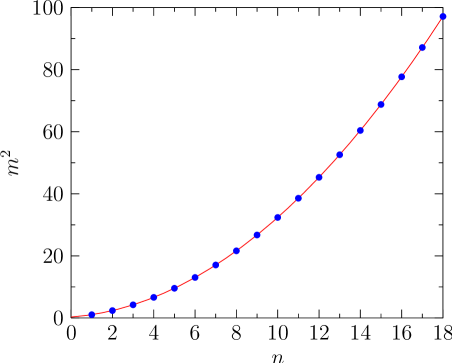
Figure 3: Mass-squared values of spin-2 states. The solid line represents the fit (5.19).

Let us start the numerical analysis of fluctuations in the KS background with the simplest case: the free massless scalar describing the transverse traceless components of fluctuations of the bulk metric. Specifically, we are interested in the spectrum of spin-2 glueballs, expanding on earlier work by Krasnitz [7, 40].

The equation of motion (2.6), after substituting the appropriate relations from the previous subsection, takes the form

$$\left(\partial_{\tau}^{2}+2\operatorname{e}^{-6p-2x}\partial_{\tau}-k^{2}\operatorname{e}^{-2A-8p}\right)\mathfrak{e}=0~{},$$ (5.13)

where we omitted tensor indices on $\mathfrak{e}$. Defining

$$I(\tau)=\frac{h(\tau)}{h(0)}$$ (5.14)

and appropriately choosing the integration constant in the warp function (5.12) such that

$$\operatorname{e}^{-2A-8p}=\left(\operatorname{e}^{-6p-2x}\sinh\tau\right)^{2/3}I(\tau)~{},$$ (5.15)

we can rewrite (5.13) as

$$\left\{\partial_{\tau}^{2}+2\operatorname{e}^{-6p-2x}\partial_{\tau}-k^{2}I(\tau)\left(\operatorname{e}^{-6p-2x}\sinh\tau\right)^{2/3}\right\}\mathfrak{e}=0~{}.$$ (5.16)

The choice of momentum scale normalization in (5.15) is a little unusual, but convenient in what follows.

In this simple one-component system, the method described in Sec. 3.1 is sufficiently robust. For this method, first we need to find the regular behaviour at $\tau=0$, from which the initial conditions will be inferred. For small $\tau$, we find to leading order $\operatorname{e}^{-6p-2x}\approx 1/\tau$ and $I(\tau)\approx 1$, so that a regular solution of (5.16) is found to behave as

$$\mathfrak{e}_{\text{reg}}=1+\frac{k^{2}}{6}\tau^{2}+\mathcal{O}\left(\tau^{4}\right)~{},$$ (5.17)

whereas the singular behaviour, which starts with $1/\tau$, is discarded. Notice that the choice of momentum scale in (5.15) makes the $k^{2}$ term in (5.17) independent of $h(0)$, a good thing since the value of $h(0)$ is known only from numerical evaluation of (5.11).

The second step of this method is to consider the asymptotic UV region. For large $\tau$ we have, again to leading order, $\operatorname{e}^{-6p-2x}\approx 2/3$ and $I(\tau)\sim\tau\operatorname{e}^{-4\tau/3}$. Therefore, the generic dominant asymptotic behaviour is just

$$\mathfrak{e}_{\text{dom}}=1+\mathcal{O}\left(\operatorname{e}^{-2\tau/3}\right)~{}.$$ (5.18)

This tells us that we must simply search for values of $k^{2}$ for which the regular solution tends to zero for large $\tau$.

We find a discrete spectrum of spin-2 states, the first of which are reported and compared to Krasnitz’ values in Table 2. Krasnitz’ results, which were obtained using a WKB approximation, are in good agreement with ours. As shown in Fig. 3, the spectrum fits nicely to a quadratic curve. A least-square fit yields

$$m^{2}\approx 0.2715\,n^{2}+0.4936\,n+0.2969~{}.$$ (5.19)

As we will find in the next section, the coefficient of the $n^{2}$ term enjoys a certain degree of universality.

5.3 KS 7-scalar system: Setup

Now, we turn to the most difficult system of our paper: the seven coupled scalar fields in the KS background. All scalars appear to be fully coupled in the bulk, but we follow the insight gleaned from the “moderate UV” approximation [11] to decouple a $4\times 4$ set of fields (the “glueball sector”) from a $3\times 3$ set (the “gluinoball sector”) to leading order in the UV, as will be seen in Sec. 5.4. The system of field equations we consider follows from (2.5) upon changing the radial coordinate to $\tau$. One finds

$$\left[(\partial_{\tau}-M)(\partial_{\tau}-N)-k^{2}\operatorname{e}^{-2A-8p}\right]\mathfrak{a}=0~{},$$ (5.20)

where we have dropped the tensor indices, and the matrices $M$ and $N$ are defined by

$$\begin{split}M^{a}_{~{}b}&=-N^{a}_{~{}b}-K^{a}_{~{}b}-2\operatorname{e}^{-2x-6p}\delta^{a}_{b}~{},\\ N^{a}_{~{}b}&=\operatorname{e}^{-4p}\left(\partial_{b}W^{a}-\frac{W^{a}W_{b}}{W}\right)~{},\\ K^{a}_{~{}b}&=2\operatorname{e}^{-4p}\mathcal{G}^{a}_{\;\;bc}W^{c}~{}.\end{split}$$ (5.21)

As before, we fix the momentum scale as in (5.15).

Now, the matrices $M$ and $N$ a priori depend on the constants $P$ and $\Phi_{0}$. However, there is a linear field transformation that removes this dependence from (5.20). This implies that these constants can affect the mass spectrum only by an overall change of the momentum scale, which is not visible in our effective 5-d approach. Starting with the fluctuation vector $\mathfrak{a}=(\delta x,\delta p,\delta y,\delta\Phi,\delta b,\delta h_{1},\delta h_{2})^{T}$, the linear transformation that accomplishes this is $\mathfrak{a}^{\prime}=R\mathfrak{a}$ with

$$\mathfrak{a}^{\prime}=\left(\delta x,\delta p,\frac{\delta h_{1}}{P\operatorname{e}^{\Phi_{0}}},\delta\Phi,\delta y,\delta b,\frac{\delta h_{2}}{Pe^{\Phi_{0}}}\right)^{T}$$ (5.22)

and we also rotate the matrices by, e.g., $N^{\prime}=RNR^{-1}$. Henceforth, we shall consider the rotated matrices, dropping primes. The somewhat lengthy expressions for the rotated matrices $K$ and $N$ (that are now independent of $P$ and $\Phi_{0}$ as advertised) as well as the sigma-model metric $G$ can be found in Appendix C.1.

5.4 KS 7-scalar system: Boundary conditions

In this section, we will consider the asymptotic (large-$\tau$) and deep-IR (small-$\tau$) behaviour of the solutions of (5.20), which are needed to fix the boundary (initial) conditions for the numerical integration.

Let us start with the large-$\tau$ region. Asymptotically, the matrices and the warp term in (5.20) can be expanded in powers of $\operatorname{e}^{-\tau}$, such that

$$K=K^{(0)}+\operatorname{e}^{-\tau}K^{(1)}+\mathcal{O}\left(\operatorname{e}^{-2\tau}\right)~{},\quad N=N^{(0)}+\operatorname{e}^{-\tau}N^{(1)}+\mathcal{O}\left(\operatorname{e}^{-2\tau}\right)~{}.$$ (5.23)

In what follows, we can always drop the $\mathcal{O}\left(\operatorname{e}^{-2\tau}\right)$ terms (the reason for this will become clearer later on, cf. the discussion below (5.40)). For the sake of brevity, we write the matrices in block form,

$$K=\begin{pmatrix}K_{4\times 4}&K_{4\times 3}\\ K_{3\times 4}&K_{3\times 3}\end{pmatrix}~{},$$ (5.24)

and analogously for $N$. Then, the matrices in (5.23) are

$$K^{(0)}_{4\times 4} =\begin{pmatrix}0&0&\frac{2}{3(\tau-1/4)}&0\\ 0&0&0&0\\ -2&0&-\frac{1}{\tau-1/4}&-1\\ 0&0&\frac{4}{3(\tau-1/4)}&0\end{pmatrix}~{},$$ (5.25)

$$K^{(0)}_{3\times 3} =\begin{pmatrix}0&0&-\frac{4}{3(\tau-1/4)}\\ 0&-\frac{1}{\tau-1/4}&0\\ 2&0&-\frac{1}{\tau-1/4}\end{pmatrix}~{},$$ (5.26)

$$K^{(0)}_{4\times 3} =K^{(0)}_{3\times 4}=0~{},$$ (5.27)

$$N^{(0)}_{4\times 4} =\begin{pmatrix}-\frac{1}{\tau+1/4}&-\frac{4\tau-1}{\tau+1/4}&-\frac{2}{3(\tau+1/4)}&0\\ -\frac{2(\tau-1/4)}{3(\tau+1/4)}&-\frac{2(\tau+5/4)}{3(\tau+1/4)}&\frac{2}{9(\tau+1/4)}&0\\ \frac{1}{\tau+1/4}&\frac{4\tau-1}{\tau+1/4}&\frac{2}{3(\tau+1/4)}&1\\ 0&0&0&0\end{pmatrix}~{},$$ (5.28)

$$N^{(0)}_{3\times 3} =\begin{pmatrix}-1&0&0\\ 0&0&1\\ -2&1&0\end{pmatrix}~{},$$ (5.29)

$$N^{(0)}_{4\times 3} =N^{(0)}_{3\times 4}=0~{},$$ (5.30)

and

$$K^{(1)}_{4\times 3} =\begin{pmatrix}0&\frac{4(\tau-1)}{3(\tau-1/4)}&-\frac{4\tau}{3(\tau-1/4)}\\ 0&0&0\\ -4(\tau-2)&0&4\\ 0&-\frac{8(\tau-1)}{3(\tau-1/4)}&-\frac{8\tau}{3(\tau-1/4)}\end{pmatrix}~{},$$ (5.31)

$$K^{(1)}_{3\times 4} =\begin{pmatrix}0&0&\frac{8\tau}{3(\tau-1/4)}&0\\ -4(\tau-1)&0&0&2(\tau-1)\\ 4(\tau-2)&0&4&2(\tau-2)\end{pmatrix}~{},$$ (5.32)

$$K^{(1)}_{4\times 4} =K^{(1)}_{3\times 3}=0~{},$$ (5.33)

$$N^{(1)}_{4\times 3} =\begin{pmatrix}\frac{1}{\tau+1/4}&-\frac{4(\tau-1)}{3(\tau+1/4)}&\frac{4\tau}{3(\tau+1/4)}\\ \frac{2(\tau-1/4)}{3(\tau+1/4)}&\frac{4(\tau-1)}{9(\tau+1/4)}&-\frac{4\tau}{9(\tau+1/4)}\\ \frac{4\tau^{2}-5\tau-5/2}{\tau+1/4}&\frac{16\tau-1}{3(\tau+1/4)}&-\frac{4\tau}{3(\tau+1/4)}\\ 0&0&0\end{pmatrix}~{},$$ (5.34)

$$N^{(1)}_{3\times 4} =\begin{pmatrix}\frac{2}{\tau+1/4}&\frac{8(\tau-1/4)}{\tau+1/4}&\frac{4}{3(\tau+1/4)}&0\\ \frac{2(\tau-1)}{\tau+1/4}&\frac{8(\tau-1)(\tau-1/4)}{\tau+1/4}&\frac{4(\tau-1)}{3(\tau+1/4)}&-2(\tau-1)\\ -\frac{2(\tau-2)}{\tau+1/4}&-\frac{8(\tau-2)(\tau-1/4)}{\tau+1/4}&-\frac{4(\tau-2)}{3(\tau+1/4)}&-2(\tau-2)\end{pmatrix}~{},$$ (5.35)

$$N^{(1)}_{4\times 4} =N^{(1)}_{3\times 3}=0~{}.$$ (5.36)

The transformation $\mathfrak{a}\rightarrow\mathfrak{a}^{\prime}$, cf. (5.22), has brought the matrices into this nice block form. We also need

$$\operatorname{e}^{-2x-6p}=\frac{2}{3}+\mathcal{O}\left(\operatorname{e}^{-2\tau}\right)$$ (5.37)

as well as

$$\operatorname{e}^{-2A-8p}=\frac{3^{1/3}}{h(0)}\left(\tau-\frac{1}{4}\right)\operatorname{e}^{-2\tau/3}\left[1+\mathcal{O}\left(\operatorname{e}^{-2\tau}\right)\right]~{}.$$ (5.38)

It is a useful check that the leading-order terms of these expressions coincide with the respective quantities evaluated in the Klebanov-Tseytlin background [24].

Since (5.38) is exponentially suppressed, the leading order terms of the asymptotic solutions will be independent of the momentum $k$. We note that this is just as we assumed in Sec. 2.3. In contrast, in the MN system, the asymptotic behaviours of the solutions depend on $k$ [cf. (4.13)].

The asymptotic UV solutions, including the leading and some subleading terms, are found by iteratively solving the equations

$$\left(\partial_{\tau}-N^{(0)}\right)\phi^{(n)} =\psi^{(n)}+\operatorname{e}^{-\tau}N^{(1)}\phi^{(n-1)}~{},$$ (5.39)

$$\left(\partial_{\tau}-M^{(0)}\right)\psi^{(n)} =\beta\left(\tau-\frac{1}{4}\right)\operatorname{e}^{-2\tau/3}\phi^{(n-1)}+\operatorname{e}^{-\tau}M^{(1)}\psi^{(n-1)}~{},$$ (5.40)

where $\beta=3^{1/3}k^{2}/h(0)$, and we set $\phi^{(-1)}=\psi^{(-1)}=0$. The solutions $\phi^{(0)}$ are the leading order terms of the asymptotic solutions. Again, we will drop all $\mathcal{O}\left(\operatorname{e}^{-2\tau}\right)$ terms in the iteration. The reason for this is the following. Dropping subleading terms in the initial conditions leads to systematic errors in the numerical solutions, which must obviously be kept smaller than the relevant parts of the solutions. This implies that the initial conditions of all behaviours we use must be given to the same order in $\operatorname{e}^{-\tau}$. We will use the mid-point method of Sec. 3.2, in which only the subdominant asymptotic behaviours are needed. Now, the leading term of the weakest subdominant behaviour goes like $\operatorname{e}^{-8\tau/3}$, whereas the strongest subdominant behaviour goes like $\operatorname{e}^{-\tau}$. Thus, they differ by $\operatorname{e}^{-5\tau/3}$ and we can drop $\mathcal{O}\left(\operatorname{e}^{-2\tau}\right)$ corrections.

The somewhat lengthy expressions of the asymptotic solutions are deferred to Appendix C.2.

Now, let us consider the small-$\tau$ region. In order to find the independent behaviours for small $\tau$, we expand the matrices in (5.20) about $\tau=0$ and make an ansatz of the form

$$\mathfrak{a}(\tau)=\tau^{q}\left(\mathfrak{a}_{0}+\tau\mathfrak{a}_{1}+\tau^{2}\mathfrak{a}_{2}+\tau^{3}\mathfrak{a}_{3}+\cdots\right)~{},$$ (5.41)

with some undetermined number $q$, and constant vectors $\mathfrak{a}_{n}$, $n=0,1,2,\ldots$. These are then determined recursively from the equation of motion (using computer algebra). It turns out that, of the 14 solutions, there exist four solutions with $q=0$, one with $q=1$, three with $q=2$, four with $q=-1$, and one each with $q=-2$ and $q=-3$. Thus, there exist eight solutions, whose components are finite at $\tau=0$, and six with singular component behaviour. However, the regularity condition (2.10) tells us that one of the solutions with $q=0$ is, in fact, singular. Therefore, we arrive at precisely seven regular and seven singular solutions. The independent small-$\tau$ behaviours are listed in Appendix C.3.

5.5 KS spin-0 spectrum

Analogously to the MN case, instead of 7 coupled 2nd order ODEs, it is more convenient to solve 14 coupled 1st order ODEs. Thus, let us rewrite (5.20) as

$$\partial_{\tau}\begin{pmatrix}\mathfrak{a}\\ \mathfrak{b}\end{pmatrix}=\begin{pmatrix}N&1\\ k^{2}\operatorname{e}^{-2A-8p}&M\end{pmatrix}\begin{pmatrix}\mathfrak{a}\\ \mathfrak{b}\end{pmatrix}~{}.$$ (5.42)

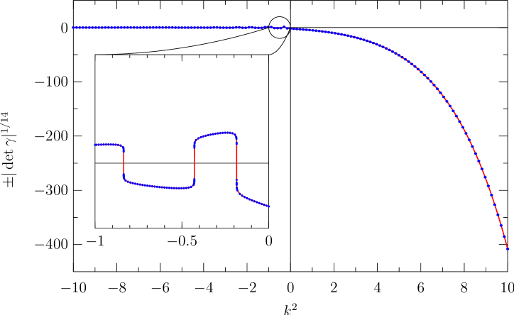
Figure 4: $\det\gamma$ as a function of $k^{2}$. For clarity, we have taken the 14th root of the absolute value of the determinant (leaving its sign untouched). The plot shows clearly that there are no zero crossings for positive $k^{2}$. The inset shows the zeros of $\det\gamma$ for the first three spin-0 states.

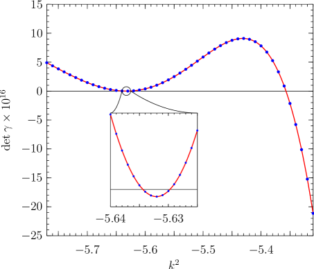
Figure 5: Here we plot $\det\gamma$ in the range $k^{2}\in[-5.8\ldots-5.3]$. The inset zooms in on the region around $k^{2}=-5.63$, where there are two zeros.

$m^{2}$	0.185	0.428	0.835	1.28	1.63	1.94	2.34
	2.61	3.32	3.54	4.12	4.18	4.43	4.43
	5.35	5.63	5.63	6.59	6.66	6.77	7.14

Table 3: Low-lying Klebanov-Strassler spin-0 mass states, extracted from zero-crossings in Fig. 4. More values are given in Appendix D.

We apply the midpoint determinant method as outlined in section 3.2. That is, we compute the $14\times 14$ matrix

$$\gamma=\begin{pmatrix}\mathfrak{a}_{\mathrm{reg}}{}&\mathfrak{a}_{\mathrm{sub}}{}\\ \mathfrak{b}_{\mathrm{reg}}{}&\mathfrak{b}_{\mathrm{sub}}{}\end{pmatrix}_{\tau=\tau_{\rm mid}}$$ (5.43)

as a function of $k^{2}$ and look for zero crossings of $\det\gamma$. A rough plot of $\det\gamma$ is shown in Fig. 4. We verify that there are no zero crossings for positive $k^{2}$. The zero crossings of $\det\gamma$ can be found by zooming in on a particular region of the plot, as shown, for example, in the inset. As the determinant itself changes over many orders of magnitude, it is useful to plot $\pm|\det\gamma|^{1/14}\equiv\mathrm{sign}(\det\gamma)|\det\gamma|^{1/14}$ instead. The sharp turns in the inset are merely artifacts of this, as is apparent from Fig. 5, where $\det\gamma$ itself is displayed without the 14th root, and there are no sharp turns.

We have calculated all mass values up to $m^{2}=600$. The first few are listed in Table 3; for a more extended list see Table 5 in Appendix D. Our results exhibit two interesting features. First, it appears that several mass values are nearly degenerate, such as the two values about $m^{2}\approx 4.43$ and two values about $m^{2}\approx 5.63$. The origin of this in our calculation can be seen in Fig. 5: The $\det\gamma$ curve barely seems to touch the $k^{2}$-axis, and only zooming in reveals that there are two crossings. As we do not have a dynamical explanation of it, it is possible that this near degeneracy is accidental, or it may indicate a multiplet originating from a weakly broken symmetry of the low-energy effective theory.

The second interesting feature is the appearance, for large masses, of a periodic pattern of period 7 in the consecutive spectrum excitation number $n$. On the left hand side of Fig. 6, this pattern is easily visible. Hence, we split the spectrum into 7 towers of mass states, one of which is shown on the right hand side of Fig. 6. From now on, we distinguish excitation numbers of individual towers, denoted by $n_{t}$, from the excitation number $n$ of the whole spin-0 spectrum.

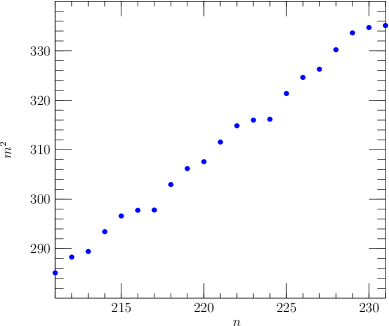
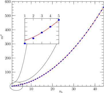
Figure 6: On the left, we see that for high $m^{2}$, it is easy to identify the periodicity “empirically” as 7. On the right, we have extracted one tower (i.e., every 7th point) from the full spectrum, enumerated states in that tower by a parameter $n_{t}$ (the “excitation number”) and fit those points to a quadratic curve starting with the third point. As shown in the inset, $m^{2}\sim n_{t}^{2}$ is not a good description for very low $n_{t}$, unlike in the spin-2 case.

Like the spin-2 spectrum, the seven spin-0 spectra also exhibit quadratic dependence of $m^{2}$ on excitation number $n_{t}$. Leaving out the first two values of each tower (i.e. $n_{t}=1,2$) least square fits of the “large $m^{2}$” behavior (using mass values up to $m^{2}=600$) yield

$$\begin{split}m^{2}&\approx 0.271\,n_{t}^{2}+0.774\,n_{t}+0.562~{},\\ m^{2}&\approx 0.270\,n_{t}^{2}+0.928\,n_{t}-0.430~{},\\ m^{2}&\approx 0.275\,n_{t}^{2}+0.769\,n_{t}+1.921~{},\\ m^{2}&\approx 0.272\,n_{t}^{2}+1.017\,n_{t}+1.023~{},\\ m^{2}&\approx 0.272\,n_{t}^{2}+1.119\,n_{t}+0.337~{},\\ m^{2}&\approx 0.271\,n_{t}^{2}+1.150\,n_{t}+0.648~{},\\ m^{2}&\approx 0.273\,n_{t}^{2}+1.082\,n_{t}+2.544~{}.\end{split}$$ (5.44)

The last digit of the leading coefficients (i.e. the coefficients of the $n_{t}^{2}$ terms) can vary slightly if one performs the fits with more than two states from each tower left out. Still, it is obvious that within some uncertainties the leading coefficients all coincide rather well, both amongst each other and also with the coefficient of the spin-2 tower (5.19), leading to roughly universal behaviour at large $n_{t}$.

5.6 KS 7-scalar system: Quadratic confinement

If one plots the experimental values for squared meson masses $m^{2}$ (e.g. for the first few resonances of the $\rho$ meson) against their consecutive number $n$, the data obeys $m^{2}\sim n$ to good accuracy. One might call this “linear confinement”. Karch, Katz, Son and Stephanov (KKSS) [17] emphasized that there are no known supergravity backgrounds that reproduce this experimental fact about mesons from AdS/CFT.

In fact, the claim of KKSS was even stronger (p. 13): that for all known supergravity backgrounds $m^{2}\sim n^{2}$, which is “quadratic confinement”. Extending these arguments to our setting, one might expect to see quadratic confinement in, say, the Klebanov-Strassler background. A priori, given the complexity of fluctuations around the Klebanov-Strassler solution, one could have expected that no such general statement could be made except possibly in some extreme asymptotic regime.

This expectation turns out to be wrong. Although we cannot be absolutely sure from our analysis, the KKSS claim that $m^{2}\sim n^{2}$ seems resoundingly apparent in Fig. 6 and the fits (5.44). Since the KS theory is in any case not QCD, linear confinement is not crucial to have, but our results strengthen the case for finding controllable models that do exhibit linear confinement (the metric-scalar model given in [17] seems promising, but so far has not been shown to be the solution of any known theory).

Of course, one would expect that much of the low-energy dynamics of the theory would be determined by the lowest-lying mass states, and they have a richer structure than the large-$n$ asymptotics — a glimpse of this can be seen in the inset on the right hand side of Fig. 6. Since the KS theory incorporates spontaneous breaking of chiral symmetry, this should have left its mark on our spectrum. We do observe some interesting patterns, but we have not been able to link them conclusively to symmetry breaking. This deserves further study.

As alluded to in the introduction, operator mixing is even more subtle here than in standard AdS/CFT. We have computed the spin-0 mass spectrum, but we have not said what the mass states are composed of in terms of dual gauge theory operators. Some of the problems of identifying the mass states were already addressed in section 2.3, i.e. the ambiguity in the normalization of the dominant asymtptotic solutions and the freedom to add to a given dominant solution multiples of asymptotic solutions of equal or weaker strength. Thus we do not attempt to give a further interpretation of the mass states. We just content ourselves by noticing that there is actually a quantity that is easy to obtain with our method, namely the coefficients $d_{\lambda,i}$ from (2.28). These can be determined straightforwardly by solving (3.8) at the various mass values. This gives information on the composition of the “cavity mode” (that we called $\mathfrak{a}_{\lambda}$ in chapter 2) corresponding to a mass state in terms of our basis of subdominant solutions. However, as the interpretation in terms of operator mixing is not clear to us, we refrain from determining these coefficients explicitly here. Moreover, also the quantities $Z_{\lambda,i}$, defined in (2.33), could be determined in principle. They correspond to the residues of the mass poles if $N_{\lambda}$, introduced in (2.32), is really one, as in the case of asymptotic AdS spaces (see Appendix A).

5.7 Comparison to hardwall approximations

values from Table 3	$\tau_{\rm IR}=0.5$	$\tau_{\rm IR}=0.75$	$\tau_{\rm IR}=1$
0.19	0.27	0.30	0.34
0.42	0.56	0.63	0.71
0.83	0.86	1.03	1.14
1.29	1.39	1.62	1.83
1.63	1.78	1.89	2.03
1.94	2.32	2.42	2.57
2.35	2.43	2.56	2.75
2.61	3.26	3.39	3.70
3.33	3.58	3.80	4.09
3.53	4.06	4.22	4.40
4.13	4.30	4.60
4.17	4.54	4.81
4.43 (2x)	4.71

Table 4: Comparison of our mass values with a toy hardwall model as described in the text (only values up to $m^{2}=5$ are included). This demonstrates that the spectrum indeed strongly depends on the IR dynamics.

In this section, we would like to give some arguments supporting our conviction stated in the introduction that the detailed form of the spectrum depends crucially on the details of the IR dynamics in the gauge theory. Holographically, this means that it is important to use the full Klebanov-Strassler background to determine the low lying mass eigenvalues. To illustrate this, we compare our spectrum with a naive toy hardwall model. In particular, one might hope to find the right spectrum by using the Klebanov-Tseytlin approximation of the KS background. This is roughly equivalent to cutting off the KS background at some value $\tau_{\rm IR}$ of order one (the two solutions differ strongly only for $\tau\leq 0.8$). In order to use the determinant method described in Sec. 3.1, one would like to impose seven independent initial conditions at $\tau_{\rm IR}$ and then solve the equations numerically from the IR towards the UV. One again demands that there is a linear combination of those numerical solutions that does not contain any dominant solutions $\mathfrak{a}_{\rm dom}$ when expanded in a basis of asymptotic solutions. Lacking any guiding principle for choosing these initial conditions, we arbitrarily impose that all components of the seven scalar fields should vanish at $\tau_{\rm IR}$, whereas for each initial condition one of the first derivatives are taken to be unity. This gives seven independent initial conditions. The resulting spectrum is contained in Table 4 for several values of $\tau_{\rm IR}$, together with the correct mass values. Obviously, the “toy spectra” depend on the value of $\tau_{\rm IR}$, but they also differ strongly from the correct values. We believe that this holds more generally, even if one had a different set of initial conditions than these, whether or not they are physically motivated.

To summarize, we do not see any way of implementing a hard-wall approximation that reproduces the correct spectrum of Table 3.

6 Outlook

We have computed spin-0 and spin-2 mass spectra for the Maldacena-Nunez (wrapped D5-brane) and Klebanov-Strassler (warped deformed conifold) backgrounds. Although fairly complicated, there are some simple features. For example, for large excitation number $n$, the spin-0 states in the KS theory organize into 7 towers, each of which displays quadratic confinement, in agreement with the claims of [17]. (“Large” is not terribly large; around $n\geq 3$.) For low excitation number $n$, there is a rich structure of mass values, which exhibits interesting patterns of near degeneracy.

For the Maldacena-Nunez background, our numerical results confirm the rough features of the analytic spectra we derived in [11] and improved upon here; the discrete mass spectrum has an upper bound, which is quite different from the KS case.

The situation with respect to other studies of glueball spectra in these backgrounds, based on various truncations, has not changed from [11]. The one result we have been able to compare our results to is the set of mass states for spin-2 glueballs in KS, where the first few values were computed in the WKB approximation by Krasnitz in [40], and are roughly correct, as in Table 2.

It would be very important to understand the details of mixing in this context; without further information along the lines we have suggested, we cannot determine the composition of the mass states we find. On the good side, the spectrum we have found is unique, in that the variables used to find it are gauge-invariant, and we impose the boundary conditions one really wants to impose, rather than approximations thereof.

These results and methods could straightforwardly be applied to other gauge/gravity dual pairs. Apart from other $\mathcal{N}=1$ dualities, it would be interesting to apply these methods also in $\mathcal{N}=0$ gauge theory. There, the existence of a simple superpotential $W$, which greatly simplified our task, is not guaranteed but occurs e.g. for $\mathcal{N}=0$ backgrounds with “pseudo-Killing” spinors (cf. for example [21]). Here is a concrete question: do the meson spectra computed in other backgrounds contain glueball admixtures from the $e^{-\phi}$ in the DBI action?

Independently of supersymmetry breaking, including probe branes in Klebanov-Strassler à la [18, 19] would be interesting to study using our methods.

Finally, the greatest challenge for holography in presently known confining backgrounds is to compute correlators from the Klebanov-Strassler background. Some progress was made in [7, 41, 40, 42, 43]. We considered the Krasnitz (extreme high-energy) limit in [11] and found some analytical solutions. However, those solutions were checked to be valid around $k^{2}\sim 10^{6}$, whereas in this paper, we were interested in IR physics, and thus the Krasnitz approximation was not available to us. In fact, we only considered solutions up to $k^{2}\sim 2000$, and going much higher presents a numerical difficulty, as one needs to go increasingly far in the UV for the solutions to become asymptotic, so that the determinant method is applicable. This is a superable challenge for connecting the high-energy and low-energy regimes, which might ultimately be the most useful aspect of holography for confining gauge theories. We hope to return to these issues in future publications.

Appendix A Some 2-point functions in AdS/CFT

In this section, we review how the 2-point functions for some known cases of AdS/CFT arise as sums over the spectrum of bulk eigenfunctions, using expressions developed in the main text.

A.1 AdS bulk

Let us start with a set of $n$ free massive scalar fields on $(d+1)$-dimensional AdS bulk space. Using the language of Sec. 2, we will derive the 2-point function as a “sum” over the spectrum of bulk eigenfunctions. (For pure AdS the spectrum is continuous, so the “sum” is in fact an integral. This will be different in the next subsection.) When the smoke has cleared (in (A.14)), the connection to the standard computation in terms of the IR-regular Bessel function $\operatorname{K}_{\nu}(kz)$ will be evident.

The bulk equation of motion (2.5) (in $d$-momentum space) is

$$\left(\partial_{z}^{2}-\frac{d-1}{z}\partial_{z}-\frac{m^{2}}{z^{2}}-k^{2}\right)\phi=0~{},$$ (A.1)

where $z=\operatorname{e}^{-r}$ is the radial coordinate. We have omitted the field indices, and $m^{2}$ is to be understood as a diagonal matrix with entries $m_{i}^{2}$, $i=1,\ldots,n$. The conformal dimensions of the operators $\mathcal{O}_{i}$ dual to the components of $\phi$ are related to the mass parameters $m_{i}$ by

$$\Delta_{i}=\frac{d}{2}+\alpha_{i}~{},\qquad\alpha_{i}=\sqrt{\frac{d^{2}}{4}+m_{i}^{2}}~{}.$$ (A.2)

Small values of $z$ give the asymptotic UV region, whereas large $z$ describe the bulk interior (IR region).

Conventionally normalized asymptotic solutions of (A.1) are

$$\phi_{\mathrm{dom}}{}_{i}^{a}(z,k) =\delta^{a}_{i}\Gamma(1-\alpha_{i})\left(\frac{k}{2}\right)^{\alpha_{i}}z^{d/2}\operatorname{I}_{-\alpha_{i}}(kz)=\delta^{a}_{i}\,z^{d/2-\alpha_{i}}+\cdots~{},$$ (A.3)

$$\phi_{\mathrm{sub}}{}_{i}^{a}(z,k) =\delta^{a}_{i}\Gamma(1+\alpha_{i})\left(\frac{k}{2}\right)^{-\alpha_{i}}z^{d/2}\operatorname{I}_{\alpha_{i}}(kz)=\delta^{a}_{i}\,z^{d/2+\alpha_{i}}+\cdots~{},$$ (A.4)

where the $\operatorname{I}_{\alpha}$ are modified Bessel functions, and after the second equal signs we indicated just the respective leading behaviours. The powers of $k$ in front of the solutions are necessary in order to make the leading terms $k$-independent, while the remaining coefficients are conventional normalizations.

For asymptotically AdS bulk backgrounds, (A.1) still holds in the asymptotic region. Therefore, the leading behaviours of the asymptotic solutions remain as in (A.3) and (A.4),

$$\phi_{\mathrm{dom}}{}_{i}^{a}(z,k)=\delta^{a}_{i}\,z^{d/2-\alpha_{i}}+\cdots~{},\qquad\phi_{\mathrm{sub}}{}_{i}^{a}(z,k)=\delta^{a}_{i}\,z^{d/2+\alpha_{i}}+\cdots~{}.$$ (A.5)

The general form of the matrix $Z_{ij}$ (2.30) in asymptotically AdS spaces follows easily. One finds

$$Z_{ij}=2\alpha_{i}\,\delta_{ij}~{}.$$ (A.6)

A general result of holographic renormalization [34, 35, 36] is that (the non-local part of) the exact one-point function $\left\langle{\mathcal{O}_{i}}\right\rangle_{\text{exact}}$ is

$$\left\langle{\mathcal{O}_{i}}\right\rangle_{\text{exact}}=2\alpha_{i}\,d_{i}~{}\stackrel{{\scriptstyle\eqref{appads:dim}}}{{=}}\left(2\Delta_{i}-d\right)d_{i}\;.$$ (A.7)

Comparing this with (2.24), one finds

$$Y_{ij}=2\alpha_{i}\,\delta_{ij}=Z_{ij}~{},$$ (A.8)

which, together with (2.32), implies $N_{\lambda}=1$.

Returning to the pure AdS bulk, (A.1) admits a continuous spectrum of regular and subdominant solutions for $k^{2}=-\lambda^{2}$, $\lambda>0$. The eigenfunctions are given by

$$\phi_{\lambda i}^{a}(z)=\delta^{a}_{i}\,\sqrt{\lambda}\,z^{d/2}\operatorname{J}_{\alpha_{i}}(\lambda z)$$ (A.9)

and satisfy the orthogonality relation

$$\int\limits_{0}^{\infty}\frac{\,\mathrm{d}z}{z}z^{-(d-2)}\phi_{\lambda i}(z)\cdot\phi_{\lambda^{\prime}j}(z)=\delta(\lambda-\lambda^{\prime})\delta_{ij}~{}.$$ (A.10)

Considering the small-$z$ behaviour of (A.9), one can read off the response coefficients $d_{\lambda i,j}$,

$$d_{\lambda i,j}=\delta_{ij}\left(\frac{\lambda}{2}\right)^{\alpha_{i}}\frac{\sqrt{\lambda}}{\Gamma(1+\alpha_{i})}~{}.$$ (A.11)

Hence, after using (2.33) and $N_{\lambda}=1$, one obtains for (2.34)

$$\left\langle{\mathcal{O}_{i}(k)\mathcal{O}_{j}(-k)}\right\rangle=\delta_{ij}\frac{2^{2(1-\alpha_{i})}}{\Gamma(\alpha_{i})^{2}}\int\limits_{0}^{\infty}\,\mathrm{d}\lambda\,\frac{\lambda^{2\alpha_{i}+1}}{k^{2}+\lambda^{2}}=-\delta_{ij}\,2\frac{\Gamma(1-\alpha_{i})}{\Gamma(\alpha_{i})}\left(\frac{k}{2}\right)^{2\alpha_{i}}~{}.$$ (A.12)

Notice that the second equality holds only after analytic continuation, because the integral does not exist if $\alpha_{i}\geq 0$. This is equivalent to adding an infinite contact term to the integral over the spectrum. For example, if $0<\alpha_{i}<1$, we rewrite the integrand as

$$\frac{\lambda^{2\alpha_{i}+1}}{k^{2}+\lambda^{2}}=\lambda^{2\alpha_{i}-1}-k^{2}\frac{\lambda^{2\alpha_{i}-1}}{k^{2}+\lambda^{2}}$$ (A.13)

and add a counter term that cancels the first term on the right hand side.

The finite result (A.12) can also be obtained in the usual way, i.e., by considering a regular solution of (A.1),

$$\phi_{i}^{a}(z,k)=\delta_{i}^{a}\frac{2\tilde{d}}{\Gamma(\alpha_{i})}\left(\frac{k}{2}\right)^{\alpha_{i}}z^{d/2}\operatorname{K}_{\alpha_{i}}(kz)~{}=\delta_{i}^{a}\tilde{d}\,\frac{2^{1-\alpha_{i}}}{\Gamma(\alpha_{i})}\int\limits_{0}^{\infty}\,\mathrm{d}\lambda\,\frac{\lambda^{\alpha_{i}+1}}{k^{2}+\lambda^{2}}z^{d/2}\operatorname{J}_{\alpha_{i}}(\lambda z)\;,$$ (A.14)

reading off the relation between the response and source coefficients, $d$ and $\tilde{d}$, with the help of

$$\operatorname{K}_{\alpha}(x)=2^{\alpha-1}\Gamma(\alpha)x^{-\alpha}(1+\ldots)-2^{-\alpha-1}\frac{\Gamma(1-\alpha)}{\alpha}x^{\alpha}(1+\ldots)$$ (A.15)

and then using (A.7). It is interesting to note that the small-$z$ behaviour of the integrand in (A.14) is only subdominant, while the expression in terms of $\operatorname{K}_{\alpha_{i}}$ contains also a dominant piece. The explanation of this apparent discrepancy is the UV part of the spectrum (large $\lambda$), i.e., one cannot find some sufficiently small $z$ such that $\lambda z$ is also small for all values of $\lambda$. Hence, loosely, the UV-part of the spectrum generates the dominant behaviour.

A.2 Active scalar in GPPZ flow

As a second example, let us take the active scalar in the GPPZ flow [44]. Its gauge invariant bulk equation of motion reads [29, 30]

$$\left[u(1-u)\partial_{u}^{2}+(3u-2)\partial_{u}+\frac{3u}{4(1-u)}-1+\frac{k^{2}}{4}\right]\phi=0~{},$$ (A.16)

where the radial coordinate $u$ is defined by $u=1-\operatorname{e}^{-2r}$, and the warp factor is $\operatorname{e}^{2A}=u/(1-u)$.

Eq. (A.16) admits a discrete spectrum of regular and subdominant eigenfunctions, with mass squares

$$m_{n}^{2}=4n(n+1)~{},\qquad n=1,2,3,\ldots\ .$$ (A.17)

The normalized eigenfunctions are

$$\phi_{n}=\sqrt{\frac{2(2n+1)}{n(n+1)}}(1-u)^{3/2}\frac{\,\mathrm{d}}{\,\mathrm{d}u}\operatorname{P}_{n}(2u-1)~{},$$ (A.18)

where $\operatorname{P}_{n}$ are Legendre polynomials. One easily finds the response coefficients

$$d_{n}=\sqrt{2n(n+1)(2n+1)}~{}.$$ (A.19)

Thus, using $\alpha=1$ (we have a $\Delta=3$ operator) and (A.8) (which holds for asymptotically AdS spaces), we obtain for the 2-point function (2.34)

$$\left\langle{\mathcal{O}(k)\mathcal{O}(-k)}\right\rangle=\sum\limits_{n=1}^{\infty}\frac{8n(n+1)(2n+1)}{k^{2}+4n(n+1)}+\text{c.t.}\ .$$ (A.20)

Clearly, the sum in (A.20) does not converge, so that there are again infinite contact terms. It is instructive to compare (A.20) with the finite result from holographic renormalization [45, 46],

$$\left\langle{\mathcal{O}(k)\mathcal{O}(-k)}\right\rangle=\frac{k^{2}}{2}\left[\psi\left(\frac{3+\sqrt{1-k^{2}}}{2}\right)+\psi\left(\frac{3-\sqrt{1-k^{2}}}{2}\right)-\psi(1)-\psi(2)\right]~{},$$ (A.21)

where $\psi(z)=[\ln\Gamma(z)]^{\prime}$. Using the identity

$$\psi(x)-\psi(y)=\sum\limits_{n=0}^{\infty}\left(\frac{1}{y+n}-\frac{1}{x+n}\right)~{},$$ (A.22)

we obtain from (A.21)

$$\begin{split}\left\langle{\mathcal{O}(k)\mathcal{O}(-k)}\right\rangle&=\frac{k^{4}}{2}\sum\limits_{n=1}^{\infty}\frac{2n+1}{n(n+1)[k^{2}+4n(n+1)]}\\ &=\sum\limits_{n=1}^{\infty}\left[\frac{8n(n+1)(2n+1)}{k^{2}+4n(n+1)}-2(2n+1)+k^{2}\frac{2n+1}{2n(n+1)}\right]~{}.\end{split}$$ (A.23)

Again, we see that holographic renormalization makes a precise choice for the contact terms and, therefore, picks a renormalization scheme and scale. Indeed, the finite result (A.21) satisfies the renormalization conditions

$$\left.\left\langle{\mathcal{O}(k)\mathcal{O}(-k)}\right\rangle\right|_{k^{2}=0}=0~{},\qquad\frac{\,\mathrm{d}}{\,\mathrm{d}k^{2}}\left.\left\langle{\mathcal{O}(k)\mathcal{O}(-k)}\right\rangle\right|_{k^{2}=0}=0~{}.$$ (A.24)

Appendix B Matrices for the MN background

The entries of the matrices $M$ and $N$ of Eq. (4.7) for the regular MN background ($c=0$) are

$$\begin{split}M_{11}&=-[(8\rho^{2}-4\rho+1)+\operatorname{e}^{-4\rho}(-64\rho^{3}+112\rho^{2}-48\rho+2)+\\ &\qquad+\operatorname{e}^{-8\rho}(256\rho^{4}-896\rho^{3}+248\rho^{2}+108\rho-17)+\\ &\qquad+\operatorname{e}^{-12\rho}(1536\rho^{4}-736\rho^{2}+28)+\\ &\qquad+\operatorname{e}^{-16\rho}(256\rho^{4}+896\rho^{3}+248\rho^{2}-108\rho-17)+\\ &\qquad+\operatorname{e}^{-20\rho}(64\rho^{3}+112\rho^{2}+48\rho+2)+\operatorname{e}^{-24\rho}(8\rho^{2}+4\rho+1)]/\\ &\quad/\{\rho(1-\operatorname{e}^{-4\rho})^{4}[1-\operatorname{e}^{-4\rho}(4\rho+1)](4\rho-1+\operatorname{e}^{-4\rho})\}\\ M_{12}&=[(3\rho-1)+\operatorname{e}^{-4\rho}(16\rho^{3}-48\rho^{2}+12\rho+2)+\operatorname{e}^{-8\rho}(96\rho^{3}-30\rho)+\\ &\qquad+\operatorname{e}^{-12\rho}(16\rho^{3}+48\rho^{2}+12\rho-2)+\operatorname{e}^{-16\rho}(3\rho+1)]\times\\ &\quad\times 4\operatorname{e}^{-2\rho}/\{\rho(1-\operatorname{e}^{-4\rho})^{3}[1-\operatorname{e}^{-4\rho}(4\rho+1)](4\rho-1+\operatorname{e}^{-4\rho})\}\\ M_{21}&=-[1-\operatorname{e}^{-4\rho}(4\rho+1)](4\rho-1+\operatorname{e}^{-4\rho})[(\rho-1)+\operatorname{e}^{-4\rho}6\rho+\operatorname{e}^{-8\rho}(\rho+1)]\times\\ &\quad\times 4\operatorname{e}^{-2\rho}/[\rho(1-\operatorname{e}^{-4\rho})^{5}]\\ M_{22}&=-[(2\rho-1)+\operatorname{e}^{-4\rho}(32\rho^{3}-128\rho^{2}+56\rho-2)+\\ &\qquad+\operatorname{e}^{-8\rho}(-256\rho^{4}+960\rho^{3}-256\rho^{2}-118\rho+17)+\\ &\qquad+\operatorname{e}^{-12\rho}(-1536\rho^{4}+768\rho^{2}-28)+\\ &\qquad+\operatorname{e}^{-16\rho}(-256\rho^{4}-960\rho^{3}-256\rho^{2}+118\rho+17)+\\ &\qquad+\operatorname{e}^{-20\rho}(-32\rho^{3}-128\rho^{2}-56\rho-2)+\operatorname{e}^{-24\rho}(-2\rho-1)]/\\ &\quad/\{\rho(1-\operatorname{e}^{-4\rho})^{4}[1-\operatorname{e}^{-4\rho}(4\rho+1)](4\rho-1+\operatorname{e}^{-4\rho})\}\\ M_{33}&=-8\rho(1-\operatorname{e}^{-4\rho})^{2}/\{[1-\operatorname{e}^{-4\rho}(4\rho+1)](4\rho-1+\operatorname{e}^{-4\rho})\}\\ M_{13}&=M_{23}=M_{31}=M_{32}=0~{},\end{split}$$ (B.1)

and

$$\begin{split}N_{11}&=-[1+\operatorname{e}^{-4\rho}(16\rho^{2}-32\rho+4)+\operatorname{e}^{-8\rho}(96\rho^{2}-10)+\operatorname{e}^{-12\rho}(16\rho^{2}+32\rho+4)+\\ &\qquad+\operatorname{e}^{-16\rho}]/[\rho(1-\operatorname{e}^{-4\rho})^{4}]\\ N_{12}&=[(\rho-1)+\operatorname{e}^{-4\rho}6\rho+\operatorname{e}^{-8\rho}(\rho+1)]\times 4\operatorname{e}^{-2\rho}/[\rho(1-\operatorname{e}^{-4\rho})^{3}]\\ N_{21}&=-[(3\rho-1)+\operatorname{e}^{-4\rho}(16\rho^{3}-48\rho^{2}+12\rho+2)+\operatorname{e}^{-8\rho}(96\rho^{3}-30\rho)+\\ &\qquad+\operatorname{e}^{-12\rho}(16\rho^{3}+48\rho^{2}+12\rho-2)+\operatorname{e}^{-16\rho}(3\rho+1)]\times 4\operatorname{e}^{-2\rho}/[\rho(1-\operatorname{e}^{-4\rho})^{5}]\\ N_{22}&=-[(2\rho-1)+\operatorname{e}^{-4\rho}(-16\rho^{2}+28\rho-4)+\operatorname{e}^{-8\rho}(-96\rho^{2}+10)+\\ &\qquad+\operatorname{e}^{-12\rho}(-16\rho^{2}-28\rho-4)+\operatorname{e}^{-16\rho}(-2\rho-1)]/[\rho(1-\operatorname{e}^{-4\rho})^{4}]\\ N_{13}&=N_{23}=N_{31}=N_{32}=N_{33}=0~{}.\end{split}$$ (B.2)

Appendix C Bulky KS stuff

C.1 KS matrices

We present here the explicit expressions for the $7\times 7$ matrices appearing in Section 5.3. To shorten the formulae, a number of abbreviations will be used. First,

$$c=\cosh y=\coth\tau~{},\qquad s=\sinh y=-(\sinh\tau)^{-1}~{},$$ (C.1)

where $y$ denotes the background field of Section 5.1. Second, we introduce

$$B_{1}=\tau c-1~{},\qquad B_{2}=\tau s^{2}-c~{},$$ (C.2)

and

$$A_{1} =h(\tau)\left(4sB_{2}\right)^{-1/3}=h(\tau)\sinh\tau\left(2\sinh 2\tau-4\tau\right)^{-1/3}~{},$$ (C.3)

$$A_{2} =-A_{1}\left(cB_{2}-\frac{2}{3}\right)-\frac{1}{2}sB_{1}B_{2}~{}.$$ (C.4)

Let us consider the behaviour for small and large $\tau$ of $A_{1}$ and $A_{2}$. As $h(0)$ is a finite, positive constant, one obtains

$$A_{1}(0)=\frac{1}{2}3^{1/3}h(0)~{},\qquad A_{2}(0)=\frac{4}{3}A_{1}(0)~{}.$$ (C.5)

For large $\tau$, starting from

$$h(\tau)\approx 3\operatorname{e}^{-4\tau/3}\left(\tau-\frac{1}{4}\right)~{},$$ (C.6)

one obtains

$$A_{1}(\tau)\approx\frac{3}{2}\operatorname{e}^{-\tau}\left(\tau-\frac{1}{4}\right)~{},\qquad A_{2}(\tau)\approx\frac{3}{2}\operatorname{e}^{-\tau}\left(\tau+\frac{1}{4}\right)~{}.$$ (C.7)

With the abbreviations (C.1)–(C.4), the (rotated) matrices $K^{a}_{~{}b}=2\operatorname{e}^{-4p}\mathcal{G}^{a}_{\;\;bc}W^{c}$ and $N^{a}_{~{}b}$ are given by

$$K=\begin{pmatrix}0&0&\frac{s}{2A_{1}B_{2}}&0&0&-\frac{s^{2}B_{1}}{2A_{1}B_{2}}&\frac{s^{2}\tau}{2A_{1}B_{2}}\\ 0&0&0&0&0&0&0\\ 2(1+2cB_{2})&0&\frac{2(A_{2}+cA_{1}B_{2})}{A_{1}B_{2}}&2cB_{2}+1&2s(\tau+2B_{2})&0&-2s\\ 0&0&\frac{s}{A_{1}B_{2}}&0&0&\frac{s^{2}B_{1}}{A_{1}B_{2}}&\frac{s^{2}\tau}{A_{1}B_{2}}\\ 0&0&-\frac{s^{2}\tau}{A_{1}B_{2}}&0&0&0&-\frac{s}{A_{1}B_{2}}\\ 2sB_{1}&0&0&-sB_{1}&0&\frac{2(A_{2}+cA_{1}B_{2})}{A_{1}B_{2}}&0\\ -2s(\tau+2B_{2})&0&-2s&-s(\tau+2B_{2})&-2(1+2cB_{2})&0&\frac{2(A_{2}+cA_{1}B_{2})}{A_{1}B_{2}}\end{pmatrix}~{},$$ (C.8)

$$N=\left(\begin{matrix}-\frac{2c(A_{2}+cA_{1}B_{2})}{A_{2}}&-\frac{4cA_{1}}{A_{2}}&\frac{cs}{2A_{2}}&0\\ -\frac{2cA_{1}}{3A_{2}}&-\frac{sB_{1}+2cA_{1}}{A_{2}}&\frac{s}{6A_{2}B_{2}}&0\\ \frac{-2(1+2cB_{2})(A_{2}+cA_{1}B_{2})}{A_{2}}&-\frac{4A_{1}(1+2cB_{2})}{A_{2}}&\frac{s(1+2cB_{2})}{2A_{2}}&-(1+2cB_{2})\\ 0&0&0&0\\ -\frac{2s(A_{2}+cA_{1}B_{2})}{A_{2}}&-\frac{4sA_{1}}{A_{2}}&\frac{s^{2}}{2A_{2}}&0\\ -\frac{2sB_{1}(A_{2}+cA_{1}B_{2})}{A_{2}}&-\frac{4sA_{1}B_{1}}{A_{2}}&\frac{s^{2}B_{1}}{2A_{2}}&sB_{1}\\ \frac{2s(\tau+2B_{2})(A_{2}+cA_{1}B_{2})}{A_{2}}&\frac{4sA_{1}(\tau+2B_{2})}{A_{2}}&-\frac{s^{2}(\tau+2B_{2})}{2A_{2}}&s(\tau+2B_{2})\end{matrix}\right.\\ \left.\begin{matrix}-\frac{s(A_{2}+cA_{1}B_{2})}{A_{2}}&-\frac{cs^{2}B_{1}}{2A_{2}}&\frac{cs^{2}\tau}{2A_{2}}\\ -\frac{sA_{1}}{3A_{2}}&-\frac{s^{2}B_{1}}{6A_{2}B_{2}}&\frac{s^{2}\tau}{6A_{2}B_{2}}\\ -\frac{2sA_{2}(\tau+2B_{2})+sA_{1}B_{2}(1+2cB_{2})}{A_{2}}&-\frac{s^{2}B_{1}(1+2cB_{2})+4csA_{2}}{2A_{2}}&\frac{s^{2}\tau(1+2cB_{2})}{2A_{2}}\\ 0&0&0\\ -\frac{s^{2}A_{1}B_{2}}{A_{2}}-c&-\frac{s^{3}B_{1}}{2A_{2}}&\frac{s^{3}\tau}{2A_{2}}\\ -\frac{s^{2}A_{1}B_{1}B_{2}}{A_{2}}&-\frac{s^{3}B_{1}^{2}}{2A_{2}}&\frac{s^{3}\tau B_{1}}{2A_{2}}+1\\ \frac{2A_{2}(1+2cB_{2})+s^{2}A_{1}B_{2}(\tau+2B_{2})}{A_{2}}&\frac{s^{3}B_{1}(\tau+2B_{2})+2A_{2}(2s^{2}+1)}{2A_{2}}&-\frac{s^{3}\tau(\tau+2B_{2})}{2A_{2}}\end{matrix}\right)~{},$$ (C.9)

The matrix $M$ is given by

$$M=-N-K+\frac{4}{3B_{2}}\mathbb{I}~{},$$ (C.10)

where $\mathbb{I}$ denotes the $7\times 7$ unit matrix.

Finally, we also need the sigma-model metric for the rotated fluctuation fields. It transforms as $G^{\prime}=(R^{-1})^{T}GR^{-1}$, where $R$ is the linear transformation matrix that leads to (5.22), and the superscript $T$ denotes the transpose. Explicitly, we find

$$G^{\prime}=\begin{pmatrix}1&0&0&0&0&0&0\\ 0&6&0&0&0&0&0\\ 0&0&\frac{1}{2}P^{2}\operatorname{e}^{\Phi_{0}-2x}\cosh(2y)&0&0&0&\frac{1}{2}P^{2}\operatorname{e}^{\Phi_{0}-2x}\sinh(2y)\\ 0&0&0&\frac{1}{4}&0&0&0\\ 0&0&0&0&\frac{1}{2}&0&0\\ 0&0&0&0&0&\frac{1}{2}P^{2}\operatorname{e}^{\Phi_{0}-2x}&0\\ 0&0&\frac{1}{2}P^{2}\operatorname{e}^{\Phi_{0}-2x}\sinh(2y)&0&0&0&\frac{1}{2}P^{2}\operatorname{e}^{\Phi_{0}-2x}\cosh(2y)\end{pmatrix}~{},$$ (C.11)

where for $x$ and $y$ one should substitute the respective backgound solutions.

C.2 KS 7-scalar system: Asymptotic solutions

In this appendix, we list as reference the asymptotic solutions of KS the 7-scalar system. They are found by iteratively solving (5.39) and (5.40).

For convenience, we abbreviate

$$\beta=\frac{3^{1/3}}{h(0)}k^{2}~{}.$$ (C.12)

Moreover, $\mathbf{0}_{3}$ and $\mathbf{0}_{4}$ denote 3 and 4 zero vector entries, respectively.

The dominant asymptotic (large $\tau$) solutions, up to and including terms of order $\operatorname{e}^{-\tau/3}$, are

$$\frac{\operatorname{e}^{4\tau/3}}{4\tau+1}\begin{pmatrix}-12\\ 4\\ 12\\ 0\\ \mathbf{0}_{3}\end{pmatrix}+\frac{9\beta}{32(4\tau+1)}\operatorname{e}^{2\tau/3}\begin{pmatrix}6(5+4\tau)\\ -(9+4\tau)\\ -6(5+4\tau)\\ 0\\ \mathbf{0}_{3}\end{pmatrix}+\frac{24}{4\tau+1}\operatorname{e}^{\tau/3}\begin{pmatrix}\mathbf{0}_{4}\\ 1\\ \tau-1\\ 2-\tau\end{pmatrix}\\ +\frac{27\beta^{2}}{256(4\tau+1)}\begin{pmatrix}-24\tau^{2}-48\tau-63/2\\ 8\tau+9\\ 24\tau^{2}+48\tau+63/2\\ 0\\ \mathbf{0}_{3}\end{pmatrix}-\frac{27\beta(4\tau+5)}{8(4\tau+1)}e^{-\tau/3}\begin{pmatrix}\mathbf{0}_{4}\\ 1\\ \tau-1\\ 2-\tau\end{pmatrix}~{},$$ (C.13)

$$\operatorname{e}^{\tau}\begin{pmatrix}\mathbf{0}_{4}\\ 0\\ 1\\ 1\end{pmatrix}+\frac{9\beta}{32}\operatorname{e}^{\tau/3}\begin{pmatrix}\mathbf{0}_{4}\\ 2\\ 2-2\tau\\ -1-2\tau\end{pmatrix}+\begin{pmatrix}2\\ -2/3\\ 4\tau-2\\ 0\\ \mathbf{0}_{3}\end{pmatrix}-\frac{9\beta^{2}}{256}\operatorname{e}^{-\tau/3}\begin{pmatrix}\mathbf{0}_{4}\\ 8\tau^{2}-30\tau+45\\ -6\tau^{2}-39\tau+243/2\\ 6\tau^{2}+6\tau-81\end{pmatrix}~{},$$ (C.14)

$$\frac{\operatorname{e}^{2\tau/3}}{4\tau+1}\begin{pmatrix}4\tau+13\\ 2\tau-7/2\\ 12\tau-9\\ 0\\ \mathbf{0}_{3}\end{pmatrix}-\frac{\beta}{32}\begin{pmatrix}36\tau+63\\ 8\tau-18\\ 24\tau^{2}+12\tau-279/2\\ 72\tau+42\\ \mathbf{0}_{3}\end{pmatrix}-\frac{e^{-\tau/3}}{4\tau+1}\begin{pmatrix}\mathbf{0}_{4}\\ 64\tau^{2}-104\tau-6\\ 120\tau^{2}-246\tau-99\\ -24\tau^{2}+174\tau+99\end{pmatrix}~{},$$ (C.15)

$$\begin{pmatrix}1/2\\ -1/6\\ \tau-1\\ 1\\ \mathbf{0}_{3}\end{pmatrix}~{},$$ (C.16)

$$\frac{4}{4\tau+1}\begin{pmatrix}1/2\\ -1/6\\ \tau-1/4\\ 0\\ \mathbf{0}_{3}\end{pmatrix}~{},$$ (C.17)

$$\operatorname{e}^{-\tau/3}\begin{pmatrix}\mathbf{0}_{4}\\ 2\tau+1\\ 3\tau+3/2\\ 9/4\end{pmatrix}$$ (C.18)

and

$$\operatorname{e}^{-\tau/3}\begin{pmatrix}\mathbf{0}_{4}\\ 4\\ 9\\ -3\end{pmatrix}~{}.$$ (C.19)

The subdominant asymptotic (large $\tau$) solutions, up to and including terms of order $\operatorname{e}^{-8\tau/3}$ (why exactly $\operatorname{e}^{-8\tau/3}$ is explained in section 5.4), are

$$\operatorname{e}^{-\tau}\begin{pmatrix}\mathbf{0}_{4}\\ 1\\ \tau\\ 1-\tau\end{pmatrix}+\frac{9\beta}{16}\operatorname{e}^{-5\tau/3}\begin{pmatrix}\mathbf{0}_{4}\\ 4\tau+11\\ 2\tau^{2}+\tau-12\\ -2\tau^{2}+\tau+85/4\end{pmatrix}+\frac{\operatorname{e}^{-2\tau}}{20}\begin{pmatrix}32\tau-29\\ \frac{1}{6}(16\tau+37)\\ -7(16\tau-7)\\ 0\\ \mathbf{0}_{3}\end{pmatrix}\\ +\frac{27\beta^{2}}{6400}\operatorname{e}^{-7\tau/3}\begin{pmatrix}\mathbf{0}_{4}\\ 300\tau^{2}+1625\tau+627\\ 80\tau^{3}-33\tau^{2}-1131\tau-13649/10\\ -\frac{3}{40}(1600\tau^{3}+2440\tau^{2}-35920\tau-27383)\end{pmatrix}\\ +\frac{\beta}{16000(4\tau+1)}e^{-8\tau/3}\begin{pmatrix}3(35200\tau^{3}-27760\tau^{2}-316608\tau+42739)\\ 4(800\tau^{3}+4240\tau^{2}-15228\tau-33961)\\ -3(169600\tau^{3}+219680\tau^{2}-705996\tau-67973)\\ 0\\ \mathbf{0}_{3}\end{pmatrix}~{},$$ (C.20)

$$\operatorname{e}^{-\tau}\begin{pmatrix}\mathbf{0}_{4}\\ 0\\ 1\\ -1\end{pmatrix}+\frac{9\beta}{8}\operatorname{e}^{-5\tau/3}\begin{pmatrix}\mathbf{0}_{4}\\ 1\\ \tau+1/8\\ -\tau+5/8\end{pmatrix}+\operatorname{e}^{-2\tau}\begin{pmatrix}-3\\ -13/6\\ 1\\ 0\\ \mathbf{0}_{3}\end{pmatrix}\\ +\frac{3\beta^{2}}{640}\operatorname{e}^{-7\tau/3}\begin{pmatrix}\mathbf{0}_{4}\\ 195\tau+2989/12\\ \frac{1}{50}(3150\tau^{2}+1505\tau-5591)\\ -\frac{1}{100}(11700\tau^{2}-5260\tau-28993)\end{pmatrix}\\ +\frac{3\beta}{400(4\tau+1)}e^{-8\tau/3}\begin{pmatrix}-3(40\tau^{2}+682\tau+69)\\ -(4\tau+11/2)(140\tau+57)\\ -3(620\tau^{2}-709\tau-117)\\ 0\\ \mathbf{0}_{3}\end{pmatrix}~{},$$ (C.21)

$$\operatorname{e}^{-4\tau/3}\begin{pmatrix}1\\ -1\\ 6\tau-3\\ -4\tau+9\\ \mathbf{0}_{3}\end{pmatrix}+\frac{3\beta}{800}\operatorname{e}^{-2\tau}\begin{pmatrix}-80\tau^{2}-32\tau-291\\ -40\tau^{2}-356\tau-5807/6\\ 1680\tau^{2}+2732\tau-1634\\ -50(4\tau-15)(4\tau+9)\\ \mathbf{0}_{3}\end{pmatrix}\\ +\frac{3}{250}\operatorname{e}^{-7\tau/3}\begin{pmatrix}\mathbf{0}_{4}\\ 2000\tau/3\\ -400\tau^{2}+260\tau-547\\ -400\tau^{2}+2260\tau-297\end{pmatrix}\\ +\frac{\beta^{2}}{204800}\operatorname{e}^{-8\tau/3}\begin{pmatrix}-34560\tau^{3}-111024\tau^{2}+259556\tau-497927/2\\ -11520\tau^{3}-104688\tau^{2}-1489028\tau/3-2917225/6\\ 470880\tau^{3}+1839672\tau^{2}-135995\tau-766688\\ -3(57600\tau^{3}-36000\tau^{2}-1110600\tau-1043879)\\ \mathbf{0}_{3}\end{pmatrix}~{},$$ (C.22)

$$\frac{\operatorname{e}^{-4\tau/3}}{4\tau+1}\begin{pmatrix}3\\ -1\\ 12\tau\\ -4(4\tau+1)\\ \mathbf{0}_{3}\end{pmatrix}+\frac{3\beta}{20(4\tau+1)}\operatorname{e}^{-2\tau}\begin{pmatrix}-(12\tau^{2}-51\tau-23)\\ -\frac{1}{24}(144\tau^{2}-56\tau+53)\\ 2(56\tau^{2}+17\tau-4)\\ -5(4\tau+1)^{2}\\ \mathbf{0}_{3}\end{pmatrix}\\ +\frac{3}{25(4\tau+1)}\operatorname{e}^{-7\tau/3}\begin{pmatrix}\mathbf{0}_{4}\\ -50\\ -80\tau^{2}-74\tau+49\\ -80\tau^{2}+226\tau-51\end{pmatrix}\\ +\frac{9\beta^{2}}{10240(4\tau+1)}\operatorname{e}^{-8\tau/3}\begin{pmatrix}-1152\tau^{3}+2720\tau^{2}+7122\tau+1763\\ -384\tau^{3}-992\tau^{2}/3+650\tau+361/3\\ 8256\tau^{3}+10444\tau^{2}-1392\tau-4169/4\\ -3(320\tau^{2}+200\tau-343)(4\tau+1)\\ \mathbf{0}_{3}\end{pmatrix}~{},$$ (C.23)

$$\frac{\operatorname{e}^{-2\tau}}{4\tau+1}\begin{pmatrix}4\tau+1/5\\ 2\tau+23/30\\ -4\tau-1/5\\ 0\\ \mathbf{0}_{3}\end{pmatrix}+\frac{3\beta}{160(4\tau+1)}\operatorname{e}^{-8\tau/3}\begin{pmatrix}80\tau^{2}+144\tau+5\\ \frac{8}{3}(20\tau^{2}+36\tau+11)\\ -(80\tau^{2}+144\tau+5)\\ 0\\ \mathbf{0}_{3}\end{pmatrix}~{},$$ (C.24)

$$\operatorname{e}^{-7\tau/3}\begin{pmatrix}\mathbf{0}_{4}\\ 1/2\\ -\frac{3}{50}(5\tau+4)\\ -\frac{3}{100}(10\tau-17)\end{pmatrix}$$ (C.25)

and

$$\frac{\operatorname{e}^{-8\tau/3}}{30(4\tau+1)}\begin{pmatrix}3(160\tau^{2}-172\tau+1)\\ -(160\tau^{2}+308\tau+121)\\ -6(260\tau^{2}-107\tau-16)\\ -450(4\tau+1)\\ \mathbf{0}_{3}\end{pmatrix}~{}.$$ (C.26)

C.3 KS 7-scalar system: Small-$\tau$ behaviour

In this appendix, we provide the independent small-$\tau$ behaviours. In the calculations, only the regular solutions are needed. We include subleading terms up to and including order $\tau^{2}$, as they are needed to avoid systematic errors in the initial conditions. For completeness, we also list the singular solutions. In the following, we abbreviate

$$A_{1}=A_{1}(0)=\frac{1}{2}3^{1/3}h(0)~{}.$$ (C.27)

The seven regular small-$\tau$ solutions are

$$\tau^{2}\begin{pmatrix}4\\ 1\\ 0\\ -4\\ -2\\ -16A_{1}\\ 0\end{pmatrix}+\mathcal{O}\left(\tau^{4}\right)~{},\quad\tau^{2}\begin{pmatrix}2\\ 1\\ (4/3)\tau\\ 0\\ -2\\ 0\\ (4/3)\tau\end{pmatrix}+\mathcal{O}\left(\tau^{4}\right)~{},\quad\tau^{2}\begin{pmatrix}13\\ 3/2\\ -(32A_{1}/3)\tau\\ 20\\ 17\\ 0\\ (16A_{1})\tau\end{pmatrix}+\mathcal{O}\left(\tau^{4}\right)~{},$$

$$\tau\begin{pmatrix}0\\ 0\\ 1\\ 0\\ 0\\ 0\\ 1\end{pmatrix}+\tau^{2}\begin{pmatrix}-3k^{2}/20+9/(80A_{1})\\ -3k^{2}/40+9/(160A_{1})\\ 0\\ 0\\ 3k^{2}/20+11/(80A_{1})\\ 0\\ (1/6)\tau\end{pmatrix}+\mathcal{O}\left(\tau^{4}\right)~{},\quad\begin{pmatrix}0\\ 0\\ 0\\ 1\\ 0\\ 0\\ 0\end{pmatrix}+\tau^{2}\begin{pmatrix}-k^{2}/60+1/(120A_{1})\\ -k^{2}/120+1/(240A_{1})\\ 0\\ k^{2}/6+1/(6A_{1})\\ k^{2}/60+19/(120A_{1})\\ 0\\ 0\end{pmatrix}+\mathcal{O}\left(\tau^{4}\right)~{},$$

$$\begin{pmatrix}-3\\ 1\\ 0\\ 0\\ 0\\ 0\\ 0\end{pmatrix}+\tau^{2}\begin{pmatrix}-2k^{2}/5-3/(8A_{1})\\ 13k^{2}/60+1/(16A_{1})\\ 0\\ 0\\ -k^{2}/10+3/(8A_{1})\\ 0\\ 0\end{pmatrix}+\mathcal{O}\left(\tau^{4}\right)~{},$$

$$\begin{pmatrix}1\\ 0\\ 0\\ 0\\ 2\\ 0\\ 0\end{pmatrix}+\tau^{2}\begin{pmatrix}k^{2}/5-1/10+31/(120A_{1})\\ k^{2}/60-1/20+31/(240A_{1})\\ 0\\ 2/(3A_{1})\\ 3k^{2}/10-9/10+109/(120A_{1})\\ 0\\ 0\end{pmatrix}+\mathcal{O}\left(\tau^{4}\right)~{}.$$ (C.28)

The seven singular small-$\tau$ solutions are

$$\begin{pmatrix}0\\ 0\\ 1-8A_{1}/3\\ 0\\ 0\\ 0\\ 1\end{pmatrix}+\mathcal{O}\left(\tau\right)~{},\quad\frac{1}{\tau}\begin{pmatrix}1\\ 0\\ 0\\ 2\\ 2\\ 0\\ 0\end{pmatrix}+\mathcal{O}\left(\tau\right)~{},\quad\frac{1}{\tau}\begin{pmatrix}0\\ 1\\ 0\\ 12\\ 6\\ 0\\ 0\end{pmatrix}+\mathcal{O}\left(\tau\right)~{},\quad\frac{1}{\tau}\begin{pmatrix}0\\ 0\\ 0\\ 12\\ 1\\ 4A_{1}\\ 0\end{pmatrix}+\mathcal{O}\left(\tau\right)~{},$$

$$\frac{1}{\tau}\begin{pmatrix}0\\ 0\\ 4A_{1}\tau/9\\ 1\\ 0\\ 0\\ 0\end{pmatrix}+\mathcal{O}\left(\tau\right)~{},\quad\frac{1}{\tau^{2}}\begin{pmatrix}0\\ 0\\ 1\\ 0\\ 0\\ -\tau\\ 1\end{pmatrix}+\begin{pmatrix}0\\ 0\\ -4A_{1}k^{2}/3+4A_{1}/9+1/6\\ 0\\ 0\\ 0\\ 0\end{pmatrix}+\mathcal{O}\left(\tau\right)~{},$$

$$\frac{1}{\tau^{3}}\begin{pmatrix}1\\ 1/2\\ 0\\ 0\\ -1\\ 0\\ 0\end{pmatrix}+\frac{1}{\tau}\begin{pmatrix}0\\ 0\\ 0\\ 0\\ 0\\ -4A_{1}k^{2}-22A_{1}/5-2/3\\ 0\end{pmatrix}+\begin{pmatrix}0\\ 0\\ 16A_{1}k^{2}/3+20A_{1}/3+2/9\\ 0\\ 0\\ 0\\ 0\end{pmatrix}+\mathcal{O}\left(\tau\right)~{}.$$ (C.29)

Appendix D KS spin-0 spectrum

Table 5 gives a somewhat more extensive collection of the spectrum we have found (we computed the spectrum up to $m^{2}=600$).

$n$	$m^{2}$	$n$	$m^{2}$	$n$	$m^{2}$	$n$	$m^{2}$	$n$	$m^{2}$
1	0.185	16	5.63	31	12.09	46	21.33	61	32.30
2	0.428	17	5.63	32	12.99	47	21.58	62	33.04
3	0.835	18	6.59	33	13.02	48	22.10	63	34.82
4	1.28	19	6.66	34	13.31	49	23.53	64	35.21
5	1.63	20	6.77	35	14.23	50	23.95	65	35.54
6	1.94	21	7.14	36	15.03	51	24.24	66	37.65
7	2.34	22	8.08	37	15.09	52	25.94	67	38.17
8	2.61	23	8.25	38	16.16	53	26.32	68	38.47
9	3.32	24	8.57	39	16.89	54	26.67	69	39.32
10	3.54	25	9.54	40	17.03	55	27.30	70	41.15
11	4.12	26	9.62	41	17.44	56	28.95	71	41.79
12	4.18	27	9.72	42	18.61	57	29.25	72	42.01
13	4.43	28	10.40	43	19.22	58	29.62	73	44.22
14	4.43	29	11.32	44	19.40	59	31.57	74	45.01
15	5.36	30	11.38	45	20.79	60	31.93	75	45.19

Table 5: Klebanov-Strassler spin-0 spectrum, first 75 values.

Appendix E Numerics

In this section, we give a few details on how we computed the KS mass spectrum and how sensitive this spectrum is to numerical uncertainties. (Not very sensitive at all, as we now argue.) A quick summary is given in Table 6. The main program parameters are $\tau_{\rm IR}$, $\tau_{\rm UV}$, $\tau_{\rm mid}$ and $n_{\rm imposed}$. Let us begin by explaining what they are.

$\tau_{\rm IR}$	$\tau_{\rm UV}$	$\tau_{\rm mid}$	$n_{\rm imposed}$	$m^{2}$
0.001	20	1	500	0.18500
0.2	20	1	500	0.18501
0.001	11	1	500	0.18500
0.001	25	5	500	0.18500
0.001	20	1	1	0.1850x
0.001	20	1	500	1.28107
0.2	20	1	500	1.28121
0.001	11	1	500	1.28107
0.001	25	5	500	1.28107
0.001	20	1	1	1.285xx

$\tau_{\rm IR}$	$\tau_{\rm UV}$	$\tau_{\rm mid}$	$n_{\rm imposed}$	$m^{2}$
0.001	20	1	500	4.12131
0.2	20	1	500	4.12129
0.001	11	1	500	4.12131
0.001	25	5	500	4.12131
0.001	20	1	1	4.12131
0.001	20	1	500	6.59516
0.2	20	1	500	6.59519
0.001	11	1	500	6.59516
0.001	25	5	500	6.59516
0.001	20	1	1	6.5951x

Table 6: A few sample mass values $m^{2}$ and their variation with some of the program parameters. $n_{\rm imposed}$ is the number of non-adaptive, imposed steps, within which we allow for adaptivity. “xx” means the plot lacks detail to resolve further digits. The conclusion is that even under strong changes of program parameters, roughly three significant digits remain stable.

The first two are self-explanatory: the actual radial interval of the Klebanov-Strassler background is $\tau=[0,\infty]$, but to put the equations on a computer we need to impose some cutoffs. Thus, $\tau_{\rm IR}$ is an IR cutoff and $\tau_{\rm UV}$ is a UV cutoff. The parameter $\tau_{\rm mid}$ is the midpoint for the midpoint determinant method (see section 3.2), i.e. the position in $\tau$ where we compute the matrix $\gamma_{ij}$. We will explain the parameter $n_{\rm imposed}$ in a moment.

To integrate the 14 1st order ODEs between $\tau_{\rm IR}$ and $\tau_{\rm UV}$, starting from analytically known boundary conditions given in previous appendices, we use a standard adaptive Runge-Kutta 4th-5th order solver, implemented in Maple, Fortran and C. For purposes of checking indiviual mass values, the Maple code is sufficient. For larger scans of parameter space, the Fortran and C codes were useful. For a typical run of $1,000$ values of $k^{2}$ with double precision, e.g. to generate the plots in fig. 4, the C code takes about one hour on a 3 GHz Pentium 4 PC running Linux.

Many of the fields vary quickly in this system, and it turns out that the stepsize adjustment in typical adaptive routines does not allow sufficiently fast change, so we imposed a certain number of steps $n_{\rm imposed}$ that are not adaptive, and then allowed adaptivity within those. Those steps were exponentially spaced,

$$\tau_{i+1}=\left({\tau_{\rm UV}\over\tau_{\rm IR}}\right)^{\!{1\over n_{\rm imposed}}}\tau_{i}~{},\quad i=1,\ldots,n_{\rm imposed}\;.$$ (E.1)

So $n_{\rm imposed}$ is a program parameter that when set to 1 reduces the numerical integration to standard Runge-Kutta 4th-5th order over the entire range $[\tau_{\rm IR},\tau_{\rm UV}]$.

We performed some more extensive tests, but a few sample tests are shown in Table 6, along with the variation in the answer, the mass value $m^{2}$.

Method	Stable	Multifield	Avoids Exact	No fitting
Standard shooting	$\times$	$\times$	UV	✓
Blind shooting [47, App.B]	$\times$	$\times$	✓	✓
UV $\rightarrow$ IR Determinant	$\times$	✓	IR	$\times$
IR $\rightarrow$ UV Determinant	$\times$/✓	✓	UV	$\times$
Midpoint Determinant	✓	✓	$\times$	✓

Table 7: Sketch of numerical approaches. Stable means numerical stability, in the empirical sense of Table 6, for the examples we studied. Multifield means that it generalizes easily to systems with many fields. Avoids Exact means one does not need exact analytical solution of approximations of the equations of motion in the UV or IR region, or both. No fitting means one does not have to fit the numerical solutions to prescribed analytical behavior.

So far, this all referred to the midpoint determinant method. We also tried some other approaches, as outlined in Table 7. Each of the other approaches has some redeeming feature, but for computing the KS spectrum, the midpoint method was superior. As can be seen from the table, the main challenge in using the midpoint method is that one needs to find approximate asymptotic analytical solution in both the UV and the IR, but this can be done using symbolic computation. We would expect that for backgrounds more complicated than KS, the midpoint method will remain the most efficient of those in Table 7.

References

- [1] E. Witten, Anti-de sitter space, thermal phase transition, and confinement in gauge theories, Adv. Theor. Math. Phys. 2 (1998) 505–532, [hep-th/9803131].
- [2] C. Csaki, H. Ooguri, Y. Oz, and J. Terning, Glueball mass spectrum from supergravity, JHEP 01 (1999) 017, [hep-th/9806021].
- [3] R. de Mello Koch, A. Jevicki, M. Mihailescu, and J. P. Nunes, Evaluation of glueball masses from supergravity, Phys. Rev. D58 (1998) 105009, [hep-th/9806125].
- [4] J. Polchinski and M. J. Strassler, Hard scattering and gauge/string duality, Phys. Rev. Lett. 88 (2002) 031601, [hep-th/0109174].
- [5] O. Aharony, The non-ads/non-cft correspondence, or three different paths to qcd, hep-th/0212193.
- [6] A. Zaffaroni, RTN lectures on the non AdS / non CFT correspondence, PoS RTN2005 (2005) 005.
- [7] M. Krasnitz, A two point function in a cascading N = 1 gauge theory from supergravity, hep-th/0011179.
- [8] E. Caceres and R. Hernandez, Glueball masses for the deformed conifold theory, Phys. Lett. B504 (2001) 64–70, [hep-th/0011204].
- [9] X. Amador and E. Caceres, Spin two glueball mass and glueball regge trajectory from supergravity, JHEP 11 (2004) 022, [hep-th/0402061].
- [10] E. Caceres and C. Nunez, Glueballs of super Yang-Mills from wrapped branes, JHEP 09 (2005) 027, [hep-th/0506051].
- [11] M. Berg, M. Haack, and W. Mück, Bulk dynamics in confining gauge theories, Nucl. Phys. B736 (2006) 82–132, [hep-th/0507285].
- [12] I. R. Klebanov and M. J. Strassler, Supergravity and a confining gauge theory: Duality cascades and chiSB-resolution of naked singularities, JHEP 08 (2000) 052, [hep-th/0007191].
- [13] I. R. Klebanov and E. Witten, Superconformal field theory on threebranes at a Calabi-Yau singularity, Nucl. Phys. B536 (1998) 199–218, [hep-th/9807080].
- [14] C. P. Herzog, I. R. Klebanov, and P. Ouyang, Remarks on the warped deformed conifold, hep-th/0108101.
- [15] M. Strassler, The duality cascade, hep-th/0505153.
- [16] J. M. Maldacena and C. Nuñez, Towards the large N limit of pure N = 1 super yang mills, Phys. Rev. Lett. 86 (2001) 588–591, [hep-th/0008001].
- [17] A. Karch, E. Katz, D. T. Son, and M. A. Stephanov, Linear confinement and AdS/QCD, Phys. Rev. D74 (2006) 015005, [hep-ph/0602229].
- [18] T. Sakai and J. Sonnenschein, Probing flavored mesons of confining gauge theories by supergravity, JHEP 09 (2003) 047, [hep-th/0305049].
- [19] S. Kuperstein, Meson spectroscopy from holomorphic probes on the warped deformed conifold, JHEP 03 (2005) 014, [hep-th/0411097].
- [20] D. Z. Freedman, C. Nuñez, M. Schnabl, and K. Skenderis, Fake supergravity and domain wall stability, Phys. Rev. D69 (2004) 104027, [hep-th/0312055].
- [21] K. Skenderis and P. K. Townsend, Hidden supersymmetry of domain walls and cosmologies, Phys. Rev. Lett. 96 (2006) 191301, [hep-th/0602260].
- [22] R. C. Brower, J. Polchinski, M. J. Strassler, and C.-I. Tan, The pomeron and gauge / string duality, hep-th/0603115.
- [23] D. Baumann, A. Dymarsky, I. R. Klebanov, J. Maldacena, L. McAllister, and A. Murugan, On D3-brane potentials in compactifications with fluxes and wrapped D-branes, hep-th/0607050.
- [24] I. R. Klebanov and A. A. Tseytlin, Gravity duals of supersymmetric SU(N) x SU(N+M) gauge theories, Nucl. Phys. B578 (2000) 123–138, [hep-th/0002159].
- [25] T. J. Hollowood and S. P. Kumar, An N = 1 duality cascade from a deformation of N = 4 susy yang-mills, JHEP 12 (2004) 034, [hep-th/0407029].
- [26] S. B. Giddings, S. Kachru, and J. Polchinski, Hierarchies from fluxes in string compactifications, Phys. Rev. D66 (2002) 106006, [hep-th/0105097].
- [27] N. Evans and A. Tedder, Perfecting the ultra-violet of holographic descriptions of QCD, hep-ph/0609112.
- [28] K. Skenderis and M. Taylor, Kaluza-Klein holography, JHEP 05 (2006) 057, [hep-th/0603016].
- [29] M. Bianchi, M. Prisco, and W. Mück, New results on holographic three-point functions, JHEP 11 (2003) 052, [hep-th/0310129].
- [30] W. Mück and M. Prisco, Glueball scattering amplitudes from holography, JHEP 04 (2004) 037, [hep-th/0402068].
- [31] W. Mück, Progress on holographic three-point functions, Fortschr. Phys. 53 (2005) 948–954, [hep-th/0412251].
- [32] A. Celi, A. Ceresole, G. Dall’Agata, A. Van Proeyen, and M. Zagermann, On the fakeness of fake supergravity, Phys. Rev. D71 (2005) 045009, [hep-th/0410126].
- [33] M. Zagermann, N = 4 fake supergravity, Phys. Rev. D71 (2005) 125007, [hep-th/0412081].
- [34] M. Bianchi, D. Z. Freedman, and K. Skenderis, Holographic renormalization, Nucl. Phys. B631 (2002) 159–194, [hep-th/0112119].
- [35] D. Martelli and W. Mück, Holographic renormalization and Ward identities with the Hamilton-Jacobi method, Nucl. Phys. B654 (2003) 248–276, [hep-th/0205061].
- [36] I. Papadimitriou and K. Skenderis, AdS/CFT correspondence and geometry, hep-th/0404176.
- [37] I. Papadimitriou and K. Skenderis, Correlation functions in holographic RG flows, JHEP 10 (2004) 075, [hep-th/0407071].
- [38] G. Papadopoulos and A. A. Tseytlin, Complex geometry of conifolds and 5-brane wrapped on 2- sphere, Class. Quant. Grav. 18 (2001) 1333–1354, [hep-th/0012034].
- [39] S. S. Gubser, A. A. Tseytlin, and M. S. Volkov, Non-abelian 4-d black holes, wrapped 5-branes, and their dual descriptions, JHEP 09 (2001) 017, [hep-th/0108205].
- [40] M. Krasnitz, Correlation functions in supersymmetric gauge theories from supergravity fluctuations. Ph.D. Thesis, Princeton University. UMI-30-68792, 2003.
- [41] M. Krasnitz, Correlation functions in a cascading N = 1 gauge theory from supergravity, JHEP 12 (2002) 048, [hep-th/0209163].
- [42] O. Aharony, A. Buchel, and A. Yarom, Holographic renormalization of cascading gauge theories, hep-th/0506002.
- [43] O. Aharony, A. Buchel, and A. Yarom, Short distance properties of cascading gauge theories, JHEP 11 (2006) 069, [hep-th/0608209].
- [44] L. Girardello, M. Petrini, M. Porrati, and A. Zaffaroni, The supergravity dual of N = 1 super yang-mills theory, Nucl. Phys. B569 (2000) 451–469, [hep-th/9909047].
- [45] M. Bianchi, D. Z. Freedman, and K. Skenderis, How to go with an RG flow, JHEP 08 (2001) 041, [hep-th/0105276].
- [46] W. Mück, Correlation functions in holographic renormalization group flows, Nucl. Phys. B620 (2002) 477–500, [hep-th/0105270].
- [47] M. Berg and H. Samtleben, Holographic correlators in a flow to a fixed point, JHEP 12 (2002) 070, [hep-th/0209191].