GRAVITATING NON-ABELIAN SOLITONS AND HAIRY BLACK HOLES IN HIGHER DIMENSIONS
Abstract
This is a short review of classical solutions with gravitating Yang-Mills fields in spacetime dimensions. The simplest SO(4) symmetric particlelike and SO(3) symmetric vortex type solutions in the Einstein-Yang-Mills theory in are considered, and their various generalizations with or without an event horizon, for other symmetries, in more general theories, and also in are described. In addition, supersymmetric solutions with gravitating Yang-Mills fields in string theory are discussed.
1 Introduction
In this mini-review the following two questions will be addressed:
-
•
What is known about solutions with gravity-coupled non-Abelian gauge fields in spacetime dimensions ?
-
•
Why should one study such solutions ?
In answering these questions we shall briefly consider the simplest gravitating non-Abelian solutions in and shall then discuss their known generalizations.
2 Einstein-Yang-Mills theory in D=4
Before going to higher dimensions, it is worth reminding the situation in . It is well known that neither pure gravity nor pure Yang-Mills theory in admit solitons, by which we mean stationary and globally regular (but not necessarily stable) solutions with finite total energy.
In the case of pure Einstein gravity with the action
| (1) |
the statement is the content of the theorem [1] of Lichenrowitcz. The vacuum gravity admits however solutions describing localized stationary objects with finite mass, but these are not globally regular: black holes.
The action for the pure Yang-Mills (YM) theory with a compact and simple gauge group is given by
| (2) |
where . Here and are the gauge group generators normalized such that . If =SU(2) then and where are the Pauli matrices. The gauge coupling constant is denoted by . Since this theory is scale invariant, the non-existence of stationary solitons, expressed by the statement “there are no classical glueballs”, essentially follows [2, 3, 4] from the scaling arguments.
The physical reason for the non-existence of solitons in the above two cases is clear: one cannot have equilibrium objects in systems with only attractive (gravity) or only repulsive (Yang-Mills) interactions. However, in systems with both gravity and Yang-Mills fields described by the Einstein-Yang-Mills (EYM) action
| (3) |
both attractive and repulsive forces are present, and so the existence of solitons is not excluded. At the same time, the existence of solitons in this case is not guaranteed either, and so it was a big surprise when such solutions were constructed [5] by Bartnik and McKinnon. As this was actually the first known example of solitons in self-gravitating systems, a lot of interest towards the Einstein-Yang-Mills system (3) has been triggered. This interest was further increased by the discovery in the same system of the first known example [6, 7, 8] of hairy black holes which are not uniquely characterized by their conserved charges and so violate manifestly the no-hair conjecture [9]. Further surprising discoveries followed when these static EYM solitons and black holes were generalized [10, 11, 12] to the non-spherically symmetric and non-static cases. This has revealed that the EYM solutions provide manifest counter-examples also to a number of classical theorems originally proven for the Einstein-Maxwell system but believed to be generally true, as for example the theorems of staticity, circularity, the uniqueness theorem, Israel’s theorem an so on (see [13] for a review). As a result, the EYM theory has become an interesting topic of studies.
3 Pure gravity and pure Yang-Mills in D=5
Going to higher dimensions, let us first consider separately some simplest solutions for pure gravity and pure Yang-Mills theory in . We shall denote the spacetime coordinates by where .
3.1 Pure gravity
Vacuum gravity in has been much studied and many interesting solutions have been obtained (see [14] for a recent review), but we shall just mention a couple of the simplest ones. If , where , is a Euclidean Ricci flat metric (gravitational instanton), then the 5D geometry
will also be Ricci flat. One obtains in this way static and globally regular vacuum solutions in . However, since there are no [15] asymptotically Euclidean gravitational instantons, these 5D solutions will not be asymptotically flat (although they can be asymptotically locally flat). There exist also localized and asymptotically flat solutions – black holes – but these are not globally regular. In the simplest case with the SO(4) spatial symmetry this is the Schwarzschild black hole,
If is a symmetry and is a Ricci flat Lorentzian metric // then the 5D metric
will also be Ricci flat. Choosing to be a 4D black hole metric gives then a one-dimensional linear mass distribution in – black string.
3.2 Pure Yang-Mills theory: particles and vortices
Since the Yang-Mills theory in is not scale invariant, one can have localized and globally regular object made of pure gauge field. We shall call them ‘Yang-Mills particles’, these are essentially the 4D YM instantons uplifted to D=5. Specifically, if is a solution of the 4D Euclidean YM equations then
will be a solution of the 5D YM equations describing a static object whose 5D energy coincides with the 4D instanton action [16]
The equality here is attained for self-dual configurations, with , in which case is the number of the ‘YM particles’. Their mutual interaction forces being exactly zero, the particles can be located anywhere in the 4-space.
If is a symmetry, then choosing
the YM energy per unit ,
coincides with the energy [17] of the D=3 YM-Higgs system. Its absolute minima for a given are the BPS monopoles, and when lifted back to D=5 they become one-dimensional objects – ‘YM vortices’. The number of vortices, , can be arbitrary, and they can be located anywhere in the 3-space of .
We shall now describe the self-gravitating analogs [18] for the YM particles and also for the YM vortices. Practically all other known solutions with gravitating gauge fields in higher dimensions are generalizations of these two simplest types.
4 Gravitating YM particles [18]
The EYM theory with gauge group SU(2) in D=5 is defined by the action
| (4) |
where . The Newton constant and gauge coupling being both dimensionful, , one can define the dimensionless coupling parameter as
Let us try to construct the 5D counterparts of the 4D solitons [5] of Bartnik and McKinnon: particle-like objects localized in 4 spatial dimensions. In the simplest case they are static and purely magnetic and have the SO(4) spatial symmetry. The fields are then given by
| (5) |
where are the invariant forms on . With , the EYM field equations for the action (4) reduce to
| (6) | |||
| (7) | |||
| (8) |
If then and the geometry is flat. The solution of Eq.(6) is the 5D YM particle, which is the same as the 4D one-instanton solution:
| (9) |
Here is an integration constant that determines the size of the particle. This solution is everywhere regular and its energy is the ADM mass: .
The next question is what happens if ? Let us consider asymptotically flat solutions with finite ADM mass. If they are globally regular, then they will have a regular origin at , and for small the local solution of Eqs.(6)–(8) will be given by
| (10) |
One can also consider black hole solutions, in which case
| (11) |
In both cases, using the boundary condition (10) if and (11) for and integrating (7) gives the ADM mass functional
| (12) |
This shows that one should have for the mass to be finite. Let us suppose that there is a solutions with and let be the corresponding gauge field amplitude. The first variation of the mass functional (12) should then vanish under all variations respecting the boundary conditions. In particular, if we consider special variations then one should have for . However, (12) implies that for any . As a result, there are no solutions with finite ADM mass.
We therefore conclude that the flat space YM particles do not admit self-gravitating generalizations with finite energy. One can say that they get completely destroyed by gravity, as in some sense they resemble dust, since their energy momentum tensor is
and in addition they can be scaled to an arbitrary size. As a result, when gravity is on, the repulsion and attraction are not balanced and so equilibrium states are not possible. If one nevertheless tries integrating Eqs.(6)–(8) starting from the regular origin, say, to see what happens, one finds a peculiar quasi-periodic behavior shown in Fig.1.

This can be explained qualitatively: integrating Eq.(6) with the regular boundary condition (10) gives
| (13) |
with . This describes a particle moving with friction in the inverted double-well potential . At the particle starts at the local maximum of the potential at , but then it looses energy due to the dissipation and cannot reach the second maximum at . Hence it bounces back. For large the dissipative term tends to zero, and the particle ends up oscillating in the potential well with a constant energy. After each oscillation the mass function increases in a step-like fashion, and for large one has . As a result, there emerges an infinite sequence of static spherical shells of the YM energy in the D=5 spacetime. These arguments easily generalize to the black hole case.
4.1 Other particlelike solutions [20, 19, 21, 22, 23, 24, 25, 26]
A number of generalizations of the above results have been considered. It turns out that the divergence of the mass is the generic property of the static EYM solutions with the spherical symmetry in . In particular, it has been shown that for all static EYM solutions with gauge group SO(d) and with the spatial SO(d) symmetry in dimensions, where if is even and if is odd, the ADM mass diverges. This concerns both globally regular and black hole solutions, and also solutions with a -term.
It turns out, however, that one can nevertheless have finite mass particlelike solutions in at the expense of adding the higher order curvature corrections to the EYM Lagrangian. The gravitational term of the action, , is then ‘corrected’ by adding all possible Gauss-Bonnet invariants, while the Yang-Mills term, , is augmented by adding terms of the type , where . It is important that after taking these corrections into account the field equations remain the second order. These equations admit localized solutions with a finite mass which have been studied [19, 21, 22, 23, 24, 25, 26] quite extensively.
4.2 Gravitating Yang monopoles [27]
Flat space 4D YM instantons with =SU(2) can also be used to construct self-gravitating solutions in . The YM instanton lives in this case on the angular part of the SO(5)-invariant 5-space, the ansatz for the metric and gauge field being
YM equations decouple and admit a solution , whose energy momentum tensor does not depend on and determines the source for the Einstein equations. The latter give
and so the mass is linearly divergent for large . This solution can be generalized [27] also to dimensions, choosing SO() as the gauge group. In this case one finds .
5 Gravitating YM vortices [18]
Let us return to the 5D EYM model defined by Eq.(4) and assume the existence of a hypersurface orthogonal Killing vector , such that the metric is
| (14) |
Inserting this to (4) reduces the 5D EYM model to the 4D EYM-Higgs-dilaton theory,
Let us assume the SO(3) symmetry for the 4D fields,
| (15) |
where is the unit normal to the 2-sphere, . The independent EYM equations can be rewritten [18] in the form of a seven-dimensional dynamical system
| (16) |
with . Solutions of these equations show interesting features which can be qualitatively understood by studying the fixed points of the system. The system has the following fixed points.
I. The origin: . Assuming that this fixed point is attained for , the local behavior of the solution for small is
| (17) |
II. Infinity: . This fixed point can be reached for , in which case
| (18) | |||
In these expressions , , , , , , , are eight free parameters. The ADM mass is
III. “Warped” . The fixed point values of the functions are expressed in this case in terms of roots of the cubic equation as
| (19) |
Evaluating,
| (20) |
which gives an exact non-Abelian solution with the geometry
| (21) |
Linearizing Eqs.(16) around this fixed point gives the characteristic eigenvalues
| (22) |
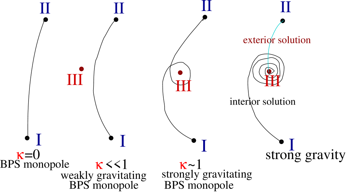
Global solutions of Eqs.(16) can then be viewed as trajectories in the phase space interpolating between fixed point I (origin) and fixed point II (infinity). Their behavior is schematically sketched in Fig.2. For the 4D solution is the flat space BPS monopole and its 5D analog is the flat space YM vortex. For the solution is a weakly gravitating 5D vortex whose field configuration is only slightly deformed as compared to the case. The YM vortices therefore do generalize to curved space, unlike the YM particles.
5.1 Strong gravity limit
Further increasing the gravitational coupling deforms the YM vortex more and more and the phase space trajectory approaches closer and closer the third fixed point.


Since the latter has complex eigenvalues with negative real part, the phase trajectory gets attracted by this fixed point and oscillates around it for a while before going to infinity. These oscillations manifest themselves in the solution profiles; see Fig.3. A further increase of the gravitational force is not accompanied by an increase of the value of but can rather be achieved by increasing the value of . The parameters , , etc. then start developing spiraling oscillations around some limiting values; see Fig.3.
Such strongly gravitating solutions have a regular core connected to the asymptotic region by a long throat – the region where the radius of the two-sphere, , is approximately constant and all other field amplitudes oscillate around the constant values (20). Increasing the value of this throat becomes longer and longer, and finally the solution splits up into the two independent solutions: interior and exterior, schematically shown in Fig.4.


The interior solution has a regular central core and approaches asymptotically the ‘warped ADS’ geometry (21). In Fig.2 this solution corresponds to the phase trajectory that starts at the fixed point I and after infinitely many oscillations around the fixed point III ends up there. The exterior solution, shown in Fig.4, interpolates between the ‘warped ADS’ and infinity. In Fig.2 this solution corresponds to the phase trajectory that interpolates between the fixed points III and II. It does not oscillate, since all ‘repelling’ eigenvalues (22) with positive real part are real. This solution is somewhat similar to an extreme non-Abelian black string, since passing to the Schwarzschild gauge where one has
where the event horizon radius is .
5.2 Conclusions
Summarizing the above discussion, although the static and SO(4) symmetric YM particles in D=5 get destroyed by gravity, in view of their scaling behavior, the static and SO(3) symmetric solutions – YM vortices – do admit non-trivial curved space generalizations, since their scale invariance is broken by the asymptotic value of the ‘Higgs field’ . These gravitating YM vortices comprise a one-parameter family of globally regular solutions – the fundamental branch – that interpolates between the flat space BPS monopole and the extreme non-Abelian black string. For all these solutions the YM field amplitude is positive definite. In addition, there exist also excitations over the fundamental branch. These are solutions for which the YM field amplitude oscillates around zero value, these solutions do not have the flat space limit.
6 Generalized YM vortices
The gravitating YM vortex solutions of the fundamental branch (but not the excited ones) have been generalized in a number of ways.
6.1 YM black strings [29]
From the 4D viewpoint the YM vortices are regular gravitating solitons. It has been known for quite a long time [28] that gravitating solitons can often be generalized to include a small black hole in the center. Technically this requires replacing the boundary conditions at the regular origin (conditions of the type (10)) by the boundary conditions at the regular event horizon (conditions of the type (11)). Such a procedure has been used [29] to promote the regular YM vortices to black strings.
For a given there can be several YM vortex solutions corresponding to different parts of the spiraling curves in Fig.3. This property generalizes also to the black string case, where one also finds several black string solutions for a given , provided that their even horizon radius is small enough. As increases, these solutions approach each other and finally merge for some maximal value . There are no black strings with , and so black strings exist only in a finite domain of the parameter plane. Black strings and regular vortex solutions with a -term [30, 31] have also been considered.
6.2 ‘Twisted’ solutions [32, 33]
When performing the dimensional reduction from D=5 to D=4 in Eqs.(14) and (5) it was assumed that the Killing vector is hypersurface orthogonal. Relaxing this condition, Eq.(14) generalizes to
where the twist can be viewed as a 4D vector field. Inserting this to the action (4) gives instead of (5) a four dimensional EYM-Higgs-dilaton+U(1) model. The solutions of this ‘twisted’ model carry an additional U(1) charge under the vector field . This charge can be of electric [32] or magnetic [33] type. When this charge vanishes, the solutions reduce to the YM vortices/black strings.
6.3 Deformed and stationary solutions [34, 35, 36]
The 5D YM vortices/black strings, with or without twist, have been also generalized [34, 35, 36] to the case where, after the dimensional reduction to D=4, the fields are chosen to be static and axially symmetric, rather than spherically symmetric. The ansatz for the gauge field and contains in this case two integer winding numbers, . If then the solutions are spherically symmetric monopoles. For , one obtains axially symmetric solutions of the multimonopole type. Solutions with describe monopole-antimonopole pairs. Both regular solutions [35] and black strings [36] have been considered within this approach. In all cases the existence of several solutions for a given value of has been detected.
6.4 Non-Abelian braneworlds [37, 39, 40, 41, 42]
Solutions with gravitating gauge fields can also be considered in the context of the braneworld models. As was discussed above, the non-Abelian monopole describes a one-dimensional object (vortex) in D=5. It will therefore describe a two-dimensional object (domain wall) in D=6 and a three-dimensional object (3-brane) in D=7. In all cases the SU(2) Yang-Mills field and the triplet Higgs fields can be chosen to be static and spherically symmetric,
| (23) |
with . For the 3-brane in D=7 one chooses to be coordinates orthogonal to the brane, the 7D metric being
| (24) |
where are coordinates on the brane. Integrating the coupled EYM-Higgs- equations reveals [37] that there are solutions satisfying the regularity condition at the brane, , , for which for . Such solutions describe globally regular braneworlds confined in the monopole core with gravity localized on it. Solitonic braneworlds have also been studied in systems with a gravitating global monopole [38] and also for the local and global monopoles [39] coupled to each other and to gravity in D=7.
More general solutions of the -brane type have been obtained [40, 41, 42] by oxidizing the YM vortices to dimensions. The metric is then chosen to be
| (25) |
with the gauge field given by
| (26) |
What is interesting, the analog of the fixed point (19) can be obtained [40] within this approach for any , also expressed in terms of roots of a cubic polynomial.
7 Non-Abelian solitons in string theory
Coming to the question of why one should study gravitating Yang-Mills fields in higher dimensions, one can say that (apart form pure curiosity) the motivation for this is provided by string theory. Gravitating Yang-Mills fields enter supersymmetry multiplets of the supergravity (SUGRA) theories to which string theory reduces at low energies. The knowledge of the basic solutions for gravitating gauge fields can therefore be useful for constructing solutions in low energy string theory. However, unlike solutions of the pure vacuum gravity, solutions of the EYM theory will not directly solve equations of SUGRA, since the latter generically contain additional fields, as for example the dilaton field. Constructing supergravity solutions with Yang-Mills fields is thus more complicated. However, imposing the supersymmetry conditions one can sometimes reduce the problem to solving first order Bogomol’nyi equations and not the second order field equations.
7.1 Heterotic solitons [43, 44]
The first example of supersymmetric solutions with gravitating Yang-Mills fields was obtained by Strominger [43] in the heterotic string theory. The low energy limit of the latter is a supergravity whose bosonic sector contains a Yang-Mills field already in D=10. Strominger considers a 5-brane in D=10 and makes the 6+4 split of the metric,
where // are coordinates on the brane while the coordinated of the 4-space orthogonal to the brane are /. He puts the Yang-Mills field to the orthogonal Euclidean 4-space,
Since the Yang-Mills field in D=4 is conformally invariant and the relevant 4D part of the metric is conformally flat, the scale factor drops out from the Yang-Mills equations. As a result, any flat space self-dual Yang-Mills instanton in D=4,
| (27) |
will solve the Yang-Mills part of the SUGRA equations. The metric functions as well as the axion and dilaton will then satisfy the Poisson equation on with the source determined by , and so the solution can be expressed in quadratures. As there are many solutions of Eqs.(27), this gives a large family of heterotic 5-branes in D=10. Performing then dimensional reductions, one can construct [44] yet many more different solutions living in . All these are called heterotic solitons.
7.2 Non-Abelian vacua in gauged SUGRAs [48, 50, 51, 55, 57, 58]
Type I and type II string theories and also M theory reduce at low energies to supergravities in D=10 and D=11 whose multiplets do not contain Yang-Mills fields. However, the latter appear when one performs dimensional reductions on internal manifolds with non-Abelian isometries. This gives gauged SUGRAs in lower dimensions whose gauge group is related to the isometry group of the internal manifold. For example, the reduction of type II string theory on gives the gauged SUGRA in D=5 whose solutions are used in the AdS/CFT correspondence. Another example is the reduction of M theory on , which gives [45] the N=8 gauged SUGRA in D=4 with the local SO(8)SU(8) invariance. One can then study solutions in these SUGRAs, and lifting them back to will give vacua of string or M theory.
The field content of a gauged SUGRA model can be quite complicated, which is why the gauge fields are often set to zero to find solutions. This gives, for example, black holes with scalar hair [46, 47] in N=8 SUGRA. However, in some cases one can construct solutions also with gravitating gauge fields. Let us consider a SUGRA model [48] in D=4 which is a consistent truncation of the maximal N=8 SUGRA,
| (28) |
This theory contains a gravity-coupled Yang-Mills field with gauge group SU(2) and the dilaton, whose potential depends on a real parameter . In the static and spherically symmetric case the fields are given by
For one-shell configurations the amplitudes satisfy a system of second order ODEs whose solutions can be studied [49] numerically. Instead of solving these equations, one can also consider the conditions for the fields to have unbroken supersymmetries. These conditions require the existence of a non-trivial spinor satisfying the linear equations
| (29) |
where . In general these equations are inconsistent, since there are 80 equations for 16 components of , and so the only solution is . However, one can show [48] that if the background fields are such that the following conditions are fulfilled,
| (30) |
where is a constant and
then there exist four independent solutions of Eqs.(29), which corresponds to the N=1 supersymmetry.


Solutions [48] of the Bogomol’nyi equations (7.2) with the regular boundary condition at the origin, , comprise a continuous family labeled by and show three completely different types of behavior, depending on the sign on . For the dilaton is everywhere bounded and the solutions approach the AdS metric in the asymptotic region. For the solutions are of the ‘bag of gold’ type, since they have compact spatial sections with the topology of . The geometry is generically singular at one pole of the . However, for the solution is globally regular, the dilaton is constant, the geometry is that of , and the gauge field potential coincides with the invariant forms on . All these solutions can be uplifted [48] to to become vacua of M theory.
For the solution is given by [50]
| (31) |
This solution can be uplifted [51] to D=10, the string frame metric and the three-form in D=10 then being given by
| (32) |
where is the gauge field 2-form and with being the invariant forms on . This solution describes a 3-brane in D=10.
This solution was originally obtained [50, 51] by Chamseddine and Volkov, both in D=4 and D=10. A very interesting holographic interpretation for this solution was then proposed [52] by Maldacena and Nunez, according to which this solution describes the NS-NS 5-brane wrapped on , in which case it effectively becomes a 3-brane. As a result, the solution provides a dual SUGRA description for the wrapped brane worldvolume theory, which is the (deformed) N=1 Super Yang-Mills in D=4. Since this theory is confining, one can say that the solution (31),(32) provides the dual SUGRA description for the phenomenon of confinement. For example, the value of the Wilson loop, the beta-function and other parameters of the confining gauge field theory can be obtained by simply computing some purely geometrical parameters of the solution, like areas of spheres and the values of the -fluxes through them. As a result, this solution with self-gravitating Yang-Mills field has found quite interesting and serious applications. Generally known as solution of Maldacena and Nunez (the names of Chamseddine and Volkov seem now to be completely forgotten) it plays an important role in the analysis of string theory (see [53, 54] for recent reviews).
Non Abelian vacua have also been studied [55] in the context of a gauged SUGRA in D=5. The gravitational and gauge fields in this case are given by the same SO(4) invariant expressions (5) as for the YM particle, and there are also the dilaton and axion. The solutions are not asymptotically flat, they have two supercharges, and they can be used [56] for a dual SUGRA description of the confining N=1 Super-Yang-Mills theory in D=3.
The discussed above supersymmetric solutions [50, 55] have also been generalized [57, 58] to the case where the spatial part of the metric is , where is a maximal symmetry space, that is sphere, hyperboloid or Euclidean space. Their black hole generalizations [59, 60] have been used for a holographic description of the confinement/deconfinement phase transition in the dual gauge theory.
References
- [1] A. Lichenrowitcz, Théories Relativistes de la Gravitation et de l’Electromagnétisme (Masson, Paris, 1955).
- [2] S. Deser, Absence of static solutions in source-free Yang-Mills theory. Phys.Lett. B 64, 463 (1976).
- [3] S. Coleman, There are no classical glueballs. Comm.Math.Phys. 55, 113 (1977).
- [4] S. Coleman and L. Smarr, Are there geon analogs in sourceless gauge field theories ? Comm.Math.Phys. 56, 1 (1977).
- [5] R. Bartnik and J. McKinnon, Particlelike solutions of the Einstein-Yang-Mills equations. Phys.Rev.Lett. 61, 141 (1988).
- [6] M.S. Volkov and D.V. Gal’tsov, Non-Abelian Einstein-Yang-Mills black holes. JETP Lett. 50, 346 (1989).
- [7] H. Kunzle and A.K.M. Masood ul Alam, Spherically symmetric static SU(2) Einstein-Yang-Mills fields. J.Math.Phys. 31, 928 (1990).
- [8] P. Bizon, Colored black holes. Phys.Rev.Lett. 64, 2844 (1990).
- [9] R. Ruffini and J.A. Wheeler, Introducing the black hole. Phys. Today 24, 30 (1971).
- [10] B. Kleihaus and J. Kunz, Static axially symmetric solutions of Einstein Yang-Mills dilaton theory. Phys.Rev.Lett. 78, 2527 (1997); [arXiv: hep-th/9612101].
- [11] B. Kleihaus and J. Kunz, Static black hole solutions with axial symmetry. Phys.Rev.Lett. 79, 1595 (1997); [arXiv: gr-qc/9704060].
- [12] B. Kleihaus and J. Kunz, Rotating hairy black holes. Phys.Rev.Lett. 86, 3704 (2001); [arXiv: gr-qc/0012081].
- [13] M.S. Volkov and D.V. Gal’tsov, Gravitating non-Abelian solitons and black holes with Yang-Mills fields. Phys.Rep. 319, 1 (1999); [arXiv: hep-th/9810070].
- [14] R. Emparan and H.S. Reall, Black rings. Class.Quant.Grav. 23, R169 (2006); [arXiv: hep-th/0608012].
- [15] T. Eguchi, P.B. Gilkey and A.J. Hanson, Gravitation, gauge theories and differential geometry. Phys.Rep. 66, 213 (1980).
- [16] A.A. Belavin, A. M. Polyakov, A.S. Shvarts, Yu.S. Tyupkin, Pseudoparticle solutions of the Yang-Mills equations. Phys.Lett. B59, 85 (1975).
- [17] E.B. Bogomol’nyi, Stability of classical solutions. Sov.J.Nucl.Phys. 24, 676 (1976).
- [18] M.S. Volkov, Gravitating Yang-Mills vortices in 4+1 spacetime dimensions. Phys. Lett. B524, 369 (2002); [arXiv: hep-th/0103038].
- [19] Y. Brihaye, A.Chakrabarti and D.H. Tchrakian, Particle-like solutions to higher order curvature Einstein-Yang-Mills systems in d-dimensions. Class.Quant.Grav. 20, 2765 (2003); [arXiv: hep-th/0202141].
- [20] N. Okuyama and Kei-ichi-Maeda, Five-dimensional black hole and particle solution with non-Abelian gauge field. Phys. Rev. D 67, 104012 (2003); [arXiv: hep-th/0212022].
- [21] Y. Brihaye, A.Chakrabarti, B. Hartmann and D.H. Tchrakian, Higher order curvature generalizations of Bartnick-McKinnon and colored black hole solutions in D = 5. Phys.Lett. B 561, 161 (2003);[arXiv: hep-th/0212288].
- [22] E. Radu and D.H. Tchrakian, No hair conjecture, non-Abelian hierarchies and Anti-de Sitter spacetime. Phys.Rev. D 73, 024006 (2006); [arXiv: gr-qc/0508033].
- [23] E. Radu, C. Stelea and D.H. Tchrakian, Features of gravity-Yang-Mills hierarchies in d-dimensions. Phys.Rev. D 73, 084015 (2006); [arXiv: gr-qc/0601098].
- [24] Y. Brihaye, E. Radu and D.H. Tchrakian, Einstein-Yang-Mills solutions in higher dimensional de Sitter spacetime. [arXiv: gr-qc/0610087].
- [25] P. Breitenlihner, D. Maison and D.H. Tchrakian, Regular solutions to higher order curvature Einstein-Yang-Mills systems in higher dimensions. Class.Quant.Grav. 22, 5201 (2005); [arXiv: gr-qc/0508027].
- [26] E. Radu, Ya. Shnir and D.H. Tchrakian, Particle-like solutions to the Yang-Mills-dilaton system in d=4+1 dimensions. [arXiv: hep-th/0611270].
- [27] G.W. Gibbons and P. Townsend, Self-gravitating Yang monopoles in all dimensions. Class.Quant.Grav. 23, 4873 (2006); [arXiv: hep-th/0604024].
- [28] D. Kastor, J.H. Traschen, Horizon inside classical lumps. Phys.Rev. D 46, 5399 (1992); [arXiv: hep-th/9207070].
- [29] B. Hartmann, Non-Abelian black strings. Phys.Lett. B 602, 231 (2004); [arXiv: hep-th/0409006].
- [30] F. Bakkalo Taheri and Y. Brihaye, Non-Abelian black strings and cosmological constant. [arXiv: gr-qc/0605040].
- [31] Y. Brihaye and T. Delsate, Black strings and solitons in five dimensional space-time with positive cosmological constant. [arXiv: hep-th/0611195].
- [32] Y. Brihaye and E. Radu, Gravitating Yang-Mills dyon vortices in 4+1 spacetime dimensions. Phys.Lett. B 605, 190 (2005); [arXiv: hep-th/0409065].
- [33] Y. Brihaye and E. Radu, Kaluza-Klein black holes with squashed horizons and d=4 superposed monopoles. Phys.Lett. B 641, 212 (2006); [arXiv: hep-th/0606228].
- [34] Y. Brihaye, B. Hartmann, Dilatonic monopoles from (4+1)-dimensional vortices. Phys.Lett. B 534, 137 (2002); [arXiv: hep-th/0202054].
- [35] Y. Brihaye, B. Hartmann and E. Radu, Deformed vortices in (4+1)-dimensional Einstein - Yang - Mills theory. Phys.Rev. D 71, 085002 (2005). [arXiv: hep-th/0502131].
- [36] Y. Brihaye, B. Hartmann and E. Radu, Black strings in (4+1)-dimensional Einstein-Yang-Mills theory. Phys.Rev. D 72, 104008 (2005); [arXiv: hep-th/0508028].
- [37] E. Roessl and M. Shaposhnikov, Localizing gravity on a ’t Hooft-Polyakov monopole in seven-dimensions. Phys.Rev. D 66, 084008 (2002); [arXiv: hep-th/0205320].
- [38] T. Gherghetta, E. Roessl and M. Shaposhnikov, Living inside a hedgehog: Higher dimensional solutions that localize gravity. Phys.Lett. B 491, 353 (2000); [arXiv: hep-th/0006251].
- [39] E. R. Bezerra de Mello and B. Hartmann, Localizing gravity in composite monopole brane worlds without bulk cosmological constant. Phys.Lett. B 639, 546 (2006); [arXiv: hep-th/0603077].
- [40] Y. Brihaye, F. Clement, B. Hartmann, Spherically symmetric Yang-Mills solutions in a (4+n)-dimensional space-time. Phys.Rev. D 70, 084003 (2004); [arXiv: hep-th/0403041].
- [41] Y. Brihaye, B. Hartmann, Spherically symmetric solutions of a (4+n) - dimensional Einstein-Yang-Mills model with cosmological constant. Class.Quant.Grav. 22, 183 (2005); [arXiv: hep-th/0403296].
- [42] B. Hartmann, Y. Brihaye, B. Bertrand, Spherically symmetric Yang-Mills solutions in a five-dimensional anti-de Sitter space-time. Phys.Lett. B 570, 137 (2003); [arXiv: hep-th/0307065].
- [43] A. Strominger, Heterotic solitons. Nucl.Phys. B 343, 167 (1990).
- [44] M.J. Duff, R.R. Khuri and J.X. Lu, String solitons. Phys.Rep. 259, 213 (1995); [arXiv: hep-th/9412184].
- [45] B. de Wit and H. Nicolai, N=8 Supergravity. Nucl.Phys. B 208, 323 (1982).
- [46] M.J. Duff and J.T. Liu, Anti-de Sitter black holes in gauged N = 8 supergravity. Nucl.Phys. B 554, 237 (1999); [arXiv: hep-th/9901149].
- [47] T. Hertog and K. Maeda, Black holes with scalar hair and asymptotics in N = 8 supergravity. JHEP 0407: 051 (2004); [arXiv: hep-th/0404261].
- [48] A. Chamseddine and M.S. Volkov, Non-Abelian solitons in N=4 gauged supergravity and leading order string theory. Phys.Rev. D 70, 086007 (2004); [arXiv: hep-th/0404171].
- [49] R.B. Mann, E. Radu and D.H. Tchrakian, Non-Abelian solutions in AdS(4) and d=11 supergravity. Phys.Rev. D 74, 064015 (2006); [arXiv: hep-th/0606004].
- [50] A. Chamseddine and M.S. Volkov, Regular non-Abelian vacua in N = 4, SO(4) gauged supergravity. Phys.Rev.Lett. 79, 3343 (1997); [arXiv: hep-th/9711181].
- [51] A. Chamseddine and M.S. Volkov, Non-Abelian BPS monopoles in N=4 gauged supergravity. Phys.Rev. D 57, 6242 (1998); [arXiv: hep-th/9707176].
- [52] J.M. Maldacena and C. Nunez, Towards the large N limit of pure N=1 super-Yang-Mills. Phys.Rev.Lett. 86, 588 (2001); [arXiv: hep-th/0008001].
- [53] M. Grana, Flux compactifications in string theory: A Comprehensive review. Phys.Rep. 423, 91 (2006); [arXiv: hep-th/0509003].
- [54] J.D. Edelstein, R. Portugues, Gauge/string duality in confining theories. Fortsch.Phys. 54, 525 (2006); [arXiv: hep-th/0602021].
- [55] A. Chamseddine and M.S. Volkov, Non-Abelian vacua in D = 5, N=4 gauged supergravity. JHEP 0104, 023 (2001); [arXiv: hep-th/0101202].
- [56] J.M. Maldacena and H. Nastase, The Supergravity dual of a theory with dynamical supersymmetry breaking. JHEP 0109, 024 (2001); [arXiv: hep-th/0105049].
- [57] E. Radu, New non-Abelian solutions in D = 4, N=4 gauged supergravity. Phys.Lett. B 542, 275 (2002); [arXiv: gr-qc/0202103].
- [58] E. Radu, Non-Abelian solutions in N=4, D=5 gauged supergravity. Class.Quant.Grav. 23, 4369 (2006); [arXiv: hep-th/0601135].
- [59] S.S. Gubser, A.A. Tseytlin and M.S. Volkov, Non-Abelian 4-d black holes, wrapped five-branes, and their dual descriptions. JHEP 0109, 017 (2001); [arXiv: hep-th/0108205].
- [60] G. Bertoldi, 5-D black holes, wrapped fivebranes and 3-D Chern-Simons super Yang-Mills. JHEP 0210, 042 (2002); [arXiv: hep-th/0210048].