$1/R$ multidimensional gravity with form-fields: stabilization of extra dimensions, cosmic acceleration and domain walls

Abstract

We study multidimensional gravitational models with scalar curvature nonlinearity of the type $1/R$ and with form-fields (fluxes) as a matter source. It is assumed that the higher dimensional space-time undergoes Freund-Rubin-like spontaneous compactification to a warped product manifold. It is shown that for certain parameter regions the model allows for a freezing stabilization of the internal space near the positive minimum of the effective potential which plays the role of the positive cosmological constant. This cosmological constant provides the observable late-time accelerating expansion of the Universe if parameters of the model is fine tuned. Additionally, the effective potential has the saddle point. It results in domain walls in the Universe. We show that these domain walls do not undergo inflation.

I Introduction

There are two great challenges in modern theoretical physics and cosmology. The first big puzzle consists in a ”dark side” of our Universe. Recent observations of the luminosity distances of type Ia supernovas (SNIa), CMB angular temperature fluctuations on degree scales, and measurements of the power spectrum of galaxy clustering indicate (see e.g. WMAP2006 ) that our Universe spatially flat with $\sim 23\%$ of its critical energy in non-relativistic cold dark matter and $\sim 73\%$ in a smooth component having a large negative pressure (dark energy). The latter one results in accelerating expansion of our Universe which began approximately at redshift $z\sim 1$ and continues until present time. On the other hand, there is also possibility that the late-time accelerating expansion of our Universe is caused by modification of gravity on Galactic scales. For example, it was proposed R^-1 to add a $1/R$ term in the Einstein-Hilbert action to modify General Relativity. It is clear that such modification may affect dynamics of the Universe at late times of its evolution and on large scales where the scalar curvature becomes small. In fact, it was shown (see e.g. Carroll ) that this term can provide accelerating expansion of the Universe without the need of introducing dark energy.

The second great challenge is possible multidimensionality of our Universe which naturally follows from theories unifying different fundamental interactions with gravity, such as string/M-theory. So, there is big temptation to explain the dark matter and the accelerating expansion of our Universe with the help of extra dimensions. However, it is well known that dynamical behavior of internal spaces usually results in variations of the effective four-dimensional fundamental ”constants” (e.g. gravitational constant, fine structure constant, etc.) (see e.g. Zhuk(IJMP) -Alimi ) and references therein). There are strong experimental bounds on such variations Uzan . So, one of the main problems of higher-dimensional models lies in stable compactification of the internal spaces. Scale factors of the internal spaces play the role of scalar fields moving in our four-dimensional space-time. Their dynamics is defined by an effective potential in dimensionally reduced theory. Thus, the internal spaces are stabilized in the case of a minimum of this potential GZ(PRD1997) . Small excitations around this minimum look in our Universe as massive scalar fields (gravitational excitons/radions GZ(PRD1997) ) with Planck scale suppression of their interaction with usual matter GSZ . Therefore they may play the role of dark matter. Additionally, if the minimum of the effective potential is positive, it contributes in positive cosmological constant providing acceleration of the Universe.

In the present paper, we consider nonlinear gravitational multidimensional cosmological model with action of the type $R+1/R$ with form-fields as a matter source. We also include a bare cosmological term as an additional parameter of the theory. It is assumed that the corresponding higher-dimensional space-time manifold undergos a spontaneous compactification to a manifold with warped product structure of the external and internal spaces. Each of spaces has its own scale factor. A model without form-fields and bare cosmological constant was considered in paper GZBR where the internal space freezing stabilization was achieved due to negative minimum of the effective potential. Thus, such model is asymptotically AdS without accelerating behavior of our Universe. It is well known that inclusion of usual matter can uplift potential to the positive values GMZ(PRDb) . One of the main task of our present investigations is to observe such uplifting due to the form-fields. Indeed, we demonstrate that for certain parameter regions the late-time acceleration scenario in our model becomes reachable. However, it is not simple uplifting of the negative minimum of the theory GZBR to the positive values. The presence of the form-fields results in much more rich structure of the effective potential then in GZBR . Here, we obtain additional branches with extremum points, and one of such extremum corresponds to the positive minimum of the effective potential. This minimum plays the role of the positive cosmological constant. With the corresponding fine tuning of the parameters, it can provide the late-time accelerating expansion of the Universe. Moreover, we show that for this branch of the effective potential there is also a saddle point. Thus, we obtain domain walls which separate regions with different vacua. We demonstrate that these domain walls do not undergo inflation because our effective potential is not flat enough around the saddle point.

It is also worth of noting that the effective potential in our reduced model has a branchpoint. It gives very interesting possibility to investigate transitions from one branch to another by analogy with catastrophe theory or similar to phase transitions in statistical theory. This idea needs more detail investigation in a separate paper.

The paper is structured as follows. In section II we present a brief description of multidimensional models with scalar curvature nonlinearity $f(R)$ and the form-fields as a matter source. Then, we perform dimensional reduction and obtain effective four-dimensional action with effective potential. General formulas from this section are applied to our specific model $f({R})={R}-\mu/{R}-2\Lambda_{D}$ in section III. Here, we obtain the effective potential minimum conditions. These conditions are analyzed in sections IV and V for the cases of zero and positive effective cosmological constants respectively. Furthermore, in section VI we demonstrate that the positive minimum of the effective potential plays the role of the positive cosmological constant and can provide the late-time accelerating expansion. Additionally, this minimum is accompanied by a saddle point. It results in non-inflating domain walls in the Universe. The main results are summarized and discussed in the concluding section VII.

II General setup

We consider a $D=(D_{0}+D^{\prime})-$dimensional nonlinear gravitational theory with action functional

$$S = \frac{1}{2\kappa^{2}_{D}}\int_{M}d^{D}x\sqrt{|\bar{g}|}f(\bar{R})$$ (2.1)

$$- \frac{1}{2}\int_{M}d^{D}x\sqrt{|\bar{g}|}\sum^{n}_{i=1}\frac{1}{d_{i}!}\left(F^{(i)}\right)^{2}\,,$$

where $f(\bar{R})$ is an arbitrary smooth function of a scalar curvature $\bar{R}:=R[\bar{g}]$ constructed from the $D-$dimensional metric $\bar{g}_{ab}\;(a,b=1,\ldots,D)$. $D^{\prime}$ is the number of extra dimensions. $\kappa^{2}_{D}$ denotes the $D-$dimensional gravitational constant. In action (2.1), a form field (flux) $F$ has block-orthogonal structure consisting of $n$ blocks. Each of these blocks is described by its own antisymmetric tensor field $F^{(i)}(i=1,\ldots,n)$ of rank $d_{i}$ ($d_{i}$-form field strength). Additionally, we assume that for the sum of the ranks holds $\sum^{n}_{i=1}d_{i}=D^{\prime}$.

Following Refs. GZBR -GMZ(ASS) , we can show that the nonlinear gravitational theory (2.1) is equivalent to a linear theory $R=R[g]$ with conformally transformed metric

$$g_{ab}=\Omega^{2}\bar{g}_{ab}=\left[f^{\prime}(\bar{R})\right]^{2/(D-2)}\bar{g}_{ab}\;$$ (2.2)

and an additional minimal scalar field $\phi=\ln[f^{\prime}(\bar{R})]/A$ coupled with fluxes. The scalar field $\phi$ is the result and the carrier of the curvature nonlinearity of the original theory. Thus, for brevity, we shall refer to the field $\phi$ as nonlinearity scalar field. A self-interaction potential $U(\phi)$ of the scalar field $\phi$ reads

$$U(\phi)=\frac{1}{2}e^{-B\phi}\left[\;\bar{R}(\phi)e^{A\phi}-f\left(\bar{R}(\phi)\right)\right]\;,$$ (2.3)

where

$$A=\sqrt{\frac{D-2}{D-1}}\,,\quad B=\frac{D}{\sqrt{(D-2)(D-1)}}\,.$$ (2.4)

Furthermore, we assume that the multidimensional space-time manifold undergoes a spontaneous compactification

$$M\longrightarrow M=M_{0}\times M_{1}\times\ldots\times M_{n}$$ (2.5)

in accordance with the block-orthogonal structure of the field strength $F$, and that the form fields $F^{(i)}$, each nested in its own $d_{i}-$dimensional factor space $M_{i}\,(i=1,\ldots,n)$, respect a generalized Freund-Rubin ansatz FR . Here, ($D_{0}=4$)-dimensional space-time $M_{0}$ is treated as our external Universe with metric $g^{(0)}(x)$.

This allows us to perform a dimensional reduction of our model along the lines of Refs. GZ(PRD1997) -GMZ(PRDa) ,GZ(PRD2000) ,RZ . The factor spaces $M_{i}$ are then Einstein spaces with metrics $g^{(i)}\equiv e^{2\beta^{i}(x)}\gamma^{(i)}$ which depend only through the warp factors $a_{i}(x):=e^{\beta^{i}(x)}$ on the coordinates $x$ of the external space-time $M_{0}$. For the corresponding scalar curvatures holds $R\left[\gamma^{(i)}\right]=\lambda^{i}d_{i}\equiv r_{i}$ (in the case of the constant curvature spaces $\lambda^{i}=k_{i}(d_{i}-1),\,\,k_{i}=0,\pm 1$). The warped product of Einstein spaces leads to a scalar curvature $\bar{R}$ which depends only on the coordinate $x$ of the $D_{0}-$dimensional external space-time $M_{0}$: $\bar{R}[\bar{g}]=\bar{R}(x)$. This implies that the nonlinearity field $\phi$ is also a function only of $x$: $\phi=\phi(x)$. Additionally, it can be easily seen GZBR that the generalized Freund-Rubin ansatz results in the following expression for the form-fields: $\left(F^{(i)}\right)^{2}=f_{i}^{2}/a_{i}^{2d_{i}}$ where $f^{i}=const$.

In general, the model will allow for several stable scale factor configurations (minima in the landscape over the space of volume moduli). We choose one of them (which we expect to correspond to current evolution stage of our observable Universe), denote the corresponding scale factors as $\beta^{i}_{0}$, and work further on with the deviations $\hat{\beta}^{i}(x)=\beta^{i}(x)-\beta^{i}_{0}$.

Without loss of generality, we shall consider a model with only one $d_{1}$-dimensional internal space. After dimensional reduction and subsequent conformal transformation to the Einstein frame the action functional (2.1) reads

$$S = \frac{1}{2\kappa_{0}^{2}}\int\limits_{M_{0}}d^{D_{0}}x\sqrt{|\tilde{g}^{(0)}|}\left\{R\left[\tilde{g}^{(0)}\right]-\tilde{g}^{(0)\mu\nu}\partial_{\mu}\varphi\partial_{\nu}\varphi\right.$$ (2.6)

$$- \left.\tilde{g}^{(0)\mu\nu}\partial_{\mu}\phi\partial_{\nu}\phi-2U_{eff}(\varphi,\phi)\right\}\,,$$

where $\varphi:=-\sqrt{d_{1}(D-2)/(D_{0}-2)}\,\hat{\beta}^{1}$ and $\kappa^{2}_{0}:=\kappa^{2}_{D}/V_{d_{1}}$ denotes the $D_{0}-$dimensional (four-dimensional) gravitational constant. $V_{d_{1}}\sim\exp{(d_{1}\beta_{0}^{1})}$ is the volume of the internal space at the present time.

A stable compactification of the internal space $M_{1}$ is ensured when its scale factor $\varphi$ is frozen at the minimum of the effective potential

$$U_{eff}=e^{b\varphi}\left[-\frac{1}{2}R_{1}e^{a\varphi}+U(\phi)+he^{c\phi}e^{ad_{1}\varphi}\right]\,,$$ (2.7)

where $R_{1}:=r_{1}\exp{(-2\beta^{1}_{0})}$ defines the curvature of the internal space at the present time and contribution of the form-field into the effective action is described by $h:=\kappa^{2}_{D}\,f^{2}_{1}\exp{(-2d_{1}\beta^{1}_{0})}>0$. For brevity we introduce notations

$$a: = 2\sqrt{\frac{D_{0}-2}{d_{1}(D-2)}}\;,\;b:\;=2\sqrt{\frac{d_{1}}{(D-2)(D_{0}-2)}}\;,$$

$$c: = \frac{2d_{1}-D}{\sqrt{(D-1)(D-2)}}\;.$$ (2.8)

III The model

In this section we analyze the conditions of the compactification for a model with

$$f(\bar{R})=\bar{R}-\frac{\mu}{\bar{R}}-2\Lambda_{D}\;.$$ (3.1)

Then from the relation $f^{\prime}(\bar{R})=\exp{(A\phi)}$ we obtain

$$\bar{R}=q\sqrt{\frac{|\mu|}{s(e^{A\phi}-1)}}\;,\quad q=\pm 1\;,\,s=\mbox{\rm sign}\,(\mu)\;.$$ (3.2)

Thus, the ranges of variation of $\phi$ are $\phi\in(-\infty,0)$ for $\mu<0\;(s=-1)$ and $\phi\in(0,+\infty)$ for $\mu>0\;(s=+1)$.

It is worth of noting that the limit $\phi\to\pm 0\;(f^{\prime}\to 1)$ corresponds to the transition to a linear theory: $f(\bar{R})\to\bar{R}-2\Lambda_{D}$ and $R\to\bar{R}$. This is general feature of all nonlinear models $f(\bar{R})$. For example, in our case (3.1) we obtain $f(\bar{R})=\bar{R}\left(2-\exp(A\phi)\right)-2\Lambda_{D}\ \longrightarrow\bar{R}-2\Lambda_{D}$ for $\phi\to 0$. From other hand, for particular model (3.1), eq. (3.2) shows that the point $\phi=0$ maps into infinity $\bar{R},R=\pm\infty$. Thus, in this sense, we shall refer to the point $\phi=0$ as singularity.

For our model (3.1), potential (2.3) $U(\phi)$ reads

$$U(\phi)=\frac{1}{2}e^{-B\phi}\left(2qs\sqrt{|\mu|}\sqrt{se^{A\phi}-s}+2\Lambda_{D}\right)\,.$$ (3.3)

It is well known (see e.g. GMZ(PRDb) ,GMZ(PRDa) ,GZ(PRD2000) ) that in order to ensure a stabilization and asymptotical freezing of the internal space $M_{1}$, the effective potential (2.7) should have a minimum with respect to both scalar fields $\varphi$ and $\phi$. We remind that we choose the minimum position with respect to $\varphi$ at $\varphi=0$. Additionally, the eigenvalues of the mass matrix of the coupled $(\varphi,\phi)$-field system, i.e. the Hessian of the effective potential at the minimum position,

$$J:=\left.\left(\begin{array}[]{cc}\partial^{2}_{\varphi\varphi}U_{eff}&\partial^{2}_{\varphi\phi}U_{eff}\\ \\ \partial^{2}_{\phi\varphi}U_{eff}&\partial^{2}_{\phi\phi}U_{eff}\\ \end{array}\right)\right|_{extr}$$ (3.4)

should be positive definite (this condition ensures the positiveness of the mass squared of scalar field excitations). According to the Silvester criterion this is equivalent to the condition:

$$J_{11}>0\;,\quad J_{22}>0\;,\quad\mbox{det}(J)>0\quad.$$ (3.5)

It is convenient in further consideration to introduce the following notations:

$$\phi_{0}:=\phi|_{extr}\,,\,X:=\sqrt{se^{A\phi_{0}}-s}>0\,\rightarrow\,X_{(s=-1)}<1\,.$$ (3.6)

Then we can rewrite potentials $U(\phi)$, $U_{eff}(\varphi,\phi)$ and derivatives of the $U_{eff}$ at an extremum (possible minimum) position ($\varphi=0,\phi_{0}$) as follows:

$$U_{0}\equiv U|_{extr}=\left(1+sX^{2}\right)^{-B/A}\left(qs\sqrt{|\mu|}X+\Lambda_{D}\right),$$ (3.7)

$$U_{eff}|_{extr}=-\frac{1}{2}R_{1}+U_{0}(X)+h\left(1+sX^{2}\right)^{c/A}\;,$$ (3.8)

$$\partial_{\varphi}U_{eff}|_{extr} = -\frac{a+b}{2}R_{1}+bU_{0}(X)$$ (3.9)

$$+ (ad_{1}+b)h\left(1+sX^{2}\right)^{c/A}=0,\;\quad$$

$$\partial_{\phi}U_{eff}|_{extr} = ch\left(1+sX^{2}\right)^{c/A}-BU_{0}(X)$$ (3.10)

$$+ \frac{qA\sqrt{|\mu|}}{2X}\left(1+sX^{2}\right)^{1-B/A}=0,\qquad$$

$$\partial^{2}_{\varphi\varphi}U_{eff}|_{extr} = -\frac{(a+b)^{2}}{2}R_{1}+b^{2}U_{0}(X)$$ (3.11)

$$+ (ad_{1}+b)^{2}h\left(1+sX^{2}\right)^{c/A},\qquad$$

$$\partial^{2}_{\varphi\phi}U_{eff}|_{extr}=chad_{1}\left(1+sX^{2}\right)^{c/A}\;,$$ (3.12)

$$\partial^{2}_{\phi\phi}U_{eff}|_{extr} = ch\left(c-A+2B\right)\left(1+sX^{2}\right)^{c/A}$$ (3.13)

$$+ B(A-B)U_{0}(X)$$

$$- \frac{qs\sqrt{|\mu|}A^{2}}{4X^{3}}\left(1+sX^{2}\right)^{2-B/A}.\>\qquad$$

The most natural strategy for extracting detailed information about the location of stability region of parameters in which compactification is possible would consist in solving (3.10) for $X$ with subsequent back-substitution of the found roots into the inequalities (3.5) and the equation (3.9). To get the main features of the model under consideration, it is sufficient to investigate two particular nontrivial situations. Both of these cases are easy to handle analytically.

IV Zero effective cosmological constant: $\Lambda_{eff}=0$

It can be easily seen from eqs. (3.8) and (3.9) that condition $\Lambda_{eff}=U_{eff}|_{extr}=0$ results in relations

$$R_{1}=2d_{1}h\left(1+sX^{2}\right)^{c/A}=\frac{2d_{1}}{d_{1}-1}U_{0}(X)\;,\quad d_{1}\geq 2\;,$$ (4.1)

which enable us to get from eq. (3.10) quadratic equation for $X$

$$(d_{1}+1)X^{2}+qsd_{1}zX-s(d_{1}-1)=0\,,\quad z\equiv 2\Lambda_{D}/\sqrt{|\mu|}$$ (4.2)

with the following solutions:

$$X_{p} = qs\frac{d_{1}}{2(d_{1}+1)}\left(-z+p\>\sqrt{z^{2}+4s\frac{d^{2}_{1}-1}{d_{1}^{2}}}\right)\;,$$

$$p = \pm 1\,.$$ (4.3)

In the case $s=-1\;$ parameter $z$ should satisfy condition $|z|\geq z_{0}\equiv 2\sqrt{d_{1}^{2}-1}/d_{1}<2$ and for $z=z_{0}$ two solutions $X_{p}$ degenerate into one: $X_{p}\equiv X_{0}=-qs\sqrt{(d_{1}-1)/(d_{1}+1)}$.

Because of conditions $h\geq 0$ and $e^{A\phi_{0}}=1+sX^{2}>0$, the relations (4.1) show that parameters $R_{1}$ and $U_{0}(X)$ should be non-negative: $R_{1}\geq 0,\;U_{0}(X)\geq 0$. Obviously, only one of the solutions (IV) corresponds to a minimum of the effective potential. With respect to this solution we define parameters in the relation (4.1). Therefore, we must distinguish now which of $X_{p}$ corresponds to the minimum of $U_{eff}$. Let us investigate solutions (IV) for the purpose of their satisfactions to conditions $e^{A\phi_{0}}>0,\,U_{0}(X)\geq 0$ and $X_{p}\geq 0$.

The condition $e^{A\phi_{0}}=1+sX_{p}^{2}>0$:

Simple analysis shows that solutions $X_{p}$ satisfy this inequality for the following combinations of parameters:

$$\begin{array}[]{c}\mu>0\\ (s=+1)\end{array}$$

(4.4)

The condition $U_{0}(X)\geq 0$:

As appears from eq. (3.7), this condition takes place if $X_{p}$ satisfies inequality $2qsX_{p}+z\geq 0$ which leads to the conditions:

$$\begin{array}[]{c}\mu>0\\ (s=+1)\end{array}$$

(4.5)

The condition $X_{p}>0$:

This condition is satisfied for the combinations:

$$\begin{array}[]{c}\mu>0\\ (s=+1)\end{array}$$

(4.6)

The comparison of (4.4), (4.5) and (4.6) shows that they are simultaneously satisfied only for the following combinations:

$$\begin{array}[]{c}\mu>0\\ (s=+1)\end{array}$$

(4.7)

Additionally, the extremum solutions $X_{p}$ should correspond to the minimum of $U_{eff}$. The inequalities (3.5) are the sufficient and necessary conditions for that. We analyze them in the case of four-dimensional external space $D_{0}=4$. Taking into account definitions (2.4), (II), (3.11)-(3.13) and relations (4.1), for $J_{11},J_{22}$ and $J_{21}$ we get respectively:

$$J_{11}=\frac{8}{d_{1}+2}U_{0}(X_{p})\,,$$ (4.8)

$$\begin{split}J_{22}=&-\sqrt{|\mu|}\left[\frac{6d_{1}(2qsX_{p}+z)\left(1+sX_{p}^{2}\right)^{-\frac{d_{1}+4}{d_{1}+2}}}{(d_{1}-1)(d_{1}+2)(d_{1}+3)}\right.\\ &+\left.\frac{qs(d_{1}+2)}{4X^{3}_{p}(d_{1}+3)}\left(1+sX_{p}^{2}\right)^{\frac{d_{1}}{d_{1}+2}}\right]\,,\end{split}$$ (4.9)

$$J_{21}= - \sqrt{|\mu|}\left[\frac{(d_{1}-4)(2qsX_{p}+z)}{(d_{1}-1)(d_{1}+2)}\right.$$ (4.10)

$$\times \left.\sqrt{\frac{2}{d_{1}(d_{1}+3)}}\left(1+sX_{p}^{2}\right)^{-\frac{d_{1}+4}{d_{1}+2}}\right]\,.\quad$$

We supposed in these equations that each of $X_{p}$ can define zero minimum of $U_{eff}$. In what follows, we shall check this assumption for every $X_{p}$ with corresponding combinations of signs of the parameters $s$ and $q$ in accordance with the table (4.7).

According to the Silvester criterion (3.5), $J_{11}$ should be positive. Thus eqs. (4.1) and (4.8) result in the following conclusions: the potential $U_{0}$ should be positive $U_{0}>0$, the internal space should have positive curvature $R_{1}>0$ (hence, $d_{1}>1$) and its stabilization (with zero minimum $\Lambda_{eff}=0$) takes place only in the present of form-field ($h>0$). Transition from the non-negativity condition $U_{0}\geq 0$ to the positivity one $U_{0}>0$ corresponds to the only substitution in (4.5) $(z_{0},2]\rightarrow(z_{0},2)$ for the case $s=-1,\;p=-1$. Exactly this interval $(z_{0},2)$ appears in concluding table (4.7). Therefore, $J_{11}$ is positive for all $X_{p}$ from the table (4.7).

Concerning expressions $J_{22}$ and $\mbox{det}(J)=J_{11}J_{22}-J_{12}^{2}$,  graphical plotting (see Fig.1 and Fig.2) demonstrates that they are negative for $s=+1,\;p=+1,\;q=+1$ and $s=-1,\;p=-1,\;q=+1$ but positive in the case $s=-1,\;p=+1,\;q=+1$. For this latter combination $z\in(z_{0},\infty)$. The case $s=-1,\;q=+1$ and $z=z_{0}$ should be investigated separately. Here, $X_{p}\equiv X_{0}=\sqrt{(d_{1}-1)/(d_{1}+1)}$ and for $J_{22}$ and $J_{21}$ we obtain:

$$J_{22}= - \sqrt{|\mu|}X^{-3}_{0}\left(1+sX_{0}^{2}\right)^{-\frac{d_{1}+4}{d_{1}+2}}$$ (4.11)

$$\times \left(\frac{12(d_{1}-1)-(d_{1}+2)^{2}}{(d_{1}+1)^{2}(d_{1}+2)(d_{1}+3)}\right),\quad$$

$$J_{21}= - \sqrt{|\mu|}X^{-3}_{0}\left(1+sX_{0}^{2}\right)^{-\frac{d_{1}+4}{d_{1}+2}}$$ (4.12)

$$\times \left(\frac{2\sqrt{2}(d_{1}-4)(d_{1}-1)}{(d_{1}+1)^{2}(d_{1}+2)\sqrt{d_{1}(d_{1}+3)}}\right).\qquad$$

It can be easily seen from eqs. (4.11) and (4.12) that $J_{22}>0$ for $d_{1}\neq 4$ and $J_{22}=J_{21}=0$ for $d_{1}=4$. Additionally, $\mbox{det}(J)>0$ for $d_{1}\neq 4$.

Thus, we can finally conclude that zero minimum of the effective potential $U_{eff}$ takes place either for $s=-1,\;q=+1,\;z\in(z_{0},\infty),\forall\,d_{1}>1$ (position of this minimum is defined by solution (IV) with $p=+1$) or for $s=-1,\;q=+1,\;z=z_{0},\forall\,d_{1}\neq 4$. Concerning the signs of parameters, we obtain that $\mu<0$ and $\Lambda_{D}>0$.

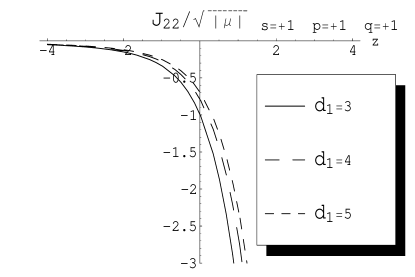
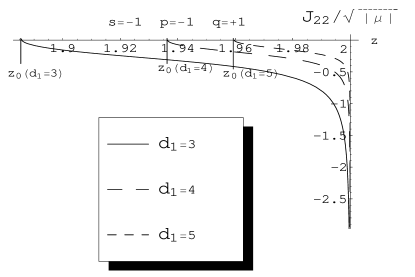
Figure 1: Typical form of $J_{22}/\sqrt{|\mu|}$ (eq. (4.9)) for parameters $s=+1,\;q=+1,\;p=+1$ (upper) and $s=-1,\;q=+1,\;p=-1$ (lower). For both of these combinations of the parameters, $J_{22}<0$.

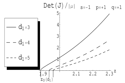
Figure 2: Typical form of $J_{22}/\sqrt{|\mu|}$ (upper) and $\mbox{det}(J)/|\mu|$ (lower) (see eqs. (4.8)-(4.10)) for parameters $s=-1,\;q=+1,\;p=+1$. For this combination of the parameters, $J_{22}>0$ and $\mbox{det}J>0$.

V Decoupling of excitations: $d_{1}=D_{0}$

It can be easily seen from eq. (II) that in the case $d_{1}=D_{0}$ parameter $c=0$ that leads to condition $\partial^{2}_{\varphi\phi}U_{eff}|_{extr}=0$ (see eq. (3.12). Thus the Hessian (3.4) is diagonalized. It means that the excitations of the fields $\varphi$ and $\phi$ near the extremum position are decoupled from each other.

Dropping the $h$ term in eq. (3.10) (because of $c=0$) and taking into account eq. (3.7), we obtain quadratic equation for $X$

$$(D+2)X^{2}+DqszX-(D-2)s=0\,,$$ (5.1)

which for $D_{0}=d_{1}$ exactly coincides with eq. (4.2). Thus, in spite of the fact that we does not use the condition $\Lambda_{eff}=0$, we obtain in the case $d_{1}=D_{0}$ precisely the same solutions (IV). However, parameters $R_{1},U_{0}$ and $h$ satisfy now relations different from (4.1). For example, for the most physically interesting case $D_{0}=d_{1}=4$, eqs. (3.9) and (3.8) result in the following relations:

$$R_{1}=4\left[\frac{1}{3}U_{0}(X)+h\right]\;,\quad\Lambda_{eff}(X)=\frac{1}{3}U_{0}(X)-h\,.$$ (5.2)

Nonzero components of the Hessian read

$$J_{11} = \frac{2}{3}\left[9h-U_{0}(X)\right]\>,\>$$ (5.3)

$$J_{22} = -\sqrt{|\mu|}\left[\frac{4(z+2qsX_{p})}{21(1+sX_{p}^{2})^{4/3}}+\frac{3qs(1+sX_{p}^{2})^{2/3}}{14X_{p}^{3}}\right].$$

In this section we are looking for a positive minimum of the effective potential. It means that $\Lambda_{eff}>0$, $J_{11}>0$ and $J_{22}>0$. From the positivity of $J_{11}$ and $\Lambda_{eff}$ we obtain respectively:

$$J_{11}>0:\quad 16h>R_{1}>16U_{0}(X)/9>8\Lambda_{eff}\;$$ (5.4)

and

$$\Lambda_{eff}>0:\quad h>R_{1}/16>U_{0}(X)/9>h/3>0\;.$$ (5.5)

These inequalities show that for the considered model positive minimum of the effective potential is possible only in the case of positive curvature of the internal space $R_{1}>0$ and in the presence of the form field $(h>0)$.

To realize which combination of parameters $s,p$ and $q$ ensures the minimum of the effective potential, we should perform analysis as in the previous case with $\Lambda_{eff}=0$. However, there is no need to perform such analysis here because solutions of eq. (5.1) coincides with (IV) and all conditions for $X_{p}$ and $U_{0}$ are the same as in the previous section. Thus, we obtain concluding table of the form (4.7). Additionally, it can be easily seen that expressions of $J_{22}$ in (5.3) and (4.9) exactly coincide with each other if we put $d_{1}=4$ in the latter equation. Hence, we can use Fig.1 and Fig.2 (for the lines with $d_{1}=4$) to analyze the sign of $J_{22}$. With the help of these pictures as well as keeping in the mind that $J_{22}(d_{1}=4,z=z_{0})=0$, we obtain that the only combination which ensures the positive minimum of $U_{eff}$ is: $s=-1\,,\;p=+1\,,\;q=+1\,$ and $z\in(z_{0}=1.936,+\infty)$. It is clear that potential $U_{0}(X)$ in eqs. (5.2)-(5.5) is defined by solution of eq. (5.1) (i.e. (IV) for $d_{1}=4$) with this combination of the parameters. Because $s=-1$ and $z>0$ , the parameters $\mu$ and $\Lambda_{D}$ should have the following signs: $\mu<0$ and $\Lambda_{D}>0$.

Additionally, it is easy to verify that second solution of eq. (5.1) $X_{-}$ (with $p=-1$ and $s=-1,\,q=+1$) does not correspond to the maximum of the effective potential $U_{eff}$. Indeed, we have here $\partial_{\phi}U_{eff}(X_{-})=0$ but $\partial_{\varphi}U_{eff}(X_{-})\neq 0$.

Fig. 3 demonstrates the typical profile $\varphi=0$ of the effective potential $U_{eff}(\varphi,\phi)$ in the case of positive minimum of $U_{eff}$ considered in the present section. This picture is in good concordance with the table (4.7). According to this table, positive extrema of $U_{eff}$ are possible only for the branch $q=+1$ of the solution (3.2) (solid lines in Fig. 3). We see that for $z_{0}<z<2$ we can have 3 such extrema: one for positive $\mu>0\to s=+1$ and two for negative $\mu<0\to s=-1$. Our investigations show that in the left half plane (i.e. for $\mu<0$) the right extremum ($p=+1$ in eq. (IV)) is the local minimum and the left maximum ($p=-1$) is not the extremum of $U_{eff}$ because here $\partial_{\varphi}U_{eff}\neq 0$. Analogously, maximum in the right half plane $\mu>0$ (which corresponds to ($p=+1$)-solution (IV)) is not the extremum of $U_{eff}$. For completeness of picture, we also included lines corresponding to the branch $q=-1$ (dashed lines in Fig. 3). The minimum of the right dashed line (for $X_{p}$ with $s=+1,\;p=-1,\;q=-1$) does not describe the extremum of $U_{eff}$ because again $\partial_{\varphi}U_{eff}\neq 0$.

Figure 3: Profile $\varphi=0$ of the effective potential $U_{eff}(\varphi,\phi)$ for parameters $z=1.99\;(\Lambda_{D}=1.99/2\;,\;|\mu|=1),\;D_{0}=d_{1}=4$ and $h=U_{0}/6$. The rest of parameters can be found from relations (5.2). Solid and dashed lines describe branches $q=+1$ and $q=-1$ respectively. For the solid line, there is only one local minimum of $U_{eff}$ which is defined by solution $X_{p}$ with the following parameters: $s=-1,\;p=+1,\;q=+1$. Left ($s=-1,\;p=-1,\;q=+1$) and right ($s=+1,\;p=+1,\;q=+1$) maxima are not extrema of $U_{eff}$ because in these points $\partial_{\phi}U_{eff}=0$ but $\partial_{\varphi}U_{eff}\neq 0$. Analogously, for right dashed line the solution $X_{p}$ (with $s=+1,\;p=-1,\;q=-1$) does not correspond to the extremum of $U_{eff}$.

VI cosmic acceleration and domain walls

Let us consider again the model with $d_{1}=D_{0}=4$ in order to define stages of the accelerating expansion of our Universe. It was proven that for certain conditions (see (5.2)-(5.5)) the effective potential $U_{eff}$ has local (for $z_{0}<z<2$) or global (for $z\geq 2$) positive minimum. The position of this minimum is $\left(\varphi=0,\,\phi=(1/A)\ln(1+sX^{2}_{p})\right)$ where $s=-1\,,\;p=+1\,,\;q=+1\,$ and $z\in(z_{0},+\infty)$. Obviously, positive minimum of the effective potential plays the role of the positive cosmological constant. Therefore, the Universe undergoes the accelerating expansion in this position. Thus, we can ”kill two birds with one stone”: to achieve the stable compactification of the internal space and to get the accelerating expansion of our external space.

We associate this acceleration with the late-time accelerating expansion of our Universe. As it follows from eqs. (5.2) and (5.5), positive minimum takes place if the parameters are positive and the same order of magnitude: $\Lambda_{eff}\sim R_{1}\sim U(X)\sim h>0$. On the other hand, in KK models the size of extra dimensions at present time should be $b_{(0)1}\lesssim 10^{-17}\mbox{cm}\sim 1\mbox{TeV}^{-1}$. In this case $R_{1}\gtrsim b_{(0)1}^{-2}\sim 10^{34}\mbox{cm}^{-2}$. Thus, for the TeV scale of $b_{(0)1}\sim 1$TeV we get that $\Lambda_{eff}\sim R_{1}\sim U(X)\sim h\sim 1\mbox{TeV}^{2}$. Moreover, in the case of natural condition $\Lambda_{D}\sim\sqrt{|\mu|}$ we obtain that the masses of excitations $m_{\varphi}\sim m_{\phi}\sim 1$TeV. The above estimates clearly demonstrate the typical problem of the stable compactification in multidimensional cosmological models because for the effective cosmological constant we obtain a value which is in many orders of magnitude greater than observable at the present time dark energy $\sim 10^{-57}\mbox{cm}^{-2}$. The necessary small value of the effective cosmological constant can be achieved only if the parameters $R_{1}\,,U(X)\,,h$ are extremely fine tuned with each other to provide the observed small value from equation $\Lambda_{eff}(X)=U_{0}(X)/3-h$. We see two possibilities to avoid this problem. Firstly, the inclusion of different form-fields/fluxes may result in a big number of minima (landscape) landscape1 -landscape4 with sufficient large probability to find oneself in a dark energy minimum. Secondly, we can avoid the restriction $R_{1}\sim b_{(0)1}^{-2}\sim 10^{34}\mbox{cm}^{-2}$ if the internal space is Ricci-flat: $R_{1}=0$. For example, the internal factor-space $M_{1}$ can be an orbifold with branes in fixed points (see corresponding discussion in Zhuk2006 ).

The WMAP three year data as well as CMB data are consistent with wide range of possible inflationary models (see e.g. WMAP2006 ). Therefore, it is of interest to get the stage of early inflation in our model. It is well known that it is rather difficult to construct inflationary models from multidimensional cosmological models and string theories. The main reason of it consists in the form of the effective potential which is a combination of exponential functions (see e.g. eq. (2.7)). Usually, degrees of these exponents are too large to result in sufficiently small slow-roll parameters (see e.g. GZBR ). Nevertheless, there is a possibility that in the vicinity of maximum or saddle points the effective potential is flat enough to produce the topological inflation topinfl ; SSTM ; R4 . Let us investigate this possibility for our model.

As stated above, the value $\varphi=0$ corresponds to the internal space value at the present time. Following this statement, we found the minimum of the effective potential at this value of $\varphi$. Obviously, the effective potential can also have extrema at $\varphi\neq 0$. Let us investigate this possibility for the model with $d_{1}=D_{0}=4$, i.e. for $c=0$. In this case, the extremum condition of the effective potential reads

$$\left.\partial_{\varphi}U_{eff}\right|_{\varphi_{0},\phi_{0}} = -\frac{1}{2}R_{1}(a+b)e^{(a+b)\varphi_{0}}+bU_{0}e^{b\varphi_{0}}$$ (6.1)

$$+ (ad_{1}+b)he^{(ad_{1}+b)\varphi_{0}}=0$$

and

$$\left.\partial_{\phi}U_{eff}\right|_{\varphi_{0},\phi_{0}}=\left.e^{b\varphi_{0}}\frac{\partial U}{\partial\phi}\right|_{\phi_{0}}=0\;;\;\Longrightarrow\;\left.\frac{\partial U}{\partial\phi}\right|_{\phi_{0}}=0\;.$$ (6.2)

Here, $\varphi_{0}$ and $\phi_{0}$ define the extremum position. It clearly follows from eq. (6.2) that $\phi_{0}$ is defined by equation $\partial U/\partial\phi=0$ which does not depend on $\varphi$. Therefore, extrema of the effective potential may take place only for $\phi_{0}$ which correspond to the solutions $X_{p}$ of eq. (5.1) and different possible extrema should lie on the sections $X_{p}=const$. So, we take $X_{+}$ (with $s=-1$ and $q=+1$) which defines the minimum of $U_{eff}$ in the previous section. Hence, $U_{0}$ in eq. (6.1) is the same as for eq. (5.2).

Let us define now $\varphi_{0}$ from eq. (6.1). With the help of inequalities (5.4) and (5.5) we can write $h=nU_{0}$ where $n\in(1/9,1/3)$. Taking also into account relations (5.2), eq. (6.1) can be written as

$$y^{4}-\left(1+\frac{1}{3n}\right)y+\frac{1}{3n}=0\,,$$ (6.3)

where we introduced the definition $y\equiv\exp{(a\varphi_{0})}=\exp{(\varphi_{0}/\sqrt{3})}$ and put $d_{1}=D_{0}=4$. Because $y=1$ is the solution of eq. (6.3), the remaining three solutions satisfy the following cubic equation:

$$y^{3}+y^{2}+y-\frac{1}{3n}=0\,.$$ (6.4)

It can be easily verified that the only real solution of this equation is

$$y_{0}=\frac{1}{3}\left(-1-2\nu+\frac{1}{\nu}\right)\;,$$ (6.5)

where

$$\nu = \frac{2^{1/3}n}{\left(9n^{2}+7n^{3}+3\sqrt{9n^{4}+14n^{6}+9n^{6}}\right)^{1/3}}\;;\;$$

$$n \in \left(\frac{1}{9},\frac{1}{3}\right)\;.$$ (6.6)

Thus $\varphi_{0}(y_{0})$ and $\phi_{0}(X_{+})$ define new extremum of $U_{eff}$. To clarify the type of this extremum we should check signs of the second derivatives of the effective potential in this point. First of all we should remember that in the case $c=0$ mixed second derivative disappears. Concerning second derivative with respect to $\phi$, we obtain

$$J_{22}\equiv\left.\frac{\partial^{2}U_{eff}}{\partial\phi^{2}}\right|_{\,\varphi_{0},\phi_{0}}=e^{b\varphi_{0}}\left.\frac{\partial^{2}U}{\partial\phi^{2}}\right|_{\,\phi_{0}}>0$$ (6.7)

because we got in previous section $\left.\partial^{2}U/\partial\phi^{2}\right|_{\,\phi_{0}(X_{+})}>0$. Second derivative with respect to $\varphi$ reads

$$J_{11} \equiv \left.\frac{\partial^{2}U_{eff}}{\partial\varphi^{2}}\right|_{\,\varphi_{0},\phi_{0}}=y_{0}^{2}U_{0}\left[-6\left(\frac{1}{3}+n\right)y_{0}+\frac{4}{3}\right.$$ (6.8)

$$+ \left.12ny_{0}^{4}\right]=2y_{0}^{2}U_{0}\left[(3n+1)y_{0}-\frac{4}{3}\right],$$

where we took into account eq. (6.3). Simple analysis shows that $(3n+1)y_{0}<4/3$ for $n\in(1/9,1/3)$. Keeping in mind that $U_{0}>0$ we obtain $J_{11}<0$. Therefore, our extremum is the saddle surface. Figure 4 demonstrates contour plot of the effective potential in the vicinity of the local minimum and the saddle point.

Figure 4: Contour plot of the effective potential $U_{eff}(\varphi,\phi)$ for parameters $z=1.99\;(\Lambda_{D}=1.99/2\;,\;|\mu|=1),\;D_{0}=d_{1}=4$ and $h=U_{0}/6$. The rest of parameters follows from relations (5.2). We choose the branch corresponding to $s=-1,\,q=+1$. This plot clearly shows the minimum and the saddle points of the effective potential.

Therefore, we arrived at very interesting possibility for the production of an inflating domain wall in the vicinity of the saddle point. The mechanism for the production of the domain walls is the following topinfl . If the scalar field $\varphi$ is randomly distributed, some part of the Universe will roll down to $\varphi=0$, while in others parts it will run away to infinity. Between any two such regions there will appear domain walls. In Ref. SSTM , it was shown for the case of a double-well potential $V_{dw}(\varphi)=(\lambda/4)(\varphi^{2}-\xi^{2})^{2}$ that a domain wall will undergo inflation if the distance $\xi$ between the minimum and the maximum of $V_{dw}$ exceeds a critical value $\xi_{cr}=0.33M_{Pl}\,\to\,\kappa_{0}\xi_{cr}=1.65$. In our case it means that the distance $|\varphi_{0}|$ between the local minimum and the saddle point should be greater than $\xi_{cr}$: $\,|\varphi_{0}|\geq 1.65$. Unfortunately, for our model $\varphi_{0}(n)<1.65$ if $n\in(1/9,1.3)$. For example, in the most interesting case $n\to 1/3$ (where $\Lambda_{eff}\to 0$ (see eq. (5.2))) we obtain $|\varphi_{0}|\to 1.055$ which is less than $\xi_{cr}$. Moreover, our domain wall is not thick enough in comparison with the Hubble radius. The ration of the characteristic thickness of the wall to the horizon scale is given by $r_{w}H\approx\left|U_{eff}/3\partial_{\varphi\varphi}U_{eff}\right|^{1/2}_{\varphi_{0},\phi(X_{+})}\to 0.454$ for $n\to 1/3$ which is less than the critical value 0.48 for a double-well potential. Thus, here there is no a sufficiently large (for inflation) quasi-homogeneous region of the energy density. Our potential is too steep. Obviously, the slaw roll parameter $\epsilon\approx(1/2)\left(\partial_{\varphi}U_{eff}/U_{eff}\right)^{2}_{\varphi_{0},\phi_{0}}$ is equal to zero in the saddle point. However, another slow roll parameter $\eta\approx\left|\partial^{2}_{\varphi\varphi}U_{eff}/U_{eff}\right|_{\varphi_{0},\phi_{0}}\to-1.617$ for $n\to 1/3$. Therefore, our domain walls do not inflate in contrast to the case $R^{4}$ in Ref. R4 .

In Fig. 5 we present comparison between our potential (solid line) and a double-well potential (dashed line) in the case $n=(1-0.001)/3$. We see that our potential is flatter than a double-well potential around the saddle point. However, our calculations show that it is not enough for inflation.

Figure 5: Comparison of the potential $U_{eff}(\varphi,\phi_{0})$ with a double well potential for parameters $z=1.99\;(\Lambda_{D}=1.99/2\;,\;|\mu|=1),\;D_{0}=d_{1}=4$ and $n=(1-0.001)/3$.

VII Conclusions and discussions

We have shown that positive minimum of the effective potential plays the double role in our model. Firstly, it provides the freezing stabilization of the internal spaces which enables to avoid the problem of the fundamental constant variation in multidimensional models (Zhuk(IJMP) -BZ ). Secondly, it ensures the stage of the cosmic acceleration. However, to get the present-day accelerating expansion, the parameters of the model should be fine tuned. Maybe, this problem can be resolved with the help of the idea of landscape of vacua (landscape1 -landscape4 ). We intend to investigate this possibility in our forthcoming paper.

We have additionally found that our effective potential has the saddle point. It results in domain walls which separates regions with different vacua in the Universe. These domain walls do not undergo inflation because the effective potential is not flat enough around the saddle point.

It is worth of noting that minimum in Fig. 3 (left solid line) is metastable. In other words, classically it is stable but there is a possibility for quantum tunnelling both in $\phi$ and in $\varphi$ directions (see Fig. 4). We can avoid this problem in $\phi$ direction in the case of parameters $z\geq 2$ (see footnote 7). However, tunnelling in $\varphi$ direction (through the saddle) is still valid because $U_{eff}(\varphi,\phi_{0})\approx e^{b\varphi}U(\phi_{0})\rightarrow 0$ for $\varphi\rightarrow-\infty$ which is less than any positive $\Lambda_{eff}$. It may result in the materialization of bubbles of the new phase in the metastable one (see e.g. Rubakov ). Thus, late-time acceleration is possible only if characteristic lifetime of the metastable stage is greater than the age of the Universe. Careful investigation of this problem (including gravitational effects) is rather laborious task which needs a separate consideration. As we mentioned in footnote 8, there is also the global negative minimum for right dashed line in Fig. 3 (it corresponds to the point $(\varphi=0.67,\phi=1.66)$ for parameters taken in Fig. 3). This minimum is stable both in classical and quantum limits. However, the acceleration is absent because of its negativity.

Another very interesting feature of the model under consideration consists in multi-valued form of the effective potential. As it can be easily seen from eqs. (2.7) and (3.3), for each choice of parameter $\mu$ potential $U(\phi)$ (and consequently $U_{eff}$) has two branches ($q=\pm 1$) which joint smoothly with each other at $\phi=0$ (see Fig. 3). It gives very interesting possibility to investigate transitions from one branch to another one by analogy with catastrophe theory or similar to the phase transitions in statistical theory. However, as we mentioned above, in our particular model the point $\phi=0$ corresponds to the singularity $\bar{R},R\to\pm\infty$. Thus, the analog of the second order smooth phase transition through the point $\phi=0$ is impossible in our model. Nevertheless, there is still a possibility for the analog of the first order transition via quantum jumps from one branch to another one. In what follows, we plan to investigate such ”phase transitions” for non-linear multidimensional models $f(R)$.

To complete the paper, we investigate some limiting cases. Firstly, we consider the limit $h\to 0$ (for arbitrary $D_{0}$ and $d_{1}$) where the form-fields are absent. From eqs. (3.7) - (3.13) we obtain the following system of equations:

$$R_{1}=\frac{2b}{a+b}U_{0}(X)\,,\quad\left.U_{eff}\right|_{extr}=\frac{a}{a+b}U_{0}(X)$$ (7.1)

and

$$J_{11} = -ab\,U_{0}(X)\,,\quad J_{21}=0\,,\;$$

$$J_{22} = \left[B(A-B)-\frac{sAB}{2X^{2}}(1+sX^{2})\right]U_{0}(X)\,.\qquad$$ (7.2)

Since for minimum should hold true the condition $J_{11}>0$, we arrive at the conclusion: $R_{1},\,U_{0},\,U_{eff}<0$. Consequently, the minimum of the effective potential as well as the effective cosmological constant is negative and accelerating expansion is absent in this limit. Therefore, the presence of the form-fields is the necessary condition for the acceleration of the Universe in the position of the freezing stabilization of the internal spaces. Additionally, it can be easily seen that the extremum position equation takes the same form as (5.1). Simple analysis show that minimum takes place for the branch: $s=+1$ (i.e. $\mu>0$), $p=-1,\,q=-1$ and $z\in(-\infty,+\infty)$. If additionally we demand $z\to 0$ (i.e. $\Lambda_{D}\to 0$ and $\mu$ is fixed) then we reproduce the results of Ref. GZBR .

Acknowledgments

We are grateful to Alex Vilenkin for his very useful comments concerning the fine tuning problem and its possible resolution with the help of the idea of landscape.

References

- (1) D. N. Spergel et al, Wilkinson Microwave Anisotropy Probe (WMAP) Three Year Results: Implications for Cosmology, astro-ph/0603449.
- (2) S. Capozziello, S. Carloni and A. Troisi, Quintessence without scalar field,”Recent Research Developments in Astronomy and Astrophysics”-RSP/AA/21-2003, astro-ph/0303041; S.M. Carroll, V. Duvvuri, M. Trodden and M.S. Turner, Phys.Rev. D70, (2004), 043528, astro-ph/0306438; D.N. Vollick, Phys. Rev. D68, (2003), 063510, astro-ph/0306630; R. Dick, Gen. Rel. Grav. 36, (2004), 217, gr-qc/0307052; A.D. Dolgov and M. Kawasaki, Phys. Lett. B573, (2003), 1, astro-ph/0307285; S. Nojiri and S.D. Odintsov, Phys. Rev. D68, (2003), 123512, hep-th/0307288; S. Nojiri and S.D. Odintsov, Mod.Phys.Lett. A19 (2004) 627, hep-th/0307288; T. Chiba, Phys. Lett. B575, (2003), 1, astro-ph/0310045; X. Meng and P. Wang, Class. Quant. Grav. 20, (2003), 4949, astro-ph/0307354; G. M. Kremer and D. S. M. Alves, Phys.Rev. D70, (2004), 023503, gr-qc/0404082; N. Furey and A. DeBenedictis, Class.Quant.Grav. 22, (2005), 313, gr-qc/0410088; F. P. Schuller and M. N.R. Wohlfarth, Phys.Lett. B612, (2005), 93, gr-qc/0411076; S. Nojiri and S.D. Odintsov, Introduction to modified gravity and gravitational alternative for dark energy, hep-th/0601213; L.Amendola, D.Polarski and S.Tsujikawa, Are dark energy models cosmologically viable?, astro-ph/0603703; E.J. Copeland, M.Sami, S.Tsujikawa, Int.J.Mod.Phys. D15, (2006), 1753, hep-th/0603057; Anthony W. Brookfield, Carsten van de Bruck, Lisa M.H. Hall, Phys.Rev. D74, (2006), 064028, hep-th/0608015; T.P. Sotiriou, Phys.Lett. B645, (2007), 389, gr-qc/0611107.
- (3) S. Nojiri and S.D. Odintsov, Phys. Lett. B576, (2003), 5, hep-th/0307071;
- (4) S. M. Carroll, A. De Felice, V. Duvvuri, D. A. Easson, Mark Trodden and M. S. Turner, Phys.Rev. D71, (2005), 063513, astro-ph/0410031.
- (5) A. Zhuk, Int. Journ. Mod. Phys. D11, (2002), 1399, hep-ph/0204195.
- (6) P. Loren-Aguilar, E. Garcia-Berro, J. Isern, and Yu.A. Kubyshin, Class. Quant. Grav. 20, (2003), 3885, astro-ph/0309723 .
- (7) U. Günther, A. Starobinsky and A. Zhuk, Phys. Rev. D 69, (2004), 044003, hep-ph/0306191.
- (8) V. Baukh and A. Zhuk, Phys. Rev. D73, (2006), 104016, hep-th/0601205.
- (9) J.-M. Alimi, V.D. Ivashchuk, S.A. Kononogov and V.N. Melnikov, Gravitation & Cosmology, 12, (2006), 173, gr-qc/0611015.
- (10) J.-P. Uzan, Rev. Mod. Phys. 75, (2003), 403, hep-ph/0205340.
- (11) U. Günther and A. Zhuk, Phys. Rev. D 56, (1997), 6391, gr-qc/9706050.
- (12) U. Günther, A. Zhuk, V.B. Bezerra and C. Romero, Class. Quant. Grav. 22, (2005), 3135, hep-th/0409112.
- (13) U. Günther, P. Moniz and A. Zhuk, Phys. Rev. D 68, (2003), 044010, hep-th/0303023.
- (14) U. Günther, P. Moniz and A. Zhuk, Phys. Rev. D 66, (2002), 044014, hep-th/0205148.
- (15) U. Günther, P. Moniz and A. Zhuk, Astrophysics and Space Science 283, (2003), 679, gr-qc/0209045.
- (16) P.G.O. Freund and M.A. Rubin, Phys. Lett. B 97, (1980), 233.
- (17) U. Günther and A. Zhuk, Phys. Rev. D 61, (2000), 124001, hep-ph/0002009.
- (18) M. Rainer and A. Zhuk, Phys. Rev. D 54, (1996), 6186, gr-qc/9608020.
- (19) V.D.Ivashchuk and V.N.Melnikov, Class.Quant.Grav. 12, (1995) 809, gr-qc/9407028; A.Zhuk, Class.Quant.Grav. 13, (1996) 2163; U.Gunther and A.Zhuk, Class.Quant.Grav. 15, (1998) 2025, gr-qc/9804018.
- (20) R. Bousso and J. Polchinski, JHEP 0006, (2000), 006, hep-th/0004134.
- (21) L. Susskind, The anthropic landscape of string theory; hep-th/0302219.
- (22) R. Kallosh and A. Linde, JHEP 0412, (2004), 004, hep-th/0411011.
- (23) D. Schwartz-Perlov and A. Vilenkin, JCAP 0606, (2006), 010, hep-th/0601162.
- (24) A. Zhuk, Conventional cosmology from multidimensional models; hep-th/0609126.
- (25) A. Linde, Phys. Lett. B 327, (1994) 208, hep-th/9402031; A. Vilenkin, Phys. Rev. Lett. 72, (1994), 3137, hep-th/9402085.
- (26) N. Sakai, H. Shinkai, T. Tachizawa and K. Maeda, Phys.Rev. D 53, (1996) 655; Erratum-ibid. D 54, (1996) 2981, gr-qc/9506068.
- (27) J. Ellis, N. Kaloper, K. A. Olive and J. Yokoyama, Phys.Rev. D 59, (1999) 103503, hep-ph/9807482.
- (28) V.A. Rubakov and S.M. Sibiryakov, Theor.Math.Phys., 120 (1999), 1194, gr-qc/9905093.