Mass Spectrum of Dirac Equation with
Local Parabolic Potential

Abstract

In this paper, we solve the eigen solutions and mass strectra of the Dirac equation with local parabolic potential which is approximately equal to the short distance potential generated by spinor itself. The mass spectrum is quite different from that of a spinor in Coulomb potential. The masses of some baryons are similar to this one. The mass-angular momentum relation $m=m(J,n)$ is quite similar to the Regge trajectories. The parabolic potential has property of asymptotic freedom near the center and confinement at large distance. So the results imply that, the local parabolic potential may be more suitable for describing nuclear potential approximately. The solving procedure can also be used to solve the Dirac equation with other complicated potential.

Keywords: Regge trajectory, parabolic potential, mass spectrum, baryon, short distance potential

I Introduction

For hadrons, the relation between mass $m$ and quantum numbers $(J,n)$ is usually described by the Regge-Chew-Frautschi formula1 ; 2 ,

$$m^{2}=an+bJ+m_{0},$$ (1.1)

where $(a,b,m_{0})$ are constants for the exited states of the same kind particle. In many cases, the factors satisfies $b\leq a\leq 2b$3 ; 4 . The Regge trajectory is an important tool widely used to analyze the spectroscopy of mesons and baryons. Various theoretical models have been constructed to explain the mass spectra of particles and to derive the Regge trajectories, such as non-relativistic quark models 5 ; 6 ; 7 ; 8 ; 9 ; 10 ; 25 ; [260] ; 11 , flux tube model or similar string model3 ; 12 ; 13 ; 14 ; 15 ; 16 ; 17 ; 18 ; 19 ; 20 , semi-relativistic model 21 ; 22 ; 23 ; 24 , relativistic model 26 ; 27 ; 28 ; 29 ; 30 , quantum chromodynamics (QCD) sum rule 31 ; 32 ; 33 , color hyperfine interaction 34 ; 35 ; 36 ; 37 , Lattice QCD modellatt ; 38 ; 39 ; 40 ; 41 and so on. There are also some Regge phenomenology investigations3 ; 42 ; 43 ; 44 ; 45 ; 46 ; 47 . By statistical and regressive method to get the relation $m=f(J,n)$.

In many models, the total potential between quarks is given by Cornell potential with some hyperfine terms of correction, and the mass spectrum is solved in relative Jacobi coordinates8 ; 10 ; 11 ; 29 ; 30 ; 34 ; 48 . In 48 , by semi classical approximation and Bohr-Sommerfeld quantization, the Regge-like relation $E\sim L^{2\alpha/(\alpha+2)}$ and $E\sim n^{2\alpha/(\alpha+2)}$ for large $(n,L)$ is derived for power-law confining potentials $V\propto r^{\alpha}$. By the phenomenological researches, we also find that the Regge-Chew-Frautschi formula (1.1) is only approximately valid, and a little nonlinearity always exists42 ; 43 ; 45 . The specific Regge trajectories depend on concrete confining potential. However, no matter what confining potential is, the analytic relation $m=f(J,n)$ for the excited states always exists.

Recently, a number of experimental data for highly exited resonances were reported 49 ; 50 ; 51 ; 52 ; 53 ; 54 ; 55 ; 56 ; 57 . These data provide opportunity to check the previous calculations and develop more effective models. As pointed out in 57 , A better understanding of the nucleon as a bound state of quarks and gluons as well as the spectrum and internal structure of excited baryons remains a fundamental challenge and goal in hadronic physics. In particular, the mapping of the nucleon excitations provides access to strong interactions in the domain of quark confinement. While the peculiar phenomenon of confinement is experimentally well established and believed to be true, it remains analytically unproven and the connection to quantum chromodynamics (QCD) - the fundamental theory of the strong interactions - is only poorly understood. In the early years of the 20th century, the study of the hydrogen spectrum has established without question that the understanding of the structure of a bound state and of its excitation spectrum need to be addressed simultaneously. The spectroscopy of excited baryon resonances and the study of their properties is thus complementary to understanding the structure of the nucleon in deep inelastic scattering experiments that provide access to the properties of its constituents in the ground state.

The quark models employ multiplets of spinors and nonlinear interactive vectors with gauge symmetries, which are too complicated to get exact solutions and an overview for the properties. In this paper we examine the following simple and closed Dirac equation with short range self-generating vector potential $\Phi_{\mu}$,

$${\cal L}=\phi^{+}\alpha^{\mu}(i\partial_{\mu}-s\Phi_{\mu})\phi-\mu c\check{\gamma}+\frac{1}{2}(\partial_{\mu}\Phi_{\alpha}\partial^{\mu}\Phi^{\alpha}-b^{2}\Phi_{\mu}\Phi^{\mu}),$$ (1.2)

in which $\check{\gamma}=\phi^{+}\gamma\phi$. (1.2) has plentiful spectra. By the Regge trajectories we find the excited states may be relevant to some of baryons.

II Equations and Simplification

At first, we introduce some notations. Denote the Minkowski metric by $\eta_{\mu\nu}={\rm diag}(1,-1,-1,-1)$, Pauli matrices by

$${\vec{\sigma}}=(\sigma^{j})=\left\{\left(\begin{array}[]{cc}0&1\\ 1&0\end{array}\right),\left(\begin{array}[]{cc}0&-i\\ i&0\end{array}\right),\left(\begin{array}[]{cc}1&0\\ 0&-1\end{array}\right)\frac{}{}\right\}.$$ (2.7)

Define $4\times 4$ Hermitian matrices as follows

$$\alpha^{\mu}=\left\{\left(\begin{array}[]{cc}I&0\\ 0&I\end{array}\right),\left(\begin{array}[]{ll}0&\vec{\sigma}\\ \vec{\sigma}&0\end{array}\right)\right\},\quad\gamma=\left(\begin{array}[]{cc}I&0\\ 0&-I\end{array}\right),\quad\beta=\left(\begin{array}[]{cc}0&-iI\\ iI&0\end{array}\right)$$ (2.16)

where $\mu\in\{0,1,2,3\}$, $x^{0}=ct$ and $\alpha^{\mu}=\gamma^{0}\gamma^{\mu}$. By variation of (1.2) we get the Dirac equation and dynamics of $\Phi^{\mu}$,

$$\alpha^{\mu}(\hbar i\partial_{\mu}-s\Phi_{\mu})\phi = \mu c\gamma\phi.$$ (2.17)

$$\partial_{\alpha}\partial^{\alpha}\Phi^{\mu}+b^{2}\Phi^{\mu} = -s\check{\alpha}^{\mu},\quad\check{\alpha}^{\mu}=\phi^{+}\alpha^{\mu}\phi.$$ (2.18)

For the eigen states of $\phi$, only the magnetic quantum number $m_{z}$ and the sipn $s$ are conserved. So the eigen solution takes the following form

$$\phi=(u_{1},u_{2}e^{\varphi i},-iv_{1},-iv_{2}e^{\varphi i})^{T}\exp(m_{z}\varphi i-\frac{mc^{2}}{\hbar}it),$$ (2.19)

where the index $T$ stands for transpose, $m_{z}\in\{0,\pm 1,\pm 2,\cdots\}$, and $u_{k},v_{k}(k=1,2)$ are real functions of $r$ and $\theta$. However, the exact solution of (2.19) does not exist, and we have to solve it by effective algorithmgu1 ; 58 . Since the numerical solutions are also unhelpful to understand the global structure of the mass spectrum, we seek for the approximate analytic solutions in this paper.

Different from the case of an electron, a proton has a hard core with charge distribution, and the radius of the distribution is about $1\times 10^{-15}m$. The following calculation shows the local parabolic potential is approximately equal to $\Phi_{\mu}$ near the center, then we have

$$\Phi_{0}\dot{=}\left(\frac{w^{2}r^{2}}{2\rho^{2}}-{2(1-\eta)}\right)\mu c,\quad\vec{\Phi}\dot{=}0,\quad(r<12\rho),$$ (2.20)

in which $w$ is the strength factor, $\eta$ is a parameter to adjust the depth of confinement to fit the true confining potential. $\rho=\frac{\hbar}{\mu c}$ is the theoretical Compton wave length, which is used for nondimensionalization of the Dirac equation.

In order to simplify (1.2), we make transformation58

$$g=u_{1}+u_{2}i\qquad f=v_{1}-v_{2}i.$$ (2.21)

Substituting (2.19), (2.20) and (2.21) into (1.2) we get Lagrangian as

$${\cal L}=({\cal L}_{0}+{\cal L}_{f})\mu c,$$ (2.22)

in which we defined

$${\cal L}_{0} \equiv \Re\langle e^{\theta i}\left(-\bar{g}(\partial_{r}+\frac{i}{r}\partial_{\theta})f+f(\partial_{r}+\frac{i}{r}\partial_{\theta})\bar{g}\right)\rangle\rho-\frac{i}{r\sin\theta}(m_{z}+\frac{1}{2})(\bar{g}\bar{f}-gf)\rho$$ (2.23)

$$+\varepsilon(|g|^{2}+|f|^{2})+\left(\frac{w^{2}r^{2}}{2\rho^{2}}-2(1-\eta)\right)|g|^{2}-(2+\kappa)|f|^{2},$$

where $\Re\langle\rangle$ stands for taking real part, and

$${\cal L}_{f}\equiv\left(\kappa+\frac{w^{2}r^{2}}{2\rho^{2}}-{2(1-\eta)}\right)|f|^{2}.$$ (2.24)

In (2.23) $\varepsilon$ is relative mass defect defined by

$$mc^{2}=(1-\varepsilon)\mu c^{2},\qquad\varepsilon=\frac{\mu-m}{\mu},$$ (2.25)

and $\rho$ is used as length unit, $\kappa$ is a constant to let $|\int_{0}^{\infty}{\cal L}_{f}r^{2}dr|\to 0$ so that convergent rate of the procedure is optimized. In the case (2.20) we set $\kappa=(1-\eta)$ which is about the mean value of the potential in the effective domain, and then ${\cal L}_{f}$ can be omitted for the $0th$ order approximation. For proton we have

$$\rho=\frac{\hbar}{\mu c}=(1-\varepsilon)\frac{\hbar}{m_{p}c},\leavevmode\nobreak\ \leavevmode\nobreak\ \lambda=\frac{\hbar}{m_{p}c}=2.1037\times 10^{-16}{\rm m}.$$ (2.26)

In (2.22), ${\cal L}_{0}$ almost keeps all invariance of relativity and has simple and complete eigensolutions, which can be used as the bases of Hilbert space of representation. ${\cal L}_{f}$ is the trouble terms with small energy, which acts as perturbation in the calculation. If taking $\mu c=1,\rho=1$, (2.22) becomes dimensionless.

For (2.23), the rigorous eigensolutions take the following form58

$$g=U(r)[P(\theta)+Q(\theta)i],\qquad f=V(r)[P(\theta)+Q(\theta)i]e^{-i\theta}.$$ (2.27)

By variation of (2.23) we get

$$\partial_{\theta}P = \cot\theta m_{z}P+(m_{z}+K)Q,$$ (2.28)

$$\partial_{\theta}Q = -\cot\theta(m_{z}+1)Q+(m_{z}+1-K)P,$$ (2.29)

in which $K=\pm 1,\pm 2,\cdots$ corresponding to orbital angular momentum, $P,Q$ are associated Legendre functions. The radial functions satisfy

$$\partial^{2}_{r}U+\frac{2}{r}\partial_{r}U-\left(\frac{K(K-1)}{r^{2}}-\frac{2{\cal E}}{\rho^{2}}+\frac{\left(3-\varepsilon-\eta\right)w^{2}r^{2}}{2\rho^{4}}\right)U=0,$$ (2.30)

$$V=\frac{\left(r\partial_{r}U-(K-1)U\right)\rho}{(3-\varepsilon-\eta)r},$$ (2.31)

in which we defined

$${\cal E} = \frac{1}{2}(2-\varepsilon-2\eta)(3-\varepsilon-\eta)$$ (2.32)

$$= \frac{1}{2}\left((1-2\eta)(2-\eta)+3(1-\eta)M+M^{2}\right),$$ (2.33)

$${\rm Or\leavevmode\nobreak\ inversely,}\leavevmode\nobreak\ \leavevmode\nobreak\ \leavevmode\nobreak\ \varepsilon = \frac{1}{2}\left(5-3\eta-\sqrt{(1+\eta)^{2}+8{\cal E}}\right),$$ (2.34)

where $M=\frac{m}{\mu}$ is dimensionless mass. The above equations can be easily solved, and the solutions are all elementary functions. The normalizing conditions are as follows

$$\int_{0}^{\pi}(P^{2}+Q^{2})2\pi\sin\theta d\theta=1,\quad\int_{0}^{\infty}(U^{2}+V^{2})r^{2}dr=1.$$ (2.35)

III Eigen Solutions to the equation

For (2.30), we have the solution

$$U = \left(C_{1}r^{K-1}+C_{2}r^{-K}\right)L_{n-1}^{J}\left(\frac{2r^{2}}{r_{n}^{2}}\right)\exp\left(-\frac{r^{2}}{r_{n}^{2}}\right),$$ (3.1)

$$n = 1,2,3,\cdots,\qquad J=\left|K-\frac{1}{2}\right|=\frac{1}{2},\frac{3}{2},\frac{5}{2},\cdots,$$ (3.2)

where $L_{n-1}^{J}$ is associated Laguerre polynomials, $n$ is radial quantum number, and $J$ is angular momentum quantum number. $C_{1}=0$ corresponding to $K<0$ and $C_{2}=0$ corresponding to $K>0$. The energy spectrum and radius parameter is given by

$$Nw = \frac{{\cal E}}{\sqrt{1+\eta+\sqrt{(1+\eta)^{2}+8{\cal E}}}},\qquad N=n+\frac{1}{2}({J-1}),$$ (3.3)

$$r_{n} = 2\rho\sqrt{\frac{N}{{\cal E}}}={2M\lambda}\sqrt{\frac{N}{{\cal E}}}.$$ (3.4)

Substituting (2.33) into (3.3) we get Regge-like relation as follows

$$2n+J-1=\frac{\sqrt{2}}{2w}\left(1-2\eta+M\right)\sqrt{2-\eta+M}.$$ (3.5)

Or inversely,

$$M = \frac{1}{36}{{\cal{N}}}^{\frac{2}{3}}+4{{\left(1+\eta\right)^{2}}{{{\cal{N}}}^{-\frac{2}{3}}}}+\frac{1}{3}(5\eta-4),$$ (3.6)

$${\cal{N}} = 216\,Nw\sqrt{2}+24\,\sqrt{162\,{N}^{2}{w}^{2}-3\,\left(1+\eta\right)^{3}}.$$ (3.7)

In (3.5) we have 3 constants $(w,\eta,\mu)$ for the same series of particles to be determined by empirical data. Although the form of (3.5) or (3.6) is quite different from (1.1), the following calculation shows that the curves of (3.5) in the effective domain is quite near straight lines(see Fig.1).

Substituting (3.1) and (3.3) into (2.31), we can derive $V$. By calculation we get

$$\int_{0}^{\infty}U^{2}_{K,n}r^{2}dr=\frac{(1+\eta)\sqrt{(1+\eta)^{2}+8{\cal E}}+(1+\eta)^{2}+4{\cal E}}{(1+\eta)\sqrt{(1+\eta)^{2}+8{\cal E}}+(1+\eta)^{2}+6{\cal E}}.$$ (3.8)

For all meaningful eigensolutions we have $0.1<{\cal{E}}<4$, and then we have $\int_{0}^{\infty}U^{2}_{K,n}r^{2}dr=0.8\sim 1$. Therefore, the relative truncation error for the $0th$ approximation is about $10\%$.

The ground state corresponds to $n=1,J=\frac{1}{2}$, and then we have $N=\frac{3}{4}$. Considering energy degeneracy, we only need to calculate the energy spectrums while $K\geq 1$. For the ground state of proton, we have empirical data $r_{n}\sim 1\times 10^{-15}{\rm m}$ and $m_{p}=938.28$MeV. Substituting them and $N=\frac{3}{4}$ into (2.25), (2.26),(2.32) and (3.4), we get constants $(w,\eta,\rho,\mu,\varepsilon_{0})$ expressed by ${\cal E}_{0}$. If taking ${\cal E}_{0}=0.17618$, we have solution

$$\eta=0.74238,\leavevmode\nobreak\ w=0.11972,\leavevmode\nobreak\ \varepsilon_{0}=0.33220,\leavevmode\nobreak\ \rho=1.4048\times 10^{-16}{\rm m},\leavevmode\nobreak\ \mu c^{2}=1.4051{\rm GeV}.$$ (3.9)

For a proton, by (3.9) we find $r_{n}\sim 7\rho$. By (2.25) and $\varepsilon_{0}$ we find the relative mass defect of strong interaction confinement is about $33\%$. The observational mass $m_{p}$ is much less than constant mass $\mu$. This case is quite different from an electron without strong interaction.

Substituting (3.9) and $(J,n)$ into (3.5), (3.6) and (3.7), we get the mass spectra of the particles $m(J,n)$ shown in Tab.1. We find the masses of many baryons are near the spectra, and (3.5) is quite similar to the Regge trajectories of baryons(see Fig.1). By (3.3) and (3.4), we find the radius parameter $r_{n}$ of the excited states even decreases a little when the quantum number $N$ increases. Detailed calculation shows we always have $\bar{r}=(4\sim 10)\rho$ for all particles. This means a particle with local parabolic potential or short distance potential $\Phi_{\alpha}$ has a very hard core. This phenomenon is quite different from the case of Coulomb potential, where we have $\bar{r}\propto n^{2}$.

Table 1: Mass spectra of Dirac equation with local parabolic potential(MeV)

$m(J,n)$	1	2	3	4	5	6	7	8	9	10	11	12	13	14
1/2	938	1249	1535	1801	2052	2291	2520	2740	2953	3159	3359	3554	3744	3930
1+1/2	1098	1395	1670	1928	2173	2407	2631	2847	3056	3260	3457	3650	3838	4022
2+1/2	1249	1535	1801	2052	2291	2520	2740	2953	3159	3359	3554	3744	3930	4112
3+1/2	1395	1670	1928	2173	2407	2631	2847	3056	3260	3457	3650	3838	4022	4202
4+1/2	1535	1801	2052	2291	2520	2740	2953	3159	3359	3554	3744	3930	4112	4290
5+1/2	1670	1928	2173	2407	2631	2847	3056	3260	3457	3650	3838	4022	4202	4378
6+1/2	1801	2052	2291	2520	2740	2953	3159	3359	3554	3744	3930	4112	4290	4465
7+1/2	1928	2173	2407	2631	2847	3056	3260	3457	3650	3838	4022	4202	4378	4552
8+1/2	2052	2291	2520	2740	2953	3159	3359	3554	3744	3930	4112	4290	4465	4637
9+1/2	2173	2407	2631	2847	3056	3260	3457	3650	3838	4022	4202	4378	4552	4722
10+1/2	2291	2520	2740	2953	3159	3359	3554	3744	3930	4112	4290	4465	4637	4806
11+1/2	2407	2631	2847	3056	3260	3457	3650	3838	4022	4202	4378	4552	4722	4889
12+1/2	2520	2740	2953	3159	3359	3554	3744	3930	4112	4290	4465	4637	4806	4972
13+1/2	2631	2847	3056	3260	3457	3650	3838	4022	4202	4378	4552	4722	4889	5054
14+1/2	2740	2953	3159	3359	3554	3744	3930	4112	4290	4465	4637	4806	4972	5135
15+1/2	2847	3056	3260	3457	3650	3838	4022	4202	4378	4552	4722	4889	5054	5216

We find the masses of many baryons are near the spectra. Obviously each excited state should correspond to an observable particle. This means some baryons can be regarded as excited resonances of a proton. How to exactly identify the quantum numbers for each particle observed in experiments is an important but fallible problem.

As the $0th$ order approximation with only 3 free coefficients, the result is satisfactory. To get more accurate solutions of (1.2), we can expand $\phi$ as series of the eigen functions of (2.23) and then solve mass spectra of (1.2)58 . However, in this case we have only numerical results without an overview on the spectra.

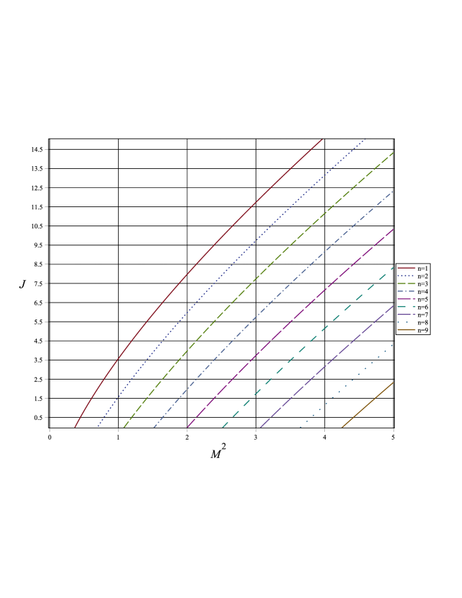
Figure 1: Regge trajectroies of (3.5). Each intersection between lines $J=\frac{1}{2}+j$ and curves $J=J(n,M^{2})$ corresponds to one or more particles, and we have about 90 intersections in the figure. Considering degenerate states, the figure contains more than 1000 particles with different quantum numbers $(n,K,m_{z},s)$.

IV Effectiveness of the Parabolic Potential

Now we check the effectiveness of the parabolic potential for nuclear potential. It is well known the global parabolic potential cannot be used as confining potential of Dirac equation. However, the following calculations show the local parabolic potential is effective to describe nuclear potential approximately.

At first, we check all radial functions $(U_{K,n},V_{K,n})$ and their module $U^{2}+V^{2}$ are almost distributed in the domain $r<12$, where is also the effective area of the local parabolic potential. The first couple of the radial functions is given by

$$U_{1,1}=0.29450687e^{-0.05873333r^{2}},\quad V_{1,1}=-0.01796750re^{-0.05873333r^{2}},$$ (4.1)

we find $|V/U|^{2}\sim 1\%$. See Fig.2 and Fig.3 as follows, where we take $\rho=1$ as length unit.

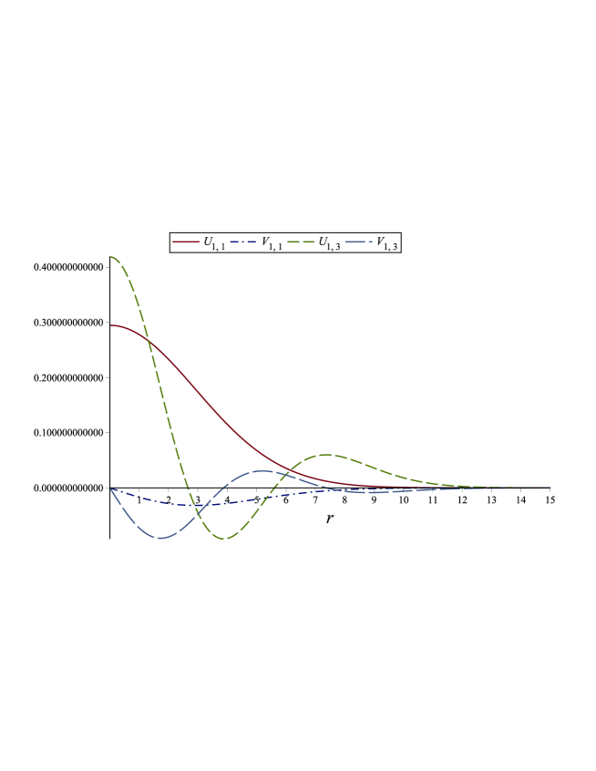
Figure 2: Some radial wave functions of a spinor in local parabolic potential.

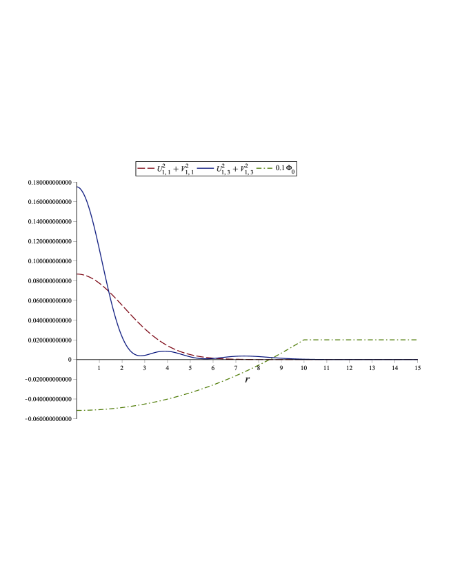
Figure 3: The effective domain of local parabolic potential and modules of radial wave functions. The spinor with short distance potential is mainly concentrated near the center, and it does not diffuse when $K$ or $n$ increases.

Secondly, for the following short range potential $\Phi$ with source $q(r)$,

$$\partial_{\alpha}\partial^{\alpha}\Phi+\frac{1}{\rho^{2}}\Phi=-65\cdot\frac{4\pi q(r)}{\rho^{3}}.$$ (4.2)

By Fig.4, we find the solution $\Phi$ is almost parabolic potential $\Phi_{0}$ in the domain $r<8$ for the above source, for which the normalizing condition is $4\pi\int q(r)r^{2}dr=1$. This means in the interior of a baryon, the potential of strong interaction may be different from the Cornell potential or potential generated by point source $-\frac{e^{-r}}{r}$ or the MIT bag model. It may be more suitably described by local parabolic potential.

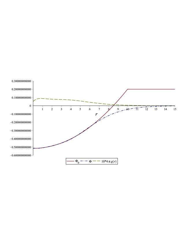
Figure 4: The parabolic potential versus the short range potential generated by $q(r)$.

Thirdly, by (3.3) we find that, different from electron in Coulomb potential, in this case the radius parameter $r_{n}$ of the wave function even decreases a little as the increasing of quantum number $N$. So the local parabolic potential is also suitable for the excited states.

V Discussion and Conclusion

As the $0th$ order approximation, the above calculation provides some important messages. The Dirac equation with short distance potential has quite different energy spectrum and eigen functions from that with Coulomb potential. Dirac equation is a magic equation with marvellous properties which should be strictly analyzedeng ; gu2 ; engc . The nuclear potential may be more similar to local parabolic potential, rather than the MIT bag model or $-\frac{e^{-r}}{r}$ or $-\frac{\alpha_{s}}{r}-ar$. Obviously, the spinor in short distance potential (4.2) has the asymptotic freedom near the center and strong confinement near $r\sim 10\rho$(see Fig.3 and Fig.4).

To get more accurate results, we should directly solve the coupling system of (2.18) and (2.17), and expand the radial functions $(U,V)$ upon the bases $U_{K,n},V_{K,n}$ of the representation space58 . However, in this case we have not explicit analytic expression (3.3) for mass spectra.

As the alternative models for fundamental particles, some simple and closed systems such as the following one are worth to be carefully studied,

$${\cal L} = \phi^{+}\alpha^{\mu}(i\partial_{\mu}-eA_{\mu}-s\Phi_{\mu})\phi-\mu c\check{\gamma}+F(\check{\gamma},\check{\beta})$$ (5.1)

$$-\frac{1}{2}\partial_{\mu}A_{\alpha}\partial^{\mu}A^{\alpha}+\frac{1}{2}(\partial_{\mu}\Phi_{\alpha}\partial^{\mu}\Phi^{\alpha}-b^{2}\Phi_{\mu}\Phi^{\mu}).$$

Some deep secrets may be concealed under the nonlinear potential $F$ and short distance potentials, because the spinor equation is a magic equation.

If we denote $\phi\dot{=}\psi_{-1}+\psi_{0}+\psi_{1}$, where $\psi_{k}$ are basis eigenfunctions in the Hilbert space of representation, and $\psi_{0}$ is the main component. Substituting them into (5.1) and using the orthogonality of $\psi_{k}$, we get

$${\cal L} \dot{=} \sum_{k=-1}^{1}\left(\psi_{k}^{+}\alpha^{\mu}(i\partial_{\mu}-eA_{\mu}-s\Phi_{\mu})\psi_{k}-\mu c\check{\gamma}_{k}+F(\check{\gamma}_{k},\check{\beta}_{k})\right)$$ (5.2)

$$-\frac{1}{2}\partial_{\mu}A_{\alpha}\partial^{\mu}A^{\alpha}+\frac{1}{2}(\partial_{\mu}\Phi_{\alpha}\partial^{\mu}\Phi^{\alpha}-b^{2}\Phi_{\mu}\Phi^{\mu})+G(\psi_{k},A^{\alpha},\Phi^{\alpha}).$$

In (5.2) $(\psi_{-1},\psi_{0},\psi_{1})$ may be easily interpreted as quarks with fraction electric charge and confinement, and the cross terms $G$ may be interpreted as gauge fields. For any complicated mathematical models a little vigilance should be remained, because Nature only uses simple but best mathematics, and the complicated equations easily lead to inconsistence and singularity.

On the other hand, the regression analysis for empirical data to derive mass function with single integer variable $m=m(N),\leavevmode\nobreak\ (N=1,2,3,\cdots)$ for similar particles is much important, because like Hydrogen spectra $E_{N}=\frac{1}{2}\hbar\omega\alpha^{2}N^{-2}$, such analytic function certainly exists and is usually very simple, and then to determine the further relation between quantum numbers $N=an+bJ+m_{0}$ is relatively easy. This procedure need not to concern the physical meanings of $N$ at first and gets rid of the fallible and misleading task to identify the quantum numbers $n$ and $J$ for each particles at the beginning. If we can arrange the masses of similar particles from small to large at each horizontal integer coordinates $N=1,2,3,\cdots$ to get smooth curves, the regressive function $m=m(N)$ for all smooth curves can be derived. From the final mass function $m=m(an+bJ+m_{0})$ of high precision, we can determine the specific potentials in Dirac equation conversely.

References

- (1) G.F. Chew, S. C. Frautschi, Regge Trajectories and the Principle of Maximum Strength for Strong Interactions, Phys. Rev. lett, 8 (1): 41-44(1962)
- (2) S. C. Frautschi, Regge Poles and S-Matrix Theory, W. A. Benjamin, New York, 1968.
- (3) S. S. Afonin, Towards understanding spectral degeneracies in nonstrange hadrons. Part I: Mesons as hadron strings vs. phenomenology, hep-ph/0701089
- (4) T. J. Allen, C. Goebel, M. G. Olsson, S. Veseli, Analytic Quantization of the QCD String , Phys. Rev. D 64: 094011(2001), hep-ph/0106026.
- (5) N. Isgur and G. Karl, -wave baryons in the quark model, Phys. Rev. D 18, 4187 (1978)
- (6) L. A. Copley, N. Isgur, and G. Karl, Charmed baryons in a quark model with hyperfine interactions, Phys. Rev. D 20, 768 (1979).
- (7) N. Isgur, Isospin-violating mass differences and mixing angles: The role of quark masses, Phys. Rev. D 23, 817 (1981).
- (8) T. Yoshida, E. Hiyama, A. Hosaka, M. Oka, and K. Sadato, Spectrum of heavy baryons in the quark model, Phys. Rev. D 92, 114029 (2015). arXiv:1510.01067
- (9) A. K. Rai, B. Patel, P. C. Vinodkumar, Properties of mesons in non-relativistic QCD formalism, Phys. Rev. C78: 055202(2008).
- (10) W. Roberts, M. Pervin, Heavy Baryons in a Quark Model, Int. J. Mod. Phys. A23:2817-2860(2008), arXiv:0711.2492.
- (11) S. Capstick and N. Isgur, Baryons in a relativized quark model with chromodynamics, Phys. Rev. D 34, 2809 (1986).
- (12) T. Melde, W. Plessas, B. Sengl, Phys. Rev. D 77, 114002(2008). arXiv:0806.1454
- (13) K. Thakkara, Z. Shahb, A. K. Raib, P. C. Vinodkumar, Excited State Mass spectra and Regge trajectories of Bottom Baryons, Nuclear Physics A 965 57-73(2017), arXiv:1610.00411v3
- (14) Y. Nambu, Strings, Monopoles and Gauge Fields, Phys. Rev. D 10, 4262 (1974).
- (15) N. Isgur and J. Paton, Flux-tube model for hadrons in QCD, Phys. Rev. D 31 (11): 2910-2929(1985)
- (16) M. Baker, R. Steinke, Semiclassical Quantization of Effective String Theory and Regge Trajectories, Phys. Rev. D65:094042(2002), hep-th/0201169
- (17) M. Baker, R. Steinke, Effective String Theory of Vortices and Regge Trajectories, Phys. Rev. D63:094013(2001), hep-ph/0006069
- (18) D. LaCourse and M. G. Olsson, The String Potential Model. 1. Spinless Quarks, Phys. Rev. D 39, 2751 (1989).
- (19) B. Chen, K. W. Wei and A. Zhang, Assignments of and baryons in the heavy quark-light diquark picture, Eur. Phys. J. A 51 82 (2015). arXiv:1406.6561.
- (20) G. S. Sharov, Quasirotational Motions and Stability Problem in Dynamics of String Hadron Models, Phys. Rev. D62: 094015(2000), arXiv:hep-ph/0004003
- (21) K. Chen, Y. B. Dong, X. Liu, Q. F. Lü, T. Matsuki, Regge-like relation and a universal description of heavy-light systems, arXiv:1709.07196,
- (22) S. S. Afonin, Properties of new unflavored mesons below 2.4 GeV, Phys. Rev. C 76, 015202 (2007).
- (23) T. Matsuki and T. Morii, Spectroscopy of heavy mesons expanded in , Phys. Rev. D 56, 5646 (1997).
- (24) T. Matsuki, T. Morii and K. Sudoh, New heavy-light mesons , Prog. Theor. Phys. 117, 1077 (2007).
- (25) S. Veseli and M. G. Olsson, Sum rules, Regge trajectories, and relativistic quark models, Phys. Lett. B 383, 109 (1996).
- (26) T. Matsuki, Q. F. Lü, Y. Dong and T. Morii, Approximate degeneracy of heavy-light mesons with the same , Phys. Lett. B 758, 274 (2016). arXiv:1602.06545
- (27) D. Ebert, R. N. Faustov, V. O. Galkin, Spectroscopy and Regge trajectories of heavy baryons in the relativistic quark-diquark picture, Phys. Rev. D 84, 014025 (2011).
- (28) P. R. Page, J. T. Goldman and J. N. Ginocchio, Relativistic Symmetry Suppresses Quark Spin-Orbit Splitting, Phys. Rev. Lett. 86, 204 (2001). hep-ph/0002094.
- (29) Riazuddin and S. Shafiq, Spin-Orbit Splittings in Heavy-Light Mesons and Dirac Equation, Eur. Phys. J. C 72, 1925 (2012).
- (30) D. Jia, C. Q. Pang, A. Hosaka, Mass Formula for Light Nonstrange Mesons and Regge Trajectories in Quark Model, Int. J. Mod. Phys. A 32, 1750153 (2017)
- (31) D. Ebert, R. N. Faustov, V. O. Galkin, Mass spectra and Regge trajectories of light mesons in the relativistic quark model, Phys. Rev. D79: 114029(2009), arXiv:0903.5183
- (32) Y. Yamaguchi, S. Ohkoda, A. Hosaka, T. Hyodo, and S. Yasui, Phys. Rev. D 91, 034034 (2015).
- (33) Q. Mao, H. X. Chen, W. Chen, A. Hosaka, et al., Phys. Rev. D 92, 114007 (2015).
- (34) X. Liu, H X Chen, Y R Liu, A Hosaka, and S L Zhu, Phys. Rev. D 77, 014031 (2008).
- (35) B. Patel, A. K. Rai and P. C. Vinodkumar, Pramana, Heavy Flavour Baryons in Hyper Central Model, J. Phys. 70, 797 (2008). arXiv:0802.4408
- (36) M. Karliner and J. L. Rosner, Phys. Rev. D 92, 074026 (2015).
- (37) M. Karliner, B. Keren-Zur, H. J. Lipkin, and J. L. Rosner, Ann. Phys. (Amsterdam) 324, 2 (2009)
- (38) F. J. Llanes-Estrada, S. R. Cotanch, A. P. Szczepaniak, E. S. Swanson, Hyperfine meson splittings: chiral symmetry versus transverse gluon exchange, Phys. Rev. C70: 035202(2004)
- (39) K. Thakkar, A. Majethiya and P. C. Vinodlumar, Magnetic Moments of Baryons containing all heavy quarks in Quark-Diquark Model, Eur. Phys. J. Plus 131, 339 (2016).
- (40) Z. Fodor and C. Hoelbling, Rev. Mod. Phys. 84, 449 (2012).
- (41) Z. S. Brown, W. Detmold, S. Meinel, and K. Orginos, Charmed bottom baryon spectroscopy from lattice QCD, Phys. Rev. D 90, 094507 (2014).
- (42) M. Padmanath, N. Mathur, Quantum Numbers of Recently Discovered Baryons from Lattice QCD, Phys. Rev. Lett. 119, 042001 (2017)
- (43) R. Lewis and R. M. Woloshyn, Phys. Rev. D 79, 014502 (2009).
- (44) A. Tang, J. W. Norbury, Properties of Regge trajectories, Phys.Rev. D, 62 (1): 598-603(2000), hep-ph/0004078.
- (45) A. E. Inopin, Hadronic Regge Trajectories in the Resonance Energy Region, hep-ph/0110160.
- (46) P. Masjuan, E. R. Arriola, Regge trajectories of Excited Baryons, quark-diquark models and quark-hadron duality, arXiv:1707.05650
- (47) S. Bisht, N. Hothi, G. Bhakuni, Phenomenological Analysis of Hadronic Regge Trajectories, EJTP 7, No. 24 299-318 (2010).
- (48) K. W. Wei, B. Chen, N. Liu, Q. Q. Wang and X. H. Guo, Spectroscopy of singly, doubly, and triply bottom baryons, Phys. Rev. D 95, 116005 (2017). arXiv:1609.02512
- (49) K. Chen, Y. B. Dong, X. Liu, Q. F. Lü, T. Matsuki, Regge-like relation and a universal description of heavy-light systems, arXiv:1709.07196
- (50) F. Brau, Bohr-Sommerfeld quantization and meson Spectroscopy, Phys. Rev. D 62, 014005 (2000). hep-ph/0412170.
- (51) K. A. Olive et al. [Particle Data Group Collaboration], Review of Particle Physics, Chin. Phys. C 38, 090001 (2014).
- (52) R. Aaij et al. [LHCb Collaboration], Observation of five new narrow states decaying to , Phys. Rev. Lett. 118, no. 18, 182001 (2017).
- (53) R. Aaij et al., JHEP 1605, 132(2016), arXiv:1603.06961
- (54) R. Aaij et al., [LHCb Collaboration], Phys. Rev. Lett.109, 172003 (2012).
- (55) S. Chatrchyan et al., [CMS Collaboration], Phys. Rev. Lett. 108, 252002 (2012).
- (56) C. Patrignani et. al., Chin. Phys. C 40, 100001 (2016).
- (57) K. Hagiwara et al. [Particle Data Group], Phys. Rev. D 66, 010001 (2002)
- (58) C. Caso, et.al., Review of Particle Physics, The European Physical Journal C3, 1 (1998).
- (59) V. Crede, W. Roberts, Progress Toward Understanding Baryon Resonances, Reports on Progress in Physics, 76 (7) :076301(2013).
- (60) Y. Q. Gu, Integrable conditions for Dirac Equation and Schrödinger equation, arXiv:0802.1958
- (61) Y. Q. Gu, A Procedure to Solve the Eigen Solution to Dirac Equation, Quant. Phys. Lett. 6, No. 3,161-163 (2017);, arXiv:0708.2962
- (62) Y. Q. Gu, New Approach to N-body Relativistic Quantum Mechanics, Int. J. Mod. Phys. A22:2007-2020(2007), arXiv:hep-th/0610153
- (63) Y. Q. Gu, The Simplification of Spinor Connection and Classical Approximation, arXiv:gr-qc/0610001
- (64) Y. Q. Gu, The Vierbein Formalism and Energy-Momentum Tensor of Spinors, arXiv:gr-qc/0612106