We consider localized anomalies in six dimensional $Z_{n}$ orbifolds. We give a very simple expression for the contribution of a bulk fermion to the fixed point gauge anomaly that is independent of the order $n$ of the orbifold twist. We show it can be split into three terms, two of which are canceled by bulk fermions and Green-Schwarz four forms respectively. The remaining anomaly carries an integer coefficient and hence can be canceled by localized fermions in suitable representations. We present various examples in the context of supersymmetric theories. Also we point out that the six-dimensional gravitational symmetries generally have localized anomalies that require localized four-dimensional fields to transform nontrivially under them.

1 Introduction

The fermionic quantum numbers of the Standard Model (SM) clearly hint towards an embedding of the latter into a gauge theory of a simple group such as $SU(5)$ or $SO(10)$, dubbed Grand Unified Theory (GUT). Moreover supersymmetry can both control the smallness of the electroweak scale as well as unify the three gauge couplings of the SM with astonishing accuracy at a scale not far below the Planck scale. String and $M$-theory typically predict gauge groups that contain these groups as subgroups and also possess a large number of supersymmetric vacua, some of which might yield the minimal supersymmetric SM (MSSM) at low energies. However, they require the presence of extra dimensions which have to be compactified in order to make them invisible in our low energy world. A popular choice of geometry is an orbifold [1] as it also provides a mechanism to break the extended supersymmetry, produce chirality and reduce the larger gauge symmetry to the SM or its simplest GUT extensions. From a field theoretic point of view, these are effective supergravity theories with all but four of its 10 or 11 dimensions compactified on flat manifolds with isolated singularities. Although there are only few supergravity limits of string theory, the number of possible orbifolds is huge, and looking for the MSSM in this vast “landscapes” of vacua might be a hard task. It is however quite conceivable that some of the extra dimensions are larger than others and intermediate models with effectively fewer extra dimensions could be realized in nature. In view of this, a lot of effort has been made to construct five and six dimensional models and break the GUT group by orbifolding down to the SM [4, 5, 6, 8, 9, 7, 10, 11, 12].

An important consistency requirement of any gauge theory is that the underlying local symmetries are free of anomalies, i.e. they should not be spoiled by quantum effects. In this paper, we will only be concerned with perturbative anomalies, related to gauge transformations that can be continuously connected to the identity. Anomalies generally signal that the fermionic measure of the path integral is non invariant (although the action is) and are a one loop effect. While string theory has no anomalies by construction, in field theory this is an additional independent restriction for model building. In smooth compactifications, the anomaly freedom of the higher dimensional bulk theory guarantees that the low energy theory is anomaly free as well. Orbifolds, on the other hand, involve singularities such as boundaries and conical defects, and even though the bulk theory is anomaly free, anomalies localized on these lower dimensional “branes” can occur [13, 15, 16, 17, 14, 18, 19]. In the limit where the volume of the orbifold is taken to zero, the sum of the localized anomalies should match the anomaly as calculated from the zero modes of the theory. Although the absence of any localized anomaly in particular implies a consistent zero mode spectrum, the reverse statement is generally not true. It is important to notice that the occurrence of the localized anomaly is an entirely local phenomenon, i.e. it only depends on the physics in the immediate neighborhood of the brane. Consequently it should be canceled locally, i.e. by the introduction of matter localized at the fixed point. There is however one important exception to this rule. As it is well known from nonsingular spaces, one can sometimes cancel the fermion anomaly by so-called Green-Schwarz $p$-form fields that have anomalous couplings to the gauge fields at tree level. An extension of this mechanism to orbifolds has been proposed in Refs. [20, 14, 16, 18, 19] which due to its close relation with [21] is sometimes referred to as the inflow mechanism. This name stems from the fact that the Green-Schwarz fields are bulk objects, whose anomaly can produce inflow from the bulk to the brane that can cancel the localized anomaly. However, this inflow takes on a particular form that in general does not match the localized anomaly from the fermions. Moreover, even if cancellation is achieved at one fixed point, generically other inflow at different fixed points is created. A necessary though not sufficient condition for this mechanism to cancel all localized anomalies is that the sum of all fixed point anomalies (or equivalently the anomaly of fermion zero modes) vanishes.

Localized anomalies on orbifolds have been examined in Refs. [13, 15, 16, 17, 14, 18, 19]. The purpose of this paper is to gain more insight in the structure of these anomalies in the six-dimensional case. In six dimensions (or generically in two extra dimensions) the local geometry is that of a conical singularity, and the gauge breaking at a particular fixed point is entirely encoded in a gauge Wilson line $P_{\mathcal{G}}$ around the apex of the cone. The background gauge potential generating this Wilson line is expected to be pure gauge in the bulk, and hence its fields strength should be a distribution supported at the fixed point:

$$\langle F\rangle=-F_{0}\,\delta(y)\,\qquad P_{\mathcal{G}}=\exp(iF_{0})\,.$$ (1.1)

As such, one would naively expect that if one plugs the nontrivial background gauge potential generating this Wilson line into the formula for the 6d bulk anomaly of a 6d chiral fermion, one should be able to extract the anomaly at this conical singularity. For instance, the (irreducible) 6d gauge anomaly becomes a 4d brane anomaly

$$\operatorname{Tr}F^{4}\to-\operatorname{Tr}F_{0}F^{3}\delta(y)\,.$$ (1.2)

If this naive expectation were true, the cancellation of the bulk anomaly would immediately lead to the cancellation of the localized anomaly. We will show that this simple assumption has to be modified in two important ways. Firstly, rather than $F_{0}$ it is $(\log P_{\mathcal{G}})/i$ that has to be inserted in the six dimensional anomaly. While this seems to be equivalent by means of Eq. (1.1) it is so only integers due to the multivaluedness of the logarithm. As a consequence, 6d bulk anomaly cancellation no longer implies 4d brane anomaly cancellation, but merely states that the localized anomaly carries an integer coefficient. This is very satisfactory, as it allows one to cancel the localized anomaly with localized fermions. The contribution of single bulk fermions to the localized anomaly usually has a fractional coefficient which only converts into an integer once all the anomaly free bulk fermion spectrum is summed over. The other modification we will find is that in general further terms, independent of the Wilson line, may appear. We will show that these always take the form that can be canceled by the orbifold version of the Green-Schwarz mechanism. In summary, the brane anomaly can be split into three parts, which are canceled by bulk fermions, brane fermions and Green-Schwarz forms respectively.

Another type of anomaly we will be concerned with involves the higher dimensional gravitational symmetries. Anomalies of general coordinate invariance and local Lorentz symmetry are intimately related and can lead to non-conservation of energy-momentum and/or to non-symmetric energy momentum tensors [23, 24, 25]. At orbifold fixed points, some of the 6d gravitational symmetries are projected out and others survive. The latter fall into two classes from a 4d point of view: They are either 4d gravitational symmetries or simple gauge symmetries, albeit with a gauge boson that is a composite of scalars (i.e. the vielbein). For instance, the local Lorentz transformations generated by $\Lambda_{AB}(x,y)$ become 4d local Lorentz transformations $\Lambda_{\alpha\beta}(x,0)$ or local $SO(2)$ transformations $\Lambda_{ab}(x,0)$ at the fixed point, while the mixed quantities $\Lambda_{\alpha a}(x,0)$ etc. are forced to vanish due to the orbifold boundary conditions. Although these gauge symmetries are clearly not dynamical, they can develop anomalies at the fixed point even if their corresponding bulk anomalies are canceled. From a 6d point of view, the quantum effective action is not invariant under local Lorentz symmetry but picks up source terms supported at the singularities. We will compute these violations of 6d local Lorentz symmetry and general coordinate invariance from fermions propagating in the bulk. Quite interestingly, it turns out that in general localized states transforming under this $SO(2)$ are needed to render the theory consistent. We point out that from a string theory point of view localized states are indeed expected to transform under these symmetries and hence contribute to (and possibly cancel) these anomalies.

The paper is organized as follows: In Sec. 2 we review basic facts about the theory of Lie algebras and their breaking by inner automorphisms. Sec. 3 contains the principal part of this paper. We start by reviewing how localized anomalies arise in orbifolds and then move on to analyze in depth the 6d geometry $\mathbb{R}^{4}\times\mathbb{R}^{2}/Z_{n}$ for both gauge and gravitational anomalies. Some of the technicalities are deferred to appendices B and C. In Sec. 4 we rewiew the construction of compact torus orbifolds. Emphasis is placed on a description in terms of Wilson lines around the singularities (downstairs approach) which allows direct application of the results of the previous section to the compact case. We also point out some peculiarities of compactifications related to the gravitational anomalies. In Sec. 5 we calculate gauge anomalies in supersymmetric models and illustrate the formalism and the results of Sec. 3 with various examples.

2 Symmetry Breaking

In this section we would like to gather some known facts about Lie algebras and symmetry breaking on orbifold fixed points. For an introduction to Lie algebras see e.g. [26] or the textbooks in Ref. [27].

The breaking of the gauge symmetry is best discussed in the Cartan-Weyl basis of the corresponding Lie algebra $\mathfrak{g}$. For any $\mathfrak{g}$, one chooses a maximal subset of mutually commuting elements, the Cartan subalgebra $\mathfrak{g}_{0}$. The dimension of $\mathfrak{g}_{0}$ is called the rank $r$ of $\mathfrak{g}$ and it is independent of the choice of $\mathfrak{g}_{0}$. Each $H\in\mathfrak{g}$ can be simultaneously diagonalized in the adjoint representation,

$$H_{adj}E_{\alpha}\equiv[H,E_{\alpha}]=\alpha(H)E_{\alpha}\,.$$ (2.1)

The quantities $\alpha$ are called roots. As is obvious from Eq. (2.1), they are elements of the dual space $\mathfrak{g}_{0}^{*}$ of $\mathfrak{g}_{0}$. The set of all roots is called the root system; it contains $\dim(\mathfrak{g})-r$ elements. As the nonzero eigenvalues are non degenerate, they are in one-to-one correspondence with the generators $E_{\alpha}$. The elements of $\mathfrak{g}_{0}$ together with the $E_{\alpha}$ span the whole algebra $\mathfrak{g}$. We also define an inner product

$$(H,H^{\prime})=c\,\operatorname{Tr}_{adj}HH^{\prime}\,,$$ (2.2)

where $c$ is fixed in a moment. As Eq. (2.2) is non degenerate (in fact positive definite) it provides an isomorphism between $\mathfrak{g}_{0}$ and $\mathfrak{g}_{0}^{*}$, and its inverse is a metric on root space. The root system of a general Lie algebra turns out to be highly constrained and has lead to the famous complete classification of all simple Lie algebras. Besides the four infinite series $A_{r}$, $B_{r}$, $C_{r}$ and $D_{r}$ – corresponding to $SU(r+1),SO(2r+1),SP(2r)$ and $SO(2r)$ respectively – there are five exceptional algebras $G_{2}$, $F_{4}$, $E_{6}$, $E_{7}$ and $E_{8}$. One can choose a set of $r$ roots, $\{\alpha_{(i)}\}$, called the simple roots, with the remaining roots being linear combinations of the simple roots

$$\alpha=\pm\sum_{i}a^{i}\alpha_{(i)}\,,$$ (2.3)

with the $a^{i}$ positive integers. Depending on the sign in Eq. (2.3) the roots are called positive or negative respectively. There is a unique positive root, the highest root $\theta=c^{i}\alpha_{(i)}$ such that $c^{i}$ is greater than or equal to the $a^{i}$ of all other positive roots. The $c^{i}$ are called Coxeter labels. The normalization of the Killing metric, i.e. the constant $c$ in Eq. (2.2), is now fixed by demanding that

$$(\theta,\theta)=2\,.$$ (2.4)

We will from now on restrict ourselves to the $ADE$ algebras $A_{r}$, $D_{r}$ and $E_{r}$, which have the property that all roots have length squared two and the inner product of any two roots is either $0$ or $\pm 1$ (for two simple roots only $0$ and $-1$ occur). All information of a Lie algebra is completely encoded in the simple roots and can be neatly summarized in terms of Dynkin diagrams. Each node stands for a simple root, and two nodes are joint by a single link if their inner product equals $-1$. By adding to these diagrams the most negative root $-\theta$ one obtains the so-called extended Dynkin diagram which turns out to be rather useful in symmetry breaking. The extended Dynkin diagrams for the $ADE$ algebras are depicted in Fig. 1.

\psfrag{1}[b]{\footnotesize 1}\psfrag{2}[b]{\footnotesize 2}\psfrag{3}[b]{\footnotesize 3}\psfrag{4}[b]{\footnotesize 4}\psfrag{5}[b]{\footnotesize 5}\psfrag{6}[b]{\footnotesize 6}\psfrag{7}[b]{\footnotesize 7}\psfrag{8}[b]{\footnotesize 8}\psfrag{a}[b]{\footnotesize$n-2$}\psfrag{b}[b]{\footnotesize$n-1$}\psfrag{c}[b]{\footnotesize$n$}\includegraphics[width=346.89731pt]{dynkin.eps}

Figure 1: Extended Dynkin diagrams of the simply laced Lie algebras. Left panel: $A_{n}=SU(n+1)$ (top) and $D_{n}=SO(2n)$ (bottom). Right panel (from top to bottom) $E_{6}$, $E_{7}$, $E_{8}$. The most negative roots $-\theta$ are displayed with dashed lines.

The basis of simple roots viewed as a basis on $\mathfrak{g}_{0}^{*}$ induces a basis $\mu^{(j)}$ on $\mathfrak{g}_{0}$ defined by

$$\alpha_{(i)}\mu^{(j)}={\delta_{i}}^{j}\,.$$ (2.5)

The $\mu^{(j)}$ are called fundamental weights. Owing to the isomorphism induced by the metric, we will stop distinguishing between $\mathfrak{g}_{0}$ and its dual, writing any element in either basis

$$\lambda=\lambda^{i}\alpha_{(i)}=\lambda_{i}\mu^{(i)}\,.$$ (2.6)

The coefficients $\lambda_{i}$ are called Dynkin labels. The Dynkin labels of any root are also integers. Generalizing Eq. (2.1) we can define the roots for arbitrary representations, they are called weights. The importance of the basis Eq. (2.5) stems from the fact that the Dynkin labels of all weights are integers (unlike the roots, the weights expressed in the basis of simple roots are in general not integers).

We would like to break the gauge symmetry by a $Z_{n}$ inner automorphism of $\mathfrak{g}$, that is we would like to consider the map $P_{\mathcal{G}}$ of the algebra onto itself:

$$P_{\mathcal{G}}:T\rightarrow\exp\left(2\pi i\,V_{adj}\right)T\,,\qquad(P_{\mathcal{G}})^{n}=1\,,$$ (2.7)

where $V$ is some element of $\mathfrak{g}_{0}$ known as the shift vector. It is common to give $V$ in the basis Eq. (2.5), $V=V_{i}\mu^{(i)}$. The generators which are left invariant by $P$ will form the algebra $\mathfrak{h}$ generating the unbroken gauge group $\mathcal{H}$. Clearly, each element of $\mathfrak{g}_{0}$ is of that type, so inner automorphisms do not break the rank of the group. The generators $E_{\alpha}$ transform non-trivially

$$E_{\alpha}\to\exp(2\pi i\,V_{i}a^{i})E_{\alpha}\,.$$ (2.8)

They will be projected out unless $V_{i}a^{i}$ is an integer. In order to get $(P_{\mathcal{G}})^{n}=1$ one demands

$$n\,V^{i}a_{i}\in\mathbb{Z}\,,$$ (2.9)

which immediately leads one to

$$V_{i}=\frac{\nu_{i}}{n}\,,\qquad\nu_{i}\in\mathbb{Z}\,.$$ (2.10)

Note that the $V^{i}$ are only defined modulo integers, so equivalent shift vectors form a lattice.

We now would like to answer the two (complementary) questions: Which subalgebras $\mathfrak{h}\subset\mathfrak{g}$ can be obtained in this way (and what is the corresponding shift vector)? Given an arbitrary shift vector satisfying Eq. (2.10), what is the resulting subalgebra $\mathfrak{h}$? To answer the first question, it has been proposed [28] to transform $V$ to a canonical form, by means of lattice transformations and so-called Weyl reflections (the reflections of the root system on hyperplanes perpendicular to a given root). Using these symmetries one casts $V$ into the form

$$\nu_{i}c^{i}\leq n\,,\qquad(\nu_{i}\geq 0)\,.$$ (2.11)

It is a simple exercise to specify all shift vectors satisfying Eq. (2.11) once $\mathfrak{g}$ and $n$ are specified. Finding the surviving subgroup defined by this canonical shift vector is now very simple, first treat the case $\nu_{i}c^{i}<n$. All simple roots $\alpha_{(i)}$ with $\nu_{i}\neq 0$ are projected out and the same is true for any non-simple roots that contain one or more such simple roots in its decomposition Eq. (2.3). The unbroken subgroup is thus found by deleting the nodes of the Dynkin diagram with $\nu_{i}\neq 0$ and reading off the semisimple part. The remaining $U(1)$ generators are given by

$$T^{(i)}=\mu^{(i)}\,.$$ (2.12)

This choice gives integer charges to the $\mathcal{H}$-representations occurring in the branching rule of the adjoint of $\mathcal{G}$. Notice that these $U(1)$ generators are only orthogonal w.r.t. the Killing metric Eq. (2.2) if they correspond to non-adjacent nodes in the Dynkin diagram. We will need the values for these $U(1)$ charges. They can in principle can be taken over from the literature (see for instance [26]) and renormalizing them such that the smallest charge occurring in the branching rule of the adjoint is $\pm 1$, which fixes the charge up to a sign. The surviving subgroup in the case $\nu_{i}c^{i}=n$ is found by deleting the corresponding nodes of the extended Dynkin diagram. In particular, by deleting a single node, all maximal (regular) subalgebras can be obtained [11].

Let us turn to the other question raised above, which subgroup is obtained for an arbitrary $V$. One could find the corresponding Weyl reflections and lattice shifts that transform $V$ into the canonical form Eq. (2.11). However, this might be a very complicated task. On the other hand, with the knowledge of the root system it is quite easy to give a diagrammatic recipe that can be used. The complication for arbitrary shift vectors stems from the fact that although it is obvious which simple roots are projected out, some non-simple roots which are not just the linear combinations of the surviving simple roots can be projected in. One thus has to scan the entire root system, find the surviving roots and reconstruct the unbroken algebra. We would like to describe a simpe method that simplifies this procedure. Without loss of generality we assume the shift vector to take the form $0\leq V_{i}<1$. The set of simple roots decomposes into

$$\Sigma_{\mathfrak{g}}=\Sigma_{\mathfrak{h}_{0}}\cup\Sigma$$ (2.13)

where $\Sigma_{\mathfrak{h}_{0}}$ contains the simple roots satisfying $V\cdot\alpha_{(i)}=0$ and $\Sigma$ the simple roots that are projected out. We would like to complete the set $\Sigma_{\mathfrak{h}_{0}}$ to the set $\Sigma_{\mathfrak{h}}$, i.e. we would like to find further surviving roots that can serve as simple roots. To this end one has to write down the root system $\Gamma_{\mathfrak{g}}$ in terms of the simple roots (the root systems are well known and can be taken from the literature [26, 27] or can be computed with the help of a computer algebra system such as LiE [29]). Identify the set of roots $\Gamma_{\mathfrak{h}}$ that survive the projection and write any surviving positive root $\beta\in\Gamma_{\mathfrak{h}}$ as

$$\beta=\gamma+\alpha\,,\qquad\alpha\in\operatorname{span}(\Sigma_{\mathfrak{h}_{0}})\,,\quad\gamma\in\operatorname{span}(\Sigma)$$ (2.14)

the set of surviving roots splits into equivalence classes labeled by $\gamma$. In fact the roots in these equivalence classes are nothing but the weights of the representations in the branching of the adjoint in the breaking $\mathfrak{h}\to\mathfrak{h}_{0}$ There are thus unique heighest roots

$$\beta_{\gamma}=\gamma+\alpha_{\gamma}$$ (2.15)

in each class. The new simple roots will be chosen from the set $\{-\beta_{\gamma}\}$. In fact all one has to do is to consider the set $\Gamma=\{\gamma\}$ and find a linear independent subset $\Gamma^{\prime}$ such that an arbitrary $\gamma$ is a linear combinations of the $\gamma^{\prime}\in\Gamma^{\prime}$ with positive integer coefficient. In the last step, draw the Dynkin diagram of the set $\Sigma_{\mathfrak{h}}=\Sigma_{\mathfrak{h}_{0}}\cup\{-\beta_{\gamma^{\prime}}\}$ and read off the surviving algebra $\mathfrak{h}$.

Although this approach seems rather pedestrian, it turns out to be quite efficient and is certainly simpler than identifying the Weyl reflection that leads to the canonical form. An example is in order. Consider $A_{5}=SU(6)$ and the shift vector $V=(0,1/4,0,1/2,1/2)$. We thus have

$$\Sigma_{\mathfrak{h}_{0}}=\{\alpha_{(1)}\,,\ \alpha_{(3)}\}\,,\qquad\Sigma=\{\alpha_{(2)}\,,\ \alpha_{(4)}\,,\ \alpha_{(5)}\}\,.$$ (2.16)

The complete root system of $A_{r}$ is given by

$$\Gamma_{A_{r}}=\{\pm(\alpha_{(\ell)}+\alpha_{(\ell+1)}+\dots+\alpha_{(k)})\,,\ 0\leq\ell\leq k\leq r\}\,.$$ (2.17)

Besides the simple roots in $\Sigma_{\mathfrak{h}_{0}}$, the only surviving positive roots are $\beta_{1}=\alpha_{(4)}+\alpha_{(5)}$ and $\beta_{2}=\alpha_{(3)}+\alpha_{(4)}+\alpha_{(5)}$. There is only one equivalence class labeled by $\gamma=\alpha_{(4)}+\alpha_{(5)}$ and the highest root in this class is $\beta_{2}$. One thus finds the new set of simple roots

$$\Sigma_{\mathfrak{h}}=\Sigma_{\mathfrak{h}_{0}}\cup\{-\beta_{2}\}=\{\alpha_{(1)}\,,\ \alpha_{(3)}\,,\ -\alpha_{(3)}-\alpha_{(4)}-\alpha_{(5)}\}\,.$$ (2.18)

From the original Dynkin diagram one reads off

$$-\beta_{2}\cdot\alpha_{(1)}=0\,,\qquad-\beta_{2}\cdot\alpha_{(3)}=-1\,,$$ (2.19)

hence the new simple root is connected with a single line to $\alpha_{(3)}$. The final Dynkin diagram is that of $SU(3)\otimes SU(2)$. Since this has rank three, there are two $U(1)$ factors. The example is displayed in Fig. 2.

Figure 2: Left: Dynkin diagram of $SU(6)$. Right: breaking pattern of the shift vector $V=(0,1/4,0,1/2,1/2)$ (see text).

3 Fixed Point Anomalies

Orbifolds are obtained from smooth manifolds by modding out a discrete (in general finite) symmetry group $\mathbb{G}$. The points that are left invariant by some $P\in\mathbb{G}$ are called the fixed points of $P$, they form singular subspaces of lower dimension such as boundaries and conical defects. An anomaly-free theory in $d$ dimensions does not guarantee that an orbifolded version of that theory is non-anomalous. In particular, higher dimensional fermions generically contribute an anomaly supported at the fixed points 

$$\Lambda^{A}D_{M}j_{A}^{M}=-i\mathcal{A}(\Lambda)\delta(y,y_{f})\,,$$ (3.1)

where the form of the localized anomaly $\mathcal{A}(\Lambda)$ corresponds to the dimension of the fixed point. To cancel the anomaly, localized fermions have to be introduced. Then contribution to the anomaly from bulk fermions has been studied by many authors in a variety of different models [13, 15, 17, 14, 18, 19]. Using Fujikawas path integral method [30], in Ref. [18] the following compact expression for the anomaly was derived:

$$\mathcal{A}=-\lim_{s\to 0}\operatorname{Tr}\Lambda\,\Gamma Q_{\psi}\exp(sD^{2}\!\!\!\!\!\!/\ )\,.$$ (3.2)

Eq. (3.2) is nothing but the Jacobian of the gauge transformation in the (Euclidean) path integral. Here $\Lambda$ is the generator of some (in general nonabelian) symmetry, $\Gamma$ is the $d$ dimensional chirality matrix (the analogue of $\gamma^{5}$ in four dimensions) and $Q_{\psi}$ is the orbifold projector defined as follows. Consider a chiral fermion in the $d$ dimensional theory that satisfies the orbifold boundary condition

$$\psi(x)=P_{\mathcal{G}}\otimes P_{L}\,\psi(P^{-1}x)\,,$$ (3.3)

under the orbifold group element $P$. Here $P_{\mathcal{G}}$ and $P_{L}$ define the action of the orbifold twist on the internal and Lorentz indices respectively. $P_{\mathcal{G}}$ is the Wilson line that – if nontrivial – will give rise to the orbifold breaking of the gauge group. By defining an analogous action $\hat{P}$ of the orbifold group on function space via

$$\langle x|\hat{P}|x^{\prime}\rangle=\delta(x,Px^{\prime})\,,$$ (3.4)

we can define the action of $P$ on the field $\psi$ as $P_{\psi}=\hat{P}\otimes P_{\mathcal{G}}\otimes P_{L}$. The orbifold conditions $P_{\psi}\psi=\psi$ can now be solved explicitly in terms of the orbifold projector $Q_{\psi}$

$$\psi=Q_{\psi}\tilde{\psi},\qquad Q_{\psi}\equiv\frac{1}{n}\sum_{P}P_{\psi}\,,$$ (3.5)

where the sum goes over all $n$ orbifold group elements and $\tilde{\psi}$ denotes an arbitrary unconstrained field. The orbifold projector acting on an $\tilde{\psi}$ yields a field $\psi$ satisfying the constrained Eq. (3.3). The expression Eq. (3.2) is now a rather intuitive generalization of Fujikawas result [30]: Just insert the orbifold projector in the trace to restrict it over fields that satisfy the orbifold boundary condition. One can show that $Q_{\psi}$ satisfies the following properties:

$$Q_{\psi}^{\dagger}=Q_{\psi},\qquad Q_{\psi}^{2}=1,\qquad[Q_{\psi},\Gamma]=0\,,$$ (3.6)

as well as

$$[D\!\!\!\!/\,,Q_{\psi}]=0,\qquad[\Lambda,Q_{\psi}]=0\,.$$ (3.7)

Notice that the expression Eq. (3.2) reproduces the bulk anomaly from the term in the sum in Eq. (3.5) that corresponds to $P=id$. Whenever one of the $P^{\prime}s$ possesses a fixed point the corresponding term in $Q_{\psi}$ produces a fixed point anomaly. Eq. (3.2) has been evaluated in the flat background in [18]. Details on the evaluation for the case of curved backgrounds are provided in App. B (see also Ref. [19] for an alternative calculation using the formalism of Ref. [23]).

Before we go on and evaluate the anomalies for the case of six dimensions, we would like to comment on the form of the anomaly as obtained from Eq. (3.2). The anomaly calculated in this way gives the so-called covariant anomaly. It transforms covariantly under gauge transformations but does not satisfy the Wess-Zumino consistency condition

$$\delta_{\Lambda_{1}}\mathcal{A}(\Lambda_{2})-\delta_{\Lambda_{2}}\mathcal{A}(\Lambda_{1})=\mathcal{A}([\Lambda_{1},\Lambda_{2}])\,,$$ (3.8)

that follows by identifying the gauge variation of the effective action $\Gamma[A_{M}]$ with the anomaly. The fact that the covariant anomaly fails to fulfill Eq. (3.8) can be traced back to the form of the regulator used in Eq. (3.2). In fact, by a different choice of regulator [31] one can arrive at the so-called consistent form of the anomaly which does satisfy Eq. (3.8). As a matter of fact, the covariant and consistent currents whose divergences are proportional to the corresponding anomaly are related by local counterterms (that is, local functionals of the gauge and Lorentz connections). Their transformation under the symmetry considered precisely gives the difference between the covariant and consistent anomalies [24]. As far as cancellation of anomalies is concerned the two forms are equivalent. For many purposes, including Green-Schwarz anomaly cancellation, the consistent form of the anomaly is more convenient. Explicit expressions for the consistent anomaly in $d$ dimensions can be derived from the anomaly polynomial via the Wess-Zumino descent equations. The anomaly polynomial $I$ is a formal $d+2$ form which is a polynomial of order $d/2+1$ in the two-forms $F$ and $R$, the field strengths of the gauge and Lorentz connections. For instance, in four and six dimensions, the anomaly polynomial for a spin $1/2$ field reads:

$$I(R,F)=\frac{1}{3!(2\pi)^{2}}\left(-\frac{1}{8}\operatorname{Tr}F\operatorname{Tr}R^{2}+\operatorname{Tr}F^{3}\right)\,,$$ (3.9)

$$I(R,F)=\frac{1}{4!(2\pi)^{3}}\left(\frac{d_{r}}{240}\operatorname{Tr}R^{4}+\frac{d_{r}}{192}(\operatorname{Tr}R^{2})^{2}-\frac{1}{4}\operatorname{Tr}R^{2}\operatorname{Tr}F^{2}+\operatorname{Tr}F^{4}\right)\,,$$ (3.10)

where $d_{r}$ denotes the dimension of the representation labeled by $r$. From this, the anomaly is calculated by writing $I$ as the derivative of the Chern-Simons form $\omega$, whose variation is the derivative of the anomaly:

$$I=d\omega\,\qquad\delta\omega=d\mathcal{A}\,.$$ (3.11)

These relations are known as the Wess-Zumino descent equations. The condition that the total anomaly be zero is equivalent to the vanishing of the total anomaly polynomial (that is the sum of the contributions from different fields). Anomalies whose polynomial factorizes as in the second and third term in Eq. (3.10) are called reducible, otherwise they are called irreducible. Reducible anomalies might be canceled by the Green-Schwarz mechanism [32] that involves $p$-form fields with anomalous tree level couplings to the Chern-Simons forms. As observed in [20, 14, 16, 18, 19], the Green-Schwarz mechanism can also give contributions to the localized anomaly, which is also known as the inflow mechanism. These inflow contributions are always of the form

$$I^{(p)}\wedge I^{\prime(q)}\wedge\delta^{(m)}\,,\qquad p+q+m=d+2\,,$$ (3.12)

where the $p$-form $I^{(p)}$ is as polynomial invariant under the full $d$-dimensional symmetries, the $q$-form $I^{\prime(q)}$ is a polynomial that is only invariant under the symmetries of the fixed point and $\delta^{(m)}$ is the $\delta$ function peaked at the singularity (here interpreted as an $m$-form). As we will see in the following, part of the localized anomalies generated by bulk fermions are of that type and hence can be canceled by an appropriate Green-Schwarz contribution.

3.1 Localized Gauge Anomalies in 6d Orbifolds

We will now consider the six dimensional orbifold $\mathbb{R}^{4}\times\mathbb{R}^{2}/Z_{n}$ with arbitrary integer $n$. The $Z_{n}$ symmetry consists of the rotation with angle $2\pi/n$ around the origin and the geometry of the two extra dimensions is the (infinite) cone with opening angle $2\pi/n$. Compactifications (i.e. orbifolds of the type $T^{2}/Z_{n}$ with possible Wilson lines) will be considered in Sec. 4. However, the local geometry of these spaces in the vicinity of a fixed point is identical to the non-compact case and the results of this section are directly applicable. To define a proper $Z_{n}$ action on the fermions, Eq. (3.3), we note that $(P_{L})^{n}=-1$ and hence we demand the same for the internal twist, $(P_{\mathcal{G}})^{n}=-1$. Notice that with $\mathcal{G}$ we refer to the entire internal symmetry group that besides the local symmetries can contain global ones such as flavour or $R$-symmetries. Correspondingly the twist $P_{\mathcal{G}}$ has to be viewed as a product of several factors which, in particular, contains the gauge twist in the appropriate representation. The contribution to the gauge anomaly of a 6d spin $1/2$ fermion with positive chirality at a $Z_{n}$ orbifold fixed-point can be written as

$$\mathcal{A}_{\mathcal{G}}=\frac{1}{(2\pi)^{3}}\operatorname{Tr}(\Lambda F_{0}A_{2})\,\delta(y)\,,$$ (3.13)

$$A_{2}=\frac{1}{8}\epsilon^{\alpha\beta\gamma\delta}\left(\frac{1}{24}R_{\alpha\beta AB}{R_{\gamma\delta}}^{AB}-F_{\alpha\beta}F_{\gamma\delta}\right)\,,$$ (3.14)

$$F_{0}=\frac{i\pi}{n}\sum_{k=1}^{n-1}\frac{1}{\sin(\pi k/n)}(P_{\mathcal{G}})^{k}\,.$$ (3.15)

Some details of the derivation of Eq. (3.18) from Eq. (3.2) are presented in App. B. Here $F_{0}$ can be seen to originate from the projector $Q$ in Eq. (3.2) once the functional and $\Gamma$ traces are performed and the bulk anomaly is separated. Notice that the $\delta$-function singles out the 4d field strengths of $\mathcal{H}\subset\mathcal{G}$ and $SO(4)\otimes SO(2)\subset SO(6)$ respectively.

It will be more convenient for our purposes to convert the anomaly Eq. (3.13) first into the consistent form and subsequently deduce the anomaly polynomial from which the anomaly descends via Eq. (3.11). The result is

$$-\frac{1}{3!(2\pi)^{3}}\left(\operatorname{Tr}F_{0}F^{3}-\frac{1}{8}\operatorname{Tr}R^{2}\operatorname{Tr}F_{0}F\right)\delta(y)\,.$$ (3.16)

Let us stress here that Eq. (3.16) is truly a four dimensional anomaly since the matrix $F_{0}$ is constant on each irreducible representation of $\mathcal{H}$. However, Eq. (3.16) suggests that we interpret $F_{0}$ as some kind of background field strength supported at the singularity

$$\left\langle F\right\rangle=-F_{0}\,\delta(y)\,.$$ (3.17)

Indeed, by replacing $F\to\left\langle F\right\rangle+F$ in the 6d polynomial Eq. (3.10) we precisely arrive at Eq. (3.16). In other words there should be some gauge connection $\left\langle A\right\rangle$ that is pure gauge in the bulk (so that its fields strength $\left\langle F\right\rangle$ is supported at the fixed point) and that generates the Wilson line $P_{\mathcal{G}}$ encircling the singularity. Superficially, the definition Eq. (3.15) seems to have little to do with such a background field. However, one can actually perform the finite sum in Eq. (3.15) analytically. We present the calculation in App. C, the result is

$$F_{0}=-i\log(-P_{\mathcal{G}})\,.$$ (3.18)

This is quite remarkable as it implies that the Wilson line generated by gauging away the background field Eq. (3.17) is

$$\exp(-i\oint\left\langle A\right\rangle)=\exp(-i\!\int\!\left\langle F\right\rangle)=-P_{\mathcal{G}}\,,$$ (3.19)

i.e.  the orbifold twist around the singularity (up to a sign). However there are a few points worth observing. Firstly, the quantity $F_{0}$ is not really Lie algebra valued for general $P_{\mathcal{G}}$. The reason is the multivaluedness of the logarithm in Eq. (3.18). As we will see below, an important consequence of this is that after imposing cancellation of the 6d irreducible gauge anomaly, the remaining irreducible 4d gauge anomaly has an integer coefficient. This is essential if localized fermions are to cancel this anomaly. Secondly, $P_{\mathcal{G}}$ might also contain global symmetries. They can formally be promoted to local symmetries with a fixed background field configuration. The last point concerns the sign inside the logarithm in Eq. (3.18). As we will also see below, this generates a term in the anomaly that can be canceled by the Green-Schwarz mechanism. As a matter of fact, this additional sign is actually absent if one considers an additional $Z_{2}$ twist in the Lorentz bundle. Notice that for particles of integer spin an angle of rotation of $2\pi/n$ is indistinguishable from $2\pi/n+2\pi$. For fermions however, these two rotations differ by an overall sign and hence instead of $P_{L}$ one can as well consider $\tilde{P}_{L}=-P_{L}$. For odd $n$ one has $(\tilde{P}_{L})^{n}=+1$ and implementing this twist in the orbifold symmetry then implies $(P_{\mathcal{G}})^{n}=+1$. It is easy to evaluate the corresponding sum with this modified $P_{L}$. We again find Eq. (3.13) but now $F_{0}$ is given by

$$F_{0}=-i\log(+P_{\mathcal{G}})\,.$$ (3.20)

Let us now focus on the pure gauge anomaly and specialize to the case where the Wilson lines are given by inner automorphisms as described in Sec. 2. Let us first get rid of the sign inside the $\log$ in Eq. (3.18) by writing

$$\log(-P_{\mathcal{G}})=\log^{\prime}(P_{\mathcal{G}})-i\pi\,,$$ (3.21)

where the branch cut of $\log^{\prime}$ lies just below the positive real axis. Applying Eq. (3.21) to Eq. (3.18), we see that we are left with two contributions

$$-\frac{1}{2\pi}\operatorname{Tr}\bigl{[}F_{0}F^{3}\bigr{]}=-\frac{1}{2\pi i}\operatorname{Tr}\bigl{[}\log^{\prime}(P_{\mathcal{G}})F^{3}]+\frac{1}{2}\operatorname{Tr}\bigl{[}F^{3}\bigr{]}\,.$$ (3.22)

The second term is independent of the Wilson line. It is the product of a $\mathcal{G}$ invariant polynomial times a $\delta$-function two-form, i.e. it takes the form of Eq. (3.12) with $q=0$. Consequently, it can be canceled by anomaly inflow from the bulk. The first term in Eq. (3.22)

$$\tilde{I}\equiv-\frac{1}{2\pi i}\operatorname{Tr}\bigl{[}\log^{\prime}(P_{\mathcal{G}})F^{3}\bigr{]}\,,$$ (3.23)

defines a localized anomaly that cannot in general be canceled by the inflow mechanism. The localized anomaly in the form Eq. (3.23) is the starting point for a detailed evaluation. This is best described with concrete examples and we postpone it to Sec. 5. For the remainder of this section we want to prove an important theorem. Using the form of the inner automorphism Eq. (2.7) we rewrite Eq. (3.23) as

$$\tilde{I}=\operatorname{Tr}\bigl{[}-VF^{3}+\left\lfloor V\right\rfloor\!F^{3}\bigr{]}\,$$ (3.24)

Recall that the shift vector $V$ is an element of the Cartan subalgebra; here it has to be interpreted in the representation of the fermion. In Eq. (3.24) we have defined the floor function $\left\lfloor x\right\rfloor$ as the closest integer $\leq x$. First consider the case where the inequality in Eq. (2.11) holds, i.e. the highest root is projected out by the inner automorphism. In this case $V$ corresponds to a $U(1)$ factor of $\mathcal{H}$. The charges $q_{{\bf r}}$ of the irreducible $\mathcal{H}$ representations labeled by ${\bf r}$ are normalized as described in Sec. 2. Notice that the first term in Eq. (3.24) actually takes on the form of a 6d bulk anomaly. Its irreducible part has to be canceled with other bulk fermions, while its reducible part

$$\sim\operatorname{Tr}(VF)\operatorname{Tr}(F^{2})=\sum_{{\bf r}}q_{{\bf r}}\,F_{U(1)}\operatorname{Tr}_{{\bf r}}F^{2}$$ (3.25)

turns into a 4d reducible anomaly (i.e. a mixed $U(1)$ nonabelian one) as the first trace projects onto the $U(1)$ generators. The remaining irreducible 4d anomaly is thus

$$\tilde{I}=\sum_{{\bf r}}\left\lfloor q_{{\bf r}}/n\right\rfloor\operatorname{Tr}_{{\bf r}}\bigl{[}F^{3}\bigr{]}\,.$$ (3.26)

The sum goes over all irreducible $\mathcal{H}$ representations as determined from the branchings of the corresponding irreps of $\mathcal{G}$ in the bulk. We see that the coefficients of the irreducible fixed point anomaly are integers. This is indeed very satisfactory. It guarantees that we can cancel these irreducible anomalies by introducing brane localized fermions in appropriate representations. Had we been left with any non-integer coefficients, there would be no way of obtaining a consistent theory at the fixed point. With the information from Eq. (3.26) it is now possible to obtain predictions on the localized fermion content. For the modified Lorentz twist $\tilde{P}_{L}$ the following simple modifications apply: In Eq. (3.23) $\log^{\prime}$ is replaced by $\log$ and the arguments of the floor functions in Eqns. (3.24) and (3.26) are shifted by 1/2.

The case in which the equality in Eq. (2.11) holds and one encounters the enhanced symmetry is more involved. The unbroken group $\mathcal{H}$ contains a simple factor, $\mathcal{H}_{\theta}$ having the root $-\theta$ as one of its simple roots. The localized anomaly of the other group factors can actually be calculated as above by formally considering the branching of $\mathcal{H}_{\theta}\to\mathcal{H}^{\prime}_{\theta}\otimes U(1)$. It remains to calculate the anomaly of $\mathcal{H}_{\theta}$. Note that in 4d only the $SU(N)$ groups have anomalies. If $N>3$ one can calculate the anomaly of $\mathcal{H}_{\theta}^{\prime}=SU(N-1)$ as above which is an integer, say $k\,\operatorname{Tr}_{N-1}F^{\prime 3}$ if normalized to the fundamental. It is then clear that one can extrapolate this to obtain the full $\mathcal{H}_{\theta}$ anomaly, which is simply $k\,\operatorname{Tr}_{N}F^{3}$. On the other hand, if $N=3$ there is no irreducible anomaly for the $SU(2)$ subgroup and one would have to track the reducible (mixed) gauge anomalies instead in order to reconstruct the irreducible $SU(3)$ anomaly. However since there are only a few instances where this occurs we simply have checked case by case that all these anomalies are integer as well. This concludes our proof that all the irreducible brane anomalies are integer.

To conclude this section we would like to comment on the relation between the local 4d spectrum created by the bulk fermions and the localized anomaly. With local 4d spectrum we mean the fields that are not forced to vanish at the singularity (note that we do not include brane fermions in this definition). Naively, one could think that this spectrum determines the anomaly appearing at the fixed point. This is true only for $n=2,3$ where the anomaly computed from the local spectrum equals four ($n=2$) or three ($n=3$) times the localized anomaly. In these cases one can embed the singularity in a torus orbifold with four or three equivalent fixed points (see Sec. 4). The zero mode spectrum is the same as the local spectrum and the anomaly of the former is distributed evenly over the fixed points. For $n>3$ the localized anomaly appears to be rather unrelated to the local spectrum.

3.2 Localized Gravitational Anomalies in 6d Orbifolds

In this subsection we are interested in possible anomalies of general coordinate transformations (sometimes referred to as Einstein transformations, denoted by $\delta_{GC}$) and local Lorentz transformations ($\delta_{L}$). Pure gravitational anomalies are known to exist in $d=2\mod 4$ dimensions, while mixed gauge-gravitational ones can appear in any dimension. Moreover, it has been shown [24] that anomalies of local Lorentz and general coordinate invariance are equivalent in the sense that one can introduce counterterms (local functionals of the metric/vielbein) which violate both symmetries and can be used to shift the anomaly to either pure Lorentz or pure Einstein form [24]. In other words, these counterterms can be used to cancel one kind of anomaly but not both. An Einstein anomaly leads to non-conservation of energy-momentum while a Lorentz anomaly results in an energy-momentum tensor that is not symmetric. We will compute both type of anomalies and find that the anomaly naturally occurs in Lorentz form.

We will adopt the following index convention: Greek letters take values $0\dots 3$, lower case Latin letters $4,5$ and capital Latin letters take values $0..5$. Moreover, letters from the beginning of the alphabet ($A,B,a,b,\alpha,\beta$) are flat space (Lorentz) indices, while letters from the middle of the alphabet ($M,N,m,n,\mu,\nu$) denote curved (Einstein) indices. Notice that at the singularity we can freely split vielbein and metric into purely four and extra dimensional components as the mixed-index quantities such as ${e_{\mu}}^{a}$ are zero by virtue of the boundary conditions (or, equivalently, the orbifold projection). However, care is needed if extra dimensional derivatives of these quantities occur.

In particular, we are interested in those transformations generated by $\xi^{m}$ and $\Lambda_{ab}$, i.e. the “extra dimensional transformations”. In the following we will refer to them as remnant gravitational symmetries. From the point of view of an observer living at the singularity they are merely gauge symmetries with the important peculiarity that the corresponding connections are actually composite fields made out of the vielbein ${e_{m}}^{a}$. Although these symmetries are eventually broken spontaneously in the flat vacuum and only a global $SO(4)\otimes SO(2)$ symmetry survives, we need to make sure that they are anomaly free in a generic gauge and gravitational background to ensure quantum conservation of energy-momentum.

Consistency with the orbifold projection implies that $\Lambda_{ab}$ is non-vanishing at the fixed point (its antisymmetry implies that its parity is given by $\det P_{L}=1$). On the other hand $\xi^{m}$ has to vanish at the fixed point, while its derivatives may be unconstrained: For generic $Z_{n}$ orbifolds $\partial^{[n}\xi^{m]}$ and $\partial_{m}\xi^{m}$ are non-vanishing while for the special case $n=2$ any first order derivative $\partial_{n}\xi^{m}$ survives the projection.

First consider general coordinate invariance $\delta_{GC}$. The fermion transforms simply as

$$\delta_{GC}\psi=\xi^{m}\partial_{m}\xi\,.$$ (3.27)

We could have added a compensating local Lorentz transformation to render the derivative covariant, but these additional terms would cancel due to the boundary condition. By replacing the gauge transformation $\Lambda$ with the operator $\xi^{m}\partial_{m}$ in Eq. (3.2) and evaluating the trace with the heat kernel techniques developed in App. B, we find for the anomaly

$$\mathcal{A}_{GC}=-\frac{1}{(2\pi)^{3}}\partial_{m}\xi^{m}\operatorname{Tr}\left(A_{1}+A_{2}\right)F_{0}\,\delta(y)\,.$$ (3.28)

where we have defined the quantity

$$A_{1}=\frac{1}{96}\epsilon^{\alpha\beta\gamma\delta}{R_{\alpha\beta mn}}{R_{\gamma\delta}}^{mn}\,,$$ (3.29)

and $A_{2}$ has been defined in Eq. (3.14). We can see that only the “scale transformations” generated by $\partial_{m}\xi^{m}$ are anomalous. The latter constitute a (non-compact) $U(1)$ subgroup of the $GL(2)$ transformations generated by $\partial_{m}\xi^{n}$, and hence it is already in its consistent form. As a matter of fact, we can get rid of this anomaly by adding the following local non-polynomial counterterm to the action

$$S_{CT}=\frac{1}{(2\pi)^{3}}h\operatorname{Tr}F_{0}(A_{1}+A_{2})\delta(y)\,,$$ (3.30)

where $h\equiv\log\det{e_{m}}^{a}$ acts as a Goldstone boson for scale transformations:

$$\delta_{GC}h=\partial_{m}\xi^{m}\,.$$ (3.31)

The counterterm $S_{CT}$ has an anomalous variation that exactly cancels the anomaly $\mathcal{A}_{GC}$. It is very similar to the kind of counterterms found in Ref. [24] that shift the anomaly back and forth from Lorentz to Einstein form. Note that the above counterterm is in fact invariant under $\delta_{L}$ but does generate an additional contribution to the trace anomaly. However, as the conformal symmetry is violated anyways (at least by quantum effects), we are not concerned by this fact.

To compute the Lorentz anomaly, we use for the generator $\Lambda=\Lambda_{45}J^{45}$, where $J=-\sigma^{3}/2$ (see App. A) and $\Lambda_{45}(x)$ is the local angle of rotation. We thus have to evaluate:

$$\mathcal{A}_{L}=\frac{1}{(4\pi)^{2}n}\Lambda_{45}\sum_{k=1}^{n-1}\frac{\cos(\pi k/n)}{\sin^{2}(\pi k/n)}\operatorname{Tr}\,(P_{\mathcal{G}})^{k}A_{2}\,\delta(y)\,.$$ (3.32)

The difference to the gauge anomaly lies in the trace over the $\Gamma$ matrices: The additional factor of $\sigma_{3}$ cancels the one coming from the chirality matrix $\Gamma$, giving rise to a factor of $\cos(\pi k/n)$ instead of $\sin(\pi k/n)$. Notice that this implies that for $n=2$ there is no Lorentz anomaly. Using relation Eq. (C.12) we cast the Lorentz anomaly into the form

$$\mathcal{A}_{L}=\frac{1}{8\pi^{2}}\Lambda_{45}\operatorname{Tr}\left[\left\{n\left(\frac{F_{0}}{2\pi}\right)^{2}-\frac{1}{12}\left(\frac{R_{0}}{2\pi}\right)\right\}A_{2}\right]\,\delta(y)\,,$$ (3.33)

where we have defined the constant

$$R_{0}=2\pi\left(n-\frac{1}{n}\right)\,.$$ (3.34)

The occurrence of a local Lorentz anomaly signals a quantum energy momentum tensor that is not symmetric. In particular, in our example there is a contribution to $T_{45}-T_{54}$ that is proportional to a $\delta$-function. One could easily write down the counterterms of Ref. [24] to shift this anomaly to Einstein form. We would find non-conservation of energy momentum with a source term that is proportional to a derivative of a $\delta$-function. Let us try to interpret the form of the Lorentz anomaly, Eq. (3.33). Call the remant $SO(2)$ local Lorentz symmetry $U(1)_{L}$. Since it is an Abelian anomaly, conversion into consistent form only requires dividing the pure $U(1)_{L}^{3}$ anomaly by $3$. Defining the $U(1)_{L}$ field strength

$$R^{\prime}=\frac{1}{2}{R_{\mu\nu}}^{45}dx^{\mu}dx^{\nu}$$ (3.35)

one can write the consistent anomaly as

$$\mathcal{A}^{\rm cons}_{L}=\frac{1}{8\pi^{2}}\Lambda_{45}\operatorname{Tr}\left[\biggl{\{}n\left(\frac{F_{0}}{2\pi}\right)^{2}-\frac{1}{12}\left(\frac{R_{0}}{2\pi}\right)\biggr{\}}\right.\\ \left.\biggl{\{}\frac{1}{24}R_{SO(4)}^{2}+\frac{1}{36}R^{\prime 2}-\frac{1}{2}F^{2}\biggr{\}}\right]\,\delta(y)\,,$$ (3.36)

The trace in Eq. (3.36) goes over $\mathcal{G}$ and $SO(4)$ indices. Notice that $F_{0}^{2}$ is a nontrivial $\mathcal{G}$ valued matrix while $R_{0}$ is just a constant. As before, $F_{0}$ commutes with all $\mathcal{H}$ generators and hence it is also a constant on each irreducible $\mathcal{H}$-representation. Notice that as far as the bulk anomalies are concerned, the second and third terms in Eq. (3.10) (that is the reducible anomalies) are usually not canceled amongst 6d fermions alone but require the existence of Green-Schwarz two-forms with appropriate anomalous couplings. The natural question is thus whether the anomaly Eq. (3.36) can be canceled by adding suitable brane localized counterterms to this Green-Schwarz Lagrangian. As explained after Eq. (3.12) this requires the anomaly to be a product of a bulk and a brane form. Clearly, this is not the case for the anomaly Eq. (3.36). While terms proportional to

$$\operatorname{Tr}F^{2}\,,\qquad\operatorname{Tr}R^{2}=\operatorname{Tr}R_{SO(4)}^{2}+2R^{\prime 2}$$ (3.37)

could be canceled that way, terms proportional to

$$\operatorname{Tr}F_{0}^{2}F^{2}$$ (3.38)

and others remain. One concludes that localized fermions or axions are needed for their cancellation. This may come as a surprise, as localized matter is not necessarily expected to be charged under the $U(1)_{L}$ symmetry from a purely field theory point of view, although it is a logical possibility (i.e. such couplings are allowed by the unbroken gravitational symmetries). On the other hand, if the field theory is the low energy limit of some string theory, localized fields originate from twisted string states, i.e. closed strings on the orbifold that encircle the conical singularity. They inherit the transformation under any unbroken gravitational symmetry just as they do for conventional gauge symmetries. It is therefore quite interesting that purely field theoretical anomaly cancellation arguments predict that localized states are charged under the bulk gravitational symmetries and hence they could naturally be zero modes of twisted closed strings.

Let us conclude this section by noting that for a complete treatment of the subject we would have to include the contribution of other chiral bulk fields of different spin such as gravitinos or self dual forms. This is outside the scope of the present paper and is left to future research.

4 Compactifications

Up to now we have dealt with orbifolds of infinite volume, i.e. 4d Minkowski space times the infinite cone obtained by modding out $\mathbb{R}^{2}$ by a discrete $Z_{n}$ subgroup of its $SO(2)$ symmetry. Naturally, the phenomenologically interesting models are based on compact spaces such as the torus $T^{2}$. However, the vicinity of the fixed points of such orbifolds is totally indistinguishable from the infinite cone and the compactness of the space does not at all influence the localized anomaly occurring there. This section serves to describe in more detail the embedding of the conical singularities into compact orbifolds.

The kind of orbifold singularities considered so far occur most commonly in models that are obtained by modding out a two dimensional torus $T^{2}$ by a discrete finite symmetry. It is well known that the only subgroups of $GL(2)$ that map the torus lattice onto itself are the $Z_{n}$ rotations with $n=2,3,4,6$. The topology of the resulting spaces are “pillows” where the two sides of the pillows represent the bulk and the corners the conical singularities or fixed points. We depict the four possibilities in Fig. 3. Notice that $T^{2}/Z_{4}$ contains two $Z_{4}$ and one $Z_{2}$ singularity and $T^{2}/Z_{6}$ contains one $Z_{2}$, $Z_{3}$ and $Z_{6}$ singularity each.

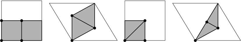
Figure 3: The four different $Z_{n}$ orbifold geometries in 6d, corresponding to $n=2,3,4,6$ (from left to right). We show the embedding of the orbifold fundamental domain (shaded) in the torus (thin line) as well as the fixed points (dots). The shaded regions have to be folded over the center line and the edges (thick lines) have to be identified. The resulting geometries are “pillows” with three or four corners. Note that the edges correspond to nonsingular bulk points.

The $Z_{n}$ rotation has to be represented on the fields and defines a Wilson line $P_{\mathcal{G}}$ around the fixed point located at the origin. In addition, one can allow for continuous or discrete Wilson lines associated to lattice translations [34]. However, geometric constraints apply. For instance, any lattice translations $T^{\lambda}$ (along some lattice vector $\lambda$) and discrete $Z_{n}$ rotation $P$ satisfy

$$PT^{\lambda}P^{-1}=T^{P\lambda}\,,\qquad T^{\lambda}T^{\lambda^{\prime}}=T^{\lambda^{\prime}}T^{\lambda}=T^{\lambda+\lambda^{\prime}}\,.$$ (4.1)

(Note that $P\lambda$ is another lattice vector). Both relations follow from elementary geometry in two dimensions. The representation of $T^{\lambda}$ on the fields (the torus Wilson line $T^{\lambda}_{\mathcal{G}}$) and the $Z_{n}$ Wilson line $P_{\mathcal{G}}$ around the origin then have to obey analogous constraints. As a matter of fact, if the torus Wilson lines are of finite order, $(T^{\lambda}_{\mathcal{G}})^{m}=1$, one can interpret the geometry as an orbifold of a larger torus with no Wilson lines on them [18]. The resulting orbifold group can be nonabelian, which then allows for rank reducing breakings of the gauge group [11, 35]. However, a simple solution to the constraints Eq. (4.1) consists of taking $P_{\mathcal{G}}$ to be an inner automorphism and choosing $T^{\lambda}_{\mathcal{G}}$ to lie in the Cartan torus as well. In that case we have $(T^{\lambda}_{\mathcal{G}})^{n}=1$ and the resulting orbifold group is Abelian.

We will refer to this description in terms of the covering torus and its Wilson lines as the upstairs picture. On the other hand, the maybe simpler and more physical approach is the downstairs picture in terms of the fundamental domain of the orbifold, i.e. the pillow geometries depicted in Fig. 3. To each of the corner singularities of these spaces one associates a Wilson line $P^{(f)}_{\mathcal{G}}$ corresponding to the rotation around that given fixed point which is a product of torus and $Z_{n}$ Wilson lines. The geometric constraints of the upstairs picture then translate into constraints onto the $P^{(f)}_{\mathcal{G}}$, for instance

$$\bigl{(}P^{(f)}_{\mathcal{G}}\bigr{)}^{n_{f}}=1\,,\qquad P^{(1)}_{\mathcal{G}}P^{(2)}_{\mathcal{G}}\cdots P^{(\nu)}_{\mathcal{G}}=1\,,$$ (4.2)

where $\nu$ is the number of fixed points and $n_{f}$ is the order of the fixed point. The ordering of the Wilson lines is counterclockwise along the corners of the pillow and cyclic permutations of the last identity hold. While the meaning of the first relation in Eq. (4.2) is obvious, the second identity has another simple geometric interpretation that is illustrated in Fig. 4.

Figure 4: Illustration of the second relation in Eq. (4.2) for the $Z_{2}$ pillow. If the path encloses the four corners of the space in a cyclic order, it becomes contractible and the associated Wilson line must be unity (the dashed lines represent parts of the path on the back side of the pillow).

If the $T^{\lambda}_{\mathcal{G}}$ commute with $P_{\mathcal{G}}$ the only additional constraints to Eq. (4.2) are that the $P_{\mathcal{G}}^{(i)}$ commute. For nonabelian orbifolds however, the downstairs constraints become more complicated. In the most general case, the $P_{\mathcal{G}}^{(i)}$ have to form a representation of the (nonabelian) fundamental group of the pillow space. We refer the reader to Ref. [11] for some possible generalizations of this downstairs construction that cannot be lifted to the upstairs picture.

In the downstairs picture it is particularly transparent that the compact torus orbifolds are locally equivalent to non-compact orbifolds and all one has to know for the physics of the fixed points are the local Wilson line one encounters by encircling the singularities. In particular, the localized anomaly is completely known from this local data.

We would like to perform a consistency check on the local Lorentz anomaly found in Sec. 3.2 by taking the compactification limit. To this end, consider first a torus compactification and take the limit of vanishing internal volume. Clearly the remnant local Lorentz symmetry is spontaneously broken, but in the limit where all heavy KK modes decouple it survives as a global symmetry. As can easily be checked, on the 4d zero modes of a 6d Weyl fermion this symmetry acts as a chiral $U(1)$:

$$\left(\begin{array}[]{c}\psi_{L}\\ \psi_{R}\end{array}\right)\to\exp\left(-\frac{i}{2}\Lambda_{45}\gamma^{5}\right)\left(\begin{array}[]{c}\psi_{L}\\ \psi_{R}\end{array}\right)\,.$$ (4.3)

Hence the spectrum of zero modes is not anomaly free but instead we find

$$\mathcal{A}_{L,tor}^{(0)}=2\cdot\frac{1}{8\pi^{2}}\Lambda_{45}\operatorname{Tr}A_{2}\,.$$ (4.4)

Note that this is unlike the case of gauge symmetries which always result in vector-like theories in 4d.

Now orbifold this model on $T^{2}/Z_{n}$. The Wilson lines around the singularities determine which of the two zero modes (if any) survives the projection. Let us – for simplicity – assume a $U(1)$ gauge symmetry. The expected zero mode anomaly is

$$\mathcal{A}_{L,orb}^{(0)}=n_{0}\cdot\frac{1}{8\pi^{2}}\Lambda_{45}\operatorname{Tr}A_{2}\,,$$ (4.5)

where the integer coefficient $n_{0}$ counts the number of zero modes (only $n_{0}=0,1$ occur). Note that the anomaly is the same independent of the chirality of the 4d zero mode. The localized local Lorentz anomaly, integrated over the compact dimension, should equal the difference of the zero mode anomaly for the chiral $U(1)$ between the orbifold and torus compactification:

$$\int\mathcal{A}_{L}=\mathcal{A}_{L,orb}^{(0)}-\frac{1}{n}\mathcal{A}_{L,tor}^{(0)}\,.$$ (4.6)

Eq. (4.6) can be checked from Eq. (3.33) directly for $n=2,3,4,6$ and for arbitrary $P_{\mathcal{G}}$. In particular, for $n=2$ there is always precisely one zero mode, independent of the Wilson line, implying that Eq. (4.6) gives zero in accordance with our analysis of Sec. 3.2.

5 Examples in Supersymmetric Theories

In this subsection we would like to illustrate our so far very abstract discussion with some examples that are possibly relevant to 6d supersymmetric orbifold GUTs. We will focus mainly on the irreducible gauge anomaly of type $\operatorname{Tr}F^{3}$ as it gives the most stringent restrictions on the localized spectrum. After commenting on the SUSY breaking features of a 6d orbifold fixed point, we will review 6d bulk anomaly cancellation conditions and finally apply the results of Sec. 3 to some interesting GUT gauge groups.

5.1 Supersymmetry breaking

The main success of orbifolds is their capacity to produce chiral boundary-conditions and spectra. Given that the orbifold breaks chirality it is not surprising that SUSY is also broken at an orbifold fixed point. Due to the presence of the $P_{L}$ factor in the orbifold twist particles acquire spin-dependent boundary conditions. Moreover, in general there is an additional explicit $R$-symmetry twist due to the fact that $(P_{L})^{n}=-1$ for fermions. For instance, while for gauge fields we have $(P_{\mathcal{G}})^{n}=+1$, for gauginos we actually need $(P_{\mathcal{G}})^{n}=-1$. One concludes that $P_{\mathcal{G}}$ has to include an additional-$R$ symmetry twist. How much SUSY is locally broken depends on the order $n$ of the fixed point as well as the form of the $R$-symmetry twist, as we will see shortly. The amount of global (low energy) SUSY breaking depends on the (mis)match of the supercharges locally preserved at different fixed points. The latter is generally referred to as Scherk-Schwarz (SS) SUSY breaking and is widely used in string and field theoretical models. To find the surviving supercharges at a given singularity, we have to look more closely at the $R$-symmetry. Pure $N=(1,0)$ supersymmetric gauge theory in 6d is invariant under an $SU(2)_{R}$ symmetry, which acts on gauginos only but not on the gauge fields. Gauginos are doublets under this symmetry and obey a symplectic Majorana constraint,

$$(\psi^{i})^{*}=\epsilon_{ij}C\psi^{j}\,,$$ (5.1)

where $C$ is the 6d charge conjugation matrix and $\epsilon_{ij}$ is the antisymmetric tensor of $SU(2)_{R}$. Without loss of generality we can choose the $R$ symmetry twist to be $\exp(2\pi i\,p_{R}/n\,\sigma_{3})$ with $p_{R}=r-1/2$. Eliminating $\psi^{2}$ with the help of the constraint Eq. (5.1), the remaining $\psi^{1}$ is simply twisted by a phase

$$P_{R}=\exp(2\pi i\,p_{R}/n)\,.$$ (5.2)

In terms of the 4d chiral spinors $\psi_{L}$ and $\psi_{R}$ (see App. A) the orbifold constraints on the gauginos of $\mathcal{H}$ imply

$$\psi_{L}(y=0) = \exp(2\pi i\,(r-1)/n)\,\psi_{L}(y=0)\,,$$

$$\psi_{R}(y=0) = \exp(2\pi i\,r/n)\,\psi_{R}(y=0)\,.$$ (5.3)

We see that for $r=0\mod n\ (r=1\mod n)$ it is $\psi_{R}\ (\psi_{L})$ that locally survives the projection, leading to $N=1$ unbroken SUSY. For any other value of $r$ both 4d gauginos vanish, implying complete breakdown of SUSY. For later purposes let us introduce the periodic Kronecker symbol $\delta_{r,n}$ which by definition equals one for $r=0\mod n$ and zero otherwise. The amount of 4d supersymmetry at the fixed point can then be expressed as

$$N=\delta_{r,n}+\delta_{r-1,n}\,.$$ (5.4)

One sees that $n=2$ fixed points always have $N=1$ supersymmetry, while for $n>2$ one can have $N=1$ or $N=0$. Note that in the $Z_{4}$ and $Z_{6}$ compact orbifolds there is actually a $Z_{2}$ fixed point present. This means that locally some SUSY survives in these cases.

Let us now introduce matter hypermultiplets. The $R$-symmetry twist acts on the hyperscalars only, implying that we now need $(P_{\mathcal{G}})^{n}=-1$ for the multiplet as a whole. In general, this requires additional Wilson lines for matter fields. We will see some examples in Sec. 5.3. It is important to check that any symmetry used in orbifolding is anomaly free in the unorbifolded theory [15]. For the $SU(2)_{R}$ twist(s) this is trivially the case. If the additional Wilson lines in the matter sector involve $U(1)$’s, this may provide further constraints.

Next, we would like to comment on models with extended $N=(N_{+},N_{-})$ SUSY. The $R$-symmetry group is $U\!Sp(2N_{+})\otimes U\!Sp(2N_{-})$ [37]. In particular, for the case of $N=(1,1)$ SUSY, it is $SU(2)_{R}\otimes SU(2)_{R}^{\prime}$. The (say) left handed vector multiplet is paired up with a right handed adjoint hypermultiplet to form a complete $N=(1,1)$ vector multiplet. With respect to the second $SU(2)_{R}^{\prime}$, the vector multiplet is a singlet and the hypermultiplet a doublet obeying the reality constraints

$$(H^{a}_{i})^{*}=\epsilon_{ab}\epsilon^{ij}H_{j}^{b}\,\qquad(\psi^{a})^{*}=\epsilon_{ab}C\psi^{b}\,.$$ (5.5)

Without loss of generality we can choose the $SU(2)_{R}^{\prime}$ twist to be proportional to $\sigma_{3}$ and eliminate the $a=2$ components of the hypermultiplet with the above constraint. The action of the total $R$ symmetry twist on $\psi^{1}$ can then be parametrized as

$$P_{R}^{\prime}=\exp(2\pi ip_{R}^{\prime}/n)\,,\qquad p_{R}^{\prime}=r^{\prime}-\frac{1}{2}\,.$$ (5.6)

The amount of supersymmetry surviving at the fixed points can again be computed by determining the non-vanishing fields at the singularity. It turns out to be

$$N=\delta_{r,n}+\delta_{r^{\prime},n}+\delta_{r-1,n}+\delta_{r^{\prime}-1,n}\,.$$ (5.7)

One sees that for $n=2$ only $N=2$ occurs, while for $n>2$ we can break down to $N=2$, $N=1$ and $N=0$. This has lead people to consider $n>2$ orbifolds [9]. However as far as low energy supersymmetry is concerned one can achieve $N=1$ on a $Z_{2}$ orbifold by invoking the SS mechanism.

5.2 Bulk anomaly cancellation

In this subsection we compute anomaly free spectra in 6 spacetime dimensions. We will focus here on the irreducible gauge anomaly only, that is the nonfactorizable trace of four generators. In addition, the cancellation of the irreducible gravitational anomaly has to be enforced. Besides spin $1/2$ fermion, there are contributions to the irreducible gravitational anomaly from gravitinos and (anti) self-dual tensor fields. Finally, the reducible anomalies, e.g. $(\operatorname{Tr}F^{2})^{2}$ or $\operatorname{Tr}R^{2}\operatorname{Tr}F^{2}$, can be canceled by the GS-mechanism involving two-forms,[32] and do not place any restrictions on the 6d fermion spectrum. For previous work on 6d anomaly cancellation see Refs. [38, 17, 6].

The simplest GUT group, $SU(5)$, does not lead to nontrivial chiral 6d spectra. The reason is that 6d matter hypermultiplets have to carry opposite chirality w.r.t. the gaugino (See, e.g., the discussion in [39]). Furthermore, complex conjugation does not flip the chirality of a 6d spinor, in contrast to the 4d case. In accordance with this $\operatorname{Tr}F^{4}$ is the same for a representation and its conjugate. Cancellation of the irreducible part of the gauge anomaly requires the following identities for $SU(5)$:

$$\operatorname{Tr}_{\bf 24}F^{4} = 10\operatorname{Tr}_{\bf 5}F^{4}+6(\operatorname{Tr}_{\bf 5}F^{2})^{2}\,,$$

$$\operatorname{Tr}_{\bf 10}F^{4} = -3\operatorname{Tr}_{\bf 5}F^{4}+3(\operatorname{Tr}_{\bf 5}F^{2})^{2}\,,$$

$$\operatorname{Tr}_{\bf 15}F^{4} = 13\operatorname{Tr}_{\bf 5}F^{4}+3(\operatorname{Tr}_{\bf 5}F^{2})^{2}\,,$$ (5.8)

We thus conclude that with fundamental and antisymmetric representations alone no “economic” anomaly free models are possible: 6d anomaly cancellation requires in fact no less than 10 fundamentals. The simplest nontrivial solutions would be an antisymmetric (${\bf 10}$) and a symmetric (${\bf 15}$) or an adjoint multiplet of opposite chirality. The latter of course leads to a vector-like theory in 6d. As for the former solution note that the quarks contained in the symmetric and antisymmetric representations and the ones in the adjoint have incompatible hypercharges. This means that one has to project out one of them by orbifolding.

In fact these two solutions generalize to $SU(N)$, as the $SU(5)$ relations Eq. (5.8) have a straightforward generalization

$$\operatorname{Tr}_{\bf r}F^{4}=c_{4}\operatorname{Tr}_{N}F^{4}+c_{2}\operatorname{Tr}_{N}(F^{2})^{2}\,,$$ (5.9)

with $c_{4}=2N,N+8,N-8$ and $c_{2}=6,3,3$ for the adjoint, symmetric tensor and antisymmetric tensor representations respectively.

In the $SO(10)$ case there do exist interesting anomaly free 6d spectra as can be seen from the relations

$$\operatorname{Tr}_{{\bf 45}}F^{4} = 2\operatorname{Tr}_{\bf 10}F^{4}+3(\operatorname{Tr}_{\bf 10}F^{2})^{2}\,,$$ (5.10)

$$\operatorname{Tr}_{{\bf 16}}F^{4} = -\operatorname{Tr}_{\bf 10}F^{4}+\frac{3}{4}(\operatorname{Tr}_{\bf 10}F^{2})^{2}\,,$$ (5.11)

The minimal matter content would thus consist of two ${\bf 10}$ hypermultiplets in the bulk, while further ${\bf 10}$’s and ${\bf 16}$’s should occur in pairs. Finally, $E_{6}$, $E_{7}$ and $E_{8}$ do not have any independent fourth order invariants and thus the adjoint representation (as any other representation) does not have an irreducible bulk anomaly.

5.3 Localized anomaly cancellation

Since the fixed points are four-dimensional, only $SU(N)$ factors of $\mathcal{H}$ will potentially contribute to the irreducible gauge anomaly. We will convert all anomalies to the fundamental, i.e. we will express everything in terms of the quantities

$$I_{N}\equiv\operatorname{Tr}_{N}F^{3}\,.$$ (5.12)

For $\mathcal{G}=SU(5)$, let us fix the matter content to an adjoint hypermultiplet of opposite chirality w.r.t. the gauge multiplet. The local breaking to the standard model is achieved by deleting the third (equivalently second) node of the Dynkin diagram, which is accomplished by the shift vector

$$V=\frac{1}{n}\,\mu^{(3)}\,.$$ (5.13)

The ${\bf 24}$ branching rule is given by

$${\bf 24}\to({\bf 3},{\bf 2})_{1}\oplus({\bf\overline{3}},{\bf 2})_{-1}\oplus{\bf adj}({\rm SM})\,,$$ (5.14)

where the generator of the $U(1)$ is given by $nV=\mu^{(3)}$. As explained in the Sec. 5.1, we need to multiply this gauge twist by an $R$-symmetry twist Eq. (5.2). For the matter hypermultiplet an additional phase $\exp(2\pi ip_{M}/n)$ with $p_{M}=m-1/2$ has to be added. This can be embedded in a matter $U(1)$, which is non anomalous in the 6d unorbifolded theory as the trace over three adjoint generators vanishes. However, since this system is actually $N=(1,1)$ supersymmetric, we can also interpret $p_{M}$ as the other $R$ symmetry twist $p_{R}^{\prime}$ (see Sec. 5.1) and identify $m$ with $r^{\prime}$. Following Sec. 3.1 one finds that the gaugino contributes

$$\tilde{I}_{{\bf 24}}=\left(-\frac{1}{n}-\frac{p_{R}}{n}+\left\lfloor 1/n+p_{R}/n\right\rfloor\right)I_{{\bf 3}}\\ +\left(\frac{1}{n}-\frac{p_{R}}{n}+\left\lfloor-1/n+p_{R}/n\right\rfloor\right)I_{\bf\overline{3}}$$ (5.15)

As before, $\left\lfloor x\right\rfloor$ stands for the floor function defined as the closest integer $k\leq x$. The two floor functions cancel unless $r=0,1\mod n$ (in which case they give unity), hence

$$\tilde{I}_{{\bf 24}}=2\left(-\frac{2}{n}+\delta_{r,n}+\delta_{r-1,n}\right)I_{{\bf 3}}\,,$$ (5.16)

where the Kronecker-$\delta$ has again to be continued periodically. The matter multiplet contributes $-\tilde{I}_{\bf 24}$ with $r$ replaced by $r^{\prime}$, hence

$$\tilde{I}_{\bf 24}-\tilde{I}_{\bf 24^{\prime}}=2\left(\delta_{r,n}+\delta_{r-1,n}-\delta_{r^{\prime},n}-\delta_{r^{\prime}-1,n}\right)I_{{\bf 3}}\,.$$ (5.17)

The fractional parts cancel as expected and the remaining $SU(3)$ anomaly has an integer coefficient. Note that the inflow terms are zero since the adjoint is a real representation. We can see that if the anomaly is non-vanishing it carries a coefficient 2, so that the localized matter content has to be either one quark doublet $({\bf 3},{\bf 2})$ or two quark singlets $({\bf 3},{\bf 1})$. Which of the quarks doublets contained in the ${\bf 24}$ have zero modes upon compactification depends on the Wilson lines at the other fixed points. An interesting model based on $T^{2}/Z_{3}$ can be constructed as follows: Break $SU(5)$ to the standard model with the gauge twist Eq. (5.13) and supersymmetry to $N=1$ with the $R$-symmetry twist $r=0$ and $r^{\prime}=2$ at all three fixed points. This produces three quark doublets $({\bf 3},{\bf 2})_{1}$ from bulk zero modes, whose anomaly is distributed uniformly over the three fixed points. The model can then trivially be made anomaly free by completing the generations at each of the fixed points. Of course, Higgs fields have to be added to the model. However, there does not exist a simple $SU(5)$ representation that contains $SU(2)$ doublets with the correct hypercharge w.r.t. to the quark doublets, and, hence, the Higgs sector should reside on a brane. On the other hand, this forbids some of the Yukawa couplings, which, in addition, cannot be generated radiatively. One probably has to extend the gauge group to $SU(6)$ to include a realistic Higgs sector in the model. A similar model has been developed in Ref. [10] with $SO(10)$ as a gauge group and Higgs fields at one of the fixed points. However apart from the problem of how to generate Yukawa interactions for two generations, that model requires an additional mechanism to break the remaining $SU(5)$ and in particular also suffers from the same doublet triplet splitting problem as conventional 4d GUT models. Other – less symmetric – constructions are certainly possible, perhaps with the quark doublets of only one or two generations originating from the bulk. Note that there is no localized anomaly from the gauginos on fixed points with unbroken $SU(5)$, hence one can always introduce complete generations $({\bf 10},{\bf\overline{5}})$ there.

Next, consider $\mathcal{G}=SO(10)$, which has been studied extensively in the context of orbifold GUTs in [8, 9, 17, 10, 40]. Let us start with the breaking pattern $SO(10)\to SU(5)\otimes U(1)$ which can be achieved by deleting the fourth or fifth node of the Dynkin diagram [11], see Fig.1. It thus corresponds to the shift vector

$$V=\frac{1}{n}\,\mu^{(4)}\,.$$ (5.18)

The branching rules of the various low-dimensional representations read as follows.

$${\bf 45} \to {\bf 1}_{0}\oplus{\bf 10}_{1}\oplus{\bf\overline{10}}_{-1}\oplus{\bf 24}_{0}\,,$$ (5.19)

$${\bf 10} \to {\bf 5}_{1/2}\oplus{\bf\overline{5}}_{-1/2}\,,$$ (5.20)

$${\bf 16} \to {\bf 1}_{-5/4}\oplus{\bf\overline{5}}_{3/4}\oplus{\bf 10}_{-1/4}\,.$$ (5.21)

Looking at the charges occurring in these branching rules, we see that $n\,V_{\bf 10}=1/2$ and $n\,V_{\bf 16}=3/4$ (modulo integers). One concludes that the ${\bf 16}$ has to have an additional orbifold phase $p_{M}=m-1/4$. The latter can be introduced without problems, since it can be embedded in an anomaly free global $U(1)_{M}$ under which only the ${\bf 16}$ is charged. One can also include an additional phase $p_{M}=m$ for the ${\bf 10}$ in order to account for further local or global Wilson lines. Let us now focus on the possible irreducible gauge anomaly at the 4d fixed point, that is the $SU(5)^{3}$ anomaly. Normalizing to the fundamental of $SU(5)$ one finds

$$\tilde{I}_{{\bf 45}}=\left(-\frac{2}{n}+\delta_{r,n}+\delta_{r-1,n}\right)I_{{\bf 5}}\,.$$ (5.22)

In a similar fashion, we find for the ${\bf 10}$ and ${\bf 16}$

$$\tilde{I}_{{\bf 10}}=\left(-\frac{1}{n}+\delta_{m,n}\right)I_{{\bf 5}}\,,\qquad\tilde{I}_{{\bf 16}}=\tilde{I}_{{\bf\overline{16}}}=\left(\frac{1}{n}-\delta_{m,n}\right)I_{{\bf 5}}\,.$$ (5.23)

Adding the contribution of a (say) left handed gaugino and two right handed matter multiplets ${\bf 10}$ and ${\bf 10^{\prime}}$, the bulk anomaly is canceled. As it must be, this fermion content also cancels the non-integer coefficient of the $I_{{\bf 5}}$ as it is directly linked to the 6d anomaly. The total anomaly

$$\tilde{I}_{{\bf 45}}-\tilde{I}_{{\bf 10}}-\tilde{I}_{{\bf 10^{\prime}}}=(\delta_{r,n}+\delta_{r-1,n}-\delta_{m,n}-\delta_{m^{\prime},n})I_{{\bf 5}}\,.$$ (5.24)

again depends on the $R$-symmetry and matter phases. It vanishes for certain combinations of $r$, $m$ and $m^{\prime}$. For instance in the $n=2$ model of Ref. [8, 17] it was assumed that the ${\bf 10}$ had positive parity ($m=0$) and the ${\bf 10^{\prime}}$ negative ($m^{\prime}=1$) and hence no anomaly occurs. In this case it turns out that the local spectrum is anomaly free for both $r=0,1$. On the other hand consider an $n=4$ fixed point and the assignments $r=0$, $m=0$ and $m^{\prime}=2$. Still the localized anomaly vanishes, but it is not hard to check that the local spectrum consists of one ${\bf 10}$ and two ${\bf\overline{5}}$, which would not be anomaly free. This example shows that one in general cannot determine the localized anomaly from the knowledge of the local spectrum. Finally notice that the localized anomaly of pairs of $({\bf 10},{\bf 16})$ or $({\bf 10},{\bf\overline{16}})$ again has no fractional coefficient.

The orbifold twist

$$V=\frac{1}{2}\mu^{(2)}$$ (5.25)

leaves the Pati Salam (PS) group $SU(4)\otimes SU(2)\otimes SU(2)$ unbroken. The corresponding branching rules read

$${\bf 45} \to ({\bf 6},{\bf 2},{\bf 2})\oplus{\bf adj}(\rm PS)\,,$$

$${\bf 10} \to ({\bf 6},{\bf 1},{\bf 1})\oplus({\bf 1},{\bf 2},{\bf 2})\,,$$

$${\bf 16} \to ({\bf 4},{\bf 2},{\bf 1})\oplus({\bf\overline{4}},{\bf 1},{\bf 2})$$ (5.26)

The localized anomaly has been discussed in the context of the model of Ref. [17], we include it here for the sake of completeness. As the ${\bf 6}$ is a real representation of $SU(4)$, it does not have a 4d anomaly. Hence the only contribution can come from the ${\bf 16}$. The phases for the ${\bf 4}$ and ${\bf\overline{4}}$ turn out to be $V_{{\bf 4}}=1/2$ and $V_{{\bf\overline{4}}}=0$. To this, one has to add a matter phase $p_{M}=m-1/2$. From Eq. (3.23) one finds for the localized anomaly

$$-\tilde{I}_{{\bf 16}}=\frac{1}{2\pi i}\left(\log^{\prime}[e^{2\pi i(\frac{1}{2}+\frac{m}{2}-\frac{1}{4})}]-\log^{\prime}[e^{2\pi i(\frac{m}{2}-\frac{1}{4})}]\right)2I_{\bf 4}=(-1,1)I_{\bf 4}\,$$ (5.27)

where the two coefficients refer to $m=0,1$ respectively. We observe that unless further pairs of $({\bf 10},{\bf 16})$ are introduced in the bulk, one always needs to add at least a single $({\bf 4},{\bf 1},{\bf 1})$ or $({\bf\overline{4}},{\bf 1},{\bf 1})$ at the fixed point. This could possibly correspond to a left handed quark in realistic orbifold constructions.

Next we turn to $\mathcal{G}=E_{6}$. As mentioned before, $E_{6}$ does not have an irreducible 6d gauge anomaly. Furthermore, like for $SO(10)$, the trace over three generators vanishes so there cannot be any anomaly inflow from the bulk to the fixed point. Let us consider the shift vector

$$V=\frac{1}{3}\mu^{(3)}\,.$$ (5.28)

This eliminates the third node of the Dynkin diagram but projects in the highest root $\theta$. The resulting gauge group is $SU(3)\otimes SU(3)^{\prime}\otimes SU(3)^{\prime\prime}$ where $\alpha^{(1,2)}$ serve as simple roots for $SU(3)$, $\alpha^{(4,5)}$ for $SU(3)^{\prime}$ and $\alpha^{(6)}$ and $-\theta$ for $SU(3)^{\prime\prime}$. The branching of the adjoint is given by

$${\bf 78} \to ({\bf\overline{3}},{\bf 3},{\bf 3})\oplus({\bf 3},{\bf\overline{3}},{\bf\overline{3}})\oplus{\bf adj}$$ (5.29)

$$\to ({\bf\overline{3}},{\bf 3},{\bf 2})_{-1}\oplus({\bf\overline{3}},{\bf 3},{\bf 1})_{2}\oplus({\bf 3},{\bf\overline{3}},{\bf 2})_{1}\oplus({\bf 3},{\bf\overline{3}},{\bf 1})_{-2}\oplus\dots\,,$$

where in the second line we have indicated the breaking of $SU(3)^{\prime\prime}$. From the charges it is clear that $V_{{\bf\overline{3}}{\bf 33}}=2/3$ and $V_{{\bf 3}{\bf\overline{33}}}=1/3$ (modulo integers). One finds

$$\tilde{I}_{\bf 78} = (3,3,-6)(I_{\bf 3}-I^{\prime}_{\bf 3}-I^{\prime\prime}_{\bf 3})\,,$$ (5.30)

where the coefficients refer to the values $r=(0,1,2)$. For $r=0,1$ (corresponding to $N=1$ supersymmetry at the fixed point, see Sec. 5.1), the minimal localized matter content that cancels the localized anomaly is given by $3\times({\bf\overline{3}},{\bf 1},{\bf 1})$ and $1\times({\bf 1},{\bf 3},{\bf 3})$, or $3\times({\bf 1},{\bf 3},{\bf 1})$ and $1\times({\bf\overline{3}},{\bf 1},{\bf 3})$, or $3\times({\bf 1},{\bf 1},{\bf 3})$ and $1\times({\bf\overline{3}},{\bf 3},{\bf 1})$. Let us identify the first $SU(3)$ with color and the second with $SU(3)_{W}\supset SU(2)_{W}$. Ignoring the $U(1)$ charges for a moment, one sees that e.g. the first choice provides three generations of leptons and quark singlets. The missing fields have to either reside on other fixed points or come from bulk zero modes. For the latter possibility notice that the only bulk field that is nonvanishing at the fixed point is a $({\bf 3},{\bf\overline{3}},{\bf\overline{3}})$. Provided it is nonvanishing at the other fixed points as well and, thus, has a zero mode, it precisely gives rise to the missing quarks. In any event, one has to find a suitable $U(1)$ subgroup of $SU(3)_{W}\otimes SU(3)^{\prime\prime}$ that can act as hypercharge and is in particular free of localized anomalies. Building a concrete orbifold model containing such a particular local GUT breaking at one of its fixed points is beyond the scope of the present paper and is left to future research.

As a last example consider the breaking of $E_{7}$ to $SU(5)\otimes SU(3)\otimes U(1)$ accomplished by the shift vector

$$V=\frac{1}{n}\mu^{(4)}\,,\qquad n>3\,.$$ (5.31)

(For $n=3$ the gauge group is actually enhanced to $SU(6)$). The adjoint of $E_{7}$ is the ${\bf 133}$ and has the following branching rule:

$${\bf 133}\to({\bf 10},{\bf\overline{3}})_{1}\oplus({\bf 5},{\bf\overline{3}})_{-2}\oplus({\bf\overline{10}},{\bf 3})_{-1}\oplus({\bf\overline{5}},{\bf 3})_{2}\oplus({\bf 5},{\bf 1})_{3}\oplus({\bf\overline{5}},{\bf 1})_{-3}\oplus{\bf adj}\,.$$ (5.32)

For instance, for $r=0,1$ (the $R$ symmetry twist that preserves $N=1$ supersymmetry) we find for the anomaly

$$\tilde{I}_{\bf 133}=I_{\bf 5}-5I_{\bf 3}\,,$$ (5.33)

for any $n>3$. It turns out that at least three irreducible representations are necessary to cancel this anomaly. The possibilities are a $({\bf\overline{5}},{\bf 3})$ and two $({\bf 5},{\bf 1})$ (one or both of which can also be replaced by $({\bf 10},{\bf 1})$) or a $({\bf 10},{\bf 3})$, a $({\bf\overline{5}},{\bf\overline{3}})$ and a $({\bf 5},{\bf 1})$. The latter exactly gives three generations of quarks and leptons plus an additional ${\bf 5}$ which could serve as one of the Higgses. Once again, including more matter fields in the bulk (in particular extending bulk supersymmetry) changes the localized anomaly and hence these predictions. For a model with $N=(1,1)$ supersymmetry and this particular breaking pattern see Ref. [11].

We can see from the last two examples that if the unbroken subgroup contains two or more nonabelian factors that have cubic anomalies in 4d, the localized anomaly cancellation condition can be quite restrictive. Some (incomplete) list of breakings of the exceptional groups and their anomalies is presented in Tab. 1

Shift Vector	Breaking	Gaugino Anomaly $\tilde{I}_{\bf adj}$
$\mu^{(2)}/2$	$E_{6}\to SU(6)\otimes SU(2)$	0
$\mu^{(3)}/3$	$E_{6}\to SU(3)\otimes SU(3)^{\prime}\otimes SU(3)^{\prime\prime}$	$3(I_{\bf 3}-I^{\prime}_{\bf 3}-I^{\prime\prime}_{\bf 3})$
$\mu^{(2)}/3$	$E_{7}\to SU(6)\otimes SU(3)$	$-5I_{\bf 3}+2I_{\bf 6}$
$\mu^{(7)}/2$	$E_{7}\to SU(8)$	0
$\mu^{(4)}/5$	$E_{8}\to SU(5)\otimes SU(5)^{\prime}$	$I_{\bf 5}-7I^{\prime}_{{\bf 5}}$
$\mu^{(6)}/3$	$E_{8}\to E_{6}\otimes SU(3)$	$9I_{\bf 3}$
$\mu^{(8)}/3$	$E_{8}\to SU(9)$	$-3I_{\bf 9}$

Table 1: The localized anomaly for different breakings of the exceptional groups $E_{6,7,8}$. Note the anomaly vanishes in 4d if the adjoint branches exclusively into real representations of the unbroken group. It is assumed that $N=1$ supersymmetry is preserved $(r=0,1)$.

6 Conclusions

In this paper we have analyzed the occurrence of localized anomalies on fixed points of orbifolds of 4+2 dimensional smooth spacetimes. Such fixed points constitute conical singularities obtained by gluing together the edges of the “wedge” $\{r,\theta\}$, the angle theta taking values $0\leq\theta\leq 2\pi/n$. Internal (global or local) symmetries can be broken by this procedure by identifying the 6d fields on the two edges only up to an orbifold twist (Wilson line).

We have shown that the pure gauge anomaly of the unbroken group $\mathcal{H}\subset\mathcal{G}$ caused by a 6d Weyl fermion can be interpreted as coming from a background field configuration that would be obtained by gauging away the orbifold twist. This particular form led us to a natural splitting of the anomaly localized at the 4d fixed point into three terms

$$-\operatorname{Tr}(VF^{3})+\operatorname{Tr}(\left\lfloor V\right\rfloor F^{3})+\frac{1}{2}\operatorname{Tr}(F^{3})$$ (6.1)

where $V$ is the so-called twist vector characterizing the orbifold twist (an element of the Cartan torus of the algebra) and $\left\lfloor x\right\rfloor$ denotes the closest integer $\leq x$. From this expression one can derive important consequences for the 4d irreducible (i.e. nonabelian) anomaly. We have shown that, once the 6d irreducible bulk anomaly is canceled, the first term does not contribute to the nonabelian 4d anomaly. On the other hand, the last term might be canceled by a 6d Green-Schwarz four-form (or its dual, an axion). Of course, it can also be canceled amongst fermions, for instance if a vector-like 6d fermion content is chosen. The term is nonzero only for $\mathcal{G}=SU(N)$ and vanishes even there if the fermion transforms in a real representations. The second term is a purely four-dimensional irreducible anomaly that can only be removed with the introduction of appropriate localized fermions at the singularity. Contrary to the other two terms, its coefficient is an integer, which is a necessary condition for local anomaly cancellation to occur. We have presented numerous examples in the context of supersymmetric orbifold GUTs.

We have also calculated the localized anomaly of 6d Lorentz symmetry and general covariance. To this end we have identified the remnants of the 6d gravitational symmetries at the 4d fixed point located at $y_{f}$ besides the corresponding 4d ones. In terms of the 6d parameters $\Lambda_{AB}(x,y)$ and $\xi^{M}(x,y)$ they are generated by $\Lambda_{ab}(x,y_{f})$, $\partial_{m}\xi^{m}(x,y_{f})$ and $\partial_{[m}\xi_{n]}(x,y_{f}))$. We find that only the first and second symmetries have localized anomalies. While the scaling symmetry $\partial_{m}\xi^{m}$ can be rendered consistent by adding suitable local counterterms to the action, quantum consistency of the remnant Lorentz symmetry $U(1)_{L}$ requires that localized fields are charged under it. This is rather surprising from a field theory point of view, but occurs naturally in string theory orbifolds. The localized fields of the low energy limit correspond to zero modes of twisted strings. The latter do in fact transform non-trivially under $U(1)_{L}$ (or, more general under $SO(6)$) and hence are expected to contribute to the anomaly.

Let us conclude by pointing out some interesting directions of further research. Clearly, most of our findings can more or less directly be generalized to any codimension-two orbifold-singularity. Of course, the structure of the $d-2$ dimensional anomalies is different, but our general findings for the gauge anomalies will not change. Another interesting direction concerns codimension-two conical singularities of opening angles other than $2\pi/n$ and gauge twists whose order is unrelated to the geometric twist [11]. The fact that our results are independent of $n$ and only depend on the $\delta$-function like background flux $\left\langle F\right\rangle$ points towards similar results in these cases. On the technical side however, our calculation crucially depended on the ability to define our theory on a simply connected smooth covering space (with some constraints on the fields) which is no longer possible, even for rational opening angles such as $2\pi p/q$. Other, more refined tools are necessary, for instance the form of the heat kernel on arbitrary conical singularities (see Ref. [41]). The third obvious generalization concerns orbifold singularities of codimension other than two. Although higher dimensional analogues of the finite sums in App. C can be performed and yield similar polynomials in the logarithm of the orbifold twist, the immediate consequences for anomaly cancellation tend to be more involved than in the codimension-two case. The remnant local Lorentz symmetry at the singularity becomes a nonabelian one and one expects more stringent restrictions on the localized matter content to achieve anomaly cancellation.

Appendix A Notations and Conventions

We will adopt the follwoing index convention: lower case greek letters take values $0\dots 3$, lower case latin letters $4\dots d-1$ and capital latin letters take values $0..d-1$. Moreover, letters from the beginning of the alphabet ($A,B,a,b,\alpha,\beta$) are flat space (Lorentz) indices, while letters from the middle of the alphabet ($M,N,m,n,\mu,\nu$) denote curved (Einstein) indices. Furthermore we will denote the extra dimenisonal coordinates with $y$ (i.e. $y_{1}=x_{4},\ y_{2}=x_{5}$) and often choose our coordinates such that the fixed point under consideration lies at $y=0$.

We will work in the Euclidean. Our $d$ dimensional $\Gamma$ matrices satisfy the Clifford algebra

$$\{\Gamma^{A},\Gamma^{B}\}=2\delta^{AB}\,.$$ (A.1)

In $d=6$ we write this algebra in terms of the four-dimensional $\gamma$ matrices:

$$\Gamma^{a}=\gamma^{a}\otimes\sigma^{3},\qquad\Gamma^{4}=1\otimes\sigma^{1},\qquad\Gamma^{5}=1\otimes\sigma^{2}\,,$$ (A.2)

and we apply this construction recursively for higher dimensions. The $SO(d)$ generators are given by

$$J^{AB}=\frac{i}{4}[\Gamma^{A},\Gamma^{B}]\,.$$ (A.3)

The four-dimensional chirality matrix $\gamma^{5}$ is defined as $\gamma^{5}=\gamma^{0}\cdots\gamma^{3}=\operatorname{diag}(+1,+1,-1,-1)$. The $d$ dimensional chirality matrix (the analogue of $\gamma^{5}$) is defined as

$$\Gamma=\gamma^{5}\otimes\sigma^{3}\otimes\sigma^{3}\otimes\dots$$ (A.4)

The convention for the totally antisymmetric $SO(d)$ tensor is $\epsilon^{0\cdots d-1}=+1$

The particular choice for the $\Gamma$-matrices leads to a trivial embedding of $SO(4)$ spinor representations into $SO(d)$ ones:

$$J^{\alpha\beta}_{\Gamma}=\left(\begin{array}[]{ccc}J_{\gamma}^{\alpha\beta}&&\\ &J_{\gamma}^{\alpha\beta}&\\ &&\ddots\end{array}\right)\,,$$ (A.5)

where the subscript indicates the Clifford algebra matrices used to compute Lorentz-generators according to Eq. (A.3). Finally, in $d=6$ the generator for rotation in the $45$-plane is given by

$$\frac{1}{2}\Lambda^{ab}J_{ab}=\Lambda^{45}J_{45}=-\Lambda^{45}\frac{\sigma_{3}}{2}\,.$$ (A.6)

where $\Lambda_{45}$ is the angle of rotation.

Appendix B The Evaluation of the Heat Kernel

The object formally defined as

$$K(x,x^{\prime},s)\equiv\langle x|\exp(-s\Delta)|x^{\prime}\rangle$$ (B.1)

is called the Heat Kernel of the Laplace type differential operator $\Delta$. It satisfies the heat equation (hence the name)

$$\frac{\partial}{\partial s}K(x,x^{\prime},s)=-\Delta K(x,x^{\prime},s)\,,$$ (B.2)

obeying the boundary condition

$$K(x^{\prime}x^{\prime},0)=\delta(x,x^{\prime})\,,$$ (B.3)

where $\delta(x,x^{\prime})$ denotes the delta funcion (density) in curved space. The heat kernel appears in the calculation of anomalies, Eq. (3.2) with $\Delta$ the square of the Dirac operator,

$$\Delta=-D^{2}\!\!\!\!\!\!/\ =-D^{2}+E\,,\qquad E=-\frac{1}{4}R+\frac{i}{2}\Gamma^{MN}F_{MN}\,.$$ (B.4)

The covariant derivative on the right hand side of Eq. (B.4) contains spin, Christoffel and gauge connections, $F_{MN}$ stands short for $F_{MN}^{a}T_{a}$ with the hermitian generators $T_{a}$ and $R$ is the scalar curvature. Follwing deWitt [42] we write $K(x,x^{\prime},s)$ as a power series in the parameter $s$:

$$K(x,x^{\prime},s)\equiv(4\pi s)^{-d/2}D^{1/2}(x,x^{\prime})\exp(-\sigma(x,x^{\prime})/2s)\sum_{r\geq 0}a_{r}(x,x^{\prime})s^{r}\,.$$ (B.5)

The quantity $\sigma(x,x^{\prime})$ is called the geodesic biscalar and satisfies the differential equation

$$\frac{1}{2}\sigma_{;}^{M}\sigma_{;M}=\sigma\,,$$ (B.6)

where the semicolon denotes covariant differentiation w.r.t. $x$. The correspondig boundary condition reads

$$[\sigma](x)\equiv\sigma(x,x)=0\,.$$ (B.7)

From here on the brackets denote the coincidence limit $x^{\prime}=x$. $\sigma$ is a biscalar function whose magnitude equals half the geodesic distance squared between $x$ and $x^{\prime}$. It is the generalization of $(x-x^{\prime})^{2}/2$ in flat space. The following coincidence limits hold for $\sigma$

$$[\sigma_{;M}]=0\,,\qquad[\sigma_{;MN}]=g_{MN}\,,\qquad[\sigma_{;MNR}]=0\,.$$ (B.8)

Further coincidence limits can be obtained by repeated covariant differentiation of Eq. (B.6). The other quantity appearing in the ansatz Eq. (B.5) is the van Vleck-Morette determinant defined by the differential equation

$$D^{-1}(D{\sigma_{;}}^{M})_{;M}=d\,,$$ (B.9)

together with the boundary condition

$$[D]=\det g_{MN}\equiv g\,.$$ (B.10)

The normalization in Eq. (B.5) as well as the limit $[a_{0}]=1$ are chosen such as to correctly reproduce the boundary condition, Eq. (B.3). In other words

$$\lim_{s\to 0}\biggl{\{}(4\pi s)^{d/2}D(x,x^{\prime})^{1/2}\exp(-\sigma(x,x^{\prime})/2s)\biggr{\}}=\delta(x,x^{\prime})\,.$$ (B.11)

Inserting the ansatz Eq. (B.5) in the heat equation (B.2), one obtains the recursion relations

$${\sigma_{;}}^{M}a_{0;M}=0\,,$$ (B.12)

$${\sigma_{;}}^{M}a_{r;M}+r\,a_{r}=D^{-1/2}{(D^{1/2}a_{r-1})_{;M}}^{M}-E\,a_{r-1}\,.$$ (B.13)

From these relations and their covariant derivatives one can obtain the coincidence limits $[a_{r}]$ in a completely straightforward (but for higher $r$ increasingly tedious) manner. The $[a_{r}]$ are local covariant functionals of the curvature and field strength tensors and of their covariant derivatives (for details on the calculation see Ref. [42]).

To find the anomaly, Eq. (3.2), we need to calculate

$$\lim_{s\to 0}\lim_{x^{\prime}\to x}Q(x,x^{\prime\prime})K(x^{\prime\prime},x^{\prime},s)\,.$$ (B.14)

As mentioned in Sec. 3, the term proportional to the identity in $Q$ gives rise to the one $n$th the $d$ dimensional bulk anomaly, while the other terms produce brane anomalies. They are proportional to

$$K^{(k)}(x)\equiv\lim_{s\to 0}\lim_{x^{\prime}\to P^{k}x}K(x,x^{\prime},s)\,.$$ (B.15)

Clearly, unless $x=Px$, that is at the fixed point $y=0$, this quantity is exponentially suppressed in the limit $s\to 0$ while it diverges for $y=0$. We thus expect $K^{(k)}(x)$ to be a distribution centered at $y=0$. Indeed, one can calculate

$$\lim_{s\to 0}\ \left(\frac{D(x,P^{k}x)}{(4\pi s)^{m}}\right)^{\frac{1}{2}}\exp(-\sigma(x,P^{k}x)/2s)=\tilde{g}^{1/2}\,\nu_{k}^{-1}\,\delta(y)\,,$$ (B.16)

where we have defined $\nu_{k}=\det(1-P^{k}_{*})$, $P_{*}$ being the derivative of the orbifold symmetry transformation $P$, and $\tilde{g}$ denotes the induced $d$ dimensional metric at the fixed point.

For the evaluation of $K(x)$, note that all terms in the sum over $r$ with $r>r_{0}=(d-m)/2$ vanish in the limit $s\to 0$. The remaining terms greatly simplify when the trace over the gamma matrices is taken in Eq. (3.2). Notice that in our conventions (see App. A) the $d$-dimensional chirality matrix $\Gamma$ is nothing but the tensor product of the $d-m$ dimensional one $\tilde{\Gamma}$ and $m/2$ factors of $\sigma^{3}$. In fact, one can show (in complete analogy to the usual argument for anomalies on nonsingular spaces) that the coefficients $a_{r}$ with $r<r_{0}$ do not contribute, as they do not provide sufficient number of $\Gamma^{\mu}$ matrices in order to “saturate” $\tilde{\Gamma}$. We are left with precisely the $s$-independent term

$$K^{(k)}(x)=\frac{1}{(4\pi)^{r_{0}}\,\nu_{k}}\,\tilde{g}^{1/2}\delta(y)\,[a_{r_{0}}]\,.$$ (B.17)

Let us now specialize to the case $d=6$, $m=2$. The heat kernel coefficient $[a_{2}]$ can be evaluated by use of the recursion relations Eq. (B.12) and (B.13). One finds

$$[a_{2}]=\frac{1}{8}\Gamma^{\alpha\beta}\Gamma^{\gamma\delta}\left(\frac{1}{24}R_{\alpha\beta MN}{R_{\gamma\delta}}^{MN}-F_{\alpha\beta}F_{\gamma\delta}\right)+\dots$$ (B.18)

where the dots denote terms with a lower number of $\Gamma^{\alpha}$’s. Finally we insert the explicit expressions for $\Gamma$, $P_{L}$ and $P_{*}$

$$\Gamma=\gamma^{5}\otimes\sigma^{3}\,,\qquad P_{L}=\exp(-i\pi/n\sigma^{3})\,,\qquad\nu_{k}=4\sin^{2}(\pi k/n)\,,$$ (B.19)

to obtain the final expression for the localized anomaly

$$\mathcal{A}(x)=-\frac{i}{8\pi^{2}n}\sum_{k}\frac{1}{\sin(\pi k/n)}\operatorname{Tr}(\Lambda P^{k}_{\mathcal{G}}A_{2})\delta(y)\,,$$ (B.20)

where the trace is now over the gauge degrees of freedom only and the quantity $A_{2}$ is given by

$$A_{2}=\frac{1}{4}\operatorname{Tr}\gamma^{5}[a_{2}]=\frac{1}{8}\epsilon^{\alpha\beta\gamma\delta}\left(\frac{1}{24}R_{\alpha\beta MN}{R_{\gamma\delta}}^{MN}-F_{\alpha\beta}F_{\gamma\delta}\right)\,.$$ (B.21)

Finally, for the gravitational anomaly we also need to evaluate

$$K_{m}^{(k)}(x)\equiv\lim_{x^{\prime}\to P^{k}x}D_{m}K(x,x^{\prime},s)\,.$$ (B.22)

The term with $r=2$ in the expansion Eq. (B.5) contributes

$$\frac{1}{(4\pi)^{2}}\nu_{k}^{-1}\biggl{\{}\delta(y)_{;m}[a_{2}]+\delta(y)[a_{2;m}]\biggr{\}}\,.$$ (B.23)

However, there is a subtlety involved in this case: The term with $r=1$ also contributes, as can be seen from performing a covariant Taylor expansion around the point $x^{\prime}$:

$$a_{1}(x,x^{\prime})=[a_{1}](x^{\prime})+\sigma^{N}[a_{1;N}](x^{\prime})+\frac{1}{2}\sigma^{N}\sigma^{M}[a_{1;(NM)}](x^{\prime})+\dots\,,$$ (B.24)

where $\sigma^{M}={\sigma_{;}}^{M}(x,x^{\prime})$ and the dots stand for terms of higher order in $\sigma^{M}$. The second order term in this expansion, combined with the exponential in Eq. (B.5), gives indeed an $s$ independent contribution

$$\frac{1}{(4\pi)^{2}}\nu_{k}^{-1}{\delta(y)_{;}}^{n}[{a_{1;(mn)}}]\,.$$ (B.25)

From the recursion relations Eq. (B.12) and (B.13) one easily obtains

$$[{a_{1;(mn)}}]=\frac{1}{96}\Gamma^{\alpha\beta}\Gamma^{\gamma\delta}{R_{\alpha\beta sm}}{{R_{\gamma\delta}}^{s}}_{n}+\dots$$ (B.26)

However, this tensor is not only symmetric w.r.t. $m$ and $n$, but it is even proportional to the identity,

$$[a_{1;(mn)}]=\frac{1}{2}[{a_{1;\,s}}^{s}]g_{mn}\,.$$ (B.27)

The result for $K^{(k)}_{m}(x)$ can thus be written as

$$K^{(k)}_{m}(x)=\frac{1}{(4\pi)^{2}\nu_{k}}\tilde{g}^{1/2}\biggl{(}\delta(y)_{;m}\bigr{\{}[{a_{1;s}}^{s}]+[a_{2}]\bigl{\}}\ +\ \delta(y)[a_{2;m}]\biggr{)}\,.$$ (B.28)

The last term will not contribute to the localized anomaly, as $\xi^{m}$ vanishes at the fixed point.

Appendix C Evaluation of the Sums

We would like to compute

$$X_{n}(q)=\sum_{k=1}^{n-1}\frac{q^{k}}{\sin(\pi k/n)}\,,\qquad q^{n}=-1\,.$$ (C.1)

Using the identity

$$\frac{1}{\sin(\pi x)}=\frac{1}{\pi}\sum_{\ell=-\infty}^{+\infty}\frac{(-)^{\ell}}{x-\ell}$$ (C.2)

we rewrite this as

$$X_{n}(q)=\frac{n}{\pi}\sum_{\ell,k}\frac{q^{k-n\ell}}{k-n\ell}\,,$$ (C.3)

where we have made use of the fact that $q^{n}=-1$. By inspection of the possible values for ${\ell,k}$ we observe that the double sum can be written as a single one

$$X_{n}(q)=\frac{n}{\pi}\sum_{\ell^{\prime}\neq 0}\frac{q^{\ell^{\prime}}}{\ell^{\prime}}\,.$$ (C.4)

Observing that $\sum(q^{\ell}/\ell)=-\log(1-q)$ with the branch cut going along the negative real axis we obtain

$$X_{n}(q)=\frac{n}{\pi}\left(\log(1-\bar{q})-\log(1-q)\right)=-\frac{n}{\pi}\log(-q)=\frac{n}{\pi}(i\pi-\log^{\prime}q)\,,$$ (C.5)

where by definition the branch cut of $\log^{\prime}$ is going from 0 to $(+\infty-i\epsilon)$.

Next consider the sum

$$X^{(2)}_{n}(q)=\sum_{k=1}^{n-1}\frac{q^{k}}{\sin(\pi k/n)^{2}},\qquad q^{n}=+1\,.$$ (C.6)

This time the identity

$$\frac{1}{\sin(\pi x)^{2}}=\frac{1}{\pi^{2}}\sum_{\ell=-\infty}^{+\infty}\frac{1}{(\ell-x)^{2}}$$ (C.7)

is used to rewrite the sum as

$$X^{(2)}_{n}(q)=\frac{n^{2}}{\pi^{2}}\sum_{k,\ell}\frac{q^{k-n\ell}}{(k-n\ell)^{2}}\,,$$ (C.8)

where again $q^{n}=1$ has been used. As before this can be combined into a single sum:

$$X^{(2)}_{n}(q)=\frac{n^{2}}{\pi^{2}}\sum_{\ell^{\prime}\neq 0}\left(\frac{q^{\ell^{\prime}}}{(\ell^{\prime})^{2}}-\frac{1}{n^{2}\ell^{\prime 2}}\right)\,.$$ (C.9)

This is in fact nothing but the definition of the poly logarithm functions

$$X_{n}^{(2)}(q)=\frac{n^{2}}{\pi^{2}}\left(\operatorname{Li}_{2}(q)+\operatorname{Li}_{2}(\bar{q})-\frac{2}{n^{2}}\zeta(2)\right)\,.$$ (C.10)

Using the relation of $\operatorname{Li}_{2}$ to the Bernoulli polynomials as well as $\zeta(2)=\pi^{2}/6$ we find

$$X_{n}^{(2)}(q)=-2n^{2}\left(\frac{\log^{2}(-q)}{4\pi^{2}}+\frac{1}{12}+\frac{1}{6n^{2}}\right)\,.$$ (C.11)

Note that this result implies

$$\frac{1}{2n}\sum_{k=1}^{n-1}\frac{\cos(\pi k/n)}{\sin^{2}(\pi k/n)}q^{k}=n\left(\frac{\log(-q)}{2\pi i}\right)^{2}+\frac{1}{12}\left(\frac{1}{n}-n\right)\,,$$ (C.12)

for $q^{n}=-1$. This result is needed for the evaluation of the anomaly of the remnant Lorentz symmetry in Sec. 3.2.

References

- [1] L. J. Dixon, J. A. Harvey, C. Vafa and E. Witten, Nucl. Phys. B 261 (1985) 678; Nucl. Phys. B 274 (1986) 285.
- [2] L. E. Ibanez, CERN-TH-4769-87 Based on lectures given at the XVII GIFT Seminar on Strings and Superstrings, El Escorial, Spain, Jun 1-6, 1987 and Mt. Sorak Symposium, Korea, Jul 1987 and ELAF ’87, La Plata, Argentina, Jul 6-24, 1987; D. Bailin and A. Love, Phys. Rept. 315 (1999) 285.
- [3] W. Buchmuller, K. Hamaguchi, O. Lebedev and M. Ratz, Phys. Rev. Lett. 96 (2006) 121602 [arXiv:hep-ph/0511035]. W. Buchmuller, K. Hamaguchi, O. Lebedev and M. Ratz, arXiv:hep-th/0606187.
- [4] Y. Kawamura, Prog. Theor. Phys. 105 (2001) 999 [arXiv:hep-ph/0012125]; ibid. 105 (2001) 691 [arXiv:hep-ph/0012352].
- [5] G. Altarelli and F. Feruglio, Phys. Lett. B 511 (2001) 257 [arXiv:hep-ph/0102301]; L. J. Hall and Y. Nomura, Phys. Rev. D 64 (2001) 055003 [arXiv:hep-ph/0103125]; A. Hebecker and J. March-Russell, Nucl. Phys. B 613 (2001) 3 [arXiv:hep-ph/0106166].
- [6] A. Hebecker and J. March-Russell, Nucl. Phys. B 625 (2002) 128 [arXiv:hep-ph/0107039].
- [7] L. J. Hall, Y. Nomura and D. R. Smith, Nucl. Phys. B 639 (2002) 307 [arXiv:hep-ph/0107331].
- [8] T. Asaka, W. Buchmuller and L. Covi, Phys. Lett. B 523 (2001) 199 [arXiv:hep-ph/0108021].
- [9] L. J. Hall, Y. Nomura, T. Okui and D. R. Smith, Phys. Rev. D 65 (2002) 035008 [arXiv:hep-ph/0108071].
- [10] T. Watari and T. Yanagida, Phys. Lett. B 532 (2002) 252 [arXiv:hep-ph/0201086].
- [11] A. Hebecker and M. Ratz, Nucl. Phys. B 670 (2003) 3 [arXiv:hep-ph/0306049].
- [12] A. Hebecker, JHEP 0401 (2004) 047 [arXiv:hep-ph/0309313].
- [13] N. Arkani-Hamed, A. G. Cohen and H. Georgi, Phys. Lett. B 516, 395 (2001) [arXiv:hep-th/0103135]; C. A. Scrucca, M. Serone, L. Silvestrini and F. Zwirner, Phys. Lett. B 525 (2002) 169 [arXiv:hep-th/0110073]; L. Pilo and A. Riotto, Phys. Lett. B 546 (2002) 135 [arXiv:hep-th/0202144]; H. D. Kim, J. E. Kim and H. M. Lee, JHEP 0206 (2002) 048 [arXiv:hep-th/0204132]; F. Gmeiner, J. E. Kim, H. M. Lee and H. P. Nilles, arXiv:hep-th/0205149. H. M. Lee, JHEP 0309 (2003) 078 [arXiv:hep-th/0211126]; S. Groot Nibbelink, JHEP 0307, 011 (2003) [arXiv:hep-th/0305139].
- [14] C. A. Scrucca, M. Serone and M. Trapletti, Nucl. Phys. B 635 (2002) 33 [arXiv:hep-th/0203190].
- [15] S. Groot Nibbelink, H. P. Nilles and M. Olechowski, Nucl. Phys. B 640 (2002) 171 [arXiv:hep-th/0205012].
- [16] F. Gmeiner, S. Groot Nibbelink, H. P. Nilles, M. Olechowski and M. G. A. Walter, Nucl. Phys. B 648 (2003) 35 [arXiv:hep-th/0208146].
- [17] T. Asaka, W. Buchmuller and L. Covi, Nucl. Phys. B 648 (2003) 231 [arXiv:hep-ph/0209144].
- [18] G. von Gersdorff and M. Quiros, Phys. Rev. D 68 (2003) 105002 [arXiv:hep-th/0305024].
- [19] C. A. Scrucca and M. Serone, Int. J. Mod. Phys. A 19 (2004) 2579 [arXiv:hep-th/0403163].
- [20] P. Horava and E. Witten, Nucl. Phys. B 460 (1996) 506 [arXiv:hep-th/9510209]; Nucl. Phys. B 475 (1996) 94 [arXiv:hep-th/9603142].
- [21] C. G. . Callan and J. A. Harvey, Nucl. Phys. B 250 (1985) 427.
- [22] M. Serone and A. Wulzer, Class. Quant. Grav. 22 (2005) 4621 [arXiv:hep-th/0409229]; A. Wulzer, Class. Quant. Grav. 23 (2006) 1217 [arXiv:hep-th/0506210].
- [23] L. Alvarez-Gaume and E. Witten, Nucl. Phys. B 234 (1984) 269.
- [24] W. A. Bardeen and B. Zumino, Nucl. Phys. B 244 (1984) 421; L. Alvarez-Gaume and P. H. Ginsparg, Annals Phys. 161, 423 (1985) [Erratum-ibid. 171, 233 (1986)].
- [25] L. N. Chang and H. T. Nieh, Phys. Rev. Lett. 53 (1984) 21.
- [26] R. Slansky, Phys. Rept. 79 (1981) 1.
- [27] J. Fuchs and C. Schweigert, “Symmetries, Lie Algebras and Representations”, Cambridge University Press 1997; R. N. Cahn, “Semisimple Lie Algebras And Their Representations”, Dover Publications, 1974; R. Gilmore, “Lie Groups, Lie Algebras, and some of their Applications”, Dover Publications, 1984.
- [28] K. S. Choi, K. Hwang and J. E. Kim, Nucl. Phys. B 662, 476 (2003) [arXiv:hep-th/0304243].
-
[29]
A. M. Cohen et al.
“LiE - A Computer algebra package for Lie group computations”,
available at http://young.sp2mi.univ-poitiers.fr/marc/LiE/ - [30] K. Fujikawa, Phys. Rev. Lett. 42 (1979) 1195; Phys. Rev. D 21 (1980) 2848 [Erratum-ibid. D 22 (1980) 1499].
- [31] L. Alvarez-Gaume, HUTP-85/A092 Lectures given at Int. School on Mathematical Physics, Erice, Italy, Jul 1-14, 1985
- [32] M. B. Green and J. H. Schwarz, Phys. Lett. B 149, 117 (1984).
- [33] E. Witten, J. Geom. Phys. 22 (1997) 103 [arXiv:hep-th/9610234]; Y. K. Cheung and Z. Yin, Nucl. Phys. B 517 (1998) 69 [arXiv:hep-th/9710206]; J. F. Morales, C. A. Scrucca and M. Serone, Nucl. Phys. B 552 (1999) 291 [arXiv:hep-th/9812071]; C. A. Scrucca and M. Serone, Nucl. Phys. B 556 (1999) 197 [arXiv:hep-th/9903145].
- [34] L. E. Ibanez, H. P. Nilles and F. Quevedo, Phys. Lett. B 187 (1987) 25. L. E. Ibanez, J. Mas, H. P. Nilles and F. Quevedo, Nucl. Phys. B 301 (1988) 157.
- [35] L. E. Ibanez, H. P. Nilles and F. Quevedo, Phys. Lett. B 192 (1987) 332. S. Forste, H. P. Nilles and A. Wingerter, Phys. Rev. D 72, 026001 (2005) [arXiv:hep-th/0504117].
- [36] A. P. Braun, A. Hebecker and M. Trapletti, arXiv:hep-th/0611102.
- [37] B. de Wit and J. Louis, arXiv:hep-th/9801132.
- [38] J. Erler, J. Math. Phys. 35 (1994) 1819 [arXiv:hep-th/9304104]; B. A. Dobrescu and E. Poppitz, Phys. Rev. Lett. 87 (2001) 031801 [arXiv:hep-ph/0102010]; N. Borghini, Y. Gouverneur and M. H. G. Tytgat, Phys. Rev. D 65 (2002) 025017 [arXiv:hep-ph/0108094].
- [39] A. Hebecker and A. Westphal, Nucl. Phys. B 701 (2004) 273 [arXiv:hep-th/0407014].
- [40] T. Asaka, W. Buchmuller and L. Covi, Phys. Lett. B 563 (2003) 209 [arXiv:hep-ph/0304142].
- [41] J. S. Dowker, J. Phys. A 10 (1977) 115; J. S. Dowker, J. Math. Phys. 30 (1989) 770; M. Bordag, K. Kirsten and J. S. Dowker, Commun. Math. Phys. 182 (1996) 371 [arXiv:hep-th/9602089].
- [42] B. S. DeWitt, “Dynamical Theory of Groups and Fields”, Gordon and Breach 1965; B. DeWitt, in: “Relativity, Groups And Topology. 2. Proceedings, 40th Summer School Of Theoretical Physics, Nato Advanced Study Institute, Les Houches, France, June 27 - August 4, 1983,”
- [43] I. G. Avramidi, Nucl. Phys. Proc. Suppl. 104 (2002) 3 [arXiv:math-ph/0107018].