Roulette Inflation with Kähler Moduli and their Axions

Abstract

We study 2-field inflation models based on the “large-volume” flux compactification of type IIB string theory. The role of the inflaton is played by a Kähler modulus $\tau$ corresponding to a 4-cycle volume and its axionic partner $\theta$. The freedom associated with the choice of Calabi-Yau manifold and the non-perturbative effects defining the potential $V(\tau,\theta)$ and kinetic parameters of the moduli brings an unavoidable statistical element to theory prior probabilities within the low energy landscape. The further randomness of $(\tau,\theta)$ initial conditions allows for a large ensemble of trajectories. Features in the ensemble of histories include “roulette trajectories”, with long-lasting inflations in the direction of the rolling axion, enhanced in number of e-foldings over those restricted to lie in the $\tau$-trough. Asymptotic flatness of the potential makes possible an eternal stochastic self-reproducing inflation. A wide variety of potentials and inflaton trajectories agree with the cosmic microwave background and large scale structure data. In particular, the observed scalar tilt with weak or no running can be achieved in spite of a nearly critical de Sitter deceleration parameter and consequently a low gravity wave power relative to the scalar curvature power.

1 Introduction

The “top-down” approach to inflation seeks to determine cosmological consequences beginning with inflation scenarios motivated by ever-evolving fundamental theory. Most recent attention has been given to top-down models that realize inflation with string theory. This involves the construction of a stable six-dimensional compactification and a four-dimensional extended de Sitter (dS) vacuum which corresponds to the present-day (late-time) universe e.g., the KKLT prescription [1]. Given this, there is a time-dependent, transient non-equilibrium inflationary flow in four dimensions towards the stable state, possibly involving dynamics in both sectors.

Currently, attempts to embed inflation in string theory are far from unique, and indeed somewhat confused, with many possibilities suggested to engineer inflation, using different axionic and moduli fields [2, 3], branes in warped geometry [4], D3-D7 models [5], etc. [6, 7]. These pictures are increasingly being considered within a string theory landscape populated locally by many scalar fields.

Different realizations of stringy inflation may not be mutually incompatible, but rather may arise in different regions of the landscape, leading to a complex statistical phase space of solutions. Indeed inflation driven by one mechanism can turn into inflation driven by another, e.g., [8], thereby increasing the probability of inflation over a single mechanism scenario.

So far all known string inflation models require significant fine-tuning. There are two classes that are generally discussed involving moduli. One is where the inflaton is identified with brane inter-distances. Often the effective mass is too large (above the Hubble parameter) to allow acceleration for enough e-folds, if at all. To realize slow-roll inflation, the effective inflaton mass should be smaller than the Hubble parameter during inflation, $m^{2}<H^{2}$. Scalar fields $\phi$ which are not minimally but conformally coupled to gravity acquire effective mass terms $\frac{1}{12}R\phi^{2}$ which prevents slow-roll. An example of this problem is warped brane inflation where the inflaton is conformally coupled to the four-dimensional gravity [4]. A similar problem also arises in supergravity. The case has been constructed that has masses below the Hubble parameter $H$ which avoids this $\eta$-problem at the price of severe fine-tuning [4]. Another class is geometrical moduli such as Kähler moduli associated with 4-cycle volumes in a compactifying Calabi-Yau manifold as in [2, 3], which has been recently explored in [9] and which we extend here to illustrate the statistical nature of possible inflation histories.

Different models of inflation predict different spectra for scalar and tensor cosmological fluctuations. From cosmic microwave background and other large scale structure experiments one can hope to reconstruct the underlying theory that gave rise to them, over the albeit limited observable range. Introduction of a multiple-field phase space leading to many possible inflationary trajectories necessarily brings a statistical element prior to the constraints imposed by data. That is, a theory of inflation embedded in the landscape will lead to a broad theory “prior” probability that will be updated and sharpened into a “posteriori” probability through the action of the data, as expressed by the likelihood, which is a conditional probability of the inflationary trajectories given the data. All we can hope to reconstruct is not a unique underlying acceleration history with data-determined error bars, but an ensemble-averaged acceleration history with data-plus-theory error bars [10].

The results will obviously be very dependent upon the theory prior. In general all that is required of the theory prior is that inflation occurs over enough e-foldings to satisfy our homogeneity and isotropy constraints and that the universe preheats (and that life of some sort forms) — and indeed those too are data constraints rather than a priori theory constraints. Everything else at this stage is theoretical prejudice. A general approach in which equal a priori theory priors for acceleration histories are scanned by Markov Chain Monte Carlo methods which pass the derived scalar and tensor power spectra though cosmic microwave background anisotropy data and large scale clustering data is described in [10]. But since many allowed trajectories would require highly baroque theories to give rise to them, it is essential to explore priors informed by theory, in our case string-motivated priors.

The old top-down view was that the theory prior would be a delta-function of the correct one and only theory. The new view is that the theory prior is a probability distribution on an energy landscape whose features are at best only glimpsed, with huge number of potential minima, and inflation being the late stage flow in the low energy structure toward these minima.

In the picture we adopt for this paper, the flow is of collective geometrical coordinates associated with the settling down of the compactification of extra dimensions. The observed inflaton would be the last (complex) Kähler modulus to settle down. We shall call this $T_{2}$. The settling of other Kähler moduli associated with 4-cycle volumes, $T_{3},T_{4},...$ and the overall volume modulus, $T_{1}$, as well as “complex structure” moduli and the dilaton and its axionic partner, would have occurred earlier, associated with higher energy dynamics, possibly inflations, that became stabilized at their effective minima. The model is illustrated by the cartoon Fig. 1. We work within the “large volume” moduli stabilization model suggested in [11, 12, 13] in which the effective potential has a stable minimum at a large value of the compactified internal volume, $\mathcal{V}\sim 10^{5}-10^{20}$ in string units. An advantage of this model is that the minimum exists for generic values of parameters, e.g., of the flux contribution to the superpotential $W_{0}$. (This is in contrast to the related KKLT stabilization scheme in which the tree-level $W_{0}$ is fine-tuned at $\sim 10^{-4}$ in stringy units in order for the $\mathcal{V}$ minimum to exist.)

In this paper, we often express quantities in the relatively small “stringy units” $m_{s}\propto M_{P}/\sqrt{\mathcal{V}}$, related to the (reduced) Planck mass

$$M_{P}=1/\sqrt{8\pi G}=2.4\times 10^{18}\textrm{GeV}\,,$$ (1)

where $G$ is Newton’s constant.

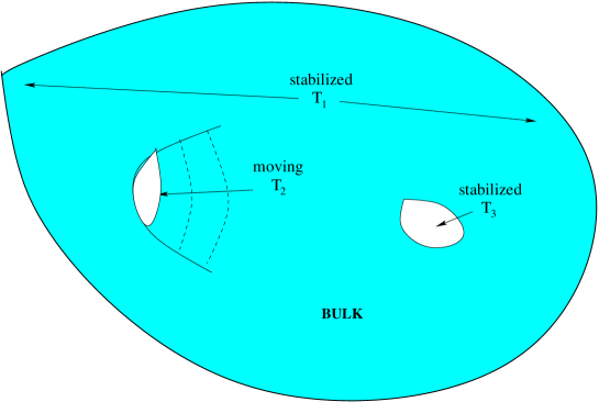
Figure 1: Schematic illustration of the ingredients in Kähler moduli inflation. The four-cycles of the CY are the Kähler moduli $T_{i}$ which govern the sizes of different holes in the manifold. We assume $T_{3}$ and the overall scale $T_{1}$ are already stabilized, while the last modulus to stabilize, $T_{2}$, drives inflation while settling down to its minimum. The imaginary parts of $T_{i}$ have to be left to the imagination. The outer $3+1$ observable dimensions are also not shown.

In this picture, the theory prior would itself be a Bayesian product of a number of conditional probabilities: (1) of manifold configuration defining the moduli; (2) of parameters defining the effective potential and the non-canonical kinetic energy of the moduli, given the manifold structure; (3) of the initial conditions for the moduli and their field momenta given the potentials. The latter will depend upon exactly how the “rain down” from higher energies occurs to populate $T_{2}$ initial conditions. An effective complication occurs because of the so-called eternal inflation regime, when the stochastic kicks that the inflaton feels in an e-folding can be as large as the classical drift. This $T_{2}$-model is in fact another example of stringy inflation with self-reproduction. (See [2] for another case.) If other higher-energy moduli are frozen out, most inflationary trajectories would emerge from this quantum domain. However we expect other quantum domains for the higher-energy moduli to also feed the $T_{2}$ initial conditions, so we treat these as arbitrary.

The Kähler moduli are flat directions at the stringy tree level. The reason this picture works is that the leading non-perturbative (instanton) and perturbative ($\alpha^{\prime}$) corrections introduce only an exponentially flat dependence on the Kähler moduli, avoiding the $\eta$-problem. Conlon and Quevedo [9] focused on the real part of $T_{2}$ as the inflaton and showed that slow-roll inflation with enough e-foldings was possible. A modification [14] of the model considered inflation in a new $\mathcal{V}$ direction but with a negative result.

The fields $T_{i}$ are complex, $T_{i}=\tau_{i}+i\theta_{i}$. In this paper we extend the model of [9] to include the axionic direction $\theta_{2}$. There is essentially only one trajectory if $\theta_{2}$ is forced to be fixed at its trough, as in [9]. The terrain in the scalar potential $V(\tau_{2},\theta_{2})$ has hills and valleys in the $\theta_{2}$ direction which results in an ensemble of trajectories depending upon the initial values of $\tau_{2},\theta_{2}$. The field momenta may also be arbitrary but their values quickly relax to attractor values. The paper [15] considered inflation only along the $\theta$ direction while the dynamics in the $\tau$ direction were artificially frozen. We find motion in $\tau$ always accompanies motion in $\theta$.

In Kähler moduli models, there is an issue of higher order perturbative corrections. Even a tiny quadratic term would break the exponential flatness of the inflaton potential and could make the $\eta$-problem reappear. However, the higher order terms which depend on the inflaton only through the overall volume $\mathcal{V}$ of the Calabi-Yau manifold will not introduce any mass terms for the inflaton. Although these corrections may give rise to a mass term for the inflaton, it might have a limited effect on the crucial last sixty e-folds.

In § 2 we describe the model in the context of type IIB string theory. In § 3 we address whether higher (sub-leading) perturbative corrections introduce a dangerous mass term for the inflaton. In § 4 we discuss the effective potential for the volume, Kähler moduli and axion fields, showing with 3 moduli that stabilization of two of them can be sustained even as the inflaton $T_{2}$ evolves. Therefore in § 5 we restrict ourselves to $V(\tau_{2},\theta_{2})$ with the other moduli stabilized at their minima. § 6 explores inflationary trajectories generated with that potential, for various choices of potential parameters and initial conditions. In § 7 we investigate the diffusion/drift boundary and the possibility of self-reproduction. In § 8 we summarize our results and outline issues requiring further consideration, such as the complication in power spectra computation that follows from the $\tau_{2},\theta_{2}$ freedom.

2 The Type IIB String Theory Model

Our inflationary model is based on the “large-volume” moduli stabilization mechanism of [11, 12, 13]. This mechanism relies upon the fixing of the Kähler moduli in IIB flux compactifications on Calabi-Yau (CY) manifolds $M$ by non-perturbative as well as perturbative effects. As argued in [11, 12, 13], a minimum of the moduli potential in the effective $4d$ theory exists for a large class of models. The only restriction is that there should be more complex structure moduli in the compactification than Kähler moduli, i.e. $h^{1,2}>h^{1,1}>1$, where $h^{1,2},h^{1,1}$ are the Hodge numbers of the CY. (The number of complex structure moduli is $h^{1,2}$ and the number of Kähler moduli is $h^{1,1}$. Other Hodge numbers are fixed for a CY threefold.) The “large-volume” moduli stabilization mechanism is an alternative to the KKLT one, although it shares some features with KKLT. The purpose of this section is to briefly explain the model of [11, 12, 13].

An effective $4d$ $\mathcal{N}=1$ supergravity is completely specified by a Kähler potential, superpotential and gauge kinetic function. In the scalar field sector of the theory the action is

$$S_{\mathcal{N}=1}=\int d^{4}x\sqrt{-g}\left[\frac{M_{P}^{2}}{2}\mathcal{R}-\mathcal{K}_{,i\bar{j}}D_{\mu}\phi^{i}D^{\mu}\bar{\phi}^{j}-V(\phi,\bar{\phi})\right],$$ (2)

where

$$V(\phi,\bar{\phi})=e^{\mathcal{K}/M_{P}^{2}}\left(\mathcal{K}^{i\bar{j}}D_{i}\hat{W}D_{\bar{j}}\bar{\hat{W}}-\frac{3}{M_{P}^{2}}\hat{W}\bar{\hat{W}}\right)+\textrm{ D-terms}.$$ (3)

Here $\mathcal{K}$ and $\hat{W}$ are the Kähler potential and the superpotential respectively, $M_{P}$ is the reduced Planck mass eq.(1), and $\phi^{i}$ represent all scalar moduli. (We closely follow the notations of [13] and keep $M_{P}$ and other numerical factors explicit.)

The $\alpha^{\prime 3}$-corrected Kähler potential [16] is

$$\frac{\mathcal{K}}{M_{P}^{2}}=-2\ln\left(\mathcal{V}+\frac{\xi g_{s}^{\frac{3}{2}}}{2e^{\frac{3\phi}{2}}}\right)-\ln(S+\bar{S})-\ln\left(-i\int_{M}\Omega\wedge\bar{\Omega}\right).$$ (4)

Here $\mathcal{V}$ is the volume of the CY manifold $M$ in units of the string length $l_{s}=2\pi\sqrt{\alpha^{\prime}}$, $\mathcal{V}=\mathcal{V}_{s}l_{s}^{6}$ and we set $\alpha^{\prime}=1$. The second term in the logarithm represents the $\alpha^{\prime}$-corrections with $\xi=-\frac{\zeta(3)\chi(M)}{2(2\pi)^{3}}$ proportional to the Euler characteristic $\chi(M)$ of the manifold $M$. $S=-iC_{0}+e^{-\phi}$ is the IIB axio-dilaton with $\phi$ the dilaton component and $C_{0}$ the Ramond-Ramond 0-form. $\Omega$ is the holomorphic 3-form of $M$. The superpotential depends explicitly upon the Kähler moduli $T_{i}$ when non-perturbative corrections are included

$$\hat{W}=\frac{g_{s}^{\frac{3}{2}}M_{P}^{3}}{\sqrt{4\pi}}\left(W_{0}+\sum_{i=1}^{h^{1,1}}A_{i}e^{-a_{i}T_{i}}\right),\quad W_{0}=\frac{1}{l_{s}^{2}}\int_{M}G_{3}\wedge\Omega.$$ (5)

Here, $W_{0}$ is the tree level flux-induced superpotential which is related to the IIB flux 3-form $G_{3}=F_{3}-iSH_{3}$ as shown. The exponential terms $A_{i}e^{-a_{i}T_{i}}$ are from non-perturbative (instanton) effects. (For simplicity, we ignore higher instanton corrections. This should be valid as long as we restrict ourselves to $a_{i}\tau_{i}\gg 1$, which we do.) The Kähler moduli are complex,

$$T_{i}=\tau_{i}+i\theta_{i}\,,$$ (6)

with $\tau_{i}$ the 4-cycle volume and $\theta_{i}$ its axionic partner, arising from the Ramond-Ramond 4-form $C_{4}$. The $A_{i}$ encode threshold corrections. In general they are functions of the complex structure moduli and are independent of the Kähler moduli. This follows from the requirement that $W$ is a holomorphic function of complex scalar fields and therefore can depend on $\tau_{i}$ only via the combination $T_{i}=\tau_{i}+i\theta_{i}$. On the other hand, $W$ should respect the axion shift symmetry $\theta_{i}\to\theta_{i}+\frac{2\pi}{a_{i}}$ and thus cannot be a polynomial function of $T_{i}$. (See [17] for discussion.)

The critical parameters $a_{i}$ in the potential are constants which depend upon the specific nature of the dominant non-perturbative mechanism. For example, $a_{i}=\frac{2\pi}{g_{s}}$ for Euclidean D3-brane instantons and $a_{i}=\frac{2\pi}{g_{s}N}$ for the gaugino condensate on the D7 brane world-volume. We vary them freely in our exploration of trajectories in different potentials.

It is known that both the dilaton and the complex structure moduli can be stabilized in a model with a tree level superpotential $W_{0}$ induced by generic supersymmetric fluxes (see e.g. [18]) and the lowest-order (i.e. $\xi=0$) Kähler potential, whereas the Kähler moduli are left undetermined in this procedure (hence are “no scale” models). Including both leading perturbative and non-perturbative corrections and integrating out the dilaton and the complex structure moduli, one obtains a potential for the Kähler moduli which in general has two types of minima. The first type is the KKLT minima [1] which requires significant fine tuning of $W_{0}$ ($\sim 10^{-4}$) for their existence. As pointed out in [13], the KKLT approach has a few shortcoming, among which are the limited range of validity of the KKLT effective action (due to $\alpha^{\prime}$ corrections) and the fact that either the dilaton or some of the complex structure moduli typically become tachyonic at the minimum for the Kähler modulus. (We note, however, that [19] argued that a consistent KKLT-type model with all moduli properly stabilized can be found.) The second type is the “large-volume” AdS minima studied in [11, 12, 13]. These minima exist in a broad class of models and at arbitrary values of parameters. An important characteristic feature of these models is that the stabilized volume of the internal manifold is exponentially large, $\mathcal{V}_{min}\sim\exp{(a\tau_{min})}$, and can be $\mathcal{O}(10^{5}-10^{20})$ in string units. (Here $\tau_{min}$ is the value of $\tau$ at its minimum.) The relation between the Planck scale and string scale is

$$M_{P}^{2}=\frac{4\pi\mathcal{V}_{min}}{g_{s}^{2}}m_{s}^{2}\,,$$ (7)

where $\mathcal{V}_{min}$ is the volume in string units at the minimum of the potential. Thus these models can have $m_{s}$ in the range between the GUT and TeV scale. In these models one can compute the spectrum of low-energy particles and soft supersymmetry breaking terms after stabilizing all moduli, which makes them especially attractive phenomenologically (see [13, 20]).

Conlon and Quevedo [9] studied inflation in these models and showed that there is at least one natural inflationary direction in the Kähler moduli space. The non-perturbative corrections in the superpotential eq.(5) depend exponentially on the Kähler moduli $T_{i}$, and realize by eq.(3) exponentially flat inflationary potentials, the first time this has arisen from string theory. As mentioned in § 1, higher (sub-leading) $\alpha^{\prime}$ and string loop corrections could, in principle, introduce a small polynomial dependence on the $T_{i}$ which would beat exponential flatness at large values of the $T_{i}$. Although the exact form of these corrections is not known, we assume in this paper that they are not important for the values of the $T_{i}$ during the last stage of inflation (see § 3).

After stabilizing the dilaton and the complex structure moduli we can identify the string coupling as $g_{s}=e^{\phi}$, so the Kähler potential (4) takes the simple form

$$\frac{\mathcal{K}}{M_{P}^{2}}=-2\ln\left(\mathcal{V}+\frac{\xi}{2}\right)+\ln g_{s}+\mathcal{K}_{cs}\,,$$ (8)

where $\mathcal{K}_{cs}$ is a constant. Using this formula together with equations (3), (5), and (11), one can compute the scalar potential. In our subsequent analysis, we shall absorb the constant factor $e^{\mathcal{K}_{cs}}$ into the parameters $W_{0}$ and $A_{i}$.

The volume of the internal CY manifold $M$ can be expressed in terms of the 2-cycle moduli $t^{i},\,i=1,...,n=h^{1,1}$:

$$\mathcal{V}=\frac{1}{6}\kappa_{ijk}t^{i}t^{j}t^{k}\,,$$ (9)

where $\kappa_{ijk}$ is the triple intersection form of $M$. The 4-cycle moduli $\tau_{i}$ are related to the $t^{i}$ by

$$\tau_{i}=\frac{\partial}{\partial t^{i}}\mathcal{V}=\frac{1}{2}\kappa_{ijk}t^{j}t^{k}\,,$$ (10)

which gives $\mathcal{V}$ an implicit dependence on the $\tau_{i}$, and thus $\mathcal{K}$ through eq.(8). It is known [21] that for a CY manifold the matrix $\frac{\partial^{2}\mathcal{V}}{\partial t^{i}\partial t^{j}}$ has signature $(1,h^{1,1}-1)$, with one positive eigenvalue and $h^{1,1}-1$ negative eigenvalues. Since $\tau_{i}=\tau_{i}(t^{j})$ is just a change of variables, the matrix $\frac{\partial^{2}\mathcal{V}}{\partial\tau_{i}\partial\tau_{j}}$ also has signature $(1,h^{1,1}-1)$. In the case where each of the 4-cycles has a non-vanishing triple intersection only with itself, the matrix $\frac{\partial^{2}\mathcal{V}}{\partial\tau_{i}\partial\tau_{j}}$ is diagonal and its signature is manifest. The volume in this case takes a particularly simple form in terms of the $\tau_{i}$:

$$\mathcal{V}=\alpha\left(\tau_{1}^{3/2}-\sum_{i=2}^{n}\lambda_{i}\tau_{i}^{3/2}\right)\,.$$ (11)

Here $\alpha$ and $\lambda_{i}$ are positive constants depending on the particular model. This formula suggests a “Swiss-cheese” picture of a CY, in which $\tau_{1}$ describes the 4-cycle of maximal size and $\tau_{2},\ldots,\tau_{n}$ the blow-up cycles. The modulus $\tau_{1}$ controls the overall scale of the CY and can take an arbitrarily large value, whereas $\tau_{2},\ldots,\tau_{n}$ describe the holes in the CY and cannot be larger than the overall size of the manifold. As argued in [12, 13], for generic values of the parameters $W_{0}$, $A_{i}$, $a_{i}$ one finds that $\tau_{1}\gg\tau_{i}$ and $\mathcal{V}\gg 1$ at the minimum of the effective potential. In other words, the sizes of the holes are generically much smaller than the overall size of the CY.

The role of the inflaton in the model of [9] is the last modulus among the $\tau_{i}$, $i=2,...,n$, to attain its minimum. As noted by [9], the simplified form of the volume eq.(11) is not really necessary to have inflation. For our analysis to be correct, it would be enough to consider a model with at least one Kähler modulus whose only non-zero triple intersection is with itself, i.e.,

$$\mathcal{V}=\alpha(...-\lambda_{i}\tau_{i}^{3/2})\,,$$ (12)

and which has its own non-perturbative term in the superpotential eq.(5).

3 Perturbative Corrections

There are several types of perturbative corrections that could modify the classical potential on the Kähler moduli space: those related to higher string modes, or $\alpha^{\prime}$-corrections, coming from the higher derivative terms in both bulk and source (brane) effective actions; and string loop, or $g_{s}$-corrections, coming from closed and open string loop diagrams.

As we mentioned before, $\alpha^{\prime}$-corrections are an important ingredient of the “large volume” compactification models of [11, 12, 13]. They are necessary for the existence of the large volume minimum of the effective potential in the models with Kähler moduli “lifted” by instanton terms in the superpotential. The leading $\alpha^{\prime}$-corrections to the potential arise from the higher derivative terms in the ten dimensional IIB action at the order $\sim\alpha^{\prime 3}$,

$$S_{IIB}=-\frac{1}{2\kappa_{10}^{2}}\,\int d^{10}x\sqrt{-g^{(10)}}e^{-2\phi}[R+4(\partial\phi)^{2}+\alpha^{\prime 3}\frac{\zeta(3)}{3\cdot 2^{11}}\,J_{0}-\alpha^{\prime 3}\frac{(2\pi)^{3}\zeta(3)}{4}\,Q+...]\,,$$ (13)

where $J_{0}\sim(R^{MN}{}_{PQ})^{4}$ and $Q$ is a generalization of the six-dimensional Euler integrand,

$$\int_{M}d^{6}x\sqrt{g}Q=\chi\,.$$ (14)

Performing a compactification of (13) on a CY threefold, one finds $\alpha^{\prime}$-corrections to the metric on the Kähler moduli space, which can be described by the $\xi$-term in the Kähler potential (4) (see [23, 16]). We will see later that this correction introduces a positive term $\sim\xi W_{0}^{2}/\mathcal{V}^{3}$ into the potential. As discussed in [13], further higher derivative bulk corrections at $\mathcal{O}(\alpha^{\prime 4})$ and above are sub-leading to the $1/\mathcal{V}^{3}$ term and therefore suppressed. (Note that in the models we are dealing with, there is effectively one more expansion parameter, $1/\mathcal{V}$, due to the large value of the stabilized $\mathcal{V}$.) Also, $\alpha^{\prime}$-corrections from the D3/D7 brane actions depend on 4d space-time curvatures and, therefore, do not contribute to the potential. String loop corrections to the Kähler potential come from the Klein bottle, annulus and Möbius strip diagrams computed in [24] for the models compactified on the orientifolds of tori. The Kähler potential including both leading $\alpha^{\prime}$ and loop corrections can be schematically written as [24]

$$K=-2\ln{\mathcal{V}}-{\xi\over\mathcal{V}}+{f_{1}\over\mathcal{V}^{2/3}}+{f_{2}\over\mathcal{V}^{4/3}}+...\,.$$ (15)

(We have dropped terms depending only on the brane and complex structure moduli.) Here $f_{1}$ and $f_{2}$ are functions of the moduli whose forms are unknown for a generic CY manifold. If they depend upon the inflaton $\tau_{i}$ polynomially, a mass term will arise for $\tau_{i}$ with the possibility of an $\eta$-problem. Further study is needed to decide. Note that, although the exact form of higher (sub-leading) corrections is unknown, any correction which introduces dependence on $\tau_{i}$ only via $\mathcal{V}$ will not generate any new mass terms for $\tau_{i}$.

As well as $\tau$-corrections there are possible $\theta$-corrections. Non-perturbative effects modify the superpotential by breaking the shift symmetry, making it discrete. As noted we do include these. Although leading perturbative terms leave the Kähler potential $\theta$-independent, subleading corrections can lead to $\theta$-dependent modifications, which we ignore here.

In this paper, we assume that the higher corrections, though possibly destroying slow roll at large values of the inflaton, are not important during the last stage of inflation.

4 Effective Potential and Volume Stabilization

In this Section, we sketch the derivation of the effective field theory potential starting from equations (3,5,8). We choose $T_{2}$ to be the inflaton field and study its dynamics in the 4-dimensional effective theory. We first have to ensure that the volume modulus $\mathcal{V}$ and other Kähler moduli are trapped in their minima and remain constant or almost constant during inflation. For this we have to focus on the effective potential of all relevant fields.

Given the Kähler potential and the superpotential, it is straightforward but tedious to compute the scalar potential as a function of the fields $T_{i}$. To make all computations we modified the SuperCosmology Mathematica package [25] which originally was designed for real scalar fields to manipulate complex fields.

The Kähler potential (8) gives rise to the Kähler metric $K_{i\bar{j}}=\frac{\partial^{2}K}{\partial T^{i}\partial\bar{T}^{\bar{j}}}$, with

$$K_{1\bar{1}}=\frac{3\alpha(4\mathcal{V}-\xi+6\alpha(\sum_{k=2}^{n}\lambda_{k}\tau_{k}^{3/2}))}{4(2\mathcal{V}+\xi)^{2}(\frac{\mathcal{V}}{\alpha}+\sum_{k=2}^{n}\lambda_{k}\tau_{k}^{3/2})^{1/3}}\ , K_{i\bar{j}}=\frac{9\alpha^{2}\lambda_{i}\lambda_{j}\sqrt{\tau_{i}\tau_{j}}}{2(2\mathcal{V}+\xi)^{2}}\ ,$$

$$K_{1\bar{j}}=-\frac{9\lambda_{j}\sqrt{\tau_{j}}(\alpha^{5}(\mathcal{V}+\alpha\sum_{k=2}^{n}\lambda_{k}\tau_{k}^{3/2}))^{1/3}}{2(2\mathcal{V}+\xi)^{2}}\ , K_{i\bar{i}}=\frac{3\alpha\lambda_{i}(2\mathcal{V}+\xi+6\alpha\sum_{k=2}^{n}\lambda_{k}\tau_{k}^{3/2})}{4(2\mathcal{V}+\xi)^{2}\sqrt{\tau_{i}}}\ .\qquad$$ (16)

This can be inverted to give

$$K^{1\bar{1}}=\frac{4(2\mathcal{V}+\xi)(\mathcal{V}+\alpha\sum_{k=2}^{n}\lambda_{k}\tau_{k}^{3/2})^{1/3}(2\mathcal{V}+\xi+6\alpha\sum_{k=2}^{n}\lambda_{k}\tau_{k}^{3/2})}{3\alpha^{4/3}(4\mathcal{V}-\xi)}\ ,K^{i\bar{j}}=\frac{8(2\mathcal{V}+\xi)\tau_{i}\tau_{j}}{4\mathcal{V}-\xi}\ ,$$

$$K^{1\bar{j}}=\frac{8(2\mathcal{V}+\xi)\tau_{j}(\frac{\mathcal{V}}{\alpha}+\sum_{k=2}^{n}\lambda_{k}\tau_{k}^{3/2})^{2/3}}{4\mathcal{V}-\xi}\ ,K^{i\bar{i}}=\frac{4(2\mathcal{V}+\xi)\sqrt{\tau_{i}}(4\mathcal{V}-\xi+6\alpha\sum_{k=2}^{n}\lambda_{k}\tau_{k}^{3/2})}{3\alpha(4\mathcal{V}-\xi)\lambda_{2}}\ .$$ (17)

This is the full expression for an arbitrary number of Kähler moduli $T_{i}$. The entries of the metric contain terms of different orders in the inverse volume. If we were to keep only the lowest order terms $\mathrel{\hbox to0.0pt{\lower 4.0pt\hbox{\hskip 1.0pt$\sim$}\hss}\raise 1.0pt\hbox{$>$}}\mathcal{O}({1\over\mathcal{V}^{3}})$, the shape of the trajectories we determine in the following sections and our conclusions would remain practically unchanged. That is, we are working with higher precision than necessary. Note that the kinetic terms for $\tau$ and $\theta$ are identical, appearing as $K_{2\bar{2}}(\partial\tau\partial\tau+\partial\theta\partial\theta)$ in the Lagrangian.

The resulting potential is

$$V(T_{1},...,T_{n}) = \frac{12W_{0}^{2}\xi}{(4\mathcal{V}-\xi)(2\mathcal{V}+\xi)^{2}}+\sum_{i=2}^{n}\frac{12e^{-2a_{i}\tau_{i}}\xi A_{i}^{2}}{(4\mathcal{V}-\xi)(2\mathcal{V}+\xi)^{2}}+\frac{16(a_{i}A_{i})^{2}\sqrt{\tau_{i}}e^{-2a_{i}\tau_{i}}}{3\alpha\lambda_{2}(2\mathcal{V}+\xi)}$$

$${}+\frac{32e^{-2a_{i}\tau_{i}}a_{i}A_{i}^{2}\tau_{i}(1+a_{i}\tau_{i})}{(4\mathcal{V}-\xi)(2\mathcal{V}+\xi)}+\frac{8W_{0}A_{i}e^{-a_{i}\tau_{i}}\cos(a_{i}\theta_{i})}{(4\mathcal{V}-\xi)(2\mathcal{V}+\xi)}\left(\frac{3\xi}{(2\mathcal{V}+\xi)}+4a_{i}\tau_{i}\right)$$

$${}+\sum_{{i,j=2\atop i<j}}^{n}\frac{A_{i}A_{j}\cos(a_{i}\theta_{i}-a_{j}\theta_{j})}{(4\mathcal{V}-\xi)(2\mathcal{V}+\xi)^{2}}\,e^{-(a_{i}\tau_{i}+a_{j}\tau_{j})}\left[32(2\mathcal{V}+\xi)(a_{i}\tau_{i}+a_{j}\tau_{j}\right.$$

$${}\left.+2a_{i}a_{j}\tau_{i}\tau_{j})+24\xi\right]+V_{\mathrm{uplift}}\ .$$

We have to add here the uplift term $V_{\mathrm{uplift}}$ to get a Minkowski or tiny dS minimum. Uplifting is not just a feature needed in string theory models. For example, uplifting is done in QFT to tune the constant part of the scalar field potential to zero. At least in string theory there are tools for uplifting, whereas in QFT it is a pure tuning (see, e.g., [1, 26] and references therein). We will adopt the form

$$V_{\mathrm{uplift}}=\frac{\beta}{\mathcal{V}^{2}}\,,$$ (19)

with $\beta$ to be adjusted.

We now discuss the stabilization of all moduli $T_{i}$ plus the volume modulus. For this we have to find the global minimum of the potential eq.(4), which we do numerically. However, it is instructive to give analytic estimations. Following [12, 13], we study an asymptotic form of eq.(4) in the region where both $\mathcal{V}\sim\exp{(a_{i}\tau_{i})}$, $i=2,...,n$, and $\mathcal{V}\gg 1$. The potential is then a series of inverse powers of $\mathcal{V}$. Keeping the terms up to the order $\mathcal{O}(\frac{1}{\mathcal{V}^{3}})$ we obtain

$$V=\frac{1}{\mathcal{V}}\sum_{i=2}^{n}\frac{8(a_{i}A_{i})^{2}\sqrt{\tau_{i}}}{\lambda_{i}\alpha}e^{-2a_{i}\tau_{i}}+\frac{4}{\mathcal{V}^{2}}\sum_{i=2}^{n}a_{i}A_{i}W_{0}\tau_{i}e^{-a_{i}\tau_{i}}\cos(a_{i}\theta_{i})+\frac{3\xi W_{0}^{2}}{4\mathcal{V}^{3}}+\frac{\beta}{\mathcal{V}^{2}}\ .$$ (20)

The cross terms for different $\tau_{i}$ do not appear in this asymptotic form, as they would be of order $1/\mathcal{V}^{5}$. Requiring $\frac{\partial V}{\partial\tau_{i}}=0$ and $\cos(a_{i}\theta_{i})=-1$ at the minimum of the potential eq.(20), we get

$$\mathcal{V}_{min}\sim\frac{W_{0}\lambda_{2}}{a_{2}A_{2}}\sqrt{\tau_{2,min}}e^{a_{2}\tau_{2,min}}\sim\frac{W_{0}\lambda_{3}}{a_{3}A_{3}}\sqrt{\tau_{3,min}}e^{a_{3}\tau_{3,min}}\sim...\sim\frac{W_{0}\lambda_{i}}{a_{n}A_{n}}\sqrt{\tau_{n,min}}e^{a_{n}\tau_{n,min}}\ ,$$ (21)

where $\tau_{i,min}$ are the values of the moduli at the global minimum. The expression (20) has the structure

$$V=\frac{C_{1}}{\mathcal{V}}+\frac{C_{2}}{\mathcal{V}^{2}}+\frac{C_{3}}{\mathcal{V}^{3}}\ ,$$ (22)

where the coefficients $C_{1},C_{2},C_{3}$ are functions of $\tau_{i}$ and $\theta_{i}$. $C_{1}$ and $C_{3}$ are positive but $C_{2}$ can be of either sign. However, the potential for the volume $\mathcal{V}$ has a minimum only if $C_{2}<0$, which is achieved for $\cos(a_{i}\theta_{i})<0$; otherwise $V(\mathcal{V})$ would have a runaway character. Also if all $\tau_{i}$ are very large so that $e^{-a_{i}\tau_{i}}\to 0$, then $C_{2}\to 0$ and $\mathcal{V}$ cannot be stabilized. Therefore to keep $C_{2}$ non-zero and negative we have to require that some of the $i>2$ Kähler moduli $\tau_{i}$ and their axionic partners are trapped in the minimum. For simplicity we assume all but $T_{2}$ are already trapped in the minimum.

It is important to recognize that trapping all moduli but one in the minimum cannot be achieved with only two Kähler moduli $\tau_{1}$ and $\tau_{2}$, because $\tau_{1}$ effectively corresponds to the volume, and $\tau_{2}$ is the inflaton which is to be placed out of the minimum. The Fig. 2 shows the potential as a function of $\tau_{1}$ and $\tau_{2}$ for the two-Kähler model. One can see from this plot that a trajectory starting from an initial value for $\tau_{2}$ larger than a critical value will have runaway behavior in the $\tau_{1}$ (volume) direction. Thus, as shown by [9], one has to consider a model with three or more Kähler moduli.

(a) (b)

Figure 2: (a) The potential surface $V(\tau_{1},\tau_{2})$ in a two-Kähler model, with the axionic components $\theta_{1}$ and $\theta_{2}$ fixed at their minima. (b) shows the related contour plot of the volume $\mathcal{V}$ against $\tau_{2}$. Although it may be possible to find a local (very shallow) minimum for the volume in this model (marked by a star), the generic situation is that both $\tau_{1}$ and $\tau_{2}$ will be dynamical, and indeed, the evolving $\tau_{2}$ could force $\tau_{1}$ out of a local minimum, thereby destabilizing what may have once been stabilized. For this reason, we have focused on models with three or more Kähler moduli, with all but one mutually enforcing their respective stabilizations, and in particular that of the volume. This large volume multi-Kähler approach to stabilization differs from the KKLT stabilization mechanism.

By contrast, the “better racetrack” inflationary model based on the KKLT stabilization is achieved with just two Kähler moduli [3]. However, in our class of models with three and more Kähler moduli we have more flexibility in parameter space in achieving both stabilization and inflation. Another aspect of the work in this paper is that a “large volume” analog of the “better racetrack” model may arise.

We have learned that to be fully general we would allow all other moduli including the volume $\mathcal{V}$ to be dynamical. This will lead to even richer possibilities than those explored here, where we only let $T_{2}$ evolve, and assume that varying it does not alter the values of the other moduli which we pin at the global minimum. To demonstrate this is viable, we need to show the contribution of $T_{2}$ to the position of the minimum is negligible. Following [9], we set all $\tau_{i}$, $i=2,...,n$, and their axions $\theta_{i}$ to their minima and use equations (20) and (21) to obtain the potential for $\mathcal{V}$:

$$V(\mathcal{V})=-\frac{3W_{0}^{2}}{2\mathcal{V}^{3}}\left(\alpha\sum_{i=2}^{n}\left[\frac{\lambda_{i}}{a_{i}^{3/2}}\right](\ln\mathcal{V})^{3/2}-\frac{\xi}{2}\right)+\frac{\beta}{\mathcal{V}^{2}}\,.$$ (23)

As one can see from eq.(20), the contribution of $T_{2}$ to the potential is maximal (by absolute value) when $\tau_{2}$ and $\theta_{2}$ are at their minimum, and vanishes as $\tau_{2}\to+\infty$. This gives a simple criterion for whether the minimum for the volume $\mathcal{V}$ remains stable during the evolution of $T_{2}$: the functional form of the potential for $\mathcal{V}$ (23) is insensitive to $T_{2}$ provided [9]:

$$\sum_{i=3}^{n}\frac{\lambda_{i}}{a_{i}^{3/2}}\gg\frac{\lambda_{2}}{a_{2}^{3/2}}\ .$$ (24)

For a large enough number of Kähler moduli this condition is automatically satisfied for generic values of $a_{i}$ and $\lambda_{i}$. We conclude that with many Kähler moduli the volume does not change during the evolution of the inflaton $T_{2}$ because the other $T_{i}$ stay at their minimum and keep the volume stable.

Consider a toy model with three Kähler moduli in which $T_{2}$ is the inflaton and $T_{3}$ stays at its own minimum to provide an unvarying minimum for $\mathcal{V}$. We choose parameters as in set 1 in Table 1 (which will be explained in detail below in Sec. 5), and also let $a_{3}=2\pi/300$, $A_{3}=1/200$, and $\lambda_{3}=10$. Eq.(24) is strongly satisfied, ${\frac{\lambda_{2}}{a_{2}^{3/2}}}\Big{/}{\frac{\lambda_{3}}{a_{3}^{3/2}}}=10^{-4}$, under this choice of parameters. Therefore we can drop the $\tau_{2},\theta_{2}$-dependent terms in the potential (20) and use it as a function of the two fields $\mathcal{V}$ and $\tau_{3}$ to find their values at the minimum (after setting also $\theta_{3}=\pi/a_{3}$ to its minimum). The minimization procedure should also allow one to adjust the uplift parameter $\beta$ in a way that the potential vanishes at its global minimum. With our choice of parameters we found the minimum numerically to be at $\tau_{3}=49$ and $\mathcal{V}=10^{6}$ with $\beta=8.5\times 10^{-6}$, as shown in Fig. 3.

(a) (b)

Figure 3: One dimensional sections of the uplifted potential for parameter set 1. We perform a proper uplift procedure by explicitly introducing the additional field $\tau_{3}$ which is responsible for stabilizing the volume during inflation. The parameters for $\tau_{3}$ are chosen in such a way that the stability condition is fulfilled and at the same time we recover the desired value of $\mathcal{V}_{min}\approx 10^{6}$. The minimum in $\tau_{3}$ direction is clearly visible at $\tau_{3,min}\approx 49$.

5 Inflaton Potential

We now take all moduli $T_{i}$, $i>3$, and the volume $\mathcal{V}$ (hence $T_{1}$) to be fixed at their minima, but let $T_{2}$ vary, since it is our inflaton. For simplicity in the subsequent sections we drop the explicit subscript, setting $T_{2}=\tau+i\theta$. The scalar potential $V(\tau,\theta)$ is obtained from eq.(4) with the other Kähler moduli stabilized:

$$V(\tau,\theta)=\frac{12W_{0}^{2}\xi}{(4\mathcal{V}_{m}-\xi)(2\mathcal{V}_{m}+\xi)^{2}}+\frac{D_{1}+12e^{-2a_{2}\tau}\xi A_{2}^{2}}{(4\mathcal{V}_{m}-\xi)(2\mathcal{V}_{m}+\xi)^{2}}+\frac{D_{2}+\frac{16(a_{2}A_{2})^{2}}{3\alpha\lambda_{2}}\sqrt{\tau}e^{-2a_{2}\tau}}{(2\mathcal{V}_{m}+\xi)}$$ (25)

$$+\frac{D_{3}+32e^{-2a_{2}\tau}a_{2}A_{2}^{2}\tau(1+a_{2}\tau)}{(4\mathcal{V}_{m}-\xi)(2\mathcal{V}_{m}+\xi)}+\frac{D_{4}+8W_{0}A_{2}e^{-a_{2}\tau}\cos(a_{2}\theta)}{(4\mathcal{V}_{m}-\xi)(2\mathcal{V}_{m}+\xi)}\left(\frac{3\xi}{(2\mathcal{V}_{m}+\xi)}+4a_{2}\tau\right)+\frac{\beta}{\mathcal{V}_{m}^{2}}\ .$$

Here the terms $D_{1},...,D_{4}$ contain contributions from the stabilized Kähler moduli other than the inflaton. We dropped cross terms between $\tau$ and other $\tau_{i}$, $i>3$, since these are suppressed by inverse powers of $\mathcal{V}_{m}$. We can trust eq.(25) only up to the order $1/\mathcal{V}^{3}$; at higher orders in $1/\mathcal{V}$, higher perturbative corrections to the Kähler potential eq.(15) start contributing. Explicitly expanding to order $1/\mathcal{V}^{3}$ yields the simpler expression

$$V(\tau,\theta)=\frac{8(a_{2}A_{2})^{2}\sqrt{\tau}e^{-2a_{2}\tau}}{3\alpha\lambda_{2}\mathcal{V}_{m}}-\frac{4W_{0}a_{2}A_{2}\tau e^{-a_{2}\tau}\cos{(a_{2}\theta)}}{\mathcal{V}_{m}^{2}}+\Delta V\ ,$$ (26)

where

$$\Delta V=\frac{3W_{0}^{2}\xi}{4\mathcal{V}_{m}^{3}}+\frac{D_{2}}{\mathcal{V}_{m}}+\frac{\beta-D_{4}}{\mathcal{V}_{m}^{2}}$$ (27)

is a constant term, since $\mathcal{V}$ and $\tau_{i}$, $i>3$ are all stabilized at the minimum, and $D_{2}$, $D_{4}$ depend only on these $\tau_{i}$.

Parameter	$W_{0}$	$a_{2}$	$A_{2}$	$\lambda_{2}$	$\alpha$	$\xi$	$g_{s}$	$\mathcal{V}$	$\Delta\varphi/M_{p}$
Parameter set 1	$300$	$2\pi/3$	$0.1$	$1$	$1/9\sqrt{2}$	$0.5$	$1/10$	$10^{6}$	$2\times 10^{-3}$
Parameter set 2	$6\times 10^{4}$	$2\pi/30$	$0.1$	$1$	$1/9\sqrt{2}$	$0.5$	$1/10$	$10^{8}$	$1\times 10^{-3}$
Parameter set 3	$4\times 10^{5}$	$\pi/100$	$1$	$1$	$1/9\sqrt{2}$	$0.5$	$1/10$	$10^{9}$	$1.4\times 10^{-3}$
Parameter set 4	$200$	$\pi$	$0.1$	$1$	$1/9\sqrt{2}$	$0.5$	$1/10$	$10^{6}$	$1.5\times 10^{-3}$
Parameter set 5	$100$	$2\pi/3$	$0.1$	$1$	$1/9\sqrt{2}$	$0.5$	$1/10$	$10^{6}$	$1.9\times 10^{-3}$
Parameter set 6	$75$	$2\pi/6$	$1$	$1$	$1/9\sqrt{2}$	$0.5$	$1/10$	$10^{8}$	$4\times 10^{-4}$

Table 1: Sample parameter sets for the $T_{2}$ inflation model. Sets 1 to 4 define models in which the primordial power spectra of perturbations are approximately compatible with observations, whereas sets 5 and 6 do not. There are approximate scaling relations which map one set of parameters without changing the power spectrum (see explanation in the text regarding $W_{0}$). The value of $W_{0}$ in sets 2 and 3 is so high that corrections to the potential seem likely to appear. We note however that these large values can be reduced using the scaling transformation, but the undesirable cost is that $\tau$ can drop below the string scale or $a_{2}$ can become too large. The last column shows approximate values for the variation of the canonically-normalized inflaton eq.(29) over the observable e-fold range, appropriately small cf. the Planck scale.

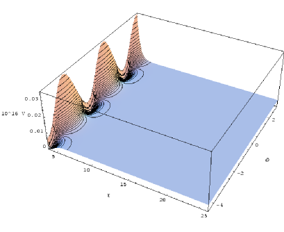
(a) (b)

Figure 4: (a) The $T_{2}$-potential surface $V(\tau,\theta)$ for the parameter set 1 of Table 1. Equipotential contour lines are superposed. Both $\tau$ and $\theta$ are multiplied by the characteristic scale $a_{2}$. The surfaces for the other parameter sets in the Table are very similar when $a_{2}$-scaled, even sets 5 and 6 with high $W_{0}$. In all cases, we manually uplifted the potential to have zero cosmological constant at the minimum. The periodicity in the axionic direction and the constancy at large $a_{2}\tau$ are manifest. If instead of $\tau$, we used the canonically-normalized field eq.(29) which is amplified by $\sqrt{\mathcal{V}}$, the undulating nature in $\theta$ at large $\varphi$ becomes more evident. However, the canonically-normalized inflaton is trajectory dependent and not a global function. (b) $V(\tau)$ for $\theta$ at $\cos(a_{2}\theta)=\pm 1$ shows how the flow for the positive value from large $\tau$ would be inward, but the flow would be outward for the negative value (and be unstable to $\theta$ perturbations). The dashed line is $V_{\infty}$, the $\tau\rightarrow\infty$ asymptote.

The potential eq.(26) has seven parameters $W_{0},a_{2},A_{2},\lambda_{2},\alpha,\xi$, and $g_{s}$ whose meaning was explained in § 2. We have investigated the shape of the potential $V(\tau,\theta)$ for a range of these parameters. $W_{0}$, $a_{2}$, $A_{2}$ control the low energy phenomenology of this model (see [20]) and are the ones we concentrate on here for our inflation application. We shall not deal with particle phenomenology aspects in this paper. Some choices of parameters $W_{0}$, $a_{2}$, $A_{2}$ seem to be more natural (see [20]). To illustrate the range of potentials, we have chosen the six sets of parameters given in Table 1. There is some debate on what are likely values of $W_{0}$ in string theory. We chose a range from intermediate to large. Since there are scaling relations among parameters, we can relate the specific ones we have chosen to others. An estimate of the magnitude of $W_{0}$ comes from a relation of the flux 3-forms $F_{3}$ and $H_{3}$ which appear in the definition of $W_{0}$ (eq.5) to the Euler characteristic $\tilde{\chi}$ of the F-theory 4-fold, which is $\tilde{\chi}\sim\int F_{3}\wedge H_{3}$ from the tadpole cancellation condition. This suggests an approximate upper bound $W_{0}\sim\sqrt{\tilde{\chi}}$ [11]. For typical values of $\tilde{\chi}\sim 10^{3}$, we would have $W_{0}\sim 10-100$. There are examples of manifolds with $\tilde{\chi}$ as large as $10^{6}$, which would result in $W_{0}\sim 10^{3}$. Further, the bound itself can be evaded by $F_{3}\wedge H_{3}=0$ terms. However, we do not wish to push $W_{0}$ too high so that we can avoid the effects of higher perturbative corrections. We can use the scaling property for the parameters to move the value of $W_{0}$ into a comfortable range. This should be taken into account while examining the table.

The parameter sets in the table can be divided into two classes: Trajectories in sets $1\dots 4$ produce a spectrum of scalar perturbations that is comparable to the experimentally observed one (good parameter sets), whereas trajectories in parameter set $5$ and $6$ produce spectra whose normalization is in disagreement with observations (bad parameter sets). Sets 3 and 4 were chosen to large values of $W_{0}$ to illustrate how things change with this parameter, but we are wary that with such large fluxes, other effects may come into play for determining the potential over those considered here. A typical potential surface $V(\tau,\theta)$ is shown in Fig. 4 with the isocontours of $V(\tau,\theta)$ superimposed.

The hypersurface $V(\tau,\theta)$ has a rich structure. It is periodic in $\theta$ with period $2\pi/a_{2}$, as seen in Fig 4. Along $\theta=\frac{\pi(2l+1)}{a_{2}}$, where $l$ is integer, the profile of the potential in the $\tau$ direction is that considered in [9]. It has a minimum at some $\tau=\tau_{min}$ and gradually saturates towards a constant value at large $\tau$, $V(\tau)\to V_{\infty}(1-Ca_{2}\tau e^{-a_{2}\tau})$, where $C$ is a constant. Along $\theta=\frac{2\pi l}{a_{2}}$, $V(\tau,\theta)$ falls gradually from a maximum at small $\tau$ towards the same constant value, $V(\tau)\to V_{\infty}(1+Ca_{2}\tau e^{-a_{2}\tau})$. Trajectories beginning at the maximum run away towards large $\tau$. Fig. 8(b) shows these two one-dimensional sections of the potential. For all other values of $\theta$ the potential interpolates between these two profiles. Thus, at large $\tau$, the $V$ surface is almost flat but slightly rippled. At small $\tau$, the potential in the axion direction is highly peaked. Around the maximum of the potential it is locally reminiscent of the “natural inflation” potential involving a pseudo Goldstone boson [27] (except that $\theta$ and $\tau$ must be simultaneously considered), as well as the racetrack inflation potential [2, 3].

There are two approximate scaling symmetries in this model (in the asymptotics of (26) for $\mathcal{V}\gg\xi$), similar to those in [2],

$$a_{i}\rightarrow u^{-1}a_{i}\ ,\ (A_{i},W_{0},\xi)\rightarrow u^{3/2}(A_{i},W_{0},\xi)\ ,\ (\tau_{i},\theta_{i})\rightarrow u(\tau_{i},\theta_{i})\ ,\ (\lambda_{i},{\cal P}_{s},\epsilon)\rightarrow(\lambda_{i},{\cal P}_{s},\epsilon)\ ;$$

$$a_{i}\rightarrow a_{i}\ ,\ (A_{i},W_{0})\rightarrow v^{-3/2}(A_{i},W_{0})\ ,\ (\tau_{i},\theta_{i})\rightarrow(\tau_{i},\theta_{i})\ ,\ {\cal P}_{s}\rightarrow v^{3}{\cal P}_{s}\ ,\ (\lambda_{i},\xi,\epsilon)\rightarrow(\lambda_{i},\xi,\epsilon)\ .$$ (28)

which can be used to generate families of models, trading for example large values of $W_{0}$ for small values of $\tau$. For instance, applying the $u$ scaling to parameter set 1, we can push the value of $W_{0}$ down to $W_{0}\approx 2$, but at the same time pushing $\tau$ to lie in the range $\tau=0.1\dots 1.0$ during inflation, a range which is quite problematic since at such small $\tau$ higher order string corrections would become important.

More generally, for the supergravity approximation to be valid the parameters have to be adjusted to have $\tau_{min}$ at least a few: $\tau$ is the four-cycle volume (in string units) and the supergravity approximation fails when it is of the string scale. However, even if the SUGRA description in terms of the scalar potential is not valid at the minimum, it still can be valid at large $\tau$, exactly where we wish to realize inflation. The consequence of small $\tau_{min}$ is that the end point of inflation, i.e. preheating, would have to be described by string theory degrees of freedom. We will return to this point in the discussion.

5.1 The Canonically-normalized Inflaton

If we define a canonically-normalized field $\varphi$ by $d\varphi^{2}/2=K_{22}d\tau^{2}$, then

$$\varphi=\sqrt{\frac{4}{3}\frac{\alpha\lambda_{2}}{\mathcal{V}+\frac{\xi}{2}}}\left(\frac{\tau}{\ell_{s}^{4}}\right)^{3/4}M_{p}.$$ (29)

It is therefore volume-suppressed. For inflation restricted to the $\tau_{2}$ direction, we identify $\varphi$ with the inflaton. The field change $\Delta\varphi$ over the many inflationary e-foldings $N\equiv-\ln a/a_{end}$ is given in the last column in Table 1 for a typical radial ($\tau$) trajectory. It is much less than $M_{p}$. (Here the scale factor at the end of inflation is $a_{end}$ so $N$ goes in the opposite direction to time.) The variations of the inflaton and the Hubble parameter wrt $N$,

$${d\varphi/M_{p}\over dN}=\sqrt{2\epsilon}\,,$$ (30)

$${d\ln H/M_{p}\over dN}=\epsilon\ ,\epsilon\equiv 1+q\,,$$ (31)

suggest we must have a deceleration parameter $q$ nearly the de Sitter $-1$ and the Hubble parameter $H$ nearly constant over the bulk of the trajectories. This is shown explicitly in § 6 and Figures 8 and 9. The parameter $\epsilon(N)$ is the first “slow-roll parameter”, although it only needs to be below unity for inflation. With $\epsilon$ so small, we are in a very slow-roll situation until near the end of inflation when it rapidly rises from approximately zero to unity and beyond.

Equation (30) connects the change in the inflaton field to the tensor to scalar ratio $r={\cal P}_{t}/{\cal P}_{s}$, since to a good approximation $r\approx 16\epsilon$. Since we find $\epsilon\ll 1$, we get very small $r$. The following relation [29, 30] gives a lower limit on the field variation in order to make tensor modes detectable

$$\frac{\varphi}{M_{\mathrm{pl}}}\approx 0.46\sqrt{\frac{r}{0.7}}\ .$$ (32)

We are not close to this bound. If $\varphi/M_{p}$ is restricted to be $<1$ in stringy inflation models, getting observable gravity wave signals is not easy. (A possible way out is to have many fields driving inflation in the spirit of assisted inflation [31].)

When the trajectory is not in the $\tau$ direction, the field identified with the canonically-normalized inflaton becomes trajectory-dependent as we describe in the next section and there is no global transformation. That is why all of our potential contour plots have focused on the Kähler modulus and its axion rather than on the inflaton.

6 Inflationary Trajectories

6.1 The Inflaton Equation of Motion

We consider a flat FRW universe with scalar factor $a(t)$ and real fields $(\tau,\theta)$. To find trajectories, we derive their equations of motion in the Hamiltonian form starting from the four dimensional Lagrangian (see [25] and references therein)

$${\cal L} = \sqrt{-g}\left(R+G_{ij}\dot{\phi}^{i}\dot{\phi}^{j}-V\right),$$ (33)

with canonical momentum $P_{i}=\frac{\partial{\cal L}}{\partial\dot{\phi}^{i}}=2a^{3}G_{ij}\dot{\phi}^{i}$, where we used $\sqrt{-g}=a^{3}$ and $\phi_{i}$, $i=1,2$ stands for $(\tau,\theta)$. (The usual field momentum is $P_{i}/a^{3}$.) Here the non-canonical kinetic term is

$$G_{ij}=K_{2\bar{2}}\delta_{ij},\ K_{i{\bar{j}}}=\frac{\partial^{2}K}{\partial T^{i}\partial\bar{T}^{\bar{j}}}.$$ (34)

The Hamiltonian is

$$\mathcal{H}=P_{i}\dot{\phi}^{i}-{\cal L}=\frac{1}{a^{3}}G^{ij}P_{i}P_{j}+V\,,$$ (35)

where $G^{ij}=G_{ij}^{-1}$. The equations of motion follow from $\dot{\phi}^{i}=\frac{\partial\mathcal{H}}{\partial P_{i}},\dot{P_{i}}=-\frac{\partial\mathcal{H}}{\partial\phi^{i}}$, which reduce to

$$\dot{\phi}^{i}=\frac{1}{2a^{3}}G^{ij}P_{j}\ ,\ \dot{P}_{i}=-\frac{1}{4a^{3}}\frac{\partial G^{kl}}{\partial\phi^{i}}P_{k}P_{l}-a^{3}\frac{\partial V}{\partial\phi^{i}}\ ,\ \dot{a}=aH\ ,\ \dot{H}=-\frac{1}{4a^{6}}G^{ij}P_{i}P_{j}\ .$$ (36)

We also use the constraint equation

$$M_{P}^{2}H^{2} = \frac{1}{3}\left(\frac{1}{4a^{6}}G^{ij}P_{i}P_{j}+V\right)=M_{P}^{2}H^{2}\epsilon/3+V/3$$ (37)

to monitor the accuracy of the numerical integration routine. Note that the deceleration, eq.(31), is related to the non-canonical kinetic term in the implicit manner indicated.

The inflaton is defined to be the field combination along the classical (unperturbed) trajectory. Isocurvature (isocon) degrees of freedom are those perpendicular to the classical trajectory. The kinetic metric in $M_{P}$ units is $d\psi^{2}=G_{ij}d\phi^{i}d\phi^{j}/M_{P}^{2}$. If $\theta$ is fixed, then $\psi$ is related to $\varphi$ introduced in § 5.1 by $\psi=\varphi/(\sqrt{2}M_{P})$. More generally, the inflaton between the initial condition $\phi^{i}(N_{0})$ and the value $\phi^{i}(N_{1})$ is the distance along the path, $\int d\psi$. For our case with diagonal $G_{ij}$, it is

$$\psi=\int\sqrt{K_{2\bar{2}}}d\tau(1+d\theta^{2}/d\tau^{2})^{1/2}\,.$$ (38)

6.2 Stochastic Fluctuations and CMB and LSS Constraints

The classical trajectory is perturbed by zero point fluctuations in all fields present, but only degrees of freedom with small mass will be relevant, hence in $\tau$ and $\theta$, which in turn influence the scalar metric fluctuations encoded in $\ln a=-N$, and in the gravitational wave degrees of freedom. Structure formation depends upon the fluctuations in the scalar 3-curvature, which are related to those in $\ln a$ measured on uniform Hubble surfaces [32, 33], $\delta{}^{(3)}R=4(k/a)^{2}\delta\ln a|_{H}$. The usual result for single-field inflation is motivated by stochastic inflation considerations: the zero point fluctuations in the inflaton at “horizon crossing” when the three-dimensional wavenumber $k\approx Ha$ are $\delta\psi=[H/(2\pi M_{P})]/\sqrt{2}$. Equation (30) gives the mapping, $\delta\ln a|_{H}=\delta\psi/\sqrt{\epsilon}$ along the inflaton direction. Thus the scalar power spectrum is

$${\cal P}_{s}\equiv k^{3}/(2\pi^{2})<|\delta\ln a|_{H}(k)|^{2}>=[H/(2\pi M_{P})]^{2}/(2\epsilon)\ e^{2u_{s}}\,,$$ (39)

where $u_{s}$ encodes small corrections to this simple stochastic inflation Hawking temperature formula.

The graviton zero point oscillations are, like those in a massless scalar field, proportional to the Hawking temperature at $k=Ha$,

$${\cal P}_{t}(k)=16\,[H/(2\pi M_{P})]^{2}/2\ e^{2u_{t}}\,.$$ (40)

where $u_{t}$ also encodes small corrections. The ratio $r(k)$ is therefore $\approx 16\epsilon$.

The scalar spectral index is given by $n_{s}-1=d\ln{\cal P}_{s}/d\ln k$. At lowest order, and for small $\epsilon$, it is $n_{s}-1=-2\epsilon-\epsilon^{\prime}/\epsilon$, where $\epsilon^{\prime}\equiv d\epsilon/d\ln a$. To have $\epsilon$ nearly zero as our trajectories do, and yet have $n_{s}$ differing at the 2-sigma level from unity as the current cosmic microwave background (CMB) and large scale clustering data indicate, imposes a constraint on $\epsilon^{\prime}/\epsilon$ which might seem to require a fine-tuning of the potential.

The current best estimate of $n_{s}$ in flat universe models characterized by six parameters, in which gravity waves are ignored, is $0.96\pm 0.017$ with CMB only, and $0.958\pm 0.015$ with CMB and large scale structure (LSS) clustering data [34]. The errors are Bayesian 1-sigma ones. For future reference, we note that the CMB data prefer a running of the scalar index at about the 2-sigma level, $dn_{s}/d\ln k=-0.047\pm 0.021$ at a pivot point $k_{p}=0.05\,{\rm Mpc}^{-1}$. However, the 6 parameter case with no running is a very good fit, except in the low $\ell$ regime. The preferred amplitude of the scalar perturbations is ${\cal P}_{s}(k_{p})=[21^{+1.3}_{-1.0}]\times 10^{-10}$. It is interesting to note that this number has been stable for a long time: the estimate from the COBE DMR experiment without the addition of any LSS or smaller scale CMB experiments was $[21\pm 3]\times 10^{-10}$ when extrapolated with this $n_{s}=0.96$ slope, and only slightly higher with no tilt [33].

The current constraint on the gravity wave contribution is ${\cal P}_{t}/{\cal P}_{s}<0.6$ at the 95% confidence limit with CMB data (with the powers evaluated at the pivot point $0.002\,{\rm Mpc}^{-1}$). When LSS data is added to the CMB, this drops to an upper limit of 0.28 but requires a single slope connection of the low $k$ regime in which the tensors can contribute to the CMB signal and high $k$ where the amplitude of LSS fluctuations is set. Relaxing this allows for higher values [10].

With the CMB-determined ${\cal P}_{s}$ estimate, we have $[H/(2\pi M_{P})]\approx 6.5\times 10^{-5}\sqrt{\epsilon}$. If the acceleration $\epsilon$ were uniform over the observable range and gave rise to this $n_{s}$, we would have $\epsilon=0.02$, $[H/(2\pi M_{P})]\approx 10^{-5}$ and $r\sim 0.3$. But our trajectories have $\epsilon$ nearly zero and $H$ almost flat, so to get the observed $n_{s}$ the observable range would have to be well into the braking period towards preheating: i.e., we would need $\epsilon^{\prime}/\epsilon\approx 0.04$ over the CMB+LSS window, which seems like it would require a very finely-tuned potential. Rather remarkably, the first cases we tried gave values near this at the relevant number of e-foldings before the end of inflation. This point was also made by Conlon and Quevedo [9] for pure $\tau$ trajectories. We also find there is room for modest running of the scalar index over the observable window. (Note that the tensor slope $n_{t}\equiv d\ln{\cal P}_{s}/d\ln k$ is $\approx-2\epsilon$, hence very small.) A consequence of the small $\epsilon$ is $[H/(2\pi M_{P})]\sim 10^{-10}$ and $V^{1/4}\sim 10^{14}\,{\rm Gev}$.

We caution that the single field model we used to estimate ${\cal P}_{s}$ includes fluctuations only along the trajectory. There will also be fluctuations perpendicular to it, and fluctuations in the parallel and perpendicular directions can influence each other. The latter are isocurvature degrees of freedom. Although these will leave the ${\cal P}_{t}$ formula unaffected, we expect modifications in the ${\cal P}_{s}$ formula, a point we return to after making an inventory of the sorts of trajectories that will arise.

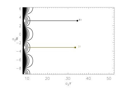
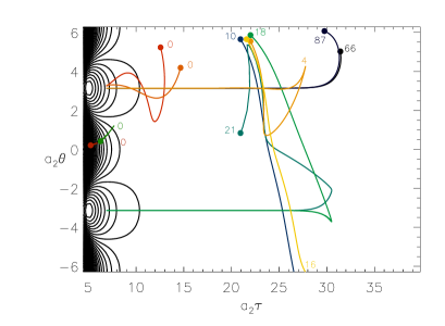
(a) (b)
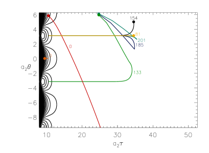
(c) (d)
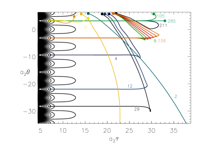
(e)

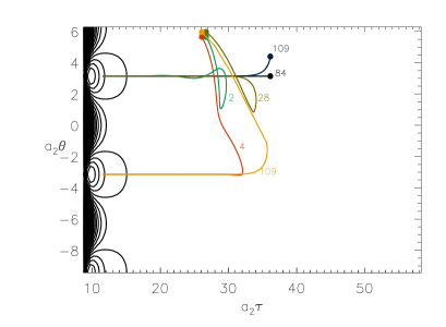
Figure 5: Contour-plots of the potential including trajectories for several choices of initial values (denoted by filled circles) in field space $(\tau,\theta)$. The trajectories are evolved numerically until inflation ends at $\epsilon=1$. The number of e-folds is indicated next to the corresponding trajectory. During the last stages of inflation, the field always rolls along one of the valleys towards the minima which are located in the centre of the white circles. The maxima are located in the dark spots. Inflation in the axion direction can significantly enhance the amount of inflation over that obtained in pure $\tau$ inflation. Trajectories starting at large $\tau$ roll to the nearest valley, then to the minimum. But starting at intermediate $\tau$ with the axion sufficiently far from its minimum, we find the field can cross several $\theta$-ridges before settling into a valley. Another manifestation is the run-away character for $\tau$ if the axion is placed close to its maximum. (a) shows the simple pure-$\tau$ inflation if $\theta$ is set to its minimum, as in Conlon and Quevedo, for parameter set 1. (b) shows the complex evolution for sample general starting conditions, for parameter set 1, (c), (d) and (e) show the same for sets 2, 3 and 4, respectively.

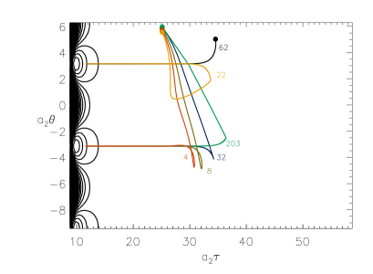
(a) (b)

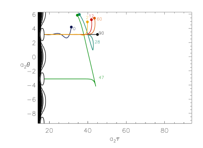
Figure 6: Sample trajectories for parameter sets 5 (a) and 6 (b), which have scalar power spectra amplitudes incompatible with the data. These still look similar to those in Fig. 5.

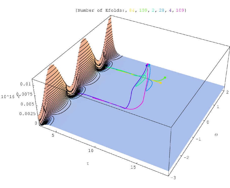
Figure 7: Potential with inflationary trajectories for parameter set 4. Shown is a plot of the potential in the $(\tau,\theta)$-plane, overlaid with equipotential contours. Note that for $\tau>5$ there are no contours because the potential is exponentially flat but it still has the periodic structure in the $\theta$-direction. The starting points of the trajectories are indicated by filled circles.

6.3 Trajectories with General Kähler modulus and Axion Initial Conditions

6.3.1 The $\tau$-valley Attractor

We first restrict ourselves to trajectories in $\tau$ to connect with the Conlon and Quevedo [9] treatment. The stable flow is in the $\theta=\frac{2\pi l}{a_{2}}$ trough. As can be seen in Fig. 5(a), enough e-foldings for successful inflation are possible provided one starts at large enough $\tau$. The dashed line in Fig. 8(a) shows $\epsilon$ is very small for this case, of order $\epsilon\approx 10^{-10}$. For the parameters we have considered, no effective inflation is possible if we start inward of $\tau_{min}$ rather than outward.

Another class of $\tau$ trajectories are those along the “ridge” where $\theta=\frac{2\pi l}{a_{2}}$ gives a positive contribution to the potential. These are unstable to small displacements in the axion direction.

The $\tau$-trough trajectories serve as late-time attractors for initial conditions that begin with $\theta$ out of the trough. The very flat profile of the potential at large $\tau$ allows for a regime of self-reproducing inflation (§ 7). Trajectories which originate in the self-reproducing regime invariably flow to the $\tau$-valley attractor and the observed e-folds would be just those of the Conlon and Quevedo sort.

6.3.2 The Variety of “Roulette” $\tau$-$\theta$ Trajectories

When we allow the initial values of $\tau$ and $\theta$ to be populated with an equal a priori probability prior, given a set of parameters defining the $V(\tau,\theta)$ surface, we encounter a wide range of inflationary trajectories. Examples of the variety of behaviours for the parameter sets given in Table 1 are shown for $\tau(\ln a),\theta(\ln a)$ in Figures 5 and 6, and for $H(\ln a),\epsilon(\ln a)$ in Figures 8 and 9. Some of the trajectories are predominantly $\theta$ ones before settling into a $\tau$-valley, similar to a roulette ball rotation before locking into a slot with a specific number, hence the name roulette inflation.

We began with the momenta of the fields set to zero, but the momenta are very quickly attracted to their slow-roll lock-in values, on of order an e-fold. We do not show this settling down phase in the trajectories we have plotted. We find a large fraction of trajectories are indeed inflating, and have the required $>40-50$ e-folds of inflation (§ 6.3.4) to give homogeneity and isotropy over our observable Hubble patch. Large enhancements of the number of e-folds over $\tau$-only inflation can occur because of significant flows in the $\theta$-direction, while $\tau$ evolves slowly. As the figures show, initial values starting far out in $\tau$ generally roll towards the nearest $\tau$-valley and then proceed along the $\tau$-attractor. Trajectories starting at intermediate $\tau$ have enough energy to pass through the $\tau$-valley in the axionic direction, but often turn around before reaching the neighbouring ridge, and roll back into the valley. They can move to larger $\tau$ while in the axion-dominated flow. If the initial values are chosen such that the initial potential energy is just a little higher, the inflaton can climb over the next ridge and settle in the adjacent valley, or the next one, or the next. Thus there exists bifurcation points which divide the phase space into solutions ending up in different valleys. Another feature in Fig. 5 is the existence of areas in which tiny changes in initial positions can lead to dramatic changes in the number of e-folds produced.

There are also cases in which the $\tau$-attractor is not reached before the end of inflation. When starting from moderate values in $\tau$, relatively far away from the valley, the field oscillates in the $\theta$ direction, albeit producing only a very small number of e-folds $N<1$ (see Fig. 5 for examples).

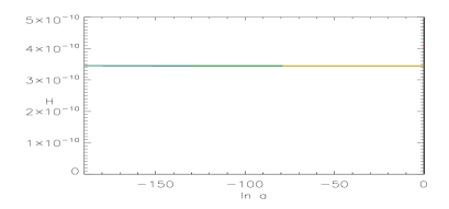
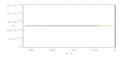
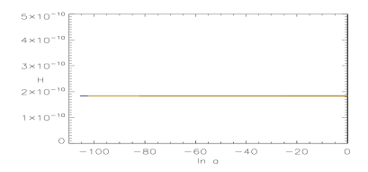
(a1) (a2)
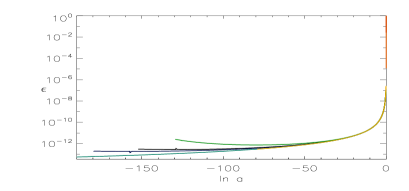
(b1) (b2)
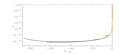
(c1) (c2)
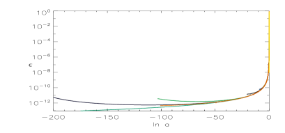
(d1) (d2)

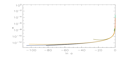
Figure 8: Hubble parameter $H(\ln a)$ (left column) and deceleration parameter $\epsilon(\ln a)$ (right column) as a function of the number of e-folds. $H(\ln a)$ is practically constant during inflation. $\epsilon$ during inflation is tiny and generally turns up towards the reheating phase rather rapidly. (a) Parameter set 1: the coloured trajectories are for general $(\tau,\theta)$ inflation, the dashed trajectory is inflation strictly along $\tau$ (b,c,d) are the same for sets 2, 3, 4, respectively. Note that units along the x-axes are $\ln a=-N\approx\ln k$ here and in the plots for the power spectra. There is a very rapid phase in which the trajectory settles down to an attractor for the $\tau$ and $\theta$ field momenta which we do not show.

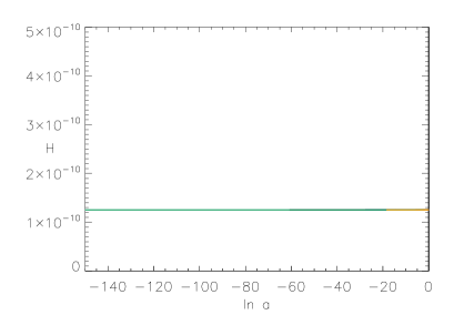
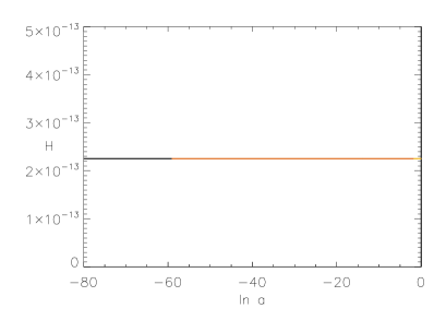
(a1) (a2)
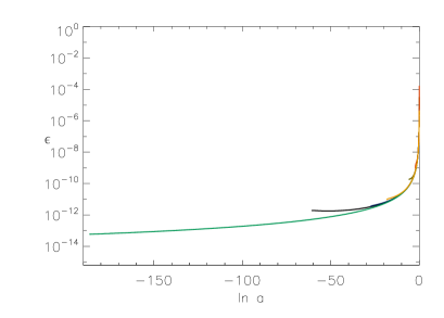
(b1) (b2)

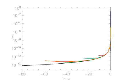
Figure 9: Same as Fig. 8, but for parameter sets 5 (a) and 6 (b).

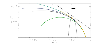
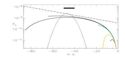
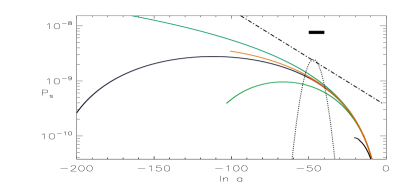
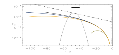
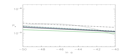
(a1) (a2)
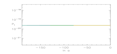
(b1) (b2)
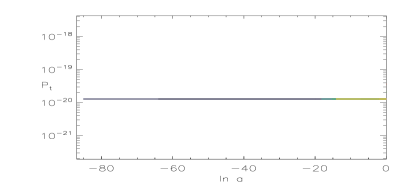
(c1) (c2)
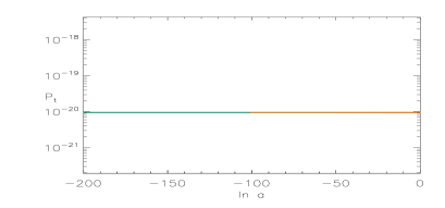
(d1) (d2)
(e) (f)

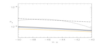
Figure 10: Power spectra for scalar ${\cal P}_{s}$ and tensor ${\cal P}_{t}$ fluctuations, derived assuming that only stochastic kicks along the trajectory are relevant for their determination, neglecting the influence of “isocurvature” fluctuations transverse to the inflaton trajectory. Both have amplitudes given by the instantaneous Hawking temperature. For comparison we present two template spectra: The dashed-dotted line shows a simple spectrum with no running of the spectral index $n_{s}=0.96$. The dotted line is a simple spectrum with running of the spectral index $n_{s}=0.91,dn_{s}/d\ln k=-0.044$, using values obtained by the ACBAR collaboration [34]. Both these spectra have the normalization set to ${\cal P}_{s}=2.1\times 10^{-9}$ at $N=45$. (a,b,c,d) are for parameter sets 1, 2, 3 and 4. The dashed line corresponds to inflation with $\theta=$const in the valley. Even though there is significant running for all models over large scales, the spectra are mostly featureless in the observable interval which panels (e) and (f) zoom into for sets 1 and 4.

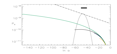
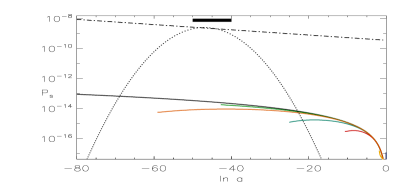
(a1) (a2)
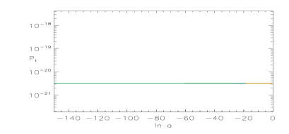
(b1) (b2)

Figure 11: Power spectra for potentials with parameter sets 5 and 6 that do not give a scalar amplitude near to the observed value.

6.3.3 The Scalar and Tensor Power Spectra and Isocurvature Effects

We estimate the power spectra ${\cal P}_{s}(k)$ using the single inflaton approximation, eq.(39), and ${\cal P}_{t}(k)$ using eq.(40), which only require $H$ and $\epsilon$ for each trajectory. These are shown in Figures 10 and Figures 11. As expected from the very small $\epsilon$’s we have encountered, to match ${\cal P}_{s}$ and hence $H^{2}/\epsilon$ to the data would require small $H$, low energy inflation, and hence very small gravity wave power, ${\cal P}_{t}\propto[H/M_{P}]^{2}$.

For comparison, Figures 10 and Figures 11 also show the best-fit scalar power spectra that were obtained by the ACBAR collaboration [34] using CMB and LSS clustering data. The fixed power law case has $n_{s}=0.96$. The spectrum with running has best-fits $n_{s}=0.911,dn_{s}/d\ln k=-0.044$. Obviously the running model can at best be valid only over a limited number of e-foldings. We indicate the observable range of e-foldings by the heavy black line in the power spectrum figures. As we show below, the mapping of wavenumber to number of e-foldings is imprecise but because the energy of inflation is low, the relevant range for CMB+LSS observables is in the range $N=-\ln a\in[40,50]$. For definiteness we take the pivot point $k_{p}$ for running to be at $N=45$.

To compute the scalar power spectra we assumed that the generation of fluctuations is driven by small perturbations along the trajectories, neglecting the effect of isocurvature fluctuations coming from perturbations perpendicular to this direction. We will now discuss why this might not necessarily catch the whole picture. In Fig 5d, there are a set of trajectories with initial values around $\tau\approx 21$ very close to each other where all fields end up in the second valley from the top. Two things are striking about those realizations of inflation: (1) the trajectories flange out when rolling down the axion towards larger $\tau$’s during the first part of their evolution; (2) the number of e-folds of inflation varies tremendously from as little as $N\approx 8$ all the way to $N\approx 106$ when going towards larger initial $\theta$’s while keeping $\tau$ fixed. The scalar spectra we compute for these flanging trajectories differ substantially, and make it clear that clear that our simple single field algorithm will be unjustified in some regions of the space of initial conditions. Even though the transverse quantum jitter is characterized by very small $H/M_{P}$ with width much smaller than the size of the curves in the figure, we recognize that tiny changes during the initial period of evolution in certain areas could produce big effects, an area for future investigation.

6.3.4 Number of e-folds $N$ and the wavenumber of perturbations

Since our trajectory computations are in terms of $\ln a/a_{end}$, whereas the observables probe $k\sim Ha$ in ${\rm Mpc}^{-1}$, we need to connect the two. The CMB+LSS probe $k$ from $\sim 10^{-4}\,{\rm Mpc}^{-1}$ to $\sim 1\,{\rm Mpc}^{-1}$, about 10 e-foldings. According to general lore (see e.g. [35]) the number of e-folds $N$ as a function of $k$ is given by

$$N(k)=62-{\rm ln}\frac{k}{6.96\times 10^{-5}\,{\rm Mpc}^{-1}}+\Delta,$$ (41)

where $6.96\times 10^{-5}{\rm Mpc}^{-1}$ is the inverse size of the present cosmological horizon and $\Delta$ is defined by the physics after inflation:

$$\Delta=-{\rm ln}\,\frac{10^{16}{\rm GeV}}{V_{k}^{1/4}}+\frac{1}{4}{\rm ln}\frac{V_{k}}{V_{\rm end}}-\frac{1}{3}{\rm ln}\frac{V^{1/4}_{\rm end}}{\rho_{\rm reh}^{1/4}}\ ,$$ (42)

where $\rho_{\rm reh}$ is the energy density at the end of reheating, $V_{k}$ is the value of the inflaton potential at the moment when the mode with the comoving wavenumber $k$ exits the horizon at inflation and $V_{\rm end}$ is the value at the end of inflation. We will not go into any details about this formula or its derivation, but merely motivate some numbers for the individual terms.

Starting with $\Delta$, we note that for its first term, $H\approx 3\times 10^{-10}M_{\mathrm{pl}}$ corresponds to $V_{k}^{1/4}\sim 10^{13}$ GeV. The second term can be neglected in our case, and the last term in the expression for $\Delta$ depends on the details of (p)reheating (which can be perturbative preheating, non-perturbative reheating or reheating involving KK-modes) which we put in the range of $1<\Delta<10$. Putting it all together we find that $\Delta\in[-17,-8]$. Therefore the observable range is about $10$ e-folds inside the interval [35,55], with the exact location of the former depending on the details of reheating. For the purpose of our discussion, we take the observable $N\in[40,50]$, and indicate this range by the black bar in Fig 10. We note that the required number of e-foldings is significantly lower than $65$.

7 Stochastic Regime of Self-Reproduction

Our potential is flattening exponentially rapidly as $\tau$ increases. Therefore the velocity of the fields which are placed at large enough $\tau$ will be rather small. This opens the possibility for stochastic evolution of the fields due to their quantum fluctuations dominating over classical slow-roll [36, 32]. We now show that in the model (4) there is region of $(\tau,\theta)$ space where the regime of self-reproduction operates. We distinguish this regime from the regime of eternal inflation due to bubble nucleations between different string vacua.

The criterion for self reproduction is actually that scalar perturbations are at least weakly nonlinear and that perturbation theory breaks down. The drift in each e-fold of the scalar $\phi^{i}$ is $\Delta\phi^{i}=G^{ij}(P_{j}/a^{3})/(2H)$ where $P_{j}/a^{3}$ is the canonically-normalized field momentum. The corresponding drift in the normalized inflaton $\psi$ is $\Delta\psi=\sqrt{\epsilon}$. The rms diffusion due to stochastic kicks is $\delta\psi=[H/(2\pi M_{P})]/\sqrt{2}$, as given in § 6.2. The rms kick beats the downward drift when ${\cal P}_{s}^{1/2}\approx[H/(2\pi M_{P})]/\sqrt{2\epsilon}$ exceeds unity, that is the fluctuations become non-perturbative. With such a flat nearly de Sitter potential, this is possible.

We now wish to consider this boundary as a function of $\theta$ as well as $\tau$. In general it is impossible to bring both of their kinetic terms simultaneously into canonical form. However, when we consider the fluctuations of fields, we can revert to the approximation in which the Kähler metric stays approximately constant over the time-scales of the fluctuations. The result is the following condition for the region where quantum fluctuations dominate over drift:

$$\frac{V}{12\pi^{2}}>\frac{1}{G_{\tau\tau}}\left(\frac{V_{,\tau}}{V}\right)^{2} \,\,\,\frac{V}{12\pi^{2}}>\frac{1}{G_{\theta\theta}}\left(\frac{V_{,\theta}}{V}\right)^{2}.$$ , (43)

This result is consistent with starting from $\ddot{\phi}^{i}+3H\dot{\phi}^{i}+\Gamma^{i}_{jk}\dot{\phi}^{j}\dot{\phi}^{k}+G^{ij}V_{,\phi^{j}}=0$, using slow-roll to neglect terms of $O(\dot{\phi}^{2},\ddot{\phi})$ and using the diagonality of $G$. In Fig. 12 we replot potential contours with various trajectories for parameter set 1, but with the drift/diffusion boundary now shown. Starting trajectories with arbitrary $\theta$ at the boundary should lead to large kicks in $\theta$ as well as $\tau$, but ultimately a settling into a $\tau$-trough well before the observable $N$ range is approached. In that case, the $\theta$ complexity of trajectories would not manifest itself.

Will the universe truly be in a stochastic regime of self-reproduction – the scenario of eternal inflation [37] – within such a model? The picture is of the last hole jittering about in size at $\tau$ far from the potential minimum. If the last hole can jitter about far away from equilibrium, then the same phenomenon would be expected for other holes that we took to be stabilized before the last stages of $T_{2}$ settle-down. In that case, it is unclear how the initial conditions for $T_{2}$ would be fed, but the most probable source of trajectories would not necessarily be from the $T_{2}$ self-reproduction boundary. In all cases, it is unclear whether further corrections to the potential way out there will uplift it to a level in which drift steps exceed diffusion steps. Fortunately, we are not dependent on such an asymptotically flat potential for the inflation model explored here to work.

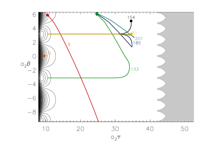
Figure 12: The self-reproduction region in which stochastic kicks dominate over the classical downward drift is indicated by the grey shaded area superposed upon the contour plot of the potential and some of its inflationary trajectories for parameter set 1. The most interesting trajectories start from outside of the quantum region. Those coming from the stochastic region will be attracted to the $\theta=\frac{2\pi l}{a_{2}}$ $\tau$-trough trajectories.

8 Discussion and Summary

We have investigated inflation in the “large volume” compactification scheme in the type IIB string theory model of [11, 12, 13]. Dynamics in the model are driven by Kähler moduli associated with four cycles and their axionic partners, $T_{i}=\tau_{i}+\theta_{i}$. We focused on the situation when all Kähler moduli/axions and the compact volume are stabilized at their minima except for a last modulus/axion pair $T_{2}=(\tau,\theta)$ which we identified with the “observed” early universe inflaton. We showed that $T_{2}$ dynamics does not perturb the global minimum of the total potential if $T_{2}$ operates on a lower energy scale than that associated with the earlier stabilizations. To do this, three or more moduli were needed. We explicitly demonstrated stabilization with a three field example, $T_{1},T_{2},T_{3}$. We also showed volume destabilization can occur even if it is initially stabilized if there are only two Kähler moduli, $T_{1},T_{2}$.

The two-dimensional potential $V(\tau,\theta)$ has a rich ridge-trough, hill-valley structure. We derived and solved the equations of motion of the $(\tau,\theta)$ system appropriate to an expanding universe using the Hamiltonian formalism of [25]. The non-canonical nature of the kinetic terms played an important role in defining the evolution.

The ensemble of inflationary trajectories is a rich set. We first studied inflation in the $\tau$ direction, along the valleys of the potential surface, which are late-time attractors for most of the general trajectories. For example, trajectories originating in the region of self-reproduction we identified in § 6.2 — where stochastic diffusive kicks can beat classical field drift — would invariably finish in the $\tau$-troughs. We calculated the number of e-folds $N$, the time variation of the Hubble parameter as a function of $\ln a$, $H(\ln a)$, the time variation of the acceleration history as encoded in the “first slow roll parameter” $\epsilon(\ln a)$, and the power spectrum for scalar ${\cal P}_{s}$ and tensor ${\cal P}_{t}$ fluctuations for many $\tau$-trajectories in the different realizations of the potential we explored. We can use the tools of single field inflation with confidence to compute the spectra if we are only following evolution of the inflaton within the Kähler modulus valley. Our results support the conclusions of Conlon and Quevedo [9] who first suggested this model of inflation. In particular, trajectories exist in the “prior” ensemble which satisfy the CMB+LSS data.

Our main objective was to study inflation with general initial conditions for $(\tau,\theta)$. We found that trajectories originating in elevated parts of the potential (near its maxima or its ridges) with moderate to large initial $\tau$ values can pass over many valleys and hills in $\theta$ before settling into a final $\tau$-valley approach to the end of inflation. These roulette wheel trajectories have an enhanced numbers of e-foldings relative to pure $\tau$ trajectories. No fine tuning of parameters was needed to get plenty of long-lasting inflation trajectories. In this respect, the Kähler modulus/axion inflation is superior to “better racetrack” inflation [3]. It is also preferable to have 200 good trajectories with a single complex field rather than one good trajectory with 200 complex fields as occurs in the string version [7] of “assisted inflation” [31]. The power spectra of scalar fluctuations for trajectories along a general direction need to be calculated using tools appropriate to multiple-field inflation. In order to estimate the amplitude we used expression (39) for single field stochastic inflation. We found indications of weak running in the spectral index over the observable range for some trajectories, and no running for others. To the extent that these single-inflaton estimations are reasonable, we again found plenty of roulette trajectories exist which satisfy the CMB+LSS data. Including the influence of the isocurvature degree of freedom on the observed power spectrum is needed to be completely concrete about such conclusions.

Although there can be pure $\tau$-trajectories, we have not found pure $\theta$ trajectories to be possible. The “natural inflation” model explored in [27] had a radial and an angular field, in a Mexican hat potential in which the Goldstone nature of the angular direction was broken into a $\cos(a_{2}\theta)$ type term only after the radial motion settled into the $\theta$-trough with random $\theta$ values. (The $a_{2}$ was also associated with non-perturbative terms similar to those invoked here.) The radial motion could come from either the small or large direction, the latter being like a chaotic inflation scenario for a first (unobserved) stage of inflation. The observed inflaton was to be identified with the angular motion from near a $\theta$ maximum, where some fraction of the random $\theta$ would reside, towards a $\theta$ minimum. One of the features of the model was that near the maximum one could use the potential shape to get small gravity waves and yet significant scalar tilts.

Why is our model so different? In a $\cos$ potential, inflation is possible in the immediate neighbourhood of the maximum, and so it is with our potentials if $\tau$ could be fixed. However we have found that beginning in the $\theta$ heights of our potentials near $\tau_{2,min}$ results in an outward radial flow, and, incidentally, insufficient e-folds to be of interest. These low $\tau$ heights are not populated from inward $\tau$-flows. This is because angular dynamics are intimately tied to radial dynamics since the symmetry breaking of $\theta$ and $\tau$ are due to the same process, so hills and valleys in $\theta$ are at all radii, ultimately guiding $\theta$ trajectories to the $\tau$-valleys. And our approach to the minimum is from a large radius flat potential rather than a growing chaotic inflation one. In general, we believe that our two-field Kähler modulus model gives a more natural inflation than natural inflation.

The inflaton potential at large $\tau$ is very shallow and in both the Kähler modulus and axion directions the motion rolls very slowly, even more so for larger $\tau$. In both $\tau$ and $\theta$ quantum kicks in the (quasi) de Sitter geometry can dominate over the classical slow roll drift. We identified this regime of the self-reproducing universe in our models.

However, to have a self-reproduction regime depends on the immunity of the model against perturbative corrections, as we discussed in § 3. Corrections may lead to polynomial terms in $\tau$ in $V(\tau,\theta)$ which may spoil the flatness, and possibly even spoil inflation itself. This problem is specific to the models of inflation associated with large $\tau$, as here. Models where inflation is realized with small values of the Kähler moduli, like “(better) racetrack inflation”, are not sensitive to the alteration of the potential at large $\tau$.

The issue is unclear because the exact form of the corrections is not yet known, so we are left with exploring the worst and the best case scenarios. The best case scenario is that corrections are absent or suppressed by a large volume factor $1/{\mathcal{V}}$. The worst case scenario is where corrections generate significant terms for large $\tau$. We note that inflation based on the potential $V(\tau,\theta)$ with two variables is more protected from the corrections than inflation based solely upon the potential $V(\tau)$. Indeed, if the potential $V(\tau,\theta)$ is altered, the runaway character along the $\tau$-ridges may be changed to give a shallow minimum along $\tau$, and the region around this minimum might turn out to provide another suitable terrain for inflationary behaviour if there is slow roll in the $\theta$ direction. Although asymptotic flatness and self-reproduction may be destroyed by induced masses, the observable window at significantly smaller $\tau$ may still allow inflations with enough e-foldings. As often happens in the investigation of string theory cosmology, assumptions such as the gentle nature of the uplift imposed here have to be made. That a viable stringy inflation seems feasible should motivate further work by the string theory community on the corrections and their role in inflation model building.

In this paper, we did not treat the issues of reheating at the end of inflation and the relation of the model to the observed particle physics. We just assumed that all the inflaton energy is transferred to the energy of ultra relativistic particles of the Standard Model. We require that there should be no overproduction of dangerous particles such as other long-lived moduli or (non LSP) gravitinos. Such dangerous relics may “overclose the universe” or decay late enough to destroy the success of the Big Bang Nucleosynthesis of the light elements. Details of reheating depend on the Kähler moduli dynamics at the end of inflation and on the interactions of the Kähler moduli with other fields, including the Standard Model particles. The dynamics of $\tau$ depends on the character of the potential around the minimum. In our picture all the other moduli except the inflaton $T_{2}$ are stabilized and stay at the global minimum. If the value of $\tau_{2,min}$ exceeds the string scale, the QFT description of the inflaton potential around the minimum will be valid, with the inflaton beginning to oscillate after slow roll ends. The coupling to other degrees of freedom, in particular those of the Standard Model, that appear in the reheating process is unclear. The canonically-normalized inflaton may have interaction via the gravitational coupling and this interaction must be sufficiently suppressed (e.g., by the volume $1/\mathcal{V}$) to avoid significant radiative corrections to the inflaton potential. On the other hand, the oscillating inflaton should decay into Standard Model particles fast enough (in $<100$ sec) to preserve successful Big Bang Nucleosynthesis. These requirements may put interesting constraints on the model for the couplings.

An alternative possibility is that $\tau_{2,min}$ is comparable to the string scale so that stringy effects play a direct role at the end of inflation. In this case one has to go beyond the QFT description of the processes. We note that small $\tau_{2,min}$ does not constrain the Kähler modulus/axion inflation, since the observed e-folds take place at large $\tau$: only the approach to, and consummation of, preheating would be affected, and would be quite different than in the QFT case. One may envisage the following as a possible scenario: the Kähler modulus, which corresponds to the geometrical size of the four-cycles, shrinks to a point corresponding to the disappearance of the hole. The energy of $\tau$ cascades first into the excited closed string loops, then further into KK modes in the bulk which interact with the Standard Model on the brane. Such a story is based on an analogy with the string theory reheating in warped brane inflation due to brane-antibrane annihilation investigated in [38]. In either the QFT or stringy case, reheating in Kähler moduli/axion inflation in the large volume stabilization model is an interesting and important question worthy of further study.

Even within the context of the Kähler modulus/axion model explored here, the statistical element of the theory prior probability in the landscape of late stage moduli is unavoidable, so the terminology “roulette inflation” is quite appropriate — quite aside from the specific roulette trajectories we have identified that have a dominant angular motion before settling into a $\tau$-trough on the way to the minimum. Within the landscape, we may have to be content with error bars on inflationary histories that have a very large “cosmic variance” due to the broad range of theory models and trajectories possible as well as the data errors due to cosmic microwave background and large scale structure observational uncertainties.

References

- [1] S. Kachru, R. Kallosh, A. Linde and S. P. Trivedi, Phys. Rev. D68, 046005 (2003) [hep-th/0301240].
- [2] J. J. Blanco-Pillado, C. P. Burgess, J. M. Cline, C. Escoda, M. Gomez-Reino, R. Kallosh, A. Linde, F. Quevedo, JHEP 0411, 063 (2004) [arXiv:hep-th/0406230].
- [3] J. J. Blanco-Pillado, C. P. Burgess, J. M. Cline, C. Escoda, M. Gomez-Reino, R. Kallosh, A. Linde, F. Quevedo, JHEP 0609, 002 (2006) [arXiv:hep-th/0603129].
- [4] S. Kachru, R. Kallosh, A. Linde, J. Maldacena, L. McAllister, S. P. Trivedi, JCAP 0310, 013 (2003) [hep-th/0308055].
- [5] K. Dasgupta, C. Herdeiro, S. Hirano and R. Kallosh, Phys. Rev. D 65, 126002 (2002) [arXiv:hep-th/0203019]; J. P. Hsu, R. Kallosh and S. Prokushkin, JCAP 0312, 009 (2003) [arXiv:hep-th/0311077]; K. Dasgupta, J. P. Hsu, R. Kallosh, A. Linde and M. Zagermann, JHEP 0408, 030 (2004) [arXiv:hep-th/0405247].
- [6] M. Alishahiha, E. Silverstein and D. Tong, Phys. Rev. D 70, 123505 (2004) [arXiv:hep-th/0404084]. A. Buchel and R. Roiban, “Inflation in warped geometries,” Phys. Lett. B 590, 284 (2004) [arXiv:hep-th/0311154]; C. P. Burgess, J. M. Cline, H. Stoica and F. Quevedo, “Inflation in realistic D-brane models,” JHEP 0409, 033 (2004) [arXiv:hep-th/0403119]; O. DeWolfe, S. Kachru and H. Verlinde, “The giant inflaton,” [arXiv:hep-th/0403123]; N. Iizuka and S. P. Trivedi, “An inflationary model in string theory,” Phys. Rev. D 70, 043519 (2004) [arXiv:hep-th/0403203].
- [7] R. Easther and L. McAllister, JCAP 0605, 018 (2006) [arXiv:hep-th/0512102].
- [8] L. A. Kofman, A. D. Linde and A. A. Starobinsky, Phys. Lett. B 157, 361 (1985).
- [9] J. P. Conlon and F. Quevedo, “Kähler Moduli Inflation” [arXiv:hep-th/0509012]
- [10] J. R. Bond, C. Contaldi, L. Kofman, P. M. Vaudrevange, “Scanning Inflation”, in preparation
- [11] V. Balasubramanian, P. Berglund, “Stringy corrections to Kähler potentials, SUSY breaking, and the cosmological constant problem,” JHEP 0411 (2004) 085, [arXiv:hep-th/0408054]
- [12] V. Balasubramanian, P. Berglund, J. P. Conlon and F. Quevedo, “Systematics of moduli stabilization in Calabi-Yau flux compactifications,” JHEP 0503 (2005) 007 [arXiv:hep-th/0502058]
- [13] J. P. Conlon, F. Quevedo and K. Suruliz, “Large-volume flux compactifications: Moduli spectrum and D3/D7 soft supersymmetry breaking” [arXiv:hep-th/0505076]
- [14] J. Simon, R. Jimenez, L. Verde, P. Berglund and V. Balasubramanian, arXiv:astro-ph/0605371.
- [15] R. Holman and J. A. Hutasoit, [arXiv:hep-th/0603246].
- [16] K. Becker, M. Becker, M. Haack and J. Louis, “Supersymmetry breaking and alpha’-corrections to flux induced potentials,” JHEP 0206, 060 (2002) [arXiv:hep-th/0204254].
- [17] E. Witten, “Nonperturbative superpotentials in string theory”, Nucl. Phys. B474 (1996) 343 [arXiv:hep-th/9604030].
- [18] S. B. Giddings, S. Kachru, J. Polchinski, Phys. Rev. D66, 106006 (2002) [hep-th/0105097].
- [19] P. S. Aspinwall and R. Kallosh, “Fixing all moduli for M-theory on K3 x K3,” JHEP 0510, 001 (2005) [arXiv:hep-th/0506014].
- [20] J. P. Conlon, S. S. Abdussalam, F. Quevedo and K. Suruliz, “Soft SUSY breaking terms for chiral matter in IIB string compactifications” [arXiv:hep-th/0610129].
- [21] P. Candelas and X. de la Ossa, “Moduli Space Of Calabi-Yau Manifolds,” Nucl. Phys. B 355, 455 (1991).
- [22] F. Denef, M. R. Douglas and B. Florea, “Building a better racetrack,” JHEP 0406, 034 (2004) [arXiv:hep-th/0404257].
- [23] P. Candelas, X. C. De La Ossa, P. S. Green and L. Parkes, “A Pair of Calabi-Yau Manifolds as an Exactly Soluble Superconformal Field Theory”, Nucl. Phys. B359 (1991) 21
-
[24]
M. Berg, M. Haack and B. Kors,
“String loop corrections to Kaehler potentials in orientifolds,”
JHEP 0511, 030 (2005)
[arXiv:hep-th/0508043];
“On volume stabilization by quantum corrections,” Phys. Rev. Lett. 96, 021601 (2006) [arXiv:hep-th/0508171]. - [25] R. Kallosh and S. Prokushkin, “Supercosmology” [arXiv:hep-th/0403060].
- [26] C. P. Burgess, R. Kallosh and F. Quevedo, “de Sitter string vacua from supersymmetric D-terms,” JHEP 0310, 056 (2003) [arXiv:hep-th/0309187].
- [27] F. C. Adams, J. R. Bond, K. Freese, J. A. Frieman and A. V. Olinto, Phys. Rev. D 47, 426 (1993) [arXiv:hep-ph/9207245]; K. Freese, J. A. Frieman and A. V. Olinto, Phys. Rev. Lett. 65, 3233 (1990).
- [28] A. A. Starobinsky, Phys. Lett. B 91, 99 (1980).
- [29] G. Efstathiou and K. J. Mack, JCAP 0505, 008 (2005) [arXiv:astro-ph/0503360].
- [30] D. H. Lyth, Phys. Rev. Lett. 78, 1861 (1997) [arXiv:hep-ph/9606387].
- [31] A. R. Liddle, A. Mazumdar and F. E. Schunck, Phys. Rev. D 58, 061301 (1998) [arXiv:astro-ph/9804177].
- [32] D.S. Salopek and J.R. Bond, Phys. Rev. D43, 1005-1031 (1991)
- [33] J.R. Bond, “Theory and Observations of the Cosmic Background Radiation”, Cosmology and Large Scale Structure 469-674(1996), Les Houches Session LX, August 1993, ed. R. Schaeffer, Elsevier Science Press.
- [34] C.L. Kuo, P.A.R. Ade, J.J. Bock, J.R. Bond, C.R. Contaldi, M.D. Daub, J.H. Goldstein, W.L. Holzapfel, A.E. Lange, M. Lueker, M. Newcomb, J.B. Peterson, C. Reichardt, J. Ruhl, M.C. Runyan, Z. Staniszweski , Ap.J., in press (2007) [arXiv:astro-ph/0611198].
- [35] D. I. Podolsky, G. N. Felder, L. Kofman and M. Peloso, Phys. Rev. D 73, 023501 (2006) [arXiv:hep-ph/0507096].
- [36] A. Linde, Phys. Lett. 175 (1986) 395; A. Linde, D. Linde and A. Mezhlumian, Phys. Rev. D 49, 1783 (1994) [arXiv:gr-qc/9306035].
- [37] A. D. Linde, Mod. Phys. Lett. A 1, 81 (1986).
- [38] N. Barnaby, C. P. Burgess and J. M. Cline, JCAP 0504, 007 (2005) [arXiv:hep-th/0412040]; A. R. Frey, A. Mazumdar and R. Myers, Phys. Rev. D 73, 026003 (2006) [arXiv:hep-th/0508139]; L. Kofman and P. Yi, Phys. Rev. D 72, 106001 (2005) [arXiv:hep-th/0507257]; X. Chen and S. H. Tye, JCAP 0606, 011 (2006) [arXiv:hep-th/0602136].