FTI/UCM 90-2006

The noncommutative $U(1)$ Higgs-Kibble model in the enveloping-algebra formalism and its renormalizability.

C.P. Martín, D. Sánchez-Ruiz and C. Tamarit Departamento de Física Teórica I, Facultad de Ciencias Físicas
Universidad Complutense de Madrid, 28040 Madrid, Spain

We discuss the renormalizability of the noncommutative $U(1)$ Higgs-Kibble model formulated within the enveloping-algebra approach. We consider both the phase of the model with unbroken gauge symmetry and the phase with spontaneously broken gauge symmetry. We show that against all odds the gauge sector of the model is always one-loop renormalizable at first order in $\theta^{\mu\nu}$, perhaps, hinting at the existence of a new symmetry of the gauge sector of the model. However, we also show that the matter sector of the model is non-renormalizable whatever the phase.

PACS: 11.10.Gh, 11.10.Nx, 11.15.-q.
Keywords: Renormalization, Regularization and Renormalons, Spontaneous symmetry breaking, Non-commutative geometry.

1 Introduction

At present, there is only one available framework to formulate gauge theories in noncommutative space-time for an arbitrary simple gauge group in an arbitrary representation. This very framework is the only known formalism where one may have fields with arbitrary $U(1)$ charge. The formalism we are referring to was introduced in refs. [1, 2] and [3] and led to the formulation of the noncommutative standard model [4] and some Grand Unification models [5]. Some phenomenological implications of these models have been studied recently [6, 7, 8, 9, 10, 11], but quite a lot of work remains to be done in view of the coming of the LHC.

As is well known, the Seiberg-Witten map plays a central role in the framework of refs. [1, 2] and [3]. Indeed, the noncommutative gauge fields are defined in terms of the ordinary fields by means of the formal series expansion in powers of the noncommutative matrix parameter $\theta^{\mu\nu}$ that implements the Seiberg-Witten map. The noncommutative gauge fields do not thus belong, in general, to the Lie algebra of the gauge group but are valued in the enveloping algebra –this is why the formalism is called the enveloping-algebra formalism– of that Lie algebra. This is quite at variance with the alternative approach to model building in noncommutative space-time employed in refs. [12, 13, 14] and [15].

The renormalizability of some noncommutative field theory models constructed within the enveloping-algebra formalism has been studied in a number of papers: see refs. [16, 17, 18, 19, 20, 21]. In all these papers, and throughout this one, it is assumed that both the quantization procedure and the renormalization program deal with the 1PI functions of the ordinary fields that define the noncommutative fields via the Seiberg-Witten map. The reader is referred to ref. [22] for an alternative interesting proposal. The models whose UV divergences have been worked out in refs. [16, 17, 18, 19, 20, 21] only have $U(1)$ and/or $SU(N)$ gauge fields and Dirac fermions in the fundamental representation. It turns out that at first order in $\theta^{\mu\nu}$, and against all odds, the one-loop UV divergences of the Green functions that only involve gauge fields in the external legs are renormalizable in the models that have and have not Dirac fermions. This is quite a surprising result since, as already pointed out in ref. [17], BRST invariance on its own cannot account for it, thus hinting at the existence of an as yet unveiled symmetry of the noncommutative gauge sector of these models. The result in question is even more surprising if one takes into account that the Green functions that carry fermion fields in the external legs cannot all be renormalized, thus rendering nonrenormalizable in the enveloping-algebra approach all the noncommutative models studied so far.

The main purpose of this paper is to see whether the results summarized in the previous paragraph also hold when the matter fields are not Dirac fermions but scalar fields –let us recall that the Higgs field is a key ingredient of the Standard Model. The simplest model that captures some of the features of the noncommutative Standard Model and includes both gauge fields and scalar fields is the noncommutative $U(1)$ Higgs-Kibble model. This model has a phase where the $U(1)$ symmetry is spontaneously broken and has also a phase where the $U(1)$ symmetry is not broken. The renormalization properties of the noncommutative $U(1)$ Higgs-Kibble model have never been studied when formulated within the enveloping-algebra formalism, although they have been analyzed within the standard noncommutative field theory formalism –see ref. [23] for the $U(1)$ Higgs-Kibble model and refs. [24, 25, 26, 27] for other models with spontaneous symmetry breaking.

The computation we are about to sketch is quite a daunting one since it demands the calculation of 94 1PI Feynman diagrams to tell whether the model is renormalizable in the phase with no symmetry breaking. In this phase, we discuss both the massive and massless cases. To deal with such a large number of Feynman diagrams we have used the algebraic manipulation package $\tt Mathematica$ [28]. Then, we shall use the results obtained in the phase with no symmetry breaking to analyze the renormalizablity of the model in the phase with spontaneous symmetry breaking.

The layout of this paper is as follows. In section 2, we define the classical noncommutative $U(1)$ Higgs-Kibble model and work out the action up to first order in $\theta^{\mu\nu}$. The renormalizability of the model in the phase with unbroken gauge symmetry is discussed in section 3. In section 4, we analyze the renormalizability of the model in the phase with spontaneous symmetry breaking. A summary of the results obtained in the paper is given in section 5. The Feynman rules and Feynman diagrams quoted in the paper can be found in the appendix.

2 The action. The Seiberg-Witten map

As it was stated in the introduction, our noncommutative field theory model will be the $U(1)$ Higgs-Kibble model. The model contains a noncommutative $U(1)$ gauge field $A_{\mu}$ and a noncommutative complex scalar field $\Phi$ coupled to $A_{\mu}$. The classical action of the model in terms of the noncommutative fields reads

$$S_{\rm class}=\int\!d^{4}\!x\,-\frac{1}{4}F_{\mu\nu}\star F^{\mu\nu}+(D_{\mu}\Phi)^{*}\star D^{\mu}\Phi-\mu^{2}\Phi^{*}\star\Phi-\frac{\lambda}{4}(\Phi^{*}\star\Phi)^{2},$$ (2.1)

where

$$D_{\mu}\Phi={\partial}_{\mu}\Phi-ieA_{\mu}\star\Phi,\quad F_{\mu\nu}={\partial}_{\mu}A_{\nu}-{\partial}_{\nu}A_{\mu}-ie[A_{\mu},A_{\nu}]_{\star}.$$

$e$ denotes the coupling constant of the gauge interaction. $\mu$ is the mass parameter and $\lambda$ stands for the coupling constant of the scalar self-interaction, which we shall take to be positive.

In the enveloping-algebra approach the noncommutative fields are defined in terms of the ordinary fields –the ordinary $U(1)$ gauge field $a_{\mu}$ and the ordinary complex scalar $\phi$ with $U(1)$ charge $e$– by means of the Seiberg-Witten map. It is the ordinary fields $a_{\mu}$ and $\phi$ that will be chosen as the field variables to be used to first quantize and then renormalize the theory.

At first order in $h\theta^{\mu\nu}$, the most general Seiberg-Witten map reads

$$\begin{array}[]{l}A_{\mu}=a_{\mu}-\frac{eh}{2}\theta^{\alpha\beta}a_{\alpha}(2\partial_{\beta}a_{\mu}-{\partial}_{\mu}a_{\beta})+h\partial_{\mu}H+hS_{\mu}+O(h^{2}),\\ \Phi=\phi-\frac{eh}{2}\theta^{\alpha\beta}a_{\alpha}\partial_{\beta}\phi+ihH\phi+hF+O(h^{2}),\\ H=x_{1}\,\theta^{\alpha\beta}{\partial}_{\alpha}a_{\beta}\\ S_{\mu}=\kappa_{1}\,\theta^{\alpha\beta}{\partial}_{\mu}f_{\alpha\beta}+\kappa_{2}\,{\theta_{\mu}}^{\beta}\partial^{\nu}f_{\nu\beta}+e\kappa_{3}\,{\theta_{\mu}}^{\nu}{\partial}_{\nu}(\phi^{*}\phi)+ie\kappa_{4}{\theta_{\mu}}^{\nu}(D_{\nu}\phi^{*}\phi-\phi^{*}D_{\nu}\phi),\\ F=e\kappa_{5}\theta^{\alpha\beta}f_{\alpha\beta}\phi,\end{array}$$ (2.2)

which has five parameters –four real parameters $\kappa_{1},\,\kappa_{2},\,\kappa_{3},\,\kappa_{4}$ and a complex parameter $\kappa_{5}$– labelling the ambiguity associated with field redefinitions. The real parameter $x_{1}$ parametrizes a gauge transformation of the fields.

For convenience, we introduce next the following basis $\{t_{i}\}_{i=1,\dots,9}$ of independent, modulo total derivatives, and gauge invariant monomials that are of order one in $h\theta^{\mu\nu}$ and have mass dimension equal to four:

$$\begin{array}[]{lll}t_{1}=\theta^{\alpha\beta}f_{\alpha\beta}f_{\rho\sigma}f^{\rho\sigma}&t_{2}=\theta^{\alpha\beta}f_{\alpha\rho}f_{\beta\sigma}f^{\rho\sigma}&t_{3}=\theta^{\alpha\beta}\phi^{*}\phi\,\square f_{\alpha\beta}\\ t_{4}=\theta^{\alpha\beta}(D_{\rho}\phi)^{*}\phi\,\partial^{\rho}f_{\alpha\beta}&t_{5}=\theta^{\alpha\beta}(D_{\alpha}\phi)^{*}\phi\,\partial_{\rho}{f_{\beta}}^{\rho}&t_{6}=\theta^{\alpha\beta}(D_{\rho}\phi)^{*}D^{\rho}\phi f_{\alpha\beta}\\ t_{7}=\theta^{\alpha\beta}(D_{\alpha}\phi)^{*}D^{\rho}\phi f_{\beta\rho}&t_{8}=\theta^{\alpha\beta}f_{\alpha\beta}\,(\phi^{*}\phi)^{2}&t_{9}=\mu^{2}\theta^{\alpha\beta}f_{\alpha\beta}\,\phi^{*}\phi.\\ \end{array}$$ (2.3)

Substituting first the Seiberg-Witten map of eq. (2.2) in the action in eq. (2.1) and then expanding in powers of $h\theta^{\mu\nu}$, one obtains

$$S_{\rm class}=S^{(0)}+hS^{(1)}+O(h^{2}),$$ (2.4)

where $S^{(0)}$ is the ordinary classical contribution,

$$S^{(0)}=\int\!d^{4}\!x\,-\frac{1}{4}f_{\mu\nu}f^{\mu\nu}+(D_{\mu}\phi)^{*}D^{\mu}\phi-\mu^{2}\phi^{*}\phi-\frac{\lambda}{4}(\phi^{*}\phi)^{2},$$ (2.5)

–now, $D_{\mu}=\partial_{\mu}-iea_{\mu}$– and $S^{(1)}$ has the following form in terms of the $t_{i}$s defined in eq. (2.3):

$$S^{(1)}=\int\!d^{4}\!x\,\frac{e}{8}\,t_{1}-\frac{e}{2}\,t_{2}+eC_{3}\,t_{3}+eC_{4}\,t_{4}+eC_{5}\,t_{5}+eC_{6}t_{6}+eC_{7}t_{7}+eC_{8}t_{8}+e\mu^{2}C_{9}t_{9},\$$ (2.6)

where

$$\begin{array}[]{lll}C_{3}=-\kappa_{5}^{*}-i\kappa_{1}-\frac{i}{2}\,(\kappa_{2}+\kappa_{4})+\frac{1}{2}\,\kappa_{3}&C_{4}=-\frac{1}{4}+2i\,\text{Im}\kappa_{5}-2i\kappa_{1}&C_{5}=-\frac{1}{2}+2i(\kappa_{2}+\kappa_{4})\\ C_{6}=-\frac{1}{4}+2\,\text{Re}\kappa_{5}&C_{7}=-1&C_{9}=\frac{1}{4}-2\,\text{Re}\kappa_{5}\\ C_{8}=\frac{e^{2}}{2}\,\kappa_{3}-\lambda(\text{Re}\kappa_{5}-\frac{1}{16}).\end{array}$$ (2.7)

3 The model in the phase with unbroken symmetry

In this section we shall show that the gauge sector of the model with unbroken gauge symmetry is one-loop renormalizable at first order in $h\theta^{\mu\nu}$, and that the matter sector is not renormalizable.

3.1 Feynman rules and one-loop UV divergences

In the case at hand $\mu^{2}\geq 0$, so that the classical vacuum of the theory is the trivial field configuration $\phi=0$ and $a_{\mu}=0$. To quantize the theory at first order in $h\theta^{\mu\nu}$, we shall add to the classical action in eq. (2.4) the gauge-fixing, $S_{\rm gf}$, and ghost, $S_{\rm gh}$, terms, to obtain

$$S=S_{\rm class}+S_{\rm gf}+S_{\rm gh}=S^{(0)}+hS^{(1)}+S_{\rm gf}+S_{\rm gh},$$ (3.8)

where

$$S_{\rm gf}=\int\!d^{4}\!x\,-\frac{1}{2\xi}\,({\partial}_{\mu}a^{\mu})^{2},\quad S_{\rm gh}=\int\!d^{4}\!x\,\bar{c}\partial^{2}\,c.$$

Recall that it is the ordinary fields $a_{\mu}$ and $\phi$ that furnish the field variables to be used to carry out the quantization process: in the path integral we shall integrate over $a_{\mu}$ and $\phi$. Notice that for our choice of gauge fixing, the ghost fields, $c$ and $\bar{c}$, do not couple either to $a_{\mu}$ or to $\phi$, and hence we will dispose of them.

The Feynman rules that the action in eq. (3.8) gives rise to are depicted in figure 1 of the appendix, where the following notation is used for propagators and vertices:

Propagators

$$\begin{array}[]{l}a_{\mu}\longrightarrow G^{\mu\nu}(k)=\frac{i}{k^{2}+i\varepsilon}\Big{[}-g^{\mu\nu}+(1-\xi)\frac{k^{\mu}k^{\nu}}{k^{2}}\Big{]}\\ \phi\longrightarrow G(k)=\frac{i}{k^{2}-m^{2}+i\varepsilon}\end{array}$$

Ordinary vertices

$$\begin{array}[]{lll}\Gamma^{t(0)\,\mu}_{(1,1)}[r;p,q]=ie(p^{\mu}+q^{\mu})&\Gamma^{t(0)\,\mu\nu}_{(2,1)}[r,s;p,q]=2ie^{2}g^{\mu\nu}&\Gamma^{t(0)}_{(0,2)}[r,s;p,q]=-i\lambda\end{array}$$

Noncommutative vertices

$$\begin{array}[]{l}\Gamma^{t(1)\,\mu}_{(1,1)}[r;p,q]=\\ e\Big{[}-2C_{3}\theta^{\alpha\mu}(p-q)_{\alpha}(p-q)^{2}+2C_{4}\theta^{\alpha\mu}(p-q)_{\alpha}(p-q)\cdot p-C_{5}\theta^{\alpha\beta}p_{\alpha}q_{\beta}(p-q)^{\mu}\\ \phantom{e\Big{[}}-C_{5}\theta^{\alpha\mu}p_{\alpha}(p-q)^{2}+2C_{6}\theta^{\alpha\mu}(p-q)_{\alpha}p\cdot q+C_{7}\theta^{\alpha\beta}p_{\alpha}(p-q)_{\beta}q^{\mu}-C_{7}\theta^{\alpha\mu}p_{\alpha}q\cdot(p-q)\\ \phantom{e\Big{[}}+2C_{9}\mu^{2}\theta^{\alpha\mu}(p-q)_{\alpha}\Big{]}\\ \Gamma^{t(1)\,\mu\nu\eta}_{(3,0)}[p,q,r]=\\ -\frac{e}{2}\Big{[}2\theta^{\alpha\mu}p_{\alpha}(q\cdot rg^{\nu\eta}-q^{\eta}r^{\nu})+2\theta^{\alpha\nu}q_{\alpha}(r\cdot pg^{\eta\mu}-r^{\mu}p^{\eta})+2\theta^{\alpha\eta}r_{\alpha}(p\cdot qg^{\mu\nu}-p^{\nu}q^{\mu})\Big{]}\\ +e\Big{[}\theta^{\alpha\beta}p_{\alpha}q_{\beta}(r^{\mu}g^{\nu\eta}-r^{\nu}g^{\eta\mu})+\theta^{\alpha\beta}p_{\alpha}r_{\beta}(q^{\mu}g^{\nu\eta}-q^{\eta}g^{\mu\nu})+\theta^{\alpha\beta}q_{\alpha}r_{\beta}(p^{\nu}g^{\mu\eta}-p^{\eta}g^{\nu\mu})\\ \phantom{e\Big{[}}-\theta^{\alpha\nu}p_{\alpha}q^{\eta}r^{\mu}-\theta^{\alpha\eta}p_{\alpha}r^{\nu}q^{\mu}-\theta^{\alpha\eta}q_{\alpha}r^{\mu}p^{\nu}-\theta^{\alpha\mu}q_{\alpha}p^{\eta}r^{\nu}-\theta^{\alpha\mu}r_{\alpha}p^{\nu}q^{\eta}-\theta^{\alpha\nu}r_{\alpha}q^{\mu}p^{\eta}\\ \phantom{e\Big{[}}-q_{\beta}p\cdot r(\theta^{\mu\beta}g^{\nu\eta}+\theta^{\eta\beta}g^{\nu\mu})-r_{\beta}p\cdot q(\theta^{\mu\beta}g^{\eta\nu}+\theta^{\nu\beta}g^{\eta\mu})-p_{\beta}q\cdot r(\theta^{\nu\beta}g^{\mu\eta}+\theta^{\eta\beta}g^{\mu\nu})\\ \phantom{e\Big{[}}+\theta^{\mu\nu}(p\cdot rq^{\eta}-q\cdot rp^{\eta})+\theta^{\mu\eta}(p\cdot qr^{\nu}-r\cdot qp^{\nu})+\theta^{\nu\eta}(q\cdot pr^{\mu}-r\cdot pq^{\mu})\Big{]}\\ \Gamma^{t(1)\,\mu\nu}_{(2,1)}[r,s;p,q]=\\ e^{2}\Big{[}C_{4}(2\theta^{\alpha\nu}s^{\mu}s_{\alpha}+2\theta^{\alpha\mu}r^{\nu}r_{\alpha})+C_{5}(\theta^{\mu\beta}s^{\nu}s_{\beta}+\theta^{\nu\beta}r^{\mu}r_{\beta}-\theta^{\mu\nu}(s^{2}-r^{2}))\\ \phantom{e\Big{[}}+C_{6}(2\theta^{\alpha\nu}(q+p)^{\mu}s_{\alpha}+2\theta^{\alpha\mu}(q+p)^{\nu}r_{\alpha})+C_{7}(\theta^{\mu\beta}s_{\beta}q^{\nu}-\theta^{\mu\nu}q\cdot s+\theta^{\alpha\beta}p_{\alpha}s_{\beta}g^{\mu\nu}-\theta^{\alpha\nu}p_{\alpha}s^{\mu}\\ \phantom{e\Big{[}}+\theta^{\nu\beta}r_{\beta}q^{\mu}+\theta^{\mu\nu}q\cdot r+\theta^{\alpha\beta}p_{\alpha}r_{\beta}g^{\mu\nu}-\theta^{\alpha\mu}p_{\alpha}r^{\nu})\Big{]}\\ \Gamma^{t(1)\,\mu\nu\rho}_{(3,1)}[r,s,t;p,q]=\\ e^{3}\Big{[}4C_{6}(\theta^{\alpha\rho}g^{\mu\nu}t_{\alpha}+\theta^{\alpha\nu}g^{\mu\rho}s_{\alpha}+\theta^{\alpha\mu}g^{\nu\rho}r_{\alpha})+C_{7}(\theta^{\mu\beta}g^{\nu\rho}(t+s)_{\beta}+\theta^{\nu\beta}g^{\rho\mu}(r+t)_{\beta}\\ \phantom{e^{3}\Big{[}}+\theta^{\rho\beta}g^{\mu\nu}(s+r)_{\beta}-\theta^{\mu\rho}t^{\nu}-\theta^{\mu\nu}s^{\rho}-\theta^{\nu\mu}r^{\rho}-\theta^{\nu\rho}t^{\mu}-\theta^{\rho\nu}s^{\mu}-\theta^{\rho\mu}r^{\nu})\Big{]}\\ \Gamma^{t(1)\,\mu}_{(1,2)}[t;p,q;r,s]=8eC_{8}\theta^{\alpha\mu}t_{\alpha}.\end{array}$$ (3.9)

$C_{i}$, $i=1\dots 9$, have been given in eq. (2.6).

Now, using the fact that the BRST transformations of $a_{\mu}$ and $\phi$ read $sa_{\mu}=\partial_{\mu}c$ and $s\phi=ie\,\phi\,c$, respectively, it is not difficult to conclude that in dimensional regularization the pole part of the one-loop 1PI functional, $\Gamma[a_{\mu},\phi]_{\rm pole}^{\rm one-loop}$, must be gauge invariant. Hence, up to first order in $h\theta^{\mu\nu}$ this functional should read

$$\Gamma[a_{\mu},\phi,\phi^{*}]_{\rm pole}^{\rm one-loop}=\Gamma^{(0)}[a_{\mu},\phi,\phi^{*}]_{\rm pole}^{\rm one-loop}\,+\,h\,\Gamma^{(1)}[a_{\mu},\phi,\phi^{*}]_{\rm pole}^{\rm one-loop},$$ (3.10)

where

$$\begin{array}[]{l}\Gamma^{(0)}[a_{\mu},\phi,\phi^{*}]_{\rm pole}^{\rm one-loop}=\int\!d^{4}\!x\,\;-\frac{w_{1}}{4}f_{\mu\nu}f^{\mu\nu}+w_{2}\,(D_{\mu}\phi)^{*}\star D^{\mu}\phi-w_{3}\,\mu^{2}\phi^{*}\phi-w_{4}\,\frac{\lambda}{4}(\phi^{*}\phi)^{2},\\ \Gamma^{(1)}[a_{\mu},\phi,\phi^{*}]_{\rm pole}^{\rm one-loop}=\int\!d^{4}\!x\,\;\frac{e}{8}\,z_{1}\,t_{1}-\frac{e}{2}\,z_{2}\,t_{2}+\sum_{i=3}^{8}ez_{i}\,t_{i}+e\mu^{2}z_{9}t_{9}.\end{array}$$ (3.11)

The $t_{i}$s, $i=1\dots 9$, are the nine monomials in eq. (2.3), and $w_{i}$, $i=1\dots 4$, and $z_{i}$, $i=1\dots 9$, stand for coefficients that are simple poles in $\epsilon=D/2-2$.

Let $\Gamma_{(m,n)}^{\mu_{1}\dots\mu_{m}}[x_{k};y_{l};z_{l}]$ denote the 1PI Green function corresponding to $m$ $a_{\mu}(x)$ fields, $n$ $\phi^{*}(y)$ and $n$ $\phi(z)$ fields. Ignoring the tree-level ghost contribution, we have that the 1PI functional reads

$$\Gamma[a_{\mu},\phi,\phi^{*}]=\sum_{m,n}\frac{1}{m!(n!)^{2}}\int\prod_{k=1}^{m}\prod_{l=1}^{n}d^{D}x_{k}d^{D}y_{l}d^{D}z_{l}\Gamma_{(m,n)}^{\mu_{1}\dots\mu_{m}}[x_{k};y_{l};z_{l}]a_{\mu_{k}}(x_{k})\phi^{*}(y_{l})\phi(z_{l}).$$ (3.12)

The computation of the $w_{i}$s, $i=1,\dots,4$, in eq. (3.11) is a standard exercise in introductory courses to renormalization theory, so we will just quote the result:

$$w_{1}=-\frac{e^{2}}{48\pi^{2}\epsilon},\;w_{2}=\frac{e^{2}}{16\pi^{2}\epsilon}\,(3-\xi),\,w_{3}=-\frac{e^{2}\xi-\lambda}{16\pi^{2}\epsilon},\,w_{4}=\frac{1}{32\pi^{2}\epsilon}\,\Big{[}24\frac{e^{4}}{\lambda}-4e^{2}\xi+5\lambda\Big{]}.$$ (3.13)

The computation of the $z_{i}$s, $i=1,\dots,9$, in eq. (3.11) is, though, a very lengthy and involved computation since the pole part of a large number of topologically inequivalent diagrams –94 altogether– with a single noncommutative vertex –which is in general a long expression– must be worked out. It turns out that to obtain all the $z_{i}$s one must evaluate the pole part of the one-loop contributions to $\Gamma^{\mu\nu\rho}_{(3,0)},\,\Gamma^{\mu}_{(1,1)}$ and $\Gamma^{\mu}_{(1,2)}$ that are linear in $\theta^{\mu\nu}$ –see eq. (3.12) for notation. Let us next display the values of these one-loop pole parts that we shall denote, respectively, by $\Gamma^{(1)\mu\nu\rho}_{(3,0)}[p_{1},p_{2},-p_{1}-p_{2}]_{\rm pole}^{\rm one-loop}$, $\Gamma^{(1)\mu}_{(1,1)}[p_{1}-p_{2};p_{1},p_{2}]_{\rm pole}^{\rm one-loop}$ and $\Gamma^{(1)\mu}_{(1,2)}[p_{1}+p_{3}-p_{2}-p_{4};p_{1},p_{2},p_{3},p_{4}]_{\rm pole}^{\rm one-loop}$:

The $aaa$ 1PI Green function $\Gamma^{\mu\nu\rho}_{(3,0)}$.

There are 4 topologically inequivalent diagrams –see figure 2 in the appendix– contributing to the pole part of this Green function at first order in $h\theta^{\mu\nu}$, and they lead to the following result:

$$\Gamma^{(1)\mu\nu\rho}_{(3,0)}[p_{1},p_{2},-p_{1}-p_{2}]_{\rm pole}^{\rm one-loop}=-\frac{e^{2}}{48\pi^{2}\epsilon}\,\Gamma^{t(1)\mu\nu\rho}_{(3,0)}[p_{1},p_{2},-p_{1}-p_{2}],$$ (3.14)

where $\Gamma^{t(1)\mu\nu\rho}_{(3,0)}$ is the tree-level contribution given in eq. (3.9) coming from the contributions $t_{1}$ and $t_{2}$ to $S_{\rm class}$ –see eqs. (2.4) and (2.6).

The $a\phi^{*}\phi$ 1PI Green function $\Gamma^{\mu}_{(1,1)}$.

The pole parts of the 11 topologically inequivalent diagrams in figure 3 of the appendix are to be computed, to obtain the following answer:

$$\Gamma^{(1)\mu}_{(1,1)}[p_{1}-p_{2};p_{1},p_{2}]_{\rm pole}^{\rm one-loop}=\Gamma^{t(1)\,\mu}_{(1,1)}[\Delta_{3},\Delta_{4},\Delta_{5},\Delta_{6},\Delta_{7},\Delta_{9};\,p_{1}-p_{2};p_{1},p_{2}],$$ (3.15)

where $\Gamma^{t(1)\,\mu}_{(1,1)}[\Delta_{3},\Delta_{4},\Delta_{5},\Delta_{6},\Delta_{7},\Delta_{9};\,r;p,q]$ is obtained from $\Gamma^{t(1)\,\mu}_{(1,1)}[r;p,q]$ in eq. (3.9) by replacing $C_{i}$ with $\Delta_{i}$, $i=3,4,5,6,7$ and $9$, where

$$\begin{array}[]{l}\Delta_{3}=\frac{e^{2}}{192\pi^{2}\epsilon}[11+26C_{4}-13C_{5}-26C_{6}+13C_{7}-4C_{3}(1+3\xi)-\lambda(-12C_{3}+6C_{4}-3C_{5}-6C_{6}\\ \phantom{\Delta_{3}=\frac{e^{2}}{192\pi^{2}\epsilon}[}+2C_{7})]\\ \Delta_{4}=\frac{e^{2}}{32\pi^{2}\epsilon}[2-C_{5}+2C_{7}+2C_{4}(4-\xi)]\\ \Delta_{5}=\frac{e^{2}}{16\pi^{2}\epsilon}[2(1+C_{7})+C_{5}(3-\xi)]\\ \Delta_{6}=\frac{e^{2}}{32\pi^{2}\epsilon}[-1+C_{7}+2C_{6}(4-\xi)]\\ \Delta_{7}=\frac{e^{2}}{16\pi^{2}\epsilon}[4+C_{7}(7-\xi)]\\ \Delta_{9}=\frac{1}{32\pi^{2}\epsilon}[8C_{8}+e^{2}(-8C_{3}+4C_{4}-2C_{5}-2C_{6}+2C_{7}+2C_{9}(2-\xi))-\lambda(-4C_{6}+C_{7}-2C_{9})].\end{array}$$ (3.16)

The constants $C_{i}$, $i=3,4,5,6,7$ and $9$, are defined in eq. (2.7).

The $a\phi^{*}\phi\phi^{*}\phi$ 1PI Green function $\Gamma^{\mu}_{(1,2)}$.

Let $\Gamma^{t(1)\mu}_{(1,2)}[\Delta_{8};\,t;p,q;r,s]$ denote $\Gamma^{t(1)\mu}_{(1,2)}[t;p,q;r,s]$ in eq. (3.9), once $C_{8}$ is replaced with $\Delta_{8}$. Then, the computation of the pole part of the 79 topologically inequivalent diagrams in figure 4 of the appendix leads to the following equality:

$$\Gamma^{(1)\mu}_{(1,2)}[p_{1}+p_{3}-p_{2}-p_{4};p_{1},p_{2};p_{3},p_{4}]_{\rm pole}^{\rm one-pole}=\Gamma^{t(1)\mu}_{(1,2)}[\Delta_{8};\,p_{1}+p_{3}-p_{2}-p_{4};p_{1},p_{2};p_{3},p_{4}],$$ (3.17)

where

$$\begin{array}[]{l}\Delta_{8}=\frac{1}{256\pi^{2}\epsilon}\,[-4e^{4}(-12+4C_{3}-2C_{4}+C_{5}+26C_{6}-8C_{7})+5\lambda^{2}(4C_{6}-C_{7})\\ \phantom{\Delta_{8}=\frac{1}{256\pi^{2}\epsilon}\,[}-8e^{2}\lambda(8C_{3}-4C_{4}+2C_{5}+C_{6}-C_{7})+32e^{2}C_{8}(2-\xi)+80\lambda C_{8}].\end{array}$$ (3.18)

Taking into account eqs. (3.14), (3.15) and (3.17), one concludes that the $z_{i}$s, $i=1,\dots,9$, in eq. (3.11) are given by the following equalities:

$$z_{1}=z_{2}=-\frac{e^{2}}{48\pi^{2}\epsilon},\,z_{i}=\Delta_{i},\;\forall\,i=3\dots 9,$$ (3.19)

where the $\Delta_{i}$s, $i=3\dots 9$, are given in eqs. (3.16) and (3.18).

3.2 One-loop renormalization

Let us assume that the fields and parameters of the action in eq. (3.8) are the bare fields and parameters of the model. Then, as usual, we shall say that the model is one-loop multiplicatively renormalizable at first order in $h\theta^{\mu\nu}$, if the free coefficients of the counterterm action obtained by introducing the following renormalizations of the fields and parameters of the action in eq. (3.8)

$$\begin{array}[]{lll}a_{\mu}=Z_{a}^{1/2}a^{R}_{\mu}&\phi=Z_{\phi}^{1/2}\phi^{R}&e=Z_{e}e^{R}\\ \mu=Z_{\mu}^{1/2}\mu^{R}&\lambda=Z_{\lambda}\lambda^{R}&\xi=Z_{\xi}\xi^{R}\\ \theta=Z_{\theta}\theta^{R}&\kappa_{i}=\kappa_{i}^{R}+\delta\kappa_{i},\,i=1,2,3,4&\text{Re}\kappa_{5}=\text{Re}\kappa_{5}^{R}+\delta\text{Re}\kappa_{5}^{R}\\ \text{Im}\kappa_{5}=\text{Im}\kappa_{5}^{R}+\delta\text{Im}\kappa_{5}^{R}\end{array}$$ (3.20)

can be chosen to cancel the UV divergences of the 1PI functional given in eqs. (3.10), (3.11),
 (3.13) and (3.19).

Let $\delta Z_{a}=Z_{a}-1$, $\delta Z_{\phi}=Z_{\phi}-1$, $\delta Z_{e}=Z_{e}-1$, $\delta Z_{\mu}=Z_{\mu}-1$, $\delta Z_{\lambda}=Z_{\lambda}-1$, $\delta Z_{\xi}=Z_{\xi}-1$ and $\delta Z_{\theta}=Z_{\theta}-1$. Then, the multiplicative renormalization in eq. (3.20), when applied to the action in eq. (3.8), yields the following one-loop counterterm action up to first order in $h\theta^{\mu\nu}$:

$$S_{\rm ct}\,=\,S^{(0)}_{\rm ct}\,+\,h\,S^{(1)}_{\rm ct},$$

where

$$\begin{array}[]{l}S^{(0)}_{\rm ct}=\int\!d^{4}\!x\,-\frac{1}{4}\delta Z_{a}f_{\mu\nu}f^{\mu\nu}+\delta Z_{\phi}({\partial}_{\mu}\phi)^{*}\partial^{\mu}\phi-(\delta Z_{\phi}+\delta Z_{\mu})\mu^{2}\phi^{*}\phi\\ \phantom{S^{(0)}_{\rm ct}=}-ie(\delta Z_{\phi}+\delta Z_{e}+\frac{1}{2}\delta Z_{a}){\partial}_{\mu}\phi^{*}a^{\mu}\phi+ie(\delta Z_{\phi}+\delta Z_{e}+\frac{1}{2}\delta Z_{a})\phi^{*}a^{\mu}{\partial}_{\mu}\phi\\ \phantom{S^{(0)}_{\rm ct}=}+e^{2}(2\,\delta Z_{e}+\delta Z_{a}+\delta Z_{\phi})\phi^{*}\phi a_{\mu}a^{\mu}-\frac{\lambda}{4}(\delta Z_{\lambda}+2\delta Z_{\phi})(\phi^{*}\phi)^{2}-\frac{1}{2\xi}\,(\delta Z_{a}-\delta Z_{\xi})({\partial}_{\mu}a^{\mu})^{2},\\[10.0pt] S^{(1)}_{\rm ct}=\int\!d^{4}\!x\,\frac{e}{8}\,(\delta Z_{\theta}+\delta Z_{a})t_{1}-\frac{e}{2}(\delta Z_{\theta}+\delta Z_{a})t_{2}+e\sum_{i=3}^{7}[\delta C_{i}+C_{i}(\delta Z_{\theta}+\delta Z_{\phi})]t_{i}\\ \phantom{S^{(1)}=}+e[\delta C_{8}+C_{8}(\delta Z_{\theta}+2\delta Z_{\phi})]t_{8}+e\mu^{2}[\delta C_{9}+C_{9}(\delta Z_{\theta}+\delta Z_{\mu}+\delta Z_{\phi})]t_{9}.\end{array}$$ (3.21)

In the previous equation the fields $a_{\mu}$ and $\phi$ and the parameters $\mu^{2},e,\lambda$ and $\kappa_{i}$, $i=1,\dots 4$ are, respectively, the renormalized fields and parameters of eq. (3.20). We have suppressed the superscript “$R$” to make the notation simpler. To simplify the expression for $S^{(1)}_{\rm ct}$, the identity $\delta Z_{a}=-2\delta Z_{e}$, which is a consequence of the BRST invariance of the theory, has been used. Notice that as a consequence of the identities in eq. (2.7) the $\delta C_{i}$s in eq. (3.21) are defined by following equalities:

$$\begin{array}[]{ll}\delta C_{3}=-\delta\text{Re}\kappa_{5}+i\delta\text{Im}\kappa_{5}-\frac{i}{2}\,(\delta\kappa_{2}+\delta\kappa_{4})+\frac{1}{2}\,\delta\kappa_{3}-i\delta\kappa_{1}&\delta C_{4}=2i\delta\text{Im}\kappa_{5}-2i\delta\kappa_{1}\\ \delta C_{5}=2i(\delta\kappa_{2}+\delta\kappa_{4})&\delta C_{6}=2\delta\text{Re}\kappa_{5}\\ \delta C_{7}=0&\delta C_{9}=-2\delta\text{Re}\kappa_{5}\\ \delta C_{8}=\frac{1}{2}(2e^{2}\kappa_{3}\delta Z_{e}+e^{2}\delta\kappa_{3})-\lambda\delta Z_{\lambda}(\text{Re}\kappa_{5}-\frac{1}{16})-\lambda\delta\text{Re}\kappa_{5}.\end{array}$$ (3.22)

Of course, $\delta Z_{a}$, $\delta Z_{\phi}$, $\delta Z_{e}$, $\delta Z_{\mu}$, $\delta Z_{\lambda}$ and $\delta Z_{\xi}$ are the same as in the ordinary model, and in the MS scheme they read

$$\begin{array}[]{l}\delta Z_{a}=\frac{e^{2}}{48\pi^{2}\epsilon}=-2\delta Ze=\delta Z_{\xi},\quad\delta Z_{\phi}=-\frac{e^{2}(3-\xi)}{16\pi^{2}\epsilon},\\[8.0pt] \delta Z_{\mu}=\frac{3e^{2}-\lambda}{16\pi^{2}\epsilon}\quad\delta Z_{\lambda}=-\frac{1}{32\pi^{2}\epsilon}\,\Big{[}24\frac{e^{4}}{\lambda}-12e^{2}+5\lambda\Big{]}.\\ \end{array}$$ (3.23)

Next, in the MS scheme, $\delta Z_{\theta}$ and $\delta C_{i}$, $i=3,\dots,9$, of $S^{(1)}_{\rm ct}$ in eq. (3.21) must be chosen –were it possible– so that the sum $\Gamma^{(1)}[a_{\mu},\phi,\phi^{*}]_{\rm pole}^{\rm one-loop}+S^{(1)}_{\rm ct}$ vanishes. $\Gamma^{(1)}[a_{\mu},\phi,\phi^{*}]_{\rm pole}^{\rm one-loop}$ is given in eq. (3.11) and the values of its coefficients –the $z_{i}$s– are summarized in eq. (3.19). We thus conclude that $\delta Z_{\theta}$ must satisfy the following equalities:

$$-z_{1}=\delta Z_{\theta}+\delta Z_{a},\quad-z_{2}=\delta Z_{\theta}+\delta Z_{a},$$ (3.24)

whereas for $\delta C_{i}$, $i=3,\dots,9$ the following set of equations must hold:

$$\begin{array}[]{l}-z_{i}\,=\,\delta C_{i}\,+\,C_{i}(\delta Z_{\theta}+\delta Z_{\phi}),\quad i=3,4,5,6,7\\ -z_{8}=\delta C_{8}\,+\,C_{8}(\delta Z_{\theta}+2\,\delta Z_{\phi}),\\ -z_{9}=\delta C_{9}\,+\,C_{9}(\delta Z_{\theta}+\delta Z_{\mu}+\delta Z_{\phi}).\\ \end{array}$$ (3.25)

Taking into account eqs. (3.19) and (3.23), one concludes that the two equalities in eq. (3.24) hold if, and only if,

$$\delta Z_{\theta}=0.$$ (3.26)

This equation leads to the conclusion that $\theta^{\mu\nu}$ is not renormalized at the one-loop level in the MS scheme of dimensional regularization.

That the two equalities in eq. (3.24) hold is a necessary and sufficient condition for the gauge sector of our model –no matter fields in the external legs of the Green functions– to be multiplicatively renormalizable at one-loop and at first order in $\theta^{\mu\nu}$. BRST invariance does not imply that eq. (3.24) must be verified, since in our case the most general BRST invariant contribution involving only gauge fields reads up to first order in $h\theta^{\mu\nu}$:

$$\int\!d^{4}\!x\,\;-\frac{1}{4}\,w_{1}\,f_{\mu\nu}f^{\mu\nu}\,+\,h\,\frac{e}{8}\,z_{2}\,t_{1}\,-\,h\,\frac{e}{2}\,z_{3}\,t_{2},$$ (3.27)

Mark that the real numbers $w_{1}$, $z_{2}$ and $z_{3}$ are arbitrary. Now, only if $z_{2}=z_{3}$, it is possible to renormalize the $\theta^{\mu\nu}$ dependent part of the functional in the previous equation by means of the renormalization in eq. (3.20). Of course, we have shown by explicit computation that for our model $z_{2}=z_{3}$. But there is more: we have obtained not only that $z_{2}=z_{3}$, but that $z_{2}=z_{3}=w_{1}$. The latter train of equalities has nothing to do with the the gauge sector of the model being renormalizable at one loop, but with the fact that $\theta^{\mu\nu}$ is not renormalized at one-loop. We do not believe –following the author of ref. [17]– that this situation –that $z_{2}=z_{3}=w_{1}$– is an accident, but that it perhaps hints at the existence of an as yet unknown symmetry that mixes the three monomials in eq. (3.27). This symmetry must depend on $\theta^{\mu\nu}$, for it must relate monomials with different powers in $\theta^{\mu\nu}$. Notice that what we have obtained is that the renormalizability of the gauge sector of the model at one-loop and first order in $\theta^{\mu\nu}$ is governed by the renormalization of the coupling constant $e$ –recall that BRST invariance implies $\delta Z_{a}=-2\delta Z_{e}$.

Now, the matter sector of the model in the symmetric phase will be multiplicatively renormalizable –i.e by means of the renormalization transformations in eq. (3.20)– if, and only if, there exist $\delta\kappa_{i}$, $i=1,\dots,4$, $Re\delta\kappa_{5}$ and $Im\delta\kappa_{5}$ such that the set of eqs. (3.25) holds for them. Taking into account the values of the $z_{i}$s on the r.h.s of eq. (3.25) that are given in eqs. (3.19), (3.16) and (3.18), using the definitions of the $\delta C_{i}$s, $i=1,\dots,9$, provided in eq. (3.22), and recalling that the renormalized $C_{i}$s, $i=1,\dots,9$, are defined in terms of the renormalized $\kappa_{i}$, $i=1,\dots,5$, by the identities in eq. (2.7) and that the values of the $\delta Z$s are those in eqs. (3.23) and (3.26), one concludes, upon substitution of the previous results, that there is a unique set of parameters $\delta\kappa_{i}$, $i=1,\dots 5$, that solves the system of equations constituted by the first five –$i=3,4,5,6$ and $7$– equalities in eq. (3.25). This set of parameters reads

$$\begin{array}[]{l}\delta\kappa_{1}=\delta\text{Im}\kappa_{5}-\frac{e^{2}}{32\pi^{2}\epsilon}(2\kappa_{1}+\kappa_{2}-2\text{Im}\kappa_{5}+\kappa_{4})\\ \delta\kappa_{2}=-\delta\kappa_{4}\\ \delta\kappa_{3}=\frac{1}{192\pi^{2}\epsilon}[e^{2}(6+40\kappa_{3})-\lambda(1+12\kappa_{3})]\\ \delta\text{Re}\kappa_{5}=\frac{e^{2}}{128\pi^{2}\epsilon}(5-8\text{Re}\kappa_{5}).\end{array}$$ (3.28)

And yet, the full system of equations has no solution for $\mu^{2}\neq 0$, as the last equation –the equation with $z_{9}$ on the l.h.s– is not satisfied by the $\delta\kappa_{i}$s, $i=1,\dots,5$ in eq. (3.28). Indeed, upon substitution of those values in this last equation one obtains the constraint $6e^{2}-\lambda=0$. Notice that this constraint is not even renormalization group invariant, so it cannot be imposed in a renormalization group invariant way, precluding the implementation of the reduction-of-the-couplings mechanism of ref. [29] to dispose of the unwanted UV divergences. We thus conclude that the matter sector of the theory is not multiplicatively renormalizable if the scalar field is massive. If $\mu^{2}=0$, the last equality of eq. (3.25) need not be satisfied since, now, terms of the type $\mu^{2}t_{9}$ occur neither in the classical action nor in $\Gamma^{(1)}[a_{\mu},\phi,\phi^{*}]_{\rm pole}^{\rm one-loop}$ –see eq. (3.11). Unfortunately, the equation $-z_{8}=\delta C_{8}+C_{8}(\delta Z_{\theta}+2\delta Z_{\phi})$ is not satisfied by the parameters given in eq. (3.28), for its substitution in the latter equation leads to the constraint $204e^{2}-76e^{2}\lambda+15\lambda^{2}=0$. Remarkably, all dependence on the arbitrary parameters of the Seiberg-Witten map disappears, but the previous constraint is, of course, not valid for arbitrary $e$ and $\lambda$. The constraint is not even renormalization group invariant. In summary, the matter sector of our model is not multiplicatively renormalizable in the phase with no spontaneous symmetry breaking whatever the value of the mass.

We shall next address the issue of the non-multiplicative renormalizability of the model. We shall show that turning non-multiplicative –but local at every order in $\theta^{\mu\nu}$– the relationship between bare and renormalized fields will be of no avail in making the model renormalizable. Let us assume that the bare fields and renormalized fields are not related as in eq. (3.20), but as follows

$$a_{\mu}=a_{\mu}^{R}+\frac{1}{2}\,\delta Z_{a}\,a_{\mu}^{R}+h\delta Z_{\mu}[a_{\mu}^{R},\phi^{R},\phi^{R\,*},\partial,\theta^{\mu\nu}];\quad\phi=\phi^{R}+\frac{1}{2}\delta Z_{\phi}\,\phi^{R}+h\delta Z[a_{\mu}^{R},\phi^{R},\phi^{R\,*},\partial_{\mu},\theta^{\mu\nu}],$$

where

$$\begin{array}[]{l}\delta Z_{\mu}=x_{1}{\theta_{\mu}}^{\alpha}a_{\alpha}\phi^{*}\phi+x_{2}{\theta_{\mu}}^{\alpha}a_{\alpha}(\phi\phi+\phi^{*}\phi^{*})+ix_{3}{\theta_{\mu}}^{\alpha}a_{\alpha}(\phi\phi-\phi^{*}\phi^{*})+x_{4}{\theta_{\mu}}^{\alpha}({\partial}_{\alpha}\phi\phi+{\partial}_{\alpha}\phi^{*}\phi^{*})\\ \phantom{Z_{\mu}=}+ix_{5}{\theta_{\mu}}^{\alpha}({\partial}_{\alpha}\phi\phi-{\partial}_{\alpha}\phi^{*}\phi^{*})+x_{6}{\theta_{\mu}}^{\alpha}a_{\alpha}a_{\rho}a^{\rho}+x_{7}{\theta_{\mu}}^{\alpha}a_{\alpha}\partial_{\rho}a^{\rho}+x_{8}{\theta_{\mu}}^{\alpha}{\partial}_{\rho}a_{\alpha}a^{\rho}+x_{9}{\theta_{\mu}}^{\alpha}\partial^{2}a_{\alpha}\\[2.0pt] \phantom{\delta Z_{\mu}=}+x_{10}{\theta_{\mu}}^{\alpha}{\partial}_{\alpha}a_{\rho}a^{\rho}+x_{11}\mu^{2}{\theta_{\mu}}^{\alpha}a_{\alpha}+\mu x_{12}{\theta_{\mu}}^{\alpha}{\partial}_{\alpha}(\phi+\phi^{*})+i\mu x_{13}{\theta_{\mu}}^{\alpha}{\partial}_{\alpha}(\phi-\phi^{*})\\ \phantom{\delta Z_{\mu}=}+\mu x_{14}{\theta_{\mu}}^{\alpha}a_{\alpha}(\phi+\phi^{*})+i\mu x_{15}{\theta_{\mu}}^{\alpha}a_{\alpha}(\phi-\phi^{*})+x_{16}\theta^{\alpha\beta}{\partial}_{\alpha}a_{\beta}a_{\mu}+x_{17}\theta^{\alpha\beta}{\partial}_{\mu}a_{\alpha}a_{\beta}\\ \phantom{\delta Z_{\mu}=}+x_{18}\theta^{\alpha\beta}{\partial}_{\alpha}a_{\mu}a_{\beta},\\ \delta Z=z_{1}\theta^{\alpha\beta}{\partial}_{\alpha}a_{\beta}\phi^{*}+z_{2}\theta^{\alpha\beta}a_{\alpha}{\partial}_{\beta}\phi+z_{3}\theta^{\alpha\beta}a_{\alpha}{\partial}_{\beta}\phi^{*}+\mu z_{4}\theta^{\alpha\beta}f_{\alpha\beta},\\ \end{array}$$ (3.29)

with real $x_{i}$s and complex $z_{i}$s. The previous $\delta Z_{\mu}$ and $\delta Z$ are the most general polynomials of mass dimension one that are linear in $\theta^{\mu\nu}$ and do not contain any contribution that can be removed by modifying the value of the free parameters of the Seiberg-Witten map in eq. (2.2).

$\delta Z_{\mu}$ and $\delta Z$ in eq. (3.29) yield the following sum of new counterterms

$$\begin{array}[]{l}S^{(1)\rm new}_{\rm ct}=\!\int\!d^{4}\!x\,[\delta Z_{\mu}{\partial}_{\rho}f^{\rho\mu}-i\delta Z_{\mu}(D^{\mu}\phi^{*}\phi-\phi^{*}D^{\mu}\phi)-\delta Z^{*}D^{2}\phi-\delta ZD^{2}\phi^{*}-\mu^{2}(\phi^{*}\delta Z+\phi\delta Z^{*})\\ \phantom{S^{\rm new}_{\rm ct}=\int\!d^{4}\!x\,[}-\frac{\lambda}{2}(\delta Z^{*}\phi^{*}\phi^{2}+\delta Z\phi\phi^{*2})].\end{array}$$

Now, $S^{(1)\rm new}_{\rm ct}$ must be invariant under the BRST transformations $sa_{\mu}=\partial_{\mu}c$, $s\phi=iec\phi$,$s\phi^{*}=-iec\phi^{*}$. A lengthy computation shows that $sS^{\rm new}_{\rm ct}=0$ if, and only if, $x_{i}=0$, $\forall i$, and $z_{i}=0$, $\forall i$.

4 The model in the phase with spontaneously broken symmetry

In the case $\mu^{2}=-m^{2}<0,\lambda>0$, the classical Poincaré-invariant vacuum of the theory with the action in eq. (2.1) is given by $\phi^{*}\phi=\frac{2m^{2}}{\lambda}$. To perform perturbative calculations in the quantum theory we have to expand the fields around a given vacuum configuration. We choose the following parametrization:

$$\phi=\frac{1}{\sqrt{2}}(v+\phi_{1}+i\phi_{2}),$$

with $v=\sqrt{\frac{4m^{2}}{\lambda}}$ at the classical level and with $\phi_{1}$ and $\phi_{2}$ being real fields that vanish in the classical vacuum.

Since we are interested in the renormalization properties of the model, we shall consider the following family of $R_{\xi}$-gauges to quantize it:

$$S_{\rm gf}=\int\!d^{4}\!x\,\;\frac{1}{2}\xi b^{2}\,+\,b({\partial}_{\mu}a^{\mu}+\xi\rho\phi_{2}),\quad S_{\rm gh}=\int\!d^{4}\!x\,\;\overline{c}(-\partial^{2}-\xi\rho e(v+\phi_{1}))c.$$ (4.30)

$b$ is an auxiliary real field and $c$ and $\bar{c}$ are the ghost and anti-ghost fields, respectively. Recall that it is most useful to choose $\rho=ev$ at the tree-level.

Now, up to first order in $h\theta^{\mu\nu}$, the action that we shall use to carry out a path integral quantization of the theory reads

$$\begin{array}[]{l}S_{\rm SSB}=S^{(0)}[\phi=1/\sqrt{2}(v+\phi_{1}+i\phi_{2}),a_{\mu},\mu^{2}=-m^{2},\lambda]+S_{\rm gf}+S_{\rm gh}\\ \phantom{S_{\rm SSB}=}+hS^{(1)}[\phi=1/\sqrt{2}(v+\phi_{1}+i\phi_{2}),a_{\mu},\mu^{2}=-m^{2},\lambda,\theta^{\mu\nu}],\\ \end{array}$$ (4.31)

where $S^{(0)}$ and $S^{(1)}$ have been defined in eqs. (2.5) and (2.6), respectively, and $S_{\rm gf}$ and $S_{\rm gh}$ are given in eq. (4.30). Upon integrating over the auxiliary field $b$, the previous action leads to the set of Feynman rules depicted in figure 5 of the appendix. The following definitions are needed to turn the Feynman rules into mathematical expressions –notice that $\tilde{\Gamma}^{t(i)\,\mu_{1},\mu_{2},\dots,\mu_{m}}_{(m,n,p,q)}[{\rm momenta}]$, $i=0,1$, denotes a tree-level vertex with $m$ fields $a_{\mu}$, $n$ fields $\phi_{1}$, $p$ fields $\phi_{2}$ and $q$ pairs, $(c,\bar{c})$, of ghost-anti-ghost fields:

Propagators

$$\begin{array}[]{l}a_{\mu}\longrightarrow G^{\mu\nu}(k)=\frac{-i}{k^{2}-(ev)^{2}+i\varepsilon}\Big{[}g^{\mu\nu}-(1-\xi)\frac{k^{\mu}k^{\nu}}{k^{2}-\xi(ev)^{2}}\Big{]}\\ \phi_{1}\longrightarrow G_{1}(k)=\frac{i}{k^{2}-2m^{2}+i\varepsilon}\\ \phi_{2}\longrightarrow G_{2}(k)=\frac{i}{k^{2}-\xi(ev)^{2}+i\varepsilon}\\ c\longrightarrow G(k)=\frac{i}{k^{2}-\xi(ev)^{2}+i\varepsilon}\\ \end{array}$$

Ordinary vertices

$$\begin{array}[]{lll}\tilde{\Gamma}^{t(0)\,\mu}_{(1,1,1,0)}[r;p;q]=e(p^{\mu}-q^{\mu})&\tilde{\Gamma}^{t(0)\,\mu\nu}_{(2,1,0,0)}[p,q;r]=2ie^{2}vg^{\mu\nu}&\tilde{\Gamma}^{t(0)}_{(0,3,0,0)}[p,q,r]=-\frac{3}{2}i\lambda v\\ \tilde{\Gamma}^{t(0)}_{(0,1,2,0)}[p;q,r]=-\frac{1}{2}i\lambda v&\tilde{\Gamma}^{t(0)}_{(0,1,0,2)}[p;q,r]=-i\xi e^{2}v&\tilde{\Gamma}^{t(0)\mu\nu}_{(2,2,0,0)}[p,q;r,s]=2ie^{2}g^{\mu\nu}\\ \tilde{\Gamma}^{t(0)\mu\nu}_{(2,0,2,0)}[p,q;r,s]=2ie^{2}g^{\mu\nu}&\tilde{\Gamma}^{t(0)}_{(0,4,0,0)}[p,q,r,s]=-\frac{3}{2}i\lambda&\tilde{\Gamma}^{t(0)}_{(0,0,4,0)}[p,q,r,s]=-\frac{3}{2}i\lambda\\ \tilde{\Gamma}^{t(0)}_{(0,2,2,0)}[p,q;r,s]=-\frac{1}{2}i\lambda\end{array}$$

Noncommutative vertices

$$\begin{array}[]{l}\tilde{\Gamma}^{t(1)\mu}_{(1,1,0,0)}[r;q]=\frac{v}{2}(\Gamma^{t(1)\mu}_{(1,1)}[r;0,q]+\Gamma^{t(1)\mu}_{(1,1)}[r;-q,0])+\frac{v^{3}}{4}\Gamma^{t(1)\mu}_{(1,2)}[r;0,q;0,0]\\ \tilde{\Gamma}^{t(1)\mu}_{(1,0,1,0)}[r;q]=\frac{-iv}{2}(\Gamma^{t(1)\mu}_{(1,1)}[r;-q,0]-\Gamma^{t(1)\mu}_{(1,1)}[r;0,q])\\ \tilde{\Gamma}^{t(1)\mu\nu}_{(2,0,0,0)}[r,s]=\frac{v^{2}}{2}\Gamma^{t(1)\mu\nu}_{(2,1)}[r,s;0,0]\\ \tilde{\Gamma}^{t(1)\mu}_{(1,2,0,0)}[r;p,q]=\frac{1}{2}(\Gamma^{t(1)\mu}_{(1,1)}[r;-p,q]+\Gamma^{t(1)\mu}_{(1,1)}[r;-q,p])+\frac{3}{4}v^{2}\Gamma^{t(1)\mu}_{(1,2)}[r;0,p;0,q]\\ \tilde{\Gamma}^{t(1)\mu}_{(1,0,2,0)}[r;p,q]=\frac{1}{2}(\Gamma^{t(1)\mu}_{(1,1)}[r;-p,q]+\Gamma^{t(1)\mu}_{(1,1)}[r;-q,p])+\frac{1}{4}v^{2}\Gamma^{t(1)\mu}_{(1,2)}[r;0,p;0,q]\\ \tilde{\Gamma}^{t(1)\mu}_{(1,1,1,0)}[r;q;p]=-\frac{i}{2}(\Gamma^{t(1)\mu}_{(1,1)}[r;-p,q]-\Gamma^{t(1)\mu}_{(1,1)}[r;-q,p])\\ \tilde{\Gamma}^{t(1)\mu\nu\eta}_{(3,0,0,0)}[r,s,t]=\Gamma^{t(1)\mu\nu\eta}_{(3,0)}[r,s,t]+\frac{v^{2}}{2}\Gamma^{t(1)\mu\nu\eta}_{(3,1)}[r,s,t;0,0]\\ \tilde{\Gamma}^{t(1)\mu\nu}_{(2,1,0,0)}[r,s;q]=\frac{v}{2}(\Gamma^{t(1)\mu\nu}_{(2,1)}[r,s;0,q]+\Gamma^{t(1)\mu\nu}_{(2,1)}[r,s;-q,0])\\ \tilde{\Gamma}^{t(1)\mu\nu}_{(2,0,1,0)}[r,s;q]=\frac{-iv}{2}(\Gamma^{t(1)\mu\nu}_{(2,1)}[r,s;-q,0]-\Gamma^{t(1)\mu\nu}_{(2,1)}[r,s;0,q])\\ \tilde{\Gamma}^{t(1)\mu\nu}_{(2,2,0,0)}[r,s;p,q]=\frac{1}{2}(\Gamma^{t(1)\mu\nu}_{(2,1)}[r,s;-p,q]+\Gamma^{t(1)\mu\nu}_{(2,1)}[r,s;-q,p])\\ \tilde{\Gamma}^{t(1)\mu\nu}_{(2,0,2,0)}[r,s;p,q]=\frac{1}{2}(\Gamma^{t(1)\mu\nu}_{(2,1)}[r,s;-p,q]+\Gamma^{t(1)\mu\nu}_{(2,1)}[r,s;-q,p])\\ \tilde{\Gamma}^{t(1)\mu\nu}_{(2,1,1,0)}[r,s;q,p]=\frac{-i}{2}(\Gamma^{t(1)\mu\nu}_{(2,1)}[r,s;-p,q]-\Gamma^{t(1)\mu\nu}_{(2,1)}[r,s;-q,p])\\ \tilde{\Gamma}^{t(1)\mu\nu\rho}_{(3,1,0,0)}[r,s,t;q]=v\Gamma^{t(1)\mu\nu\rho}_{(3,1)}[r,s,t;0,q]\\ \tilde{\Gamma}^{t(1)\mu}_{(1,3,0,0)}[s;p,q,r]=\frac{3v}{2}\Gamma^{t(1)\mu}_{(1,2)}[s;0,p;-q,r]\\ \tilde{\Gamma}^{t(1)\mu}_{(1,1,2,0)}[s;p;q,r]=\frac{v}{2}\Gamma^{t(1)\mu}_{(1,2)}[s;0,p;-q,r]\\ \tilde{\Gamma}^{t(1)\mu\nu\rho}_{(3,2,0,0)}[r,s,t;p,q]=\Gamma^{t(1)\mu\nu\rho}_{(3,1)}[r,s,t;-p,q]\\ \tilde{\Gamma}^{t(1)\mu\nu\rho}_{(3,0,2,0)}[r,s,t;p,q]=\Gamma^{t(1)\mu\nu\rho}_{(3,1)}[r,s,t;-p,q]\\ \tilde{\Gamma}^{t(1)\mu}_{(1,4,0,0)}[t;p,q,r,s]=\frac{3}{2}\Gamma^{t(1)\mu}_{(1,2)}[t;-p,q;-r,s]\\ \tilde{\Gamma}^{t(1)\mu}_{(1,0,4,0)}[t;p,q,r,s]=\frac{3}{2}\Gamma^{t(1)\mu}_{(1,2)}[t;-p,q;-r,s]\\ \tilde{\Gamma}^{t(1)\mu}_{(1,2,2,0)}[t;p,q;r,s]=\frac{1}{2}\Gamma^{t(1)\mu}_{(1,2)}[t;-p,q;-r,s]\\ \end{array}$$

with the $\Gamma^{t}$s as given in eq. (3.9), but evaluated at $\mu^{2}=-m^{2}$. All momenta are taken as positive when coming out of the vertex.

Before discussing the renormalizablity at first order in $\theta^{\mu\nu}$ of the model in the phase with spontaneous symmetry breaking, we shall just remark the obvious fact that the one-loop UV divergent contributions that do not depend on $\theta^{\mu\nu}$ –i.e., the one-loop UV divergent contributions of the ordinary model– can be multiplicatively renormalized –see refs. [30, 31, 23] for further details– by expressing the bare fields and parameters–denoted by the superscript $0$– in terms of the renormalized fields and parameters –labelled with the superscript “$R$”– as follows:

$$\begin{array}[]{lll}a_{\mu}^{0}=Z_{a}^{1/2}a^{R}_{\mu}&\phi_{1}^{0}=Z_{\phi_{1}}^{1/2}\phi_{1}^{R}&\phi_{2}^{0}=Z_{\phi_{2}}^{1/2}\phi_{2}^{R}\\ v_{0}=Z_{\phi_{1}}^{1/2}(v^{R}+\delta v)&e^{0}=Z_{e}e^{R}&m^{0}=Z_{m}^{1/2}m^{R}\\ \lambda^{0}=Z_{\lambda}\lambda^{R}.\\ \end{array}$$ (4.32)

In the MS scheme of dimensional regularization –recall that $D=4+2\epsilon$– one has that $Z_{\phi_{1}}=Z_{\phi_{2}}=Z_{\phi}$, with $Z_{\phi}$ given in eq. (3.23), and that $Z_{a},\,Z_{e},\,Z_{m}=Z_{\mu},\,Z_{\lambda}$ take the same values as in the phase with no spontaneous symmetry breaking -see eq. (3.23)–, if

$$\frac{\delta v}{v^{R}}=\frac{-e^{2}\xi}{16\pi^{2}\epsilon}.$$

4.1 One-loop renormalizability of the gauge sector

In dimensional regularization, the pole part of any UV divergent one-loop Feynman integral, $I_{F}$, is a polynomial on the external momenta of the integral and the masses of the free internal propagators, if it is besides IR finite by power counting at non-exceptional momenta. Further, if the Feynman integral, say $I_{F}(m=0)$, that is obtained from $I_{F}$ by setting to zero all the masses in the denominators is still IR finite by power counting at non-exceptional momenta, there happens that the pole part of $I_{F}$ that does not depend on the masses is given by the pole part of the integral $I_{F}(m=0)$.

For the remaining of this subsection, to render both the computations and the subsequent analysis as simple as possible, we shall send to zero the gauge parameter, $\xi$, that occurs in the Feynman rules of the model –these rules are given in figure 5 of the appendix. This way the interaction vertex involving the ghost fields vanishes. Let $\Gamma^{(1)}[a_{\mu}]^{\rm SSB,\,one-loop}_{\rm pole}$ denote the one-loop pole part of the 1PI functional of the gauge sector of the model at first order in $\theta^{\mu\nu}$ –by definition $\Gamma^{(1)}[a_{\mu}]^{\rm SSB,\,one-loop}_{\rm pole}$ only depends on $a_{\mu}$. Taking into account the arguments presented in the previous paragraph, one concludes that the contributions to $\Gamma^{(1)}[a_{\mu}]^{\rm SSB,\,one-loop}_{\rm pole}$ that do not depend on any dimensionful parameter –that we shall denote with $M$– are equal to those in the massless theory, which were obtained in the previous section:

$$\begin{array}[]{l}\Gamma^{(1)}[a_{\mu}]^{\rm SSB,\;one-loop}_{\rm pole}=\Gamma^{(1)}[a_{\mu}]^{M-{\rm independent}}_{pole}+\Gamma^{(1)}[a_{\mu}]^{M-{\rm dependent}}_{pole},\\ \Gamma^{(1)}[a_{\mu}]^{M-{\rm independent}}_{pole}=\int\!d^{4}\!x\,\;\big{(}\frac{e}{8}\,z_{1}\,t_{1}-\frac{e}{2}\,z_{2}\,t_{2}\,\big{)}.\\ \end{array}$$ (4.33)

$t_{1}$ and $t_{2}$ were defined in eq. (2.3), and $z_{1}$ and $z_{2}$ were given in eq. (3.19) –see also eq. (3.16). $\Gamma^{(1)}[a_{\mu}]^{M-{\rm dependent}}_{pole}$ –the $M-$dependent contribution to $\Gamma^{(1)}[a_{\mu}]^{\rm SSB,\;one-loop}_{\rm pole}$– can be obtained from the pole of the $M$-dependent part of the one-loop 1PI diagrams contributing to $<0|T\{a_{\mu}(x)a_{\nu}(y)\}|0>$ and $<0|T\{a_{\mu}(x)a_{\nu}(y)a_{\rho}(z)\}|0>$. The topologically inequivalent diagrams that contribute at first first order in $\theta^{\mu\nu}$ are given in figures 6 and 7 of the appendix. It turns out that

$$\begin{array}[]{l}\Gamma^{(1)}[a_{\mu}]^{M-{\rm dependent}}_{pole}=\frac{(ev)^{2}}{2}\,\theta^{\alpha\beta}\int\!d^{4}\!x\,\;\Big{(}i\,\Delta_{4}^{(\xi=0)}\,a_{\rho}\partial^{\rho}f_{\alpha\beta}+i\,\Delta_{5}^{(\xi=0)}\,a_{\alpha}\partial_{\rho}{f_{\beta}}^{\rho}+\\ \phantom{\Gamma^{(1)}[a_{\mu}]^{M-{\rm dependent}}_{pole}=(ev)^{2}\,\theta^{\alpha\beta}\int\!d^{4}\!x\,\;\big{(}i\,\Delta_{4}^{(\xi=0)}\,a_{\rho}+}e\,\Delta_{6}^{(\xi=0)}\,a_{\rho}a^{\rho}f_{\alpha\beta}+e\,\Delta_{7}^{(\xi=0)}\,a_{\alpha}a_{\rho}{f_{\beta}}^{\rho}\Big{)},\\ \end{array}$$ (4.34)

where $\Delta_{4}^{(\xi=0)}$, $\Delta_{5}^{(\xi=0)}$, $\Delta_{6}^{(\xi=0)}$ and $\Delta_{7}^{(\xi=0)}$ are obtained by substituting $\xi=0$ in $\Delta_{4}$, $\Delta_{5}$, $\Delta_{6}$ and $\Delta_{7}$, as given in eq. (3.16), respectively.

Let us now show that the UV divergences in eqs. (4.33) and eq. (4.34) can be removed by renormalizing the parameters and fields as in eq. (4.32), if we also introduce the following renormalization of the parameters $\kappa_{i}$, $i=1,\dots,5$, of the Seiberg-Witten map in eq. (2.2):

$$\kappa_{i}^{0}=\kappa_{i}^{R}+\delta\kappa_{i},\,i=1,2,3,4,\quad\text{Re}\kappa_{5}^{0}=\text{Re}\kappa_{5}^{R}+\delta\text{Re}\kappa_{5}^{R},\quad\text{Im}\kappa_{5}^{0}=\text{Im}\kappa_{5}^{R}+\delta\text{Im}\kappa_{5}^{R}.$$ (4.35)

For completeness one should also include the following renormalization of $\theta^{\mu\nu}$: $\theta^{0\,\mu\nu}={\rm Z}_{\theta}\theta^{R\,\mu\nu}$, but as we shall see the renormalization of the gauge sector implies $Z_{\theta}=1$ at the order at which we are working.

The substitution of the definitions in eqs. (4.32) and (4.35) in the action in eq. (4.31) yields the following $\theta^{\mu\nu}-$dependent counterterms involving only gauge fields:

$$\begin{array}[]{c}S^{(1)}_{\rm ct}[a]=\int\!d^{4}\!x\,\,\big{[}\,\frac{e}{8}\,(\delta Z_{\theta}+\delta Z_{a})t_{1}-\frac{e}{2}(\delta Z_{\theta}+\delta Z_{a})t_{2}\,\big{]}\,+\\ \frac{(ev)^{2}}{2}\,\theta^{\alpha\beta}\int\!d^{4}\!x\,\,\big{\{}i\,[\delta C_{4}+C_{4}(\delta Z_{\theta}+\delta Z_{\phi})]\,a_{\rho}\partial^{\rho}f_{\alpha\beta}\,+i\,[\delta C_{5}+C_{5}(\delta Z_{\theta}+\delta Z_{\phi})]\,a_{\alpha}\partial_{\rho}{f_{\beta}}^{\rho}\big{\}}+\\ \frac{(ev)^{2}}{2}\,\theta^{\alpha\beta}\int\!d^{4}\!x\,\,\big{\{}e\,[\delta C_{6}+C_{6}(\delta Z_{\theta}+\delta Z_{\phi})]\,a_{\rho}a^{\rho}f_{\alpha\beta}\,+\,e\,[\delta C_{7}+C_{7}(\delta Z_{\theta}+\delta Z_{\phi})]\,a_{\alpha}a_{\rho}{f_{\beta}}^{\rho}\big{\}},\\ \end{array}$$

where $\delta C_{4}$, $\delta C_{5}$, $\delta C_{6}$ and $\delta C_{7}$ were defined in eq. (3.22). In obtaining $S^{(1)}_{\rm ct}[a_{\mu}]$ above, we have used the results: $\delta Z_{a}=-2\,\delta Z_{e},\,\delta v^{(\xi=0)}=0$.

It is plain that $S^{(1)}_{\rm ct}[a_{\mu}]$ defined in the MS scheme will cancel $\Gamma^{(1)}[a_{\mu}]^{\rm SSB,\;one-loop}_{\rm pole}$ given by eqs. (4.33) and (4.34) if, and only if,

$$\begin{array}[]{c}\frac{e^{2}}{48\pi^{2}\epsilon}=\delta Z_{\theta}+\delta Z_{a},\\ -2\Delta_{4}^{(\xi=0)}+\Delta_{5}^{(\xi=0)}=2\delta C_{4}-\delta C_{5}+(2C_{4}-C_{5})(\delta Z_{\theta}+\delta Z_{\phi}),\\ -\Delta_{i}^{(\xi=0)}\,=\,\delta C_{i}\,+\,C_{i}(\delta Z_{\theta}+\delta Z_{\phi}),\quad i=6,7.\\ \end{array}$$

The previous set of equations is a subset of the set of equalities constituted by eq. (3.24) and the first five equalities in eq (3.25) evaluated at $\xi=0$. Hence, taking into account that $\delta Z_{a}$ and $\delta Z_{\phi}$ have the same value –given in eq. (3.23)– as in the phase with unbroken symmetry but with the choice $\xi=0$, one concludes first that $\delta Z_{\theta}=0$ and second that by choosing $\delta\kappa_{i}$, $i=1,\dots,5$, as in eq. (3.28) –i.e., as in the symmetric phase– we will be able to remove the UV divergences of the gauge sector at one-loop and at first order in $\theta^{\mu\nu}$.

Let us show next that the one-loop renormalizability of the gauge sector of the model in the phase with spontaneous symmetry breaking that we have just discussed is a consequence of the two facts: i) that the $U(1)$ symmetry is broken spontaneously so that the action in eq. (4.31) is invariant under the following BRST transformations

$$sa_{\mu}=\partial_{\mu}c,\quad s\phi_{1}=-ec\,\phi_{2},\quad s\phi_{2}=ec\,(\phi_{1}\,+\,v),\quad sc=0,\quad s\bar{c}=b,\quad sb=0$$

and ii) that the pole part of the one-loop 1PI functional that does not depend on $v$ is the same as in the massless model. To use as simple as possible linearized Slavnov-Taylor equations, we shall still keep the gauge-fixing parameter $\xi$ equal to 0. For this value of the gauge-fixing parameter the ghost and anti-ghost fields decouple and, hence, they do not contribute to the dimensionally regularized one-loop 1PI functional, $\Gamma_{\rm SSB}$, obtained from our Feynman rules in figure 5 of the appendix. Since the gauge-fixing equation

$$\frac{\delta\Gamma_{\rm SSB}}{\delta b}=\xi\,b+{\partial}_{\mu}a^{\mu}+\xi\rho\phi_{2}$$

holds for the dimensionally regularized 1PI functional $\Gamma_{\rm SSB}$ obtained from $S_{\rm SSB}$ in eq. (4.31), it turns out that in the gauge $\xi=0$ the BRST invariance of the model implies that the one-loop contribution, $\Gamma_{\rm SSB}^{\rm one-loop}$, to $\Gamma_{\rm SSB}$ is a function of $\phi=\frac{1}{\sqrt{2}}(v+\phi_{1}+i\phi_{2})$ and $\phi^{*}$ that must satisfy the following linearized Slavnov-Taylor equation

$$\int\!\!d^{D}\!x\,sa_{\mu}(x)\;\frac{\delta\Gamma_{\rm SSB}^{\rm one-loop}}{\delta a_{\mu}(x)}\,+\,s\phi(x)\,\frac{\delta\Gamma_{\rm SSB}^{\rm one-loop}}{\delta\phi(x)}+s\phi^{*}(x)\,\frac{\delta\Gamma_{\rm SSB}^{\rm one-loop}}{\delta\phi^{*}(x)}\,=\,0,$$ (4.36)

where $s\phi=iec\phi$ and $s\phi^{*}=-iec\phi^{*}$. eq. (4.36) leads to the conclusion that when $\xi=0$ the pole part of the one-loop 1PI functional $\Gamma_{\rm SSB}^{\rm one-loop}$ is given by the most general gauge invariant local polynomial which is a functional of $a_{\mu}$, $\phi=\frac{1}{\sqrt{2}}(v+\phi_{1}+i\phi_{2})$ and $\phi^{*}$ –it must then be a local polynomial of $f_{\mu\nu}$, $\phi$ and $\phi^{*}$ and their gauge covariant derivatives. This result and the analysis carried out in the first paragraph of this subsection implies that for $\xi=0$ the pole contribution to $\Gamma_{\rm SSB}^{\rm one-loop}$ that is linear in $\theta^{\mu\nu}$, say $\Gamma_{\rm SSB}^{(1)\,{\rm one-loop}}$, reads

$$\Gamma_{\rm SSB}^{(1)\,{\rm one-loop}}=\int\!d^{4}\!x\,\;\frac{e}{8}\,z_{1}^{(\xi=0)}\,t_{1}-\frac{e}{2}\,z_{2}^{(\xi=0)}\,t_{2}+\sum_{i=3}^{8}ez_{i}^{(\xi=0)}\,t_{i}+er_{9}(m,v)t_{9},$$ (4.37)

where $z_{i}^{(\xi=0)}$, $i=1,\dots,8$, are given by the corresponding $z_{i}$ in eq. (3.19), upon substituting $\xi=0$, and $t_{i}$, $i=1,\dots,9$, are defined as in eq. (2.3) but, now, with $\phi=\frac{1}{\sqrt{2}}(v+\phi_{1}+i\phi_{2})$. We have thus shown that, for $\xi=0$, $\Gamma_{\rm SSB}^{(1)\,{\rm one-loop}}$ is a linear combination of the basis of gauge invariant polynomials given in eq. (2.3) with coefficients such that, when $m$ and $v\rightarrow 0$, one recovers the corresponding object for the massless Higgs-Kibble model at $\xi=0$. Finally, eq. (4.37) leads to $\Gamma^{(1)}[a_{\mu}]^{\rm SSB,\;one-loop}_{\rm pole}$ as given by eqs. (4.33) and (4.34) upon imposing the condition $\xi=0$.

4.2 Non-renormalizability of the matter sector

Recall that we are in the phase with spontaneously broken gauge symmetry. Let $\Gamma^{M-{\rm independent}}_{\rm pole}[a_{\mu},\phi_{1},\phi_{2}]$ denote the one-loop pole part of the 1PI functional of the model that does not depend on any dimensionful parameter $M$ for arbitrary $\xi$. Taking advantage of the discussion carried out in the first paragraph of the previous subsection, one concludes that $\Gamma^{M-{\rm independent}}_{\rm pole}[a_{\mu},\phi_{1},\phi_{2}]$ is equal to the corresponding object computed in the massless model. We have shown in the previous section –section 3– that there is no local way of renormalizing the fields and parameters of the model that removes the UV divergences of the matter sector of the massless model. Hence, in the phase with spontaneous symmetry breaking, there is also no local way of renormalizing the fields and parameters of the field theory that substracts the $M-$independent UV divergent contributions occurring at the one-loop level in the 1PI functional of the matter sector of the model.

5 Summary and conclusions

In this paper we have shown that the noncommutative $U(1)$ Higgs-Kibble model formulated within the enveloping-algebra formalism of refs.[1, 2] and [3] is non-renormalizable in perturbation theory in the phase with unbroken gauge symmetry, whatever the value of the mass of the complex scalar field. We have also shown that the same result holds when the model is in the phase with spontaneous symmetry breaking. However, the gauge sector of the model is one-loop renormalizable at first order in $\theta^{\mu\nu}$ whatever the phase we look at. This is quite surprising –although in keeping with the results obtained in refs.[17] and [20] for other models– since gauge symmetry -either noncommutative or ordinary– and power counting do not imply it –see discussion in the paragraph below eq. (3.26). This renormalizability of the gauge sector of the model appears even more surprising if we take into account that the matter sector is non-renormalizable and that all the one-loop UV divergent diagrams that contribute to the gauge sector in the phase with unbroken gauge symmetry –see figure 2– have only scalar particles propagating along the loop. The question thus arises as to whether the renormalizability of the gauge sector of all the models studied so far, hints at the existence of an as yet unveiled new symmetry of these gauge models so that the part of the 1PI functional that only depends on the gauge fields is constrained by it. The existence of such a symmetry will be of paramount importance in modifying the matter sector so that it becomes renormalizable. Finally, the results presented in this paper make us confident that all the one-loop UV divergent contributions to the gauge sector of the noncommutative standard model coming from the matter sector of the model are renormalizable, at least at first order in $\theta^{\mu\nu}$. Hence, phenomenological results such as those obtained in ref. [11] are robust due to the one-loop renormalizability of the gauge sector.

6 Acknowledgements

This work has been financially suported in part by MEC through grant FIS2005-02309. The work of C. Tamarit has also received financial support from MEC through FPU grant AP2003-4034. C. Tamarit should like to thank Dr. Chong-Sun Chu for valuable conversations and the Department of Mathematical Sciences of the University of Durham, United Kingdom, where part of this work was carried out, for its kind hospitality.

7 Appendix. Feynman rules and Feynman diagrams with a noncommutative vertex

In this appendix we collect the figures with the Feynman rules and 1PI Feynman diagrams that are referred to in the main text of the paper. In figure 1, the Feynman rules of our noncommutative Higgs-Kibble model in the phase with unbroken gauge symmetry are given. The topologically inequivalent Feynman diagrams contributing to $\Gamma^{(1)\mu\nu\rho}_{(3,0)}[p_{1},p_{2},-p_{1}-p_{2}]_{\rm pole}^{\rm one-loop}$, $\Gamma^{(1)\mu}_{(1,1)}[p_{1}-p_{2};p_{1},p_{2}]_{\rm pole}^{\rm one-loop}$ and $\Gamma^{(1)\mu}_{(1,2)}[t;p,q;r,s]_{\rm pole}^{\rm one-loop}$ are depicted in figures 2, 3 and 4. The Feynman rules of our non-commutative Higgs-Kibble model in the phase with spontaneous symmetry breaking are drawn in figure 5. Finally, in figures 6 and 7, the topologically inequivalent Feynman diagrams contributing to the pole part of the $M$-dependent part of the 1PI functions of the gauge field are shown.

$$\leftrightarrow G[k]$$

$$\leftrightarrow\Gamma^{t(0)\,\mu}_{(1,1)}[r;p,q]$$

$$\leftrightarrow\Gamma^{t(0)\,\mu\nu}_{(2,1)}[r,s;p,q]$$

$$\leftrightarrow\Gamma^{t(0)}_{(0,2)}[r,s;p,q]$$

$$\leftrightarrow\Gamma^{t(1)\,\mu}_{(1,1)}[r;p,q]$$

$$\leftrightarrow\Gamma^{t(1)\,\mu\nu\eta}_{(3,0)}[p,q,r]$$

$$\leftrightarrow\Gamma^{t(1)\,\mu\nu}_{(2,1)}[r,s;p,q]$$

$$\begin{array}[]{l}\leftrightarrow\Gamma^{t(1)\,\mu\nu\rho}_{(3,1)}[r,s,t;p,q]\end{array}$$

$$\begin{array}[]{l}\leftrightarrow\Gamma^{t(1)\,\mu}_{(1,2)}[t;p,q;r,s]\end{array}$$

Fig. 1: Feynman rules for the phase with unbroken symmetry.

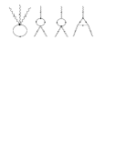
Fig. 2: Topologically inequivalent diagrams contributing to $\Gamma^{(1)\mu\nu\rho}_{(3,0)}[p_{1},p_{2},-p_{1}-p_{2}]_{\rm pole}^{\rm one-loop}$.

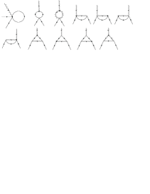
Fig. 3: Topologically inequivalent diagrams contributing to $\Gamma^{(1)\mu}_{(1,1)}[p_{1}-p_{2};p_{1},p_{2}]_{\rm pole}^{\rm one-loop}$.

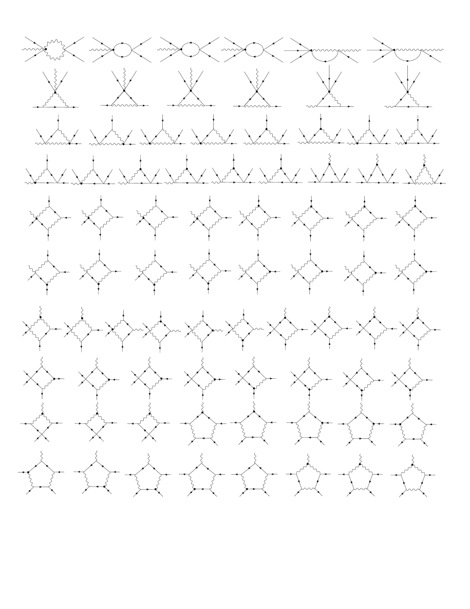
Fig. 4: Topologically inequivalent diagrams contributing to $\Gamma^{(1)\mu}_{(1,2)}[t;p,q;r,s]_{\rm pole}^{\rm one-loop}$.

$$\leftrightarrow G^{\mu\nu}[k]$$

$$\leftrightarrow G_{1}[k]$$

$$\leftrightarrow G_{2}[k]$$

$$\leftrightarrow G[k]$$

$$\leftrightarrow\tilde{\Gamma}^{t(0)\,\mu}_{(1,1,1,0)}[r;p;q]$$

$$\leftrightarrow\tilde{\Gamma}^{t(0)\,\mu\nu}_{(2,1,0,0)}[r,s;q]$$

$$\leftrightarrow\tilde{\Gamma}^{t(0)}_{(0,3,0,0)}[p,q,r]$$

$$\leftrightarrow\tilde{\Gamma}^{t(0)}_{(0,1,2,0)}[p;q,r]$$

$$\leftrightarrow\tilde{\Gamma}^{t(0)}_{(0,1,0,2)}[p;q,r]$$

$$\leftrightarrow\tilde{\Gamma}^{t(0)\mu\nu}_{(2,2,0,0)}[r,s;p,q]$$

$$\leftrightarrow\tilde{\Gamma}^{t(0)\mu\nu}_{(2,0,2,0)}[r,s;p,q]$$

$$\leftrightarrow\tilde{\Gamma}^{t(0)}_{(0,4,0,0)}[p,q,r,s]$$

$$\leftrightarrow\tilde{\Gamma}^{t(0)}_{(0,0,4,0)}[p,q,r,s]$$

$$\leftrightarrow\tilde{\Gamma}^{t(0)}_{(0,2,2,0)}[p,q;r,s]$$

$$\leftrightarrow\tilde{\Gamma}^{t(1)\mu}_{(1,1,0,0)}[r;q]$$

$$\leftrightarrow\tilde{\Gamma}^{t(1)\mu}_{(1,0,1,0)}[r;q]$$

$$\leftrightarrow\tilde{\Gamma}^{t(1)\mu\nu}_{(2,0,0,0)}[r,s]$$

$$\leftrightarrow\tilde{\Gamma}^{t(1)\mu}_{(1,2,0,0)}[r;p,q]$$

$$\leftrightarrow\tilde{\Gamma}^{t(1)\mu}_{(1,0,2,0)}[r;p,q]$$

$$\leftrightarrow\tilde{\Gamma}^{t(1)\mu}_{(1,1,1,0)}[r;p;q]$$

$$\leftrightarrow\tilde{\Gamma}^{t(1)\mu\nu\eta}_{(3,0,0,0)}[p,q,r]$$

$$\leftrightarrow\tilde{\Gamma}^{t(1)\mu\nu}_{(2,1,0,0)}[r,s;q]$$

$$\leftrightarrow\tilde{\Gamma}^{t(1)\mu\nu}_{(2,0,1,0)}[r,s;q]$$

$$\leftrightarrow\tilde{\Gamma}^{t(1)\mu\nu}_{(2,2,0,0)}[r,s;p,q]$$

$$\leftrightarrow\tilde{\Gamma}^{t(1)\mu\nu}_{(2,0,2,0)}[r,s;p,q]$$

$$\leftrightarrow\tilde{\Gamma}^{t(1)\mu\nu}_{(2,1,1,0)}[r,s;q;p]$$

$$\leftrightarrow\tilde{\Gamma}^{t(1)\mu\nu\rho}_{(3,1,0,0)}[r,s,t;q]$$

$$\leftrightarrow\tilde{\Gamma}^{t(1)\mu}_{(1,3,0,0)}[s;p,q,r]$$

$$\leftrightarrow\tilde{\Gamma}^{t(1)\mu}_{(1,1,2,0)}[s;p;q,r]$$

$$\leftrightarrow\tilde{\Gamma}^{t(1)\mu\nu\rho}_{(3,2,0,0)}[r,s,t;p,q]$$

$$\leftrightarrow\tilde{\Gamma}^{t(1)\mu\nu\rho}_{(3,0,2,0)}[r,s,t;p,q]$$

$$\leftrightarrow\tilde{\Gamma}^{t(1)\mu}_{(1,4,0,0)}[t;p,q,r,s]$$

$$\leftrightarrow\tilde{\Gamma}^{t(1)\mu}_{(1,0,4,0)}[t;p,q,r,s]$$

$$\leftrightarrow\tilde{\Gamma}^{t(1)\mu}_{(1,2,2,0)}[t;p,q;r,s]$$

Fig. 5: Feynman rules for the phase with spontaneously broken symmetry

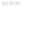
Fig. 6: Topologically inequivalent diagrams contributing to the $M-$dependent part of the gauge field two-point function.

Fig. 7: Topologically inequivalent diagrams contributing to the $M-$dependent part of the gauge field three-point function.

References

- [1] J. Madore, S. Schraml, P. Schupp and J. Wess, Eur. Phys. J. C 16 (2000) 161 [arXiv:hep-th/0001203].
- [2] B. Jurco, S. Schraml, P. Schupp and J. Wess, “Enveloping algebra valued gauge transformations for non-Abelian gauge Eur. Phys. J. C 17 (2000) 521 [arXiv:hep-th/0006246].
- [3] B. Jurco, L. Moller, S. Schraml, P. Schupp and J. Wess, Eur. Phys. J. C 21 (2001) 383 [arXiv:hep-th/0104153].
- [4] X. Calmet, B. Jurco, P. Schupp, J. Wess and M. Wohlgenannt, Eur. Phys. J. C 23 (2002) 363 [arXiv:hep-ph/0111115].
- [5] P. Aschieri, B. Jurco, P. Schupp and J. Wess, Nucl. Phys. B 651 (2003) 45 [arXiv:hep-th/0205214].
- [6] B. Melic, K. Passek-Kumericki and J. Trampetic, Phys. Rev. D 72 (2005) 054004 [arXiv:hep-ph/0503133].
- [7] B. Melic, K. Passek-Kumericki and J. Trampetic, Phys. Rev. D 72 (2005) 057502 [arXiv:hep-ph/0507231].
- [8] M. Haghighat, M. M. Ettefaghi and M. Zeinali, Phys. Rev. D 73 (2006) 013007 [arXiv:hep-ph/0511042].
- [9] M. Mohammadi Najafabadi, Phys. Rev. D 74 (2006) 025021 [arXiv:hep-ph/0606017].
- [10] A. Alboteanu, T. Ohl and R. Ruckl, Phys. Rev. D 74 (2006) 096004 [arXiv:hep-ph/0608155].
- [11] M. Buric, D. Latas, V. Radovanovic and J. Trampetic, arXiv:hep-ph/0611299.
- [12] M. Chaichian, P. Presnajder, M. M. Sheikh-Jabbari and A. Tureanu, Eur. Phys. J. C 29 (2003) 413 [arXiv:hep-th/0107055].
- [13] V. V. Khoze and J. Levell, JHEP 0409 (2004) 019 [arXiv:hep-th/0406178].
- [14] S. A. Abel, J. Jaeckel, V. V. Khoze and A. Ringwald, JHEP 0601 (2006) 105 [arXiv:hep-ph/0511197].
- [15] M. Arai, S. Saxell and A. Tureanu, arXiv:hep-th/0609198.
- [16] A. Bichl, J. Grimstrup, H. Grosse, L. Popp, M. Schweda and R. Wulkenhaar, JHEP 0106 (2001) 013 [arXiv:hep-th/0104097].
- [17] R. Wulkenhaar, JHEP 0203 (2002) 024 [arXiv:hep-th/0112248].
- [18] M. Buric and V. Radovanovic, JHEP 0210 (2002) 074 [arXiv:hep-th/0208204].
- [19] M. Buric and V. Radovanovic, JHEP 0402 (2004) 040 [arXiv:hep-th/0401103].
- [20] M. Buric, D. Latas and V. Radovanovic, JHEP 0602 (2006) 046 [arXiv:hep-th/0510133].
- [21] M. Buric, V. Radovanovic and J. Trampetic, arXiv:hep-th/0609073.
- [22] X. Calmet, arXiv:hep-th/0604030.
- [23] F. J. Petriello, Nucl. Phys. B 601 (2001) 169 [arXiv:hep-th/0101109].
- [24] B. A. Campbell and K. Kaminsky, Nucl. Phys. B 581 (2000) 240 [arXiv:hep-th/0003137].
- [25] Y. Liao, JHEP 0111 (2001) 067 [arXiv:hep-th/0110112].
- [26] Y. Liao, JHEP 0204 (2002) 042 [arXiv:hep-th/0201135].
- [27] F. Ruiz Ruiz, Nucl. Phys. B 637 (2002) 143 [arXiv:hep-th/0202011].
- [28] S. Wolfram, Mathematica, A System for Doing Mathematics by Computer (Addison-Wesley, New-York, 1991).
- [29] J. Kubo, K. Sibold and W. Zimmermann, Phys. Lett. B 220 (1989) 191.
- [30] T. Appelquist, J. Carazzone, T. Goldman and H. R. Quinn, Phys. Rev. D 8 (1973) 1747 [Phys. Rev. D 6 (1973) 1747].
- [31] M. Vargas and J. L. Lucio, “One loop renormalization of the Abelian Higgs model,” In *Oaxtepec 1990, Proceedings, Particles and fields* 485-502.