Quantisation of Parameters and the String Landscape Problem

Abstract

We broaden the domain of application of Brustein and de Alwis recent paper Brustein:2005yn , where they introduce a (dynamical) selection principle on the landscape of string solutions using FRW quantum cosmology. More precisely, we (i) explain how their analysis is based in choosing a restrictive range of parameters, thereby affecting the validity of the predictions extracted and (ii) subsequently provide a wider and cohesive description, regarding the probability distribution induced by quantum cosmological transition amplitudes. In addition, employing DeWitt’s argument DeWitt1 for an initial condition on the wave function of the Universe, we found that the string and gravitational parameters become related through interesting expressions involving an integer $n$, suggesting a quantisation relation for some of the involved parameters.

I Introduction

The existence of a multiverse of vast solutions Bousso:2000xa ; Douglas:2003um ; Susskind:2003kw to string theory Polchinski2:1998rr constitutes currently an important challenge Polchinski:2006gy : How to select a Universe or a class from the multiverse that will bear significant similarities to ours?

The framework of quantum cosmology Vilenkin:1983xq ; Hartle:1983ai ; Linde:1983cm provides a methodology to establish a probability distribution for the dynamical parameters of the universe. This distribution probability depends on the boundary condition chosen for the wave function of the Universe Hawking:1984hk ; Vilenkin:1984wp ; Linde . Extending the procedure towards string theory requires the inclusion of the dynamics of the moduli (namely, their eventual stabilisation through, e.g., fluxes and non-perturbative effects Giddings:2001yu ; Kachru:2003aw ; Douglas:2006es ). A simple setting where this quantum cosmological approach can be tested is that for which the moduli, the dilaton $S$, and the volume modulus $T$ are fixed by stringy effects (cf. ref. Brustein:2005yn ).

Recently, R. Brustein and S. P. de Alwis (BA) proposed in Brustein:2005yn , using FRW quantum cosmology, a dynamical selection principle on the landscape of string solutions Susskind:2003kw , without reference to the anthropic principle Vilenkin:2004fj ; Weinberg:2005fh . In more detail, this selection principle employs a thermal boundary condition for the wave function of the Universe and leads to results similar to those found by Sarangi and Tye Sarangi:2005cs . This boundary condition states that the Universe emerges from the string era in a thermally excited state above the Hartle-Hawking (HH) vacuum, allowing to determine a tunnelling probability to different points in the landscape. Furthermore, this primordial thermal bath is effectively described by a radiation fluid which “depends” on the cosmological constant. Moreover, these ansätze imply a switch in the usual features of the HH Hartle:1983ai and the tunnelling (Vilenkin) Vilenkin:1983xq ; Vilenkin:1998rp (see also Linde:1983cm ; Linde for a variation) wave functions: The HH wave function, once the thermal boundary condition of Brustein:2005yn is assumed, favours a non-vanishing cosmological constant larger than the one preferred by the tunnelling (Vilenkin) wave function. The extension to a model with dynamical moduli was also presented in Brustein:2005yn , applying it, e.g., to the model of Kachru, Kallosh, Linde and Trivedi (KKLT) Kachru:2003aw . BA subsequently selected a class of values for the parameters that characterise a multiverse in the landscape Brustein:2005yn .

Such a quantum cosmological scenario constitutes indeed an interesting and promising framework to address the string landscape problem. Nevertheless, there are a few significant points that do require additional investigation and which we address in this paper as follows.

In Section II we will review critically the issue of determining transition tunnelling amplitudes for a closed FRW Universe with a positive cosmological constant, $\Lambda$, and a radiation fluid (i.e., the simpler background introduced by BA in Brustein:2005yn ; Note that a detailed description of a FRW minisuperspace with a cosmological constant and a radiation fluid can be found in Halliwell:1989ky ; Bouhmadi-Lopez:2002qz ). In Section III, we thoroughly analyse the thermal boundary condition proposed in Brustein:2005yn , clarifying the approximations used therein and the limits of their applicability. In particular, we discuss how making the amount of radiation to “depend” in a very particular way on the cosmological constant is the key of BA new insight (see Eq. (15)), thereby switching the roles of the Hartle-Hawking Hartle:1983ai and tunnelling (Vilenkin) Vilenkin:1983xq ; Vilenkin:1998rp wave functions in the sense we have previously mentioned. Moreover, we prove that the thermal boundary condition applied in Brustein:2005yn corresponds to the particular physical situation where the amount of radiation is very large. Section IV constitutes an important element of our analysis. Therein, we explain how the BA analysis is based on a narrow approximation range and not fully sustainable. We then provide a broader and improved analysis that is independent of such restrictive limit; i.e. we consider an arbitrary amount of radiation consistent with the tunnelling of a radiation-filled Universe with a positive $\Lambda$. Furthermore, we point out that the switching of the roles of the Hartle-Hawking Hartle:1983ai and tunnelling (Vilenkin) Vilenkin:1983xq wave functions is not mandatory, when investigating the probability of tunnelling to different points in the landscape, under the presence of a radiation term which depends on the cosmological constant.

The FRW minisuperspace employed in the previous Sections allows to extract additional new results that were not the focus of interest in Brustein:2005yn . In fact, in Section V, we explain how a quantum mechanical formulation allows to determine how some parameters, which may characterise a multiverse in the landscape, would be related through an integer. This result is obtained by imposing DeWitt’s condition DeWitt1 ; Davidson:1999fb ; Bouhmadi-Lopez:2004mp ; i.e. the wave function vanishes at a classical singularity, to address the presence of a divergence in the curvature. More precisely, the employed FRW minisuperspace (cf. Brustein:2005yn ) has such a divergence in a classically allowed region. This singularity can be dealt with, not by replacing it with an Euclidean conic-singularity-free pole, but instead, by making it quantum mechanically inaccessible DeWitt1 ; Davidson:1999fb ; Bouhmadi-Lopez:2004mp , therefore turning it neutralised. In Section VI, we include moduli fields similarly to Brustein:2005yn , but adapting in a consistent manner the improved thermal boundary condition treatment of Section 4 towards a KKLT-like setting. Finally, in Section VII we present a summary of our work, discussing the physical implications of our results.

For completeness, let us point out the relation between the notation used in Brustein:2005yn and the followed in this paper ($\sigma^{2}=2\textrm{G}/(3\pi)$):

Our notation	BA notation
$\lambda$	$\sigma^{-2}\lambda$
$\tilde{K}$	$\sigma^{2}K$
$\nu$	$\sigma^{-2}\nu$
$a^{2}$	$\sigma^{2}a^{2}$
$t$ time	$\sigma t$
$\rho$	$\frac{1}{4\pi^{2}}\rho$
$C$	$\frac{1}{4\pi^{2}}C$
$b^{4}$	$4\pi^{2}c^{4}$
$I$	$\Phi$

II FRW Transition Amplitudes with Radiation and a positive Cosmological Constant

The aim of this section is to review (cf. Refs. Vilenkin:1998rp ; Halliwell:1989ky ; Bouhmadi-Lopez:2002qz ; Rubakov:1984bh ) the standard framework concerning transition amplitudes for a closed radiation-filled FRW Universe with a cosmological constant and for two well-known boundary conditions: the Hartle-Hawking (HH) Hartle:1983ai and tunnelling (Vilenkin) Vilenkin:1983xq .

The Wheeler-DeWitt equation for a closed FRW Universe filled with radiation, represented by a perfect fluid whose energy density is given by $\rho=3\tilde{K}/(8\pi\textrm{G}a^{4})$, and a positive cosmological constant, $\Lambda$ ($\Lambda\equiv 3\lambda$), reads

$$\left[-\frac{\textrm{G}}{3\pi}\frac{d^{2}}{d\,a^{2}}+\frac{3\pi}{4\textrm{G}}V(a)\right]\Psi(a)=0,$$ (1)

$$V(a)=a^{2}-\lambda a^{4}-\tilde{K}.$$

In the previous equations $a$ is the scale factor, G is the gravitational constant and $\tilde{K}$ is a parameter that measures the amount of radiation. It can be seen that there are two turning points $a_{\pm}$ for $0<4\tilde{K}\lambda<1$, where the potential $V$ vanishes (see Fig. 1):

$$a^{2}_{\pm}=\frac{1\pm{m}}{2\lambda},\quad m=\sqrt{1-4\tilde{K}\lambda}.$$ (2)

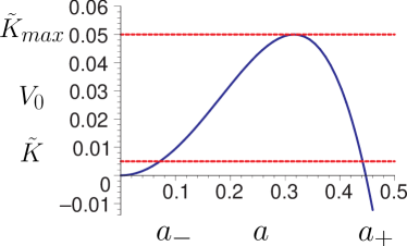
Figure 1: The blue solid line represents the potential $V_{0}$ defined as $V(a)$ given in Eq. (1) in absence of radiation; i.e. for $\tilde{K}=0$. The red dashed-lines represent different amounts of radiation given by $\tilde{K}$ and $\tilde{K}_{max}$. The turning points, $a_{\pm}$, are the solutions of $V_{0}(a)=\tilde{K}$. The larger is the amount of radiation; i.e. the larger is $\tilde{K}$, the closer are the turning points. For $\tilde{K}=\tilde{K}_{max}$, $a_{+}$ and $a_{-}$ coincide. This amount of radiation represents the border line between having a tunnelling effect and no tunnelling effect. We will refer to a Universe with an amount of radiation such that $\tilde{K}$ is close to $\tilde{K}_{max}$ (but still smaller than $\tilde{K}_{max}$) as a Universe filled with a large amount of radiation.

These turning points split the Lorentzian and Euclidean regions. We also note that the maximum of the potential $V$ is reached at

$$a_{max}\equiv a_{*}=\sqrt{1/2\lambda},$$ (3)

where

$$V(a_{*})=\frac{1}{4\lambda}-\tilde{K}.$$ (4)

Therefore, there will be always an Euclidean region as long as the condition

$$V(a_{*})>0\Leftrightarrow 4\lambda\tilde{K}<1$$ (5)

holds. Consequently, the maximum amount of radiation consistent with the tunnelling of the Universe is such that $\tilde{K}<\tilde{K}_{max}$ (see Fig. 1), where

$$\tilde{K}_{max}\equiv\frac{1}{4\lambda}.$$ (6)

From now on, for a given positive cosmological constant, we will refer to a Universe as filled with a large amount of radiation if the radiation energy density is such that $\tilde{K}$ is close to $\tilde{K}_{max}$ but still smaller than $\tilde{K}_{max}$ (see Fig. 1).

The transition amplitude, $\mathcal{A}$, of the Universe to evolve from the first Lorentzian region ($a<a_{-}$) to the larger Lorentzian region ($a>a_{+}$) can be estimated within a WKB formulation. It will depend crucially on the boundary condition imposed on the wave function of the Universe. Indeed, it is known that Vilenkin:1998rp ; Bouhmadi-Lopez:2002qz (see also Bouhmadi-Lopez:2004mp )

$$\mathcal{A}=\exp(\epsilon 2I),\quad I=\frac{3\pi}{2\textrm{G}}\int_{a_{-}}^{a_{+}}\sqrt{V(a)}\,da,$$ (7)

where $\epsilon=1$ for the HH wave function and $\epsilon=-1$ for the tunnelling (Vilenkin) wave function. Then, the transition amplitude is found as Vilenkin:1998rp ; Bouhmadi-Lopez:2002qz

$$\mathcal{A}=\exp(\epsilon 2I),\quad I=\frac{\pi}{2^{\frac{3}{2}}\textrm{G}}\tilde{K}f,$$ (8)

where

$$f=\frac{\sqrt{1+m}}{\tilde{K}\lambda}\left[\textrm{E}(\alpha_{II})-(1-m)\textrm{K}(\alpha_{II})\right],\,\,\alpha_{II}=\sqrt{\frac{2m}{1+m}},$$

(9)

with $K(m)$ and $E(m)$ as complete elliptic integrals of the first and second kind, respectively Gradshteyn .

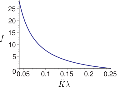
Figure 2: Plot of $f$ defined in Eq. (9) as a function of $\tilde{K}\lambda$, where $f=\epsilon\sqrt{2}\textrm{G}/(\pi\tilde{K})\ln\mathcal{A}$. For a given arbitrary amount of radiation (a given $\tilde{K}\neq 0$), the preferred value for the cosmological constant by the tunnelling (Vilenkin) boundary condition (i.e., $\epsilon=-1$) minimises $f$. On the other hand, the preferred value for the cosmological constant by the Hartle-Hawking boundary condition, (i.e., $\epsilon=1$) maximises $f$.

For a given amount of radiation; i.e. a fixed non-zero value of $\tilde{K}$, $f$ is a decreasing function of $x\equiv\tilde{K}\lambda$ (see Fig. 2). Consequently, the HH wave function suggests a vanishing cosmological constant (see Figs. 2 and 3); i.e. the largest amplitude is obtained for $x=\tilde{K}\lambda\rightarrow 0$ or $\lambda\rightarrow 0$. This is a rather curious aspect. In fact, for $\lambda\rightarrow 0$, we have $a_{+}\rightarrow\infty,~{}a_{*}\rightarrow\infty,~{}V(a_{*})\rightarrow\infty$ as $V(a)\rightarrow a^{2}-\tilde{K}$: It is an effective harmonic oscillator behaviour for a zero energy state, as the height of $V$ increases to infinity and a tunnelling endpoint goes to infinity as well. Hence, “where” does the quantum Universe tunnels to in the case of $\lambda\rightarrow 0$? On the other hand, the tunnelling (Vilenkin) wave function indicates that the largest amplitude is obtained for $x\rightarrow 1/4$; i.e. a cosmological constant such that $\tilde{K}\lambda\rightarrow 1/4$, where both turning points coincide and consequently there is no tunnelling (see Figs. 2 and 4). In addition, the maximum of the potential $V(a)$ also decreases to zero as shown in Fig. 1. In essence, there is “no potential” to tunnel from and the evolution will not correspond to a quantum mechanical transition Rubakov:1984bh .

The above asymptotic features are based on an arbitrary amount of radiation as long as $0<x<1/4$. If one considers instead a small amount of radiation such that $x=\tilde{K}\lambda\ll 1$, then $a_{+}^{2}\sim 1/\lambda$, $a_{-}\sim\tilde{K}$ and $V(a_{*})\sim 1/(4\lambda)$. Therefore, it can be easily seen that

$$f\sim\frac{\sqrt{2}}{\tilde{K}\lambda}\left[1-\frac{3}{4}\left(4\ln 2-\ln(\tilde{K}\lambda)+1\right)\tilde{K}\lambda\right],$$ (10)

for $\tilde{K}\lambda\ll 1$. Then using Eq. (8), it turns out

$$\mathcal{A}\sim\exp\left\{\left(\epsilon\frac{\Pi}{G\lambda}\right)\left[1-\frac{3}{4}\left(4\ln 2-\ln(\tilde{K}\lambda)+1\right)\tilde{K}\lambda\right]\right\}.$$

(11)

Consequently, the Vilenkin wave function is in agreement with the tunnelling of the Universe and suggests a non vanishing cosmological constant. In contrast, the HH wave function will still favour a vanishing cosmological constant: This constitutes the standard result (cf. for example refs. Vilenkin:1998rp ; Bouhmadi-Lopez:2002qz ; Rubakov:1984bh ) for the transition amplitude of a closed FRW Universe filled with a positive vacuum energy density modulated by some corrections due to the presence of a small amount of radiation in the Universe. Regarding these results, it should be added that, (i) in order to retrieve a proper tunnelling effect from the Vilenkin wave function with radiation, one needs an upper “cut off” in $\tilde{K}\lambda$ (see Figs. 2 and 4), (ii) in order to predict a non vanishing cosmological from the HH wave function one needs a lower “cut off” in $\tilde{K}\lambda$ (see Figs. 2 and 3). The inclusion in this analysis of back-reaction effects due to metric fluctuations and quantum effects due to vacuum energy, constitute recently addressed issues (see, e.g., Sarangi:2005cs ; Barvinsky:2006uh ).

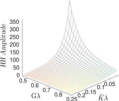
Figure 3: Plot of the transition amplitude, $\mathcal{A}$, for the HH boundary condition as a function of $x=\tilde{K}_{a}\lambda_{a}=\tilde{K}\lambda$ and $\lambda_{a}$, where $\tilde{K}_{a}$, $\lambda_{a}$ are dimensionless variables defined as $\tilde{K}_{a}=\tilde{K}/\textrm{G}$ and $\lambda_{a}=\textrm{G}\lambda$.

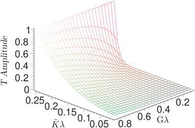
Figure 4: Plot of the transition amplitude, $\mathcal{A}$, for the tunnelling (Vilenkin) boundary condition as a function of $x=\tilde{K}_{a}\lambda_{a}=\tilde{K}\lambda$ and $\lambda_{a}$, where $\tilde{K}_{a}$, $\lambda_{a}$ are dimensionless variables defined as $\tilde{K}_{a}=\tilde{K}/\textrm{G}$ and $\lambda_{a}=\textrm{G}\lambda$.

In the next section, we describe how the presence of radiation can be employed (cf. Brustein:2005yn ) to formulate (within string theory) an initial quantum state for the universe.

III Brustein and Alwis Thermal boundary condition

Brustein and de Alwis (BA) have proposed a variant boundary condition for the wave function of the Universe Brustein:2005yn : The Universe emerges from the string era in a thermal state above the HH vacuum state (where the HH vacuum state is the HH wave function with $\tilde{K}=0$). In addition, self-consistency of their approach requires that the highest energy density on the region of interest ($a_{-}<a<a_{+}$) is such that

$$\rho(a_{-})=CM_{s}^{4}<M_{s}^{4}.$$ (12)

Therefore, the parameter $C$ satisfies $C<1$. On the other hand, BA consider that $C$ is related to the number of degrees of freedom, $n_{dof}$, in thermal equilibrium through

$$C=\frac{n_{dof}}{b^{4}}.$$ (13)

As described in Ref. Sarangi:2005cs (cf. Eq. (1.10) therein; see also Eqs. (1.2), (1.3) and (2.14) in Firouzjahi:2004mx ; also briefly pointed out in BA’s paper), $n_{dof}$ constitutes the number of light degrees of freedom included in the environment (e.g., for just pure gravity we have $n_{dof}=2$ for the two tensor modes). More precisely, the framework from which the setting in Sarangi:2005cs and consequently that of Brustein:2005yn , is retrieved is that of a (sub)system (with very limited degrees of freedom; e.g., a time dependent scale factor and a scalar field), with the remaining degrees of freedom (e.g., fluctuations of those fields) constituting the environment (which can be integrated over). Tracing over the fluctuations produces a decoherence term (cf. Ref. Claus ) which will depend on a specific cut-off. In string theory, this will depend on the (open and closed) string spectrum and has to be calculated for each vacuum, hence depending possibly on compactification and dilaton moduli, among other more complex possibilities Sarangi:2005cs ; Firouzjahi:2004mx . The inclusion and full treatment of all these features in computation of transition amplitudes can be challenging as pointed out in Ref. Firouzjahi:2004mx .

In attempting to include a parameter that would represent a string density of states, this is found to be dependent on the specific model. For example in Frey:2005jk , it is given the density of state for open strings in the context of D3 branes in Eq.(D2) and for closed strings in Eq.(D5) (see also Eqs. (1)-(2) of Ref. Abel:2002rs ). On the other hand, in Ref. Brandenberger:1988aj another expression is given for the density of state of strings compactified in a nine-dimensional box (see for example Eq.(A.1) of the mentioned paper).

For simplicity, we follow the indications and procedure in Brustein:2005yn , which adapts from Sarangi:2005cs ; Firouzjahi:2004mx .

BA approximate the smaller turning point by

$$a_{-}^{2}\thicksim\frac{1}{2\lambda}.$$ (14)

We would like to point out that this approximation is valid as long as $4\tilde{K}\lambda\simeq 1^{-}$ (following the notation introduced in Section II); i.e. the thermal effect corresponds to a large amount of radiation where $\tilde{K}$ is close to $\tilde{K}_{max}$ (see Fig. 1). Moreover, it should be noted that $4\tilde{K}\lambda\simeq 1^{-}$ implies $m\simeq 0$ leading to a potential with a very small positive height and $a_{-}\simeq a_{+}$ (cf. Eq. (2)).

Then, combining the last equations, i.e.,

• Requiring the restriction of $4\tilde{K}\lambda\simeq 1^{-}$ (or equivalently $\tilde{K}\simeq\tilde{K}_{max}$, see Fig. 1) which leads to $a_{-}^{2}\sim a_{+}^{2}\simeq 1/2\lambda$,

• Imposing subsequently the bound (12),

• Employing (13),

BA obtain

$$\rho = \frac{3\tilde{K}}{8\pi\textrm{G}}\frac{1}{a^{4}},\quad\tilde{K}\simeq\frac{\nu}{\lambda^{2}},$$ (15)

$$\nu \equiv \frac{2}{3}n_{dof}b^{-4}\pi\textrm{G}M_{s}^{4}.$$

In this manner, the radiation term “depends” explicitly on the cosmological constant $\lambda$.

On the one hand, BA then conclude that the HH wave function in this case favours a positive non-vanishing cosmological constant Brustein:2005yn , differently to what is exposed in Section II. The reason these authors got a different answer is because they asked a different question. Let us be more precise: Instead of looking for values of $\lambda$ that maximise the transition amplitude for a fixed value of $\tilde{K}$, they looked for values of $\lambda$ that maximise the transition amplitude for a fixed value of $\nu$. Indeed, the transition amplitude, $\mathcal{A}$, can be rewritten as

$$\mathcal{A}=\exp(\epsilon 2I),\quad I=\frac{\pi}{2^{\frac{3}{2}}\textrm{G}}\frac{1}{\nu}g,$$ (16)

where

$$g=\frac{\nu}{\lambda}{\sqrt{1+m}}\left[\textrm{E}(\alpha_{II})-(1-m)\textrm{K}(\alpha_{II})\right],\,\,\alpha_{II}=\sqrt{\frac{2m}{1+m}}.$$

(17)

Then, it can be seen that the function $g$ is an increasing function of $\nu/\lambda$ until the ratio $\nu/\lambda$ approaches $0.12$ and then it starts decreasing (see Fig. 5). Consequently, for a fixed value of $\nu$ the HH wave function favours a non-vanishing cosmological constant, namely $\lambda\simeq\ 8.33\,\nu$.

However, let us point out that the result $\lambda\simeq\ 8.33\,\nu$ is not quite compatible with the approximation claimed by BA in Brustein:2005yn (see Eq. (14)); i.e. $\lambda\simeq\ 4\,\nu$. Moreover, the use of a WKB approximation is valid as long as

$$\rm{G}\left|\frac{dV(a)}{da}\right|\ll{\left|V(a)\right|}^{3/2}.$$ (18)

So, if $4\tilde{K}\lambda\simeq 1^{-}$, the scale factor in the Euclidean region will be of the order of $a_{-}$ or $a_{+}$; i.e. of the order of $1/\sqrt{2\lambda}$ (cf. Eq. (14) and the paragraph below). Consequently, the WKB approximation breaks down below the barrier because both sides of the inequality (18) vanish. In more detail, the WKB approximation can still hold in the Lorentzian regions but not in the Euclidean region. Nevertheless this weakness can be dealt with. In fact, we will provide in Section IV a broader and improved analysis for the thermal boundary condition without the restriction $4\tilde{K}\lambda\simeq 1^{-}$. We will also show how some of the conclusions reached in Brustein:2005yn can be reversed.

On the other hand, the tunnelling (Vilenkin) wave function modified by the thermal effects and for a fixed value of $\nu$, either favours (i) $\nu/\lambda\rightarrow 0$ (large $\lambda$ and small $\tilde{K}$) which is incompatible with the approximation assumed in Brustein:2005yn (cf. Eq. (14)) or favours (ii) no tunnelling, since $\lambda\simeq\ 4\,\nu$ (or equivalently $4\tilde{K}\lambda\simeq\ 1$). These features are shown in Fig. 5.

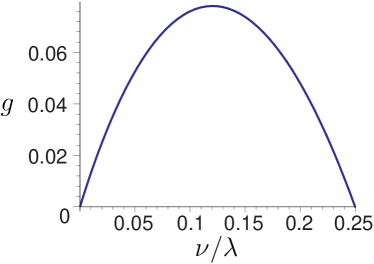
Figure 5: Plot of $g$ defined in Eq. (17) as a function of $\nu/\lambda$, where $g=\epsilon\frac{\sqrt{2}}{\pi}\textrm{G}\,\nu\ln\mathcal{A}$. For a given arbitrary $\nu$, the preferred value for the cosmological constant by the tunnelling (Vilenkin) boundary condition (i.e. $\epsilon=-1$) minimises $g$. On the other hand, the preferred value for the cosmological constant by the HH boundary condition, (i.e. $\epsilon=1$) maximises $g$.

IV A Broader Analysis of the Brustein-Alwis Boundary Condition

In this section, we (i) widen and improve the application of the thermal boundary condition Brustein:2005yn and (ii) will see how some of the results obtained in the previous section are then modified when we relax the condition $4\tilde{K}\lambda\simeq 1^{-}$ (implicitly assumed in Brustein:2005yn ). We designate the broader setting introduced in this section as generalised thermal boundary condition for the wave function. Herein:

• We will assume instead an arbitrary amount of radiation, consistent with a tunnelling of the Universe; i.e. $\tilde{K}<\tilde{K}_{max}$ (see Fig. 1);

• We will not assume the approximation used in Eq. (14) and therefore we will rather consider the full expression (2) for $a_{-}$ given in Section II;

• Consequently, we will not restrict ourselves to the particular situation corresponding to a large amount of radiation;

• The radiation energy density still reads

  $$\rho=\frac{3\tilde{K}}{8\pi\textrm{G}}\frac{1}{a^{4}},$$ (19)

  but now $\tilde{K}$ is related to the cosmological constant through the more general expression

  $$\tilde{K}=\frac{4\nu\lambda^{-2}}{(1+4\nu\lambda^{-1})^{2}},$$ (20)

  while $\nu$ is defined as before; i.e.

  $$\nu\equiv\frac{2}{3}n_{dof}b^{-4}\pi\textrm{G}M_{s}^{4}.$$ (21)

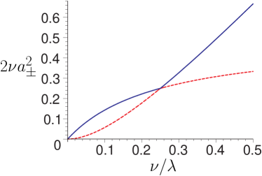
Figure 6: Plot of the dimensionless turning points $2\nu a^{2}_{\pm}$ as a function of $\nu/\lambda$. The blue solid line corresponds to the larger turning point $2\nu a^{2}_{+}$. The red dash-dot line corresponds to the smaller turning point $2\nu a^{2}_{-}$. Although it seems that both turning points coincide for very small values of $\nu/\lambda$ it is not the case (see the text). Consequently, even in this case the Universe can tunnel through the barrier $V(a)$. For $\nu/\lambda$ approaching $1/4$ both turning points coincides and consequently there is no tunnelling.

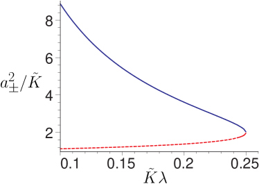
Figure 7: Plot of the dimensionless turning points $a^{2}_{\pm}/\tilde{K}$ as a function of $\tilde{K}\lambda$. The blue solid line corresponds to the large turning point $a^{2}_{+}/\tilde{K}$. The red dash-dot line corresponds to the smaller turning point $a^{2}_{-}/\tilde{K}$. For $\tilde{K}\lambda$ approaching $1/4$ both turning points coincide and there is no tunnelling.

It should hence be noticed that we recover Eq. (15) using Eqs. (19)-(21) when $4\nu/\lambda$ is approaching 1. In this limit, both turning points come closer. Indeed, $a_{-}$ and $a_{+}$ coincide at $4\nu/\lambda=1$ (see Fig. 6). Equivalently, in this case $4\tilde{K}\lambda$ is approaching 1 being the case where both turning points overlap, inducing no tunnelling. This limiting case is represented by a square in Figs. 8 and 9 (see also Fig. 7).

From Fig. 6, it looks like that there is another physical situation where both turning points would coincide, corresponding to a large cosmological constant ($\nu/\lambda\rightarrow 0$) and a small amount of radiation as measured by the parameter $\tilde{K}$ ($\tilde{K}\lambda\rightarrow 0$). This limiting case is represented by a circle in Figs. 8 and 9. However, in this case it can be easily seen that although the turning points are small

$$a_{-}^{2}\sim\frac{4\nu}{\lambda^{2}}\sim\tilde{K},\quad a_{+}^{2}\sim\frac{1}{\lambda},$$ (22)

their relative ratio is very large

$$\frac{a_{+}^{2}}{a_{-}^{2}}\sim\frac{1}{\tilde{K}\lambda}\gg 1.$$ (23)

Consequently, the Universe may still tunnel from the first Lorentzian region to the larger one. This comment will be important for the tunnelling (Vilenkin) proposal (see below and Fig. 9).

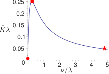
Figure 8: Plot of $\tilde{K}\lambda$ as a function of $\nu/\lambda$. $\nu/\lambda$ is bivalued as a function of $\tilde{K}\lambda$ except in the particular case $4\nu/\lambda=1$ or equivalently $4\tilde{K}\lambda=1$. There is a one to one correspondence between the circle, the square and the star in this plot and the ones in Fig. 9.

Within the broader range employed in this section, the relevant feature is that the transition amplitude as a function of $\nu/\lambda$ will be unlike the one deduced in Brustein:2005yn . This is represented in Fig. 9, which is indeed quite distinct from Fig. 5. The reason is that the dependence of the radiation energy density on $\lambda$ is modified with respect to the one used in Section III (cf. Eqs. (15) and (20)), although the transition amplitude is given by Eqs.(8) or (17). Our generalised expressions for the transition amplitudes involve the use of Eqs. (8)-(9) or Eqs. (16)-(17), but with the parameter $m$ given by

$$m=\frac{|1-4\frac{\nu}{\lambda}|}{1+4\frac{\nu}{\lambda}}.$$ (24)

and therefore the parameter $\alpha_{II}$ in Eq. (9) or Eq. (17) is modified accordingly. Moreover, the modification of the transition amplitude with respect to BA case is due to the modified Eq. (20) which is different from Eq. (15). A plot of $g$ relevant for our new generalised expressions for the transition amplitude is given in Fig. 9.

In such context, a pertinent question follows: What will be then the most likely value of the cosmological constant for a given value of $\nu$?

Regarding the HH wave function, it now favours a vanishing cosmological constant ($\nu/\lambda\rightarrow\infty$) and $\tilde{K}\sim 1/(4\nu)$. This physical case is represented schematically by a star in Figs. 8 and 9. The turning points can be approximated by

$$a_{-}^{2}\sim\frac{1}{4\nu}\sim\tilde{K},\quad a_{+}^{2}\sim\frac{1}{\lambda},$$ (25)

and, in particular, it turns out that

$$\frac{a_{+}^{2}}{a_{-}^{2}}\sim\frac{1}{\tilde{K}\lambda}\gg 1.$$ (26)

Moreover, it can be easily shown that the transition amplitude in this case can be approximated by

$$\mathcal{A} \sim \exp\left\{\frac{\pi}{\rm{G}{\lambda}}\left[1-\frac{3}{16}\left(6\ln 2-\ln\frac{\lambda}{\nu}+1\right)\frac{\lambda}{\nu}\right]\right\}$$

$$\sim \exp\left\{\frac{\pi}{\rm{G}{\lambda}}\left[1-\frac{3}{4}\left(4\ln 2-\ln(\tilde{K}{\lambda})+1\right){\tilde{K}}{\lambda}\right]\right\}.$$

In this manner, the role of the HH wave function and subsequent transition amplitude is returned to its “original” implication, with the thermal boundary condition being implemented in a fully consistent manner and not restricted to a narrow (perhaps not fully valid) limit. Notice as well that the expressions (22) [(23)] and (25) [(26)] coincide as a function of $\tilde{K}$, though they correspond to different physical situations. Indeed, the limiting case corresponding to Eqs. (22) and (23) [(25) and (26)] is represented by a circle [star] in Figs. 8 and 9. Furthermore, even though the maximum height of the potential in both cases is given by the same expression $V(a_{*})\sim 1/(4\lambda)$, in the HH case $V(a_{*})$ is very large because $\lambda$ is very small, while in the other case, depicted by a “circle” in Figs. 8 and 9, the height of the potential is very small because $\lambda$ is very large. In addition, it turns out that in both cases after the tunnelling, the size of the Universe does not depend on $\nu$ or on the number of “degrees of freedom”, although the maximum size of the first Lorentzian region depends on $\nu$. The expressions (22) [(23)] and (25) [(26)] coincide when taken as a function of $\tilde{K}$, because $\nu/\lambda$ is bivalued as a function of $\tilde{K}\lambda$ (except in the particular case $4\nu/\lambda=1$ or equivalently $4\tilde{K}\lambda=1$) (cf. Fig. 8).

Concerning the tunnelling (Vilenkin) wave function, it favours two possible physical situations depicted by a circle and a square in Figs. 8 and 9. On the one hand, the “circle” option corresponds to a large cosmological constant ($\nu/\lambda\rightarrow 0$) and a small amount of radiation as measured by $\tilde{K}$ ($\tilde{K}\lambda\rightarrow 0$), with the turning points being given in Eq. (22) and where the transition amplitude can be approximated by

$$\mathcal{A} \sim \exp\left\{-\frac{\pi}{\rm{G}{\lambda}}\left[1-{3}\left(2\ln 2-\ln\frac{\nu}{\lambda}+1\right)\frac{\nu}{\lambda}\right]\right\}$$

$$\sim \exp\left\{-\frac{\pi}{\rm{G}{\lambda}}\left[1-\frac{3}{4}\left(4\ln 2-\ln(\tilde{K}{\lambda})+1\right){\tilde{K}}{\lambda}\right]\right\}.$$

On the other hand, the “square” option implies no tunnelling, that is, $4\nu/\lambda\rightarrow 1$ or equivalently $4\tilde{K}\lambda\rightarrow 1$; i.e. both turning points coincide. In this case, the transition amplitude can be written as

$$\mathcal{A} \sim \exp\left[-\frac{3\pi^{2}}{32\sqrt{2}}\frac{1}{\rm{G}\lambda}\left(1-4\frac{\nu}{\lambda}\right)^{2}\right]$$ (29)

$$\sim \exp\left[-\frac{3\pi^{2}}{32\sqrt{2}}\frac{1}{\rm{G}\lambda}\left(1-4\tilde{K}{\lambda}\right)^{2}\right].$$

It is not possible at this stage to indicate which of these two possibilities is more likely. In order to shed some light on this question, we will employ DeWitt’s argument DeWitt1 ; Davidson:1999fb ; Bouhmadi-Lopez:2004mp in Section V.

Before proceeding, let us clarify the following concerning our results in this section:

• Eq. (22) (corresponding to a circle in Figs. 8 and 9) corresponds to the turning points for small amount of radiation as measured by $\tilde{K}$ and a large $\lambda$. The transition amplitude in this limiting case is given in Eq. (LABEL:amplitude3). This means we discussed the case with radiation density being less than the amount which saturates the limit for semiclassical consistency (cf. Ref. Brustein:2005yn ).

• The amount of radiation can be made smaller than the above (with respect to $M_{s}^{4}$), by having a smaller constant $C$. But this situation does not change our results significantly.

• Eq. (25) (corresponding to a star in Figs. 8 and 9) corresponds to the turning points for $\nu/\lambda\rightarrow\infty$; i.e. a small cosmological constant and $\tilde{K}\sim 1/(4\nu)$. The last condition comes from taking the limit $\nu/\lambda\rightarrow\infty$ in Eq. (20). The transition amplitude in this limiting case is given in Eq. (LABEL:amplitude2).

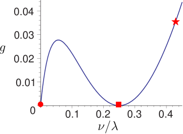
Figure 9: Plot of $g$ introduced in Eq. (17) with the parameter $m$ given in Eq. (24) as a function of the ratio $\nu/\lambda$. There is a one to one correspondence between the circle, the square and the star in this plot and the ones in Fig. 8. The preferred cosmological situation by the HH wave function is depicted by a star in the plot. The preferred cosmological situations by the tunnelling (Vilenkin) wave function is depicted by a circle and a square in the figure.

When the radiation density exceeds the semiclassical saturation bound, specific string effects would have to be considered Frey:2005jk ; Abel:2002rs ; Brandenberger:1988aj ; Leblanc:1988eq ; Lee:1997iz .

In the heterotic string theory Leblanc:1988eq below the Hagedorn temperature essentially only the massless excitations (radiation) contribute to the energy density of the gas of the heterotic string excitations. As one approaches the Hagedorn temperatures i) the radiation density gets larger and larger, meaning larger and larger values for $C$, which implies a smaller scale factor and therefore a larger temperature and ii) the energy density associated with the massive strings is no longer negligible. Therefore, the expression for the energy density that fills the universe would be radiation plus other components. A subsequent analysis will have to include the energy density of the massive states.

In a complementary context, from the thermodynamics of strings in the background of D-branes, it can be also assumed that open string dominates over closed strings Frey:2005jk ; Lee:1997iz . For example, particularising to the case of $D3$ branes, the equation of state for the open string gas in the Hagedorn regime was given in Frey:2005jk ; Abel:2002rs . This equation of state is a specific case of a generalised Chaplygin gas equation of state where the strings will redshift like dust; i.e. pressure less matter. In this case a dust term must be added to the potential $V(a)$ (see Eq. (1)) in addition to the radiation term and the cosmological constant. The gas of strings will modify the turning points. If $\tilde{K}$ acquire its maximum allowed value in absence of a gas of strings then there are no longer turning points and therefore no tunnelling. On the other hand, if $\tilde{K}$ is small enough then there are two turning points (closer than in absence of a gas of strings) and the transition amplitude given by Eq. (8) will be smaller. This conclusion is based in comparing a situation with and without a gas of strings but with the same amount of radiation, i.e. same $\tilde{K}$. However, this situation is not very realistic because the parameter $\tilde{K}$ should be smaller in presence of a gas of strings.

Of course, the transfer of energy from open strings into radiation (in the reheating phase) can be introduced. Then, the energy densities of the string gas and radiation will depend on the Hubble rate (see Ref. Frey:2005jk ) which takes into account the energy loss of strings into radiation. Now, because the energy densities depends on the Hubble rate, $H$, the Friedmann equation is different (it is cubic in $H$). This fact will modify the Hamiltonian constraint and therefore induce a modification of the Wheeler-DeWitt equation. This analysis is out of the scope of this paper. In any case, we would like to stress that in the present paper, we are interested in a situation below the Hagedorn temperature like in Ref. Brustein:2005yn .

V DeWitt’s argument and the Brustein and Alwis boundary condition

A pertinent feature concerning the minisuperspace of a closed FRW Universe with radiation and a positive cosmological constant is that a classically allowed (Lorentzian) region may exist for $0<a<a_{-}$ (cf. Fig. 1 and Eq. (2)). This is of relevance due to the following. It can be shown that for small values of the scale factor the corresponding Ricci curvature is not well defined. Indeed, it diverges. In order to deal quantum mechanically with this situation an interesting procedure was advocated by B. DeWitt DeWitt1 , which has been recently used in Refs. Davidson:1999fb ; Bouhmadi-Lopez:2004mp . In more detail, DeWitt’s argument involves the assumption that the wave function vanishes at the singularity; i.e. at $a=0$ for our FRW model.

The DeWitt’s argument applied to BA wave function yields Bouhmadi-Lopez:2004mp

$$\frac{3\pi}{2\textrm{G}}\int_{0}^{a_{-}}\,\sqrt{-V(a)}\,da-\frac{\pi}{4}=n\pi,\quad n\in\mathbb{N}.$$ (30)

The previous condition results in (see for example Bouhmadi-Lopez:2002qz )

$$\frac{\pi}{2^{\frac{3}{2}}\textrm{G}\lambda}\sqrt{1+m}\left[\textrm{E}(\alpha_{I})-m\textrm{K}(\alpha_{I})\right]-\frac{\pi}{4}=n\pi,$$ (31)

where

$$\alpha_{I}=\sqrt{\frac{1-m}{1+m}}.$$ (32)

We recall that the thermal boundary condition under the description of Ref. Brustein:2005yn (cf. Section 3) suggests $\lambda\thicksim\ 8.33\,\nu$. Consequently, we obtain

$$\textrm{G}\lambda\thicksim 0.4\sqrt{2}(1+4n)^{-1},$$ (33)

which implies not only that the weaker is gravity (smaller $G$), the larger is the cosmological constant (for a fixed value of $n$) but also that there is a quantification relation between $G$ and $\lambda$.

As we already mentioned in Section III, $\lambda\thicksim\ 8.33\,\nu$ is not fully in agreement with the approximation made in Eq. (14): $\lambda\thicksim\ 4\,\nu$, i.e. with a large amount of radiation (see Fig. 1) implicit on the BA thermal boundary condition context (see the third line before Eq. (13) in Brustein:2005yn ). If we take into account the approximation in Eq. (14) or equivalently $\lambda\thicksim\ 4\,\nu$, then it turns out that

$$\textrm{G}\lambda\thicksim\sqrt{2}(1+4n)^{-1}.$$ (34)

Consequently, we obtain a fairly similar conclusion.

Another interesting result follows for the cosmological constant and the string mass scale. In fact, Eq. (15) and the quantification relation (34) (the final result between $M_{s}$ and $\lambda$ is slightly modified for Eq. (33)) implies

$$\frac{2^{3/2}}{3}\frac{n_{dof}}{b^{4}}\pi M_{s}^{4}\thicksim\lambda^{2}\left(n+\frac{1}{4}\right).$$ (35)

The larger is $M_{s}^{2}$, the larger is $\lambda$ (for fixed values of $n$, $b$ and $n_{dof}$). In addition, the larger is $n$, the smaller is the cosmological constant (given $M_{s}^{2}$, $b$ and $n_{dof}$ fixed).

Finally, we would like to point out that the previous relations given in Eqs. (34) and (35) implies a relation between $M_{s}$, $M_{p}$ ($\textrm{G}=M_{p}^{-2}$) and $n_{dof}$:

$$M_{p}^{4}\thicksim\frac{2^{5/2}}{3}\frac{n_{dof}}{b^{4}}\pi M_{s}^{4}(1+4n).$$ (36)

It turns out that the larger is $M_{s}$, the smaller is the number of degrees of freedom in thermal equilibrium given by $n_{dof}$ (for fixed values of $n$, $b$ and $M_{p}$). This result is in agreement with Eqs. (34) and (35) under the same assumptions; i.e. for fixed values of $n$, $b$ and $M_{p}$.

Let us now apply DeWitt’s argument DeWitt1 (see also Davidson:1999fb ; Bouhmadi-Lopez:2004mp ) to establish which of the two possibilities favoured by the tunnelling wave functions (see Eqs. (LABEL:amplitude3)and (29)) is more probable once the generalised thermal boundary condition is imposed (cf. Section IV).

It is then crucial to remark the following. The modified tunnelling (Vilenkin) wave function by the thermal effect proposed in Brustein:2005yn (and assuming the approximation used in Eq.(14) which is implicit in Brustein:2005yn ) is incompatible with DeWitt’s argument. The reason is that such wave function favours no tunnelling; i.e. the turning points are of the same order of magnitude ($a_{\pm}^{2}\thicksim 1/(2\lambda)$), while DeWitt’s argument applied to the tunnelling wave function requires a “wide barrier”, more precisely Bouhmadi-Lopez:2004mp

$$1\ll\exp\left[\frac{3\pi}{2\textrm{G}}\int_{a_{-}}^{a_{+}}\sqrt{V(a)}\;da\right].$$ (37)

Consequently, if $a_{\pm}^{2}\thicksim 1/(2\lambda)$, the previous condition cannot hold and we cannot apply the DeWitt argument to the tunnelling wave function within the context of Brustein:2005yn (i.e., of Section 3), which reads Bouhmadi-Lopez:2004mp

$$\frac{3\pi}{2\textrm{G}}\int_{0}^{a_{-}}\sqrt{-V(a)}\;da=\frac{3\pi}{4}+\tilde{n}\pi,\quad\tilde{n}\in\mathbb{N};$$ (38)

or equivalently

$$\frac{\pi}{2^{\frac{3}{2}}\textrm{G}\lambda}\sqrt{1+m}\left[\textrm{E}(\alpha_{I})-m\textrm{K}(\alpha_{I})\right]-\frac{3\pi}{4}=\tilde{n}\pi,$$ (39)

where $\alpha_{I}$ is defined in Eq. (32).

However, it turns out that we can indeed apply the DeWitt’s argument to the tunnelling (Vilenkin) wave function but within the “generalised” analysis for the thermal boundary condition (cf. Section IV). The condition (37) is required to hold. So firstly, we check if this condition can be fulfilled.

Following the analysis of Section IV, it turns out that the tunnelling wave function favours either (i) a large cosmological constant ($\nu/\lambda\rightarrow 0$) and a small amount of radiation as measured by $\tilde{K}$ ($\tilde{K}\lambda\rightarrow 0$) or (ii) that there is no tunnelling, that is, $4\nu/\lambda\rightarrow 1$ which implies $4\tilde{K}\lambda\rightarrow 1$. These features are depicted in Figs. 8 and 9.

Condition (ii) is incompatible with the condition (37) because for (ii) there is no tunnelling.

Condition (i) is compatible (and therefore chosen) within the DeWitt’s requirement despite that $\nu/\lambda\rightarrow 0$ implies $g\rightarrow 0$. For $\nu/\lambda\rightarrow 0$ the function $g$ (related to the transition amplitude (defined in Eq. (17) where $m$ is given by Eq. (24)) can be approximated by

$$g\thickapprox\sqrt{2}\;\frac{\nu}{\lambda}.$$ (40)

Consequently, the condition (37) reads

$$1\ll\exp\left(\frac{\pi M_{p}^{2}}{2\lambda}\right),$$ (41)

which implies that the DeWitt argument is satisfied as long as the cosmological constant $\lambda$ is much smaller than $M_{p}^{2}$. In this case, the quantisation relation (38) reads

$$\frac{3\pi}{2}\frac{\nu}{\textrm{G}\lambda^{2}}\thicksim\frac{3}{4}+\tilde{n}.$$ (42)

Substituting the definition of $\nu$ in the previous equation results on

$$\pi^{2}\frac{n_{dof}}{b^{4}}M_{s}^{4}\thicksim\left(\frac{3}{4}+\tilde{n}\right)\lambda^{2}.$$ (43)

Consequently, the larger is $M_{s}^{2}$, the larger is $\lambda$ (for fixed values of $\tilde{n}$, $b$ and $n_{dof}$). In addition, the larger is $\tilde{n}$, the smaller is the cosmological constant (given $M_{s}^{2}$, $b$ and $n_{dof}$ fixed).

In order to get a relation between $M_{p}$, $M_{s}$ and $n_{dof}$, it is necessary to go to the next order in the expansion of Eq. (38) as a function $\nu/\lambda$.

We recall that the DeWitt’s argument is applied in the Lorentzian regions $0<a<a_{-}$ where the tunnelling (Vilenkin) wave function is a superposition of ingoing and outgoing modes. In fact, the tunnelling wave function for a closed FRW Universe filled with radiation and a positive cosmological constant in the Lorentzian region $0<a<a_{-}$ is a linear combination of ingoing and outgoing modes and not a sum of decaying and growing modes. To be more precise, from a classical point of view the region $0<a<a_{-}$ describes a Universe that starts at $a=0$ and expands up to a maximum radius $a_{-}$, as depicted in Fig. 1 of Ref. Vilenkin:1998rp . Therefore, the tunnelling wave function on this region cannot be formed from decaying and growing modes, in particular close to $a=0$, because this region does not correspond to a Euclidean region. It is in absence of radiation (which is not the physical situation analysed in this paper) that the tunnelling wave function corresponds to a sum of growing and decaying modes for $0<a<1/(2\lambda)$, in particular close to $a=0$, as is illustrated in Fig. 2 of Vilenkin:1998rp . We refer the reader to Refs. Davidson:1999fb ; Bouhmadi-Lopez:2004mp for a detailed discussion on the DeWitt’s argument, the tunnelling wave function and the Hartle-Hawking wave function.

For completeness, let us see what happens to the set of parameters once the DeWitt’s argument is imposed within HH case once the generalised thermal boundary condition is assumed. In this case $\lambda/\nu\rightarrow 0$. Using Eq. (31), where now $m$ is given by Eq. (24) and in the limiting case $\lambda/\nu\rightarrow 0$, it turns out that

$$M_{p}^{2}\sim\frac{8}{3\pi}(1+4n)\nu.$$ (44)

Furthermore, substituting the definition of $\nu$ in the previous equation results on

$$M_{p}^{4}\sim\frac{16}{9}(1+4n)\frac{n_{dof}}{b^{4}}M_{s}^{4}.$$ (45)

Notice that the previous expression is fairly similar to Eq. (36). On the other hand, notice also that the last two expressions do not depend on the cosmological constant.

VI Including Moduli Fields

Up to now, we have been using a simplified model by considering $\lambda$ constant. However, rather than a cosmological constant we expect to have a moduli dependent potential $\lambda(\phi)$. Moreover, the ratio $M_{s}^{2}/M_{p}^{2}$ will also depend on $\phi$ (c.f. Brustein:2005yn and references therein). In the heterotic string theory $M_{s}^{2}/M_{p}^{2}=\alpha_{YM}/8$, where $\alpha_{YM}$ is the gauge field coupling strength at the string scale. On the other hand, in type I string theory $M_{s}^{2}/M_{p}^{2}=g\;\alpha_{YM}/4$, where $g$ is the string coupling. Our aim in this section is to constrain (at least qualitatively) how the Universe (in the presence of moduli fields) will behave after its tunnelling. This will be presented within the broader discussion of the generalised thermal boundary condition introduced in Section IV. To be more precise, this will allow us to discuss in a more self-consistent manner the issue of transition amplitude and corresponding probability distribution, when the presence of moduli fields and their potentials is of relevance.

VI.1 “Flat” moduli potential

Let us consider a rather particular situation, namely that the moduli potential, $\bar{V}(\phi)\equiv\sigma^{2}\lambda(\phi)$, is flat enough; i.e.

$$\left|\frac{d\lambda}{d\phi}\right|\ll\left|\lambda(\phi)\right|,$$

at least just after the tunnelling of the Universe. In other words, we take the case (not likely in string theory) that the moduli potential is not steep (cf. also Brustein:2005yn ). Consequently, applying the framework introduced by Vilenkin in Vilenkin:1987kf , we can substitute $\lambda$ by $\lambda(\phi)$ in the expressions obtained previously.

Then adapting the expressions in section IV consistently, we found for the tunnelling (Vilenkin) wave function that there are two possibilities:

1. If $\lambda\sim 4\nu$ then

   $$\frac{3\pi}{2}\sigma^{2}{\lambda(\phi)}=\frac{8\pi}{3}\frac{n_{dof}}{b^{4}}\left(\frac{M_{s}}{M_{p}}\right)^{4}(\phi),$$ (46)

   where $\sigma^{2}={2\rm{G}}/(3\pi)$. By considering that $\lambda$ is much smaller than the Planck scale; i.e. $\lambda/M_{p}^{2}\ll 1$ where ${\rm{G}}=M_{p}^{-2}$ and as we are working in a semiclassical framework, we can conclude that the tunnelling (Vilenkin) wave function (once the generalised thermal boundary condition is applied) seems to favour the emergence of a weakly coupled Universe (at least in the heterotic and type I theories).

2. If $\nu/\lambda\ll 1$ then

   $$\frac{2\pi}{3}\frac{n_{dof}}{b^{4}}\left(\frac{M_{s}}{M_{p}}\right)^{4}(\phi)\ll\frac{3\pi}{2}\sigma^{2}{\lambda(\phi)}.$$ (47)

   Following the argument of the previous item, we can conclude that in this case the tunnelling (Vilenkin) wave function (once the generalised thermal boundary condition is applied) seems to favour the tunnelling of the Universe towards a weakly coupled regime.

Finally, as we have shown in Section IV, the HH wave function (once the generalised thermal boundary condition is imposed) implies $\nu/\lambda\gg 1$ and consequently:

$$\frac{2\pi}{3}\frac{n_{dof}}{b^{4}}\left(\frac{M_{s}}{M_{p}}\right)^{4}(\phi)\gg\frac{3\pi}{2}\sigma^{2}{\lambda(\phi)}.$$ (48)

Unlike for the tunnelling (Vilenkin) wave function, we cannot in principle conclude that the Universe will tunnel to a weakly coupled regime. Essentially, it is not enough to impose that $\lambda$ is much smaller than the Planck scale to “predict” the emergence of a weakly coupled Universe.

VI.2 Moduli fields and the tunnelling probability

In the previous subsection, we have supposed that (i) the moduli potential is flat enough and (ii) the potential dominates the total energy density in such a way that the tunnelling towards an inflating Universe takes place. However, it turns out that the moduli potentials are in general quite steep, leading to a dominance of the kinetic energy density of the scalar field over its potential energy Brustein:2004jp . This condition is incompatible with the emergence of an accelerating Universe. Possible exceptions correspond to the only flat regions of the moduli potentials (that support a tunnelling of the Universe towards an accelerated regime and are characterised by $\bar{V}^{\prime}/\bar{V}\ll 1$ with ${}^{\prime}\equiv d/d\phi^{i}$ and $i$ labelling the different moduli), which constitute limited domains close to a positive extremum of the potentials Brustein:2005yn . Let us consider (as in Brustein:2005yn ) a moduli potential $\bar{V}$ cast in the form of an $N=1$ SUGRA potential, where the Kähler potential involves the real part of the dilaton axion field $S_{r}$ and the real part of the volume modulus $T_{r}$. These fields determine the ratio $({M_{s}}/{M_{p}})^{4}$ as $1/(S_{r}T_{r}^{3})$ Brustein:2005yn .

The moduli $S_{r}$ and $T_{r}$ are constrained to satisfy the “flat enough” condition near an extremum

$$\bar{V}^{\prime}/\bar{V}\sim 0.$$ (49)

This condition is consistent with an accelerated expansion phase of the Universe after the tunnelling. Moreover, the maximisation of the transition amplitude of the tunnelling (Vilenkin) wave function (once the generalised thermal boundary condition is imposed) implies two possibilities, adapting the reasoning employed for Eqs. (46) and (47), respectively:

1. The moduli potential is then constrained as follows

   $$\bar{V}(S_{r},T_{r})\sim\frac{16}{9}\frac{n_{dof}}{b^{4}}\frac{1}{S_{r}T_{r}^{3}}.$$ (50)

   We would like to point out that in this particular case the extremisation condition (49) comes from imposing the emergence of an accelerating Universe and not from the tunnelling of the Universe towards an inflating Universe. We recall that in this particular case the tunnelling (Vilenkin) wave function predicts “no tunnelling”. From now on we will disregard this case.

2. The other possibility is that the moduli potential is constrained by

   $$\frac{4}{9}\frac{n_{dof}}{b^{4}}\frac{1}{S_{r}T_{r}^{3}}\ll\bar{V}(S_{r},T_{r}).$$ (51)

However, the maximisation of the transition amplitude of the HH wave function (once the generalised thermal boundary condition is imposed) implies (cf. Eq. (48))

$$\bar{V}(S_{r},T_{r})\ll\frac{4}{9}\frac{n_{dof}}{b^{4}}\frac{1}{S_{r}T_{r}^{3}}.$$ (52)

In summary, the generalised thermal boundary condition of Section IV, when applied to the wave function of the Universe, produces less restrictive conditions than the ones extracted by BA in Brustein:2005yn .

VI.3 Application to a KKLT-like model

Before concluding this section, let us apply the above discussion to a KKLT model Kachru:2003aw , where the effective moduli potential is given by Kachru:2003aw

$$\bar{V}=\frac{aCe^{-aT_{r}}}{2T_{r}^{2}}\left[W_{0}+\left(\frac{1}{3}T_{r}a+1\right)Ce^{-aT_{r}}\right]+\frac{d}{T_{r}^{3}}.$$ (53)

In this expression $a$, $C$, $W_{0}$ and $d$ are constant and the rest of moduli have been stabilised (in particular $S_{r}\sim O(1)$ Brustein:2005yn ). This potential has a positive maximum separating a positive minimum from the asymptotically vanishing potential corresponding to the tail of the potential where the term $d/T_{r}^{3}$ dominates Kachru:2003aw .

Let us see if the conditions (51) and (52) can be fulfilled at the tail of the potential. In this case these conditions read $\frac{4}{9}\frac{n_{dof}}{b^{4}}\ll d$ for the tunnelling (Vilenkin) wave function and $d\ll\frac{4}{9}\frac{n_{dof}}{b^{4}}$ for the HH wave function (once the generalised thermal boundary condition is imposed). It turns out that because $d\sim O(10^{-9})$ and $\frac{4}{9}\frac{n_{dof}}{b^{4}}\sim O(10^{-1})$ the tunnelling (Vilenkin) wave function cannot satisfy the required inequality while the HH does it. In any case, despite the previous conclusions, the Universe cannot tunnel towards the tails of the potential because the dominant term $d/T_{r}^{3}$ is too steep; i.e. the extremisation condition (49) cannot hold. This result generalises the one obtained by BA in Brustein:2005yn .

Finally, let us see if the tunnelling endpoint can correspond to the extremum of the KKLT potential where the extremisation condition (49) obviously holds. Let us see if the inequalities (51) and (52) hold in this case. The tunnelling (Vilenkin) wave function prefers values such that

$$\frac{4}{9}\frac{n_{dof}}{b^{4}}\ll d+\frac{aCT_{r}e^{-aT_{r}}}{2}\left[W_{0}+\left(\frac{1}{3}T_{r}a+1\right)Ce^{-aT_{r}}\right],$$

while the HH wave function prefers values satisfying the opposite condition. It turns out that the right hand side of the previous inequality at the maximum of the potential is of order $O(10^{-9})$, while the left hand side is of order $O(10^{-1})$. Consequently, the tunnelling (Vilenkin) wave function does not satisfy the previous inequality at the maximum of the potential and even less at the minimum of the potential; i.e. in this case the tunnelling endpoint cannot correspond to an extremum of the potential. Again, this result is not surprising because the tunnelling (Vilenkin) wave function prefers a large energy density while the extremum of the potential (53) are very small. Applying a similar argument to HH wave function (once the generalised thermal boundary condition is imposed), we can conclude that the tunnelling endpoint can correspond to an extremum of KKLT potential (53).

VII Discussion and Conclusions

The framework of quantum cosmology Vilenkin:1983xq ; Hartle:1983ai ; Linde:1983cm allows to establish a probability distribution for the (dynamical) parameters that characterise the (multi)-universe associated with the landscape of solutions in string theory Bousso:2000xa ; Douglas:2003um ; Susskind:2003kw ; Polchinski2:1998rr ; Polchinski:2006gy . Of course, this probability distribution depends crucially on the boundary condition imposed on the wave function of the Universe.

In this context, Brustein and de Alwis (BA) have recently advanced a thermal boundary condition for the wave function of the Universe Brustein:2005yn . It is proposed that the decay of all the string excited states created a primordial thermal gas of radiation. Subsequently, the Universe emerged from the string era in a thermal state above the HH vacuum, with an assigned probability of tunnelling into the landscape Bousso:2000xa ; Douglas:2003um ; Susskind:2003kw . The essential new ingredient in the setting of Brustein:2005yn is that the cosmological constant “depends” on the amount of radiation (cf. Eq. (15)). As a consequence of this fact, the thermal boundary condition proposed in Brustein:2005yn switches the role of the HH and tunnelling (Vilenkin) wave functions. More precisely, in the sense that the HH wave function (once the thermal boundary condition of Brustein:2005yn is imposed) prefers a non-vanishing cosmological constant larger than the one preferred by the tunnelling (Vilenkin) wave function.

One of our main contributions in this paper (cf. Sections III and IV) has been to critically analyse the transition amplitude, as discussed in Brustein:2005yn , for a closed radiation-filled FRW minisuperspace with a positive cosmological constant, either for the HH Hartle:1983ai or the tunnelling (Vilenkin) boundary conditions Vilenkin:1983xq ; Vilenkin:1998rp . As a consequence, we have shown that the framework introduced in Brustein:2005yn correspond to a very narrow application of the proposed thermal boundary condition.

In more detail, we have proven that the thermal boundary condition used in Brustein:2005yn corresponds to the particular case or specific choice where the amount of radiation present in the Universe is very large; i.e.

$$\tilde{K}\lambda\sim\frac{\nu}{\lambda}\sim\frac{1}{4},$$ (55)

where $\tilde{K}$ and $\nu$ are parameters that measure the amount of radiation (see Eq. (15)) and $\lambda$ is a rescaled cosmological constant, although maintaining the possibility for the Universe to tunnel. In addition, some of the predictions for the HH wave function within the framework of Brustein:2005yn are not totally compatible with the approximation used therein (cf. Section III). Furthermore, the WKB approximation is applied in a not fully cohesive way.

In Section IV we proposed instead a generalised thermal boundary condition, namely by allowing an arbitrary amount of radiation consistent with the tunnelling of the Universe; i.e. $0<4\tilde{K}\lambda<1$. Consequently, the relation (55) is replaced by the consistent and more general Eq. (20). We have then concluded that the preferred value of the cosmological constant induced by the HH wave function (once the thermal boundary condition is applied properly) is a vanishing cosmological constant. In addition, we have shown that the preferred value of the cosmological constant by the tunnelling (Vilenkin) wave function (once the generalised thermal boundary condition is applied, cf. Section IV) is a non-vanishing cosmological constant, which can be (i) very large or (ii) proportional to the amount of radiation present in the Universe as measured by the parameter $\nu$ (see Eqs. (19)-(21)). In order to select one of these two possibilities for the tunnelling (Vilenkin) wave function, we employed the DeWitt’s argument DeWitt1 ; Davidson:1999fb ; Bouhmadi-Lopez:2004mp (cf. Section V), since there is a curvature singularity at small scale factors. It turns out that the preferred value of the cosmological constant in this case is a large one. Moreover, this condition implies a small amount of radiation (as measured by the parameter $\tilde{K}$) allowing consequently the tunnelling of the Universe.

In addition, DeWitt’s argument DeWitt1 ; Davidson:1999fb ; Bouhmadi-Lopez:2004mp have also enabled us to find that the string and gravitational parameters become related through an expression involving an integer $n$, suggesting a quantisation relation for some of the involved parameters.

We have also applied the generalised thermal boundary condition to more realistic models, where rather than a cosmological constant we have a moduli dependent potential (cf. Sections VI). We have concluded that the tunnelling (Vilenkin) wave function seems to favour the emergence of a weakly coupled Universe. In contrast, for the HH wave function we cannot in principle conclude that the Universe will tunnel to a weakly coupled regime. Moreover, we have also supplied conditions for the moduli, with the assistance of a potential extracted from N=1 SUGRA, such that a tunnelling towards an inflating phase takes place. We have obtained that the generalised thermal boundary condition, when applied to the wave function of such a Universe, produces less restrictive conditions than the one proposed by BA in Brustein:2005yn . In particular, for a KKLT model Kachru:2003aw , the Universe cannot tunnels towards the tail of the potential because of its steepness. Moreover, the steepness of the potential would not support an accelerating Universe. This result apply for the HH and tunnelling (Vilenkin) wave functions, once the generalised thermal boundary condition is applied, generalising the one obtained in Brustein:2005yn . In addition, we have also shown that the tunnelling end points cannot correspond to the extremum of the potential if we choose the tunnelling (Vilenkin) wave function, supplied with the generalised thermal boundary condition. However, the tunnelling end points can correspond to the extremum of the potential if we choose the HH wave function supplied with the generalised thermal boundary condition. It remains to be analysed how these conclusions are modified by considering more accurate potentials for KKLT model like the recently advanced in Achucarro:2006zf ; Parameswaran:2006jh .

Before concluding, we would like to stress again that one of the key element proposed by BA in Brustein:2005yn (although applying a restrictive thermal boundary condition) is that the radiation fluid parameter $\tilde{K}$ “depends” on a specific way on the rescaled cosmological constant $\lambda$ (see Eq. (15)). This lead to a preferred non-vanishing value of $\lambda$ when using HH wave function. This result is similar to the one obtained by Sarangi and Tye Sarangi:2005cs (see also Firouzjahi:2004mx ; Sarangi:2006eb ). However, in this latter case the dependence of $\tilde{K}$ on $\lambda$ has a completely different physical origin. In fact, it comes from the inclusion of decoherence effects due (for example) to metric fluctuations Sarangi:2005cs . It turns out that the quantum fluctuations during the spontaneous creation of the Universe generate some radiation, which depends on $\lambda$ (after integrating out the perturbative modes appropriately and allowing for back-reaction). More recently, the back-reaction effects on the cosmological landscape scenario have also been analysed by Barvinsky and Kamenshchik Barvinsky:2006uh . Their results again lead to a lower bound on the allowed values of the cosmological constant Barvinsky:2006uh . More importantly, they suggest a mechanism that eliminates the infrared catastrophe of a small cosmological constant in Euclidean quantum cosmology (see also Sarangi:2005cs ). Consequently, it seems very important to include these back-reaction effects in particular when we apply the generalised thermal boundary condition. We leave this interesting issue for a future work.

References

- (1) R. Brustein and S. P. de Alwis, Phys. Rev. D 73, 046009 (2006) [arXiv:hep-th/0511093].
- (2) B. DeWitt, Phys. Rev. 160, 1113 (1967); see also M. Ryan, Hamiltonian Cosmology, pg. 59 (Springer, Berlin, 1972).
- (3) R. Bousso and J. Polchinski, JHEP 0006, 006 (2000) [arXiv:hep-th/0004134].
- (4) M. R. Douglas, JHEP 0305, 046 (2003) [arXiv:hep-th/0303194].
- (5) L. Susskind, arXiv:hep-th/0302219.
- (6) J. Polchinski, String theory. Vol. 1: An introduction to the bosonic string, and String theory. Vol. 2: Superstring theory and beyond (Univ. Pr., Cambridge, 1998).
- (7) J. Polchinski, arXiv:hep-th/0603249.
- (8) J. B. Hartle and S. W. Hawking, Phys. Rev. D 28, 2960 (1983).
- (9) A. Vilenkin, Phys. Rev. D 27, 2848 (1983).
- (10) A. D. Linde, Sov. Phys. JETP 60, 211 (1984) [Zh. Eksp. Teor. Fiz. 87, 369 (1984)].
- (11) S. W. Hawking, Phys. Lett. B 134, 403 (1984); ibid Nucl. Phys. B239, 257 (1984).
- (12) A. Vilenkin, Phys. Rev. D 30, 509 (1984); ibid Phys. Rev. D 33, 3560 (1986).
- (13) A. D. Linde Lett. Nuovo Cimento 39, 401 (1984).
- (14) S. B. Giddings, S. Kachru and J. Polchinski, Phys. Rev. D 66, 106006 (2002) [arXiv:hep-th/0105097].
- (15) S. Kachru, R. Kallosh, A. Linde and S. P. Trivedi, Phys. Rev. D 68, 046005 (2003) [arXiv:hep-th/0301240].
- (16) M. R. Douglas and S. Kachru, arXiv:hep-th/0610102.
- (17) T. Banks, arXiv:hep-th/0412129.
- (18) T. Banks, M. Dine and E. Gorbatov, JHEP 0408, 058 (2004) [arXiv:hep-th/0309170].
- (19) A. Vilenkin, arXiv:astro-ph/0407586.
- (20) S. Weinberg, arXiv:hep-th/0511037.
- (21) S. Sarangi and S. H. Tye, arXiv:hep-th/0505104.
- (22) H. Firouzjahi, S. Sarangi and S. H. H. Tye, JHEP 0409, 060 (2004) [arXiv:hep-th/0406107].
- (23) Q. G. Huang, arXiv:hep-th/0510219.
- (24) A. O. Barvinsky and A. Y. Kamenshchik, JCAP 0609, 014 (2006) [arXiv:hep-th/0605132]; A. O. Barvinsky and A. Y. Kamenshchik, Phys. Rev. D 74, 121502 (2006) [arXiv:hep-th/0611206].
- (25) A. Kobakhidze and L. Mersini-Houghton, arXiv:hep-th/0410213; L. Mersini-Houghton, Class. Quant. Grav. 22, 3481 (2005) [arXiv:hep-th/0504026]; R. Holman and L. Mersini-Houghton, Phys. Rev. D 74, 043511 (2006) [arXiv:hep-th/0511112]; L. Mersini-Houghton, AIP Conf. Proc. 861, 973 (2006) [arXiv:hep-th/0512304]; L. Mersini-Houghton, AIP Conf. Proc. 878, 315 (2006) [arXiv:hep-ph/0609157].
- (26) S. Sarangi and S. H. Tye, arXiv:hep-th/0603237.
- (27) S. Watson, M. J. Perry, G. L. Kane and F. C. Adams, arXiv:hep-th/0610054.
- (28) A. Vilenkin, arXiv:gr-qc/9812027.
- (29) S. Ashok and M. R. Douglas, JHEP 0401, 060 (2004) [arXiv:hep-th/0307049].
- (30) F. Denef and M. R. Douglas, JHEP 0405, 072 (2004) [arXiv:hep-th/0404116].
- (31) M. R. Douglas, Comptes Rendus Physique 5, 965 (2004) [arXiv:hep-th/0409207]; M. R. Douglas, arXiv:hep-ph/0401004.
- (32) J. J. Halliwell and R. Laflamme, Class. Quant. Grav. 6, 1839 (1989).
- (33) M. Bouhmadi-López, L. J. Garay and P. F. González-Díaz, Phys. Rev. D 66, 083504 (2002) [arXiv:gr-qc/0204072].
- (34) See for example, A. Davidson, D. Karasik and Y. Lederer, Class. Quant. Grav. 16, 1349 (1999) [arXiv:gr-qc/9901003].
- (35) M. Bouhmadi-López and P. Vargas Moniz, Phys. Rev. D 71, 063521 (2005) [arXiv:gr-qc/0404111]; M. Bouhmadi-López and P. Vargas Moniz, AIP Conf. Proc. 736, 188 (2005).
- (36) V. A. Rubakov, Phys. Lett. B 148, 280 (1984).
- (37) C. Kiefer,Quantum gravity, (Clarendon Press, Oxford, 2004); C. Kiefer, Nucl. Phys. B 341, 273 (1990).
- (38) A. R. Frey, A. Mazumdar and R. Myers, Phys. Rev. D 73, 026003 (2006) [arXiv:hep-th/0508139].
- (39) S. Abel, K. Freese and I. I. Kogan, Phys. Lett. B 561, 1 (2003) [arXiv:hep-th/0205317]; M. A. Cobas, M. A. R. Osorio and M. Suarez, arXiv:hep-th/0411265.
- (40) R. H. Brandenberger and C. Vafa, Nucl. Phys. B 316, 391 (1989).
- (41) Y. Leblanc, Phys. Rev. D 38, 3087 (1988).
- (42) S. M. Lee and L. Thorlacius, Phys. Lett. B 413, 303 (1997) [arXiv:hep-th/9707167]; S. A. Abel, J. L. F. Barbon, I. I. Kogan and E. Rabinovici, JHEP 9904, 015 (1999) [arXiv:hep-th/9902058]; J. L. F. Barbon and E. Rabinovici, arXiv:hep-th/0407236.
- (43) M.I. Kalinin and V.N. Melnikov, Grav. Cosmol. , 9, 227 (2003) [arXiv:gr-qc/0604070]. This paper was originally published in “Problems of Gravitational Theory and Particle Theory”, VNIIFTRI Proceedings, Moscow, 1972. v. 16(46), pp. 43-48 (in Russian).
- (44) A. Vilenkin, Phys. Rev. D 37, 888 (1988).
- (45) R. Brustein, S. P. de Alwis and P. Martens, Phys. Rev. D 70, 126012 (2004) [arXiv:hep-th/0408160].
- (46) A. Achucarro, B. de Carlos, J. A. Casas and L. Doplicher, JHEP 0606, 014 (2006) [arXiv:hep-th/0601190].
- (47) S. L. Parameswaran and A. Westphal, JHEP 0610, 079 (2006) [arXiv:hep-th/0602253].
- (48) I. S. Gradshteyn and I. M. Ryzhik, Tables and Integrals, Series and Products (Acedemic Press, New York, 1980).
- (49) M. Abramowitz and I. Stegun, Handbook of Mathematical Functions (Dover, 1980).