hep-th/0612144

Thermodynamics of Apparent Horizon in Brane World Scenario

Rong-Gen Cai,^a, and Li-Ming Cao^a,b,

ABSTRACT

In this paper we discuss thermodynamics of apparent horizon of an $n$-dimensional Friedmann-Robertson-Walker (FRW) universe embedded in an $(n+1)$-dimensional AdS spacetime. By using the method of unified first law, we give the explicit entropy expression of the apparent horizon of the FRW universe. In the large horizon radius limit, this entropy reduces to the $n$-dimensional area formula, while in the small horizon radius limit, it obeys the $(n+1)$-dimensional area formula. We also discuss the corresponding bulk geometry and study the apparent horizon extended into the bulk. We calculate the entropy of this apparent horizon by using the area formula of the $(n+1)$-dimensional bulk. It turns out that both methods give the same result for the apparent horizon entropy. In addition, we show that the Friedmann equation on the brane can be rewritten to a form of the first law, $dE=TdS+WdV$, at the apparent horizon.

1 Introduction

Thermodynamics of black hole has been studied for a long time. However, most discussions of black hole thermodynamics have been focused on the stationary case. For dynamical (i.e., non-stationary) spherically symmetric black holes, Hayward has proposed a method to deal with thermodynamics associated with trapping horizon of a dynamical black hole in $4$-dimensional Einstein theory [1, 2, 3, 4]. In this method, for spherical symmetric space-times, $ds^{2}=h_{\alpha\beta}dx^{\alpha}dx^{\beta}+r^{2}d\Omega_{2}^{2}$, Einstein equations can be rewritten in a form called “unified first law”

$$dE=A\Psi+WdV\,,$$ (1)

where $E$ is the so-called Misner-Sharp energy [5], defined by $E=\frac{r}{2G}(1-h^{\alpha\beta}\partial_{\alpha}r\partial_{\beta}r)$; $A=4\pi r^{2}$ is the sphere area with radius $r$ and $V=4\pi r^{3}/3$ is the volume; and the work density $W\equiv-\frac{1}{2}T^{\alpha\beta}h_{\alpha\beta}$ and the energy supply vector $\Psi_{\alpha}\equiv T_{\alpha}^{\ \beta}\partial_{\beta}r+W\partial_{\alpha}r$ with $T_{\alpha\beta}$ being the energy-momentum tensor of matter in the spacetime. Projecting this unified first law along a trapping horizon, one gets the first law of thermodynamics for dynamical black hole

$$\langle dE,\xi\rangle=\frac{\kappa}{8\pi G}\langle dA,\xi\rangle+W\langle dV,\xi\rangle\,,$$ (2)

where $\kappa$ is surface gravity, defined by $\kappa=\frac{1}{2\sqrt{-h}}\partial_{\alpha}(\sqrt{-h}h^{\alpha\beta}\partial_{\beta}r)$, on the apparent horizon, $\xi$ is a projecting vector. In a recent paper [6], we have applied this theory to study the thermodynamics of apparent horizon of a FRW universe in higher dimensional Einstein gravity and some non-Einstein theories, such as Lovelock gravity and scalar-tensor gravity by rewriting gravity field equations to standard Einstein equations with a total energy-momentum tensor. The total energy momentum tensor consists of two parts: one is just the ordinary matter energy-momentum tensor; and the other is an effective one coming from the contribution of the higher derivative terms (for example, in Lovelock gravity) and scalar field (for example, in scalar-tensor gravity theory). The total energy-momentum tensor will enter into the energy-supply $\Psi$ and work term $W$ in (1). Therefore, the work density and energy-supply vector in (1) also can be decomposed into ordinary matter part and effective part: $\Psi=\stackrel{{\scriptstyle m}}{{\Psi}}+\stackrel{{\scriptstyle e}}{{\Psi}}$, $W=\stackrel{{\scriptstyle m}}{{W}}+\stackrel{{\scriptstyle e}}{{W}}$. That is, $\stackrel{{\scriptstyle m}}{{\Psi}}$ and $\stackrel{{\scriptstyle m}}{{W}}$ are the energy-supply vector and work density from the ordinary matter contribution, while $\stackrel{{\scriptstyle e}}{{\Psi}}$ and $\stackrel{{\scriptstyle e}}{{W}}$ comes from the effective energy-momentum tensor. The matter part of energy-supply is the energy flux defined by pure ordinary matter, so its integration on the sphere (after projecting along the apparent horizon) naturally defines the heat flow $\delta Q$ in the Clausius relation $\delta Q=TdS$. On the other hand, the unified first law tells us

$$\delta Q=\langle A\stackrel{{\scriptstyle m}}{{\Psi}},\xi\rangle=\frac{\kappa}{8\pi G}\langle dA,\xi\rangle-\langle A\stackrel{{\scriptstyle e}}{{\Psi}},\xi\rangle\,.$$ (3)

The right hand side of the above equation should be written in the form of $T\delta S$ by considering spacetime horizon with $T=\kappa/2\pi$ as an equilibrium thermodynamic system. Thus we find a method to get the entropy $S$ of the apparent horizon because the right hand side of the above equation is easy to calculate. What one needs to do is to put the right hand side of the above equation into a form of total differential projecting along $\xi$. This total differential gives the variation of the horizon entropy $S$. By using this method we have indeed given the entropy expression not only in the Einstein gravity, but also in the Lovelock gravity. The resulting expression of the apparent horizon entropy is the same as the one for black hole horizon in each theory. For related discussions on the thermodynamics of apparent horizon in the FRW universe, see [7]-[14]. In the setup of static, spherically symmetric black hole spacetimes, there are also some discussions on the relation between the field equations at the black hole horizon and the first law of thermodynamics [15, 16, 14]. For the Rindler causal horizon, related discussions see [17, 18].

It is interesting to apply this method developed in [6] to study the entropy of the apparent horizon of a FRW universe in the brane world scenario. This is partially because the gravity on the brane is not the Einstein theory, the well-known area formula for black hole horizon entropy must not hold in this case, and partially because exact analytic black hole solutions on the brane have not been found so far, and then it is not known how the horizon entropy of black hole on the brane is determined by the horizon geometry. On the other hand, the exact Friedmann equations of the FRW universe on the brane have been derived for the RSII model some years ago [19]. Therefore with the entropy expression of the apparent horizon by using the Friedmann equations, our method can give some clues to study the thermodynamics of the black holes on the brane. In this paper, we are indeed able to give the explicit entropy expression of the apparent horizon of FRW universe in the RSII brane world scenario.

Brane world scenario, based on the assumption that our universe is a $3$-brane embedded in a higher dimensional bulk space-time, has been intensively studied over past years [20, 21, 22]. In the scenario, the standard model fields are confined on the brane, while gravity can propagates in the whole spacetime. The effective gravity on the brane is different from the standard Einstein gravity due to the existence of extra dimension. In this paper we focus on the so-called RSII model [22]. The effective equations of motion on the $3$-brane living in $5$-dimensional bulk with $\mathbb{Z}_{2}$ symmetry have been given in [23]

$${}^{(4)}G_{\mu\nu}=-\Lambda_{4}q_{\mu\nu}+8\pi G_{4}\tau_{\mu\nu}+\kappa_{5}^{4}\,\pi_{\mu\nu}-E_{\mu\nu}\,,$$ (4)

where

$$G_{4}=\frac{1}{48\pi}\lambda\kappa_{5}^{4}\,,$$ (5)

$$\Lambda_{4}=\frac{1}{2}\kappa_{5}^{2}\left(\Lambda_{5}+\frac{1}{6}\kappa_{5}^{2}\,\lambda^{2}\right)\,,$$ (6)

$$\pi_{\mu\nu}=-\frac{1}{4}\tau_{\mu\alpha}\tau_{\nu}^{~{}\alpha}+\frac{1}{12}\tau\tau_{\mu\nu}+\frac{1}{8}q_{\mu\nu}\tau_{\alpha\beta}\tau^{\alpha\beta}-\frac{1}{24}q_{\mu\nu}\tau^{2}\,,$$ (7)

and $E_{\mu\nu}$ is the electric part of the $5$-dimensional Weyl tensor. Here $\lambda$ and $\tau_{\mu\nu}$ are the vacuum energy and energy-momentum tensor of matter on the brane, while $\kappa_{5}$ and $\Lambda_{5}$ are $5$-dimensional gravity coupling constant and cosmological constant, respectively. $\Lambda_{4}$ is the effective cosmological constant on the brane. Therefore it can be seen from the right hand side of (4) that except for the energy-momentum tensor of matter $\tau_{\mu\nu}$, there exist two additional terms $\pi_{\mu\nu}$ and $E_{\mu\nu}$. This implies that these two terms can be regarded as effective energy-momentum tensors, which can not enter the definition of $\delta Q$ in the Clausius relation as mentioned above. If the bulk is a pure AdS space-time, then $E_{\mu\nu}$ vanishes, and $\pi_{\mu\nu}$ is the only effective energy-momentum tensor. Thus, we can use our method to obtain the entropy expression of apparent horizon in the FRW universe on the brane. We expect that this entropy expression should reveal some properties of the horizon entropy of brane world black hole. Indeed our result is consistent with the one in reference [24], where the authors give a horizon entropy of an $n$-dimensional black hole on a brane, which is embedded in an $(n+1)$-dimensional bulk, in the limit of large horizon radius.

The apparent horizon of FRW universe on the brane will extend into the bulk (AdS space-time) with a finite distance. The total area of this apparent horizon which extends into the bulk can be directly calculated from the bulk geometry. Since the gravity in the bulk is the Einstein’s general relativity, the well-known area formula of horizon entropy holds. Therefore, from the higher dimensional area formula of entropy we can get an entropy of this apparent horizon. We find that the horizon entropy, according to the area formula in the bulk, is completely the same as the one obtained by using the unified first law on the brane.

The paper is organized as follows. In Sec. 2, we give the effective equations of motion on the $(n-1)$-brane embedded in an $(n+1)$-dimensional bulk with $\mathbb{Z}_{2}$ symmetry by generalizing the result of [23]. In Sec. 3, we consider a FRW universe on the brane, and calculate the entropy of apparent horizon by use of the unified first law. In Sec. 4, we study the bulk geometry and the apparent horizon extended into the bulk. By calculating the area of this apparent horizon extended into the bulk, we get the same entropy from the $(n+1)$-dimensional area formula as the one obtained in Sec. 3. We end this paper with conclusion in Sec. 5.

2 Effective equations of motion on the brane

In the brane world scenario, the $n$-dimensional world is described by an $(n-1)$-brane $(\mathscr{M},q_{\mu\nu})$ in an $(n+1)$-dimensional spacetime $(\mathscr{V},g_{\mu\nu})$. We denote the vector unit normal to $\mathscr{M}$ by $n^{\alpha}$ and the induced metric on $\mathscr{M}$ by $q_{\mu\nu}=g_{\mu\nu}-n_{\mu}n_{\nu}$ (we use the notations in [23]). Then from the Gauss equation

$${}^{(n)}R^{\alpha}_{~{}\beta\gamma\delta}={}^{(n+1)}R^{\mu}_{~{}\nu\rho\sigma}q^{~{}\alpha}_{\mu}q_{\beta}^{~{}\nu}q_{\gamma}^{~{}\rho}q_{\delta}^{~{}\sigma}+K^{\alpha}_{~{}\gamma}K_{\beta\delta}-K^{\alpha}_{~{}\delta}K_{\beta\gamma}\,,$$ (8)

and $(n+1)$-dimensional Einstein equations

$${}^{(n+1)}R_{\alpha\beta}-\frac{1}{2}g_{\alpha\beta}{}^{(n+1)}R=\kappa_{n+1}^{2}\,T_{\alpha\beta}\,,$$ (9)

where $T_{\alpha\beta}$ is the $(n+1)$-dimensional energy-momentum tensor in the bulk, together with the relation of Weyl tensor and Riemann tensor, we obtain the $n$-dimensional equations on the brane

$${}^{(n)}G_{\mu\nu} = \frac{n-2}{n-1}\kappa_{n+1}^{2}\left(T_{\rho\sigma}q^{~{}\rho}_{\mu}q^{~{}\sigma}_{\nu}+\left(T_{\rho\sigma}n^{\rho}n^{\sigma}-\frac{1}{n}T^{\rho}_{~{}\rho}\right)q_{\mu\nu}\right)$$ (10)

$$+KK_{\mu\nu}-K^{~{}\sigma}_{\mu}K_{\nu\sigma}-{1\over 2}q_{\mu\nu}\left(K^{2}-K^{\alpha\beta}K_{\alpha\beta}\right)-E_{\mu\nu},$$

where

$$E_{\mu\nu}\equiv{}^{(n+1)}C^{\alpha}_{~{}\beta\rho\sigma}n_{\alpha}n^{\rho}q_{\mu}^{~{}\beta}q_{\nu}^{~{}\sigma}.$$ (11)

is the electric part of bulk Weyl tensor. We choose a local Gauss normal coordinate $\chi$ such that the hypersurface $\chi=0$ coincides with the brane world and $n_{\mu}dx^{\mu}=d\chi$. Assume that the bulk has only a cosmological constant $\Lambda_{n+1}$, the $(n+1)$-dimensional energy-momentum tensor then has the form

$$T_{\mu\nu}=-\Lambda_{n+1}g_{\mu\nu}+S_{\mu\nu}\delta(\chi),$$ (12)

where

$$S_{\mu\nu}=-\lambda q_{\mu\nu}+\tau_{\mu\nu}\,,$$ (13)

with $\tau_{\mu\nu}n^{\nu}=0$, $\lambda$ and $\tau_{\mu\nu}$ are the brane tension and the energy-momentum tensor of matter on the $(n-1)$-brane. The singular behavior in the energy-momentum tensor can be attributed to extrinsic curvature from the so-called Israel’s junction condition

$$\left[q_{\mu\nu}\right]=0\,,$$ (14)

$$\left[K_{\mu\nu}\right]=-\kappa_{n+1}^{2}\Bigl{(}S_{\mu\nu}-\frac{1}{n-1}q_{\mu\nu}S\Bigr{)},$$ (15)

where $[X]:=\lim_{\chi\to+0}X-\lim_{\chi\to-0}X=X^{+}-X^{-}$.

After imposing the $\mathbb{Z}_{2}$-symmetry on the bulk spacetime, the extrinsic curvature of the brane can be expressed in terms of the energy momentum tensor on the brane

$$K_{\mu\nu}^{+}=-K^{-}_{\mu\nu}=-\frac{1}{2}\kappa_{n+1}^{2}\Bigl{(}S_{\mu\nu}-\frac{1}{n-1}q_{\mu\nu}S\Bigr{)}\,.$$ (16)

Substituting this equation (the $\pm$ is not relevant because of the $\mathbb{Z}_{2}$ symmetry) into Eq. (10), we obtain the gravitational field equations on the $(n-1)$-brane

$${}^{(n)}G_{\mu\nu}=-\Lambda_{n}q_{\mu\nu}+8\pi G_{n}\tau_{\mu\nu}+\kappa_{n+1}^{4}\,\pi_{\mu\nu}-E_{\mu\nu}\,,$$ (17)

where

$$G_{n}=\frac{n-2}{32\pi(n-1)}\lambda\kappa_{n+1}^{4}\,,$$ (18)

$$\Lambda_{n}=\kappa_{n+1}^{2}\left(\frac{n-2}{n}\Lambda_{n+1}+\frac{n-2}{8(n-1)}\kappa_{n+1}^{2}\,\lambda^{2}\right)\,,$$ (19)

$$\pi_{\mu\nu}=-\frac{1}{4}\tau_{\mu\alpha}\tau_{\nu}^{~{}\alpha}+\frac{1}{4(n-1)}\tau\tau_{\mu\nu}+\frac{1}{8}q_{\mu\nu}\tau_{\alpha\beta}\tau^{\alpha\beta}-\frac{1}{8(n-1)}q_{\mu\nu}\tau^{2}\,,$$ (20)

and $E_{\mu\nu}$ is the electric part of the $(n+1)$-dimensional Weyl tensor defined in Eq. (11). The above equations reduce to the ones in [23] as $n=4$, as expected. These equations (17) are not closed since the bulk geometry can not be determined by using only these equations without solving the Einstein equations in the bulk. The standard Einstein equations can be recovered by taking the limit $\kappa_{n+1}\to 0$ while keeping $G_{n}$ finite. Hereafter, we specialize to the RS II model with vanishing cosmological constant on the brane, which gives

$$\Lambda_{n+1}=-\frac{n(n-1)}{2\kappa_{n+1}^{2}\ell^{2}}\,,\quad\lambda=\frac{2(n-1)}{\kappa_{n+1}^{2}\ell}\,.$$ (21)

This also implies

$$\frac{G_{n+1}}{G_{n}}=\frac{\kappa_{n+1}^{2}}{8\pi G_{n}}=\frac{2\ell}{n-2}\,.$$ (22)

Now we consider a FRW universe with perfect fluid confined on the $(n-1)$-brane. The perfect fluid has the energy-momentum tensor

$$\tau_{\mu\nu}=(\rho+p)t_{\mu}t_{\nu}+pq_{\mu\nu}\,,$$ (23)

where $t_{\mu}$ satisfies $t^{\mu}t_{\mu}=-1$. By using the expression of $\pi_{\mu\nu}$, we find

$$\pi_{\mu\nu}=\frac{n-2}{8(n-1)}\rho\left[2(\rho+p)t_{\mu}t_{\nu}+(\rho+2p)q_{\mu\nu}\right]\,.$$ (24)

The equations of motion on the brane then become

$${}^{(n)}G_{\mu\nu} = 8\pi G_{n}\left[\rho+p+\frac{n-2}{n-1}\frac{\kappa_{n+1}^{4}}{32\pi G_{n}}\rho(\rho+p)\right]t_{\mu}t_{\nu}$$ (25)

$$+8\pi G_{n}\left[p+\frac{n-2}{n-1}\frac{\kappa_{n+1}^{4}}{64\pi G_{n}}\rho(\rho+2p)\right]q_{\mu\nu}-E_{\mu\nu}\,.$$

For a locally conformal flat bulk spacetime (for example, a pure AdS spacetime), the bulk Weyl tensor vanishes, so we can omit the $E_{\mu\nu}$ term in that case. Choosing $q_{\mu\nu}$ to be $n$-dimensional FRW metric (FRW universe can indeed be embedded in a pure AdS space-time), i.e.,

$$ds^{2} = q_{\mu\nu}dx^{\mu}dx^{\nu}=-dt^{2}+\frac{a(t)^{2}}{1-kr^{2}}dr^{2}+a(t)^{2}r^{2}d\Omega_{n-2}^{2}$$ (26)

$$= \tilde{h}_{ab}dx^{a}dx^{b}+\tilde{r}^{2}d\Omega_{n-2}^{2}\,,$$

where $\tilde{r}=a(t)r$, $x^{0}=t,x^{1}=r$, from (25) we obtain the Friedmann equations on the brane without dark radiation term ($E_{\mu\nu}=0$)

$$(n-1)(n-2)\left(H^{2}+\frac{k}{a^{2}}\right)=16\pi G_{n}\left(\rho+\frac{n-2}{n-1}\frac{\kappa_{n+1}^{4}}{64\pi G_{n}}\rho^{2}\right)\,,$$ (27)

$$-(n-2)\left(\dot{H}-\frac{k}{a^{2}}\right)=8\pi G_{n}\left(\rho+p+\frac{n-2}{n-1}\frac{\kappa_{n+1}^{4}}{32\pi G_{n}}\rho(\rho+p)\right)\,.$$ (28)

The matter density $\rho$ on the brane satisfies the continuity equation

$$\dot{\rho}+(n-1)H(\rho+p)=0\,.$$ (29)

This equation and the Friedmann equations will be used in the next sections.

3 Unified first law and thermodynamics of apparent horizon

In this section we will give the explicit entropy expression of apparent horizon in a FRW universe on the brane by using the method developed in [6]. Introducing the effective energy-momentum tensor

$$\stackrel{{\scriptstyle e}}{{\tau}}_{\mu\nu}=\frac{\kappa_{n+1}^{4}}{8\pi G_{n}}\pi_{\mu\nu}\,.$$ (30)

We can rewrite the gravitational field equations on the brane as

$${}^{(n)}G_{\mu\nu}=8\pi G_{n}\left(\tau_{\mu\nu}+\stackrel{{\scriptstyle e}}{{\tau}}_{\mu\nu}\right)\,,$$ (31)

which is in the form of the standard Einstein field equations. Therefore the unified first law (1) is applicable to the equation (31). It is easy to find

$$\stackrel{{\scriptstyle e}}{{\tau}}_{t}{}^{t}=-\frac{n-2}{n-1}\frac{\kappa_{n+1}^{4}}{64\pi G_{n}}\rho^{2}\,,\quad\quad\stackrel{{\scriptstyle e}}{{\tau}}_{r}{}^{r}=\frac{n-2}{n-1}\frac{\kappa_{n+1}^{4}}{64\pi G_{n}}\rho(\rho+2p)\,.$$ (32)

The work density term has the form

$$W=\stackrel{{\scriptstyle m}}{{W}}+\stackrel{{\scriptstyle e}}{{W}},$$ (33)

with

$$\stackrel{{\scriptstyle m}}{{W}}=\frac{1}{2}(\rho-p)\,,\quad\quad\stackrel{{\scriptstyle e}}{{W}}=-\frac{n-2}{n-1}\frac{\kappa_{n+1}^{4}}{64\pi G_{n}}\rho p\,.$$ (34)

Note that quantities with over $m$ are calculated through the matter energy-momentum tensor $\tau_{\mu\nu}$, while quantities with over $e$ are calculated through the effective energy-momentum tensor $\stackrel{{\scriptstyle e}}{{\tau}}_{\mu\nu}$. Namely, $\stackrel{{\scriptstyle m}}{{W}}=-\frac{1}{2}\tau^{\mu\nu}\tilde{h}_{\mu\nu}$, and $\stackrel{{\scriptstyle e}}{{W}}=-\frac{1}{2}\stackrel{{\scriptstyle e}}{{\tau}}_{\mu\nu}\tilde{h}^{\mu\nu}$. Similarly, the energy supply vector can be decomposed as

$$\Psi=\stackrel{{\scriptstyle m}}{{\Psi}}+\stackrel{{\scriptstyle e}}{{\Psi}},$$ (35)

with

$$\stackrel{{\scriptstyle m}}{{\Psi}}=-\frac{1}{2}(\rho+p)H\tilde{r}dt+\frac{1}{2}(\rho+p)adr\,,$$ (36)

$$\stackrel{{\scriptstyle e}}{{\Psi}}=-\frac{n-2}{n-1}\frac{\kappa_{n+1}^{4}}{64\pi G_{n}}\rho(\rho+p)H\tilde{r}dt+\frac{n-2}{n-1}\frac{\kappa_{n+1}^{4}}{64\pi G_{n}}\rho(\rho+p)adr\,,$$ (37)

where they are defined by $\stackrel{{\scriptstyle m}}{{\Psi}}=\tau\partial\tilde{r}+\stackrel{{\scriptstyle m}}{{W}}\partial\tilde{r}$ and $\stackrel{{\scriptstyle e}}{{\Psi}}=\stackrel{{\scriptstyle e}}{{\tau}}\partial\tilde{r}+\stackrel{{\scriptstyle e}}{{W}}\partial\tilde{r}$, respectively. Using these quantities and the Misner-Sharp energy in $n$ dimensions inside the apparent horizon [25, 6]

$$E=\frac{1}{16\pi G_{n}}(n-2)\Omega_{n-2}\tilde{r}_{A}^{n-3}\,,$$ (38)

and $A_{n-2}=\Omega_{n-2}\tilde{r}_{A}^{n-2}$ and $V_{n-2}=A_{n-2}\tilde{r}_{A}/(n-1)$ are the area and volume of the $(n-2)$- sphere with the apparent horizon radius $\tilde{r}_{A}=1/\sqrt{H^{2}+k/a^{2}}$ of the FRW universe, respectively, we can put the $(00)$ component of equations of motion (31) into the form of the unified first law

$$dE=A_{n-2}\Psi+WdV_{n-2}\,.$$ (39)

After projecting along a vector $\xi=\partial_{t}-(1-2\epsilon)Hr\partial_{r}$ with $\epsilon=\dot{\tilde{r}}_{A}/2H\tilde{r}_{A}$, we get the first law of thermodynamics of the apparent horizon [6],

$$\langle dE,\xi\rangle=\frac{\kappa}{8\pi G_{n}}\langle dA_{n-2},\xi\rangle+\langle WdV_{n-2},\xi\rangle\,,$$ (40)

where $\kappa=-(1-\dot{\tilde{r}}_{A}/(2H\tilde{r}_{A}))/\tilde{r}_{A}$ is the surface gravity of the apparent horizon. The pure matter energy-supply $A_{n-2}\stackrel{{\scriptstyle m}}{{\Psi}}$ (after projecting along the apparent horizon) gives the heat flow $\delta Q$ in the Clausius relation $\delta Q=TdS$. By using the unified first law on the apparent horizon, we have

$$\delta Q \equiv \langle A_{n-2}\stackrel{{\scriptstyle m}}{{\Psi}},\xi\rangle=\frac{\kappa}{8\pi G_{n}}\langle dA_{n-2},\xi\rangle-\langle A_{n-2}\stackrel{{\scriptstyle e}}{{\Psi}},\xi\rangle,$$ (41)

$$= \frac{\kappa}{8\pi G_{n}}\langle dA_{n-2},\xi\rangle+\frac{n-2}{n-1}\frac{\kappa_{n+1}^{4}}{32\pi G_{n}}(1-\epsilon)\rho(\rho+p)A_{n-2}H\tilde{r}_{A}\,.$$

From the Friedmann equations given in the previous section, one finds

$$\rho(\rho+p)=\frac{8(n-1)\epsilon}{\kappa_{n+1}^{4}}\left(\frac{1}{\tilde{r}_{A}^{2}}-\frac{1}{\sqrt{\tilde{r}_{A}^{4}+\ell^{2}\tilde{r}_{A}^{2}}}\right)\,.$$ (42)

Therefore, we arrive at

$$\delta Q = -\frac{\epsilon(1-\epsilon)}{4\pi G_{n}}(n-2)A_{n-2}H\tilde{r}_{A}\left(\frac{1}{\sqrt{\tilde{r}_{A}^{4}+\ell^{2}\tilde{r}_{A}^{2}}}\right)$$ (43)

$$= T\langle\frac{n-2}{4G_{n}}\frac{\Omega_{n-2}\tilde{r}_{A}^{n-2}}{\sqrt{\tilde{r}_{A}^{2}+\ell^{2}}}d\tilde{r}_{A},\xi\rangle=T\langle dS,\xi\rangle=TdS\,,$$

where

$$S=\frac{(n-2)\Omega_{n-2}}{4G_{n}}{\displaystyle\int^{\tilde{r}_{A}}_{0}\frac{\tilde{r}_{A}^{n-2}}{\sqrt{\tilde{r}_{A}^{2}+\ell^{2}}}d\tilde{r}_{A}}\,.$$ (44)

Integrating (44), we obtain the entropy expression associated with the apparent horizon

$$S=\frac{A_{n-2}}{4G_{n}}\cdot\left\{\frac{n-2}{n-1}\left(\frac{\tilde{r}_{A}}{\ell}\right){}_{2}F_{1}\left[\frac{n-1}{2},\frac{1}{2},\frac{n+1}{2},-\left(\frac{\tilde{r}_{A}}{\ell}\right)^{2}\right]\right\}\,,$$ (45)

where ${}_{2}F_{1}[\alpha,\beta,\gamma,z]$ is Gaussian hypergeometric function. When $n=4$, we have

$$S=\frac{A_{2}}{4G_{4}}\left[\sqrt{1+\frac{\ell^{2}}{\tilde{r}_{A}^{2}}}-\frac{\ell^{2}}{\tilde{r}_{A}^{2}}\mathrm{arcsinh}\left(\frac{\tilde{r}_{A}}{\ell}\right)\right]\,.$$ (46)

Here some remarks are in order.

(i). Taking the limit $\kappa_{n+1}\rightarrow 0$ while keeping $G_{n}$ finite, we have $\ell\rightarrow 0$. In this limit, the $n$-dimensional Einstein gravity is recovered on the brane. This limit can also be understood as the one of the large apparent horizon radius, namely, $\tilde{r}_{A}\gg\ell$. In this limit, we see from (45) that the entropy expression of the apparent horizon reduces to the well-known area formula of horizon entropy in $n$ dimensions. This is an expected result since the gravity is an Einstein one in this limit, where the area formula holds. The entropy can also be expressed by

$$S=\frac{A_{n-2}}{4G_{n}}=\frac{A_{n-2}}{4G_{n+1}}\left(\frac{2\ell}{n-2}\right)\,.$$ (47)

This indicates that in the limit of large horizon radius, the entropy is proportional to the area of the “cylinder” with length $2\ell/(n-2)$ if we look at it from the viewpoint of the bulk. This coincides with the argument in [24].

(ii). For small $\tilde{r}_{A}\ll\ell$, we can expand the hypergeometric function, and reach

$$S=\frac{A_{n-2}}{4G_{n}}\cdot\left\{\frac{n-2}{n-1}\frac{\tilde{r}_{A}}{\ell}+\mathcal{O}(\tilde{r}_{A}^{2})\right\}\,.$$ (48)

Using the relation (22), we have, up to the first order,

$$S=\frac{A_{n-2}}{4G_{n}}\cdot\frac{n-2}{n-1}\frac{\tilde{r}_{A}}{\ell}=\frac{1}{4G_{n+1}}\frac{2A_{n-2}\tilde{r}_{A}}{n-1}\,.$$ (49)

Note that the volume of the $(n-2)$-dimensional sphere with horizon radius is $V_{n-2}=A_{n-2}\tilde{r}_{A}/(n-1)$, we find the entropy in the small apparent horizon limit

$$S=\frac{2V_{n-2}}{4G_{n+1}}\,.$$ (50)

Namely, this entropy produces the $(n+1)$-dimensional properties of theory, and obeys the area formula of horizon in ($n+1$) dimensions. The factor $2$ is due to the $\mathbb{Z}_{2}$ symmetry of the bulk. Therefore, in the small apparent horizon limit, the $(n+1)$-dimensional effect will be remarkable. The $V_{n-2}$ is just the volume of the “disk” inside the sphere which has area $A_{n-2}$. The areas of these two “disks” are negligible under the large horizon radius limit [24], while they are important in the small radius limit.

(iii). The unified first law can be rewritten to be

$$dE-A_{n-2}\stackrel{{\scriptstyle e}}{{\Psi}}-\stackrel{{\scriptstyle e}}{{W}}dV_{n-2}=A_{n-2}\stackrel{{\scriptstyle m}}{{\Psi}}+\stackrel{{\scriptstyle m}}{{W}}dV_{n-2}\,.$$ (51)

By using the first, second Friedmann equations, (27) and (28), and the continuity equation (29), we find

$$dE-A_{n-2}\stackrel{{\scriptstyle e}}{{\Psi}}-\stackrel{{\scriptstyle e}}{{W}}dV_{n-2}=d(\rho V_{n-2})\,.$$ (52)

Here $\rho V_{n-2}$ is nothing, but the total energy of matter inside the apparent horizon. Thus we can rewrite the unified first law as

$$d\stackrel{{\scriptstyle m}}{{E}}=A_{n-2}\stackrel{{\scriptstyle m}}{{\Psi}}+\stackrel{{\scriptstyle m}}{{W}}dV_{n-2},$$ (53)

where $\stackrel{{\scriptstyle m}}{{E}}=\rho V_{n-2}$. After projecting along the horizon using $\xi$, equation (53) gives us with

$$\langle d\stackrel{{\scriptstyle m}}{{E}},\xi\rangle=\langle TdS,\xi\rangle+\langle\stackrel{{\scriptstyle m}}{{W}}dV_{n-2},\xi\rangle.$$ (54)

This relation is nothing but the first law of thermodynamics associated with the apparent horizon [13], $dE=TdS+WdV_{n-2}$, with identifying the inner energy $E$ to be $\rho V_{n-2}$, temperature $T$ to $\kappa/2\pi$, entropy $S$ to the form given in (45), and the work density $W=(\rho-p)/2$.

(iv). If the bulk Weyl tensor does not vanish, the thing becomes complicated. Without the knowledge of bulk geometry, we can not obtain an entropy expression of apparent horizon in terms of the horizon radius.

4 Bulk geometry and apparent horizon extended into bulk

From the global point of view, the apparent horizon on the brane will extend into the bulk. And then the entropy of the apparent horizon can be determined by the area formula in the bulk (here we have assumed that the gravity is the Einstein one in the bulk). In this section, we will directly calculate the area of the apparent horizon which extends into the bulk, and give the entropy expression of apparent horizon from the bulk geometry. For this aim, we have to first find out the bulk geometry. Assume that the metric in the bulk has the form

$$d\tilde{s}^{2}=-N^{2}(t,z)dt^{2}+\frac{A^{2}(t,z)}{1-kr^{2}}dr^{2}+A^{2}(t,z)r^{2}d\Omega_{n-2}^{2}+dz^{2}\,,$$ (55)

where $A$ and $N$ satisfy (the brane is supposed to locate at $z=0$ with $\mathbb{Z}_{2}$ symmetry)

$$N(t,0)=1\,,\quad A(t,0)=a(t)\,,\quad N(t,z)=N(t,-z)\,,A(t,z)=A(t,-z)\,,$$ (56)

Then we have the nonvanishing components of Einstein tensor

$${}^{(n+1)}G_{0z}=(n-1)\left[\frac{N^{\prime}}{N}\frac{\dot{A}}{A}-\frac{\dot{A}^{\prime}}{A}\right]\,,$$ (57)

$${}^{(n+1)}G_{00}=\frac{1}{2}(n-1)(n-2)\left[\frac{\dot{A}^{2}}{A^{2}}-N^{2}\left(\frac{{A^{\prime}}^{2}}{A^{2}}+\frac{2}{n-2}\frac{A^{\prime\prime}}{A}\right)+k\frac{N^{2}}{A^{2}}\right]\,,$$ (58)

$${}^{(n+1)}G_{zz}=\frac{1}{2}(n-1)(n-2)\left[\frac{{A^{\prime}}^{2}}{A^{2}}+\frac{2}{n-2}\frac{A^{\prime}}{A}\frac{N^{\prime}}{N}-\frac{1}{N^{2}}\left(\frac{\dot{A}^{2}}{A^{2}}-\frac{2}{n-2}\frac{\dot{A}}{A}\frac{\dot{N}}{N}+\frac{2}{n-2}\frac{\ddot{A}}{A}\right)-\frac{k}{A^{2}}\right]\,,$$ (59)

$${}^{(n+1)}G_{ij} = \frac{1}{2}(n-2)(n-3)A^{2}\gamma_{ij}\Bigg{[}\frac{{A^{\prime}}^{2}}{A^{2}}+\frac{2}{n-3}\frac{A^{\prime}}{A}\frac{N^{\prime}}{N}+\frac{2}{n-3}\frac{A^{\prime\prime}}{A}+\frac{2}{(n-2)(n-3)}\frac{N^{\prime\prime}}{N}$$ (60)

$$+ \frac{1}{N^{2}}\left(-\frac{\dot{A}^{2}}{A^{2}}+\frac{2}{n-3}\frac{\dot{N}}{N}\frac{\dot{A}}{A}-\frac{2}{n-3}\frac{\ddot{A}}{A}\right)-\frac{k}{A^{2}}\Bigg{]}\,,$$

where prime denotes the derivative with respect to $z$ and overdot stands for the derivative with respect to $t$. In the bulk, the equations of motion is just the Einstein equations with a cosmological constant

$${}^{(n+1)}G_{\mu\nu}=-\kappa_{n+1}^{2}\Lambda_{n+1}g_{\mu\nu}\,.$$ (61)

From ${}^{(n+1)}G_{0z}=0$, we obtain

$$\frac{N^{\prime}}{N}\frac{\dot{A}}{A}=\frac{\dot{A}^{\prime}}{A}\,.$$ (62)

Defining

$$F(t,z)=A^{n-2}\left({A^{\prime}}^{2}-\frac{\dot{A}^{2}}{N^{2}}-k\right)\,,$$ (63)

we have

$$F^{\prime}=-(n-2)\frac{A^{\prime}A^{n-1}}{N^{2}}\left[\frac{\dot{A}^{2}}{A^{2}}-N^{2}\left(\frac{{A^{\prime}}^{2}}{A^{2}}+\frac{2}{n-2}\frac{A^{\prime\prime}}{A}\right)+k\frac{N^{2}}{A^{2}}\right]\,,$$ (64)

$$\dot{F}=(n-2)\dot{A}A^{n-1}\left[\frac{{A^{\prime}}^{2}}{A^{2}}+\frac{2}{n-2}\frac{A^{\prime}}{A}\frac{N^{\prime}}{N}-\frac{1}{N^{2}}\left(\frac{\dot{A}^{2}}{A^{2}}-\frac{2}{n-2}\frac{\dot{A}}{A}\frac{\dot{N}}{N}+\frac{2}{n-2}\frac{\ddot{A}}{A}\right)-\frac{k}{A^{2}}\right]\,.$$ (65)

In terms of $F$, we can express the $(00)$ and $(zz)$ components of equations of motion as

$$F^{\prime}=-\frac{2A^{\prime}A^{n-1}}{n-1}\kappa_{n+1}^{2}\Lambda_{n+1}\,,\quad\dot{F}=\frac{2\dot{A}A^{n-1}}{n-1}\kappa_{n+1}^{2}\Lambda_{n+1}\,.$$ (66)

Integrating the first one in (66), we get

$$F+\frac{2\kappa_{n+1}^{2}\Lambda_{n+1}}{n(n-1)}A^{n}+\mathcal{C}=0\,,$$ (67)

where $\mathcal{C}$ is a function of $t$. Integrating the second equation leads to the conclusion that $\mathcal{C}$ is a constant. Thus we have

$$\left(\frac{\dot{A}}{NA}\right)^{2}+\frac{k}{A^{2}}=\frac{2\kappa_{n+1}^{2}\Lambda_{n+1}}{n(n-1)}+\left(\frac{A^{\prime}}{A}\right)^{2}+\frac{\mathcal{C}}{A^{n}}\,.$$ (68)

We can calculate the Weyl tensor for the metric (55) and find that the nonvanishing components of Weyl tensor have the form

$$C_{\mu\nu\alpha\beta}~{}\sim~{}\frac{1}{N^{2}}\left(\frac{\dot{A}}{A}\right)^{2}+\frac{k}{A^{2}}-\left(\frac{A^{\prime}}{A}\right)^{2}+\frac{A^{\prime\prime}}{A}-\frac{N^{\prime\prime}}{N}+\frac{A^{\prime}}{A}\frac{N^{\prime}}{N}+\frac{1}{N^{2}}\left(\frac{\dot{A}}{A}\frac{\dot{N}}{N}-\frac{\ddot{A}}{A}\right)\,.$$ (69)

If we impose the constraint

$$\frac{A^{\prime\prime}}{A}=\frac{N^{\prime\prime}}{N}=\frac{A^{\prime}}{A}\frac{N^{\prime}}{N}+\frac{1}{N^{2}}\left(\frac{\dot{A}}{A}\frac{\dot{N}}{N}-\frac{\ddot{A}}{A}\right)=-\frac{2\kappa_{n+1}^{2}\Lambda_{n+1}}{n(n-1)}=\frac{1}{\ell^{2}}\,,$$ (70)

we find that the condition with vanishing Weyl tensor exactly leads to $\mathcal{C}=0$ in equation (68). Substituting this constraint into the Einstein equations, we can see that the second-order differential equation for the Einstein equations reduce to a first-order one in the case, which is just the equation (68) with vanishing $\mathcal{C}$. Therefore to solve the equation (68) becomes simple when the Weyl tensor vanishes. Otherwise, one has to solve a second-order differential equation (Non-linear term will appear in this second-order differential equation if $n>4$.).

Considering the Israel junction condition on the brane, one can give the equations of motion on the brane (Friedmann equation) from (68). The equation ${}^{(n+1)}G_{0z}=0$ also implies that we have

$$\frac{\dot{A}}{N}=\alpha(t)\,.$$ (71)

Substituting this equation into the $(00)$ equation or (68) with vanishing $\mathcal{C}$, we have

$$\alpha^{2}+k-\left(A^{\prime}\right)^{2}-\frac{2\Lambda_{n+1}}{n(n-1)}A^{2}=0\,.$$ (72)

Since $\dot{A}(t,0)=\dot{a}(t)$ and $N(t,0)=1$, we have $\alpha(t)=\dot{a}(t)$. The equation (72) has the solution

$$A(t,z)=a(t)\left[-\frac{1}{2}\frac{\ell^{2}}{\tilde{r}_{A}^{2}}+\left(1+\frac{1}{2}\frac{\ell^{2}}{\tilde{r}_{A}^{2}}\right)\cosh{\left(\frac{2z}{\ell}\right)}-\sqrt{1+\frac{\ell^{2}}{\tilde{r}_{A}^{2}}}\sinh{\left(\frac{2|z|}{\ell}\right)}\right]^{\frac{1}{2}}\,.$$ (73)

One can check that this solution satisfies the constraint (70). For $n=4$, this solution is just the one found in [19] with vanishing $\mathcal{C}$.

The apparent horizon for fixed $z$ has the form

$$\tilde{r}_{A}|_{z}=\left(\frac{1}{N^{2}}\frac{\dot{A}^{2}}{A^{2}}+\frac{k}{A^{2}}\right)^{-\frac{1}{2}}=\left(\frac{\dot{a}^{2}}{A^{2}}+\frac{k}{A^{2}}\right)^{-\frac{1}{2}}\,,$$ (74)

namely, we have

$$\tilde{r}_{A}|_{z}=\tilde{r}_{A}f(z,\tilde{r}_{A}),$$ (75)

with $\tilde{r}_{A}=\tilde{r}_{A}|_{0}$ and

$$f(z,\tilde{r}_{A})=\left[-\frac{1}{2}\frac{\ell^{2}}{\tilde{r}_{A}^{2}}+\left(1+\frac{1}{2}\frac{\ell^{2}}{\tilde{r}_{A}^{2}}\right)\cosh{\left(\frac{2z}{\ell}\right)}-\sqrt{1+\frac{\ell^{2}}{\tilde{r}_{A}^{2}}}\sinh{\left(\frac{2|z|}{\ell}\right)}\right]^{\frac{1}{2}}\,.$$ (76)

We show this function (the red line for $\ell=1$, $\tilde{r}_{A}=0.5$, green one for $\ell=1$, $\tilde{r}_{A}=2$, and blue one for $\ell=1$, $\tilde{r}_{A}=3$ ) in Fig. 1. For any fixed $\tilde{r}_{A}$, we find that this function has a zero at $z=z_{max}$. The value $z_{max}$ is determined by solving the equation $f(z)=0$, which gives

$$z_{max}(\tilde{r}_{A})=\ell\mathrm{arcsinh}\left(\frac{\tilde{r}_{A}}{\ell}\right)\,.$$ (77)

This indicates that the apparent horizon extends into the bulk with a finite distance, $z_{max}$.

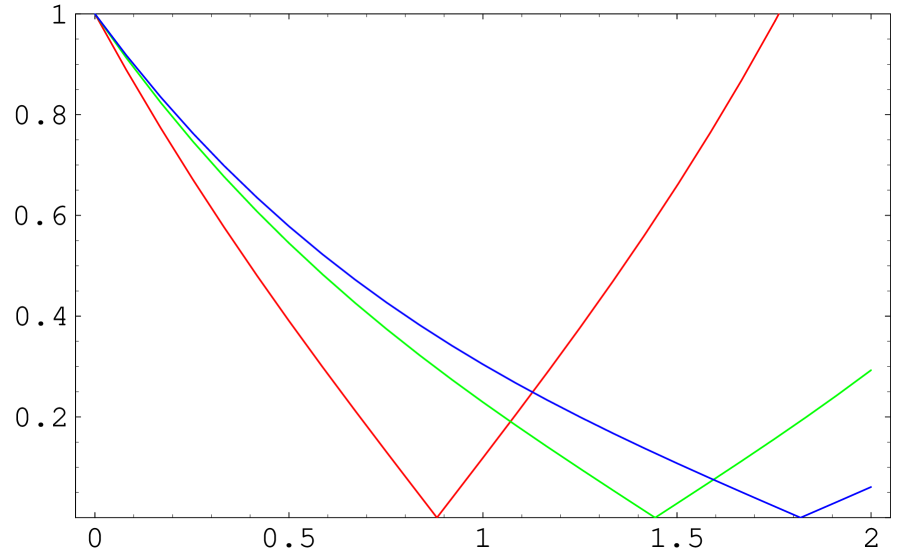
Figure 1: The function $f(z)$ has a zero at $z_{max}$. The red line is for the case with $\ell=1$, $\tilde{r}_{A}=0.5$, the green one for $\ell=1$, $\tilde{r}_{A}=2$, and the blue one for $\ell=1$, $\tilde{r}_{A}=3$, respectively.

Once the bulk geometry is known, we can calculate the area of the apparent horizon using the bulk geometry. Let us first consider the case with $n=4$. Considering the $\mathbb{Z}_{2}$ symmetry, we have the horizon area

$$\mathcal{A}=2\times 4\pi\tilde{r}_{A}^{2}\int_{0}^{z_{max}}f^{2}(z,\tilde{r}_{A})dz\,,$$ (78)

Carrying out the integration, we arrive at

$$\mathcal{A}=4\pi\tilde{r}_{A}^{2}\ell\left[\sqrt{1+\frac{\ell^{2}}{\tilde{r}_{A}^{2}}}-\frac{\ell^{2}}{\tilde{r}_{A}^{2}}\mathrm{arcsinh}\left(\frac{\tilde{r}_{A}}{\ell}\right)\right]\,.$$ (79)

According to the $5$-dimensional area formula, we obtain the entropy associated with this $5$-dimensional apparent horizon

$$S=\frac{A_{2}}{4G_{5}}\ell\left[\sqrt{1+\frac{\ell^{2}}{\tilde{r}_{A}^{2}}}-\frac{\ell^{2}}{\tilde{r}_{A}^{2}}\mathrm{arcsinh}\left(\frac{\tilde{r}_{A}}{\ell}\right)\right]\,.$$ (80)

Using the relation (22), we can rewrite this entropy as

$$S=\frac{A_{2}}{4G_{4}}\left[\sqrt{1+\frac{\ell^{2}}{\tilde{r}_{A}^{2}}}-\frac{\ell^{2}}{\tilde{r}_{A}^{2}}\mathrm{arcsinh}\left(\frac{\tilde{r}_{A}}{\ell}\right)\right]\,.$$ (81)

This is exactly the form (46) we have given in the previous section by using the method developed in [6].

For the case with an arbitrary $n$ ($n>4$), the area of the apparent horizon in the $(n+1)$-dimensional bulk can be expressed as

$$\mathcal{A}=2\times\Omega_{n-2}\tilde{r}_{A}^{n-2}\int_{0}^{z_{max}(\tilde{r}_{A})}f^{n-2}(z,\tilde{r}_{A})dz\,.$$ (82)

After some calculations, one can obtain

$$\mathcal{A}=\frac{2}{n-1}\Omega_{n-2}\tilde{r}_{A}^{n-1}{}_{2}F_{1}\left[\frac{n-1}{2},\frac{1}{2},\frac{n+1}{2},-\left(\frac{\tilde{r}_{A}}{\ell}\right)^{2}\right]\,.$$ (83)

By using the $(n+1)$-dimensional area formula of horizon entropy, we have

$$S=\frac{\mathcal{A}}{4G_{n+1}}=\frac{A_{n-2}}{4G_{n+1}}\frac{2\ell}{n-1}\left(\frac{\tilde{r}_{A}}{\ell}\right){}_{2}F_{1}\left[\frac{n-1}{2},\frac{1}{2},\frac{n+1}{2},-\left(\frac{\tilde{r}_{A}}{\ell}\right)^{2}\right]\,.$$ (84)

Using the relation (22), once again, we arrive at

$$S=\frac{A_{n-2}}{4G_{n}}\Bigg{\{}\frac{n-2}{n-1}\left(\frac{\tilde{r}_{A}}{\ell}\right){}_{2}F_{1}\left[\frac{n-1}{2},\frac{1}{2},\frac{n+1}{2},-\left(\frac{\tilde{r}_{A}}{\ell}\right)^{2}\right]\Bigg{\}}\,.$$ (85)

This is completely the same as the entropy expression (45) associated with the apparent horizon on the brane.

Clearly, when the bulk Weyl tensor is nonvanished, one has to solve a nonlinear second-order differential equation for $n>4$, in order to give the bulk geometry. Solving this nonlinear equation is not an easy matter, but it is worth trying. Once the bulk geometry is given, one can obtain the entropy of apparent horizon by using the area formula in the bulk.

5 Conclusion and discussion

In this paper we have discussed thermodynamics of the apparent horizon of an $n$-dimensional FRW universe in the RSII brane world scenario. The gravity theory on the brane is not the Einstein one due to the existence of extra dimension, therefore the well-known area formula for horizon entropy is not applicable on the brane. By using the method we have developed in [6], we have obtained an explicit entropy expression of the apparent horizon in the $n$-dimensional FRW universe embedded in an $(n+1)$-dimensional pure AdS space-time. In this model, the effective energy-momentum tensor coming from the non-Einstein part is just the $\pi_{\mu\nu}$ in the effective field equations on the brane. From this effective energy-momentum tensor, we define an effective energy-supply. By using the unified first law, together with the Clausius relation $\delta Q=\langle A\stackrel{{\scriptstyle m}}{{\Psi}},\xi\rangle=\frac{\kappa}{8\pi G}\langle dA,\xi\rangle-\langle A\stackrel{{\scriptstyle e}}{{\Psi}},\xi\rangle=TdS$ (This also suggests that the associated thermodynamics with the apparent horizon is an equilibrium one), we have obtained an analytic expression (45) of the entropy for the apparent horizon. The entropy expression has expected properties. In the limit of large horizon radius, this entropy reduces to the $n$-dimensional area formula, where the Einstein gravity on the brane is recovered. In this case, this entropy can be interpreted as the area of the “cylinder” as described in [24]. On the other hand, in the limit of small horizon radius, the entropy reduces to $(n+1)$-dimensional area formula, as respected, and can be interpreted as the area of two “disks”, which is negligible in the large radius limit. In addition, we have shown that the Friedmann equation on the brane can be rewritten as a universal form like the first law, $dE=TdS+WdV$.

Our entropy expression for the apparent horizon in FRW universe is useful in the study of thermodynamics of black holes on the brane since we expect that the entropy associated with apparent horizon and black hole horizon has a same expression.

We have also discussed the bulk geometry for an arbitrary dimension $n\geq 4$, and given a solution with vanishing Weyl tensor. We have found that the apparent horizon extends into the bulk with a finite distance which are labelled by $z_{max}(\tilde{r}_{A})=\ell\mathrm{arcsinh}\left(\tilde{r}_{A}/\ell\right)$. Using the bulk geometry and the area formula in the bulk, we have calculated the entropy associated with the apparent horizon extended into the bulk. We have found that both methods give the completely same expression for the apparent horizon entropy. It is of great interest to extend our method to other brane world scenarios such as DGP model, models with a bulk Gauss-Bonnet term, etc.

References

• [1] S. A. Hayward, Phys. Rev. D 49, 6467 (1994).
• [2] S. A. Hayward, Phys. Rev. D 53, 1938 (1996) [arXiv:gr-qc/9408002].
• [3] S. A. Hayward, Class. Quant. Grav.  15, 3147 (1998) [arXiv:gr-qc/9710089].
• [4] S. A. Hayward, S. Mukohyama and M. C. Ashworth, Phys. Lett. A 256, 347 (1999) [arXiv:gr-qc/9810006].
• [5] C. W. Misner and D. H. Sharp, Phys. Rev.  136, B571 (1964).
• [6] R. G. Cai and L. M. Cao, Phys. Rev.  D 75, 064008 (2007) [arXiv:gr-qc/0611071].
• [7] R. G. Cai and S. P. Kim, JHEP 0502, 050 (2005)[arXiv:hep-th/0501055].
• [8] M. Akbar and R. G. Cai, Phys. Lett. B635, 7 (2006) [arXiv:hep-th/0602156].
• [9] A. V. Frolov and L. Kofman, JCAP 0305, 009(2003) [hep-th/0212327].
• [10] U. K. Danielsson, Phys. Rev. D71, 023516(2005) [arXiv: hep-th/0411172].
• [11] R. Bousso, Phys. Rev. D71, 064024 (2005) [arXiv: hep-th/0412197].
• [12] G. Calcagni, JHEP 0509, 060 (2005) [arXiv:hep-th/0507125].
• [13] M. Akbar and R. G. Cai, Phys. Rev.  D 75, 084003 (2007) [arXiv:hep-th/0609128].
• [14] M. Akbar and R. G. Cai, Phys. Lett.  B 648, 243 (2007) [arXiv:gr-qc/0612089].
• [15] T. Padmanabhan, Class. Quant. Grav. 19, 5387 (2002)[arXiv: gr-qc/0204019]; Phys. Rept. 406, 49 (2005)[arXiv: gr-qc/0311036]; T. Padmanabhan, arXiv:gr-qc/0606061.
• [16] A. Paranjape, S. Sarkar, and T. Padmanabhan, Phys. Rev. D74, 104015 (2006) [arXiv: hep-th/0607240].
• [17] T. Jacobson, Phys. Rev. Lett. 75, 1260 (1995).
• [18] C. Eling, R. Guedens, and T. Jacobson, Phys.Rev.Lett.96, 121301 (2006) [arXiv:gr-qc/0602001].
• [19] P. Binetruy, C. Deffayet, U. Ellwanger, D. Langlois, [arXiv:hep-th/9910219]
• [20] N. Arkani-Hamed, S. Dimopoulos and G. R. Dvali, Phys. Lett. B 429, 263 (1998) [arXiv:hep-ph/9803315]; I. Antoniadis, N. Arkani-Hamed, S. Dimopoulos and G. R. Dvali, Phys. Lett. B 436, 257 (1998) [arXiv:hep-ph/9804398].
• [21] L. Randall and R. Sundrum, Phys. Rev. Lett.  83, 3370 (1999) [arXiv:hep-ph/9905221].
• [22] L. Randall and R. Sundrum, Phys. Rev. Lett.  83, 4690 (1999) [arXiv:hep-th/9906064].
• [23] T. Shiromizu, K. i. Maeda and M. Sasaki, Phys. Rev. D 62, 024012 (2000) [arXiv:gr-qc/9910076]; A. N. Aliev and A. E. Gumrukcuoglu, Class. Quant. Grav.  21, 5081 (2004) [arXiv:hep-th/0407095].
• [24] R. Emparan, G. T. Horowitz and R. C. Myers, JHEP 0001, 007 (2000) [arXiv:hep-th/9911043].
• [25] D. Bak and S. J. Rey, Class. Quant. Grav.  17, L83 (2000) [arXiv:hep-th/9902173].