hep–th/0612139

Stability of strings dual to flux tubes
between static quarks in ${\cal N}=4$ SYM

Spyros D. Avramis^1,2,x Konstadinos Sfetsos¹x andx Konstadinos Siampos¹

${}^{1}\!$ Department of Engineering Sciences, University of Patras,

26110 Patras, Greece

${}^{2}\!$ Department of Physics, National Technical University of Athens,

15773, Athens, Greece

avramis@mail.cern.ch,   sfetsos@upatras.gr,   ksiampos@upatras.gr

Abstract

Computing heavy quark-antiquark potentials within the AdS/CFT correspondence often leads to behaviors that differ from what one expects on general physical grounds and field-theory considerations. To isolate the configurations of physical interest, it is of utmost importance to examine the stability of the string solutions dual to the flux tubes between the quark and antiquark. Here, we formulate and prove several general statements concerning the perturbative stability of such string solutions, relevant for static quark-antiquark pairs in a general class of backgrounds, and we apply the results to ${\cal N}=4$ SYM at finite temperature and at generic points of the Coulomb branch. In all cases, the problematic regions are found to be unstable and hence physically irrelevant.

1 Introduction

In the framework of the AdS/CFT correspondence [2], the computation of the static Wilson-loop quark-antiquark potential in ${\cal N}=4$ super Yang–Mills at large ’t Hooft coupling is mapped to the classical problem of minimizing the action for a string connecting the quark and antiquark on the boundary of ${\rm AdS}_{5}$ and extending into the radial direction. This approach was first employed in [3] for the conformal case and further extended in [4, 5] to non-conformal cases. Moreover, motivated by the recent interest in applying AdS/CFT ideas and techniques to calculations relevant to moving mesons in thermal plasmas, the finite-temperature calculations of this type have been extended in various ways [6]–[10].

Although in the conformal case these calculations reproduce the expected Coulomb behavior of the potential, in the non-conformal extensions there are cases where the behavior of the potential is quite different from what one anticipates based on expectations from the field-theory side. For instance, for finite-temperature ${\cal N}=4$ SYM, one encounters multiple branches of the quark-antiquark potential as well as a behavior resembling a phase transition, while for the Coulomb branch of ${\cal N}=4$ SYM one encounters a linear confining behavior at certain regions of the moduli space. To check whether these types of behavior are actually predicted by the gauge/gravity correspondence, one must subject the corresponding string configurations to certain consistency checks, one of which is their stability under small fluctuations.

For the conformal case, the equations of motion for the fluctuations have been first obtained in [11, 12] and result in a positive spectrum as expected. For the finite-temperature case, where two branches of the solution occur, the question of stability was investigated recently in [13] for the case of a moving quark-antiquark pair. For this problem, the small-fluctuation analysis yielded a system of coupled differential equations, and numerical investigations suggested that the long string corresponding to the upper branch of the potential is unstable against small perturbations in the longitudinal directions.

Here we will conduct a stability analysis, restricting ourselves to static configurations and pursuing an analytic treatment all the way. We will investigate perturbations in all coordinates including the angular ones and we will consider ${\cal N}=4$ SYM both at finite temperature and at the Coulomb branch. In this setting, the equations for the longitudinal, transverse and angular perturbations decouple and the problem is amenable to analytic methods. In particular, the strategy that we will employ is to write the equations of motion satisfied by the fluctuations in both Sturm–Liouville and Schrödinger forms and to deduce the frequency spectrum of the fluctuations either from the Sturm–Liouville zero modes or from the Schrödinger potentials, using both exact and approximate methods.

This article is organized as follows. In section 2, we describe the calculation of Wilson loops in the AdS/CFT framework via classical string configurations in D3-brane backgrounds and we discuss the general features of the resulting quark-antiquark potentials. In section 3, we consider small fluctuations about the classical solutions, we turn the equations of motion of these fluctuations into one-dimensional Schrödinger problems, and we establish several general results for the exact and approximate calculation of the corresponding energy eigenvalues. In section 4, we specialize the general calculations of section 2 to the cases of non-extremal and multicenter D3-branes and we identify certain regions of the parameter space for which the potentials fail to capture the behavior expected on physical grounds. In section 5, we apply the general stability analysis to these configurations and we prove that all regions where problematic behavior arises are perturbatively unstable. In section 6, we summarize and conclude. Finally, in the appendix we discuss an interesting analogy of our problem with the standard classical-mechanical problem of determining the shapes of a soap film stretching between two rings and their stability.

2 The classical solutions

Our general setup refers to the AdS/CFT calculation of the static potential of a heavy quark-antiquark pair according to the well-known recipe of [3] for the conformal case and its extensions [4, 5] beyond conformality. On the gauge-theory side, this potential is extracted from the expectation value of a rectangular Wilson loop with one temporal and one spatial side. On the gravity side, the Wilson loop expectation value is calculated by extremizing the Nambu–Goto action for a fundamental U-shaped string propagating into the dual supergravity background, whose endpoints are constrained to lie on the two temporal sides of the Wilson loop. Below, we give a brief review of this procedure, following [5], and we outline the main qualitative features of the resulting potentials.

We consider a general metric of the form

$$ds^{2}=G_{tt}dt^{2}+G_{yy}dy^{2}+G_{uu}du^{2}+G_{xx}dx^{2}+G_{\theta\theta}d\theta^{2}+\ldots\ ,$$ (2.1)

noting that we will use Lorentzian signature throughout the paper. Here, $y$ denotes the (cyclic) coordinate along which the spatial side of the Wilson loop extends, $u$ denotes the radial direction playing the rôle of an energy scale in the dual gauge theory and extending from the UV at $u\to\infty$ down to the IR at some minimum value $u_{\rm min}$ determined by the geometry, $x$ stands for a generic cyclic coordinate, $\theta$ stands for a generic coordinate on which the metric components may depend in a particular way to be specified shortly and the omitted terms involve coordinates that fall into one of the two latter classes. Note that the metric (2.1) is diagonal and that we do not consider off-diagonal terms in the present paper. For the analysis that follows, it is convenient to introduce the functions

$$g(u,\theta)=-G_{tt}G_{uu}\ ,\qquad f_{y}(u,\theta)=-G_{tt}G_{yy}\ ,$$ (2.2)

while for the stability analysis, we also introduce

$$f_{x}(u,\theta)=-G_{tt}G_{xx}\ ,\qquad f_{\theta}(u,\theta)=-G_{tt}G_{\theta\theta}\ ,\qquad h(u,\theta)=G_{yy}G_{uu}\ .$$ (2.3)

It is useful to mention the behavior of the above functions in the conformal limit, where the metric reduces to that of ${\rm AdS}_{5}\times{\rm S}^{5}$. Using the leading order expressions

$$-G_{tt}\simeq G_{xx}\simeq G_{yy}\simeq{u^{2}\over R^{2}}\ ,\quad G_{uu}\simeq{R^{2}\over u^{2}}\ ,\quad G_{\theta\theta}\simeq R^{2}\ ,\qquad{\rm as}\quad u\to\infty\ ,$$ (2.4)

we see that

$$g\simeq h\simeq 1\ ,\quad f_{x}\simeq f_{y}\simeq u^{4}\ ,\quad f_{\theta}\simeq u^{2}\ ,\qquad{\rm as}\quad u\to\infty\ .$$ (2.5)

In the framework of the AdS/CFT correspondence, the interaction potential energy of the quark-antiquark pair is given by

$$e^{-{\rm i}ET}=\langle W(C)\rangle=e^{{\rm i}S[C]}\ ,$$ (2.6)

where

$$S[C]=-{1\over 2\pi}\int d\tau d\sigma\sqrt{-\det g_{\alpha\beta}}\ ,\qquad g_{\alpha\beta}=G_{\mu\nu}\partial_{\alpha}x^{\mu}\partial_{\beta}x^{\nu}\ ,$$ (2.7)

is the Nambu–Goto action for a string propagating in the dual supergravity background whose endpoints trace the contour $C$. To proceed, we fix reparametrization invariance by choosing

$$t=\tau\ ,\qquad u=\sigma\ ,$$ (2.8)

we assume translational invariance along $t$, and we consider the embedding

$$y=y(u)\ ,\qquad x=0\ ,\qquad\theta=\theta_{0}={\rm const.}\ ,\qquad\hbox{rest}={\rm const.}\ ,$$ (2.9)

supplemented by the boundary condition

$$u\left(\pm{L\over 2}\right)=\infty\ ,$$ (2.10)

appropriate for a quark placed at $y=-L/2$ and an antiquark placed at $y=L/2$. In the ansatz (2.9), the constant value $\theta_{0}$ of the non-cyclic coordinate $\theta$ must be consistent with the corresponding equation of motion. As we shall see later on, this requires that

$$\partial_{\theta}g(u,\theta)|_{\theta=\theta_{0}}=\partial_{\theta}f_{y}(u,\theta)|_{\theta=\theta_{0}}=0\ ,$$ (2.11)

which is definitely satisfied if the metric components obey identical to the above vanishing relations. We note that there are occasions where the latter stronger condition is not satisfied but (2.11) is [14]. For the ansatz given above, the Nambu–Goto action reads

$$S=-{T\over 2\pi}\int du\sqrt{g(u)+f_{y}(u)y^{\prime 2}}\ ,$$ (2.12)

where $T$ denotes the temporal extent of the Wilson loop, the prime denotes a derivative with respect to $u$ while $g(u)\equiv g(u,\theta_{0})$ and $f_{y}(u)\equiv f_{y}(u,\theta_{0})$ are the functions in (2.2) evaluated at the chosen constant value $\theta_{0}$ of $\theta$. To seek a classical solution $y_{\rm cl}(u)$, we proceed by reducing the problem to quadrature. Independence of the Lagrangian from $y$ implies that the associated momentum is conserved, leading to the equation

$${f_{y}y_{\rm cl}^{\prime}\over\sqrt{g+f_{y}y_{\rm cl}^{\prime 2}}}=\pm f_{y0}^{1/2}\qquad\Longrightarrow\qquad y_{\rm cl}^{\prime}=\pm{\sqrt{f_{y0}F}\over f_{y}}\ ,$$ (2.13)

where $u_{0}$ is the value of $u$ at the turning point, $f_{y0}\equiv f_{y}(u_{0})$, $y_{\rm cl}$ is the classical solution with the two signs corresponding to the two symmetric branches around the turning point, and $F$ stands for the shorthand

$$F={gf_{y}\over f_{y}-f_{y0}}\ .$$ (2.14)

Integrating (2.13), we express the separation length as

$$L=2f_{y0}^{1/2}\int_{u_{0}}^{\infty}du{\sqrt{F}\over f_{y}}\ .$$ (2.15)

Finally, inserting the solution for $y_{\rm cl}^{\prime}$ into (2.12) and subtracting the divergent self-energy contribution of disconnected worldsheets, we write the interaction energy as

$$E={1\over\pi}\int_{u_{0}}^{\infty}du\sqrt{F}-{1\over\pi}\int_{u_{\rm min}}^{\infty}du\sqrt{g}\ .$$ (2.16)

Ideally, one would like to evaluate the integrals (2.15) and (2.16) exactly, solve (2.15) for $u_{0}$ and insert into (2.16) to obtain an expression for the energy $E$ in terms of the separation length $L$. However, in practice this cannot be done exactly, except for the simplest possible cases, and Eqs. (2.15) and (2.16) are to be regarded as parametric equations for $L$ and $E$ with parameter $u_{0}$. The resulting quark-antiquark potential $E(L)$ is required to satisfy the concavity condition [15]

$${dE\over dL}>0\ ,\qquad{d^{2}E\over dL^{2}}\leqslant 0\ ,$$ (2.17)

which is valid for any gauge theory, irrespective of its gauge group and matter content, and signifies that the force is always attractive and its magnitude is a never increasing function of the separation distance. In our case it has been shown that [5]

$${dE\over dL}={1\over 2\pi}f_{y0}^{1/2}>0\ ,\qquad{d^{2}E\over dL^{2}}={1\over 4\pi}{f^{\prime}_{y0}\over f^{1/2}_{y0}}{1\over L^{\prime}(u_{0})}\ ,$$ (2.18)

and, since in all known examples we have $f^{\prime}_{y0}>0$, the concavity condition restricts the physical range of the integration constant $u_{0}$ to the values where the inequality

$$L^{\prime}(u_{0})<0\$$ (2.19)

is satisfied.

In the archetypal example of [3] for ${\cal N}=4$ SYM, dual to a stack of D3-branes, Eq. (2.15) can be inverted for $u_{0}$ yielding a single-valued, monotonously decreasing, function of $L$ whose substitution into (2.16) gives the expected Coulomb potential, albeit with a coefficient which is proportional to $\sqrt{g_{\rm YM}^{2}N}$ rather than $g_{\rm YM}^{2}N$, presumably as a result of strong-coupling physics. This Coulombic behavior persists in the UV limit for all cases involving supergravity solutions that become asymptotically ${\rm AdS}_{5}\times{\rm S}^{5}$ as $u\to\infty$. However, towards the IR, the behavior of the potential is quite different and depends on the details of the supergravity solution. In particular, for ${\cal N}=4$ SYM at finite temperature, dual to a stack of non-extremal D3-branes [4], as well as for the Coulomb branch of ${\cal N}=4$ SYM, dual to multicenter distributions of D3-branes [5], one encounters three types of behavior, described below.

• A solution for $u_{0}=u_{0}(L)$ exists only for $L$ below a maximal value $L_{\rm c}=L(u_{0\rm c})$ and is a double-valued function of $L$. This signifies the existence of two classical string configurations satisfying the same boundary conditions, called a “short” string for $u_{0}>u_{0\rm c}$ and a “long” string for $u_{0}<u_{0\rm c}$, and satisfying $L^{\prime}(u_{0})<0$ and $L^{\prime}(u_{0})>0$ respectively. Accordingly, $E(L)$ is a double-valued function with the lower and upper branches corresponding to the short and long strings respectively. Although the upper branch is energetically disfavored, the classical analysis does not clarify whether the long string is perturbatively unstable or just metastable and hence physically realizable. The latter possibility would have been physically disturbing since it is conflict with the concavity condition (2.17) due to the fact that $L^{\prime}(u_{0})>0$ for this branch. Such a behavior has been encountered for ${\cal N}=4$ SYM at finite temperature and at certain regions of the Coulomb branch.

• A solution for $u_{0}$ exists only for $L$ below a maximal value $L_{\rm c}$ and it is a single-valued function of $L$. $E(L)$ is a single-valued function describing a screened Coulombic potential. However, the screening length is heavily dependent on the orientation of the string with respect to the brane distribution.

• A solution for $u_{0}$ exists for all $L$ and $E(L)$ is a single-valued function of $L$ interpolating between a Coulombic and a linear confining potential. However, a confining behavior is unexpected for the dual gauge theories under consideration due to the underlying conformal structure in combination with maximal supersymmetry.

  The last two types of behavior have been encountered for some regions of the Coulomb branch of ${\cal N}=4$ SYM. Note that in these cases it is not the concavity condition (2.17) that has been violated. The discrepancies arise due to the facts that ${\cal N}=4$ SYM at zero temperature is not expected to be a confining theory and that the screening length should not be a concept that depends heavily on the particular trajectory we use to compute the heavy quark interaction potential.

In all three cases, the behavior of the interaction energy as a function of the separation is quite puzzling and calls for a careful interpretation. For the first case under consideration, it is obvious that a small-fluctuation analysis will settle the issue whether the long string solution is perturbatively unstable. One might then be tempted to repeat the analysis for the two other cases, where there is no a priori indication about the stability of the solutions on energetic grounds. As it will turn out, such an analysis will cast as unstable the parametric regions that give rise to a heavily orientation-dependent screening length (in the second case), and a linear behavior (in the third case). It is quite impressive, in our opinion, that the small-fluctuation analysis suffices to resolve the puzzles in all three cases.

3 Stability analysis

Having described the basic features of the classical string solutions of interest, we now turn to a stability analysis of these configurations, with the aim of isolating the regions that are of physical interest and for which the gauge/gravity correspondence can be trusted. In this section we give a general description of the small-fluctuation analysis for the configurations discussed above with metric of the form (2.1) and we establish a series of results which will ultimately allow us to identify the stable and unstable regions by a combination of exact and approximate analytic methods.

3.1 Small fluctuations

To investigate the stability of the string configurations of interest, we consider small fluctuations about the classical solutions discussed above. In particular, we will be interested in three types of fluctuations, namely (i) “transverse” fluctuations, referring to cyclic coordinates transverse to the quark-antiquark axis such as $x$, (ii) “longitudinal” fluctuations, referring to the cyclic coordinate $y$ along the quark-antiquark axis, and (iii) “angular” fluctuations, referring to the special non-cyclic coordinate $\theta$. To parametrize the fluctuations about the equilibrium configuration, we perturb the embedding according to

$$x=\delta x(t,u)\ ,\qquad y=y_{\rm cl}(u)+\delta y(t,u)\ ,\qquad\theta=\theta_{0}+\delta\theta(t,u)\ .$$ (3.1)

keeping the gauge choice (2.8) unperturbed by using worldsheet reparametrization invariance. We then calculate the Nambu–Goto action for this ansatz and we expand it in powers of the fluctuations. The resulting expansion is written as

$$S=S_{0}+S_{1}+S_{2}+\ldots\ ,$$ (3.2)

where the subscripts in the various terms correspond to the respective powers of the fluctuations. The zeroth-order term gives just the classical action. The first-order contribution is easily seen to be

$$S_{1}=-{1\over 2\pi}\int dtdu\left[\sqrt{f_{y0}}\ \delta y^{\prime}+\left({1\over 2F^{1/2}}\partial_{\theta}g+{f_{y0}F^{1/2}\over 2f_{y}^{2}}\partial_{\theta}f_{y}\right)\delta\theta\right]\ ,$$ (3.3)

where $\partial_{\theta}g$ and $\partial_{\theta}f_{y}$ stand for the $\theta$–derivatives of the full functions $g(u,\theta)$ and $f_{y}(u,\theta)$, evaluated at $\theta=\theta_{0}$. The first term is a surface contribution which may cancelled out by adding to the classical action the boundary term which will not affect the classical equations of motion. In the second term, the coefficient of $\delta\theta$ is just the equation of motion of $\theta$ and the requirement that it vanish leads indeed to the condition (2.11). Using this condition and performing straightforward manipulations, we write the second-order contribution as

$$\!\!\!\!\!\!\!\!\!\!\!\!S_{2} = -{1\over 2\pi}\int dtdu\biggl{[}{f_{x}\over 2F^{1/2}}\delta x^{\prime 2}-{hf_{x}F^{1/2}\over 2gf_{y}}\delta\dot{x}^{2}$$

$$\qquad\qquad\quad\;+{gf_{y}\over 2F^{3/2}}\delta y^{\prime 2}-{h\over 2F^{1/2}}\delta\dot{y}^{2}$$

$$\qquad\qquad\quad\;+{f_{\theta}\over 2F^{1/2}}\delta\theta^{\prime 2}-{hf_{\theta}F^{1/2}\over 2gf_{y}}\delta\dot{\theta}^{2}+\left({1\over 4F^{1/2}}\partial_{\theta}^{2}g+{f_{y0}F^{1/2}\over 4f_{y}^{2}}\partial_{\theta}^{2}f_{y}\right)\delta\theta^{2}\biggr{]}\ ,$$

where all functions and their $\theta$–derivatives are again evaluated at $\theta=\theta_{0}$. We observe that, by virtue of (2.11), the various types of fluctuations decouple, which greatly facilitates the analysis. Writing down the equations of motion for this action, using independence of the various functions from $t$, and introducing an $e^{-{\rm i}\omega t}$ time dependence by setting

$$\delta x^{\mu}(t,u)=\delta x^{\mu}(u)e^{-{\rm i}\omega t}\ ,$$ (3.5)

we obtain the following linearized equations for the three types of fluctuations

$$\left[{d\over du}\left({f_{x}\over F^{1/2}}{d\over du}\right)+\omega^{2}{hf_{x}F^{1/2}\over gf_{y}}\right]\delta x=0\ ,$$

$$\left[{d\over du}\left({gf_{y}\over F^{3/2}}{d\over du}\right)+\omega^{2}{h\over F^{1/2}}\right]\delta y=0\ ,$$ (3.6)

$$\left[{d\over du}\left({f_{\theta}\over F^{1/2}}{d\over du}\right)+\left(\omega^{2}{hf_{\theta}F^{1/2}\over gf_{y}}-{1\over 2F^{1/2}}\partial_{\theta}^{2}g-{f_{y0}F^{1/2}\over 2f_{y}^{2}}\partial_{\theta}^{2}f_{y}\right)\right]\delta\theta=0\ .$$

Therefore, the problem of determining the stability of the string configurations of interest has reduced to a standard eigenvalue problem for the differential operators referring to the three types of fluctuation. More precisely, we are dealing with differential equations of the general Sturm–Liouville type

$$\left\{-{d\over du}\left[p(u;u_{0}){d\over du}\right]-r(u;u_{0})\right\}\Phi(u)=\omega^{2}q(u;u_{0})\Phi(u)\ ,\quad u_{\rm min}\leqslant u_{0}\leqslant u<\infty\ ,$$ (3.7)

where the functions $p(u;u_{0})$, $q(u;u_{0})$ and $r(u;u_{0})$ are read off from (3.1) and depend parametrically on $u_{0}$ through the function $F$ in (2.14). Our problem then is to determine the range of values of $u_{0}$ for which $\omega^{2}$ is negative, signifying an instability of the classical solution.

Although in many cases the Sturm–Liouville description given above is sufficient for our purposes, in other cases it will be convenient to transform our problem into a Schrödinger one. To do so, we employ the changes of variables

$$x=\int_{u}^{\infty}du\sqrt{q\over p}\ =\int_{u}^{\infty}du\sqrt{h\over f_{y}-f_{y0}}\ ,\qquad\Phi=(pq)^{-1/4}\Psi\ ,$$ (3.8)

where we note that the expression for $x$ is valid for all three types of fluctuations. Then, Eq. (3.7) is transformed to a standard Schrödinger equation

$$\left[-{d^{2}\over dx^{2}}+V(x;u_{0})\right]\Psi(x)=\omega^{2}\Psi(x)\ ,$$ (3.9)

with the potential

$$V=-{r\over q}+{p^{1/4}\over q^{3/4}}{d\over du}\left[\left({p\over q}\right)^{1/2}{d\over du}(pq)^{1/4}\right]=-{r\over q}+(pq)^{-1/4}{d^{2}\over dx^{2}}(pq)^{1/4}\ ,$$ (3.10)

expressed as a function $V(u;u_{0})$ of $u$ in the first relation and as a function $V(x;u_{0})$ of $x$ in the second one. The Schrödinger problem is defined in the range $x\in[0,x_{0}]$ where $x_{0}$ is given by

$$x_{0}=\int_{u_{0}}^{\infty}du\sqrt{q\over p}\ =\int_{u_{0}}^{\infty}du\sqrt{h\over f_{y}-f_{y0}}\ ,$$ (3.11)

and is finite, as can be verified using the asymptotic expressions (2.5) and the fact that $p/q\sim u-u_{0}$ as $u\to u_{0}$. The precise behavior of $x_{0}$ for finite values of the parameter $u_{0}$ depends on the details of the underlying supergravity solution. However, using the asymptotic expressions (2.5) we deduce that

$$x(u_{0})\simeq{\Gamma(1/4)^{2}\over 4\sqrt{2\pi}\ u_{0}}\ ,\qquad{\rm as}\quad u_{0}\to\infty\ .$$ (3.12)

The fact that the size of the interval is finite implies that the fluctuation spectrum is quantized and the fact that it becomes narrower in the UV implies that there cannot be any instability in the conformal limit of the theory. With the transformation (3.8) the UV and IR regions are mapped to the regions near $x=0$ and near $x=x_{0}$ respectively. In the Schrödinger description, our problem is to determine the range of $u_{0}$ for which the ground state of the potential in (3.10) has negative energy. Note that, in general, the first of (3.8) does not lead to a closed expression for $u$ in terms of $x$ and therefore it is not always possible to write down the potential as an explicit function of $x$. Nevertheless, in many cases the expression for the potential as a function of $u$ provides useful information by itself (for example, if $V(u;u_{0})$ is manifestly positive then the energy eigenvalues $\omega^{2}$ are always positive and no instability occurs), while its transcription in terms of $x$ may be easily accomplished when performing perturbation-theory calculations.

3.2 Boundary conditions

To fully specify our eigenvalue problem, we must impose appropriate boundary conditions on the fluctuations at the UV limit $u\to\infty$ ($x=0$) and at the IR limit $u=u_{0}$ ($x=x_{0}$). Starting from the Sturm-Liouville description, the boundary condition at the UV is particularly easy to determine by looking at the singularity structure of the differential equations in (3.1) as $u\to\infty$. Indeed, at this limit we find

$$\Phi^{\prime\prime}+{4\over u}\Phi^{\prime}={\cal O}(u^{-4})\ ,\qquad{\rm as}\quad u\to\infty\ ,$$ (3.13)

which implies that $u=\infty$ is a regular singular point and that the two independent solutions of any equation in (3.1) have the form

$$\Phi_{1} = \sum_{n=0}c_{n}u^{-n}\ ,$$

$$\Phi_{2} = d\ln u+{1\over u^{3}}\sum_{n=0}^{\infty}d_{n}u^{-n}\ .$$ (3.14)

For the first solution, which is regular at infinity, we use the freedom to assign to the constant $c_{0}$ any value we want to set it to zero. For the second solution, which blows up at infinity, we choose $d=0$. Hence we impose the boundary condition

$$\Phi(u)=0\ ,\qquad{\rm as}\quad u\to\infty\ .$$ (3.15)

The nature of the boundary condition at the IR needs special attention due to the fact that we have to glue the fluctuations around the upper and lower branches of the classical solution $y_{\rm cl}$, corresponding to the two different signs in (2.13). The point $u=u_{0}$ is again a regular singular point and the two independent solutions admit expansions of the form

$$\Phi_{1} = (u-u_{0})^{\rho}\left[c_{0}+\sum_{n=1}^{\infty}c_{n}(u-u_{0})^{n}\right]\ ,$$

$$\Phi_{2} = d_{0}+\sum_{n=1}^{\infty}d_{n}(u-u_{0})^{n}\ ,$$ (3.16)

where $\rho=1/2$ for the fluctuations along $x$ and $\theta$ and $\rho=-1/2$ for those along $y$. We demand that, on the two sides of the classical solution, the fluctuations and their first derivatives with respect to the classical solution be equal. However, this should be done not using the classical solution $y_{\rm cl}$, but that combined with its perturbation as in (3.1). Equivalently, defining a new coordinate $\bar{u}$ as

$$u=\bar{u}+\delta u(t,u)\ ,\qquad\delta u(t,u)=-{\delta y(t,u)\over y^{\prime}_{\rm cl}(u)}\ ,$$ (3.17)

the classical solution is not perturbed at all. This redefinition does not affect the $x$– and $\theta$–fluctuations since they have trivial classical support and we keep only linear in fluctuations terms. However, since $y_{\rm cl}^{\prime}\sim(u-u_{0})^{-1/2}$ near $u=u_{0}$, the fluctuation $\delta u$ has an expansion as in (3.16), but with $\rho=1/2$. Since, around the matching point, the two branches of the classical solution differ by a sign while the fluctuations are equal, we have

$${d\Phi\over dy_{\rm cl}}\bigg{|}_{u=u_{0}}=0\ ,$$ (3.18)

where $\Phi$ refers to the $\delta x,\delta\theta$ and $\delta u$ fluctuations. Recasting everything in terms of the original fluctuations we see that, in the expansions (3.16), the coefficient $c_{0}=0$ for the $x$ and $\theta$ fluctuations and $d_{0}=0$ for the $y$ ones. Equivalently,

$$\delta x,\delta\theta: \phantom{xxx}(u-u_{0})^{1/2}\Phi^{\prime}=0\ ,\qquad{\rm as}\quad u\to u_{0}^{+},$$

$$\delta y: \phantom{xxx}\Phi+2(u-u_{0})\Phi^{\prime}=0\ ,\qquad{\rm as}\quad u\to u_{0}^{+}\ .$$ (3.19)

These boundary conditions for the Sturm–Liouville function $\Phi$ can be transcribed to boundary conditions for the Schrödinger wavefunction $\Psi$ by using the asymptotic relations $u\sim 1/x$ for $u\to\infty$ and $u-u_{0}\sim(x_{0}-x)^{2}$ for $u\to u_{0}$ and $x\to x_{0}$, which follow from (3.8) and the asymptotic behavior of the $p$– and $q$–functions. After some manipulations, we find that for all types of fluctuations we must have

$$\Psi(0)=0\ ,\qquad\Psi^{\prime}(x_{0})=0\ ,$$ (3.20)

which correspond to a Dirichlet and a Neumann boundary condition, in the UV and IR respectively.

3.3 Zero modes

The method described above would in principle allow us to determine the regions of stability of the solutions, provided that the relevant Sturm–Liouville or Schrödinger problems could be solved exactly. However, in many cases, these problems are quite complicated and the spectrum is impossible to determine. On the other hand, it turns out that we can obtain useful information by studying a simpler problem, namely the zero-mode problem of the associated differential operators. In what follows, we prove that (i) transverse zero modes do not exist, (ii) longitudinal zero modes are in one-to-one correspondence with the critical points of the function $L(u_{0})$, and (iii) the angular zero-mode spectrum can be obtained to good accuracy by approximating the corresponding Schrödinger potential by an infinite square well. These results are crucial for the stability analysis of section 5.

3.3.1 Transverse zero modes

We consider first the case of the transverse fluctuations. The zero mode solution obeying (3.15) is up to a multiplicative constant

$$\delta x = \int^{\infty}_{u}{du\over f_{x}}\sqrt{gf_{y}\over f_{y}-f_{y0}}$$

$$= -2{\sqrt{gf_{y}}\over f_{x}f_{y}^{\prime}}\sqrt{f_{y}-f_{y0}}-2\int_{u}^{\infty}du\sqrt{f_{y}-f_{y0}}\partial_{u}\left(\sqrt{gf_{y}}\over f_{x}f_{y}^{\prime}\right)$$

$$= -2\int_{u_{0}}^{\infty}du\sqrt{f_{y}-f_{y0}}\ \partial_{u}\left(\sqrt{gf_{y}}\over f_{x}f_{y}^{\prime}\right)-{2\over f_{x0}}\ \sqrt{g_{0}f_{y0}\over f^{\prime}_{y0}}(u-u_{0})^{1/2}+{\cal O}(u-u_{0})\ ,$$

where in the second step we performed a partial integration. The zero mode solution exists provided that we can satisfy the boundary condition (3.2), i.e. make the coefficient of $(u-u_{0})^{1/2}$ vanish for some value of the parameter $u_{0}$. It is easy to see that this is not possible and so transverse zero modes do not exist. Therefore, if the lowest eigenvalue of the Schrödinger operator corresponding to the transverse fluctuations is positive for some value of $u_{0}$, it will stay positive throughout. Since, as it will turn out, this is indeed the case for all situations under consideration, the classical solutions are stable under transverse perturbations.

3.3.2 Longitudinal zero modes

We next turn to the longitudinal fluctuations, for which we will prove the powerful result that normalizable zero modes exist only at the values of $u_{0}$ where the length function $L(u_{0})$ in (2.15) has a critical point, i.e. $L^{\prime}(u_{0})=0$. The importance of this result lies in the fact that it implies that a point where the lowest eigenvalue $\omega^{2}$ changes sign must necessarily be a critical point of the length function.

To establish the connection between longitudinal zero modes and critical points of the length function, we begin by writing the longitudinal zero-mode solution obeying (3.13). Up to a multiplicative constant, we have

$$\delta y = \int^{\infty}_{u}du{\sqrt{gf_{y}}\over(f_{y}-f_{y0})^{3/2}}$$

$$= 2{1\over f^{\prime}_{y}}\sqrt{gf_{y}\over f_{y}-f_{y0}}+2\int_{u}^{\infty}{du\over\sqrt{f_{y}-f_{y0}}}\partial_{u}\left(\sqrt{gf_{y}}\over f_{y}^{\prime}\right)$$

$$= 2\sqrt{g_{0}f_{y0}\over f_{y0}^{\prime 3}}\ (u-u_{0})^{-1/2}+2\int_{u_{0}}^{\infty}{du\over\sqrt{f_{y}-f_{y0}}}\ \partial_{u}\left(\sqrt{gf_{y}}\over f_{y}^{\prime}\right)+{\cal O}\left((u-u_{0})^{1/2}\right)\ .$$

Then, the boundary condition (3.2) implies that this mode exists only if

$$\int_{u_{0}}^{\infty}{du\over\sqrt{f_{y}-f_{y0}}}\ \partial_{u}\left(\sqrt{gf_{y}}\over f_{y}^{\prime}\right)=0\ .$$ (3.23)

We next differentiate the length function (2.15) with respect to $u_{0}$. The result is easily seen to be

$$L^{\prime}(u_{0}) = {f_{y0}^{\prime}\over\sqrt{f_{y0}}}\int_{u_{0}}^{\infty}du{\sqrt{gf_{y}}\over(f_{y}-f_{y0})^{3/2}}-2f_{y0}^{1/2}{F^{1/2}\over f_{y}}\biggr{|}_{u=u_{0}}$$

$$= 2{f_{y0}^{\prime}\over\sqrt{f_{y0}}}\int_{u_{0}}^{\infty}{du\over\sqrt{f_{y}-f_{y0}}}\ \partial_{u}\left(\sqrt{gf_{y}}\over f_{y}^{\prime}\right)$$

$$+{2\over f_{y0}^{1/2}}\lim_{u\to u_{0}}\left[F^{1/2}\left({\partial_{u_{0}}f_{y0}\over\partial_{u}f_{y}}-{f_{y0}\over f_{y}}\right)\right]\ ,$$

where as before we have performed a partial integration. The last line is zero, so that

$$L^{\prime}(u_{0})=2{f_{y0}^{\prime}\over\sqrt{f_{y0}}}\int_{u_{0}}^{\infty}{du\over\sqrt{f_{y}-f_{y0}}}\ \partial_{u}\left(\sqrt{gf_{y}}\over f_{y}^{\prime}\right)\ ,$$ (3.25)

which is manifestly finite, in contrast with the first line in (3.3.2) where both terms diverge. Comparing (3.23) and (3.25) we see that at the extrema of $L(u_{0})$ there is a zero mode, as advertised. As a result, given the critical points of the length function, we can determine the sign of the lowest eigenvalue $\omega^{2}$ in all regions by expanding the Schrödinger potential in $u_{0}$ about each critical point $u_{0\rm c}$ and determining whether $\omega^{2}$ changes sign there.

There is an alternative way to understand the occurrence of the critical value $u_{0\rm c}$ in the above analysis. It is not difficult to prove that the Schrödinger potential has the following behavior at the extreme values of $u$, namely that

$$V(u;u_{0})=2u^{2}\ ,\qquad{\rm as}\quad u\to\infty\ ,$$ (3.26)

and

$$V_{0}(u_{0})=V(u_{0};u_{0})={f_{y0}^{\prime\prime}\over 2h_{0}}+{h_{0}^{\prime}f_{y0}^{\prime}\over 8h_{0}^{2}}-{3\over 8}{f_{y0}^{\prime}\over h_{0}}\left({g_{0}^{\prime}\over g_{0}}+{f_{y0}^{\prime}\over f_{y0}}\right)\ .$$ (3.27)

Since the potential rises from a minimum value to infinity in the finite interval $x\in[0,x_{0}]$, where $x_{0}$ is given by (3.11), the spectrum of fluctuations is discrete. In addition, if its minimum value $V_{0}$ is negative enough the potential can very well support bound states with negative energy and this happens whenever (3.23) has a solution for some values of the parameter $u_{0}$. The largest of these values is $u_{0\rm c}$ in which the lowest energy eigenvalue becomes zero.

3.3.3 Angular zero modes

We finally consider the angular zero modes which, unlike the two other types of zero modes, cannot be explicitly written in an integral form due to the presence of the “restoring force” term in the corresponding Sturm–Liouville equation at the third line of (3.1). On the other hand, in the Schrödinger description, we can obtain the full fluctuation spectrum to quite high accuracy by approximating the corresponding potential by an infinite well. The procedure is described below.

We first note that the behavior of the angular Schrödinger potentials at the limits $u\to\infty$ and $u=u_{0}$ in all our examples is as follows

$$V_{\infty}(u_{0})\equiv V(\infty;u_{0})={1\over 2}\lim_{u\to\infty}u^{2}\partial_{\theta}^{2}g\ ,$$ (3.28)

and

$$V_{0}(u_{0})\equiv V(u_{0};u_{0})={1\over 8}{g_{0}f_{y0}f_{y0}^{\prime}\over h_{0}^{2}f_{\theta 0}^{2}}\ \partial_{u_{0}}\left(h_{0}f_{\theta 0}^{2}\over g_{0}f_{y0}\right)+{1\over 2}{g_{0}\over h_{0}f_{\theta 0}}\partial^{2}_{\theta}f_{y0}\ .$$ (3.29)

where the limit in the first equation is finite. Since the potential rises from a minimum value to infinity in the finite interval $x\in[0,x_{0}]$, where $x_{0}$ is given by (3.11), we may approximate it by an infinite well given by

$$V_{\rm approx}=\left\{\begin{array}[]{l l}{1\over 2}(V_{0}+V_{\infty}),\quad 0\leqslant x\leqslant x_{0}\\ \infty\ ,\quad{\rm otherwise}\end{array}\right\}\ .$$ (3.30)

With the boundary conditions (3.20) the energy spectrum is given by

$$\omega^{2}_{n}(u_{0})={\pi^{2}(2n+1)^{2}\over 4[x_{0}(u_{0})]^{2}}+{1\over 2}\left[V_{0}(u_{0})+V_{\infty}(u_{0})\right]\ ,\qquad n=0,1,\dots\ .$$ (3.31)

Note that we have taken the average value of the values of the potential at the two extreme values of $u$. In order for a solution to exist, the above average must be negative at least in a finite range of values for $u_{0}$. The critical value $u_{0\rm c}$ is then obtained by numerically solving the equation $\omega^{2}_{0}(u_{0})=0$. We note that different choices for $V_{\rm approx}$ are possible (e.g. the average value of the potential itself) but, conceptually, they do not offer something new.

The advantage of the method just described is that it gives approximately the entire spectrum of fluctuations and its dependence on the parameter $u_{0}$ without the need for more sophisticated numerics. In particular, we may plot the lowest eigenvalue $\omega^{2}_{0}$ as a function of $u_{0}$ and easily check whether it is monotonously increasing function, as it is in all of our examples. In addition we will see that, in one case, the infinite-well approximation is in fact exact. Finally, we will show that there is a hierarchy of different critical values $u_{0{\rm c},n}$, $n=0,1,\dots$, with $u_{0\rm c}\equiv u_{0{\rm c},0}$ and $u_{0{\rm c},n}>u_{0{\rm c},n+1}$, at which the corresponding eigenvalues $\omega^{2}_{n}$ become zero and below which they become negative.

At this point one might wonder whether this infinite-well approximation could be applied to the longitudinal fluctuations, using, for example, (3.27) for the value of the potential at the bottom of the well, to yield in addition the full approximate spectrum of fluctuations. For our specific examples, it can be shown that, although such a choice gives a reasonable approximation to the result for $u_{0\rm c}$ following from (3.23), it also results in a tower of negative eigenvalues as we lower $u_{0}$, which is in conflict with our general conclusions following from (3.27). The discrepancy is traced to the fact that the true potential varies significantly during the interval $[0,x_{0}]$ and thus supports fewer negative-energy states than the infinite-well potential used to approximate it. One may of course devise phenomenological potentials that mimic the expected behavior, but there is no need to do so in the present context.

3.4 Perturbation theory

As stated earlier on, the stability of the solutions against longitudinal perturbations will be determined by identifying the critical points of $L(u_{0})$ and solving the Schrödinger equation for small deviations of $u_{0}$ from each critical point $u_{0\rm c}$ by means of perturbation theory. In doing so, we must note that the parameter $u_{0}$ enters into the problem not only by appearing explicitly in the potential $V(x;u_{0})$, but also by controlling the size of the interval $x_{0}$ in which the problem is defined. In what follows, we will present the perturbation-theory formulas that are appropriate for such a case.

To this end, we consider a more general Schrödinger problem defined on the interval $[0,x_{0}]$ with a potential that depends on a parameter $u_{0}$, for which we know that for some $u_{0}=u_{0\rm c}$ and $x_{0}=x_{0\rm c}$ the Schrödinger equation (3.9) admits a single solution with a given eigenvalue $\omega^{2}$ (equal to zero in our cases of interest). We would like to determine the correction to the energy eigenvalue when $u_{0}$ and $x_{0}$ deviate from $u_{0\rm c}$ and $x_{0\rm c}$. An easy computation shows that the potential can be written as

$$V(x;u_{0}) = V(x;u_{0\rm c})+\delta V(x)\ ,$$

$$\delta V(x) = {\delta x_{0}\over x_{0\rm c}}\Big{[}2V(x;u_{0\rm c})+x\partial_{x}V(x;u_{0\rm c})\Big{]}+\delta u_{0}\partial_{u_{0\rm c}}V(x;u_{0\rm c})+\dots\ ,$$ (3.32)

where $x\in[0,x_{0\rm c}]$ while $\delta u_{0}=u_{0}-u_{0\rm c}$ and $\delta x_{0}=x_{0}-x_{0\rm c}$. Then, a careful computation, keeping track of boundary terms, gives the energy shift

$$\delta\omega^{2} = \int_{0}^{x_{0\rm c}}dx\ |\Psi(x)|^{2}\delta V(x)$$ (3.33)

$$= {\delta x_{0}\over x_{0\rm c}}\ \left\{2\omega^{2}+\left[{1\over 2}(\Psi^{*}\Psi^{\prime}+\Psi\Psi^{*\prime})-x\Big{[}|\Psi^{\prime}|^{2}+(\omega^{2}-V)|\Psi|^{2}\Big{]}\right]_{0}^{x_{0\rm c}}\right\}$$

$$+\ \delta u_{0}\ \int_{0}^{x_{0\rm c}}dx\ |\Psi(x)|^{2}\ \partial_{u_{0\rm c}}V(x;u_{0\rm c})\ ,$$

where the term $(\omega^{2}-V)|\Psi|^{2}$ can be alternatively written as $-{1\over 2}\left(\Psi^{\prime\prime}\Psi^{*}+\Psi^{*\prime\prime}\Psi\right)$ using the Schrödinger equation. In deriving this, we have to use the boundary conditions so that the unperturbed Hamiltonian is Hermitian, which is always the case when the boundary conditions are Dirichlet, Neumann or a linear combination thereof.

To apply this result to our case, we set $\omega^{2}=0$ and we note that the parameters $x_{0}$ and $u_{0}$ are related by (3.11). Then, the energy shift is found to be

$$\delta\omega^{2}=\delta u_{0}\left[x^{\prime}_{0}(u_{0\rm c})V(x_{0\rm c};u_{0\rm c})|\Psi(x_{0\rm c})|^{2}+\int_{0}^{x_{0\rm c}}dx\ |\Psi(x)|^{2}\ \partial_{u_{0\rm c}}V(x;u_{0\rm c})\right]\ ,$$ (3.34)

with $x_{0\rm c}=x_{0}(u_{0\rm c})$ and where we have used the boundary conditions (3.20). Regarding the first term, an explicit computation, using (3.11), gives

$$x^{\prime}_{0}(u_{0})=f^{\prime}_{y0}\int_{u_{0}}^{\infty}du\ {\partial_{u}\left(h^{1/2}{f^{\prime}_{y}}^{-1}\right)\over\sqrt{f_{y}-f_{y0}}}\ .$$ (3.35)

Turning to the second term we must note that the $u_{0}$–derivative acts on the potential $V(x;u_{0})$ whose explicit form is not known. To transcribe this expression into one involving the potential $V(u;u_{0})$, for which explicit expressions are available, we must also take into account that when varying $u_{0}$ while keeping $x$ constant, $u$ varies as well. That is to say, $\partial_{u_{0}}V(x;u_{0})$ is actually the “convective” derivative

$$\partial_{u_{0}}V(x;u_{0})=\partial_{u_{0}}V(u;u_{0})+{\partial u\over\partial{u_{0}}}\ \partial_{u}V(u;u_{0})\ ,$$ (3.36)

where the second term can be evaluated with the aid of the expression

$${\partial u\over\partial u_{0}}={f^{\prime}_{y0}\over f^{\prime}_{y}}+f^{\prime}_{y0}\sqrt{f_{y}-f_{y0}\over h}\int_{u}^{\infty}du\ {\partial_{u}\left(h^{1/2}{f^{\prime}_{y}}^{-1}\right)\over\sqrt{f_{y}-f_{y0}}}\ .$$ (3.37)

Note that, in the case where (3.34) gives $\delta\omega^{2}=0$, we have to go beyond first-order perturbation theory to determine whether the energy eigenvalue changes sign. Luckily, no such behavior occurs in our examples.

4 D3-brane backgrounds: The classical solutions

In this section, we review the behavior of the quark-antiquark potentials emerging in Wilson-loop calculations for non-extremal and multicenter D3-brane backgrounds. The purpose of this review is to identify the three types of problematic behavior referred to at the end of section 2, which motivated our stability analysis. Since we will work with the Nambu–Goto action, we need mention in the expressions below only the metric and not the self-dual five-form which is the only other non-trivial field present in our backgrounds.

4.1 Non-extremal D3-branes

We start by considering a background describing a stack of $N$ non-extremal D3-branes. The field-theory limit of the metric reads

$$ds^{2}={u^{2}\over R^{2}}\left[-\left(1-{\mu^{4}\over u^{4}}\right)dt^{2}+d\vec{x}_{3}^{2}\right]+R^{2}\left({u^{2}\over u^{4}-\mu^{4}}\ du^{2}+d\Omega_{5}^{2}\right)\ ,$$ (4.1)

where the horizon is located at $u=\mu$ and the Hawking temperature is $T={\mu\over\pi R^{2}}$. This metric is just the direct product of ${\rm AdS}_{5}$–Schwarzschild with ${\rm S}^{5}$ and it is dual to ${\cal N}=4$ SYM at finite temperature. For the calculations that follow, it is convenient to switch to dimensionless variables by rescaling all quantities using the parameter $\mu$. Setting $u\to\mu u$ and $u_{0}\to\mu u_{0}$ and introducing dimensionless length and energy parameters by

$$L\to{R^{2}\over\mu}L\ ,\qquad E\to{\mu\over\pi}E\ ,$$ (4.2)

we see that all dependence on $\mu$ and $R$ drops out so that we may set $\mu\to 1$ and $R\to 1$ in what follows. The functions in (2.2) and (2.3) depend only on $u$ (reflecting the fact that all values of $\theta$ are equivalent) and are given by

$$g(u)=1\ ,\qquad f_{y}(u)=u^{4}-1\ ,$$ (4.3)

and

$$f_{x}(u)=u^{4}-1\ ,\qquad f_{\theta}(u)={u^{4}-1\over u^{2}}\ ,\qquad h(u)={u^{4}\over u^{4}-1}\ ,$$ (4.4)

respectively. From this it also follows that the equations of motion (2.11) for $\theta$ are identically satisfied for all values of $\theta_{0}$.

Let us now evaluate the quark-antiquark potential according to the guidelines of section 2. The integrals for the length and energy are given by [4, 5]

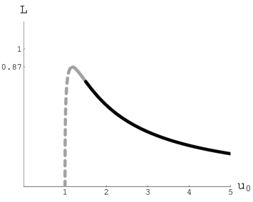
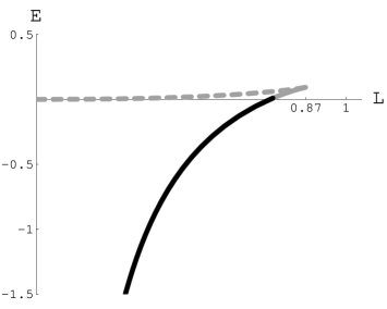
(a)	(b)

Figure 1: Plots of $L(u_{0})$ and $E(L)$ for the non-extremal D3-brane. In this and subsequent plots, the various types of lines correspond to stable (solid dark), metastable (solid gray) and unstable (dashed gray) configurations, with the stability determined by the analysis of section 5.

$$L=2\sqrt{u_{0}^{4}-1}\int_{u_{0}}^{\infty}{du\over\sqrt{(u^{4}-1)(u^{4}-u_{0}^{4})}}={2\sqrt{2}\pi^{3/2}\over\Gamma(1/4)^{2}}{\sqrt{u_{0}^{4}-1}\over u_{0}^{3}}{}_{2}F_{1}\left({1\over 2},{3\over 4},{5\over 4};{1\over u_{0}^{4}}\right)\ ,$$ (4.5)

and

$$E=\int_{u_{0}}^{\infty}du\left(\sqrt{{u^{4}-1\over u^{4}-u_{0}^{4}}}-1\right)-(u_{0}-1)=-{\sqrt{2}\pi^{3/2}\over\Gamma(1/4)^{2}}u_{0}\,{}_{2}F_{1}\left(-{1\over 2},-{1\over 4},{1\over 4};{1\over u_{0}^{4}}\right)+1\ ,$$ (4.6)

where ${}_{2}F_{1}(a,b,c;x)$ is the hypergeometric function and $u_{0}\geqslant 1$. For $u_{0}\gg 1$ the behavior is Coulombic while at the opposite limit, $u_{0}\to 1$, we have the asymptotics

$$L\simeq\sqrt{u_{0}-1}\left(\ln{8\over u_{0}-1}-{\pi\over 2}\right)\ ,\qquad E\simeq{u_{0}-1\over 2}\left(\ln{8\over u_{0}-1}-1-{\pi\over 2}\right)\ .$$ (4.7)

The function $L(u_{0})$ has a single global maximum, which together with the corresponding maximal length and energy are given by [5]

$$u_{\rm c}\simeq 1.177\ ,\qquad L_{\rm c}\simeq 0.869\ ,\qquad E_{c}\simeq 0.093\ .$$ (4.8)

For $L>L_{\rm c}$, only the disconnected solution exists. For $L<L_{\rm c}$, Eq. (4.5) has two solutions for $u_{0}$, corresponding to a short and a long string respectively and, accordingly, $E$ is a double-valued function of $L$. Moreover, there exists another value of the length, given in our case by $\tilde{L}_{\rm c}\simeq 0.754$, above which the disconnected configuration becomes energetically favored and the short string becomes metastable, which can be used as an alternative definition of the screening length. The behavior described above is shown in the plots of Fig. 1 and, provided that the upper branch of $E(L)$ is physically irrelevant, corresponds to a screened Coulomb potential.

4.2 Multicenter D3-branes

We now proceed to the case of multicenter D3-brane distributions. These were first constructed as the extremal limits of rotating D3-brane solutions [17, 18] in [19, 20] and belong to the rich class of continuous distributions of M- and string theory branes on higher dimensional ellipsoids [21]. These distributions have been used in several investigations within the AdS/CFT correspondence, starting with the works of [22, 5]. Here, we will concentrate on the particularly interesting cases of uniform distributions of D3-branes on a disc and on a three-sphere.

4.2.1 The disc

The field-theory limit of the metric for $N$ D3-branes uniformly distributed over a disc of radius $r_{0}$ reads

$$ds^{2} = H^{-1/2}(-dt^{2}+d\vec{x}_{3}^{2})+H^{1/2}{u^{2}+r_{0}^{2}\cos^{2}\theta\over u^{2}+r_{0}^{2}}\ du^{2}$$ (4.9)

$$+ H^{1/2}\left[(u^{2}+r_{0}^{2}\cos^{2}\theta)d\theta^{2}+r^{2}\cos^{2}\theta d\Omega_{3}^{2}+(u^{2}+r_{0}^{2})\sin^{2}\theta d\phi_{1}^{2}\right]\ ,$$

where

$$H={R^{4}\over u^{2}(u^{2}+r_{0}^{2}\cos^{2}\theta)}\ ,$$ (4.10)

while $d\Omega_{3}^{2}$ is the ${\rm S}^{3}$ metric. Since the only scale parameter entering into the supergravity solution is $r_{0}$ it is convenient to measure lengths and energies using this as a reference scale. Setting $u\to r_{0}u$ and $u_{0}\to r_{0}u_{0}$ and introducing the dimensionless length and energy parameters by

$$L\to{R^{2}\over r_{0}}L\ ,\qquad E\to{r_{0}\over\pi}E\ .$$ (4.11)

all dependence on $r_{0}$ and $R$ drops out so that we may set $r_{0}\to 1$ and $R\to 1$ in what follows. The functions in (2.2) and (2.3) now depend on $\theta$ and read

$$g(u,\theta)={u^{2}+\cos^{2}\theta\over u^{2}+1}\ ,\qquad f_{y}(u,\theta)=u^{2}(u^{2}+\cos^{2}\theta)\ ,$$ (4.12)

and

$$f_{x}(u,\theta)=u^{2}(u^{2}+\cos^{2}\theta)\ ,\qquad f_{\theta}(u,\theta)=u^{2}+\cos^{2}\theta\ ,\qquad h(u,\theta)={u^{2}+\cos^{2}\theta\over u^{2}+1}\ ,$$ (4.13)

respectively. The conditions (2.11) are satisfied only for $\theta_{0}=0$ and $\theta_{0}=\pi/2$, which correspond to trajectories orthogonal to the disc and lying on the plane of the disc, respectively. To evaluate the quark-antiquark potential, we examine these two trajectories in turn.

$\bullet$ $\theta_{0}=0$. For this case, the integrals for the dimensionless length and energy read [5]

$$L = 2u_{0}\sqrt{u_{0}^{2}+1}\int_{u_{0}}^{\infty}{du\over u\sqrt{(u^{2}+1)(u^{2}-u_{0}^{2})(u^{2}+u_{0}^{2}+1)}}$$ (4.14)

$$= {2u_{0}k^{\prime}\over u_{0}^{2}+1}\left[{\bf\Pi}(k^{\prime 2},k)-{\bf K}(k)\right]$$

and

$$E = \int_{u_{0}}^{\infty}du\left[u\sqrt{u^{2}+1\over(u^{2}-u_{0}^{2})(u^{2}+u_{0}^{2}+1)}-1\right]-u_{0}$$ (4.15)

$$= \sqrt{2u_{0}^{2}+1}\left[k^{\prime 2}{\bf K}(k)-{\bf E}(k)\right]\ ,$$

where ${\bf K}(k)$, ${\bf E}(k)$ and ${\bf\Pi}(\alpha,k)$ denote the complete elliptic integrals of the first, second and third kind respectively and

$$k={u_{0}\over\sqrt{2u_{0}^{2}+1}}\ ,\qquad k^{\prime}=\sqrt{1-k^{2}}\ ,$$ (4.16)

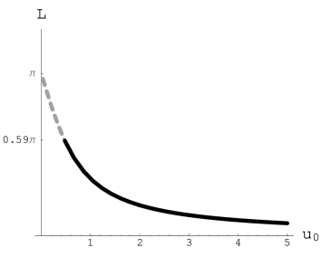
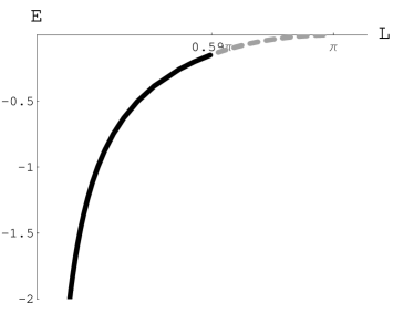
(a)	(b)

Figure 2: Plots of $L(u_{0})$ and $E(L)$ for the disc at $\theta_{0}=0$.

are the modulus and the complementary modulus. For $u_{0}\gg 1$, the behavior is Coulombic as before and at the opposite limit, $u_{0}\to 0$, we have the asymptotics [5]

$$L\simeq\pi(1-u_{0})\ ,\qquad E\simeq-{\pi\over 4}u_{0}^{2}\ ,$$ (4.17)

Now, $L(u_{0})$ is a monotonously decreasing function and hence its global maximum is at $u_{0{\rm c}}=0$ given by $L_{\rm c}=\pi$. For $L>L_{\rm c}$, only the disconnected solution exists, while for $L<L_{\rm c}$, Eq. (4.14) has a single solution for $u_{0}$ and $E$ is a single-valued function of $L$. This behavior is shown in the plots of Fig. 2, and it corresponds to a screened Coulomb potential.

$\bullet$ $\theta_{0}=\pi/2$. Now, the integrals for the dimensionless length and energy read

$$L = 2u_{0}^{2}\int_{u_{0}}^{\infty}{du\over u\sqrt{(u^{2}+1)(u^{4}-u_{0}^{4})}}$$ (4.18)

$$= {2u_{<}^{2}\over\sqrt{u_{0}^{2}+u_{>}^{2}}}\left[{\bf\Pi}\left({u_{>}^{2}\over u_{0}^{2}+u_{>}^{2}},k\right)-{\bf K}(k)\right]$$

and

$$E = \int_{u_{0}}^{\infty}duu\left[{u^{2}\over\sqrt{(u^{2}+1)(u^{4}-u_{0}^{4})}}-{1\over\sqrt{u^{2}+1}}\right]-\int_{0}^{u_{0}}{duu\over\sqrt{u^{2}+1}}$$ (4.19)

$$= {u_{0}^{2}\over\sqrt{u_{0}^{2}+u_{>}^{2}}}\ {\bf K}(k)-\sqrt{u_{0}^{2}+u_{>}^{2}}\ {\bf E}(k)+1\ ,$$

where now

$$k^{2}={u_{>}^{2}-u_{<}^{2}\over u_{0}^{2}+u_{>}^{2}}\ ,\qquad k^{\prime}=\sqrt{1-k^{2}}\$$ (4.20)

(a)	(b)

Figure 3: Plots of $L(u_{0})$ and $E(L)$ for the disc at $\theta_{0}=\pi/2$. Note that the screening length is less than the the one for $\theta_{0}=0$ by a factor of 2.

and $u_{>}$ ($u_{<}$) denotes the larger (smaller) between $u_{0}$ and $1$. At the limit $u_{0}\to 0$, we have the asymptotics [5]

$$L\simeq{\pi\over 2}\left[1-u_{0}^{2}\left(\ln{8\over u_{0}^{2}}-1\right)\right]\ ,\qquad E\simeq-{1\over 8}u_{0}^{4}\left(\ln{8\over u_{0}^{2}}-{3\over 2}\right)\ .$$ (4.21)

The behavior is qualitatively similar to the previous case with the maximal length being

$$L_{\rm c}={\pi\over 2}\ .$$ (4.22)

Comparing the $\theta_{0}=0$ and $\theta_{0}=\pi/2$ cases we note that, although the qualitative behavior of the potential is the same, the expressions for the screening length differ by a factor of 2. This factor is quite large as one expects that the orientation of the string configuration will have a mild effect on physical observables of the gauge theory. The apparent discrepancy will be resolved by our stability analysis.

4.2.2 The sphere

The field-theory limit of the metric for $N$ D3-branes uniformly distributed over a 3-sphere of radius $r_{0}$ reads

$$ds^{2} = H^{-1/2}(-dt^{2}+d\vec{x}_{3}^{2})+H^{1/2}{u^{2}-r_{0}^{2}\cos^{2}\theta\over u^{2}-r_{0}^{2}}\ du^{2}$$ (4.23)

$$+ H^{1/2}\left[(u^{2}-r_{0}^{2}\cos^{2}\theta)d\theta^{2}+u^{2}\cos^{2}\theta d\Omega_{3}^{2}+(u^{2}-r_{0}^{2})\sin^{2}\theta d\phi_{1}^{2}\right]\ ,$$

where

$$H={R^{4}\over u^{2}(u^{2}-r_{0}^{2}\cos^{2}\theta)}\ .$$ (4.24)

Note that this solution is obtained from the disc by taking $r_{0}^{2}\to-r_{0}^{2}$. Employing the same rescalings as before, we write the functions in (2.2) and (2.3) as

$$g(u,\theta)={u^{2}-\cos^{2}\theta\over u^{2}-1}\ ,\qquad f_{y}(u,\theta)=u^{2}(u^{2}-\cos^{2}\theta)\$$ (4.25)

and

$$f_{x}(u,\theta)=u^{2}(u^{2}-\cos^{2}\theta)\ ,\qquad f_{\theta}(u,\theta)=u^{2}-\cos^{2}\theta\ ,\qquad h(u,\theta)={u^{2}-\cos^{2}\theta\over u^{2}-1}\ ,$$ (4.26)

respectively, and the conditions (2.11) are again satisfied only for $\theta_{0}=0$ and $\theta_{0}=\pi/2$. We examine these two cases in turn.

$\bullet$ $\theta_{0}=0$. For this case, the integrals for the dimensionless length and energy read [5]

$$L = 2u_{0}\sqrt{u_{0}^{2}-1}\int_{u_{0}}^{\infty}{du\over u\sqrt{(u^{2}-1)(u^{2}-u_{0}^{2})(u^{2}+u_{0}^{2}-1)}}$$ (4.27)

$$= {2u_{0}k^{\prime}\over u_{0}^{2}-1}\left[{\bf\Pi}(k^{\prime 2},k)-{\bf K}(k)\right]$$

and

$$E = \int_{u_{0}}^{\infty}du\left[u\sqrt{u^{2}-1\over(u^{2}-u_{0}^{2})(u^{2}+u_{0}^{2}-1)}-1\right]-(u_{0}-1)$$ (4.28)

$$= \sqrt{2u_{0}^{2}-1}\left[k^{\prime 2}{\bf K}(k)-{\bf E}(k)\right]+1\ ,$$

where

$$k={u_{0}\over\sqrt{2u_{0}^{2}-1}}\ ,\qquad k^{\prime}=\sqrt{1-k^{2}}\ .$$ (4.29)

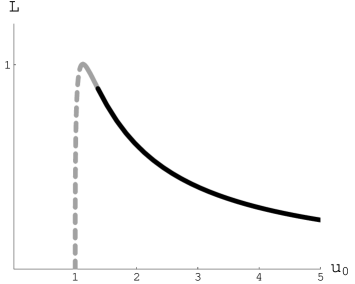
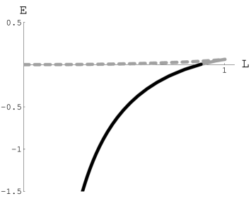
(a)	(b)

Figure 4: Plots of $L(u_{0})$ and $E(L)$ for the sphere at $\theta_{0}=0$. Note the appearance of two branches in the plot of $E(L)$.

For $u_{0}\gg 1$, the behavior is Coulombic, whereas in the opposite limit, $u_{0}\to 1$, we have the asymptotics [5]

$$L\simeq\sqrt{2(u_{0}-1)}\left[\ln\left({8\over u_{0}-1}\right)-2\right]\ ,\qquad E\simeq{u_{0}-1\over 2}\left[\ln\left({8\over u_{0}-1}\right)-3\right]\ .$$ (4.30)

The function $L(u_{0})$ has a single global maximum. Its location, its value and the corresponding value of the energy are [5]

$$u_{0\rm c}\simeq 1.125\ ,\qquad L_{\rm c}\simeq 1.002\ ,\qquad E_{c}\simeq 0.063\ .$$ (4.31)

For $L>L_{\rm c}$, only the disconnected solution exists. For $L<L_{\rm c}$, Eq. (4.27) has two solutions for $u_{0}$ and $E$ is a double-valued function of $L$. This behavior is shown in the plots of Fig. 4 and, discarding the upper branch of $E(L)$, it corresponds to a screened Coulomb potential.

$\bullet$ $\theta_{0}=\pi/2$. Now, the integrals for the dimensionless length and energy read

$$L=2u_{0}^{2}\int_{u_{0}}^{\infty}{du\over u\sqrt{(u^{2}-1)(u^{4}-u_{0}^{4})}}={\sqrt{2}\over u_{0}}\left[{\bf\Pi}\left({1\over 2},k\right)-{\bf K}(k)\right]\ ,$$ (4.32)

and

$$E=\int_{u_{0}}^{\infty}{duu\over\sqrt{u^{2}-1}}\left({u^{2}\over\sqrt{u^{4}-u_{0}^{4}}}-1\right)-\int_{1}^{u_{0}}{duu\over\sqrt{u^{2}-1}}={u_{0}\over\sqrt{2}}\left[{\bf K}(k)-2{\bf E}(k)\right]\ .$$ (4.33)

where now

$$k=\sqrt{{u_{0}^{2}+1\over 2u_{0}^{2}}}\ ,\qquad k^{\prime}=\sqrt{1-k^{2}}\ .$$ (4.34)

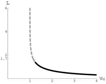
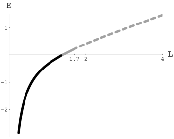
(a)	(b)

Figure 5: Plots of $L(u_{0})$ and $E(L)$ for the sphere at $\theta_{0}=\pi/2$. Note the appearance of a confining potential for large values of $L$.

For $u_{0}\gg 1$, the behavior is Coulombic, whereas in the opposite limit, $u_{0}\to 1$, we have the asymptotics [5]

$$L\simeq{1\over\sqrt{2}}\left[\ln\left({16\over u_{0}-1}\right)-2\sqrt{2}\ln(1+\sqrt{2})\right]\ ,\qquad E\simeq{1\over 2\sqrt{2}}\left[\ln\left({16\over u_{0}-1}\right)-4\right]\ .$$ (4.35)

Now, $L(u_{0})$ is a monotonously decreasing function which approaches infinity as $u_{0}\to 1$ and zero as $u_{0}\to\infty$ and hence no maximal length exists, Eq. (4.32) has a single solution for $u_{0}$, and $E$ is a single-valued function of $L$. Therefore, it seems that no screening occurs but, instead, from Eq. (4.35) we have a confining potential

$$E\simeq{L\over 2}\ ,\qquad{\rm for}\quad L\gg 1\ ,$$ (4.36)

whose appearance is quite puzzling, given that the underlying theory is ${\cal N}=4$ SYM.

Comparing the $\theta_{0}=0$ and $\theta_{0}=\pi/2$ cases, we note that the qualitative behavior of the potential appears to be completely different: in the first case the potential is a double-valued function of $L$ which exists up to a maximal length, whereas in the second case the potential exists for all values of the length and interpolates between a Coulombic and a confining potential. One does not expect such major qualitative differences to occur by a simple change of the orientation of the string and, moreover, the appearance of a confining potential is unexpected. Both of these issues will be resolved by our stability analysis.

5 D3-brane backgrounds: Stability analysis

In this section we apply the stability analysis developed in section 3 to the string solutions reviewed in section 4. We find that for the non-extremal D3-brane and the sphere with $\theta_{0}=0$ we have a longitudinal instability corresponding to the upper branch of the energy curve, while for the disc with $\theta_{0}=0$ and for the sphere with $\theta_{0}=\pi/2$ we have angular instabilities towards the IR, even though the potential has a single branch.

5.1 The conformal case

As a simple example, and as a consistency check, let us first consider the conformal case, corresponding to the $\mu\to 0$ or $r_{0}\to 0$ limit of any of the above solutions. In this case, the Schrödinger potentials read

$$V_{x}(u;u_{0}) = 2u^{2}\ ,$$

$$V_{\theta}(u;u_{0}) = 0\ ,$$ (5.1)

$$V_{y}(u;u_{0}) = 2{u^{4}-u_{0}^{4}\over u^{2}}\ ,$$

where the subscript indicates the corresponding fluctuating variable. The change of variables (3.8) explicitly gives

$$x={1\over u}\ {}_{2}F_{1}\left({1\over 2},{1\over 4},{5\over 4};{u_{0}^{4}\over u^{4}}\right)\ ,$$ (5.2)

and, hence, $x\in[0,x_{0}]$ with

$$x_{0}={\Gamma(1/4)^{2}\over 4\sqrt{2\pi}}\ {1\over u_{0}}\ .$$ (5.3)

Since all Schrödinger equations are defined in a finite interval with positive-definite potentials, the corresponding energy eigenvalues are positive and so there is no instability. The equations corresponding to (3.7) for the transverse ($\delta x$) and longitudinal ($\delta y$) fluctuations are given by Eq. (7) of [11] and Eq. (16) of [12] respectively. The comparison for $\delta x$ is immediate if we change variables as $u=1/z$ and also rename $z_{\rm m}=1/u_{0}$, where $z$ and $z_{\rm m}$ are the variable and parameter used in [11]. For $\delta y$, the comparison involves the same change of variables as before and $\delta y=u_{0}^{2}u^{2}(u^{4}-u_{0}^{4})^{-1/2}\delta\bar{y}$, where $\delta\bar{y}$ is the variable called $u$ in [12]. In addition, since the independent variable in Eq. (16) of [12] is $y$ ($x$ in their notation) we should also use the differential relation $dy=u_{0}^{2}/u^{2}(u^{4}-u_{0}^{4})^{-1/2}du$, resulting from the classical equation of motion (2.13).

5.2 Non-extremal D3-branes

We next proceed to the case of non-extremal D3-branes, where we recall that the potential energy is a double-valued function of the separation length. The Schrödinger potentials for the three types of fluctuations are given by

$$V_{x}(u;u_{0}) = 2{u^{8}-u_{0}^{4}\over u^{6}}\ ,$$

$$V_{\theta}(u;u_{0}) = 0\ ,$$ (5.4)

$$V_{y}(u;u_{0}) = 2{u^{12}-u_{0}^{4}u^{8}-(4u_{0}^{4}-3)u^{4}+u_{0}^{4}\over u^{6}(u^{4}-1)}\ .$$

The value of the endpoint $x_{0}$ is found using (3.11) and reads

$$x_{0}={\Gamma(1/4)^{2}\over 4\sqrt{2\pi}}\ {1\over u_{0}}\ {}_{2}F_{1}\left({1\over 2},{1\over 4},{3\over 4};{1\over u_{0}^{4}}\right)\ ,$$ (5.5)

with the behaviors (3.12) and

$$x_{0}(u_{0})\simeq-{1\over 4}\ln(u_{0}-1)+{\pi+\ln 64\over 8}+{\cal O}(u_{0}-1)\ .$$ (5.6)

Since $V_{x}$ is positive for all values of $u_{0}$, the solution is stable under transverse perturbations, in accordance with our general result in section 3.3. Also, $V_{\theta}$ is identically zero, which means that, given that $x_{0}$ is finite, the spectrum is positive-definite and the solution is stable against angular perturbations as well. On the other hand, $V_{y}$ starts from a negative value at $u=u_{0}$ given by

$$V_{y0}=-{8\over u_{0}^{2}}\ ,\qquad-8\leqslant V_{y0}<0\$$ (5.7)

and behaves as in (3.26) at $u\to\infty$. To examine the occurrence of instabilities under longitudinal perturbations, we apply the results of section 3.3 and the perturbation-theory formulas of section 3.4 to our problem. We find that there is a longitudinal zero mode at $u_{0}=u_{0\rm c}$ where $u_{0\rm c}$ is found by numerically solving the equation (3.23) which, for our case, reads

$${9\over 5u_{0}^{4}}\ {}_{2}F_{1}\left({1\over 2},{7\over 4},{9\over 4};{1\over u_{0}^{4}}\right)={}_{2}F_{1}\left({1\over 2},{3\over 4},{5\over 4};{1\over u_{0}^{4}}\right)\ .$$ (5.8)

This has precisely one solution given by the first of (4.8), i.e. $u_{0\rm c}\simeq 1.177$. To find the change in the energy eigenvalue $\omega^{2}$ as we move away from $u_{0\rm c}$, we first use (3.3.2) to find the explicit expression for the longitudinal zero mode

$$\delta y={1.463\over u^{3}}\ F{}_{1}\left({3\over 4};{3\over 2},-{1\over 2},{7\over 4};{u_{0\rm c}^{4}\over u^{4}},{1\over u_{0\rm c}^{4}}\right)\ ,$$ (5.9)

where $F{}_{1}(a\ ;b_{1},b_{2},c\ ;x,y)$ is the Appell hypergeometric function and the normalization has been fixed from the corresponding Schrödinger wavefunction which reads

$$\Psi={1.463\over u^{2}}\sqrt{u^{4}-u_{0\rm c}^{4}\over u^{4}-1}\ F{}_{1}\left({3\over 4};{3\over 2},-{1\over 2},{7\over 4};{u_{0\rm c}^{4}\over u^{4}},{1\over u_{0\rm c}^{4}}\right)\ .$$ (5.10)

Then, using Eq. (3.34), we find that the change in energy eigenvalue is given by

$$\delta\omega^{2}\simeq(51.9+29.6-20.1)\ \delta u_{0}=61.4\ \delta u_{0}\ ,$$ (5.11)

where each term inside the parentheses represents the contribution of the corresponding term in (3.34). Hence, as we move to the right (left) of $u_{0{\rm c}}$, the eigenvalue $\omega^{2}$ becomes positive (negative) and therefore the long string is unstable under longitudinal perturbations. This is what is expected from the energetics of these configurations, shown in Fig. 1(b).

5.3 Multicenter D3-branes

We finally turn to the case of multicenter D3-branes, where all types of problematic behavior discussed in section 2 appear. In what follows, we present the results of the stability analysis for all cases discussed in section 4.2.

5.3.1 The disc

For the disc distribution, we recall that both allowed orientations of the string lead to a screened Coulomb potential, but the screening lengths differ by a factor of 2. The results of the stability analysis for the two orientations are as follows.

$\bullet$ $\theta_{0}=0$. In this case, we have the Schrödinger potentials

$$V_{x}(u;u_{0}) = {8u^{8}+18u^{6}+11u^{4}-[2u_{0}^{2}(u_{0}^{2}+1)-1]u^{2}+u_{0}^{2}(u_{0}^{2}+1)\over 4u^{2}(u^{2}+1)^{2}}\ ,$$

$$V_{\theta}(u;u_{0}) = -{2u^{6}+u^{4}+[6u_{0}^{2}(u_{0}^{2}+1)-1]u^{2}+3u_{0}^{2}(u_{0}^{2}+1)\over 4u^{2}(u^{2}+1)^{2}}\ ,$$ (5.12)

$$V_{y}(u;u_{0}) = {8u^{8}+18u^{6}-[8u_{0}^{2}(u_{0}^{2}+1)-11]u^{4}-[6u_{0}^{2}(u_{0}^{2}+1)-1]u^{2}-3u_{0}^{2}(u_{0}^{2}+1)\over 4u^{2}(u^{2}+1)^{2}}\ ,$$

and the value of the endpoint $x_{0}$ reads

$$x_{0}=\sqrt{2{k^{\prime}}^{2}-1}\ {\bf K}(k^{\prime})\ ,$$ (5.13)

where $k^{\prime}$ is the complementary modulus defined in (4.16). We have the general behavior (3.12) and

$$x_{0}(u_{0})\simeq-\ln{u_{0}\over 4}+{\cal O}(u_{0}^{2}\ln u_{0})\ .$$ (5.14)

Since $V_{x}$ and $V_{y}$ are positive for all values of $u_{0}$, the solution is stable against transverse and longitudinal perturbations, in accordance with the general results of section 3.3 in the absence of a maximal length. On the other hand, $V_{\theta}$ is negative throughout the whole range of $u_{0}$, with its values at $u=u_{0}$ and $u\to\infty$ given by

$$V_{\theta 0} = -2+{3\over 2(u_{0}^{2}+1)}\ ,\qquad-2<V_{\theta 0}\leqslant-{1\over 2}\ ,$$

$$V_{\theta\infty} = -{1\over 2}\ .$$ (5.15)

To examine the occurrence of instabilities, we use the infinite-well approximation of (3.30) and we examine the behavior of the lowest eigenvalue $\omega_{0}^{2}$ by plotting it as a function of $u_{0}$. We find that it is an increasing function starting at negative values for $u_{0}=0$ and changing sign at a critical value $u_{0\rm c}$. This value, and the corresponding maximal length and energy, are given by

$$u_{0\rm c}\simeq 0.48\ ,\qquad L_{\rm c}\simeq 0.59\pi\ ,\qquad E_{\rm c}\simeq-0.15\ .$$ (5.16)

Therefore, when the separation distance of the quark-antiquark pair becomes larger than the value $L_{\rm c}$ given above, small fluctuations in $\theta$ destabilize the corresponding classical solution and the resulting potential should not be trusted. The true screening length is thus given by the second of (5.16) and turns out to be comparable to that for $\theta_{0}=\pi/2$. Moreover, within the infinite-well approximation, we may show that for $u_{0}<u_{0\rm c}$ more states become negative. Indeed, setting $\omega^{2}_{n}(u_{0})=0$ and using the limiting behavior (5.14), we find that the value $u_{0{\rm c},n}$ in which the $n$–th energy eigenvalue becomes zero is given by the formula

$$u_{0{\rm c},n}\simeq 4e^{-\pi(2n+1)/\sqrt{2}}\ ,$$ (5.17)

valid in practice for all $n\geqslant 1$.

$\bullet$ $\theta_{0}=\pi/2$. Now, the Schrödinger potentials are given by

$$V_{x}(u;u_{0}) = {2u^{6}+u^{4}+u_{0}^{4}\over u^{4}}\ ,$$

$$V_{\theta}(u;u_{0}) = 1\ ,$$ (5.18)

$$V_{y}(u;u_{0}) = {2u^{6}+u^{4}-2u_{0}^{4}u^{2}-3u_{0}^{4}\over u^{4}}\ ,$$

and the value of the endpoint $x_{0}$ reads

$$x_{0}={1\over\sqrt{u_{0}^{2}+u_{>}^{2}}}\ {\bf K}(k)\ ,$$ (5.19)

where $k$ is the modulus defined in (4.20). Its behavior is given by (3.12) and

$$x_{0}(u_{0})\simeq-\ln{u_{0}\over\sqrt{8}}+{\cal O}(u_{0}^{4}\ln u_{0})\ .$$ (5.20)

Since $V_{x}$ and $V_{\theta}$ are manifestly positive, the solution is stable under transverse and angular perturbations. Also, although $V_{y}$ has a negative part below some value for $u$, the fact that no critical points of the length exist in this case implies that the solution is stable under longitudinal perturbations as well.

The upshot of this analysis is that the screening lengths for the two different extreme angles for which the heavy quark potential can be computed become practically the same which is a requirement for the notion of a screening length to make physical sense. It is natural to expect that, if the system starts with $\theta_{0}=0$ and $L_{c}<L<\pi$, small fluctuations will tend to drive the value of $\theta$ towards $\pi/2$.

5.3.2 The sphere

For the sphere distribution, we recall that the two allowed orientations of the string lead to quite different behaviors and that a confining potential appears in the $\theta_{0}=\pi/2$ case. The results of the stability analysis for the two orientations are as follows.

$\bullet$ $\theta_{0}=0$. In this case, we have the Schrödinger potentials

$$V_{x}(u;u_{0}) = {8u^{8}-18u^{6}+11u^{4}+[2u_{0}^{2}(u_{0}^{2}-1)-1]u^{2}+u_{0}^{2}(u_{0}^{2}-1)\over 4u^{2}(u^{2}-1)^{2}}\ ,$$

$$V_{\theta}(u;u_{0}) = {2u^{6}-u^{4}+[6u_{0}^{2}(u_{0}^{2}-1)-1]u^{2}-3u_{0}^{2}(u_{0}^{2}-1)\over 4u^{2}(u^{2}-1)^{2}}\ ,$$ (5.21)

$$V_{y}(u;u_{0}) = {8u^{8}-18u^{6}-[8u_{0}^{2}(u_{0}^{2}-1)-11]u^{4}+[6u_{0}^{2}(u_{0}^{2}-1)-1]u^{2}-3u_{0}^{2}(u_{0}^{2}-1)\over 4u^{2}(u^{2}-1)^{2}}\ ,$$

and the value of the endpoint $x_{0}$ reads

$$x_{0}=\sqrt{1-2{k^{\prime}}^{2}}\ {\bf K}(k^{\prime})\ ,$$ (5.22)

where $k^{\prime}$ is the complementary modulus defined in (4.29). We have the general behavior (3.12) and

$$x_{0}(u_{0})\simeq{\pi\over 2}-{3\pi\over 4}(u_{0}-1)+{\cal O}(u_{0}-1)^{2}\ .$$ (5.23)

Since $V_{x}$ and $V_{\theta}$ are positive for all values of the parameter $u_{0}$, the solution is stable under transverse and angular perturbations. On the other hand, $V_{y}$ starts from a negative value and turns positive. Repeating the analysis of section 5.1, we find that a longitudinal instability occurs for $u_{0}$ below the the critical value $u_{0\rm c}$ given in the first of (4.31).

$\bullet$ $\theta_{0}=\pi/2$. Now, the Schrödinger potentials are given by

$$V_{x}(u;u_{0}) = {2u^{6}-u^{4}-u_{0}^{4}\over u^{4}}\ ,$$

$$V_{\theta}(u;u_{0}) = -1\ ,$$ (5.24)

$$V_{y}(u;u_{0}) = {2u^{6}-u^{4}-2u_{0}^{4}u^{2}+3u_{0}^{4}\over u^{4}}\ .$$

and the value of the endpoint $x_{0}$ reads

$$x_{0}=\sqrt{2k^{2}-1\over 2}\ {\bf K}(k)\ ,$$ (5.25)

where $k$ is the modulus defined in (4.34). We have the general behavior (3.12) and

$$x_{0}(u_{0})\simeq-{1\over 2\sqrt{2}}\ln{u_{0}-1\over 16}+{\cal O}\left((u_{0}-1)\ln(u_{0}-1)\right)\ .$$ (5.26)

Since $V_{x}$ and $V_{y}$ are positive for all values of $u_{0}$, the solution is stable against transverse and longitudinal perturbations, again in accordance with the general results of section 3.3. On the other hand, $V_{\theta}$ has a constant negative value which in particular implies that the infinite-well approximation is exact. Examining the behavior of the lowest eigenvalue $\omega_{0}^{2}$, we find that it is an increasing function starting at negative values for $u_{0}=0$ and changing sign at a critical value $u_{0\rm c}$ with

$$u_{0\rm c}\simeq 1.14\ ,\qquad L_{\rm c}\simeq 1.7\ ,\qquad E_{\rm c}\simeq 0.22\ .$$ (5.27)

That is, when the quark-antiquark separation becomes larger than $L_{\rm c}$, small fluctuations in $\theta$ destabilize the classical solutions and the resulting potential should not be trusted. Since the configurations giving rise to a linear potential correspond to separations larger than $L_{\rm c}$, the confining behavior is spurious and instead we have a screened Coulomb potential with screening length given by the second of (5.27). Moreover, we may show that for $u_{0}<u_{0\rm c}$ more states become negative. Indeed, setting $\omega^{2}_{n}(u_{0})=0$ and using (5.26) we find that the value $u_{0{\rm c},n}$ in which the $n$–th energy eigenvalue becomes zero is

$$u_{0{\rm c},n}\simeq 1+16\ e^{-\sqrt{2}\pi(2n+1)}\ ,$$ (5.28)

valid, practically, for all $n\geqslant 1$.

The upshot of this analysis is that there is no stable confining branch and that both potentials are of the screened Coulomb type, with comparable screening lengths.

5.4 Special points

We have seen that, once we cross the critical value for $u_{0}$ from above, the lowest eigenvalue of the fluctuations in the $y$-direction becomes negative and the only way for it to turn back to positive values is the appearance of another extremum of the length at a different value of $u_{0}$. However, as we have already mentioned the singularity structure of the fluctuation equations (3.1) changes when $u_{0}=u_{\rm min}$. This isolated point corresponds to zero length and energy and to two straight strings stuck together. It is easily seen that we can have a positive-definite spectrum of fluctuations and therefore perturbative stability. However, for fluctuations with a parameter $u_{0}$ infinitesimally larger than $u_{\rm min}$, the spectrum has a single negative eigenvalue. As we shall see, the apparent paradox is resolved by the fact that perturbation theory breaks down when applied to points in the vicinity of $u_{0}=u_{\rm min}$. This shows that the special points with $u_{0}=u_{\rm min}$ are really of measure zero in all physical processes, in the sense that no conclusion reached at these points remains approximately correct when we move, even infinitesimally, away from them.

This can be easily argued for the case of the longitudinal fluctuations for the non-extremal D3-brane. When $u_{0}=1$ we see from (5.2) that the potential becomes

$$V_{y}(u;1)=2{u^{8}-1\over u^{6}}\ ,\qquad u\geqslant 1\ ,$$ (5.29)

whereas from (5.6) we see that the Schrödinger equation is defined in the entire positive half-line. Hence the spectrum of fluctuations is positive and any perturbative analysis around $u_{0}=1$ necessarily breaks down.

A similar argument holds for the case of angular fluctuations for the disc and the trajectory corresponding to $\theta_{0}=0$. In that case the Schrödinger problem can be expressed explicitly in terms of the new variable $x$ in (3.8) as

$$u={1\over\sinh x}\ ,\qquad 0\leqslant x<\infty\ .$$ (5.30)

The Schrödinger potential in terms of the variable $x$ is given by

$$V_{\theta}(x;0)={1\over 4}\left(1-{3\over\cosh^{2}x}\right)\ .$$ (5.31)

It can be shown that the solution is given in terms of hypergeometric functions and that the spectrum is continuous with a gap, i.e. $\omega^{2}>1/4$. Since we know from the analysis above that the spectrum is actually negative below the value given approximately in (5.16), we conclude, as before, that the perturbative analysis around $u_{0}=0$ necessarily breaks down.

Next, we demonstrate explicitly all details of this phenomenon in the particular case of the Coulomb branch for the sphere and for the trajectory with $\theta_{0}=0$, in which case longitudinal fluctuations are unstable. If $u_{0}=1$, the Schrödinger potential of the longitudinal fluctuations can be expressed explicitly as a function of the variable $x$ of (3.8) which, for our case, reads

$$u={1\over\sin x}\ ,\qquad 0\leqslant x\leqslant{\pi\over 2}\ .$$ (5.32)

it is given by

$$V_{y}(x;1)={2\over\sin^{2}x}-{1\over 4\cos^{2}x}-{1\over 4}\ ,$$ (5.33)

and falls into the class of Pöschl–Teller potentials of type I. The corresponding differential equation has a complete set of orthogonal solutions given by

$$\Psi_{n}(x)=\sqrt{4n+5}\sin^{2}\!x\cos^{1/2}\!x\ P_{n}^{(3/2,0)}(\cos 2x)\ ,\qquad n=0,1,\dots\ ,$$ (5.34)

where $P_{n}^{(\alpha,\beta)}$ are the Jacobi polynomials of $n$–th order. The respective eigenvalues are

$$\omega^{2}_{n}=4n^{2}+10n+6\ ,\qquad n=0,1,2,\dots\ .$$ (5.35)

This is a positive-definite spectrum, showing that small fluctuations do not destabilize this special point at which $u_{0}=1$, $L=0$ and $E=0$. Consider next a small deviation from the value $u_{0}=1$. We will show that using (3.32) to compute the correction to the potential leads to divergent integrals for the corrections to the energy eigenvalues in (5.35). For this, we need the expressions

$${\partial V_{y}\over\partial u_{0}}\bigg{|}_{u_{0}=1} = \left(3-{4\over\sin^{2}x}-{3\over 2}\sin^{2}x\right)\tan^{4}x\ ,$$

$${\partial V_{y}\over\partial u}\bigg{|}_{u_{0}=1} = {1\over 2\sin x}(8+\tan^{4}x)\ ,$$ (5.36)

$${\partial x_{0}\over\partial u_{0}}\bigg{|}_{u_{0}=1} = -{3\over 4\pi}\ ,$$

where we have used (5.21) and (5.23) (equivalent to computing the integral in (3.35) with $u_{0}=1$). From these we may explicitly compute the right hand side of (3.32), which is of the form

$$\delta V=(u_{0}-1)v(x)\ ,\qquad v(x)\simeq{1\over(x-\pi/2)^{6}}+{\cal O}\left((x-\pi/2)^{-4}\right)\ ,$$ (5.37)

where $v(x)$ is a complicated function, with the indicated singular behavior. From the expression (5.34) for the solutions to the unperturbed problem we find that, near $x=\pi/2$, $\Psi\sim(\pi/2-x)^{1/2}$. Hence the integral $\int_{0}^{\pi/2}dx\ \Psi^{2}\delta V$ diverges, thus proving the breakdown of perturbation theory near $u_{0}=1$.

6 Discussion

In this paper we have examined the perturbative stability of string configurations dual to flux tubes between static quark-antiquark pairs in ${\cal N}=4$ SYM at finite temperature and at the Coulomb branch. The motivation for our study was the fact that the quark-antiquark potentials computed via the AdS/CFT prescription for the above cases exhibit behaviors that are inconsistent with our field-theory expectations, namely (i) multiple branches of the potential, (ii) a heavily orientation-dependent screening length, and (iii) a linear confining behavior. Our stability analysis resolves the discrepancy by showing that the configurations corresponding to the upper branches of the potential are unstable against longitudinal perturbations while those giving rise to an orientation-dependent screening length and to a confining behavior are unstable under angular perturbations.

The methods developed here can be extended to the more involved situation of string configurations in a boosted and/or rotating non-extremal D3-brane background, with the boost corresponding to a thermal medium moving with respect to the pair and the rotation corresponding to R-charge chemical potentials in the gauge theory. In such cases, the metrics are no longer diagonal and the various fluctuations are not guaranteed to decouple so that the general discussions of sections 2 and 3 must be modified. Nevertheless, we believe that an analytic treatment in these cases is also possible.

Another potential application of these methods refers to Wilson-loop calculations in less supersymmetric backgrounds. In fact, there are several examples [23, 24] where calculations of the heavy quark-antiquark potential in backgrounds with ${\cal N}=1$ supersymmetry yield, at large separations, a linear confining behavior which, in contrast to the ${\cal N}=4$ case, is actually expected on physical grounds. Therefore, it would be particularly interesting to investigate whether the string configurations giving rise to such a behavior are stable.

Acknowledgments

We thank K. Anagnostopoulos for helpful discussions. K. Sfetsos thanks U. Wiedemann for related discussions during the early stages of this project in July-August of 2006. K. Sfetsos and K. Siampos acknowledge support provided through the European Community’s program “Constituents, Fundamental Forces and Symmetries of the Universe” with contract MRTN-CT-2004-005104, the INTAS contract 03-51-6346 “Strings, branes and higher-spin gauge fields”, the Greek Ministry of Education programs $\rm\Pi Y\Theta A\Gamma OPA\Sigma$ with contract 89194 and the program $\rm E\Pi AN$ with code-number B.545. K. Siampos also acknowledges support provided by the Greek State Scholarship Foundation (IKY).

Appendix A An analog from classical mechanics

It is not often appreciated that the problem of calculating Wilson loops in the supergravity approach, especially in cases where multiple branches of the solution appear, has striking similarities to a textbook problem in classical mechanics, namely that of determining the shape of a thin soap film stretched between two rings (Plateau’s problem). The main similarity of the two problems lies in the fact that, although the solution of the equations of motion is straightforward, the boundary conditions allow for multiple solutions and introduce a phase structure. Since a lot of insight for our problem can be gained by looking at this simpler situation, in what follows we give a modern pedagogical review of this mechanical analog. Details can be found in standard textbooks on variational methods (e.g. [26]), while a partial stability analysis has been done in [27].

We consider a thin soap film stretched between two coaxial circular rings of unit radius, separated by a distance $L$. Neglecting gravity, we write the action as

$$S=\int dt\int d\sigma_{1}d\sigma_{2}\sqrt{\gamma}\left[{1\over 2}(\dot{x}_{1}^{2}+\dot{x}_{2}^{2}+\dot{x}_{3}^{2})-1\right]\ ,$$ (A.1)

where we have taken the mass density and the surface tension equal to $1$ and ${1\over 2}$ respectively. Here, $(x_{1},x_{2},x_{3})$ are Cartesian coordinates on the embedding space, while $(\sigma_{1},\sigma_{2})$ and $\gamma_{\alpha\beta}$ are the coordinates and the induced metric on the surface respectively. For a static, axially-symmetric configuration we introduce cylindrical coordinates $(r,\phi,z)$ in the embedding space, we use reparametrization invariance to set $(\sigma_{1},\sigma_{2})=(z,\phi)$ and we choose the embedding $r=r(z)$. Then the action reduces to

$$S=-2\pi\int dt\int_{-L/2}^{L/2}dzr\sqrt{1+r^{\prime 2}}\ .$$ (A.2)

Independence of the Lagrangian from $z$ leads to the first integral

$${r\over\sqrt{1+r^{\prime 2}}}=u_{0}\ ,$$ (A.3)

where $u_{0}$ is the value of $r$ at the point where $r^{\prime}(z)=0$ which by symmetry occurs at $z=0$. Integrating (A.3) and imposing $r^{\prime}(0)=0$, we obtain the solution $r(z)=u_{0}\cosh(z/u_{0})$, first found by Euler and defining a surface of revolution known as the catenoid. The integration constant $u_{0}$ is specified by the boundary condition $r(\pm{L\over 2})=1$, which gives

$$L=2u_{0}\cosh^{-1}{1\over u_{0}}\ .$$ (A.4)

The potential energy of the solution is

$$E=\pi u_{0}L\left(1+{u_{0}\over L}\sinh{L\over u_{0}}\right)=2\pi\left(\sqrt{1-u_{0}^{2}}+u_{0}^{2}\cosh^{-1}{1\over u_{0}}\right)\ .$$ (A.5)

Note that these equations require $0\leqslant u_{0}\leqslant 1$ . Besides the catenoid solution just discussed, there also exists the so-called Goldschmidt solution which describes two disconnected circular films on the two rings, with energy $E=2\pi$.

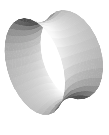
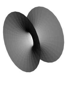
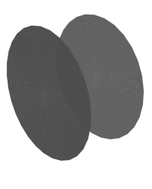
Figure 6: The three equilibrium shapes of the soap film, namely the shallow catenoid, the deep catenoid and the Goldschmidt solution, plotted at a natural scale for $L=1$.

To examine the properties of these solutions, we note that since (A.4) gives $L(0)=L(1)=0$ and $L^{\prime\prime}(u_{0})=-{2\over u_{0}(1-u_{0}^{2})^{3/2}}<0$, $L(u_{0})$ is a concave function of $u_{0}$ with a single maximum for $0\leqslant u_{0}\leqslant 1$. Setting $L^{\prime}(u_{0})=0$, we obtain the transcendental equation

$$\sqrt{1-u_{0}^{2}}\cosh^{-1}{1\over u_{0}}=1\ ,$$ (A.6)

whose solution is $u_{0{\rm c}}\simeq 0.552$ leading to the maximal length $L_{\rm c}\simeq 1.325$. We must then distinguish between two cases. For $L>L_{\rm c}$, (A.4) has no solution for $u_{0}$ and the catenoid solution does not exist at all, leaving the Goldschmidt solution as the only available one. For $L<L_{\rm c}$, on the other hand, (A.4) has two solutions for $u_{0}$, the largest (smallest) of which corresponds to a “shallow” (“deep”) catenoid. Meanwhile, the Goldschmidt solution exists as well, giving a total of three available solutions, shown in Fig. 6. To examine which one is energetically favored, we need to compare the energy of the shallow catenoid, $E(u_{0})$ with $u_{0}>u_{0{\rm c}}$, with that of the Goldschmidt solution, $E=2\pi$. The former is a decreasing function of $u_{0}$, becoming equal to $2\pi$ at $u_{0}=\tilde{u}_{0{\rm c}}\simeq 0.826$ where the separation is $\tilde{L}_{\rm c}\simeq 1.055$, and hence the lowest-energy solution is the shallow catenoid for $u_{0}>\tilde{u}_{0{\rm c}}$ and the Goldschmidt solution for $u_{0}<\tilde{u}_{0{\rm c}}$. To summarize, for $L>L_{\rm c}$ the only possible solution is the Goldschmidt solution, while for $L<L_{\rm c}$ all three solutions are available with the shallow catenoid being favored for $L<\tilde{L}_{\rm c}$ and the Goldschmidt solution being favored for $L>\tilde{L}_{\rm c}$. This behavior is shown in Fig. 7.

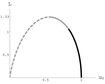
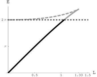
(a)	(b)

Figure 7: Plots of $L(u_{0})$ and $E(L)$, with the solid dark, solid gray and dashed gray lines corresponding to stable, metastable and unstable catenoid solutions. In the plot of $E(L)$, the dotted line corresponds to the Goldschmidt solution.

By now, the analogy with the Wilson-loop calculations in the main part of the paper should be obvious. Namely, the quantities $u_{0}$, $L$ and $E$ correspond to the quantities denoted by the same symbols in the Wilson-loop context, the shallow catenoid, deep catenoid and the Goldschmidt solution correspond to the short string, the long string and the unbound configuration respectively and the critical values $L_{\rm c}$ and $\tilde{L}_{\rm c}$ of the separation correspond to the maximal and screening lengths respectively. Fig. 7(b) in particular is qualitatively similar to Figs. 1(b) and 4(b) in the main part of the paper.

To examine the stability of the catenoid solutions, we need to consider small fluctuations about these equilibrium surfaces. In [27], the stability analysis was carried out for perturbations normal to the surface. Here, we consider the most general type of perturbation, which we parametrize as follows. Writing the equilibrium surface as $F(r,z)=r-r_{\rm cl}(z)=0$, where $r_{\rm cl}(z)=u_{0}\cosh(z/u_{0})$ is the classical solution, the unit normal to the surface is $\hat{n}={\nabla F\over|\nabla F|}$, while the unit tangent vectors along and perpendicular to the azimuthal direction are $\hat{\phi}$ and $\hat{\xi}=\hat{n}\times\hat{\phi}$, respectively. Explicitly, we have the following transformation between the two orthonormal frames with basis vectors $(\hat{n},\hat{\xi},\hat{\phi})$ and $(\hat{r},\hat{z},\hat{\phi})$, respectively

$$\hat{n}={\hat{r}-r_{\rm cl}^{\prime}\hat{z}\over\sqrt{1+r_{\rm cl}^{\prime 2}}}\ ,\qquad\hat{\xi}={\hat{z}+r_{\rm cl}^{\prime}\hat{r}\over\sqrt{1+r_{\rm cl}^{\prime 2}}}\ .$$ (A.7)

Expressing the most general perturbation as

$$\delta{\vec{r}}=\delta n\hat{n}+r\delta\phi\hat{\phi}+\delta\xi\hat{\xi}=\delta r\hat{r}+r\delta\phi\hat{\phi}+\delta z\hat{z}\ ,$$ (A.8)

we have, in terms of our original variables,

$$z = \sigma_{1}+{\delta\xi(t,\sigma_{1},\sigma_{2})-r^{\prime}_{\rm cl}(\sigma_{1})\delta n(t,\sigma_{1},\sigma_{2})\over\sqrt{1+r^{\prime 2}_{\rm cl}(\sigma_{1})}}\ ,$$

$$r = r_{\rm cl}(\sigma_{1})+{\delta n(t,\sigma_{1},\sigma_{2})+r^{\prime}_{\rm cl}(\sigma_{1})\delta\xi(t,\sigma_{1},\sigma_{2})\over\sqrt{1+r^{\prime 2}_{\rm cl}(\sigma_{1})}}\ ,$$ (A.9)

$$\phi = \sigma_{2}+\delta\phi(t,\sigma_{1},\sigma_{2})\ ,$$

From this form we can see that this is an $SO(2)$ transformation with rotation angle related to the variable $\sigma_{1}$ as $\cos\theta=1/\cosh(z/u_{0})$. Since this is local in space and global in time the kinetic energy remains diagonal in this new basis. Substituting in the original action (A.1) and expanding in powers of the perturbations, we find that the zeroth-order term gives the classical action, the first-order term vanishes by the equations of motion and periodicity of $\delta\phi$ in $\sigma_{2}$, and the second-order term reads

$$S_{2} = -{1\over u_{0}}\int dt\int d\sigma_{1}d\sigma_{2}\biggl{\{}{1\over 2}[u_{0}^{2}(\partial_{1}\delta n)^{2}+(\partial_{2}\delta n)^{2}]$$ (A.10)

$$\qquad\qquad\qquad\qquad-\>{u_{0}^{2}\over 2}\cosh^{2}{\sigma_{1}\over u_{0}}\left(\delta\dot{n}^{2}+\delta\dot{\xi}^{2}+u_{0}^{2}\cosh^{2}{\sigma_{1}\over u_{0}}\delta\dot{\phi}^{2}\right)$$

$$\qquad\qquad\qquad\qquad-\>{1\over\cosh^{2}{\sigma_{1}\over u_{0}}}\left(\delta n^{2}-{1\over 2}\delta\xi^{2}+\sinh{\sigma_{1}\over u_{0}}\delta n\delta\xi\right)$$

$$\qquad\qquad\qquad\qquad+\>{u_{0}\over\cosh{\sigma_{1}\over u_{0}}}\left[\partial_{1}(\delta n\delta\xi)+\sinh{\sigma_{1}\over u_{0}}\left({1\over 2}\partial_{1}\delta\xi^{2}+\cosh{\sigma_{1}\over u_{0}}\delta\xi\partial_{2}\delta\phi\right)\right]$$

$$\qquad\qquad\qquad\qquad+\>u_{0}^{2}\cosh{\sigma_{1}\over u_{0}}(\partial_{1}\delta\xi\partial_{2}\delta\phi-\partial_{2}\delta\xi\partial_{1}\delta\phi)\biggr{\}}\ .$$

Although the various perturbations appear to be coupled, the calculation of the equations of motion reveals that they actually decouple due to an extensive cancellation of terms. For the tangential perturbations, the equations of motion are just

$$\delta\ddot{\xi}=\delta\ddot{\phi}=0\ .$$ (A.11)

For the normal perturbations, we rename $(\sigma_{1},\sigma_{2})\to(z,\phi)$, we define $u={z\over u_{0}}$, we separate variables according to

$$\delta n(t,u,\phi)=\Phi(u)e^{-{\rm i}\Omega t}e^{{\rm i}m\phi}\ ,$$ (A.12)

and we end up with the Sturm–Liouville equation (3.7) with

$$p=1\ ,\qquad r={2\over\cosh^{2}u}-m^{2}\ ,\qquad q=\cosh^{2}u\ ,\qquad\omega=u_{0}\Omega\ ,$$ (A.13)

subject to the following boundary conditions at the endpoints

$$\Phi\left(\pm{L\over 2u_{0}}\right)=\Phi\left(\pm\cosh^{-1}{1\over u_{0}}\right)=0\ ,$$ (A.14)

where we have used (A.4). To investigate the stability of the catenoid solutions, we want to determine the sign of $\omega^{2}$ for the lowest-energy solution to the differential equation (3.7) with (A.13) in terms of $u_{0}$. Although the study of the evolution of $\omega^{2}$ as a function of $u_{0}$ is in general a hard task, we can obtain useful information by considering the corresponding zero-mode problem i.e. solving (3.7) with $\omega^{2}=0$. In this case, the transformation $x=\tanh u$ turns (3.7) into an associated Legendre equation with the general solution given by a linear combination of $P_{1}^{m}(\tanh u)$ and $Q_{1}^{m}(\tanh u)$, $m=0,\pm 1,\pm 2,\dots$. However, the boundary conditions (A.14) further restrict us to $m=0$, for which only the solution proportional to $Q_{1}(\tanh u)$ is acceptable. Therefore, the zero-mode solution reads

$$\Phi_{0}(u)=NQ_{1}(\tanh u)=N(1-u\tanh u)\ ,$$ (A.15)

where $N$ is a normalization constant. Imposing the boundary condition (A.14) leads then to the transcendental equation (A.6), that is, to the condition determining the point $u_{0{\rm c}}$ at which the length $L(u_{0})$ attains its maximum! Therefore, the equation of motion of the normal perturbations has a zero mode if and only if $u_{0}$ attains the value $u_{0{\rm c}}$ that marks the boundary between the deep and shallow catenoid solutions. This result tremendously simplifies our problem, as it implies that if we determine the evolution of the lowest eigenvalue as we move infinitesimally from $u_{0{\rm c}}$, we will in fact have determined its sign in the whole regions to the left and to the right of $u_{0{\rm c}}$. Again, one may appreciate the similarity with the case of longitudinal perturbations in the main part of the paper.

To carry out this investigation, it is convenient to transform the Sturm–Liouville problem to a Schrödinger one by applying the transformation (3.8) which, for our case, reads

$$x=\sinh u\ ,\qquad\Psi(x)=(1+x^{2})^{1/4}\Phi(u)\ .$$ (A.16)

This way, we obtain the Schrödinger equation (3.9) where the potential, for general values of $m$, is given by

$$V(x)={m^{2}\over x^{2}+1}-{x^{2}+6\over 4(x^{2}+1)^{2}}\ ,$$ (A.17)

and the boundary conditions at the endpoints read

$$\Psi(\pm x_{0})=0\ ,\qquad x_{0}=x_{0}(u_{0})\equiv{\sqrt{1-u_{0}^{2}}\over u_{0}}\ .$$ (A.18)

The potential is depicted in Fig. 8(a) and clearly does not support any negative energy states for $|m|\geqslant 2$, which is consistent with the discussion above. For $m=0$ it is deep enough to support one negative energy state if its size is restricted to a finite interval $x\in[-x_{0},x_{0}]$, with $x<x_{0\rm c}$. For $|m|=1$ there is no negative or zero energy state respecting the boundary conditions as we have seen, even though the potential has a negative part. In the new variables, the normalized zero-mode eigenfunction occurring for $m=0$ is

$$\Psi_{0}(x)={\sqrt{6}u_{0{\rm c}}(1-u_{0{\rm c}}^{2})^{3/4}\over(3-5u_{0{\rm c}}^{2})^{1/2}}(1+x^{2})^{1/4}\left(1-{x\over\sqrt{1+x^{2}}}\sinh^{-1}x\right)\ .$$ (A.19)

To determine the change in $\omega^{2}$ as $u_{0}$ deviates from $u_{0{\rm c}}$, we may use perturbation theory. Noting that the potential (A.17) is $u_{0}$–independent while the endpoints $\pm x_{0}$ given in (A.18) are $u_{0}$–dependent, we find that the appropriate perturbation-theory formula is

$$\delta\omega^{2}=2x_{0}^{\prime}(u_{0{\rm c}})\Psi_{0}^{2}(x_{0\rm c})V(x_{0\rm c})\ \delta u_{0}\ ,$$ (A.20)

as is read off from (3.33), appropriately adapted to a Schrödinger problem for a real wavefunction in the range $[-x_{0\rm c},x_{0\rm c}]$ and with the boundary condition in (A.18). In our case $x_{0\rm c}\simeq 1.509$.

​​​​	​​​​ ​​​​	​​​​ ​​​​
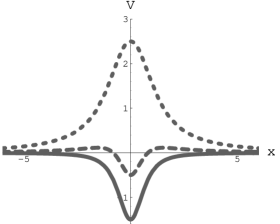
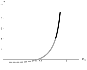
​​​(a)	(b)	​​​​​(c)

Figure 8: (a) Schrödinger potentials for the normal perturbations with angular quantum numbers $m=0$ (solid), $m=\pm 1$ (dashed) and $m=\pm 2$ (dotted). (b) Evolution of the lowest eigenvalue $\omega^{2}$ with $u_{0}$, calculated using the shooting method and Mathematica’s [28] NDSolve routine. The slope of the curve at $u_{0}=u_{0{\rm c}}$ is found to be $4.497$, in perfect agreement with (A.21). (c) Plots of the normalized ground-state wavefunction $\Psi_{0}(x)$ for $u_{0}=0.8>u_{0{\rm c}}$ (solid) and $u_{0}=0.3<u_{0{\rm c}}$ (dashed).

To calculate $\delta\omega^{2}$, we insert (A.17) and (A.19) into (A.20), making repeated use of (A.6) to simplify the resulting expressions. When the smoke clears out, we find

$$\delta\omega^{2}={12u_{0\rm c}\over 3-5u_{0\rm c}^{2}}\delta u_{0}\simeq 4.497\ \delta u_{0}\ .$$ (A.21)

Hence, as we move to the right (left) of $u_{0{\rm c}}$, the eigenvalue $\omega^{2}$ becomes positive (negative) and therefore the shallow catenoid is stable while the deep catenoid is unstable, as expected. This behavior is confirmed by a numerical analysis, shown in Fig. 8.

References

- [1]
- [2] J.M. Maldacena, Adv. Theor. Math. Phys. 2 (1998) 231, Int. J. Theor. Phys. 38 (1999) 1113, hep-th/9711200. S.S. Gubser, I.R. Klebanov and A.M. Polyakov, Phys. Lett. B428 (1998) 105, hep-th/9802109. E. Witten, Adv. Theor. Math. Phys. 2 (1998) 253, hep-th/9802150 and Adv. Theor. Math. Phys. 2 (1998) 505, hep-th/9803131.
- [3] J.M. Maldacena, Phys. Rev. Lett. 80 (1998) 4859, hep-th/9803002. S.J. Rey and J.T. Yee, Eur. Phys. J. C22 (2001) 379, hep-th/9803001.
- [4] S.J. Rey, S. Theisen and J.T. Yee, Nucl. Phys. B527 (1998) 171, hep-th/9803135. A. Brandhuber, N. Itzhaki, J. Sonnenschein and S. Yankielowicz, Phys. Lett. B434 (1998) 36, hep-th/9803137 and JHEP 9806 (1998) 001, hep-th/9803263.
- [5] A. Brandhuber and K. Sfetsos, Adv. Theor. Math. Phys. 3 (1999) 851, hep-th/9906201.
- [6] K. Peeters, J. Sonnenschein and M. Zamaklar, Phys. Rev. D74 (2006) 106008, hep-th/0606195.
- [7] H. Liu, K. Rajagopal and U.A. Wiedemann, An AdS/CFT calculation of screening in a hot wind, hep-ph/0607062.
- [8] M. Chernicoff, J.A. Garcia and A. Guijosa, JHEP 0609 (2006) 068, hep-th/0607089.
- [9] S.D. Avramis, K. Sfetsos and D. Zoakos, Phys. Rev. D75 (2007) 025009, hep-th/0609079.
- [10] P.C. Argyres, M. Edalati and J.F. Vázquez-Poritz, JHEP 0701 (2007) 105, hep-th/0608118.
- [11] C.G. Callan and A. Guijosa, Nucl. Phys. B565 (2000) 157, hep-th/9906153.
- [12] I.R. Klebanov, J.M. Maldacena and C.B. Thorn, JHEP 0604 (2006) 024, hep-th/0602255.
- [13] J.J. Friess, S.S. Gubser, G. Michalogiorgakis and S.S. Pufu, Stability of strings binding heavy-quark mesons, hep-th/0609137.
- [14] S.D. Avramis and K. Sfetsos, JHEP 0701 (2007) 065, hep-th/0606190.
- [15] B. Baumgartner, H. Grosse and A. Martin, Nucl. Phys. B254 (1985) 528. C. Bachas, Phys. Rev. D33 (1986) 2723.
- [16] Y. Kinar, E. Schreiber, J. Sonnenschein and N. Weiss, Nucl. Phys. B583 (2000) 76, hep-th/9911123.
- [17] M. Cvetic and D. Youm, Nucl. Phys. B477 (1996) 449, hep-th/9605051.
- [18] J.G. Russo and K. Sfetsos, Adv. Theor. Math. Phys. 3 (1999) 131, hep-th/9901056.
- [19] P. Kraus, F. Larsen and S.P. Trivedi, JHEP 9903 (1999) 003, hep-th/9811120.
- [20] K. Sfetsos, JHEP 9901 (1999) 015, hep-th/9811167.
- [21] I. Bakas and K. Sfetsos, Nucl. Phys. B573 (2000) 768, hep-th/9909041. I. Bakas, A. Brandhuber and K. Sfetsos, Adv. Theor. Math. Phys. 3 (1999) 1657, hep-th/9912132. M. Cvetic, S. S. Gubser, H. Lu and C. N. Pope, Phys. Rev. D62 (2000) 086003, hep-th/9909121.
- [22] D.Z. Freedman, S.S. Gubser, K. Pilch and N.P. Warner, JHEP 0007 (2000) 038, hep-th/9906194.
- [23] R. Hernández, K. Sfetsos and D. Zoakos, JHEP 0603, 069 (2006), hep-th/0510132 and Fortsch. Phys. 54, 407 (2006), hep-th/0512158.
- [24] C. Ahn and J.F. Vázquez-Poritz, JHEP 0606 (2006) 061, hep-th/0603142.
- [25] D.J. Gross and H. Ooguri, Phys. Rev. D58 (1998) 106002, hep-th/9805129.
- [26] C. Caratheodory, Calculus of Variations and Partial Differential Equations of the First Order, American Mathematical Society, 1999. G.A. Bliss, Calculus of Variations, Chicago, IL: Open Court, 1925. R. Courant and H. Robbins, What is Mathematics?, Oxford University Press, Oxford, 1941. G.B. Arfken and H.J. Weber, Mathematical Methods for Physicists, 6th edition, Elsevier Academic Press.
- [27] L. Durand, Am. J. Phys. 49 (1981) 334.
- [28] S. Wolfram, Mathematica Version 5.0, Wolfram Research, 1988-2003.