Baryonic Condensates on the Conifold

Abstract

We provide new evidence for the gauge/string duality between the baryonic branch of the cascading $SU(k(M+1))\times SU(kM)$ gauge theory and a family of type IIB flux backgrounds based on warped products of the deformed conifold and $\mathbb{R}^{3,1}$. We show that a Euclidean D5-brane wrapping all six deformed conifold directions can be used to measure the baryon expectation values, and present arguments based on $\kappa$-symmetry and the equations of motion that identify the gauge bundles required to ensure worldvolume supersymmetry of this object. Furthermore, we investigate its coupling to the pseudoscalar and scalar modes associated with the phase and magnitude, respectively, of the baryon expectation value. We find that these massless modes perturb the Dirac-Born-Infeld and Chern-Simons terms of the D5-brane action in a way consistent with our identification of the baryonic condensates. We match the scaling dimension of the baryon operators computed from the D5-brane action with that found in the cascading gauge theory. We also derive and numerically evaluate an expression that describes the variation of the baryon expectation values along the supergravity dual of the baryonic branch.

Department of Physics and Princeton Center for Theoretical Physics,
Princeton University, Princeton, NJ 08544

1 Introduction

Consideration of a stack of $N$ D3-branes leads to the conjectured duality of $\mathcal{N}=4$ super Yang-Mills theory to type IIB string theory on $AdS_{5}\times S^{5}$ [1, 2, 3]. A different, $\mathcal{N}=1$ supersymmetric example of the AdS/CFT correspondence follows from placing the stack of D3-branes at the tip of the conifold [4, 5]. This suggests a duality between a certain $SU(N)\times SU(N)$ superconformal gauge theory and type IIB string theory on $AdS_{5}\times T^{1,1}$. Addition of $M$ D5-branes wrapped over the two-sphere near the tip of the conifold changes the gauge group to $SU(N+M)\times SU(N)$ [6, 7]. This theory is non-conformal; it undergoes a cascade of Seiberg dualities [8] $\mathrm{SU}(N+M)\times\mathrm{SU}(N)\rightarrow\mathrm{SU}(N-M)\times\mathrm{SU}(N)$ as it flows from the UV to the IR [9, 10] (for reviews, see [11, 12]).

The gauge theory contains two doublets of bifundamental, chiral superfields $A_{i},B_{j}$ (with $i,j=1,2$). In the conformal case, $M=0$, it has continuous global symmetries $\mathrm{SU}(2)_{A}\times\mathrm{SU}(2)_{B}\times\mathrm{U}(1)_{R}\times\mathrm{U}(1)_{B}$. The two $\mathrm{SU}(2)$ groups rotate the doublets $A_{i}$ and $B_{j}$, while one $\mathrm{U}(1)$ is an R-symmetry. The remaining $\mathrm{U}(1)$ factor corresponds to the baryon number symmetry which we will be most interested in. As argued in [10, 13, 14, 15], in the cascading theory where $N$ is an integer multiple of $M$, $N=kM$, this symmetry is spontaneously broken by condensates of baryonic operators. In this paper we will provide a quantitative verification of this effect.

For $N=kM$ the last step of the cascade is an $\mathrm{SU}(2M)\times\mathrm{SU}(M)$ theory which admits two baryon operators (sometimes referred to as baryon and antibaryon)

$$\mathcal{A} \sim \epsilon_{\alpha_{1}\alpha_{2}\ldots\alpha_{2M}}(A_{1})_{1}^{\alpha_{1}}(A_{1})_{2}^{\alpha_{2}}\ldots(A_{1})_{M}^{\alpha_{M}}(A_{2})_{1}^{\alpha_{M+1}}(A_{2})_{2}^{\alpha_{M+2}}\ldots(A_{1})_{M}^{\alpha_{2M}}\ ,$$

$$\mathcal{B} \sim \epsilon_{\alpha_{1}\alpha_{2}\ldots\alpha_{2M}}(B_{1})_{1}^{\alpha_{1}}(B_{1})_{2}^{\alpha_{2}}\ldots(B_{1})_{M}^{\alpha_{M}}(B_{2})_{1}^{\alpha_{M+1}}(B_{2})_{2}^{\alpha_{M+2}}\ldots(B_{1})_{M}^{\alpha_{2M}}\ .\qquad$$ (1)

Baryon operators of the general $\mathrm{SU}(M(k+1))\times\mathrm{SU}(Mk)$ theory have the schematic form $(A_{1}A_{2})^{k(k+1)M/2}$ and $(B_{1}B_{2})^{k(k+1)M/2}$, with appropriate contractions described in [13]. Unlike the “dibaryon” operators of the conformal $\mathrm{SU}(N)\times\mathrm{SU}(N)$ theory [6], $\mathcal{A}$ and $\mathcal{B}$ are singlets under the two global $\mathrm{SU}(2)$ symmetries. These operators acquire expectation values that spontaneously break the $\mathrm{U}(1)_{B}$ baryon number symmetry; this is why the gauge theory is said to be on the baryonic branch of its moduli space [16]. Supersymmetric vacua on the one complex dimensional baryonic branch are subject to the constraint $\mathcal{A}\mathcal{B}=-\Lambda^{4M}_{2M}$, and thus we can parameterize it as follows

$$\mathcal{A}=i\zeta\Lambda^{2M}_{2M}\ ,\qquad\mathcal{B}=\frac{i}{\zeta}\Lambda^{2M}_{2M}\ .$$ (2)

The non-singular supergravity dual of the theory with $|\zeta|=1$ is the warped deformed conifold found in [10]. In [14] the linearized scalar and pseudoscalar perturbations, corresponding to small deviations of $\zeta$ from $1$, were constructed. The full set of first-order equations necessary to describe the entire moduli space of supergravity backgrounds dual to the baryonic branch, sometimes called the resolved warped deformed conifolds, was derived and solved numerically in [17] (for a further discussion of the solutions, see [15]).

The construction of this moduli space of supergravity backgrounds, which have just the right symmetries to be identified with the baryonic branch in the cascading gauge theory, provides an excellent check on the gauge/string duality in this intricate setting. Yet, one question remains: how do we identify the baryonic expectation values on the string side of this duality? Among other things, this is needed to construct a map between the parameter $U$ that labels the supergravity solutions, and the parameter $|\zeta|$ in the gauge theory.

The dual string theory description of the baryon operators (1) was first considered by Aharony [13]. He argued that the heavy “particle” dual to such an operator is described at large $r$ by a D5-brane wrapped over the $T^{1,1}$, with some D3-branes dissolved in it (to account for this, the world volume gauge field needs to be turned on). To calculate the two-point function of baryon operators inserted at $x_{1}$ and $x_{2}$ we may use a semi-classical approach to the AdS/CFT correspondence. Then we need a (Euclidean) D5-brane whose world volume has two $T^{1,1}$ boundaries at large $r$, located at $x_{1}$ and $x_{2}$. In this paper we will be interested in a simpler embedding of the D5-brane: as suggested by Witten [18], the object needed to calculate the baryonic expectation values is the Euclidean D5-brane that has the appearance of a pointlike instanton from the four-dimensional point of view, and wraps the remaining six (generalized Calabi-Yau) directions of the ten-dimensional spacetime. This object has a single $T^{1,1}$ boundary at large $r$, corresponding to insertion of just one baryon operator. As we will find, supersymmetry requires that the world volume gauge field is also turned on, so there are D3-branes dissolved in the D5. This identification will be corroborated by demonstrating that the D5-brane couples correctly to the pseudoscalar zero-mode of the theory that changes the phase of the baryon expectation value [14].

Close to the boundary, a field $\phi$ dual to an operator of dimension $\Delta$ in the AdS/CFT correspondence behaves as

$$\phi(x,r)=\phi_{0}(x)\,r^{\Delta-4}+A_{\phi}(x)\,r^{-\Delta}\ ,$$ (3)

Here $A_{\phi}$ is the operator expectation value [19], and $\phi_{0}$ is the source for it. In the cascading theory, which is near-AdS in the UV, the same formulae hold modulo powers of $\ln r$ [20, 21]. The field corresponding to a baryon will be identified, at a semi-classical level, with $e^{-S_{D5}(r)}$, where $S_{D5}(r)$ is the action of a D5-brane wrapping the Calabi-Yau coordinates up to the radial coordinate cut-off $r$. The different baryon operators ${\mathcal{A}},\overline{{\mathcal{A}}},{\mathcal{B}},\overline{{\mathcal{B}}}$ will be distinguished by the two possible D5-brane orientations, and the two possible $\kappa$-symmetric choices for the world volume gauge field that has to be turned on inside the D5-brane. In the cascading gauge theory there is no source added for baryonic operators, hence we find that $\phi_{0}=0$. On the other hand, the term scaling as $r^{-\Delta}$ is indeed revealed by our calculation of $e^{-S_{D5}(r)}$ as a function of the radial cut-off, allowing us to find the dimensions of the baryon operators, and the values of their condensates.

This paper is structured as follows. In the remainder of section 1 we review the geometry of the deformed conifold, and the warped supergravity backgrounds dual to the baryonic branch, including the corresponding Killing spinors. We also review the $\kappa$-symmetry conditions for D-brane embeddings, and briefly discuss a number of brane configurations that satisfy them. Section 2 is devoted to the derivation of the first-order equation for the gauge field. We first discuss a Lorentzian D7-brane wrapping the warped deformed conifold directions, before presenting a parallel treatment for the more subtle case of the Euclidean D5-brane wrapping the conifold. Section 3 is devoted to the physics of the D5-instanton in the KS background. From the behavior of the D5-brane action as a function of the radial cut-off we extract the dimension of the baryon operator, and show that it matches the expectations from the dual cascading gauge theory. We also show that the D5-brane couples to the baryonic branch complex modulus in the way consistent with our identification of the condensates. In particular, we demonstrate that pseudoscalar perturbations of the backgrounds shift the phase of the baryon expectation value. We generalize to the complete baryonic branch in section 4 where we compute the baryon expectation values as a function of the supergravity modulus $U$. The product of the expectation values calculated from the D5-brane action is shown to be independent of $U$ in agreement with (2). Finally, we present an integral expression for their ratio and evaluate it numerically, which provides a relation between the baryonic branch modulus $|\zeta|$ in the gauge theory and the modulus $U$ in the dual supergravity description, and show that they satisfy $\mathcal{A}\mathcal{B}={\rm const}$. We conclude briefly in section 5.

1.1 Review of Warped Deformed Conifolds

We start our discussion with a review of the warped deformed conifold (KS) background [10], which is dual to a locus on the baryonic branch where $|{\cal A}|=|{\cal B}|$. Then we review the generalization of the background to the entire baryonic branch found by Butti et. al. [17].

The warped deformed conifold is a warped product of four-dimensional flat space and an $SU(2)\times SU(2)$ Calabi-Yau three-fold $\mathcal{M}$:

$$ds^{2}=h(t)^{-1/2}dx_{3,1}^{2}+h(t)^{1/2}ds_{\mathcal{M}}^{2}\ .$$ (4)

The deformed conifold $\mathcal{M}$ is described in complex coordinates by the equation

$$\sum_{i=1}^{4}z_{i}^{2}=\varepsilon^{2}\ .$$ (5)

The warp factor is given by

$$h(t) = (g_{s}M\alpha^{\prime})^{2}2^{2/3}\varepsilon^{-8/3}I(t)\ ,$$ (6)

$$I(t) \equiv 2^{1/3}\int_{t}^{\infty}dx\frac{x\coth(x)-1}{\sinh^{2}(x)}(\sinh(x)\cosh(x)-x)^{1/3}\ ,$$ (7)

In the asymptotic near-AdS region, the radial coordinate $t$ is related to the standard coordinate $r$ by

$$r^{2}=\frac{3}{2^{5/3}}\varepsilon^{4/3}e^{2\,t/3}\ .$$ (8)

Since $\mathcal{M}$ has a topology of $S^{2}\times S^{3}\times\mathbb{R}^{+}$ it is convenient to introduce the following one-forms $e_{i}$ on $S^{2}$

$$e_{1}\equiv d\theta_{1}\ ,\qquad e_{2}\equiv-\sin\theta_{1}d\phi_{1}\ ,$$ (9)

and a set of invariant forms on $S^{3}$

$$\epsilon_{1} \equiv \sin\psi\sin\theta_{2}d\phi_{2}+\cos\psi d\theta_{2}\ ,$$ (10)

$$\epsilon_{2} \equiv \cos\psi\sin\theta_{2}d\phi_{2}-\sin\psi d\theta_{2}\ ,$$ (11)

$$\epsilon_{3} \equiv d\psi+\cos\theta_{2}d\phi_{2}\ .$$ (12)

In term of these we define one-forms

$$g_{1} \equiv {e_{2}-\epsilon_{2}\over\sqrt{2}}\ ,\quad g_{2}\equiv{e_{1}-\epsilon_{1}\over\sqrt{2}}\ ,$$ (13)

$$g_{3} \equiv {e_{2}+\epsilon_{2}\over\sqrt{2}}\ ,\quad g_{4}\equiv{e_{1}+\epsilon_{1}\over\sqrt{2}}\ ,$$ (14)

$$g_{5} \equiv \epsilon_{3}+\cos\theta_{1}d\phi_{1}\ ,$$ (15)

which allow for a concise description of the Calabi-Yau metric on $\mathcal{M}$:

$$ds^{2}_{\mathcal{M}}={\varepsilon^{4/3}K(t)\over 2}\left[\sinh^{2}\left({t\over 2}\right)\left(g_{1}^{2}+g_{2}^{2}\right)+\cosh^{2}\left({t\over 2}\right)\left(g_{3}^{2}+g_{4}^{2}\right)+{1\over 3K(t)^{3}}\left(dt^{2}+g_{5}^{2}\right)\right]\ ,$$ (16)

where

$$K(t)\equiv{\left(\sinh(t)\cosh(t)-t\right)^{1/3}\over\sinh(t)}\ .$$ (17)

The dilaton $\phi$ is constant, but there are non-trivial three- and five-form fluxes in this background [10]. The NS-NS two-form is given by

$$B_{2}=\frac{g_{s}M\alpha^{\prime}}{2}\frac{t\coth(t)-1}{\sinh(t)}\left[\sinh^{2}\left(\frac{t}{2}\right)\,g^{1}\wedge g^{2}+\cosh^{2}\left(\frac{t}{2}\right)\,g^{3}\wedge g^{4}\right],$$ (18)

and the R-R fluxes are most compactly written as

$$F_{3} = \frac{M\alpha^{\prime}}{2}\left\{g^{3}\wedge g^{4}\wedge g^{5}+d\left[\frac{\sinh(t)-t}{2\sinh(t)}(g^{1}\wedge g^{3}+g^{2}\wedge g^{4})\right]\right\},$$ (19)

$$\tilde{F}_{5} = dC_{4}+B_{2}\wedge F_{3}=(1+\ast)\,(B_{2}\wedge F_{3})\ .$$ (20)

Corresponding R-R potentials are easily found:

$$C_{2} = \frac{M\alpha^{\prime}}{2}\big{[}\frac{\psi}{2}(g^{1}\wedge g^{2}+g^{3}\wedge g^{4})-\frac{1}{2}\cos\theta_{1}\cos\theta_{2}\,d\phi_{1}\wedge d\phi_{2}$$ (21)

$$\qquad\quad-\frac{t}{2\sinh(t)}(g^{1}\wedge g^{3}+g^{2}\wedge g^{4})\big{]}\ ,$$

$$C_{4} = \frac{1}{g_{s}h(t)}\,dx^{0}\wedge dx^{1}\wedge dx^{2}\wedge dx^{3}\ .$$ (22)

From here on we set the deformation parameter $\varepsilon$ to unity for notational simplicity, and also choose $M\alpha^{\prime}=2$ and $g_{s}=1$.

The KS solution is invariant under the $\mathbb{Z}_{2}$ symmetry ${\cal I}$, which exchanges $(\theta_{1},\phi_{1})$ with $(\theta_{2},\phi_{2})$ accompanied by the action of $-I$ of SL(2, $\mathbb{Z}$). On the gauge theory side, this symmetry exchanges the $\mathcal{A}$ and $\mathcal{B}$ baryons. Therefore, the KS solution corresponds to $|\zeta|=1$ in (2). There is a continuous family of solutions which generalize KS and break this ${\cal I}$–symmetry [14, 17]. This family is dual to the entire baryonic branch of the cascading gauge theory, parameterized by $\zeta$ (only the modulus of $\zeta$ is manifest in these backgrounds). The corresponding metric can be written in the form of the Papadopoulos-Tseytlin ansatz [22] in the string frame:

$$ds^{2}=e^{2A}dx^{2}_{3,1}+e^{x}ds_{\mathcal{M}}^{2}=e^{2A}dx^{2}_{3,1}+\sum_{i=1}^{6}G_{i}^{2}\ ,$$ (23)

where

$$G_{1}\equiv e^{(x+g)/2}\,e_{1}\ , \qquad G_{2}\equiv{\cosh(t)+a\over\sinh(t)}\,e^{(x+g)/2}\,e_{2}+{e^{g}\over\sinh(t)}\,e^{(x-g)/2}\,(\epsilon_{2}-ae_{2})\ ,$$

$$G_{3}\equiv e^{(x-g)/2}\,(\epsilon_{1}-ae_{1})\ , \qquad G_{4}\equiv{e^{g}\over\sinh(t)}\,e^{(x+g)/2}\,e_{2}-{\cosh(t)+a\over\sinh(t)}\,e^{(x-g)/2}\,(\epsilon_{2}-ae_{2})\ ,$$

$$G_{5}\equiv e^{x/2}\,v^{-1/2}dt\ , \qquad G_{6}\equiv e^{x/2}\,v^{-1/2}g_{5}\ .$$ (24)

While in the KS case there was a single warp factor $h(t)$, now we find several functions $A(t),x(t),g(t),a(t),v(t)$.

In terms of these one-forms the Calabi-Yau $(3,0)$ form is

$$\Omega=(G_{1}+iG_{2})\wedge(G_{3}+iG_{4})\wedge(G_{5}+iG_{6})\ ,$$ (25)

and the fundamental $(1,1)$ form is

$$J={i\over 2}\Big{[}(G_{1}+iG_{2})\wedge(G_{1}-iG_{2})+(G_{3}+iG_{4})\wedge(G_{3}-iG_{4})+(G_{5}+iG_{6})\wedge(G_{5}-iG_{6})\Big{]}\ .$$ (26)

The background also contains the fluxes

$$B_{2} = h_{1}\,(\epsilon_{1}\wedge\epsilon_{2}+e_{1}\wedge e_{2})+\chi\,(e_{1}\wedge e_{2}-\epsilon_{1}\wedge\epsilon_{2})+h_{2}\,(\epsilon_{1}\wedge e_{2}-\epsilon_{2}\wedge e_{1})\ ,$$

$$F_{3} = -{1\over 2}g_{5}\wedge\big{[}\epsilon_{1}\wedge\epsilon_{2}+e_{1}\wedge e_{2}-b\,(\epsilon_{1}\wedge e_{2}-\epsilon_{2}\wedge e_{1})\big{]}-{1\over 2}\,dt\wedge\big{[}b^{\prime}\,(\epsilon_{1}\wedge e_{1}+\epsilon_{2}\wedge e_{2})\big{]}\ ,$$

$$\tilde{F}_{5} = {\cal F}_{5}+*_{10}{\cal F}_{5}\ ,\qquad{\cal F}_{5}=-(h_{1}+bh_{2})\,e_{1}\wedge e_{2}\wedge\epsilon_{1}\wedge\epsilon_{2}\wedge\epsilon_{3}\ ,$$ (27)

parameterized by functions $h_{1}(t),h_{2}(t),b(t)$ and $\chi(t)$. In addition, the dilaton $\phi$ now also depends on the radial coordinate $t$.

The functions $a$ and $v$ satisfy a system of coupled first order differential equations [17] whose solutions are known in closed form only in the KS [10] and the Chamseddine-Volkov-Maldacena-Nunez (CVMN) [23, 24] limits. All other functions $A,x,g,h_{1},h_{2},b,\chi,\phi$ are unambiguously determined by $a$ and $v$ through the relations

$$e^{-4A}=U^{-2}\left(e^{-2\phi}-1\right)\ , \qquad e^{2x}={(bC-1)^{2}\over 4(aC-1)^{2}}e^{2g+2\phi}(1-e^{2\phi})\ ,$$ (28)

$$e^{2g}=-1-a^{2}+2a\,C\ , \qquad h_{1}=-h_{2}\,C\ ,$$ (29)

$$h_{2}={e^{2\phi}(bC-1)\over 2S}\ , \qquad b={t\over S}\ ,$$ (30)

$$\chi^{\prime}=a(b-C)(aC-1)e^{2(\phi-g)}\ , \qquad\phi^{\prime}={\left(C-b\right){\left(a\,C-1\right)}^{2}\over\left(b\,C-1\right)S}\,e^{-2\,g}\ ,$$ (31)

where $C\equiv-\cosh(t),\ S\equiv-\sinh(t)$, and we remind the reader that we set ${M\alpha^{\prime}/2}=\varepsilon=g_{s}=1$, and require $\phi(\infty)=0$. In writing these equations we have specialized to the baryonic branch by imposing appropriate boundary conditions at infinity [15]; namely $\eta=1$ in the notation of [17]. Varying $\eta$ produces a more general, two parameter family of SU(3) structure backgrounds, that also include the CVMN solution [23, 24], which requires $\eta=0$ [17]. The baryonic branch ($\eta=1$) family of supergravity solutions is labelled by one real “resolution parameter” $U$ [15]. While the leading asymptotics of all supergravity backgrounds dual to the baryonic branch are given by the KT solution [9], terms subleading at large $t$ depend on $U$. This family of supergravity solutions preserves the $SU(2)\times SU(2)$ symmetry, but for $U\neq 0$ breaks the $\mathbb{Z}_{2}$ symmetry ${\cal I}$ of the KS background.

On the baryonic branch we can consider a transformation that takes $\zeta$ into $\zeta^{-1}$, or equivalently $U$ into $-U$. This transformation leaves $v$ invariant and changes $a$ as follows

$$a\rightarrow-{a\over 1+2a\cosh(t)}\ .$$ (32)

It is straightforward to check that $ae^{-g}$ is invariant while $(1+a\cosh(t))e^{-g}$ changes sign. This transformation also exchanges $e^{g}+a^{2}e^{-g}$ with $e^{-g}$ and therefore it is equivalent to the exchange of $(\theta_{1},\phi_{1})$ and $(\theta_{2},\phi_{2})$ involved in the ${\cal I}$–symmetry.

1.2 D-Branes, $\kappa$-Symmetry and Killing Spinors of the Conifold

A Dirichlet $p$-brane (with $p$ spatially extended dimensions) in string theory is described by an action consisting of two terms [25, 26, 27]: the Dirac-Born-Infeld action, which is essentially a minimal area action including non-linear electrodynamics, and the Chern-Simons action, which describes the coupling to the R-R background fields:

$$S=S_{DBI}+S_{CS}={\bf-}\int_{\mathcal{W}}\mathrm{d}^{p+1}\sigma e^{-\phi}\sqrt{-\det(G+\mathcal{F})}+\int_{\mathcal{W}}e^{\mathcal{F}}\wedge C\ .$$ (33)

Here $\mathcal{W}$ is the worldvolume of the brane and we have set the brane tension to unity. Further, $G$ is the induced metric on the worldvolume, $\mathcal{F}=F_{2}+B_{2}$ is the sum of the gauge field strength $F_{2}=dA_{1}$ and the pullback of the NS-NS two-form field, and $C=\sum_{i}C_{i}$ is the formal sum of the R-R potentials. In superstring theory all these fields should really be understood as superfields, but we shall ignore fermionic excitations here.

Wick rotation of this action to Euclidian space such that all $p+1$ directions become spatially extended (which leads to a Euclidean worldvolume D-instanton) effectively multiplies the action by a factor of $i$. This cancels the minus sign under the square root in the DBI term and leaves it real since the determinant is now positive. The CS term however is purely imaginary now. Consequently the equations of motion that follow from the DBI and CS terms now have be satisfied independently of each other if we insist on the gauge field being real.

The action (33) is invariant on shell under the so-called $\kappa$-symmetry [28, 29, 30]. This allows us to find first-order equations for supersymmetric configurations which are easier to solve than the second order equations of motion. The $\kappa$-symmetry condition can be written as

$$\Gamma_{\kappa}\epsilon=\epsilon\ ,$$ (34)

where $\epsilon$ is a doublet of Majorana-Weyl spinors, and the operator $\Gamma_{\kappa}$ is specified below. Satisfying this equation guarantees worldvolume supersymmetry in the probe brane approximation, and every solution for which $\epsilon$ is a Killing spinor corresponds to a supersymmetry compatible with those preserved by the background.

The decomposition of a Weyl spinor $\epsilon$ into a doublet of Majorana-Weyl spinors

$$\epsilon=\left(\begin{array}[]{c}\epsilon_{1}\\ \epsilon_{2}\\ \end{array}\right)$$ (37)

is achieved by projecting onto the eigenstates of charge conjugation $\epsilon_{1}=(\epsilon+\epsilon^{*})/2$ and $\epsilon_{2}=(\epsilon-\epsilon^{*})/2i$.

In IIB superstring theory on a $(9,1)$ signature spacetime, the $\kappa$-symmetry operator $\Gamma_{\kappa}$ for a Lorentzian D-brane extended along the time direction $x_{0}$ and $p$ spatial directions is given by

$$\Gamma_{\kappa}=\frac{\sqrt{-\det G}}{\sqrt{-\det(G+\mathcal{F})}}\sum_{n=0}^{\infty}(-1)^{n}\hskip 2.84544pt\raisebox{0.71114pt}{/}\mathcal{F}^{n}\Gamma_{(p+1)}\otimes(\sigma_{3})^{n+\frac{p-3}{2}}i\sigma_{2}\ ,$$ (38)

$$\Gamma_{(p+1)}\equiv\frac{1}{(p+1)!\sqrt{-\det G}}\,\epsilon^{\,\mu_{1}\ldots\mu_{p+1}}\Gamma_{\mu_{1}\ldots\mu_{p+1}}\ ,$$ (39)

$$\hskip 2.84544pt\raisebox{0.71114pt}{/}\mathcal{F}^{n}\equiv\frac{1}{2^{n}n!}\Gamma_{\nu_{1}\ldots\nu_{2n}}\mathcal{F}_{\sigma_{1}\sigma_{2}}\ldots\mathcal{F}_{\sigma_{2n-1}\sigma_{2n}}G^{\nu_{1}\sigma_{1}}\ldots G^{\nu_{2n}\sigma_{2n}}\ .$$ (40)

Here $\sigma_{i}$ are the usual Pauli matrices. We use Greek labels for the worldvolume indices of the D-brane and consequentially the $\Gamma_{\mu}$ are induced Dirac matrices. In what follows we denote the Minkowski spacetime coordinates by $x_{0}\ldots x_{3}$ and label the tangent space of the internal manifold $\mathcal{M}$ by $1,2\ldots 6$ in reference to the basis one-forms (1.1). The expression for $\Gamma_{\kappa}$ can be significantly simplified for an embedding covering all six directions of the deformed conifold, in which case we simply align the worldvolume tangent space with that of $\mathcal{M}$.

The Killing spinor $\Psi$ of the supergravity backgrounds dual to the baryonic branch is built out of a six-dimensional pure spinor $\eta^{-}$ and an arbitrary spinor $\zeta^{-}$ of negative four-dimensional chirality,

$$\Psi=\alpha\,\zeta^{-}\otimes\eta^{-}+i\beta\,\zeta^{+}\otimes\eta^{+}\ ,$$ (41)

$$(\Gamma_{1}-i\Gamma_{2})\zeta^{-}\otimes\eta^{-}=(\Gamma_{3}-i\Gamma_{4})\zeta^{-}\otimes\eta^{-}=(\Gamma_{5}-i\Gamma_{6})\zeta^{-}\otimes\eta^{-}=0\ ,$$ (42)

where $\eta^{+}=(\eta^{-})^{\ast}$ and $\zeta^{+}=(\zeta^{-})^{\ast}$. The functions $\alpha$ and $\beta$ are real [17, 15] and given by

$$\alpha={e^{\phi/4}(1+e^{\phi})^{3/8}\over(1-e^{\phi})^{1/8}}\ ,\qquad\beta={e^{\phi/4}(1-e^{\phi})^{3/8}\over(1+e^{\phi})^{1/8}}\ .$$ (43)

(this expression for $\beta$ is for $U>0$; $\beta$ changes sign when $U$ does). The corresponding Majorana-Weyl spinors $\Psi_{1}$ and $\Psi_{2}$ are

$$\Psi_{1}={1\over 2}\left((\alpha-i\beta)\zeta^{-}\otimes\eta^{-}+(\alpha+i\beta)\zeta^{+}\otimes\eta^{+}\right)\ ,$$ (44)

$$\Psi_{2}={1\over 2i}\left((\alpha+i\beta)\zeta^{-}\otimes\eta^{-}-(\alpha-i\beta)\zeta^{+}\otimes\eta^{+}\right)\ .$$ (45)

1.3 Branes Wrapping the Angular Directions

In the context of the conifold, the closest analogue to the baryon vertex in AdS${}_{5}\times\mathrm{S}^{5}$ that was discussed in [31, 32, 33], would be a D5-brane wrapping the five angular directions of the internal space, with worldvolume coordinates $\sigma^{\mu}=(x^{0},\theta_{1},\phi_{1},\theta_{2},\phi_{2},\psi)$. The brane describing the baryon vertex in AdS${}_{5}\times\mathrm{S}^{5}$ has “BI-on” spikes corresponding to fundamental strings attached to the brane and ending on the boundary of AdS, indicating that it is not a gauge-invariant object. Here however, we are interested in gauge-invariant, supersymmetric objects, that are candidate duals to chiral operators in the gauge theory, so we might try to consider a smooth embedding at constant radial coordinate (the difference between a “baryon” and a “baryon vertex” was already stressed in [31]).

To avoid having the BI-on spikes, it was proposed [13] that we should use an appropriate combination of D5-branes wrapping all the angular coordinates, and of D3-branes wrapping the $S^{3}$. This is equivalent to turning on a particular gauge field on the wrapped D5-brane. Unfortunately, it is not clear how to maintain the supersymmetry of such an object. It is not hard to see, for example from the appropriate $\kappa$-symmetry equations, that a (Lorentzian) D5-brane wrapping the five angular direction of the conifold and embedded at constant $r$ cannot be a supersymmetric object. The $\kappa$-symmetry equation seems to call for an additional constraint of the form $\Gamma_{x^{0}\psi}\epsilon^{\ast}=-i\epsilon$ on the Killing spinors, which would imply also $\Gamma_{x^{0}r}\epsilon^{\ast}=-\epsilon$, i.e. precisely what we would expect for strings stretched in the radial direction. However, such a projection does not commute with the other conditions that the Killing spinors have to satisfy and thus is not consistent. This was pointed out in [34] for the case of the singular conifold [4], and the argument carries over to the deformed conifold. Even with a worldvolume gauge field such a D5-brane cannot be a BPS object.

The same conclusion also follows from the equation of motion for the radial component of the embedding $X^{M}(\zeta^{\mu})$. The leading term (as $r\rightarrow\infty$) in the D-brane Lagrangian arises from the $B_{2}$-field contribution to the DBI term and is proportional to $r\,(\ln r)^{2}$, so this brane is bound to contract and move to smaller $r$, until eventually it reaches the tip of the conifold, where the two-cycle collapses and the brane unwraps.

On the other hand, as suggested by Aharony [13], the D5-branes with D3-branes dissolved within them are the “particles” dual to the baryon operators. As suggested by Witten [18], to find the baryonic condensates we need to consider a Euclidean D5-brane wrapping the deformed conifold directions, with a certain gauge field turned on. While there are no non-trivial two-cycles in this case, the worldvolume gauge field does modify the coupling of this D-instanton to the R-R potential $C_{4}$. We will show that such a configuration can be made $\kappa$-symmetric and then yields the baryonic condensates consistent with the gauge theory expectations.

As a first example of a supersymmetric brane wrapping all the angular directions, we shall discuss a D7-brane wrapping the warped deformed conifold, with the remaining one space and one time directions extended in $\mathbb{R}^{3,1}$. The supersymmetry conditions for general D-branes in ${\cal N}=1$ backgrounds were derived in [35, 36, 37], and our results will be consistent with theirs. We will show that the Lorentzian D7-brane configuration on the KS background is supersymmetric in the absence of a worldvolume gauge-field, though the $\kappa$-symmetry analysis will also reveal supersymmetric configurations with non-zero gauge field. The fact that switching on this field is not required for supersymmetry might have been guessed from a naive counting argument. This embedding of the D7-brane should be mutually supersymmetric with the D3-branes filling the $\mathbb{R}^{3,1}$, since the number of Neumann-Dirichlet directions for strings stretched between them equals eight.

The object we are most interested in is the Euclidean D5-brane completely wrapped on the conifold. In contrast to the case of the D7-brane, we will find that supersymmetry requires a non-trivial gauge field on the worldvolume. Again this is consistent with the naive count of Neumann-Dirichlet directions with the D3-branes, which gives ten in this case and thus indicates that these branes cannot be mutually supersymmetric if $F_{2}=0$.

2 Derivation of the First-Order Equation for the Worldvolume Gauge Bundle

In this section we derive the first-order equation of motion that the U(1) gauge field has to satisfy to obtain a supersymmetric configuration. Because the $\kappa$-symmetry of the Euclidean D5-brane is subtle, we will first discuss the closely related case of a Lorentzian D7-brane wrapping the six-dimensional deformed conifold, with non-zero gauge bundle only in these directions. This object is extended as a string in the $\mathbb{R}^{3,1}$ but in the case of a non-compact space dual to the cascading gauge theory the tension of such a string diverges with the cut-off as $e^{2t/3}$. Therefore, this string is not part of the gauge theory spectrum.

2.1 $\kappa$-Symmetry of the Lorentzian D7-Brane

The explicit form of the $\kappa$-symmetry equation for the D7 brane with non-trivial U(1) bundle on the six-dimensional internal space is given by

$$\binom{\epsilon_{1}}{\epsilon_{2}}=\Gamma_{\kappa}\binom{\epsilon_{1}}{\epsilon_{2}}\sim\left[-(\hskip 2.84544pt\raisebox{0.71114pt}{/}\mathcal{F}+\hskip 2.84544pt\raisebox{0.71114pt}{/}\mathcal{F}^{3})\,\sigma_{3}+(1+\hskip 2.84544pt\raisebox{0.71114pt}{/}\mathcal{F}^{2})\right]i\sigma_{2}\,\Gamma_{x^{0}x^{1}123456}\binom{\epsilon_{1}}{\epsilon_{2}}\ ,$$ (46)

For the case of Euclidean D-branes wrapping certain cycles in Calabi-Yau manifolds, it was shown in [35] that the $\kappa$-symmetry condition (46) can be rewritten in more geometrical terms. This results in the conditions that $\mathcal{F}^{2,0}=0$, and that

$${1\over 2!}J\wedge J\wedge\mathcal{F}-{1\over 3!}\mathcal{F}\wedge\mathcal{F}\wedge\mathcal{F}=\mathfrak{g}\left({1\over 3!}J\wedge J\wedge J-{1\over 2!}J\wedge\mathcal{F}\wedge\mathcal{F}\right).$$ (47)

The constant $\mathfrak{g}$ was found [35] to encode some information about the geometry, namely a relative phase between coefficients of the covariantly constant spinors in the expansion of the $\epsilon_{i}$ [35]. As we shall see below, the same equation holds in our case of a generalized Calabi-Yau with fluxes, except that $\mathfrak{g}$ becomes coordinate dependent.

With the $SU(2)\times SU(2)$ invariant ansatz for the gauge potential

$$A_{1}=\xi(t)g_{5}\ ,$$ (48)

we find that the gauge-invariant two-form field strength is given by

$$\mathcal{F} = {ie^{-x}\over 2\sinh(t)}\times$$

$$\bigg{[}e^{-g}\left[\tilde{\xi}(\cosh(t)+2a+a^{2}\cosh(t))+h_{2}\sinh^{2}(t)(1-a^{2})\right](G_{1}+iG_{2})\wedge(G_{1}-iG_{2})$$

$$+\,\,e^{g}\left[\tilde{\xi}\cosh(t)-h_{2}\sinh^{2}(t)\right](G_{3}+iG_{4})\wedge(G_{3}-iG_{4})$$

$$+\,\,\xi^{\prime}v\sinh(t)(G_{5}+iG_{6})\wedge(G_{5}-iG_{6})+\left[\tilde{\xi}(1+a\cosh(t))-h_{2}a\sinh^{2}(t)\right]$$

$$\big{(}(G_{1}+iG_{2})\wedge(G_{3}-iG_{4})+(G_{3}+iG_{4})\wedge(G_{1}-iG_{2})\big{)}\bigg{]}\ ,$$

where $\tilde{\xi}=\xi+\chi$. This explicitly shows that $\mathcal{F}$ is a $(1,1)$ form, which is one of the $\kappa$-symmetry conditions [35, 36, 37]. Now it is convenient to define

$$\mathfrak{a}(\xi,t) \equiv e^{-2x}[e^{2x}+h_{2}^{2}\sinh^{2}(t)-(\xi+\chi)^{2}]\ ,$$

$$\mathfrak{b}(\xi,t) \equiv 2e^{-x-g}\sinh(t)[a(\xi+\chi)-h_{2}(1+a\cosh(t))]\ .$$ (50)

In terms of these expressions we find that

$${1\over 3!}J\wedge J\wedge J-{1\over 2!}J\wedge\mathcal{F}\wedge\mathcal{F} = (\mathfrak{a}+ve^{-x}\mathfrak{b}\,\xi^{\prime})\,\mathrm{vol}_{6}\ ,$$

$${1\over 2!}J\wedge J\wedge\mathcal{F}-{1\over 3!}\mathcal{F}\wedge\mathcal{F}\wedge\mathcal{F} = (-\mathfrak{b}+ve^{-x}\mathfrak{a}\,\xi^{\prime})\,\mathrm{vol}_{6}\ ,$$ (51)

where $\mathrm{vol}_{6}=(J\wedge J\wedge J)/3!$. Thus (47) would lead to a differential equation of the form

$$\xi^{\prime}={e^{x}(\mathfrak{g}\mathfrak{a}+\mathfrak{b})\over v(\mathfrak{a}-\mathfrak{g}\mathfrak{b})}\ ,$$ (52)

for some as yet undetermined $\mathfrak{g}$. In order to confirm the validity of this equation and determine the function $\mathfrak{g}$ we return to the full $\kappa$-symmetry equation (46) with the Majorana-Weyl spinors $\epsilon_{1}=(\Psi+\Psi^{*})/2$ and $\epsilon_{2}=(\Psi-\Psi^{*})/2i$ constructed from the Killing spinor. The analysis of this equation is much simplified by noting that $\Gamma_{1..6}\eta^{\pm}=\mp i\eta^{\pm}$ and that the spinors $\eta^{\pm}$ are in fact eigenspinors of $\hskip 2.84544pt\raisebox{0.71114pt}{/}\mathcal{F}^{n}$

$$\hskip 2.84544pt\raisebox{0.71114pt}{/}\mathcal{F}\eta^{\pm} = \pm i\eta^{\pm}\left(\mathcal{F}_{12}+\mathcal{F}_{34}+\mathcal{F}_{56}\right)\ ,$$ (53)

$$\hskip 2.84544pt\raisebox{0.71114pt}{/}\mathcal{F}^{2}\eta^{\pm} = -\eta^{\pm}\left(\mathcal{F}_{12}\mathcal{F}_{34}+\mathcal{F}_{14}\mathcal{F}_{23}+\mathcal{F}_{12}\mathcal{F}_{56}+\mathcal{F}_{34}\mathcal{F}_{56}\right)\ ,$$ (54)

$$\hskip 2.84544pt\raisebox{0.71114pt}{/}\mathcal{F}^{3}\eta^{\pm} = \mp i\eta^{\pm}\left(\mathcal{F}_{12}\mathcal{F}_{34}\mathcal{F}_{56}+\mathcal{F}_{14}\mathcal{F}_{23}\mathcal{F}_{56}\right)\ ,$$ (55)

where the indices refer the basis one-forms (1.1). Then it follows from (2.1) that the two terms in the $\kappa$-symmetry equation act on the spinors in a rather simple fashion:

$$\left[1+\hskip 2.84544pt\raisebox{0.71114pt}{/}\mathcal{F}^{2}\right]\eta^{\pm} = \left[\mathfrak{a}+ve^{-x}\mathfrak{b}\xi^{\prime}\right]\eta^{\pm}\ ,$$

$$\left[\hskip 2.84544pt\raisebox{0.71114pt}{/}\mathcal{F}+\hskip 2.84544pt\raisebox{0.71114pt}{/}\mathcal{F}^{3}\right]\eta^{\pm} = \pm i\left[-\mathfrak{b}+ve^{-x}\mathfrak{a}\xi^{\prime}\right]\eta^{\pm}\ .$$ (56)

Using these relations it is easy to see that the Killing spinor (41) indeed solves (46) provided we impose the conditions that its four-dimensional parts $\zeta^{\pm}$ obey the condition $\Gamma_{x^{0}x^{1}}\zeta^{\pm}\otimes\eta^{\pm}=\zeta^{\pm}\otimes\eta^{\pm}$, and that the gauge field $\xi(t)$ satisfies (52) with

$$\mathfrak{g}(t)=\mathfrak{g}_{7}(t)\equiv-{2\alpha\beta\over\alpha^{2}-\beta^{2}}=-e^{-\phi}\sqrt{1-e^{2\phi}}\ .$$ (57)

Thus indeed (47) holds and (52) is the correct first order differential equation given this function $\mathfrak{g}(t)$.

The fact that the $\kappa$-symmetry condition (46) is satisfied implies worldvolume supersymmetry in the probe brane approximation. However, we also ask for the worldvolume supersymmetries to be compatible with those of the background. In order to check how many supersymmetries of the background are preserved by the brane we need to enumerate the solutions of (46) for which $\epsilon_{1}+i\epsilon_{2}$ is not just any spinor, but a Killing spinor. For the particular case of the D7-brane with U(1) gauge bundle determined by the first-order equation (52) we saw that Killing spinors of the form (41) solve the $\kappa$-symmetry equation if $\Gamma_{x^{0}x^{1}}\zeta^{\pm}\otimes\eta^{\pm}=\zeta^{\pm}\otimes\eta^{\pm}$, and thus half of the supersymmetries of the background are preserved.

2.2 An Equivalent Derivation Starting from the Equation of Motion

Here we present an alternative derivation of the first-order equations for the gauge field $\xi(t)$, starting from the second-order equation of motion. This method has the advantage that it applies equally well to Lorentzian D7 and Euclidean D5-branes wrapping the conifold. The $\kappa$-symmetry argument we employed in the previous section for the D7-brane is somewhat complicated in the case of the D5-instanton by the fact that we are forced to Wick rotate to Euclidean spacetime signature where there are no Majorana-Weyl spinors. However, knowing that a first-order differential equation for the gauge field exists, as well as its general features, it is not hard to derive it directly from the second-order equation of motion.

Since with Euclidean signature the DBI action is real and the CS action pure imaginary, two sets of equations of motion have to be satisfied simultaneously if we insist on the gauge field being real. With the ansatz (48) for the gauge potential, the CS equations are automatically satisfied, as are five of the DBI equations; only the one for the $g_{5}$ component of the gauge field (or equivalently its $\psi$ component) is non-trivial.

In terms of the (implicitly $U$-dependent) functions defined in [17] the determinant that appears in the DBI action is given by

$$\mathrm{det}_{\mathcal{M}}(G+\mathcal{F}) = v^{-2}e^{6x}(1+(\xi^{\prime})^{2}v^{2}e^{-2x})\Bigg{[}1+e^{-4x}\left((\xi+\chi)^{2}-\sinh^{2}(t)h_{2}^{2}\right)^{2}$$ (58)

$$-2e^{-2x}\left((\xi+\chi)^{2}+\sinh^{2}(t)h_{2}^{2}\right)\left(1-2e^{-2g}a^{2}\sinh^{2}(t)\right)$$

$$-8e^{-2x-2g}\sinh^{2}(t)ah_{2}(\xi+\chi)(1+a\cosh(t))\Bigg{]}\ ,$$

where we have omitted the angular dependence $\sim\sin^{2}\theta_{1}\sin^{2}\theta_{2}$. Here we have only taken into account the six-dimensional internal manifold $\mathcal{M}$. If the brane is also extended in the Minkowski directions (but carries zero gauge bundle in these directions) there are additional $\xi$-independent factors multiplying the DBI determinant that appears in the action (33). E.g. for the Lorentzian D7-brane this factor is equal to $e^{4A}$. Using the definitions (2.1), the term in square brackets in (58) can be written as a sum of squares $\mathfrak{a}^{2}+\mathfrak{b}^{2}$.

We know from the form of the $\kappa$-symmetry equation that the first-order differential equation we are looking for must

i) be polynomial (of at most third order) in $\xi$ and its first derivative,

ii) contain $\xi^{\prime}$ only at linear order (i.e. no $(\xi^{\prime})^{2}$ terms),

iii) be such that the determinant factorizes.

In particular the last condition means that when we eliminate $\xi^{\prime}$ from the action, the $\xi$-dependent term must be a perfect square, else the factor of $\sqrt{\mathrm{det}_{\mathcal{M}}(G+\mathcal{F})}$ in the denominator of (38) cannot be cancelled by the numerator to give unit eigenvalue. This implies that we must have

$$(1+(\xi^{\prime})^{2}v^{2}e^{-2x})={\mathfrak{a}^{2}+\mathfrak{b}^{2}\over\mathfrak{f}^{2}(\xi,t)}\ ,$$ (59)

for some $\mathfrak{f}(\xi,t)$, so that

$$\xi^{\prime}={e^{x}\sqrt{\mathfrak{a}^{2}+\mathfrak{b}^{2}-\mathfrak{f}^{2}(\xi,t)}\over v\,\mathfrak{f}(\xi,t)}\ .$$ (60)

Because we expect the equation to be polynomial in $\xi$ one must be able to explicitly take the square root, and thus $\mathfrak{f}(\xi,t)$ can be written as

$$\mathfrak{f}(\xi,t)={\mathfrak{a}-\mathfrak{g}(t)\mathfrak{b}\over\sqrt{1+\mathfrak{g}^{2}(t)}}\ ,$$ (61)

for some function $\mathfrak{g}(t)$, where all the $\xi$ dependence is now implicit in $\mathfrak{a}$ and $\mathfrak{b}$ . With this ansatz we have

$$\xi^{\prime}={e^{x}(\mathfrak{g}\mathfrak{a}+\mathfrak{b})\over v(\mathfrak{a}-\mathfrak{g}\mathfrak{b})}\ ,$$ (62)

which is of the same form as the first order differential equation we derived for the D7-brane in the previous section. The function $\mathfrak{g}$ follows by varying the action with respect to $\xi$ and substituting for $\xi^{\prime}$ using (62). It is not difficult to check that the equations of motion that follow from the DBI action of the D7-brane $\int e^{2A-\phi}\sqrt{\mathrm{det}_{\mathcal{M}}(G+\mathcal{F})}$ are indeed implied by the first order equation (62) with

$$\mathfrak{g}=\mathfrak{g}_{7}={e^{x-g}(1+a\cosh(t))\over h_{2}\sinh(t)}=-e^{-\phi}\sqrt{1-e^{2\phi}}\ ,$$ (63)

as we found above using a $\kappa$-symmetry argument.

Using the same method, we can now find the first-order equation for the gauge field on the Euclidean D5-brane. Having constrained the equation we are looking for to the form (62) we vary the DBI action $\int e^{-\phi}\sqrt{\mathrm{det}_{\mathcal{M}}(G+\mathcal{F})}$ using (58) and eliminate $\xi^{\prime}$ to obtain

$${\delta\over\delta\xi}\left[e^{-\phi}\sqrt{\mathrm{det}(G+F+B)}\right]=0=$$

$${2e^{-\phi}e^{2x}\sqrt{1+\mathfrak{g}^{2}}\over v(\mathfrak{a}-\mathfrak{g}\mathfrak{b})}\left[-(\xi+\chi)e^{-x}\mathfrak{a}+e^{-g}a\sinh(t)\mathfrak{b}\right]-{d\over dt}\left[{e^{-\phi}e^{2x}(\mathfrak{g}\mathfrak{a}+\mathfrak{b})\over\sqrt{1+\mathfrak{g}^{2}}}\right]\ .$$ (64)

Collecting powers of $\xi$ and equating their coefficients to zero we find differential equations for $\mathfrak{g}(t)$ which are solved simultaneously by

$$\mathfrak{g}=\mathfrak{g}_{5}\equiv-{e^{-x+g}h_{2}\sinh(t)\over(1+a\cosh(t))}={e^{\phi}\over\sqrt{1-e^{2\phi}}}\ .$$ (65)

Substituting this into (62) the first-order equation we were looking for, written out in full, is

$$\xi^{\prime}= \Big{[}-h_{2}\sinh(t)e^{2g}[e^{2x}+h_{2}^{2}\sinh^{2}(t)-(\xi+\chi)^{2}]$$ (66)

$$+2e^{2x}\sinh(t)(1+a\cosh(t))[a(\xi+\chi)-h_{2}(1+a\cosh(t))]\Big{]}\times$$

$$\Big{[}ve^{g}\big{[}(1+a\cosh(t))[e^{2x}+h_{2}^{2}\sinh^{2}(t)-(\xi+\chi)^{2}]$$

$$+2h_{2}\sinh^{2}(t)[a(\xi+\chi)-h_{2}(1+a\cosh(t))]\big{]}\Big{]}^{-1}\ .$$

In spite of its complicated appearance, this equation can be integrated and can in fact be solved fairly explicitly. In the KS limit it reduces to a simpler equation (71) that will be discussed in section 3.

Let us note here the interesting fact that the Euclidean D5-brane and the Lorentzian D7-brane are related by $\mathfrak{g}_{5}=-1/\mathfrak{g}_{7}$. For the D7-brane we find $\mathfrak{g}_{7}=0$ for the KS background (since there $1+a\cosh(t)=0$), while $\mathfrak{g}_{7}$ diverges far along the baryonic branch where $h_{2}\to 0$, and correspondingly for $\mathfrak{g}_{5}$ the situation is the other way around.

The first order equation for the gauge bundle we have derived is in fact more general than we have made explicit, and when written in the form (66) applies to the whole two-parameter $(\eta,U)$ family of SU(3) structure backgrounds discussed in [17]. The baryonic branch in particular corresponds to the choice of boundary condition $\eta=1$ at $t=\infty$ in the notation of [17], but the above family of solutions also includes the CVMN background [23, 24], which has the linear dilation boundary condition $\eta=0$ at infinity. We discuss some details of the Euclidean D5-instanton on the CVMN background in appendix A.

2.3 $\kappa$-Symmetry of the Euclidean D5-Brane

Let us now reconsider the Euclidean D5-brane using the $\kappa$-symmetry approach. The $\kappa$-symmetry projection operator in [28, 30] was derived using the superspace formalism for Lorentzian worldvolume branes in (9,1) signature spacetimes, and thus it is not immediately clear if it is applicable to the case of a Euclidean worldvolume instanton which necessarily has to reside in a (10,0) signature spacetime. For now we shall nevertheless proceed by performing just a naive Wick-rotation of the $\kappa$-symmetry projector, which simply introduces a factor $-i$ in (38) such that $\Gamma_{\kappa}^{2}=1$ still holds.

The analog of the $\kappa$-symmetry condition (46) for the Euclidean D5-brane is then given by

$$\binom{\epsilon_{1}}{\epsilon_{2}}=\Gamma_{\kappa}\binom{\epsilon_{1}}{\epsilon_{2}}\sim\left[-(\hskip 2.84544pt\raisebox{0.71114pt}{/}\mathcal{F}+\hskip 2.84544pt\raisebox{0.71114pt}{/}\mathcal{F}^{3})+(1+\hskip 2.84544pt\raisebox{0.71114pt}{/}\mathcal{F}^{2})\,\sigma_{3}\right]\sigma_{2}\,\Gamma_{123456}\binom{\epsilon_{1}}{\epsilon_{2}}\ .$$ (67)

Re-expressing this in geometrical terms leads to an equation of the same form as (47), but now we expect $\mathfrak{g}(t)$ to be equal to $\mathfrak{g}_{5}(t)$. Using the same ansatz $A_{1}=\xi(t)g_{5}$ as above it is clear that equations (2.1) and thus (52) still hold, and of course $\mathcal{F}$ is still a (1,1) form. Let us mention in passing that Euclidean D5-branes with gauge bundles satisfying $\mathcal{F}^{2,0}=0$ also play an important role in topological string theory (see e.g. [38]).

However, with the gauge bundle we derived in the previous subsection (i.e. with $\mathfrak{g}=\mathfrak{g}_{5}=(\alpha^{2}-\beta^{2})/(2\alpha\beta)$) the $\kappa$-symmetry equation (67) does not have solutions for $\epsilon_{1}+i\epsilon_{2}$ being equal to the Killing spinor (41). We can find solutions for other spinors by expanding the $\epsilon_{i}$ in terms of pure spinors:

$$\epsilon_{i}=x_{i}(t)\,\zeta^{-}\otimes\eta^{-}+y_{i}(t)\,\zeta^{+}\otimes\eta^{+}\ ,$$ (68)

where $i=1,2$. We find that with this ansatz (67) is solved if the coefficients satisfy

$${x_{1}\over x_{2}}=i{(\alpha-i\beta)^{2}\over\alpha^{2}+\beta^{2}}\ ,\qquad{y_{1}\over y_{2}}=i{(\alpha+i\beta)^{2}\over\alpha^{2}+\beta^{2}}\ .$$ (69)

Thus we have obtained a family of spinors (69) that solves the $\kappa$-symmetry equation with the correct gauge bundle, but this family does not seem to contain the Killing spinor (which differs by a sign in $y_{1}/y_{2}$). This would imply that even though for the gauge field configuration we have found there is worldvolume supersymmetry in the probe brane approximation, these supersymmetries would not be compatible with those of the background.

We believe that this difficulty is just an artefact of applying the $\kappa$-symmetry operator in a Euclidean spacetime to a Euclidean worldvolume brane without properly taking into account the subtleties of Wick-rotating the spinors and the projector itself, and that the D5-instanton does preserve the background supersymmetries. In fact it is known that for a Euclidean D5-brane wrapping six internal dimensions the correct $\kappa$-symmetry equations are not the ones obtained by the naive Wick rotation we performed above, but instead are identical to those for a Lorentzian D9-brane. The $\kappa$-symmetry conditions for the Lorentzian D9-brane lead to equations identical to (69) except for a change of sign on the right hand side of the equation for $y_{1}/y_{2}$, so that they are now satisfied by the Killing spinor. This shows that the worldvolume gauge field found above is consistent with properly defined $\kappa$-symmetry.

In either case we consider the independent derivation of the first-order equation (66) in the previous subsection a compelling argument that this gauge bundle is in fact the correct one for our purposes, which will be corroborated below by the successful extraction of the baryon operator dimension from its large $t$ behaviour.

3 Euclidean D5-Brane on the KS Background

We will now specialize the discussion of the previous section to the case of a Euclidean D5-brane wrapping the deformed conifold in the KS background. Since this background is known analytically, the formulae are more explicit in this case. We interpret the Euclidean D5-brane (which has the appearance of a pointlike instanton in Minkowski space) as the dual of the baryon in the field theory, in the sense that its action captures information about the (scale-dependent) anomalous dimension of the baryon operator, as well as its expectation value.

3.1 The Gauge Field and the Integrated Form of the Action

For the KS background, with $a=-1/\cosh(t)$ and $\chi=0$, the first-order differential equation (66) simplifies to

$$\xi^{\prime}={e^{2x}+h_{2}^{2}\sinh^{2}(t)-\xi^{2}\over 2v\xi}\ ,$$ (70)

or more explicitly, substituting in the KS expressions for $x,h_{2}$ and $v$:

$$3\,{\sinh(t)\cosh(t)-t\over\sinh^{2}(t)}\,\xi^{\prime}\xi+\xi^{2}={(\sinh(t)\cosh(t)-t)^{2/3}h\over 16}+{1\over 4}\,(t\coth(t)-1)^{2}\ .$$ (71)

Note that there is no $\xi^{\prime}\xi^{2}$ term. For this reason we can multiply the equation by an integrating factor to turn the left hand side into the total derivative $[(\sinh(t)\cosh(t)-t)^{1/3}\xi^{2}]^{\prime}$ and reduce the equation to the integral

$$\xi^{2}=(\sinh(t)\cosh(t)-t)^{-1/3}J(t)\ ,$$ (72)

where

$$J(t)=\int_{0}^{t}\left({\sinh^{2}(x)\,h(x)\over 24}+{\sinh^{2}(x)(x\coth(x)-1)^{2}\over 6\,(\sinh(x)\cosh(x)-x)^{2/3}}\right)dx\ .$$ (73)

We have set the integration constant to zero by requiring regularity at $t=0$. The integral looks “almost” like the explicitly computable one

$$\int_{0}^{t}\left({\sinh^{2}(x)\,h(x)\over 24}+{\sinh^{2}(x)(x\coth(x)-1)^{2}\over 18\,(\sinh(x)\cosh(x)-x)^{2/3}}\right)dx$$

$$={1\over 48}(\sinh(t)\cosh(t)-t)\,h(t)+{1\over 12}\,(t\coth(t)-1)^{2}(\sinh(t)\cosh(t)-t)^{1/3}\ ,$$ (74)

but a relative factor of 3 in the second term of (73) prevents us from performing it in closed form.

Now consider the DBI action of the Euclidean D5-brane with this worldvolume gauge field. Neglecting the five angular integrals for the time being, and focussing on the radial integral, we see that the Lagrangian is in fact a total derivative, and thus the action is given by

$$S_{DBI} \sim \int\mathrm{d}t\,e^{-\phi}\sqrt{\det{G+\mathcal{F}}}$$

$$= -{1\over 3(\sinh(t)\cosh(t)-t)^{1/2}}J^{3/2}$$

$$+\left[{(\sinh(t)\cosh(t)-t)^{1/2}h\over 16}+{(t\coth(t)-1)^{2}\over 4(\sinh(t)\cosh(t)-t)^{1/6}}\right]J^{1/2}\ .$$

We are particularly interested in the UV behaviour of these quantities. From (72) it is easy to find the asymptotic expansion of the gauge field as $t\rightarrow\infty$:

$$\xi^{2}\rightarrow{1\over 4}t^{2}-{7\over 8}t+{47\over 32}+\mathcal{O}(e^{-2t/3})\ .$$ (76)

Note that to leading order this approximates $h_{2}^{2}\sinh^{2}(t)$, so for large $t$ the coefficients of the $F_{2}$ and $B_{2}$ fields become equal and cancellations occur in the action. This is essential for obtaining the $t^{3}$ behaviour of the action for large cut-off $t$, which as we will see gives the correct $t^{2}$ scaling of the baryon operator dimensions.

To extract the asymptotic behaviour of the action we will use the integrated form (3.1). The leading terms in the expansion are easily found analytically, with the result

$$S_{DBI}=\int\mathrm{d}te^{-\phi}\sqrt{\mathrm{det}(G+\mathcal{F})} \rightarrow {1\over 6}(t^{2}+t-2)\left({1\over 4}t^{2}-{7\over 8}t+{47\over 32}\right)^{1/2}+\mathcal{O}(e^{-2t/3})$$ (77)

$$\rightarrow {1\over 12}t^{3}-{1\over 16}t^{2}-{25\over 128}t+{943\over 1536}+\mathcal{O}(1/t)\ .$$

Below we will argue that the $\mathcal{O}(1)$ term in this expansion determines the expectation value of the baryon operator. Of particular interest is the variation of this expectation value along the baryonic branch; we will investigate it in the next section. First, however, we will give a field theoretic interpretation to the terms that increase with $t$. As we will see, the coefficients of these divergent terms are universal for all backgrounds along the baryonic branch.

3.2 Scaling Dimension of Baryon Operator

We have seen that for large cut-off $r$ (i.e. large $t$), the DBI action of the Euclidean D5-brane will behave as $S(r)\sim(\ln(r))^{3}$. Since this object corresponds to the baryon in the field theory, we expect that $\exp(-S)$ is related to $r^{-\Delta}$, where $\Delta$ is the scaling dimension of the baryon operator.

To make this statement more precise we consider the RG flow equation relating the operator dimension $\Delta$ to the boundary behavior of the dual field $\phi(r)$:

$$-r{\mathrm{d}\phi(r)\over\mathrm{d}r}=\Delta(r)\phi(r)\ .$$ (78)

This equation obviously holds in the usual AdS/CFT case where all operator dimensions have a limit as the UV cut-off is removed. The case of cascading theories is more subtle, since there exist operators, such as the baryons, whose dimensions grow in the UV. As we will see, in these cases (78) is still applicable. Identifying the field dual to a baryon operator as

$$\phi(r)\sim\exp(-S(r))\ ,$$ (79)

we find

$$\Delta(r)=r{\mathrm{d}S(r)\over\mathrm{d}r}={\mathrm{d}S(r)\over\mathrm{d}\ln(r)}\ .$$ (80)

To calculate the scaling dimension of the baryon in the gauge theory, we simply count the number of constituent fields required to build a baryon operator for a given gauge group $SU(kM)\times SU((k+1)M)$ and multiply by the dimension of the chiral superfield $A$ or $B$; the latter approaches $3/4$ in the UV where the theory is quasi-conformal. This gives

$$\Delta(r)={3\over 4}Mk(k+1)={27g_{s}^{2}M^{3}\over 16\pi^{2}}(\ln(r))^{2}+\mathcal{O}(\ln(r))\ ,$$ (81)

where $k$ labels the cascade steps and we have used the asymptotic expression for the radius (energy scale) at which the $k$th Seiberg duality is performed:

$$r_{k}=r_{0}\exp\left({2\pi k\over 3g_{s}M}\right).$$ (82)

Here and in the remainder of this subsection we keep factors of $g_{s},M,\varepsilon$ and $\alpha^{\prime}$ explicit.

Let us now compare this to the scaling dimension we obtain from the action of the D5-instanton according to eq. (80). The leading term in the action is $t^{3}/12$, which is multiplied by a factor $(g_{s}M\alpha^{\prime}/2)^{3}$ that we had previously set to one, a factor $64\pi^{3}$ from the previously neglected five angular integrals and a factor of $\tau_{5}=(2\pi)^{-5}\alpha^{\prime-3}g_{s}^{-1}$. Therefore, using (8) we have

$$S={t^{3}\over 12}\left({g_{s}M\alpha^{\prime}\over 2}\right)^{3}{64\pi^{3}\over(2\pi)^{5}\alpha^{\prime 3}g_{s}}+\mathcal{O}(t^{2})={9g_{s}^{2}M^{3}\over 16\pi^{2}}(\ln(r))^{3}+\mathcal{O}((\ln(r))^{2})\ .$$ (83)

From (80) we find that this string theoretic calculation gives

$$\Delta(r)={27g_{s}^{2}M^{3}\over 16\pi^{2}}(\ln(r))^{2}+\mathcal{O}(\ln(r))\ .$$ (84)

The term of leading order in $\ln(r)$ is in perfect agreement with the gauge theory result (81). We consider this a strong argument that the relation (79) between the Euclidean D5-brane action and the field dual to the baryon is indeed correct. It would be nice to also compare the terms of order $\ln(r)$ in the operator dimension, but we postpone this more detailed study to future work.

3.3 Chern-Simons Action - Coupling to Pseudoscalar Mode and the Phase of the Baryonic Condensate

Let us now turn to a discussion of the Chern-Simons terms in the D-brane action. Given our conventions (20) for the gauge-invariant and self-dual five-form field strength $\tilde{F}_{5}$, there is a slight subtlety in the CS term of the action (33). Its standard form, given above, is valid with the choice of conventions where $\tilde{F}_{5}=F_{5}+H_{3}\wedge C_{2}=dC_{4}+dB_{2}\wedge C_{2}$. In these conventions $dC_{4}$ is invariant under $B_{2}$ gauge transformations $B_{2}\rightarrow B_{2}+d\lambda_{1}$, but transforms under $C_{2}$ gauge transformations $C_{2}\rightarrow C_{2}+d\Lambda_{1}$ such as to leave $\tilde{F_{5}}$ invariant. However, we work in different conventions where $\tilde{F}_{5}=dC_{4}+B_{2}\wedge F_{3}$; here $dC_{4}$ changes under $B_{2}$ gauge transformations. This choice also alters the form of the CS term in the action. The new R-R fields are obtained by $C_{4}\rightarrow C_{4}{\bf+}B_{2}\wedge C_{2}$ combined with $C_{2}\rightarrow-C_{2}$ everywhere else, which modifies some of the terms in the CS action that will be relevant for us:

$$\frac{1}{2}\int C_{2}\wedge\mathcal{F}\wedge\mathcal{F}+\int C_{4}\wedge\mathcal{F}\rightarrow-\frac{1}{2}\int C_{2}\wedge F\wedge F+\frac{1}{2}\int C_{2}\wedge B\wedge B+\int C_{4}\wedge\mathcal{F}\ .$$ (85)

For the KS background the CS action simply vanishes. However, it is interesting to consider small perturbations around it. The pseudoscalar glueball discovered in [14] is the Goldstone boson of the broken $U(1)$ baryon number symmetry; it is associated with the phase of the baryon expectation value. This massless mode is a deformation of the R-R fields (which is generated for example by a D1-string extended in $\mathbb{R}^{3,1}$) given by

$$\delta F_{3} = \ast_{4}da+f_{2}(t)\,da\wedge dg^{5}+f_{2}^{\prime}(t)\,da\wedge dt\wedge g^{5}\ ,$$

$$\delta\tilde{F}_{5} = (1+\ast)\delta F_{3}\wedge B_{2}=\left(\ast_{4}da-\frac{h(t)}{6K^{2}(t)}\,da\wedge dt\wedge g^{5}\right)\wedge B_{2}\ ,\qquad$$ (86)

where $a(x^{0},x^{1},x^{2},x^{3})$ is a pseudoscalar field in four dimensions that satisfies $d\ast_{4}da=0$ and would experience monodromy around a D-string. This deformation solves the supergravity equations with

$$f_{2}(t)=\frac{1}{6\,K^{2}(t)\sinh^{2}t}\int_{0}^{t}dxh(x)\sinh^{2}(x)\ .$$ (87)

If we wish to identify the exponential $\exp(-S)=\exp(-S_{DBI}-S_{CS})$ of the brane action (or more precisely the constant term in its asymptotic expansion as $t\to\infty$) with the baryon expectation value, then the pseudoscalar massless mode has to shift the phase of this quantity, contained in the imaginary Chern-Simons term. The DBI action is obviously unaffected by this deformation of the background since the NS-NS fields are unchanged. This is consistent with the magnitudes of the baryon expectation values being unaffected by the pseudoscalar mode; these magnitudes depend only on the scalar modulus $U$ in supergravity, corresponding to $|\zeta|$ in the gauge theory.

The phase $\exp(-S_{CS})$ by itself is not gauge invariant and thus not physical. Because our brane configuration has a boundary at $t=\infty$, only the difference in phase $\exp(-\Delta S_{CS})=\exp(-i\Delta\phi)$ between two Euclidean D5-branes displaced slightly in one of the transverse directions (i.e. between two instantons at different points in Minkowski space) is gauge-invariant. Taking into account the anomalous Bianchi identities for $F_{5}$ and $F_{7}$ and the R-R gauge transformations we see that this gauge-invariant phase difference is given by

$$\Delta\phi=\Delta\phi_{B}+\Delta\phi_{F}\ ,$$ (88)

where

$$\Delta\phi_{B} = \int\left[{1\over 2}\delta F_{3}\wedge B\wedge B+\delta F_{5}\wedge B+\ast_{10}\delta F_{3}\right]\ ,$$ (89)

$$\Delta\phi_{F} = \int\left[-{1\over 2}\delta F_{3}\wedge F\wedge F+\delta F_{5}\wedge F\right]\ .$$ (90)

The integrals are taken over the six internal dimensions as well as a line in Minkowski space. Note that here $F_{5}=\mathrm{d}C_{4}=\tilde{F_{5}}-B_{2}\wedge F_{3}$. For small perturbations around KS the contribution $\Delta\phi_{F}$ from the coupling to the gauge field vanishes (the first term in (90) is a total derivative with vanishing boundary terms, while the second term doesn’t have the right angular structure to give a non-zero result). Substituting the explicit form of the R-R deformations from (3.3) we find that the phase difference is

$$\Delta\phi_{B}=-{1\over 2}\int\left({h\over 6K^{2}}+f_{2}^{\prime}\right)(t\coth(t)-1)^{2}\,\mathrm{d}a\wedge\mathrm{d}t\wedge g^{1}\wedge g^{2}\wedge g^{3}\wedge g^{4}\wedge g^{5}\ .$$ (91)

We can interpret $\Delta\phi$ as $\Delta a$ times a baryon number. It is satisfying to see that the pseudoscalar Goldstone mode indeed shifts the phase of the baryon expectation value and not its magnitude. A more stringent test of our interpretation, which we leave for future work, would be to carry out this computation for the whole baryonic branch and check whether the numerical value of the baryon number computed this way is independent of the modulus $U$. This is rather difficult, since the pseudoscalar mode at a general point along the baryonic branch is not explicitly known at present.

4 Euclidean D5-Brane on the Baryonic Branch

In this section we extend the discussion of the previous section from the KS solution to the entire baryonic branch. In particular we are interested in the dependence of the baryon expectation value on the modulus $U$ of the supergravity solutions. All supergravity backgrounds dual to the baryonic branch have the same asymptotics [15] and we will see that the leading terms (cubic, quadratic and linear in $t$) in the asymptotic expansion of the action (77) are universal. This implies that the leading scaling dimensions of the baryon operators do not depend on $U$, consistent with field theory expectations. However, the finite term in the asymptotic expansion of the brane action does depend on $U$. This provides a map from the one-parameter family of supergravity solutions labelled by $U$ to the family of field theory vacua with different baryon expectation values (2), parameterized by $\zeta$.

4.1 Solving for the Gauge Field and Integrating the Action

Having derived the differential equation that determines the gauge field in full generality in Section 2, let us now turn to a more detailed investigation of the first order equation (66). First of all we note that it can be rewritten as

$${d\over dt}\Bigg{[}-{1\over 3}\xi^{3}+\left({ah_{2}\sinh^{2}(t)\over 1+a\cosh(t)}-\chi\right)\xi^{2}+\left(e^{2x}-h_{2}^{2}\sinh^{2}(t)-\chi^{2}+{2ah_{2}\sinh^{2}(t)\over 1+a\cosh(t)}\chi\right)\xi\Bigg{]}$$ (92)

$$= -{h_{2}\sinh(t)e^{g}\over v(1+a\cosh(t))}[e^{2x}+h_{2}^{2}\sinh^{2}(t)-\chi^{2}]+{2e^{2x}\sinh(t)\over ve^{g}}[a\chi-h_{2}(1+a\cosh(t))]\ .$$

For notational convenience we define

$$\tilde{\xi} \equiv \xi+\chi\ ,$$ (93)

$$\mathfrak{A}(t) \equiv {ah_{2}\sinh^{2}(t)\over 1+a\cosh(t)}\ ,$$ (94)

$$\mathfrak{B}(t) \equiv e^{2x}-h_{2}^{2}\sinh^{2}(t)\ ,$$ (95)

$$\rho(t) \equiv \int_{0}^{t}\bigg{[}{h_{2}\sinh(t)e^{g}\over v(1+a\cosh(t))}[e^{2x}+h_{2}^{2}\sinh^{2}(t)]$$ (96)

$$+{2e^{2x}h_{2}\sinh(t)(1+a\cosh(t))\over ve^{g}}-[e^{2x}-h_{2}^{2}\sinh^{2}(t)]\chi^{\prime}\bigg{]}dt\ ,$$

which allows us to write (92) more compactly

$${\mathrm{d}\over\mathrm{d}t}\Big{[}-{1\over 3}\tilde{\xi}^{3}+\mathfrak{A}(t)\tilde{\xi}^{2}+\mathfrak{B}(t)\tilde{\xi}+\rho(t)\Big{]}=0\ .$$ (97)

Thus the solutions for the shifted field $\tilde{\xi}$ are given by the roots of the third order polynomial

$$-{1\over 3}\tilde{\xi}^{3}+\mathfrak{A}(t)\tilde{\xi}^{2}+\mathfrak{B}(t)\tilde{\xi}+\rho(t)=C\ ,$$ (98)

where $C$ is the integration constant. To fix it, we consider the small $t$ expansion, which is valid for any $U$

$$\mathfrak{A} \sim t+\mathcal{O}(t^{3})\ ,$$ (99)

$$\mathfrak{B} \sim t^{2}+\mathcal{O}(t^{4})\ ,$$ (100)

$$\rho \sim t^{3}+\mathcal{O}(t^{4})\ .$$ (101)

Note that at $t=0$ all coefficients in (98) vanish, except the first one; therefore, the integration constant $C$ has to be zero for this cubic to admit more than one real solution. Then we find that $\tilde{\xi}=0$ at $t=0$ for any solution on the baryonic branch.

Let us examine the cubic equation (98) more closely in the KS limit ($U\to 0$) to see how our earlier result (72) is recovered. In the $U\rightarrow 0$ limit $a\rightarrow-{1\over\cosh(t)}$ and therefore $(1+a\cosh(t))$ vanishes. For small $U$ [14, 15, 17]

$$(1+a\cosh(t))=2^{-5/3}UZ(t)+\mathcal{O}(U^{2})\ ,$$ (102)

$$Z(t)\equiv{(t-\tanh(t))\over(\sinh(t)\cosh(t)-1)^{1/3}}\ .$$ (103)

In this case $\mathfrak{A}$ and the first term in $\rho$ diverge as $U^{-1}$. All other terms can be dropped and we have instead of (97)

$$\tilde{\xi}^{2}{ah_{2}\sinh^{2}(t)\over Z(t)}+\int_{0}^{t}dt\ {h_{2}\sinh(t)e^{g}\over vZ(t)}[e^{2x}+h_{2}^{2}\sinh(t)^{2}]=0\ .$$ (104)

After substituting the KS values for $a,v,h_{2},x$ we recover (72).

While it would be desirable to obtain a closed form expression for the integral $\rho(t)$ in order to evaluate $\xi$ explicitly, this appears to be impossible, since even in the KS case we cannot perform the corresponding integral $J(t)$.

Evaluating the DBI Lagrangian on-shell using (62) we find

$$e^{-\phi}\sqrt{\mathrm{det}(G+\mathcal{F})}={e^{-\phi}e^{3x}\sqrt{1+\mathfrak{g}^{2}}\,(\mathfrak{a}^{2}+\mathfrak{b}^{2})\over v|\mathfrak{a}-\mathfrak{g}\mathfrak{b}|}\ ,$$ (105)

where we have taken the absolute value since the sign of $\mathfrak{a}-\mathfrak{g}\mathfrak{b}$ will turn out to depend on which root of equation (98) we pick.

For the baryonic branch backgrounds we can show that the action is a total derivative. First note that the DBI Lagrangian (105) can be rewritten in the form

$$e^{-\phi}\sqrt{\mathrm{det}(G+\mathcal{F})} = {e^{-\phi}e^{3x}\over v\sqrt{1+\mathfrak{g}^{2}}}{(\mathfrak{g}\mathfrak{a}+\mathfrak{b})^{2}+(\mathfrak{a}-\mathfrak{g}\mathfrak{b})^{2}\over|\mathfrak{a}-\mathfrak{g}\mathfrak{b}|}$$ (106)

$$= \left|{e^{4x}(1+a\cosh(t))\over vh_{2}\sinh(t)e^{g}}[ve^{-x}\xi^{\prime}(\mathfrak{g}\mathfrak{a}+\mathfrak{b})+(\mathfrak{a}-\mathfrak{g}\mathfrak{b})]\right|\ ,\qquad$$

where the right hand side is now cubic in $\xi$ (and its derivative) much like the differential equation (62). In fact, substituting for $\mathfrak{a}$, $\mathfrak{b}$ and $\mathfrak{g}=\mathfrak{g}_{5}$ this equation can be integrated in the same manner, which results in the action

$$S=\Big{|}-{1\over 3}\tilde{\xi}^{3}+\mathfrak{C}(t)\tilde{\xi}^{2}+\mathfrak{D}(t)\tilde{\xi}+\sigma(t)\Big{|}\ ,$$ (107)

with $\mathfrak{C},\mathfrak{D},\sigma$ defined as

$$\mathfrak{C} = -{e^{2x}a\,(1+a\cosh(t))\over h_{2}e^{2g}}\ ,$$ (108)

$$\mathfrak{D} = [e^{2x}+h_{2}^{2}\sinh^{2}(t)+2e^{2x}(1+a\cosh(t))^{2}e^{-2g}]\ ,$$ (109)

$$\sigma = -\int_{0}^{t}\bigg{[}{e^{2x}(1+a\cosh(t))\over vh_{2}\sinh(t)e^{g}}[e^{2x}-h_{2}^{2}\sinh^{2}(t)]+$$ (111)

$$\qquad\quad[e^{2x}+h_{2}^{2}\sinh^{2}(t)+2e^{2x}(1+a\cosh(t))^{2}e^{-2g}]\chi^{\prime}\bigg{]}dt\ .$$

Again the $\xi$-independent term is an integral, that we denoted by $\sigma(t)$. Thus we have a fairly explicit expression for the action involving two integrals: $\rho(t)$, which appears in the equation for $\tilde{\xi}$, and $\sigma(t)$.

To conclude this subsection we will demonstrate that the third solution of (97), which is absent (formally divergent for all $t$) in the KS case (72), produces a badly divergent action and is therefore unacceptable for any point on the branch. Restoring the $-\tilde{\xi}^{3}/3$ term in (104) we see that in the GHK region $U\rightarrow 0$ the third solution is simply

$${\xi}=-{2^{2/3}3\over U}\left(\cosh(t)\sinh(t)-t\right)^{1/3}+\mathcal{O}(U)\ .$$ (112)

The value of the Lagrangian in this case is

$$\sqrt{\mathrm{det}(G+\mathcal{F})}={36\over U^{3}}\sinh^{2}(t)+\mathcal{O}(U^{-2})\ .$$ (113)

This expression can be used to extract the leading UV asymptotics of the Lagrangian for any $U$ as the UV behavior is universal for all $U$:

$$\sqrt{\mathrm{det}(G+\mathcal{F})}\rightarrow{9\over U^{3}}e^{2t}\ .$$ (114)

Since the action for the third solution diverges exponentially at large $t$ it does not seem possible to interpret this solution as the dual of an operator in the same sense as we do for the other two solutions.

4.2 Baryonic Condensates

We shall now study the D5-brane action (107) in more detail. First we develop an asymptotic expansion of the action (107) as a function of the cut-off. This expansion is useful because the divergent terms give the scaling dimension of the baryon operator, while the finite term encodes its expectation value. Then we present a perturbative treatment of small $U$ region followed by a numerical analysis of the whole baryonic branch. The main result of this section will be an expression for the expectation value as a function of $U$ which can be evaluated numerically. This leads to an explicit relation between the field theory modulus $|\zeta|$ and the string theory modulus $U$.

To calculate the baryonic condensates we need asymptotic the behavior of $\mathfrak{A},\mathfrak{B},\rho$ and $\mathfrak{C},\mathfrak{D}$ for large $t$. Notice that since for any $U$ the solution approaches the KS solution at large $t$, the terms divergent at $U=0$ are UV divergent as well:

$$\mathfrak{A}\rightarrow{e^{2t/3}\over U}+\mathcal{O}(e^{-2t/3})\ ,$$ (115)

$$\mathfrak{B}\rightarrow\mathcal{O}(t^{2})\ ,$$ (116)

$$\rho\rightarrow-{e^{2t/3}\over U}\left({1\over 4}t^{2}-{7\over 8}t+{47\over 32}\right)+\mathcal{O}(1)\ ,$$ (117)

$$\mathfrak{C}\rightarrow\mathcal{O}(e^{-2t/3})\ ,$$ (118)

$$\mathfrak{D}\rightarrow\left({1\over 4}t^{2}-{t\over 8}+{5\over 32}\right)+\mathcal{O}(e^{-4t/3})\ .$$ (119)

From the expansion for $\mathfrak{A},\mathfrak{B},\rho$ we find that at large $t$ the gauge field $\tilde{\xi}$ grows linearly with $t$ and approaches the KS value with exponential precision

$$\tilde{\xi}(t,U)\rightarrow\pm\left({1\over 4}t^{2}-{7\over 8}t+{47\over 32}\right)^{1/2}+\mathcal{O}(e^{-2t/3})\ .$$ (120)

It is crucial that the dependence on $U$ in (120) is exponentially suppressed.

Since $\mathfrak{C}$ is exponentially small and the leading term in $\mathfrak{D}$ is $U$-independent we can explicitly express the action (107) in terms of $\sigma$:

$$S_{\pm}(U,t)=S_{\rm div}(t)\pm\sigma(U,t)+\mathcal{O}(e^{-2t/3})\ ,$$ (121)

where the $U$-independent divergent part of the action is given by

$$S_{\rm div}(t) = {1\over 6}(t^{2}+t-2)\left({1\over 4}t^{2}-{7\over 8}t+{47\over 32}\right)^{1/2}\ ,$$ (122)

Note that

$$\left|-{1\over 3}\tilde{\xi}^{3}+\mathfrak{D}(t)\tilde{\xi}\right| = S_{\rm div}(t)+\mathcal{O}(e^{-2t/3})\ .$$ (123)

The two signs stand for the two well-behaved solutions $\xi(t)$ corresponding to the two baryons $\mathcal{A}$ and $\mathcal{B}$. As we argued in section 1, the $\mathcal{I}$-symmetry which exchanges the $\mathcal{A}$ and $\mathcal{B}$ baryons is equivalent to changing the sign of $U$. Our explicit expression (121) confirms that

$$S_{+}(U,t) = S_{-}(-U,t)\ ,$$ (124)

$$S_{-}(U,t) = S_{+}(-U,t)\ ,$$ (125)

since $\sigma(U,t)$ is antisymmetric in $U$ according to the arguments presented around (32). In order to find the expectation value of the baryons we evaluate the action (107) on these solutions and remove the divergence by subtracting the KS value. The expectation values hence are given by $\exp[-\lim_{t\to\infty}S_{0}(\xi_{1,2})]$, where by $S_{0}$ we denote the finite part of the action. It is simplest to work with the product (normalized to the KS value) and ratio of the expectation values. The former is given by

$${\langle\mathcal{A}\rangle\langle\mathcal{B}\rangle\over\langle\mathcal{A}\rangle_{KS}\langle\mathcal{B}\rangle_{KS}}=\lim_{t\rightarrow\infty}\exp\left[S_{+}(U,t)+S_{-}(U,t)-2S(0,t)\right]\ ,$$ (126)

where we have used the fact that the two solutions coincide in the KS case, where $\sigma=0$. It follows from (126) that

$$\langle\mathcal{A}\rangle\langle\mathcal{B}\rangle=\langle\mathcal{A}\rangle_{KS}\langle\mathcal{B}\rangle_{KS}\ ,$$ (127)

which corresponds to the constraint $\mathcal{A}\mathcal{B}=-\Lambda^{4M}_{2M}$ in the gauge theory. The ratio of the baryon condensates is given by

$${\langle\mathcal{A}\rangle\over\langle\mathcal{B}\rangle}=\lim_{t\rightarrow\infty}\exp\left[S_{+}(U,t)-S_{-}(U,t)\right]=\lim_{t\rightarrow\infty}e^{2\sigma}\ ,$$ (128)

or

$$\log\langle\mathcal{A}\rangle\simeq\lim_{t\rightarrow\infty}\sigma(t)\ .$$ (129)

Unfortunately we were not able to calculate $\sigma$ analytically, since the $U$-dependent terms of order $\mathcal{O}(t^{n})\exp(-2t/3)$ in the integrand are significant. However, we can evaluate the integral to first order in $U$ for small $U$:

$$\sigma = 2^{-5/3}U\int_{0}^{\infty}\Bigg{[}{h\sinh^{2}(t)\over 12(\sinh(t)\cosh(t)-t)^{2/3}}\left({h(\sinh(t)\cosh(t)-t)^{2/3}\over 16}-{(t\coth(t)-1)^{2}\over 4}\right)$$ (130)

$$- {(t\coth(t)-1)(\sinh(t)\cosh(t)-t)^{2/3}\over\sinh^{2}(t)}\left({h(\sinh(t)\cosh(t)-t)^{2/3}\over 16}+{(t\coth(t)-1)^{2}\over 4}\right)\Bigg{]}\mathrm{d}t$$

$$\simeq 3.3773U+\mathcal{O}(U^{3})\ ,$$

and thus obtain the slope of the expectation values in the vicinity of KS. Even though we lack analytical arguments that would fix the behavior of the expectation values for large $U$, we can compute the integral $\sigma(t)$ numerically. Our results for the expectation value as a function of the modulus are shown in Figure 1. Since $\langle\mathcal{A}\rangle\sim\zeta$ this plot provides a mapping from the SUGRA modulus $U$ to the field theory modulus $\zeta$ (as we remarked before, careful holographic renormalization is needed to check this relation).

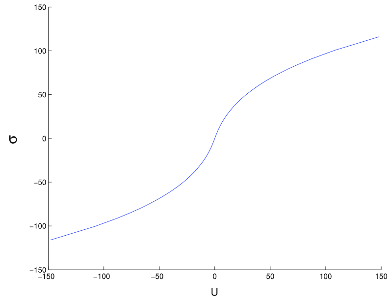
Figure 1: Plot of numerical results for the $\mathcal{O}(t^{0})$ term in the asymptotic expansion of the action versus $U$. The slope at $U=0$ matches the value calculated from (130). The baryon expectation value $\langle\mathcal{A}\rangle\sim\langle\mathcal{B}\rangle^{-1}$ in units of $\Lambda^{2M}_{2M}$ is given by the exponential of this function.

5 Conclusions

In previous work, increasingly convincing evidence has been emerging [10, 13, 14, 15] that the warped deformed conifold background of [10] is dual to the cascading gauge theory with condensates of the baryon operators $\mathcal{A}$ and $\mathcal{B}$. Furthermore, a one-parameter family of more general warped deformed conifold backgrounds was constructed [17, 15] and argued to be dual to the entire baryonic branch of the moduli space, $\mathcal{A}\mathcal{B}=\mathrm{const.}$

In this paper we present additional, and more direct, evidence for this identification by calculating the baryonic condensates on the string theory side of the duality. Following [13, 18], we identify the Euclidean D5-branes wrapped over the deformed conifold, with appropriate gauge fields turned on, with the fields dual to the baryonic operators in the sense of gauge/string dualities. We derive the first order equations for the gauge fields and solve them explicitly. The solutions are subjected to a number of tests. From the behavior of the D5-brane action at large radial cut-off $r$ we deduce the $r$-dependence of the baryon operator dimensions and match it with that in the cascading gauge theory. Furthermore, we use the D5-brane action to calculate the condensates as functions of the modulus $U$ that is explicit in the supergravity backgrounds. We find that the product of the $\mathcal{A}$ and $\mathcal{B}$ condensates indeed does not depend on $U$.

This calculation also establishes a map between the parameterizations of the baryonic branch on the string theory and on the gauge theory sides of the duality. This map should be useful for comparing other physical quantities along the baryonic branch, and we hope to return to such comparisons in the future.

6 Acknowledgements

We thank E. Witten for the initial suggestion that gave the impetus to this project, and S. Gubser for useful discussions. This research was supported in part by the National Science Foundation under Grant No. PHY-0243680. The research of AD is also supported in part by Grant RFBR 04-02-16538, and Grant for Support of Scientific Schools NSh-8004.2006.2. Any opinions, findings, and conclusions or recommendations expressed in this material are those of the authors and do not necessarily reflect the views of the National Science Foundation.

Appendix A Appendix: D5-Brane on the CVMN Background

Here we collect some results for the Euclidean D5-brane in the CVMN background [23, 24]. As emphasized in [15] and above, this background is not part of the baryonic branch since its asymptotic behavior at large $t$ is different from the “cascading behavior” found in [9, 10]. With $h_{2}=\chi=0$ and after substituting the explicit CVMN expressions [17, 23, 24] for the remaining functions, the differential equation (66) simplifies to

$$\xi^{\prime}={-t\sinh(t)\xi\over 2\sqrt{-1+2t\coth(t)-{t^{2}\over\sinh^{2}(t)}}}\left[{\sinh(t)\over 4}\sqrt{-1+2t\coth(t)-{t^{2}\over\sinh^{2}(t)}}-\xi^{2}\right]^{-1}\ .$$ (131)

This is again a total derivative

$${\mathrm{d}\over\mathrm{d}t}\left(-{1\over 3}\,\xi^{3}+{1\over 4}\,\xi\sinh(t)\sqrt{-1+2t\coth(t)-{t^{2}\over\sinh^{2}(t)}}\right)=0\ ,$$ (132)

with three solutions (for zero integration constant), $\xi=0$ and

$$\xi=\pm{\sqrt{3}\over 2}\,\sqrt{\sinh(t)}\,\left(-1+2t\coth(t)-{t^{2}\over\sinh^{2}(t)}\right)^{1/4}=\pm{\sqrt{3}\over 2}\,\sqrt{\sinh(t)}\,e^{g/2}\ ,$$ (133)

where the functional form of $e^{g}$ for the CVMN background can be read off from the last equality. Evaluating the Lagrangian (105) one finds for $\xi=0$

$$e^{-\phi}\sqrt{\mathrm{det}(G+\mathcal{F})}={1\over 8}\,\sinh(t)\,e^{g}\ ,$$ (134)

and for $\xi=\pm\sqrt{3}\,e^{x}$

$$e^{-\phi}\sqrt{\mathrm{det}(G+\mathcal{F})}={1\over 4}\sinh(t)e^{g}\left(1+3t^{2}e^{-2g}\right)\ .$$ (135)

For all three solutions the action clearly diverges exponentially in $t$ as $t\rightarrow\infty$ (this corresponds to a power divergence in $r$). Therefore, the Euclidean D5-brane cannot be interpreted in terms of baryonic condensates. This is in agreement with the fact that the CVMN solution does not belong to the baryonic branch of the cascading gauge theory: its UV asymptotics are completely different from those that define the cascading theories.

Appendix B Appendix: D7-Brane on the Baryonic Branch

In this section we will briefly discuss the case of the D7-brane. The first order equation (62) with $\mathfrak{g}$ given by (63) can be rewritten in a form similar to (66)

$$\xi^{\prime}={e^{g}\over v} \left[{\over}2h_{2}a\sinh^{2}(t)(\xi+\chi)-(1+a\cosh(t))\left((\xi+\chi)^{2}-e^{2x}+h_{2}^{2}\sinh^{2}(t)\right)\right]\times$$ (136)

$$\Big{[}{\over}e^{2g}h_{2}\sinh(t)[1-e^{-2x}((\xi+\chi)^{2}-h_{2}^{2}\sinh(t)^{2})]$$

$$-2\sinh(t)(1+a\cosh(t))[a(\xi+\chi)-h_{2}(1+a\cosh(t))]\,\Big{]}^{-1}\ .$$

Similarly to (92), the $\xi$-dependent part of this equation can be represented as a total derivative

$${d\over dt} \bigg{[} {1\over 3}(\xi+\chi)^{3}+{e^{2x}a\,(1+a\cosh(t))\over h_{2}e^{2g}}(\xi+\chi)^{2}$$

$$- [e^{2x}+h_{2}^{2}\sinh^{2}(t)+2e^{2x}(1+a\cosh(t))^{2}e^{-2g}](\xi+\chi)\bigg{]}$$

$$= - {e^{2x}(1+a\cosh(t))\over vh_{2}\sinh(t)e^{g}}[e^{2x}-h_{2}^{2}\sinh^{2}(t)]$$

$$- [e^{2x}+h_{2}^{2}\sinh^{2}(t)+2e^{2x}(1+a\cosh(t))^{2}e^{-2g}]\chi^{\prime}\ .$$

In analogy to (107) the DBI action for D7 can be represented as the sum of a polynomial in $\xi$ and a $\xi$-independent integral

$$S_{D7}=U\bigg{|} - {1\over 3}\tilde{\xi}^{3}+{ah_{2}\sinh^{2}(t)\over 1+a\cosh(t)}\tilde{\xi}^{2}+\left(e^{2x}-h_{2}^{2}\sinh^{2}(t)\right)\tilde{\xi}$$

$$+ \int_{0}^{t}\bigg{[}{h_{2}\sinh(t)e^{g}\over v(1+a\cosh(t))}[e^{2x}+h_{2}^{2}\sinh^{2}(t)]$$

$$+ {2e^{2x}h_{2}\sinh(t)(1+a\cosh(t))\over ve^{g}}-[e^{2x}-h_{2}^{2}\sinh^{2}(t)]\chi^{\prime}\bigg{]}dt\bigg{|}\ .$$

Interestingly, the coefficients of the characteristic cubic polynomials in (B) and (B) are the same ones we encountered for the D5-brane, except that their roles are switched: $\mathfrak{C},\mathfrak{D}$ and $\sigma$ appear in the differential equation for the gauge field while $\mathfrak{A},\mathfrak{B}$ and $\rho$ appear in the action.

In the KS case (B) simplifies drastically and reduces to (compare with (72))

$$\xi^{3}=3\left({(\sinh(t)\cosh(t)-t)^{2/3}h\over 16}+{(t\coth(t)-1)^{2}\over 4}\right)\xi\ ,$$ (139)

which has the trivial solution $\xi=0$ and a pair of non-zero solutions related to each other by the symmetry $\mathcal{I}$. From the asymptotic expansions (115) of $\mathfrak{A}$ and $\rho$ it is then evident that the action (B) will be exponentially divergent $\sim\mathcal{O}(e^{2t/3})$ for all three solutions.

References

- [1] J. M. Maldacena, “The large N limit of superconformal field theories and supergravity,” Adv. Theor. Math. Phys. 2, 231 (1998) [Int. J. Theor. Phys. 38, 1113 (1999)] [arXiv:hep-th/9711200].
- [2] S. S. Gubser, I. R. Klebanov and A. M. Polyakov, “Gauge theory correlators from non-critical string theory,” Phys. Lett. B 428, 105 (1998) [arXiv:hep-th/9802109].
- [3] E. Witten, “Anti-de Sitter space and holography,” Adv. Theor. Math. Phys. 2, 253 (1998) [arXiv:hep-th/9802150].
- [4] I. R. Klebanov and E. Witten, “Superconformal field theory on threebranes at a Calabi-Yau singularity,” Nucl. Phys. B 536, 199 (1998) [arXiv:hep-th/9807080].
- [5] D. R. Morrison and M. R. Plesser, “Non-spherical horizons. I,” Adv. Theor. Math. Phys. 3, 1 (1999) [arXiv:hep-th/9810201].
- [6] S. S. Gubser and I. R. Klebanov, “Baryons and domain walls in an N = 1 superconformal gauge theory,” Phys. Rev. D 58, 125025 (1998) [arXiv:hep-th/9808075].
- [7] I. R. Klebanov and N. A. Nekrasov, “Gravity duals of fractional branes and logarithmic RG flow,” Nucl. Phys. B 574, 263 (2000) [arXiv:hep-th/9911096].
- [8] N. Seiberg, “Electric - magnetic duality in supersymmetric nonAbelian gauge theories,” Nucl. Phys. B 435, 129 (1995) [arXiv:hep-th/9411149].
- [9] I. R. Klebanov and A. A. Tseytlin, “Gravity duals of supersymmetric SU(N) x SU(N+M) gauge theories,” Nucl. Phys. B 578, 123 (2000) [arXiv:hep-th/0002159].
- [10] I. R. Klebanov and M. J. Strassler, “Supergravity and a confining gauge theory: Duality cascades and chiSB-resolution of naked singularities,” JHEP 0008, 052 (2000) [arXiv:hep-th/0007191].
- [11] C. P. Herzog, I. R. Klebanov and P. Ouyang, “Remarks on the warped deformed conifold,” arXiv:hep-th/0108101; “D-branes on the conifold and N = 1 gauge / gravity dualities,” arXiv:hep-th/0205100.
- [12] M. J. Strassler, “The duality cascade,” arXiv:hep-th/0505153.
- [13] O. Aharony, “A note on the holographic interpretation of string theory backgrounds with varying flux,” JHEP 0103, 012 (2001) [arXiv:hep-th/0101013].
- [14] S. S. Gubser, C. P. Herzog and I. R. Klebanov, “Symmetry breaking and axionic strings in the warped deformed conifold,” JHEP 0409, 036 (2004) [arXiv:hep-th/0405282]; “Variations on the warped deformed conifold,” Comptes Rendus Physique 5, 1031 (2004) [arXiv:hep-th/0409186].
- [15] A. Dymarsky, I. R. Klebanov and N. Seiberg, “On the moduli space of the cascading SU(M+p) x SU(p) gauge theory,” JHEP 0601, 155 (2006) [arXiv:hep-th/0511254].
- [16] N. Seiberg, “Exact Results On The Space Of Vacua Of Four-Dimensional Susy Gauge Theories,” Phys. Rev. D 49, 6857 (1994) [arXiv:hep-th/9402044].
- [17] A. Butti, M. Grana, R. Minasian, M. Petrini and A. Zaffaroni, “The baryonic branch of Klebanov-Strassler solution: A supersymmetric family of SU(3) structure backgrounds,” JHEP 0503, 069 (2005) [arXiv:hep-th/0412187].
- [18] E. Witten, Unpublished, July 2004.
- [19] I. R. Klebanov and E. Witten, “AdS/CFT correspondence and symmetry breaking,” Nucl. Phys. B 556, 89 (1999) [arXiv:hep-th/9905104].
- [20] O. Aharony, A. Buchel and A. Yarom, “Holographic renormalization of cascading gauge theories,” Phys. Rev. D 72, 066003 (2005) [arXiv:hep-th/0506002].
- [21] O. Aharony, A. Buchel and A. Yarom, “Short distance properties of cascading gauge theories,” arXiv:hep-th/0608209.
- [22] G. Papadopoulos and A. A. Tseytlin, “Complex geometry of conifolds and 5-brane wrapped on 2-sphere,” Class. Quant. Grav. 18, 1333 (2001) [arXiv:hep-th/0012034].
- [23] A. H. Chamseddine and M. S. Volkov, “Non-Abelian BPS monopoles in N = 4 gauged supergravity,” Phys. Rev. Lett. 79, 3343 (1997) [arXiv:hep-th/9707176]; A. H. Chamseddine and M. S. Volkov, “Non-Abelian solitons in N = 4 gauged supergravity and leading order string theory,” Phys. Rev. D 57, 6242 (1998) [arXiv:hep-th/9711181].
- [24] J. M. Maldacena and C. Nunez, “Towards the large N limit of pure N = 1 super Yang Mills,” Phys. Rev. Lett. 86, 588 (2001) [arXiv:hep-th/0008001].
- [25] J. Polchinski, “String theory. Vol. 2: Superstring theory and beyond,”
- [26] C. P. Bachas, “Lectures on D-branes,” arXiv:hep-th/9806199.
- [27] C. V. Johnson, “D-brane primer,” arXiv:hep-th/0007170.
- [28] E. Bergshoeff and P. K. Townsend, “Super D-branes,” Nucl. Phys. B 490, 145 (1997) [arXiv:hep-th/9611173].
- [29] E. Bergshoeff and P. K. Townsend, “Super-D branes revisited,” Nucl. Phys. B 531, 226 (1998) [arXiv:hep-th/9804011].
- [30] M. Cederwall, A. von Gussich, B. E. W. Nilsson, P. Sundell and A. Westerberg, “The Dirichlet super-p-branes in ten-dimensional type IIA and IIB supergravity,” Nucl. Phys. B 490, 179 (1997) [arXiv:hep-th/9611159].
- [31] E. Witten, “Baryons and branes in anti de Sitter space,” JHEP 9807, 006 (1998) [arXiv:hep-th/9805112].
- [32] Y. Imamura, “Supersymmetries and BPS configurations on Anti-de Sitter space,” Nucl. Phys. B 537, 184 (1999) [arXiv:hep-th/9807179].
- [33] C. G. Callan, A. Guijosa and K. G. Savvidy, “Baryons and string creation from the fivebrane worldvolume action,” Nucl. Phys. B 547, 127 (1999) [arXiv:hep-th/9810092].
- [34] D. Arean, D. E. Crooks and A. V. Ramallo, “Supersymmetric probes on the conifold,” JHEP 0411, 035 (2004) [arXiv:hep-th/0408210].
- [35] M. Marino, R. Minasian, G. W. Moore and A. Strominger, “Nonlinear instantons from supersymmetric p-branes,” JHEP 0001, 005 (2000) [arXiv:hep-th/9911206].
- [36] L. Martucci and P. Smyth, “Supersymmetric D-branes and calibrations on general N = 1 backgrounds,” JHEP 0511, 048 (2005) [arXiv:hep-th/0507099].
- [37] L. Martucci, “D-branes on general N = 1 backgrounds: Superpotentials and D-terms,” JHEP 0606, 033 (2006) [arXiv:hep-th/0602129].
- [38] A. Iqbal, N. Nekrasov, A. Okounkov and C. Vafa, “Quantum foam and topological strings,” arXiv:hep-th/0312022.
- [39] K. Skenderis, “Lecture notes on holographic renormalization,” Class. Quant. Grav. 19, 5849 (2002) [arXiv:hep-th/0209067].
- [40] A. Karch, A. O’Bannon and K. Skenderis, “Holographic renormalization of probe D-branes in AdS/CFT,” JHEP 0604, 015 (2006) [arXiv:hep-th/0512125].