Quantum broadening of k-strings in gauge theories

Abstract:

We study the thickness of the confining flux tube generated by a pair of sources in higher representations of the gauge group. Using a simple geometric picture we argue that the area of the cross-section of the flux tube, as measured by a Wilson loop probe, grows logarithmically with source separation, as a consequence of the quantum fluctuations of the underlying k-string. The slope of the logarithm turns out to be universal, i.e. it is the same for all the representations and all the gauge theories. We check these predictions in a 3D $\Z_{4}$ lattice gauge model by comparing the broadening of the 1-string and the 2-string.

1 Introduction

In the physics of quark confinement there are many indications that the gauge field responds to a static $q$ source separated from a conjugate $\bar{q}$ source by a large distance $L$ by forming a colour flux tube which behaves as a string with energy $V(L)\simeq\sigma_{\mathscr{R}}\,L$, where the string tension $\sigma_{\mathscr{R}}$ depends on the representation $\mathscr{R}$ of the quantum numbers carried by the source.

If the gauge group is $\mathop{\rm SU}(N)$ there are infinitely many irreducible representations at our disposal to cast the sources. However, for large separations, no matter what representation is chosen, $\sigma_{\mathscr{R}}$ depends only on the $N-$ality $k$ of $\mathscr{R}$, i.e. on the number (modulo $N$) of copies of the fundamental representation needed to build $\mathscr{R}$ by tensor product, the reason being that all representations with the same $k$ can be transformed into each other by the emission of a proper number of soft gluons. As a consequence the heavier strings decay into the string of smallest string tension. The corresponding string is referred to as a k-string.

The spectrum of k-string tensions has been extensively studied in recent years, in the continuum [1]–[8] as well as on the lattice [9]–[16]. In this paper we want to explore another facet of k-string physics, related to the quantum fluctuations of these objects.

It is widespread belief that the flux tube generated by a pair of sources $q$, $\bar{q}$ in the fundamental representation is in the rough phase. This means, as explained long ago by Lüscher, Münster and Weisz [17], that the colour flux tube broadens as the sources are separated. More precisely, the area of a cross-section of the flux tube should increase logarithmically with separation. This phenomenon can be seen as a consequence of the quantum vibrations of the underlying 1-string describing of the infrared properties of this flux tube.

Since the k-strings can be seen as bound states of $k$ 1-strings, it is interesting to ask if there is any fundamental obstruction for a logarithmic broadening of the k-strings. At first sight it is not clear whether in the IR limit the only relevant degrees of freedom are the transverse displacements of a single string or whether we have to take into account new degrees of freedom describing the possible splitting of the $k$-string into its constituent strings. In other terms one would like to know whether the string binding energy damps significantly the quantum fluctuations of the free strings.

The answer we find to the above questions is surprisingly simple: not only the logarithmic broadening occurs in the k-strings for any $k$, but it turns also out that the coefficient of the logarithm does not depend on the specific representation of the source nor on its N-ality and is universal, i.e. it is the same in all gauge theories. We check these predictions in a 3D $\Z_{4}$ gauge model, which is the simplest environment where a non-trivial 2-string can live. A brief report of our work has been presented in [18].

Measuring the thickness of the flux tube and in particular its dependence on the separation of the sources is very challenging from a computational point of view. In $\mathop{\rm SU}(N)$ gauge theories the error bars are too large to draw definite conclusions [19]. As a matter of fact, an uncontroversial observation of logarithmic broadening has been only made in 3D $\Z_{2}$ gauge model, thanks to the efficiency of the Monte Carlo algorithms for its dual, the Ising model [20]. New results on the thickness of the ${\rm SU}(2)$ flux tube near the deconfining point exploiting the integrability of the underlying 2D Ising model appeared recently [21]. The numerical data on the logarithmic growth of the mean squared width of the flux tube associated to the $\Z_{4}$ strings presented here constitute a new important support on the expected quantum behaviour of the flux tube.

2 The rough phase

In the strong coupling phase of whatever gauge theory in three or four space-time dimensions the flux tube joining a quark pair has a constant width for large inter-quark distances. As the coupling constant decreases, the flux tube can undergo a roughening transition. The rough phase is characterised by strong fluctuations of the collective coordinates describing the position of the underlying string and the mean squared width of the flux tube diverges logarithmically when the inter-quark distance goes to infinity [17].

The square width of the flux tube generated by a planar Wilson loop $W_{f}(C)$ in the fundamental representation is defined as the sum of the mean square deviations of the transverse coordinates $h_{j}(\xi_{1},\xi_{2})$ $(j=1,\dots D-2)$ of the underlying string, i.e.

$$w^{2}=\frac{1}{A}\sum_{j=1}^{D-2}\int_{\Omega}\mathrm{d}^{2}\xi\langle(h_{j}(\xi_{1},\xi_{2})-h_{j}^{o})^{2}\rangle\,,$$ (1)

where $\Omega$ is the planar domain bounded by $\partial\,\Omega=C$, $A=\int_{\Omega}\mathrm{d}^{2}\xi$ its area and $h^{o}_{j}$ are the transverse coordinates of the equilibrium position. The vacuum expectation value is taken with respect to the two-dimensional field theory describing the dynamics of the flux tube. It is widely believed that the roughening transition belongs to the Kosterlitz-Thouless universality class [22]. As a consequence, it is expected that this field theory flows, in the infrared (IR) limit, toward the massless free-field theory described by the Gaussian action

$$S_{IR}=\frac{\sigma}{2}\sum_{j=1}^{D-2}\int_{\Omega}\mathrm{d}^{2}\xi\sum_{\mu=1,2}\partial_{\mu}h_{j}\partial^{\mu}h_{j}\,.$$ (2)

In such a limit the mean square width can be easily evaluated in terms of the free Green functions $G_{\Omega}(\xi,\xi^{\prime})=\langle h(\xi)\,h(\xi^{\prime})\rangle$ as

$$w^{2}=\frac{D-2}{A^{2}}\int_{\Omega}\mathrm{d}^{2}\xi\;\int_{\Omega}\mathrm{d}^{2}\xi^{\prime}\left(G_{\Omega}(\xi,\xi^{\prime})-G_{\Omega}(\xi,\xi+\epsilon)\right)\,,$$ (3)

where $\epsilon$ is a UV cut-off. The action (2) is conformally invariant, hence the integration of the finite part $G(\xi,\xi^{\prime})$ cannot depend on the size of the domain $\Omega$ but only on its shape. The logarithmic growth of $w^{2}$ comes from the UV divergent part. This can be simply understood as follows [20]. The conformal invariance of the theory implies the scaling property

$$G_{\Omega}(\xi,\xi^{\prime})=G_{\Omega_{s}}(s\,\xi,s\,\xi^{\prime})\,,$$ (4)

where $s>0$ is an arbitrary real number and $\Omega_{s}$ is the scaled domain. On the other hand in the UV limit $\xi^{\prime}\to\xi$ the Green function diverges logarithmically

$$G_{\Omega}(\xi,\xi+\epsilon)=-\frac{1}{2\pi\sigma}\log\epsilon+\dots\,.$$ (5)

(4) and (5) agree only if the cut-off appears exclusively in the ratio $\epsilon/R$, where $R$ is a typical linear size of the domain. Adding this piece of information to (3) yields

$$w^{2}=\frac{D-2}{2\pi\sigma}\log(R/R_{f}(\Omega))\,,$$ (6)

where the UV cut-off has been absorbed in the scale $R_{f}(\Omega)$, thus the absolute value of this physical scale cannot be determined by this conformal approach. On the contrary the ratios of these scales for different domains are calculable functions of the shapes [20, 23].

It is clear from this approach that the generalisation to the k-string crucially depends on its IR limit. If, for instance, it fluctuated as a single string it would suffice to put $\sigma\to\sigma_{k}$ in (2) and modify the other formulae consequently. There are other possibilities, however. We shall see in the next section that in $D=3$ dimensions there is a geometric approach, first advocated in [17], which can be unambiguously extended to the k-strings.

3 K-strings and minimal surfaces

To inspect the width of the flux tube generated, in a 3D gauge system, by a static source in the fundamental representation one can start, following [17], from the connected correlator

$$P_{f}(h)=\frac{\langle\hskip 1.99997ptW_{f}(C)\,W_{f}(c)\hskip 1.99997pt\rangle-\langle\hskip 1.99997ptW_{f}(C)\hskip 1.99997pt\rangle\langle\hskip 1.99997ptW_{f}(c)\hskip 1.99997pt\rangle}{\langle\hskip 1.99997ptW_{f}(C)\hskip 1.99997pt\rangle}\,,$$ (7)

where $W_{f}(C)$ and $W_{f}(c)$ are Wilson operators for the loops $C$ and $c$, which are concentric circles of radii $R$ and $r<R$ lying on parallel planes at a distance $h$, as shown in Fig. 1. The above quantity can be seen as a measure of the density of the colour flux generated by the source $C$ and felt by the probe $c$.

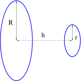
Figure 1: Parallel circular loops

To study the flux generated by sources in a generic representation $\mathscr{R}$, we will take $W_{\mathscr{R}}(C)$ instead of $W_{f}(C)$, but keep the probe always in the fundamental.

The mean square width of the flux tube is defined by

$$w^{2}_{\mathscr{R}}=\frac{\int h^{2}P_{\mathscr{R}}(h)\,\mathrm{d}h}{\int P_{\mathscr{R}}(h)\,\mathrm{d}h}\,.$$ (8)

The insight of [17] was to observe that the quantity $P_{f}(h)$ can be described in the effective string picture in terms of the world-sheet of a Nambu-Goto string connecting the two circles. This defines a typical Plateau problem of minimal surfaces, which can be evaluated in the infrared limit by a saddle-point approximation. More specifically, one can write

$$\langle\hskip 1.99997ptW_{f}(C)\,W_{f}(c)\hskip 1.99997pt\rangle-\langle\hskip 1.99997ptW_{f}(C)\hskip 1.99997pt\rangle\langle\hskip 1.99997ptW_{f}(c)\hskip 1.99997pt\rangle\propto\exp(-\sigma A(R,r,h))\,,$$ (9)

where $A(R,r,h)$ denotes the area of the connected minimal surface having $C$ and $c$ as boundaries.

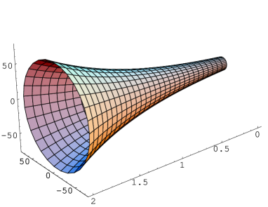
Figure 2: Catenoid surface

The choice of the Nambu-Goto (NG) action for the effective string is the simplest one, however there are well known problems for its quantisation procedure. This theory is fully consistent only at critical space-time dimensions (D=26), but there is strong evidence that the first few terms in the $1/(\sigma\,A)$ expansion of the NG action are universal up to the order $O\left[\frac{1}{(\sigma\,A)^{2}}\right]$ (see [25], and references quoted therein, for a detailed discussion on this point). In particular, the $O(1)$ term coincides with (2), thus it is reasonable to expect that in the infrared limit $R\to\infty$ with fixed $r$ and $h$ the result should not depend on the specific choice of NG action. Note however that the size $r$ of the probe cannot be too small, otherwise the string picture would not be valid.

The minimal surface connecting the two circles is a surface of revolution about the symmetry axis (here chosen to coincide with the $\boldsymbol{x}$ axis). If we denote by $y(x)$ the $y>0$ section of the surface with the $(x,y)$ plane, the area is given by

$$A=2\pi\int_{0}^{h}y\sqrt{\dot{y}^{2}+1}\,\mathrm{d}x\,.$$ (10)

The variational condition $\frac{\delta A}{\delta y(x)}=0$ yields the equation $1+\dot{y}^{2}=y\,\ddot{y}$. The general solution is

$$y(x)=\frac{1}{\omega}\cosh\omega(x-x_{0})\,,$$ (11)

that is, the surface of revolution is a catenoid (see Fig. 2). The integration constants must obey

$$R=\frac{1}{\omega}\cosh\omega x_{0}\quad,\quad r=\frac{1}{\omega}\cosh\omega(h-x_{0})\,.$$ (12)

This results in the following expression for the minimal area:

$$A=\pi\Big{(}\frac{h}{\omega}+R^{2}\sqrt{1-\frac{1}{\omega^{2}R^{2}}}-r^{2}\sqrt{1-\frac{1}{\omega^{2}r^{2}}}\Big{)}\,;$$ (13)

moreover Eq. (12) allows to express $h$ as a decreasing function of $\omega$

$$h(\omega)=\frac{\big{[}{\rm arccosh}(R\omega)-{\rm arccosh}(r\omega)\big{]}}{\omega}\,,$$ (14)

thus we can regard $\omega$ as an integration variable for actually computing $w^{2}$. Using the trivial inequality $\cosh x\geq 1~{}(\forall\,x)$ we get a minimal value for $\omega$, that is a maximal allowed value for $h$:

$$\omega_{min}=\frac{1}{r}\quad\Rightarrow\quad h_{max}=h(1/r)\,.$$ (15)

Now we can write explicitly, for the mean square width,

$$w^{2}=\frac{\int_{\frac{1}{r}}^{\infty}h(\omega)^{2}\,exp[-\sigma A(R,r,h(\omega))]\,|h^{\prime}(\omega)|\,d\omega}{\int_{\frac{1}{r}}^{\infty}\,exp[-\sigma A(R,r,h(\omega))]\,|h^{\prime}(\omega)|\,d\omega}\,.$$ (16)

This quantity approaches a logarithmic curve for large $R$. Indeed, this can be seen by using the asymptotic expansion

$${\rm arccosh}(\omega r)\sim 2\log(\omega r)\;\;\;\;(\omega r\to\infty)\,,$$ (17)

and inserting it into (14), which yields the approximate solution found in [17]:

$$\omega\sim\frac{1}{h}\log(R/r)\,.$$ (18)

The condition $\omega r\gg 1$ becomes

$$\log(R/r)\gg h/r\,,$$ (19)

always fulfilled in the large $R$ limit. Note that $r$ cannot be too small at fixed $R$ and $h$. In this limit, a Gaussian distribution is found for the transversal density, whose width grows logarithmically with $R$:

$$P^{(R)}(h)\propto\exp\left[-\frac{\sigma\pi h^{2}}{\log(R/r)}\right]\quad\Rightarrow\quad\sigma w^{2}=\frac{1}{2\pi}\log(R/r)\,,$$ (20)

which is almost identical to (6). Here the UV cut-off is replaced by the size $r$ of the probe.

The result found here can be generalised to Wilson loop $W_{\mathscr{R}}(C)$ in any representation (where we are no more guaranteed that the infrared Gaussian free string limit is valid). The world-sheet of the k-string can be seen as some bound state of $k$ 1-string world-sheets. In this case a local minimum solution exists for sure, in which one of these fundamental sheets gives rise to the catenoid with the probe $W_{f}(c)$, while the other $k-1$ just lie flat on the loop surface. We then have immediately

$$P^{(R)}_{(k)}(h)=P^{(R)}_{(1)}(h)\cdot\exp[\pi R^{2}(\sigma_{k}-\sigma_{k-1}-\sigma)]\,,$$ (21)

where the stability of the k-string implies that the exponent is always negative. The resulting width, then, appears to be exactly the same as for the fundamental representation.

3.1 Special configurations

In some special cases, for a very narrow range of $h$, there is, beside the above general solution, another minimal surface made by a first catenoid composed by the k-string world-sheet.

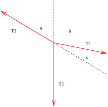
Figure 3: The balance of the string tensions

At a suitable distance $d$ it splits into a disk orthogonal to the symmetry axis made by the world-sheet of the $(k-1)$-string and a second catenoid in the fundamental representation which reaches the probe $c$. The position of the intermediate disk is not arbitrary, but it is dynamically determined by the balance of the tensions at the string junction. In the most general configuration depicted in Fig. 3 a $k_{2}$-string propagating along a catenoid decays into a $k_{3}$-string forming a disk and a $k_{1}$-string forming another catenoid. The angles of the string junction are given by

$$\cos\theta_{1}=\frac{\sigma_{k_{2}}^{2}+\sigma_{k_{3}}^{2}-\sigma_{k_{1}}^{2}}{2\sigma_{k_{2}}\sigma_{k_{3}}}\,,$$ (22)

and cyclic permutations of the indices for the other angles.

Implementing these kinematic constraints on the parameters $\omega_{0},x_{0}$ and $\omega_{1},x_{1}$ of the two catenoids yields

$$\omega_{0}\,R= \cosh\omega_{0}\,x_{0}~{},\,\omega_{0}\,\rho=\cosh\omega_{0}(x_{0}-d)=1/\sin\theta_{1}\,,$$ (23)

$$\omega_{1}\,r= \cosh\omega_{1}(x_{1}+d-h)~{},\,\omega_{1}\,\rho=\cosh\omega_{1}x_{1}=1/\sin\theta_{2}\,,$$ (24)

where $d$ is the distance of the disk from the source and $\rho$ its radius. We can invert these relations and express $d$ and $h$ as functions of $\rho$

$$d(\rho)= \rho\,\sin\theta_{1}\,{\rm arccosh}(R/\rho\,\sin\theta_{1})-\rho\,\sin\theta_{1}\,{\rm arccosh}(1/\sin\theta_{1})~{},$$ (25)

$$h(\rho)= \rho\,\sin\theta_{2}\,{\rm arccosh}(1/\sin\theta_{2})-\rho\,\sin\theta_{2}\,{\rm arccosh}(r/\rho\,\sin\theta_{2})+d(\rho)\,.$$ (26)

Both $d(\rho)$ and $h(\rho)$ turn out to be increasing functions of $\rho$. Since $h\geq d$ we have $\rho\geq r$ which implies $\theta_{2}\geq\frac{\pi}{2}$, as Fig. 3 shows, then (22) tells us that this special surface is permitted only if the kinematic constraint

$$\sigma_{k_{2}}^{2}\geq\sigma^{2}_{k_{1}}+\sigma^{2}_{k_{3}}$$ (27)

holds, i.e. only when the binding energy of the $k$-string is sufficiently small. On the other hand, the fact that the argument of ${\rm arccosh}$ must be larger or equal to 1 fixes the maximum $\rho_{max}=r/\sin\theta_{2}$. Thus the minimal surface exists only in the range

$$h(r)\leq h(\rho)\leq h(r/\sin\theta_{2})\,,$$ (28)

which turns out to be in general very narrow. These special configurations should produce a spike in the distribution of the flux density at the distance fixed by (28).

The hight of such a peak is determined by the total area of the surface. Unfortunately this area depends significantly on $r$, hence it is rather unclear how to extract physical information on the flux tube, which should not depend on the size of the probe.

In the $N=4$, $k=2$ case, which corresponds to our simulations, this special solution should obey the constraint (27) i.e. $\sigma_{2}\geq\sqrt{2}\,\sigma$. In our numerical data taken in that region we did not find signs of such a singular behaviour.

4 $\Z_{4}$ gauge theory and its dual

The laboratory where we study the physical properties of the 2-string is a $\Z_{4}$ gauge model in three dimensions, defined by the standard plaquette action on a cubic lattice. With $\Z_{4}$ as gauge group, there exist two k-strings in the system: the fundamental string and the 2-string (related to the double-fundamental representation $f\otimes f$). Moreover, since there are no more representations than one in the same N-ality class, the system does not exhibit any meta-stable string that could spoil the results at finite $R$.

It is well known that this model, as any three-dimensional abelian gauge model, admits a spin model as its dual (see for instance [26]) and any physical property of the gauge system can be translated into a corresponding property of its spin dual. From a computational point of view it is of course much more convenient to work directly on the spin model where powerful non-local cluster algorithms can be applied.

In our case the dual is a spin model with global $\Z_{4}$ symmetry which can be written as a symmetric Ashkin-Teller (AT) model [27], i. e. two coupled, ferromagnetic, Ising models defined by the two-parameter action

$$S_{AT}=-\sum_{\langle xy\rangle}\Big{[}\beta(\sigma_{x}\sigma_{y}+\tau_{x}\tau_{y})+\alpha(\sigma_{x}\sigma_{y}\tau_{x}\tau_{y})\Big{]}\,,$$ (29)

where $\sigma_{x}$ and $\tau_{x}$ are the Ising variables ($\sigma,\tau=\pm 1$) associated to the site $x$ and the sum is over all the links $\langle xy\rangle$ of the dual cubic lattice. The phase diagram of this model has been studied long ago [28, 29].

The global $\Z_{4}$ symmetry of the action is generated by the transformation

$$\sigma\to-\tau\>;\>\tau\to\sigma\,.$$ (30)

The model has also an independent $\Z_{2}$ symmetry generated by

$$\sigma\leftrightarrow\tau\,,$$ (31)

related to the charge conjugation of the corresponding dual model.

It is customary to represent the $\Z_{4}$ symmetry through the multiplication table of the fourth roots of the identity ($\xi_{j}=\pm i,\pm 1$). It would be a simple exercise to rewrite the AT model with this kind of variables introducing the complex field

$$\Psi_{x}=e^{-i\frac{\pi}{4}}(\sigma_{x}+i\tau_{x})\,,$$ (32)

where the phase factor is chosen such that the $\Z_{2}$ symmetry defined above becomes the complex conjugation $\Psi\leftrightarrow\Psi^{\star}$. The $\Z_{4}$ symmetry, instead, corresponds to the multiplication by $i$.

The standard application of the duality transformation would lead to a gauge model on the dual lattice with a $\{\xi_{j}\}$-valued field on the links and with an action containing plaquette operators and their squares:

$$S=-\sum_{p}\left[c_{1}\mathfrak{Re}(U_{p})+c_{2}(U_{p})^{2}\right]\,.$$ (33)

We think it is interesting (and more purposeful for our work) to show that the AT model is dually equivalent to two coupled $\Z_{2}$ gauge models.

The starting point is to rewrite the Boltzmann factors associated to the links in the known form, namely the $\Z_{2}$ character expansion

$$e^{\beta\,\sigma_{x}\sigma_{y}} = \sqrt{\frac{\sinh 2\beta}{2}}\sum_{\mu_{\langle xy\rangle}=\pm 1}e^{\stackrel{{\scriptstyle\sim}}{{\beta}}\,\mu_{\langle xy\rangle}}(\sigma_{x}\sigma_{y})^{\hat{\mu}_{\langle xy\rangle}}$$ (34)

$$e^{\beta\,\tau_{x}\tau_{y}} = \sqrt{\frac{\sinh 2\beta}{2}}\sum_{\nu_{\langle xy\rangle}=\pm 1}e^{\stackrel{{\scriptstyle\sim}}{{\beta}}\,\nu_{\langle xy\rangle}}(\tau_{x}\tau_{y})^{\hat{\nu}_{\langle xy\rangle}}$$ (35)

$$e^{\alpha\,\sigma_{x}\sigma_{y}\tau_{x}\tau_{y}} = \sqrt{\frac{\sinh 2\alpha}{2}}\sum_{\rho_{\langle xy\rangle}=\pm 1}e^{\stackrel{{\scriptstyle\sim}}{{\alpha}}\,\rho_{\langle xy\rangle}}(\sigma_{x}\sigma_{y}\tau_{x}\tau_{y})^{\hat{\rho}_{\langle xy\rangle}}$$ (36)

with $\stackrel{{\scriptstyle\sim}}{{\gamma}}=-\log\sqrt{\tanh\gamma}$ and $\hat{\eta}=\frac{1}{2}-\frac{\eta}{2}$.

Now the sum over the site variables $\sigma$ and $\tau$ can be explicitly performed, yielding for each node $x$ the two conservation laws

$$\sum_{y}\left(\hat{\mu}_{\langle xy\rangle}+\hat{\rho}_{\langle xy\rangle}\right)\equiv 0\>\textrm{mod }2\>\textrm{,}\>\sum_{y}\left(\hat{\nu}_{\langle xy\rangle}+\hat{\rho}_{\langle xy\rangle}\right)\equiv 0\>\textrm{mod }2$$ (37)

or, equivalently, in the multiplicative form

$$\prod_{y}\mu_{\langle yx\rangle}\rho_{\langle yx\rangle}=1~{}~{}~{}\>\textrm{,}\>\prod_{y}\nu_{\langle yx\rangle}\rho_{\langle yx\rangle}=1\,.$$ (38)

The canonical partition function becomes

$$Z_{AT}\propto\sum^{{}^{\prime}}_{\mu=\pm 1,\nu=\pm 1,\rho=\pm 1}\exp{\sum_{\langle xy\rangle}\left[\stackrel{{\scriptstyle\sim}}{{\beta}}(\mu_{\langle xy\rangle}+\nu_{\langle xy\rangle})+\stackrel{{\scriptstyle\sim}}{{\alpha}}\rho_{\langle xy\rangle}\right]}\,.$$ (39)

The apex in the sum over configurations indicates that they must obey the constraints (38). A way to solve them in an infinite lattice is suggested by the usual duality transformation of the three-dimensional Ising model: it is sufficient to consider the two composed link variables $\mu_{\langle yx\rangle}\rho_{\langle xy\rangle}$ and $\nu_{\langle xy\rangle}\rho_{\langle xy\rangle}$ as the plaquette variables of the dual lattice. More precisely we solve the above constraints with the Ansatz

$$\mu_{\langle xy\rangle}=\epsilon_{\langle xy\rangle}U_{P}\>,\>\nu_{\langle xy\rangle}=\epsilon_{\langle xy\rangle}V_{P}\>,\>\rho_{\langle xy\rangle}=\epsilon_{\langle xy\rangle}U_{P}V_{P}\>,$$ (40)

here $\epsilon$ is an arbitrary sign variable ($\epsilon=\pm 1$), $P$ is the plaquette dual to the link $\langle xy\rangle$. The plaquette variables are defined through the product of their boundary links, namely,

$$U_{P}=\sum_{\ell\in\partial P}U_{\ell}\>,\>V_{P}=\sum_{\ell\in\partial P}V_{\ell}\>,$$ (41)

where $\ell$ are links of the dual lattice, of course. It is a straightforward exercise to verify that the above Ansatz solves identically Eq.s (38). The sum over the $\epsilon$ variables is unconstrained and can be performed at once, leading to

$$Z_{AT}\propto\sum_{\{U_{\ell}=\pm 1,V_{\ell}=\pm 1\}}\prod_{P}\cosh\big{[}\stackrel{{\scriptstyle\sim}}{{\beta}}(U_{P}+V_{P})+\stackrel{{\scriptstyle\sim}}{{\alpha}}U_{P}V_{P}\big{]}\>.$$ (42)

As the last step, we can rewrite this partition function in the usual Boltzmann form by defining

$$c\,e^{b(U_{P}+V_{P})+aU_{P}V_{P}}=\cosh\big{[}\stackrel{{\scriptstyle\sim}}{{\beta}}(U_{P}+V_{P})+\stackrel{{\scriptstyle\sim}}{{\alpha}}U_{P}V_{P}\big{]}\>.$$ (43)

where $a$, $b$, $c$ are suitable coefficients. Solving for $a$, $b$, $c$ we get

$$c^{4} = \cosh(2\stackrel{{\scriptstyle\sim}}{{\beta}}+\stackrel{{\scriptstyle\sim}}{{\alpha}})\cosh(2\stackrel{{\scriptstyle\sim}}{{\beta}}-\stackrel{{\scriptstyle\sim}}{{\alpha}})\cosh^{2}\stackrel{{\scriptstyle\sim}}{{\alpha}}$$ (44)

$$e^{4b} = \frac{\cosh(2\stackrel{{\scriptstyle\sim}}{{\beta}}+\stackrel{{\scriptstyle\sim}}{{\alpha}})}{\cosh(\stackrel{{\scriptstyle\sim}}{{\beta}}-\stackrel{{\scriptstyle\sim}}{{\alpha}})}$$ (45)

$$e^{4a} = \frac{\cosh(2\stackrel{{\scriptstyle\sim}}{{\beta}}+\stackrel{{\scriptstyle\sim}}{{\alpha}})\cosh(2\stackrel{{\scriptstyle\sim}}{{\beta}}-\stackrel{{\scriptstyle\sim}}{{\alpha}})}{\cosh^{2}\stackrel{{\scriptstyle\sim}}{{\alpha}}}$$ (46)

therefore we can recast $Z_{AT}$ as the partition function of two coupled $\Z_{2}$ gauge systems

$$Z_{AT}(\beta,\alpha)\propto\sum_{\{U_{\ell}=\pm 1,V_{\ell}=\pm 1\}}\prod_{P}e^{b\,(U_{P}+V_{P})+a\,U_{P}V_{P}}\,,$$ (47)

where the duality transformation $\mathscr{D}:(\alpha,\beta)\to(a,b)$ from the AT couplings to the gauge couplings can be explicitly written, using (45) and (46), as

$$a = \frac{1}{4}\ln\Big{(}\frac{(\coth\beta+\tanh\beta\tanh\alpha)(\coth\beta+\tanh\beta\coth\alpha)}{2+\tanh\alpha+\coth\alpha}\Big{)}$$ (48)

$$b = \frac{1}{4}\ln\Big{(}\frac{1+\tanh^{2}\beta\tanh\alpha}{\tanh^{2}\beta+\tanh\alpha}\Big{)}\,\,.$$ (49)

As a non-trivial check of these formulae one can verify that the $\mathscr{D}$ transformation is an involutory automorphism, i. e. $\mathscr{D}^{2}=1$, as required for any duality transformation.

4.1 Dual of a Wilson loop

The duality transformation maps any physical observable of the gauge theory into a corresponding observable of the spin model. In particular it is well known that the Wilson loops are related to suitable twists of the couplings of the spin model. More specifically, let us consider a $\Z_{N}$ spin model in 3D. Let $\xi=e^{i2\pi/N}$ be the generator of this group. A $k$-twist of the link $\langle xy\rangle$ in the spin action is defined by the substitution $\beta\to\xi^{k}\beta$ only in the selected link. Denoting with $Z_{\langle xy\rangle,k}$ the spin partition function modified in this way, one can easily prove the identity

$$\langle\hskip 1.99997ptU_{P}^{(k)}\hskip 1.99997pt\rangle_{gauge}=Z_{\langle xy\rangle,k}/Z\,,$$ (50)

where $P$ is the plaquette dual to $\langle xy\rangle$ and $U_{P}^{(k)}$ is the plaquette variable in the irreducible representation of $\Z_{N}$ characterised by the integer $k=1,2,\ldots,N$. A simple check is the following. The twist of the spin variable associated to a single node is equivalent to twisting all the links incident to this node; on the other hand the twist of a single spin can be re-absorbed in the invariance of the measure of the partition function. On the gauge side, this corresponds to the fact that the product of the plaquette variables lying on the six faces of the cube dual to the selected node is identically equal to 1.

Repeating the above construction for a suitable set of plaquettes we can construct in this way any Wilson loop or Polyakov-Polyakov correlator in any representation and its map into the spin model.

We want to fit this procedure to the AT model. In this case twisting a link corresponds to associating to it an anti-ferromagnetic coupling, i. e.  $\beta\to-\beta$. The character expansion (34) for an anti-ferromagnetic Boltzmann factor becomes simply

$$e^{-\beta\,\sigma_{x}\sigma_{y}}=\sqrt{\frac{\sinh 2\beta}{2}}\sum_{\mu_{\langle xy\rangle}=\pm 1}\mu_{\langle xy\rangle}\;e^{\stackrel{{\scriptstyle\sim}}{{\beta}}\,\mu_{\langle xy\rangle}}\;(\sigma_{x}\sigma_{y})^{\,\hat{\mu}_{\langle xy\rangle}}\,\,.$$ (51)

Notice that in the AT model there are three different couplings associated to a single link. Which of them do we have to twist in order to build on the gauge side the plaquette in the fundamental (i. e. $k=1$) representation? To answer this question it suffices to twist, for instance, the variable $\sigma_{x}\to-\sigma_{x}$. From the point of view of the symmetries of the AT model, such a twist corresponds to a $\Z_{4}$ generator (30) followed by a charge conjugation (31); this corresponds to $\Psi_{x}\to-i\,\Psi_{x}^{*}$ in terms of the complex variable defined in (32), hence it is associated to the fundamental representation. On the other hand this change of sign yields the twist of two couplings for each link incident to $x$: the quadratic $\sigma$ coupling and the quartic coupling. Therefore the plaquette in the fundamental representation is simply obtained by multiplying the Boltzmann factor by $\mu_{\langle xy\rangle}\,\rho_{\langle xy\rangle}=V_{P}$, where we used (40). In this way, the identity outlined above can be written explicitly as

$$\langle\hskip 1.99997ptV_{P}\hskip 1.99997pt\rangle_{gauge}=\langle\hskip 1.99997pte^{-2(\beta+\alpha\tau_{x}\tau_{y})\sigma_{x}\sigma_{y}}\hskip 1.99997pt\rangle_{AT}$$ (52)

generalising the known dual identity of the Ising model. Similarly, flipping the signs of both spins $\sigma_{x}$ and $\tau_{x}$ we get the plaquette variable in the $k=2$ representation as $\langle\hskip 1.99997ptU_{P}V_{P}\hskip 1.99997pt\rangle$. Combining together a suitable set of plaquettes we may build up any Wilson loop or Polyakov-Polyakov correlator with $k=1$ or $k=2$.

The reason why we insist in writing this model in terms of Ising variables is that here one can easily apply a very efficient non-local cluster method [31] which generalises in a straightforward way the one commonly used in Ising systems, based on the Fortuin-Kasteleyn (FK) cluster representation. Moreover, it has been built a very powerful method to estimate Wilson loops $\langle\hskip 1.99997ptW_{\gamma}\hskip 1.99997pt\rangle$ based on the linking properties of the FK clusters [32]: for each FK configuration generated by the above-mentioned algorithm one looks for paths in the cluster linked with the loop $\gamma$. If there is no path of this kind we put $W_{\gamma}=1$, otherwise we set $W_{\gamma}=0$. This method leads to an estimate of $\langle\hskip 1.99997ptW_{\gamma}\hskip 1.99997pt\rangle$ with reduced variance with respect to the conventional numerical estimates.

5 Monte Carlo simulations

We performed a Monte Carlo analysis on the AT model, for both the fundamental and the double-fundamental strings, at the (confining) coupling $(\alpha,\beta)=(0.0070,0.1975)$ (for which we have measured the string tensions $a^{2}\sigma=0.01560(1)$ and $a^{2}\sigma_{2}=0.0210(6)$ [30]).

On the lattice, the quantity $P_{\mathscr{R}}(h)$ is measured by placing a square $R\times R$ loop $W(R)$ on a plane in the desired representation and taking the probe as a plaquette operator, parallel to the loop and lying on its axis at a distance $h$. The actual single measurement took into average also the four planar neighbours of the plaquette in the central position, in order to enhance the signal; this operation does not spoil the results since we dealt with large values of $R$.

According to the recipe for embedding the presence of a Wilson loop (in the representation $\mathscr{R}$) directly into the action as a series of frustrated links, the algorithm has only to measure the expectation value $\langle\hskip 1.99997ptU_{p}^{f}\hskip 1.99997pt\rangle^{W_{\mathscr{R}}}$ of the probe plaquette in the fundamental representation, where the superscript outside the average symbol denotes the fact that the action is modified to include the loop $W(C)$ according to (7)

$$P_{\mathscr{R}}(h)\propto\langle\hskip 1.99997ptU_{P}^{f}\hskip 1.99997pt\rangle^{W_{\mathscr{R}}}+\mathrm{constant}\,.$$ (53)

In terms of AT variables, measuring a plaquette operator translates to measuring the coupling energy on its dual link $\langle xy\rangle$ (the sign variable $\epsilon$ is equal to $+1$ for every link except those dual to the loop, where its value reflects the applied frustration)

$$\langle\hskip 1.99997ptU_{P}^{f}\hskip 1.99997pt\rangle^{W_{\mathscr{R}}}_{gauge}\stackrel{{\scriptstyle\sim}}{{\propto}}\langle\hskip 1.99997pt\epsilon\sigma_{x}\sigma_{y}\hskip 1.99997pt\rangle_{AT}+\mathrm{constant}\,.$$ (54)

The algorithm used for the analysis uses a cluster update method [31] basically similar to the standard Fortuin-Kasteleyn cluster technique: each update step is composed by an update of the $\sigma$ variables using the current values of the $\tau$ as a background (thus locally changing the coupling from $\beta$ to $\beta\pm\alpha$ according to the value of $\tau_{x}\tau_{y}$ on the link $\langle xy\rangle$), followed by an update of the $\tau$’s using the $\sigma$ values as background.

Note that since the large loop is automatically handled by the update procedure and the probe is a loop of side $1$ there is no need to implement expensive topological analysis on the configuration to get the measures, allowing us to reach a performance, with the lattices we used, of about 0.35 seconds per update/measurement step (as on a single Intel ® Xeon 3.2 GHz 64-bit processor). We used a cubic $L^{3}$ lattice with side $L=80$ (we found there are no finite size deviations up to $R\simeq L/2$) and measured $N$ times the plaquette operator as discussed. Configuration results have been then packed in groups of 25 in a binning fashion to estimate variances. We performed the measurements on loop sides $R=11,13,\ldots,41$ with a statistics of 220875 measures (with independent configurations for each $R$) for the fundamental representation and 470275 for the $k=2$ case.

6 Results

The argument based on the properties of the minimal surfaces describing the world-sheet of the underlying confining string suggests a logarithmic growth of the mean square width of the flux tube for both the fundamental and the double-fundamental ($k=2$) string. Also the numerical values of the two functions $w^{2}_{k}(R)$ at fixed $R$ should coincide, but this prediction is easily spoiled by artifacts of the short-range difference between a bound state of two strings and a fundamental string.

\psfrag{Transversal P(h) for k=2 and R=23}{$~{}$}\psfrag{<link>}{$\langle\hskip 1.99997pt\epsilon\sigma_{x}\sigma_{y}\hskip 1.99997pt\rangle_{AT}$}\includegraphics[width=284.52756pt,angle={270}]{transversal_ff_R23.eps}

Figure 4: Typical ($k=2$, $R=23$) transversal flux density distribution, as measured with the quantity in Eq. (54). Note the mismatch with the Gaussian form and the bad background estimate that would follow from the Gaussian assumption for $P(h)$

\psfrag{R sqr(sigma)}{$R\sqrt{\sigma}$}\psfrag{w^2 sigma}{$w^{2}\sigma$}\psfrag{w2_FF}{w2 FF}\psfrag{w2_F}{w2 F}\psfrag{Flux tube width, F vs. FF}{$~{}$}\includegraphics[width=284.52756pt,angle={270}]{w2s_newfit_zmax12.eps}

Figure 5: Flux tube width, $k=1$ versus $k=2$

We found that the measured values of $P_{\mathscr{R}}(h)$ do not fit too well to a normal distribution as approximately expected and lead to bad width estimates (see Fig. 4), so we used the numerically integrated quantities instead, as in eq. (8). We performed the integration by carefully choosing a cutoff value $h_{max}$: since the background value must be subtracted from the transverse flux density functions, the results are very sensitive to the choice of a cutoff. We took $h_{max}=12$. To estimate this background value, we looked for a plateau in the region $|h|\geq h_{min}^{bg}$, separately for each $R$, and took as final value the broadest averaged result in the range $h_{min}^{bg}=18,\ldots,24$.

By fitting the functions $w^{2}_{k=1,2}(R)$, for $R\geq R_{min}$ with $R_{min}$ an appropriate distance cutting off non-IR contributions, to the functional form

$$\sigma\,w^{2}(R)=\frac{1}{2\pi}\log R+c$$ (55)

(see Fig.5) we found that the fundamental string width, as well as the 2-string, show the expected logarithmic growth with the appropriate universal multiplicative factor (reduced $\chi^{2}$ were, respectively, 1.22 and 2.68), but the value of $c$ differs measurably in the two cases: $c_{1}=0.4002(20)$, $c_{2}=0.4512(11)$; this discrepancy is probably due to some interaction between the fundamental world-sheets in the $k=2$ case.

Our work reinforces the numerical evidences of the predicted logarithmic broadening of the flux tube width [20], extending them with high precision to the case of $\Z_{4}$, the simplest gauge group with more than one kind of k-string. In particular, the main result is that, when dealing with a non-fundamental string, its effective width still grows with the logarithmic law. This suggests that here the assumption of a free massless string behaviour for large $R$ holds from the $k=1$ case.

7 Conclusions

In the context of $\mathop{\rm SU}(N)$ gauge theories we have studied the thickness of the confining flux tube generated by a pair of static sources in higher representations as probed by a Wilson loop in the fundamental representation, whose extension is small compared with the source separation. Generalising a simple confining string picture proposed long time ago by Lüscher Münster and Weisz [17] we argued that mean square width $w^{2}$, when measured in terms of fundamental string tension units $\sigma$, grows logarithmically with the source separation $R$ in a manner which is universal, i.e.

$$\sigma\,w^{2}=\frac{D-2}{2\pi}\log\,R/R_{c}\,.$$ (56)

The reference scale $R_{c}$ cannot be directly determined by the underlying string model and it is the only place where one can envisage a dependence on the source representation.

We performed a careful verification of these predictions in the case of a 3D $\Z_{4}$ gauge theory, which is the simplest gauge system where a 2-string forms.

To reach the required high precision of the numerical data, the simulations where actually performed in the dual version of the system, which turns out to be a symmetric Ashkin-Teller model [27]. This choice allowed us to use efficient non-local cluster algorithms [31]. The results of this analysis compare very favourably with the above predictions.

References

- [1] M.R. Douglas and S.H. Shenker, Nucl. Phys. B 447 (1995) 271 [hep-th/9503163].
- [2] A. Hanany, M.J. Strassler and A. Zaffaroni, Nucl. Phys. B 513 (1998) 87 [hep-th/9707244].
- [3] C.P. Herzog and I. R. Klebanov, Phys. Lett. B 526 (2002) 388 [hep-th/0111078].
- [4] A. Armoni and M. Shifman, Nucl. Phys. B 671 (2003) 67 [hep-th/0307020].
- [5] F. Gliozzi, J. High Energy Phys. 08 (2005) 063 [hep-th/0507016].
- [6] F. Gliozzi, Phys. Rev. D 72 (2005) 055011 [hep-th/0504105].
- [7] Y. Imamura, Prog. Theor. Phys. 115 (2006) 815 [hep-th/0512314].
- [8] A. Armoni and B. Lucini, J. High Energy Phys. 0606 (2006) 036 [hep-th/0604055].
- [9] B. Lucini and M. Teper, Phys. Lett. B 501 (2001) 128 [hep-lat/0012025].
- [10] B. Lucini and M. Teper, J. High Energy Phys. 06 (2001) 050 [hep-lat/0103027].
- [11] B. Lucini and M. Teper, Phys. Rev. D 64 (2001) 105019 [hep-lat/0107007].
- [12] B. Lucini, M. Teper and U. Wegler, J. High Energy Phys. 04 (2004) 012 [hep-lat/0404008].
- [13] Y. Koma, E. M. Ilgenfritz, H. Toki and T. Suzuki, Phys. Rev. D 64 (2001) 011501 [hep-ph/0103162].
- [14] L. Del Debbio, H. Panagopoulos, P. Rossi and E. Vicari, Phys. Rev. D 65 (2002) 021501 [hep-th/0106185].
- [15] L. Del Debbio, H. Panagopoulos, P. Rossi and E. Vicari, J. High Energy Phys. 01 (2002) 009 [hep-th/0111090].
- [16] L. Del Debbio, H. Panagopoulos and E. Vicari, J. High Energy Phys. 0309 (2003) 034 [hep-lat/0308012].
- [17] M. Lüscher, G. Münster and P. Weisz, Nucl. Phys. B 180 (1981) 1.
- [18] P. Giudice, F. Gliozzi and S. Lottini, PoS(LAT2006) 70 [hep-lat/0609060].
- [19] G. S. Bali, C. Schlichter and K. Schilling, Phys. Rev. D 51 (1995) 5165.
- [20] M. Caselle, F. Gliozzi, U. Magnea and S. Vinti, Nucl. Phys. B 460 (1996) 397 [hep-lat/9510019].
- [21] M. Caselle, P. Grinza and N. Magnoli, J. Stat. Mech. 0611 (2006) P003 [hep-th/0607014].
- [22] J.M. Kosterlitz and D.J. Thouless, J. Phys. C 6 (1973) 1181.
- [23] K. Pinn, [cond-mat/9909206].
- [24] J. Polchinski and A. Strominger, Phys. Rev. Lett. 67 (1991) 1681.
- [25] J. Kuti, Proceedings of Lattice 2005, PoS(LAT2005) 001 [hep-lat/0511023].
- [26] C. Itzykson and J.-M. Drouffe, Statistical field Theory, Cambridge University Press, 1989.
- [27] J. Ashkin and E. Teller, Phys. Rev. 64 (1943) 178.
- [28] R. V. Ditzian, J. R. Banavar, G. S. Grest and L. P. Kadanoff, Phys. Rev. 22 (1980) 2542.
- [29] P. Arnold and Y. Zhang, Nucl. Phys. B 501 (1997) 803 [hep-lat/9610032].
- [30] P. Giudice, F. Gliozzi and S. Lottini, PoS(LAT2006) 65 [hep-lat/0609055].
- [31] S. Wiseman and E. Domany, Phys. Rev. E 48 (1993) 4080 [hep-lat/9310015].
- [32] F.Gliozzi and S. Vinti, Nucl. Phys. 53 (Proc. Suppl.) (1997) 593 [hep-lat/9609026].