String Cosmology

1 Dark Energy

1.1 The problem of scales

In preparing a set of lectures on string cosmology, I originally set out to explain why I am going to focus exclusively on inflation from string theory, ignoring the important question of the dark energy of the universe, which is another very exciting area on the observational side. The basic reason is that the string scale is so much greater than the scale of the dark energy that it seems implausible that a stringy description should be needed for any physics that is occuring at the milli-eV scale.

Naively, one can generate small energy scales from string-motivated potentials; for example exponential potentials often arise, so that one might claim a quintessence-like Lagrangian of the form

$${\cal L}=(\partial\phi)^{2}-\Lambda e^{-\alpha\phi}$$ (1.1)

could be derived from string theory, and the small scale of the current vacuum energy could be a result of $\phi$ having rolled to large values. The problem with this kind of argument is that it is ruled out by 5th force constraints, unless $\phi$ happens to be extremely weakly coupled to matter. But in string theory, there is no reason for any field to couple with a strength that is suppressed compared to the gravitational coupling, so it seems difficult to get around this problem. The Eöt-Wash experiment [1] bounds the strength of this particle’s coupling to matter as a function of its inverse mass (the range of the 5th force which it mediates) as sketched in figure 1. The current limit restricts a fifth force of gravitational strength to have a range less than $0.044$ mm, corresponding to a mass greater than $4.4$ milli-eV. On the other hand a field that is still rolling today must have a mass less than the current Hubble parameter, $\sim 10^{-33}$ eV.

Fig. 1. Schematic limit on coupling strength versus range of a fifth force.

1.2 The string theory landscape

On the other hand, if we accept the simplest hypothesis, which is also in good agreement with the current data, that the dark energy is just a cosmological constant $\Lambda$, then string theory does have something to tell us. The vast landscape of string vacua [2], combined with the selection effect that we must be able to exist in a given vacuum in order to observe it (the anthropic principle) has given the only plausible explanation of the smallness of $\Lambda$ to date.

We can illustrate the idea starting with a toy model, of a scalar field with Lagrangian

$${\cal L}=(\partial\phi)^{2}-V(\phi)$$ (1.2)

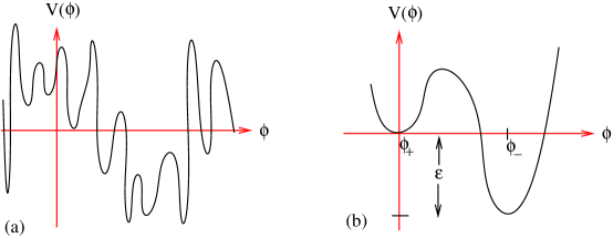
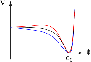
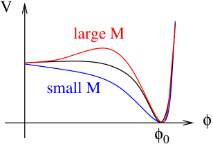
whose potential has many minima, as shown in figure 2(a). Naively one might guess that eventually the universe must tunnel to the lowest minimum, which would generically be a negative energy anti-de Sitter space ending in a catastrophic big crunch. This is wrong, for two reasons. The first reason is that the lifetime of a metastable state may be longer than the age of our universe, in which case it is as good as stable. More than that, a positive energy vacuum which would be unstable to tunneling to a negative energy vacuum in the absence of gravity can actually be stable when gravity is taken into account. As shown by Coleman and De Luccia [3], if the difference $\epsilon$ in vacuum energies between a zero-energy minimum and one with negative energy is too great, tunneling is inhibited. Referring to figure 2(b), define

$$S_{1}=\int_{\phi_{-}}^{\phi_{+}}d\phi\sqrt{2(V_{0}(\phi)-V_{0}(\phi_{+})}$$ (1.3)

where, roughly speaking, $V_{0}$ is what $V$ would look like if $\epsilon$ were set to zero. This is well-defined when $\epsilon$ is small, and the bubbles of true vacuum which nucleate during the tunneling consequently have a thin wall. The initial radius of the bubbles in this case turns out to be $\bar{\rho}_{0}=3S_{1}/\epsilon$. On the other hand, there is a distance scale $\Lambda=\sqrt{3/(\kappa\epsilon)}$ (where $1/\kappa=8\pi G$) which is the size of a bubble whose radius equals its Schwarzschild radius. Coleman and De Luccia show that if $\bar{\rho}_{0}\geq 2\Lambda$, there is no vacuum decay.

Fig. 2.: (a) Scalar field potential which is a toy model for the landscape. (b) A part of the potential illustrating the failure of tunneling, à la Coleman-DeLuccia.

The second reason to consider vacua with large energies is eternal inflation [4]. In regions where the potential is large, so are the de Sitter quantum fluctuations of the field, $\delta\phi\sim H/2\pi$. If they exceed the distance by which the field classically rolls down its potential during a Hubble time $1/H$, then the quantum effects can keep the field away from its minimum indefinitely, until some chance fluctuations send it in the direction of the classical motion in a sufficiently homogeneous spatial region. The classical motion during a Hubble time, $\Delta\phi$, can be estimated using the slow-roll approximation to the field equation, $3H\dot{\phi}=-V^{\prime}$, so $\delta\phi=-V^{\prime}/3H^{2}$. Comparing this to the quantum excursion, we see that the condition for eternal inflation is

$$H^{3}\mbox{\raisebox{-2.58334pt}{~{}$\stackrel{{\scriptstyle>}}{{\sim}}$~{}}}|V^{\prime}|$$ (1.4)

In this picture, the global universe consists of many regions undergoing inflation for indefinitely long periods, occasionally giving rise to regions in which inflation ends and a subuniverse like ours can emerge. Thus any minimum of the full $\phi$ potential which is close to values of $\phi$ where (1.4) can be fulfilled will eventually be populated parts of the landscape.

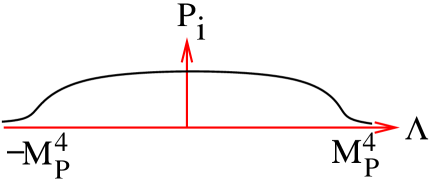
Now we must make contact with the cosmological constant, whose value locally depends on which of the many minima a given subuniverse finds itself in. Suppose there are $N$ which are accessible through classical evolution or tunneling. It is as good a guess as any to assume that the values of the minima of the potential, $V_{\rm min}$ are uniformly distributed over the range $\sim[-M_{p}^{4},M_{p}^{4}]$ with spacing $\Delta V\sim M_{p}^{4}/N$. If $N\mbox{\raisebox{-2.58334pt}{~{}$\stackrel{{\scriptstyle>}}{{\sim}}$~{}}}10^{120}$ then there will exist some vacua with $V_{\rm min}$ close to the observed value. The possible values of $\Lambda$ will be distributed according to some intrinsic probability distribution function $P_{i}(\Lambda)$ which depends on the details of the potential $V$, but in the absence of reasons to the contrary should be roughly uniform, as in b 3.

Fig. 3.: Intrinsic probability distribution for values of $\Lambda$ coming from minima of the landscape potential.

This theory explains why it is possible to find ourselves in a vacuum with the observed value of $\Lambda$. To understand why we were so lucky as to find it so unnaturally close to zero, we need to consider the conditional probability

$$P_{\rm tot}(\Lambda)=P_{i}(\Lambda)P_{\rm obs}(\Lambda)$$ (1.5)

where the second factor is the probability that an observer could exist in a universe with the given value of $\Lambda$. This part of the problem was considered by S. Weinberg originally in [5] in also in the review article [6] . In the abstract of the [5], he says that the anthropic bound on $\Lambda$ is too weak to explain the observed value of $\Lambda$, but in the later work he took the more positive view; living in a universe whose probability is 1% is far less puzzling than one where $P\sim 10^{-120}$. There are actually two anthropic bounds. For $\Lambda>0$, we must have $\Lambda\mbox{\raisebox{-2.58334pt}{~{}$\stackrel{{\scriptstyle<}}{{\sim}}$~{}}}10^{2}\Lambda_{\rm obs}$; otherwise the universe expands too quickly to have structure formation by redshifts of $z\sim 4$. For $\Lambda<0$, we need $\Lambda\mbox{\raisebox{-2.58334pt}{~{}$\stackrel{{\scriptstyle>}}{{\sim}}$~{}}}-\Lambda_{\rm obs}$ to avoid the recollapse of the universe before structure formation.

It is worth pointing out that this was a successful prediction of $\Lambda_{\rm obs}$ before it was determined to be nonzero through observations of distant supernovae [7]. From the anthropic point of view, there is no reason for $\Lambda$ to be zero, so its most natural value is of the same order of magnitude as the bound—assuming of course that $P_{i}$ is roughly uniform over the range where $P_{\rm obs}$ is nonnegligible.

1.3 The Bousso-Polchinski (Brown-Teitelboim) mechanism

We can now consider how the setting for this idea can be achieved within string theory. The most concrete example is due to Bousso and Polchinski [8], who found a stringy realization of the Brown-Teitelboim (BT) mechanism [9]. This is based on the existence of 4-form gauge field strengths $F^{(4)}_{\alpha\beta\gamma\delta}$ whose action is

$$S=\int d^{4}x\left[-\sqrt{-g}F^{(4)}_{\alpha\beta\gamma\delta}F_{(4)}^{\alpha\beta\gamma\delta}+8\partial_{\mu}\left(\sqrt{-g}F_{(4)}^{\mu\alpha\beta\gamma}A_{\alpha\beta\gamma}\right)\right]$$ (1.6)

leading to the equation of motion $\partial_{\mu}\left(\sqrt{-g}F_{(4)}^{\mu\alpha\beta\gamma}\right)=0$, with solution $F_{(4)}^{\mu\alpha\beta\gamma}=c\epsilon^{\mu\alpha\beta\gamma}$ where $c$ is a constant. The contribution to the action is

$$S=+\int d^{4}x\sqrt{-g}\,(-4!)\,c^{2}$$ (1.7)

The sign $+$ in front of the integral in (1.7) would have been $-$ had it not been for the total derivative term in (1.6) which must be there for consistency; otherwise the value of the vacuum energy appearing in the action has the opposite sign to that appearing in the equations of motion. This negative contribution to the action is a positive contribution to the vacuum energy density.

Although in field theory the constant $c$ is arbitrary, in string theory it is quantized. The particular setting used by Bousso and Polchinski is M-theory, which is 11 dimensional and has no elementary string excitations, but it does have M2 and M5 branes. The low-energy effective action for gravity and the 4-form is

$$S=2\pi M_{11}^{9}\int d^{11}x\sqrt{-g_{11}}\left(R-F_{(4)}^{2}\right)$$ (1.8)

The 4-form is electrically sourced by the M2-branes and magnetically sourced by the M5-branes, in a way which we will discuss shortly. To understand the quantization of $c$, it is useful to note that $F_{(4)}$ is Hodge-dual to a 7-form in 11 dimensions,

$$F_{(4)}=*F_{(7)}$$ (1.9)

(in terms of indices, this means contracting $F_{(7)}$ with the 11D Levi-Civita tensor). We can say that $F_{(7)}$ is electrically sourced by M5 branes. In the same way that electric charge in 4D is quantized if magnetic monopoles exist, there is a generalized Dirac quantization condition in higher dimensions which applies here because the wave function of an M5 brane picks up a phase when transported around an M2 brane, or vice versa. For the wave function to be single valued, it is necessary that the $F_{(7)}$ flux which is sourced by the M2 brane, when integrated over the 7D compactification manifold $K$, is quantized,

$$2\pi M_{11}^{6}\int_{K}F_{(7)}=2\pi n$$ (1.10)

This quantization also implies the quantization of $F_{(4)}$ through the duality relation (1.9). With this identification, we can evaluate the contribution to $\Lambda$ from (1.7) as

$$\Delta\Lambda=2n{(2\pi M_{11}^{3})^{2}\over 2\pi M_{11}^{9}V_{7}}={4\pi n\over M_{11}^{3}V_{7}}\sim{nM_{11}^{6}\over M_{p}^{2}}$$ (1.11)

where $V_{7}$ is the volume of $K$. This can be taken as the typical spacing between nearby values of the cosmological constant. Unfortunately, even if $M_{11}$ is as small as the TeV scale using large extra dimensions, one finds that $\Delta\Lambda/M_{p}^{4}\sim($TeV$/10^{15}$ TeV$)^{6}\sim 10^{-90}$, and this spacing is too large to solve the cosmological constant problem, which needs $10^{-120}$. In fact the problem is even worse, because if the bare value of $\Lambda$ which needs to be canceled is negative and of order $-M_{11}^{4}$, a large value of $n$ is required,

$$\Lambda_{\rm obs} = \Lambda_{\rm bare}+O\left({n^{2}M_{11}^{6}\over M_{p}^{2}}\right)$$ (1.12)

$$\Longrightarrow n\sim{M_{p}|\Lambda_{\rm bare}|^{1/2}\over M_{11}^{3}}$$

in which case $\Delta\Lambda/M_{p}^{4}\sim M_{11}^{3}|\Lambda_{\rm bare}|^{1/2}/M_{p}^{5}\sim 10^{-75}$ assuming $|\Lambda_{\rm bare}|\sim M_{11}^{4}$.

However, string theory has a nice solution to this problem. There is not just one 4-form, but one for each nontrivial 3-cycle in $K$. Then

$$F_{(7)}=*F_{(4,N+1)}\wedge\epsilon_{1}(y)+\sum_{i=1}^{N}F_{(4,i)}\wedge\omega_{3,i}(y)$$ (1.13)

where $F_{(4,N+1)}$ can be thought of as the original 4-form we started with, while $F_{(4,i)}$ is the $i$th additional one which arises for each nontrivial 3-cycle. Here $\epsilon_{1}(y)$ is the volume form on $K$ (whose coordinates are taken to be $y$) and $\omega_{3,i}(y)$ is the harmonic 3-form on the $i$th 3-cycle. There can easily be a large number of 3-cycles. For example if $K$ is a 7-torus, the number of inequivalent triples of 1-cycles is $({7\atop 3})=35$. If $K$ has more interesting topology the number can be larger. We no longer have a single flux integer $n$ but a high-dimensional lattice, $n_{i}$, such that

$$\Lambda_{\rm obs}=\Lambda_{\rm bare}+\frac{1}{2}\sum_{i}n_{i}^{2}q_{i}^{2}$$ (1.14)

where $q_{i}=M_{11}^{3/2}V_{3,i}/\sqrt{V_{7}}$ and $V_{3,i}$ is the volume of the $i$th 3-cycle. We can visualize a spherical shell in the space of the flux integers $n_{i}$, which is bounded by surfaces where $\Lambda=\Lambda_{\rm obs}$ and $\Lambda=\Lambda_{\rm obs}+\Delta\Lambda$, as illustrated in figure 4. As long as the lattice is fine enough so that at least one point is contained within the shell, then there exists a set of fluxes which can give a finely-enough tuned cancellation of $\Lambda_{\rm bare}$. The number of such lattice points is just the volume of the shell with radius $\sqrt{\frac{1}{2}\sum_{i}n_{i}^{2}q_{i}^{2}}=|\Lambda_{\rm bare}|^{\frac{1}{2}}$ and thickness $\Delta\Lambda^{\frac{1}{2}}\sim\Lambda_{\rm obs}^{\frac{1}{2}}$, in the $N$ dimensional space whose $i$th axis is the magnitude of $n_{i}q_{i}$. This fixes the magnitude of $q_{i}$ via

$${\Delta\Lambda\over M_{p}^{4}}\sim q_{i}^{N/2}\Gamma(N/2)\pi^{-N/2}$$ (1.15)

For example, if $N\sim 35$ we need $q_{i}\sim 10^{-3}$ while if $N\sim 100$, we need $q_{i}\sim 10^{-2/3}$. Let us suppose that the compactification and 3-cycle volumes are given in terms of a distance scale $R$, as $V_{7}\sim R^{7}$, $V_{3,i}\sim R^{3}$. Then

$$q_{i}\sim{M_{11}^{3/2}R^{-1/2}\over M_{p}^{2}}\sim{M_{11}^{3/2}R^{-1/2}\over M_{11}^{9}R^{7}}={1\over(M_{11}R)^{13/2}}$$ (1.16)

so the required small values of $q_{i}$ can be achieved by taking extra dimensions which are moderately larger than the fundamental distance scale.

Fig. 4.: Lattice of allowed 4-form flux integers, and a hyperspherical shell of values consistent with canceling a large negative $\Lambda_{\rm bare}$ to get a small $\Lambda_{\rm obs}$.

To complete the picture, we must describe how tunneling between the different vacuum states (labeled by the flux quanta) takes place. In the toy-model field-theory example, bubbles of the new vacuum phase with $\Lambda_{-}$ nucleate within the old one with $\Lambda_{+}$. In M-theory there is no scalar field, but we do have M2 and M5 branes. The M2 branes can serve as the walls of the bubbles since they are spatially two-dimensional, as illustrated in figure 5. Furthermore there is a natural way to couple the M2 branes to the 4-forms, which is a generalization of the coupling of a charged relativistic point particle to the Maxwell gauge field,

$$S=-\int d\tau J^{\mu}A_{\mu}$$ (1.17)

defined as an integral along the worldline of the particle, where $\tau$ is the proper time and $J^{\mu}=qdx^{\mu}/d\tau$. The generalization to strings is

$$S=-q\int d\tau d\sigma\,{\partial x^{\mu}\over\partial\tau}\,{\partial x^{\nu}\over\partial\sigma}\,A_{\mu\nu}$$ (1.18)

and for 2-branes it is

$$S=-q\int d\tau d\sigma_{1}d\sigma_{2}\,{\partial x^{\mu}\over\partial\tau}\,{\partial x^{\nu}\over\partial\sigma_{1}}\,{\partial x^{\rho}\over\partial\sigma_{2}}\,A_{\mu\nu\rho}$$ (1.19)

where $A_{\mu\nu}$ and $A_{\mu\nu\rho}$ are totally antisymmetric gauge potentials. This shows why M2-branes are sources of 4-form field strengths, since the latter are related to the 3-index gauge potential by

$$F_{(4)}=dA_{(3)},\quad F_{\mu\nu\alpha\beta}=A_{[\mu\nu\alpha,\beta]}$$ (1.20)

(the brackets indicate total antisymmetrization on the indices). Adding the Chern-Simons action (1.19) to the kinetic term for $F_{(4)}$ results in the equation of motion

$$\partial_{\mu}(\sqrt{-g}F^{\mu\nu\alpha\beta})=q\sum_{\mu}\delta^{(1)}(x^{\mu}-X^{\mu}(\tau,\sigma_{i}))\epsilon^{\mu\nu\alpha\beta}$$ (1.21)

For example if the M2 brane is in the $x$-$y$ plane and the spacetime is Minkowskian, then

$$\partial_{\mu}F^{\mu\nu\alpha\beta}=q\delta(z)\epsilon^{z\nu\alpha\beta}$$ (1.22)

whose solution is

$$F^{\mu\nu\alpha\beta}=\epsilon^{\mu\nu\alpha\beta}\left\{{c+q,\ z>0\atop c,\qquad z<0}\right.$$ (1.23)

Thus the value of the 4-form changes by the charge of the M2 brane when going from one side of the brane to the other.

Fig. 5.: Nucleation of bubble of new $\Lambda$ whose wall is an M2-brane.

In the BT mechanism, the value of $\Lambda$ decreases dynamically by the nucleation of bubbles whose surface has charge $q$ (figure 5). We now see why these bubble walls can be identified with the M2 branes of M-theory, which carry the quantized charge $q$. Having introduced a large number $N$ of 4-forms, we need to find separate sources with different charges $q_{i}$, one for each different $F_{(4,i)}$, yet M-theory only has one kind of M2 brane, with a unique charge. The source of the new $F_{(4,i)}$’s is the M5 brane, whose extra three dimensions can be wrapped on the different 3-cycles. Each one of these provides effectively a new kind of M2 brane. The fact that these branes must come in integer multiples also explains why the $F_{(4,i)}$ fluxes are quantized: since they are sourced by M2 branes, their strength must be proportional to the number of source branes. We can now better understand eq. (1.15): if we start from a situation with no fluxes and nucleate a stack of M2 branes, where $n_{i}$ copies of the $i$th kind of M2 brane are coincident, the new value of $F_{(4,i)}$ (after normalizing it in a convenient way) is given by $n_{i}q_{i}$, and the corresponding contributions to $\Lambda$ add in quadrature.

This construction establishes that string theory contains the necessary ingredients for realizing the original BT idea to explain the smallness of $\Lambda$. It is a concrete, detailed, and quantitative treatment, which gives a clear explanantion of how many closely-spaced values of $\Lambda$ can be generated. It is a nontrivial feat that it is possible to make the numbers work out favorably. There are also further hurdles to pass: the desired endpoint must have a lifetime greater than the age of the present universe since it is only metastable—this can be arranged since tunneling is typically exponentially suppressed—and the final universe (ours) must be born in an excited state so that inflation and reheating can take place subsequent to the nucleation. The latter requirement is less generic to satisfy, but possible, due to eternal inflation. If the inflaton is at an eternally inflating value during the tunneling, the daughter universe can also be eternally inflating. This puts a lower bound on $M_{11}$ around the GUT scale.

It is likely that other corners of the string theory parameter space can also provide settings for this basic idea. The theory we will focus on for inflation, type IIB string theory with flux compactification, gives exponentially large ($10^{\sim 500}$) numbers of vacua [10]. (See [11] for a discussion of the BTBP mechanism in this theory.)

It is worth emphasizing that the use of the anthropic principle is not merely optional once we accept the existence of many vacuum states. Unless there is a dynamical mechanism singling out one or a few of the possible states, we are forced to consider all of them, and then to restrict attention to those which satisfy the prior that observers can exist.

1.4 Caveats to the Landscape approach

It has been noted that the anthropic bound on $\Lambda$ is relaxed if the amplitude of density perturbations, $Q\sim 10^{-5}$ in our universe, is also allowed to vary [12]:

$$\hbox{bound on\ }\Lambda\sim Q^{3}$$ (1.24)

Rees and Tegmark argue that if $Q>10^{-4}$, galaxies would be too dense for life to evolve, which loosens Weinberg’s bound by a factor of $10^{3}$. Nevertheless, a one part in $10^{5}$ fine-tuning is much less daunting than one in $10^{120}$. Furthermore, there could be reasons for $Q$ not being “scanned” by the possible vacua of string theory, when we understand them better.

Another problem is the lack of additional predictions which would allow us to test whether the anthropic explanation is really the right one. However, we are still in the early days of understanding the landscape, so it may be premature to give up on making such predictions. Work along these lines is continuing at a steady pace [13, 14]. One hope is that by studying large anthropically allowed regions of the landscape, there might exist generic predictions for other quantities correlated with a small value of $\Lambda$, for example the scale of SUSY breaking. However the predictions are not yet clear, with some authors arguing for a small scale of SUSY breaking [15] while others suggest a high scale, for example the interesting possibility of “split SUSY,” in which all the bosonic superpartners are inaccessibly heavy and only the fermionic ones can be produced at low energies [16, 17]. In such scenarios the low Higgs mass would arise from the anthropic need for fine tuning instead of any mechanism like SUSY for suppressing the large loop contributions [13]. Unpalatable as some might find such a possibility, it is nonetheless a distinctive prediction, which if shown to be true would lend more weight to the landscape resolution of the cosmological constant problem.

2 Inflation

String theory brings some qualitatively new candidates for the inflaton, as well as some possible observable signatures that are distinct from typical field theoretic inflation. The inflaton could be the separation between two branes within the compact dimensions, or it could be moduli like axions associated with the Calabi-Yau (C-Y) compactification manifold. The new effects include large nongaussianity and inflation without the slow-roll conditions being satisfied, as in the DBI inflation scenario [18, 19]. There are also new issues connected with reheating in models with warped throats.

2.1 Brane-antibrane inflation

D$p$-branes in type II string theory are dynamical $(p+1)$-dimensional objects (with $p$ spatial dimensions) on which the ends of open strings can be confined, hence giving Dirichlet boundary conditions to the string coordinates transverse to the brane. There has been considerable progress in achieving stable compactifications within type IIB string theory in the last few years, using warped Klebanov-Strassler throats with fluxes [20, 21].

To put these developments into perspective, let us recall some differences between types of string theories. Type I theory describes both open and closed, unoriented strings with SO(32) gauge group. Its low energy effective theory is that of $N=1$ supergravity. Type II theories are of closed strings only (not counting the open string excitations which live on the D-branes themselves), with $N=2$ SUGRA effective theories. Type IIA theories contain D$p$-branes with $p$ even, while IIB contains odd-dimensional branes. Both of the type II theories have the same action from the NS-NS sector—the sector where the superpartners to the string coordinates $\psi^{\mu}$ have antiperiodic boundary conditions [22]:

$$S_{NS\hbox{-}NS}={1\over\kappa_{10}^{2}}\int d^{\,10}x\,\sqrt{-g}\,e^{-2\Phi}\left(R+4(\partial\Phi)^{2}-\frac{1}{2}|H_{3}|^{2}\right)$$ (2.1)

where $H_{3}$ is the 3-index Kalb-Ramond field strength, and $\Phi$ is the dilaton, which determines the string coupling via $g_{s}=e^{\Phi}$. The Ramond-Ramond (R-R) sector, where $\psi^{\mu}$ has periodic boundary conditions, exhibits the differences between type IIA and IIB theories:

$$S_{R\hbox{-}R}=-{1\over 4\kappa_{10}^{2}}\int d^{\,10}x\,\left\{\begin{array}[]{ll}|F_{2}|^{2}+|F_{4}|^{2},&IIA\\ |F_{1}|^{2}+|F_{3}|^{2}+\frac{1}{2}|F_{5}|^{2},&IIB\end{array}\right.$$ (2.2)

where $F_{n}$ is an $n$-index antisymmetric field strength. These expressions could have been written in a more symmetric way by including higher values of $n$, and taking coefficients of $\frac{1}{2}$ for each term, because of the duality relations

$$F_{6}=*F_{4},\quad F_{8}=*F_{2},\quad F_{5}=*F_{5},\quad{\it etc.}$$ (2.3)

$F_{n}$ couples to the D$p$-brane with $p=n-2$, as in eqs. (1.18, 1.19). Branes which have the wrong dimension for the theory in which they appear are unstable and quickly decay into closed strings.

The Chern-Simons couplings of the branes to the gauge fields show that branes are charged objects, and not simply delta-function sources of stress-energy as is often assumed in phenomenological brane-world models. This puts restrictions on the placement of branes within compact spaces. Since the gauge fields $F_{n}$ obey Gauss’ law, the net charge of the branes in the compact volume must vanish.

Consider for example a D3 brane parallel to a $\overline{\hbox{D3}}$ antibrane, which share parallel dimensions $x^{\mu}$ and are separated by a vector $y^{a}$ in the transverse directions, lying in the compact space. This is illustrated in figure 6. They are sources of $F_{5}$ through their Chern-Simons coupling, which can be more compactly written as

$$\sum_{i}\mu_{D_{3}}^{(i)}\int_{M_{4}^{(i)}}A_{4}$$ (2.4)

where $i$ labels the brane or antibrane having charge $\mu_{D_{3}}^{(i)}$ and world volume $M_{4}^{(i)}$. The equation of motion for $F_{5}$ is

$$\partial_{a}\left(\sqrt{-g}F^{a\alpha\beta\gamma\delta}\right)+\sum_{i}\mu_{D_{3}}^{(i)}\delta^{(6)}(y^{a}-y^{a}_{i})\epsilon^{\alpha\beta\gamma\delta}$$ (2.5)

where $a=5,\dots,9$ and $\alpha\beta\gamma\delta=0,1,2,3$ or some permutation. Integrating this over the compact dimensions gives

$$\int dF+\sum_{i}\mu_{D_{3}}^{(i)}=0$$ (2.6)

Since the integral must vanish, so must the sum of the charges.

Fig. 6.: Parallel D3 brane and $\overline{\hbox{D3}}$ antibrane.

We can also use Gauss’s law to find the force associated with the $F_{5}$ field, by considering noncompact extra dimensions, and integrating them over a 6D spherical region $R$ surrounding a single D3 brane. Then

$$\int_{R}dF_{5}=\int_{\partial R}F_{5}=|F_{5}|\times\left(\hbox{area of 5-sphere}\right)\sum\mu_{D_{3}}$$ (2.7)

This tells us that $|F_{5}|\sim\mu_{D_{3}}/r^{5}$ (the force) and $|A_{4}|\sim\mu_{D_{3}}/r^{4}$ (the potential), analogous to the $1/r$ Coulomb potential in 3D.

Similarly, the gravitational potential for a D3 brane goes like $1/r^{4}$, so the total potential for a D3-D3 or D3-$\overline{\hbox{D3}}$ system with separation $r$ in the compact dimensions is

$$V_{\rm tot}={G_{10}\over\frac{1}{4}\pi^{2}r^{4}}\left(-\tau_{3}^{2}\pm{\mu_{3}^{2}\over g_{s}^{2}}\right)\left\{{\hbox{upper sign for D3-D3}\atop\hbox{lower sign for D3-$\overline{\hbox{D3}}$}}\right.$$ (2.8)

where $\tau_{3}$ is the tension, generally given by

$$\tau_{p}={M_{s}^{p+1}\over(2\pi)^{p}g_{s}}$$ (2.9)

for a D$p$-brane, $M_{s}$ is the string mass scale, the 10D Newton constant is given by $G_{10}=(2\pi)^{6}g_{s}^{2}/(8M_{s}^{8})$, and the charge is related to the tension by $\mu_{p}=g_{s}\tau_{p}$. Because of this, the potential vanishes for D3-D3, but not for D3-$\overline{\hbox{D3}}$. We now consider whether this potential can be used to drive inflation.

We would like to use the distance $r$ between D3 and $\overline{\hbox{D3}}$ as the inflaton. This indeed is a field, since the branes are not perfectly rigid objects, but have transverse fluctuations. Hence at any longitudinal position $x^{\mu}$, the distance between the brane and antibrane is

$$r(x^{\mu})=\left(\sum_{a}\left(y^{a}(x^{\mu})-\bar{y}^{a}(x^{\mu})\right)^{2}\right)^{1/2}$$ (2.10)

We know the potential for $r$ from (2.8); all that remains is to determine its kinetic term. This is the Dirac-Born-Infeld (DBI) action which for a D$p$-brane in Minkowski space is

$$S=-\tau_{p}\int d^{\,p+1}x\,\left|\det\left(\eta_{\mu\nu}+\partial_{\mu}y^{a}\partial_{\nu}y^{a}\right)\right|^{1/2}$$ (2.11)

in coordinates where $x^{0},\dots,x^{p}$ are in the world-volume of the brane and $a=p+1,\dots,9$ label the transverse coordinates.

For inflation we are interested in homogeneous backgrounds where $y^{a}=y^{a}(t)$ and so

$$\eta_{\mu\nu}+\partial_{\mu}y^{a}\partial_{\nu}y^{a}={\rm diag}\left(-1+\sum_{a}(\dot{y}^{a})^{2},\ +1,\ \dots,\ +1\right)$$ (2.12)

Hence

$$|\det(\eta_{\mu\nu}+\partial_{\mu}y^{a}\partial_{\nu}y^{a})|^{1/2}=\sqrt{1-\sum_{a}(\dot{y}^{a})^{2}}$$ (2.13)

In the limit of small velocities we can Taylor-expand the square root to get the kinetic part of the action into the form

$$S=\frac{1}{2}\tau_{p}\sum_{a}(\dot{y}^{a})^{2}+O(\dot{y}^{4})$$ (2.14)

It follows that the canonically normalized inflaton field is

$$\phi=\sqrt{\tau_{3}}|\vec{y}-\vec{\bar{y}}|$$ (2.15)

and the Lagrangian for D3 brane-antibrane inflation becomes

$${\cal L}=\frac{1}{2}\dot{\phi}^{2}+2\left(\tau_{3}-{c\over\phi^{4}}\right)$$ (2.16)

where $c={4\over\pi^{2}}G_{10}\tau_{3}^{4}$. This should not be taken literally for $\phi^{4}<c/\tau_{3}$ however; the Coulomb-like potential is only a large-$r$ approximation. The energy density never becomes negative at small $r$. A more careful calculation shows that $V$ remains finite as $r\to 0$, but there a tachyonic instability occurs in another field when the brane-antibrane system reaches a critical separation [23]

$$y_{c}^{2}={2\pi^{2}\over M_{s}^{2}}$$ (2.17)

This is the separation at which the brane-antibrane system becomes unstable to annihilation into closed strings. The tachyon can be seen as the ground state of the string which stretches between the D3 and the $\overline{\hbox{D3}}$, whose mass is

$$m^{2}_{T}=M_{s}^{2}\left({y^{2}\over y_{c}^{2}}-1\right)$$ (2.18)

The full potential for $\phi$ and the tachyonic field $T$ resembles that of hybrid inflation, fig. 7.

Fig. 7.: The hybrid-like potential for the brane separation $\phi$ and the tachyon $T$.

Unfortunately, $V(\phi)$ is not flat enough to be suitable for inflation, unless the separation $r$ is greater than the size of the extra dimensions [24], an impossible requirement [25]. To see how this problem comes about, we compute the slow-roll parameters

$$\epsilon=\frac{1}{2}M_{p}^{2}\left({V^{\prime}\over V}\right)^{2}\cong\frac{1}{2}M_{p}^{2}\left({4c\over\tau_{3}\phi^{5}}\right)^{2}$$ (2.19)

$$\eta=M_{p}^{2}\,{V^{\prime\prime}\over V}\cong-M_{p}^{2}\,{20c\over\tau_{3}\phi^{6}}$$ (2.20)

where $M_{p}=2.4\times 10^{18}$ GeV $=(8\pi G_{N})^{-1/2}$. What is the relation between $G_{N}$ and $G_{10}$? This can be found by integrating out the extra dimensions from the 10D SUGRA action:

$$S_{NS\hbox{-}NS}={1\over 2\kappa_{10}^{2}g_{s}^{2}}\int d^{\,10}x\,\sqrt{-g_{10}}R_{10}\implies{1\over 16\pi G_{N}}\int d^{\,4}x\sqrt{-g}R$$ (2.21)

The coefficient of the 10D action can also be written as $(16\pi G_{10})^{-1}$, and after integrating over the extra dimensions, assumed to have volume $L^{6}$, the 10D integral becomes $L^{6}\int d^{\,4}x\sqrt{-g}R$. Hence

$${L^{6}\over G_{10}}={1\over G_{N}}$$ (2.22)

and

$$c={4\over\pi^{2}}L^{6}G_{N}\tau_{3}^{4}={L^{6}\tau_{3}^{4}\over 2\pi^{2}M_{p}^{2}}$$ (2.23)

This allows us to evaluate the slow-roll parameters as

$$\epsilon\sim{M_{s}^{24}L^{12}\over M_{p}^{2}\phi^{10}},\quad\eta\sim{M_{s}L^{6}\over\phi^{6}}$$ (2.24)

To get enough inflation, and to get the observed spectral index

$$n_{s}=2\eta-6\epsilon=0.95\pm 0.02$$ (2.25)

as observed by WMAP [26], it is necessary to have small values of $\epsilon$ and $\eta$. The condition $\eta<1$ is the more restrictive, and implies that the brane separation be

$$r=y\sim{\phi\over M_{s}^{2}}\gg L$$ (2.26)

which is the impossible situation of the branes being farther from each other than the size of the extra dimensions [25]. One can show that asymmetric compactifications do not help the situation. There were a number of attempts to solve this problem, but these could not be considered complete because of the additional unsolved problem of how to stabilize the moduli of the compactification. The early papers had to assume that the extra dimensions were stabilized somehow, in a way that would not interfere with efforts to keep the inflaton potential flat. However, this is a big assumption, as it later proved.

2.2 Warped Compactification

The problem of compactification was advanced significantly by Giddings, Kachru and Polchinski (GKP) [21], building on work of Klebanov and Strassler (KS) [20]. The KS construction involved putting branes at a conifold singularity, in order to reduce the number of supersymmetries of the effective action on the D3-brane world volume from $N=4$ down to the more realistic case of $N=1$. We need to understand this construction before studying its applications to inflationary model building.

The conifold is a 6D Calabi-Yau space, which can be described in terms of 4 complex coordinates $w_{i}$, constrained by the complex condition

$$\sum_{i=1}^{4}w_{i}^{2}=0$$ (2.27)

This looks similar to a cone, fig. 8 and the singularity is at the tip, where $w_{i}=0$. The base of the cone has the topology of $S_{2}\times S_{3}$, a 5D manifold. As one approaches the tip, the $S_{3}$ shrinks to a point, and the topology of the tip is the remaining $S_{2}$. The $S_{3}$ subspace is a 3-cycle, which is referred to as the A-cycle. There is also another (dual) 3-cycle, namely the $S_{2}$ times a circle which is extended along the radial direction, and which we call the B-cycle. The whole 6D manifold times 4D Minkowski space is a solution to Einstein’s equations in 10D, and so it is a suitable background for string theory.

Fig. 8.: The conifold and deformed conifold.

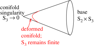
It is possible to deform the conifold so that it is no longer singular, by taking a more general condition than (2.27),

$$\sum_{i=1}^{4}w_{i}^{2}=z$$ (2.28)

Here $z$ is known as the complex structure modulus. For $z\neq 0$, the tip of the deformed conifold becomes a smooth point, at which the $S_{3}$ is no longer singular but has a size determined by $z$. The deformed conifold becomes the solution to Einstein’s equations when certain gauge fields of string theory are given nonzero background values. These are the RR field $F_{(3)}$ of type IIB theory, and the NS-NS Kalb-Ramond field $H_{(3)}$. Since they are 3-forms, they can have nonvanishing values when their indices are aligned with some of the 3-cycles mentioned above, similar to turning on an electric field along the 1-cycle (a circle) in the Schwinger model (electrodynamics in 1+1 dimensions). The lines of flux circulate and so obey Gauss’s law in this way. In a similar way to the 4-form flux of heterotic M-theory discussed in the previous section, these fluxes are also quantized, due to the generalized Dirac quantization argument. There are integers $M$ and $K$ such that

$${1\over 2\pi\alpha^{\prime}}\int_{A}F_{3}=2\pi M,\qquad{1\over 2\pi\alpha^{\prime}}\int_{B}H_{3}=-2\pi K$$ (2.29)

where the slope parameter $\alpha^{\prime}$ is related to the string mass scale by $\alpha^{\prime}=1/M_{s}^{2}$, and A,B label the 3-cycles mentioned above. It can be shown that these 3-cycles are specified by the conditions $\sum_{i=1}^{4}x_{i}^{2}=z$ for the A-cycle and $x_{4}^{2}-\sum_{i=1}^{3}y_{i}^{2}=z$ if $w_{n}=x_{n}+iy_{n}$. The size of the $S_{3}$ at the tip of the conifold gets stabilized by the presence of the fluxes; the complex structure modulus takes the value

$$z=e^{-2\pi K/(Mg_{s})}\equiv a^{3}(r_{0})$$ (2.30)

We will discuss the meaning of $a(r_{0})$ shortly.

When the fluxes are turned on, they also warp the geometry of the conifold. The line element for the full 10D geometry is

$$ds^{2}={dx^{\mu}dx_{\mu}\over\sqrt{h(r)}}+\sqrt{h(r)}\left(dr^{2}+r^{2}ds^{2}_{T_{1,1}}\right)$$ (2.31)

which is approximately AdS${}_{5}\times T_{1,1}$. The factor $T_{1,1}$ is the 5D base of the cone, known as an Einstein-Sasaki space, which for our purposes is some compact angular space whose details will not be important. The warp factor $h(r)$ is approximately of the form

$$h(r) = {R^{4}\over r^{4}}\left(1+g_{s}{M\over K}\times(\ln r\hbox{\ correction})\right)$$ (2.32)

$$\cong {R^{4}\over r^{4}},\qquad R^{4}={27\over 4}\pi g_{s}N\alpha^{\prime 2},\quad N=MK$$

This is a stringy realization of the Randall-Sundrum (RS) model [27], known as the Klebanov-Strassler throat, where the bottom of the throat (the tip of the conifold) is at $r=r_{0}$, such that

$${r_{0}\over R}=z^{1/3}=a(r_{0})=\hbox{\ warp factor}$$ (2.33)

This explains the introduction of $a^{3}(r_{0})$ in (2.30). The approximation $h=(R/r)^{4}$ gives the simple AdS₅ geometry for 4D Minkowski space times radial direction, and $R$ is the curvature scale of the AdS₅. The AdS part of the metric (2.31) can be converted to the RS form $ds^{2}=e^{\pm 2ky}dx^{2}+dy^{2}$ through the change of variables $dy=\mp(R/r)dr$, $y=\mp R\ln r$, $r=e^{\mp ky}$, where $k=1/R$. As shown in fig. 9, the top of the throat is understood to be smoothly glued onto the bulk of the greater Calabi-Yau manifold, whose geometry could be quite different from that of (2.31). The gluing is done at some radius $r\sim R$ where $h(r)\sim 1$.

Fig. 9.: The KS throat glued to the larger Calabi-Yau manifold where the radial coordinate $r\sim R$.

Let us take stock of what the fluxes have done for us before we continue with the search for inflation. First, they stabilized the complex structure modulus $z$, which without the fluxes was a massless field, with an undetermined value. In a similar way, they stabilize the dilaton, which is essential for any realistic string model since it determines the string coupling, and would give a ruled-out 5th force if massless. Second, they have given us warping, which introduces interesting possibilities for generating hierarchies of scales and generally having another parameter to tune.

Now we consider how the KS throat can be relevant for brane-antibrane inflation. We will see that a D3 brane by itself feels no force in the throat, whereas the $\overline{\hbox{D3}}$ antibrane sinks to the bottom. This is because of the combination of gravitational and gauge forces—they cancel for D3 but add for $\overline{\hbox{D3}}$. To understand how this comes about, recall that the D3 brane is the source of the $F_{(5)}$ field strength, which comes from the $C_{(4)}$ gauge potential. The fluxes create a background of $C_{(4)}$ or $F_{(5)}$ because there is contribution to the $F_{(5)}$ equation of motion (which we did not previously mention) of the form

$$dF_{5}\sim H_{3}\wedge F_{3}$$ (2.34)

Thus the complete action for a brane or an antibrane located at $r=r_{1}(x^{\mu})$ is

$$S=-\tau_{3}\int d^{\,4}x{1\over h(r_{1})}\sqrt{1-h(r_{1})(\partial r_{1})^{2}}\pm\tau_{3}\int d^{\,4}x(C_{4})_{0123}$$ (2.35)

where the sign is $+$ for D3 and $-$ for $\overline{\hbox{D3}}$. The form of the DBI part of the action can be understood from the more general definition,

$$S_{DBI}=-\tau_{3}\int d^{\,4}x\sqrt{-G}$$ (2.36)

where the induced metric on the D3-brane is given by

$$G_{\mu\nu}=G_{AB}{\partial X^{A}\over\partial x^{\mu}}{\partial X^{B}\over\partial x^{\nu}}={1\over\sqrt{h}}\eta_{\mu\nu}-\sqrt{h}\,\partial_{\mu}r\,\partial_{\nu}r$$ (2.37)

in the case where $r$ is the only one of the 6 extra dimensions which depends on $x^{\mu}$. Furthermore the equation of motion for the RR field has the solution

$$(C_{4})_{\alpha\beta\gamma\delta}={1\over h(r_{1})}\epsilon_{\alpha\beta\gamma\delta}$$ (2.38)

Consider the case where the transverse fluctuations of the brane vanish, $\partial r_{1}=0$. Then the two contributions to the action cancel for D3, but they add for $\overline{\hbox{D3}}$, to give

$$S=-2\tau_{3}\left({r_{1}\over R}\right)^{4}\int d^{\,4}x=-2\tau_{3}a^{4}(r_{1})\int d^{\,4}x$$ (2.39)

Notice that $\tau_{3}a^{4}$ is the warped brane tension, and $V=\tau_{3}a^{4}$ is the 4D potential energy associated with this tension. Because of the warp factor, $V$ is minimized at the bottom of the throat. This is why the antibrane sinks to the bottom of the throat, whereas the D3 is neutrally buoyant—it will stay wherever one puts it.

To be consistent, we should recall the words of warning issued earlier in these lectures: since branes carry charge, one is not allowed to simply insert them at will into a compact space. The background must be adjusted to compensate any extra brane charges. This results in a tadpole condition

$${\chi\over 24}=N_{D3}-N_{\overline{{D3}}}+{1\over\kappa_{10}^{2}T_{3}}\int_{C-Y}H_{3}\wedge F_{3}$$ (2.40)

where $\chi$ is the Euler number of the C-Y, and $N_{X}$ is the number of branes of type $X$. This relation says that for a fixed topology of the C-Y, any change in the net D3 brane charge has to be compensated by a corresponding change in the fluxes. The flux contribution is positive, so there is a limit on the net brane charge which can be accommodated, and this limit is determined by the Euler number, which can be as large as $\sim 10^{4}$ in some currently known C-Y’s.

2.3 Warped brane-antibrane inflation

With this background we are ready to think about brane-antibrane inflation in the KS throat, following KKLMMT [28]. Now we want to add not just a D3 or $\overline{\hbox{D3}}$ to the throat, but both together. To find the interaction energy requires a little more work relative to the calculation of (2.35). Following [28], we will consider how the presence of a D3 at $r_{1}$ perturbs the background geometry and $C_{4}$ field. Using the perturbed background in the action for the $\overline{\hbox{D3}}$ will then reveal the interaction energy. We can write the perturbation to the background as

$$h(r) \to h(r)+\delta h(r)$$ (2.41)

$$C_{4}(r) \to C_{4}(r)+\delta C_{4}(r)$$ (2.42)

where $\delta h$ is determined by the Poisson equation in 6D,

$$\nabla^{2}\delta h=C\delta^{(6)}(\vec{r}-\vec{r}_{1})$$ (2.43)

in analogy to the gravitational potential for a point mass in 4D; $C$ is a constant which turns out to have the value $C=R^{4}/N$ in terms of the AdS curvature scale and the product of flux quantum numbers. The solution is

$$\delta h={R^{4}\over Nr_{1}^{4}},\quad\delta C_{4}=-{\delta h\over h^{2}}$$ (2.44)

(see eq. (2.38)). Using the perturbed background fields, we can evaluate the Lagrangian for an antibrane at the bottom of the throat $r=r_{0}$, and expand to leading order in $(\partial r_{1})^{2}$, to find the result

$${\cal L} = \frac{1}{2}\tau_{3}(\partial r_{1})^{2}-2\tau_{3}\left({r_{0}\over R}\right)^{4}\left(1-\left({r_{0}\over R}\right)^{4}\,{R^{4}\over Nr_{1}^{4}}\right)$$ (2.45)

$$= \frac{1}{2}(\partial\phi)^{2}-2\tau_{3}a_{0}^{4}\left(1-a_{0}^{4}{R^{4}\tau_{3}^{2}\over N\phi^{4}}\right)$$ (2.46)

where we introduced the canonically normalized inflaton $\phi=\sqrt{\tau_{3}}r_{1}$ and $a_{0}=a(r_{0})$.

When we compute the slow roll parameters in the new theory with warping, and compare them to our previous calculation without the warp factors, we find that

$$\epsilon=a_{0}^{8}\,\epsilon_{\rm unwarped}$$

$$\eta=a_{0}^{4}\,\eta_{\rm unwarped}$$ (2.47)

Previously we had the problem that $\eta\sim 1$ unless the branes were separated by more than the size of the extra dimensions. With the new powers of $a_{0}$, we can easily make $\epsilon\ll\eta\ll 1$ since naturally $a\ll 1$. It looks like warping has beautifully solved the problem of obtaining slow roll in brane-antibrane inflation.

2.4 The $\eta$ problem

The story is that KKLLMMT had happily arrived at this result, but then realized the following problem. In fact $\eta$ is not small because one has neglected the effect of stabilizing the Kähler modulus (the overall size of the Calabi-Yau), $T$. The inflaton couples to $T$ in such a way that when a mass is given to $T$, it also inevitably gives a new source of curvature to the inflaton potential which makes $\eta$ of order unity. This is the well-known $\eta$ problem of supergravity inflation models.

To appreciate this, it is useful to consider the low-energy effective SUGRA Lagrangian for the Kähler modulus,

$${\cal L} = G_{T\overline{T}}\partial_{\mu}T\partial^{\mu}\overline{T}-e^{K}\left(G^{T\overline{T}}\,D_{T}W\overline{D_{T}W}-3|W|^{2}\right)$$ (2.48)

$$\equiv G_{T\overline{T}}\partial_{\mu}T\partial^{\mu}\overline{T}-V_{F}$$

where $T=\rho+i\chi$ is the complex Kähler modulus, related to the size $L$ of the Calabi-Yau through

$$\rho\equiv e^{4u}\sim L^{4},$$ (2.49)

$\chi$ is the associated axion,

$$G_{T\overline{T}}=\partial_{T}\partial_{\overline{T}}K$$ (2.50)

is the Kähler metric,

$$K=-3\ln(T+\overline{T})$$ (2.51)

is the Kähler potential, $W(T)$ is the superpotential,

$$D_{T}W=\partial_{T}W+W\partial_{T}K$$ (2.52)

is the covariant derivative of $W$, and $V_{F}$ is the F-term potential.

In the GKP-KS flux compactification, $T$ remains unstabilized because the fluxes generate a superpotential which only depends on the dilaton and complex structure modulus, not on $T$. Once these heavy fields are integrated out, $W$ can be treated as a constant, $W_{0}$. Then

$$D_{T}W = W\partial_{T}K=-3\,{W\over T+\overline{T}},$$ (2.53)

$$G_{T\overline{T}} = {3\over(T+\overline{T})^{2}},\quad G^{T\overline{T}}={(T+\overline{T})^{2}\over 3},$$ (2.54)

$$V_{F} = 3|W|^{2}-3|W|^{2}=0$$ (2.55)

A SUGRA theory where this kind of cancellation occurs is called a no-scale model.

Of course having a massless Kähler modulus is unacceptable, for all the reasons mentioned in section 1.1. We need a nontrivial superpotential $W(T)$. We will come back to this. First we focus on the coupling which the inflaton—the position of the mobile D3-brane—has to $T$, which will lead to problems when we introduce $W(T)$. Since Kähler manifolds are complex, we can regard the position of the D3-brane in the 6 extra dimensions as being specified by 3 complex coordinates, which become three complex scalar fields,

$$\phi^{i}(x^{\mu}),\quad i=1,2,3$$ (2.56)

Previously we ignored the dependence on the angular directions in $T_{1,1}$ and only kept track of the radial position of the brane in the throat, $r$, but (2.56) is the more precise specification. It can be shown by several arguments (of which we will give one shortly) that when there is a D3 brane in the throat, it changes the Kähler potential by

$$K\to K\left(T+\overline{T}-k(\phi^{i},\bar{\phi}^{i})\right)\equiv K(2\sigma)$$ (2.57)

where $k(\phi^{i},\bar{\phi}^{i})$ is a real-valued function, known as the Kähler potential for the Calabi-Yau (not to be confused with $K$ which is the Kähler potential for the field space). Now it is the combination $2\sigma$ and not $T+\overline{T}$ which is related to the physical size of the Calabi-Yau,

$$2\sigma=L^{4}=e^{4u}=V^{2/3}$$ (2.58)

where $V$ is the volume of the extra dimensions. It can be shown (see for example [29]) that

$$k=\sum_{i}\phi^{i}\bar{\phi}^{i}+O(\phi^{4})$$ (2.59)

in the vicinity of the bottom of the throat, labeled by $\phi^{i}=0$. (KKLMMT did not make this identification of $\phi^{i}=0$ with the bottom of the throat.)

Next we can generalize the SUGRA action to take account of the additional brane moduli fields, writing

$${\cal L}=G_{I\overline{J}}\partial_{\mu}\Phi^{I}\partial^{\mu}\overline{\Phi}^{J}-e^{K}\left(G^{I\overline{J}}D_{I}W\overline{D_{J}W}-3|W|^{2}\right)$$ (2.60)

where $\Phi^{I}=(T,\phi^{i})$. One can show that the new definition of $K$ still leads to a no-scale model if $W$ is constant, so $V_{F}$ remains zero in the presence of the D3 brane. However the kinetic term is modified; the Kähler metric for the brane moduli is

$$G_{i\bar{\jmath}} = {\partial^{2}K\over\partial\phi^{i}\partial\bar{\phi}^{j}}={\partial\over\partial\bar{\phi}^{j}}\left({3\bar{\phi}^{i}\over T+\overline{T}-k}\right)$$

$$= {3\delta_{ij}\over 2\sigma}+{3\phi^{j}\bar{\phi}^{i}\over 2\sigma}$$

where the last term is considered to be small because we want $\sigma$ to be large to justify integrating out the extra dimensions (so that the corrections from higher dimension operators involving the curvature are small), and this requires that $\phi^{2}\ll T+\overline{T}$. Then the kinetic term in the Lagrangian is

$${\cal L}_{\rm kin}\cong{3\over 2\sigma}\left|\partial_{\mu}\phi^{i}\right|^{2}$$ (2.62)

To justify the replacement (2.57), we can derive the kinetic term of the brane modulus by a different method, using the DBI action for the brane [30]. For this, we need the form of the 10D metric that includes not only warping, but also the dependence on the Kähler modulus Re($T)=e^{4u}$:

$$ds^{2}={e^{-6u}\over\sqrt{h}}dx^{2}+e^{2u}\sqrt{h}\,\tilde{g}^{(6)}_{ab}dy^{a}dy^{b},$$ (2.63)

where $\tilde{g}^{(6)}_{ab}$ is the metric with some fiducial volume on the C-Y. The factor $e^{2u}$ in the 6D part of the metric is understandable since $e^{u}\sim L$; the corresponding factor $e^{-6u}$ in the 4D part is there to put the metric in the Einstein frame, where there is no mixing of the Kähler modulus with the 4D graviton. We can now compute the induced metric in the D3 world-volume,

$$G_{\mu\nu}=G_{AB}\,{\partial X^{A}\over\partial\sigma^{\mu}}\,{\partial X^{B}\over\partial\sigma^{\nu}}={e^{-6u}\over\sqrt{h}}\eta_{\mu\nu}-e^{2u}\sqrt{h}\,\tilde{g}^{(6)}_{ab}{\partial X^{a}\over\partial\sigma^{\mu}}\,{\partial X^{b}\over\partial\sigma^{\nu}}$$ (2.64)

Using this in the DBI Lagrangian and Taylor-expanding in the transverse fluctuations, we find that

$$-\tau_{3}\sqrt{|G_{\mu\nu}|}=-a^{4}\tau_{3}+{3\tau_{3}\over 4\sigma}(\partial_{\mu}X^{a})^{2}+O((\partial X)^{4})$$ (2.65)

where $a$ is the value of the warp factor at the position of the brane. This reveals the presence of the extra factor of $1/\sigma$ in the brane kinetic term which we did not see previously when we were only considering the effect of warping, and it justifies the SUGRA description given above. We see that the SUGRA and DBI fields are identified through

$$\phi^{1}=\sqrt{3\tau_{3}\over 2\sigma}(X_{1}+iX_{2}),\hbox{\it\ etc.}$$ (2.66)

With this background we can now present the $\eta$ problem. As long there is no potential for $T$, no new potential is introduced for the inflaton $\phi^{i}$; however we know that a stabilizing potential for $T$ must be present. Several ways of nonperturbatively generating such a potential were suggested by KKLT [31], which yield an extra contribution to the superpotential,

$$W=W_{0}+Ae^{-aT}$$ (2.67)

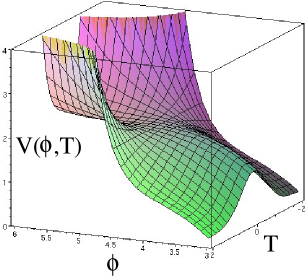
By itself, this new contribution indeed stabilizes $T$ at a nontrivial value, but at the minimum the potential $V_{0}$ is negative, as shown in fig. 10, which would give an AdS background in 4D, rather than Minkowski or de Sitter space. To lift $V_{0}$ to a nonnegative value, one needs an additional, supersymmetry-breaking contribution, which thus appears directly as a new contribution to the potential rather than to the superpotential. In fact, placing a $\overline{\hbox{D3}}$ antibrane in the throat does precisely what is needed. As we have already seen, a $\overline{\hbox{D3}}$ has positive energy, twice the warped tension, due to the failure of cancellation of the gravitational and RR potentials. It is minimized at a nonzero value when the $\overline{\hbox{D3}}$ sinks to the bottom of the throat. The important point is that in the Einstein frame, taking into account the Kähler modulus, the $\overline{\hbox{D3}}$ contribution to the potential takes the form

$$\delta V={2a_{0}^{4}\tau_{3}\over(2{\rm Re}T)^{2}}$$ (2.68)

However we have seen that when a D3 brane is in the throat, it modifies the volume of the C-Y, and we must replace 2Re$T\to 2\sigma=T+\overline{T}-|\phi|^{2}$. In addition, we get the Coulombic interaction energy between the brane and the antibrane so the total inflaton potential becomes

$$\delta V\to{V(\phi)\over(2\sigma)^{2}}\cong{2a_{0}^{4}\tau_{3}}{1-c|\phi|^{-4}\over(T+\overline{T}-|\phi|^{2})^{2}}$$ (2.69)

Fig. 10.: The KKLT potential for the Kähler modulus, before uplifting by $\overline{\hbox{D3}}$ antibrane.

The $\eta$ problem is now apparent, since even if the Coulomb interaction is arbitrarily small ($c\to 0$), the inflaton gets a large mass from the term in the denominator:

$${\cal L}\sim{3\over 2\sigma}(\partial\phi)^{2}-{a_{0}^{4}\tau_{3}\over 2\sigma^{2}}\left(1+{|\phi|^{2}\over\sigma}\right)$$ (2.70)

We see that the inflaton mass is of order the Hubble parameter,

$$m^{2}=\frac{2}{3}V=2H^{2}$$ (2.71)

(working in units where $M_{p}=1$), which implies that $\eta=V^{\prime\prime}/V=m^{2}/(3H^{2})=2/3$, whereas inflation requires that $\eta\ll 1$. This is the $\eta$ problem.

2.5 Solutions (?) to the $\eta$ problem

A number of possible remedies to the flatness problem of brane-antibrane inflation have been suggested. We will see that many of these have certain problems of their own.

2.5.1 Superpotential corrections

In an appendix of [28], the possibility of having $\phi$-dependent corrections to the superpotential was discussed,

$$W=W_{0}+Ae^{-aT}(1+\delta|\phi|^{2})$$ (2.72)

which is just an ansatz for the kind of corrections which might arise within string theory. The inflaton mass from this modified superpotential was computed to be

$$m^{2}=2H^{2}\left(1-{|V_{\rm AdS}|\over V_{dS}}(\beta-2\beta^{2})\right)$$ (2.73)

where $\beta=-\delta/a$, and $V_{\rm AdS}$ is the value of the potential at the AdS minimum, before uplifting with the antibrane. By fine-tuning $\beta$, one can make $m^{2}\ll H^{2}$ and thus get acceptable inflation. (It was argued in [32] that the tuning is only moderate, but this seems to be contingent upon taking 3$\sigma$ rather than 1$\sigma$ error bars from the experimental constraints.) The suggestion of using superpotential corrections was made before any concrete calculations of the actual corrections had been carried out. Since then, it has been shown that they have a form which drive the brane more quickly to the bottom of the throat rather than slowing it down; the corrections have the wrong sign [33, 34].

2.5.2 Tuning the length of the throat

In KKLMMT, the impression was given that the function $k(\phi,\bar{\phi})=|\phi|^{2}+O(\phi^{4})$ was expanded around some point in the C-Y which did not necessarily coincide with the bottom of the throat; in their calculation it did not matter where this point was because they assumed the Coulomb part of the potential was negligible compared to the dependence via $T+\overline{T}-k(\phi,\bar{\phi})$. However, if the origin of $\phi^{i}$ was assumed to be at a position other than the bottom of the throat, thus located at some position $\phi_{0}$, then there could be a competing effect between the two sources of $\phi$-dependence, which when properly tuned could lead to a flat potential without invoking superpotential corrections. The full potential then had the form [35]

$${\cal L}={3T\over(2T-\phi^{2})^{2}}(\partial\phi)^{2}-{2\tau_{3}a_{0}^{4}\over(2T-\phi^{2})^{2}}\left(1+{a_{0}^{4}\over N(\phi-\phi_{0})^{4}}\right)^{-1}$$ (2.74)

where (recall that) $N=JK$ is the product of the flux quantum numbers, and we have displayed the potential in a form which makes sense even as $\phi\to\phi_{0}$ (whereas keeping only the first term of the Taylor expansion does not). By tuning $\phi_{0}$ we can adjust the flatness of the potential in the region between $\phi=0$, assumed to be somewhere near the top of the throat, and $\phi=\phi_{0}$, the bottom. Figure 11 shows the effect of changing the value of $\phi_{0}$ relative to other dimensionful combinations of parameters in the potential.

Fig. 11.: The brane-antibrane potential for different values of $\phi_{0}$ relative to other parameters in the potential.

Unfortunately, the same computations [33, 34] which clarified the nature of the superpotential corrections also made it clear that $\phi=0$ indeed corresponds to the bottom of the throat, so $\phi_{0}$ is not a free parameter which can be tuned. However there is a related idea that appears to be viable. Suppose there are two throats, related to each other by a $Z_{2}$ symmetry. A brane in between them would not be able to decide which throat to fall into, so the potential must be flat at this point in the middle [36].

2.5.3 Multibrane inflation

It was also suggested that instead of using a single D3-$\overline{\hbox{D3}}$ pair, one can use stacks of $M$ D3-branes and $M$ $\overline{\hbox{D3}}$-branes. If the branes in each stack are coincident, the Lagrangian becomes

$${\cal L}={\cal L}=M{3T\over(2T-M\phi^{2})^{2}}(\partial\phi)^{2}-M{2\tau_{3}a_{0}^{4}\over(2T-M\phi^{2})^{2}}\left(1+M{a_{0}^{4}\over N(\phi-\phi_{0})^{4}}\right)^{-1}$$ (2.75)

In [37] it was shown that the shape of the potential can vary with $M$ in such a way that for large $M$ there is a metastable minimum in which the brane stacks remain separated, while for small $M$ the minimum becomes a maximum (fig. 12). For an intermediate value of $M$, the potential is nearly flat. The interesting feature is that $M$ can change dynamically by tunneling of branes from the metastable minimum through the barrier to the stack of antibranes. In this way one could eventually pass through a nearly flat potential suitable for inflation. Unfortunately this mechanism also relied on the parameter $\phi_{0}$ which was shown to be zero.

Fig. 12.: The brane-antibrane potential for different values of $M$, the number of branes or antibranes in each stack.

One might have hoped that even without the possibility of tuning, having $M$ branes in the stack could allow for assisted inflation [38], where the slow-roll parameters get reduced by a factor of $M$ if all inflatons are rolling in the same way. Unfortunately this mechanism only works if the potential for each field by itself is independent of $M$. In the potential (2.75), this is not the case: the $V^{\prime\prime}/V$ also increases with $M$, undoing the assistance which would have come from renormalizing the field to get a standard kinetic term. On the other hand, ref. [39] finds that assisted inflation does work for multiple M5 branes moving along the 11th dimension of M-theory.

2.5.4 DBI inflation (D-celleration)

References [18, 19] explored a different region of the brane-antibrane parameter space and exposed a qualitatively new possibility, in which fast roll of the D3 brane could still lead to inflation. In this regime, one does not expand the DBI action in powers of $\dot{\phi}^{2}$ since it is no longer considered to be small. The Lagrangian has the form

$${\cal L}=-a^{3}(t)\left({\tau_{3}\over h(r)}\sqrt{1-h(r)\dot{r}^{2}}-V(r)\right)$$ (2.76)

where $a(t)$ is the scale factor and $r$ is the radial position of the D3-brane in the throat. To be in the qualitatively new regime, one wants the potential to be so steep that the brane is rolling nearly as fast as the local speed limit in the throat, beyond which the argument of the square root changes sign: $h(r)\dot{r}^{2}\sim 1$. One finds that this results in power-law inflation,

$$a(t)\propto t^{1/\epsilon},\quad\epsilon\cong{M_{p}\over m}\,\sqrt{3g_{s}\over R^{4}M_{s}^{4}}$$ (2.77)

where we recall that $R$ is the AdS curvature scale of the throat, $M_{s}$ is the string scale, and $m$ is the inflaton mass. One sees that inflation works best when $m$ is as large as possible, which is quite different from inflation with a conventional kinetic term. Even if $m\ll M_{p}$, we can compenstate by taking $R\gg M_{s}^{-1}$ to get $\epsilon\ll 1$.

However, this takes a huge amount of flux in the original KS model. Recall that $R^{4}M_{s}^{4}={27\pi\over 4}g_{s}N$ where $N=JK$, so

$$\epsilon={M_{p}\over m}\sqrt{4\over 9\pi N}$$ (2.78)

If $m$ is of order the GUT scale, then we need $J\sim K\sim 10^{3}$. In fact the problem is even worse, because the COBE normalization of the CMB power spectrum gives

$$P={1\over 4\pi^{2}}\,{g_{s}\over\epsilon^{4}\lambda}$$ (2.79)

where $\lambda=R^{4}M_{s}^{4}$ is identified as the ‘t Hooft coupling in the context of the AdS-CFT correspondence. The COBE normalization implies that $\lambda\sim 10^{14}$, which requires an Euler number for the C-Y of the same order, according to the tadpole condition (2.40). This exceeds by many orders of magnitude the largest known example. Ref. [19] suggests some ways to overcome this difficulty.

One of the most interesting consequences of DBI inflation is the prediction of large nongaussianity, which is not possible in conventional models of single-field inflation. To see why it occurs in the DBI model, one should consider the form of the Lagrangian for fluctuations $\delta\phi$ of the inflaton. The unperturbed kinetic term has the form

$${\cal L}_{\rm kin}=-{1\over h}\sqrt{1-h\dot{\phi}^{2}}\equiv{1\over h\gamma}$$ (2.80)

where $\gamma$ is analogous to its counterpart in special relativity; in the DBI inflation regime, we have $\gamma\gg 1$ since the field is rolling close to its maximum speed. The first variation of this term is

$$\delta{\cal L}_{\rm kin} = {1\over h}\,{h\dot{\phi}\over\sqrt{1-h\dot{\phi}^{2}}}\,\delta\dot{\phi}=\gamma\dot{\phi}\delta\dot{\phi}$$ (2.81)

$$\cong {\gamma\over\sqrt{h}}\,\delta\dot{\phi}$$

The fluctuation Lagrangian is enhanced relative to the zeroth order Lagrangian by powers of $\gamma$. The higher the order in $\delta\phi$, the more powers of $\gamma$. Nongaussian features start appearing at order $\delta\phi^{3}$, through the bispectrum (3-point function) of the fluctuations. DBI inflation predicts that the nonlinearity parameter, which is the conventional measure of nongaussianity, is of order

$$f_{NL}\cong 0.06\gamma^{2}$$ (2.82)

which is $\gamma^{2}$ times the prediction of ordinary inflation models. The current experimental limit is $|f_{NL}|\mbox{\raisebox{-2.58334pt}{~{}$\stackrel{{\scriptstyle<}}{{\sim}}$~{}}}100$ [26], (hence $\gamma<40$), with a future limit of $|f_{NL}|\mbox{\raisebox{-2.58334pt}{~{}$\stackrel{{\scriptstyle<}}{{\sim}}$~{}}}5$ projected for the PLANCK experiment. Thus DBI inflation has a chance of producing observable levels of nongaussianity, which conventional models do not.

Moreover, DBI inflation predicts a tensor component of the CMB with tensor-to-scalar ratio

$$r=16{\epsilon\over\gamma}$$ (2.83)

so that an upper bound on nongaussianity (hence on $\gamma$) implies a lower bound on tensors—a kind of no-lose theorem.

The original work on DBI inflation focused on inflation far from the tip of the throat, but recent work has pointed out that generically (for the KS throat background) one tends to get the last 60 e-foldings of inflation at the bottom the throat, and having larger-than-observed levels of nongaussianity [40].

2.5.5 Shift symmetry; D3-D7 inflation

It was suggested [41] that there could be a symmetry of the Lagrangian

$$\phi_{i} \to \phi_{i}+c_{i}$$ (2.84)

$$T \to \bar{c}_{i}\phi_{i}+\frac{1}{2}\sum c_{i}\bar{c}_{i}$$ (2.85)

which leaves a flat direction despite the combination $T+\overline{T}-|\phi|^{2}$ in the Kähler potential. In fact, it is only necessary to preserve a remnant of this shift symmetry, $\phi_{i}\to\phi_{i}+$ Re($c_{i})$ to get a flat inflaton potential; this can be achieved with a superpotential of the form

$$W=W_{0}+Ae^{-a(T-\frac{1}{2}\phi^{2})+i\beta_{i}\phi_{i}}$$ (2.86)

Such a symmetry requires an underlying symmetry of the compactification manifold, namely isometries, which would exist for toroidal compactifications. These are not favored for realistic model building.

It was argued that shift symmetry can occur in models where inflation is driven by the interaction between a D3 and a D7 brane [42]. It is interesting to note that the DBI action for D7-branes does not get the factor of $1/\sigma$ which was the harbinger of the $\eta$ problem for D3-$\overline{\hbox{D3}}$ inflation. If we split the C-Y metric into two factors $\tilde{g}^{(4)}$ for the extra dimensions parallel to D7, and $\tilde{g}^{(2)}$ for those which are transverse, the induced metric for D7 gives

$$\sqrt{G_{ab}} \cong \sqrt{g^{(4)}\tilde{g}^{(2)}}\,\left(1-g_{(4)}^{\mu\nu}\,\tilde{g}^{(2)}_{ij}\,\partial_{\mu}S^{i}\partial_{\nu}S^{j}\right)^{1/2}$$ (2.87)

$$\sim (e^{-6u+2u})^{4/2}\left(1-\frac{1}{2}e^{6u+2u}(\partial S)^{2}\right)$$

and the factors of $u$ cancel out of the kinetic term for the two transverse fluctuations $S^{i}$.

D3-D7 inflation can be pictured as a point (the D3 brane fully localized in the extra dimensions) interacting with a 4-brane (the 4 dimensions of the D7 which wrap the compact dimensions), which is like a D3 smeared over 4 extra dimensions. Thus the $1/r^{4}$ Coulombic potential of D3-$\overline{\hbox{D3}}$ gets integrated over 4 dimensions to become a logarithmic potential for D3-D7. This potential arises from SUSY-breaking effects, such as turning on fluxes which live in the world-volume of the D7-brane.

The low-energy description of this model is a SUGRA hybrid inflation model, with potential

$$V(S,\phi_{+},\phi_{-}) = 2g^{2}|S|^{2}(|\phi_{+}|^{2}+|\phi_{-}|^{2})+2g^{2}\left|\phi_{+}\phi_{-}-\frac{1}{2}\zeta_{+}\right|^{2}$$ (2.88)

$$+ \frac{1}{2}g^{2}\left(|\phi_{+}|^{2}-|\phi_{-}|^{2}-\zeta_{3}\right)^{2}$$

where $S$ is the brane separation in a $T^{2}/Z_{2}$ subspace of the C-Y, $\phi_{\pm}$ are the lowest modes of the strings stretched between D3 and D7, and $\zeta_{3}$, $\zeta_{+}$ are Fayet-Iliopoulos terms, which arise due to a background Kalb-Ramond $H_{3}$ field strength.

$S$ is the inflaton, while the fields $\phi_{\pm}$ are “waterfall” fields, whose tachyonic instability brings about the end of inflation, provided that $\zeta_{3}$ or $\zeta_{+}\neq 0$. In that case $m^{2}_{\phi_{\pm}}$ changes sign as $S\to 0$. The instability is the dissolution of the D3 in the D7. At large $S$, the waterfall fields’ potentials are minimized at $\phi_{\pm}=0$, and the potential for $S$ is exactly flat (as demanded by the shift symmetry). However SUSY-breaking generates a potential for $S$ at one-loop,

$$\Delta V={g^{4}\over 16\pi^{2}}\zeta_{3}^{2}\ln\left|S\over S_{c}\right|^{2}$$ (2.89)

as is needed to get inflation to end. However it is still an open question as to whether the shift symmetry gets broken more badly than this, possibly spoiling inflation, when the full quantum corrections are taken into account [43].

2.5.6 Racetrack and Kähler moduli inflation

Another alternative is to get rid of the mobile D3-brane entirely and instead use the compactification moduli to get inflation [44]. This requires a slightly more complicated superpotential

$$W=W_{0}+Ae^{-aT}+Be^{-bT}$$ (2.90)

which for historical reasons is known as a racetrack superpotential. It can come about from gaugino condensation in two strongly interacting gauge groups, e.g. SU(N)$\times$SU(M), giving $a=2\pi/N$, $b=2\pi/M$. Another possibility is to have two different Kähler moduli [45], with

$$W=W_{0}+Ae^{-aT_{1}}+Be^{-bT_{2}}$$ (2.91)

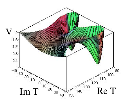
The latter form arises from a a very specific C-Y compactification [46]; hence this model is rigorously based on string theory. By fine tuning parameters, one can find a saddle point such that the axionic direction Im$T$ (or a linear combination of them in the case where there are two Kähler moduli) is flat and gives rise to inflation. The potential is shown in fig. 13. Interestingly, both models (2.90, 2.91) seem to point to a spectral index of $n_{s}=0.95$, in agreement with the recent WMAP measurement. Getting a flat enough spectrum however also seems to require uncomfortably large values for the rank of the gauge group(s). A positive feature of the model is that the existence of degenerate minima leads to inflating domain walls, an example of topological inflation, which solves the initial value problem: it is guaranteed that regions undergoing inflation will always exist in the universe, which are the borderlines between regions existing in the different vacua.

Fig. 13.: The potential for the Kähler modulus in a racetrack inflation model.

The fine-tuning problem of the simplest racetrack models can be overcome in backgrounds with a larger number of Kähler moduli [47]. In these models, the C-Y volume can naturally be quite large [48], and the potential can be flat since terms proportional to $e^{-aT_{i}}$ are small corrections in the large-$T_{i}$ regime, as long as there are some contributions to the potential which are not exponentially suppressed. Ref. [47] finds that this can be realized in models with three or more Kähler moduli, thus alleviating the need for fine tuning.

2.6 Confrontation with experiment

Having described a few of the inflationary models which arise from string theory, let’s reconsider the experimental constraints which can be used to test them.

2.6.1 Power spectrum

The scalar power spectrum of the inflaton is the main connection to observable physics. It is parametrized as

$$P(k)=A_{s}\left({k\over k_{0}}\right)^{n_{s}-1}$$ (2.92)

where currently $A_{s}=4\times 10^{-10}$ if $k_{0}=7.5a_{0}H_{0}$ (this is the COBE normalization [49]) and $n_{s}=0.95\pm 0.02$. For a single-field inflationary model $P(k)$ is predicted to be

$$P(k)={1\over 50\pi^{2}}\,{H^{4}\over\frac{1}{2}\dot{\phi}^{2}}$$ (2.93)

evaluated at horizon crossing, when $k/a=H$. Using the slow-roll equation of motion for the inflaton, $3H\dot{\phi}=V^{\prime}$, one can show that [49]

$$P(k)={V\over 150\pi^{2}\epsilon M_{p}^{4}}$$ (2.94)

Many of the inflation models we considered have noncanonically normalized kinetic terms; for example supergravity models typically have ${\cal L}_{\rm kin}\sim(\partial T/T)^{2}$. It is often useful to be able to evaluate quantities in the original field basis rather than having to change to canonically normalized fields. The correct generalization of (2.93) is simply

$$P(k)={1\over 50\pi^{2}}\,{H^{4}\over{\cal L}_{\rm kin}}$$ (2.95)

In addition to the scalar power, there is a tensor contribution to the temperature fluctuations, whose amplitude relative to the scalar contribution is

$$r={A_{t}\over A_{s}}=16\epsilon$$ (2.96)

in terms of the slow-roll parameter $\epsilon$ (but see the different prediction (2.83) from DBI inflation). The current limit is $r<0.3$ [26].

2.6.2 Numerical methods

Moreover in some models, like racetrack inflation, the inflaton is some combination of several fields, and it is useful to have an efficient way of numerically solving the equations of motion. Here is one approach. Let

$$\pi_{i}={\partial{\cal L}\over\partial\dot{\phi}_{i}}=f_{ij}(\phi)\dot{\phi}_{j}$$ (2.97)

which can be inverted algebraically to find $\dot{\phi}_{i}$ as a function of the canonical momenta. The equations of motion for the scalar fields are

$${d\over dt}\left(a^{3}\pi_{i}\right) = a^{3}{\partial\over\partial\phi_{i}}({\cal L}_{\rm kin}-V)$$

$$\implies\dot{\pi}_{i}+3H\pi_{i} = {\partial\over\partial\phi_{i}}({\cal L}_{\rm kin}-V)$$ (2.98)

This together with

$$\dot{\phi}_{i}=f_{ij}^{-1}\pi_{j}$$ (2.99)

constitute a set of coupled first order equations which can be numerically integrated along with the Friedmann equation which determines $a(t)$. However we are usually not interested in the actual time dependence of the solutions, but rather in the dependence on the number of e-foldings, $N=\int Hdt$. It is therefore more efficient to trade $t$ for $N$ using $dN=Hdt$, $H{d\over dN}={d\over dt}$. This makes it unnecessary to also solve the Friedmann equation, and one can simply transform the scalar field equations of motion to

$${d\pi_{i}\over dN}+3\pi_{i} = {1\over H}{\partial\over\partial\phi_{i}}({\cal L}_{\rm kin}-V)$$ (2.100)

$${d\phi_{i}\over dN} = {1\over H}f_{ij}^{-1}\pi_{j}$$ (2.101)

where

$$H=\sqrt{{\cal L}_{\rm kin}+V\over 3M_{p}^{2}}$$ (2.102)

Knowing $\phi_{i}(N)$ and $\pi_{i}(N)$, one can compute the power $P$ as a function of $N$, as shown in figure 14. The tilt at any point can be computed from

$$n_{s}-1={d\ln P\over d\ln k}={d\ln P\over dN}\left(1+H^{-1}{dH\over dN}\right)^{-1}\cong{d\ln P\over dN}$$ (2.103)

Here we used the horizon crossing condition $k=aH=e^{N}H$, hence $\ln k=N+\ln H$, $d\ln k=dN+d\ln H/dN$ to change variables from $k$ to $N$.

Fig. 14.: (a) Scalar power as a function of the number of e-foldings.

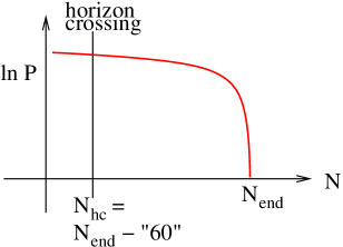
We are of course interested in evaluating the properties of the power spectrum at the COBE scale, when perturbations roughly of the size of the present horizon originally crossed the inflationary horizon. This occurs at an $N$ given by $N=N_{hc}$, nominally 60 e-foldings before the end of inflation. However when we say 60, this is an upper bound, determined by the maximum energy scale of inflation $M_{\rm inf}$ consistent with the experimental limit on the tensor contribution to the spectrum. The actual number of e-foldings since horizon crossing is given by

$$N_{e}=62+\ln\left(M_{\rm inf}\over 10^{16}\hbox{\ GeV}\right)-\frac{1}{3}\ln\left(M_{\rm inf}\over T_{rh}\right)$$ (2.104)

where $T_{rh}$ is the reheating temperature at the end of inflation. In the absence of detailed knowledge about reheating, one might assume that $T_{rh}\sim M_{\rm inf}$, meaning that reheating is very fast and efficient, or possibly that $T_{rh}\mbox{\raisebox{-2.58334pt}{~{}$\stackrel{{\scriptstyle<}}{{\sim}}$~{}}}10^{10}$ GeV, since higher reheat temperatures tend to produce too many dangerously heavy and long-lived gravitinos [50].

In many models of inflation, one has the freedom by adjusting parameters to change the overall scale of the inflationary potential without changing its shape:

$$V\to\alpha V$$ (2.105)

In the slow-roll regime, $\alpha$ scales out of the inflaton equation of motion, and has no effect on the number of e-foldings or the shape of the spectrum; it only affects the normalization of $P$. In such a case one can always use $\alpha$ to satisfy the COBE normalization. One can then focus attention on tuning parameters such that $n_{s}=0.95$ at horizon crossing to fit the observed tilt.

2.6.3 New signatures—cosmic strings

One of the great challenges for string cosmology is in producing signals that could distinguish string models of inflation from ordinary field theory ones. We have seen that DBI inflation was distinctive in that respect, since it can give large nongaussianity, in contrast to conventional single-field models (see however [51]). Perhaps the the most dramatic development in this direction has been the possibility of generating cosmologically large superstring remnants in the sky [52]. To see how this can come about, consider the effective action for the complex tachyonic field in the D3-$\overline{\hbox{D3}}$ system which describes the instability. It resembles the DBI action, but has a multiplicative potential [53],

$$S=-2\tau_{3}\int d^{\,4}x\,V(|T|)\sqrt{1-|\partial T|^{2}}$$ (2.106)

where $V=1/\cosh(|T|/\sqrt{2\alpha^{\prime}})$. Notice that $V$ has an unstable maximum, indicative of a tachyon. However if the branes are separated by a distance $r$, the potential gets modified at small $T$ such that the curvature can become positive,

$$V(|T|)\cong 1+\left[\left({M_{s}r\over 2\pi}\right)^{2}-\frac{1}{2}\right]|M_{s}T|^{2}+O((M_{s}T)^{4})$$ (2.107)

This shows that the instability turns on only when D3 and $\overline{\hbox{D3}}$ come within a critical distance of each other.

The action (2.106) admits classical topologically stable string defect solutions, for example a string oriented along the $x^{3}$ direction, whose solution in polar coordinates in the $x^{1}$-$x^{2}$ plane has the form $T=T(\rho)e^{i\theta}$. Sen has shown that these kinds of solutions are an exact description of D1-branes. Ref. [52] argues that fundamental F1-strings will also be produced, as a consequence of $S$-duality, which exchanges $g_{s}\leftrightarrow g_{s}^{-1}$ as well as $F1\leftrightarrow D1$. The strings remain localized at the bottom of the KS throat because the warp factor provides a gravitational potential barrier.

Again, field theory models can also predict relic cosmic strings, so one would like to find ways of distingushing them from cosmic superstrings. One possibility is the existence of bound states called $(p,q)$ strings, made of $p$ F1-strings and $p$ D1-branes, whose tension is given by

$$\tau_{p,q}={M_{s}^{2}\over 2\pi}\sqrt{(p-C_{(0)}q)^{2}+q^{2}/g_{s}^{2}}$$ (2.108)

where $C_{(0)}$ is the (possibly vanishing) background value of the RR scalar which gives rise to $F_{(1)}$. (For complications arising from having the strings in a warped throat, see ref. [54].) There exist three-string junctions joining a $(p,0)$, $(0,q)$ and $(p,q)$ string, as shown in fig. 15. A truly distinctive observation would be to see such a junction in the sky using the gravitationally lensed images of background galaxies to measure the tensions of the three strings, but we would have to be lucky enough to be relatively close to such strings. In the last few years there was some initial evidence for a cosmic string lens (CSL-1) [55] , but this has been refuted by Hubble Space Telescope observations.

Fig. 15.: The junction between a $(p,q)$ string and a bound state of $p$ fundamental strings or $q$ D-strings.

A network of relic cosmic superstrings could in principle be distinguished from field theoretic strings by the details of their spectrum of emitted gravity waves, which may be observable at LIGO. All relativistic strings produce cusps during their oscillations, which are strong emitters of gravity waves. A major difference between superstrings and field-theory strings is in their interaction probabilities when two strings (or parts of the same string) cross. Field-theory strings almost always intercommute (the ends of the strings at the intersection point swap partners, fig. 16), whereas superstrings can have a smaller intercommutation probability, $10^{-3}<P<1$. If future LIGO observations can eventually measure the spectrum of stochastic gravity waves $dN/dh=Ah^{-B}$, where $h$ is the amplitude of the metric perturbation, the two parameters $A$ and $B$ could be used to determine the intercommutation probability $P$ and the tension of the cosmic strings, $\mu$ [56, 57]. In an unwarped model $\mu$ would just be the ordinary string tension $1/\alpha^{\prime}$, but this can be reduced to much lower values in a warped throat. The current limit on $\mu$ from gravity waves, CMB, and especially pulsar timing is on the order of $G\mu<10^{-7}.$

Fig. 16.: (a) Intercommutation of two strings after they intersect.

2.6.4 The reheating problem

One of the interesting consequences of brane-antibrane inflation is its new implications for reheating at the end of inflation. Initially (before the warped models were introduced) it was noticed that Sen’s tachyon potential (2.106) has no local minimum around which oscillations and conventional reheating could occur [58], so a new picture of how reheating might take place was suggested, where tachyon condensation following higher dimensional brane annihilation such as D5-$\overline{\hbox{D5}}$ would give rise to D3-brane defects, including our own universe, which start in a hot, excited state [59]. However, this has the problem that the D3-brane defects could also wrap one of the extra dimensions, appearing as a domain wall to 3D observers, and overclosing the universe [60].

With the warped models came a new twist. While it became understood that the tachyon condensate decays into closed strings [61] as well as lower dimensional branes, there was a potential problem with transferring this energy to the visible sector of the Standard Model (SM), unless we lived in a brane in the same throat as that where inflation was occurring. This was disfavored for two reasons: (1) the mass scale of the throat should be the inflationary scale, which is typically much higher than the scale desired for SUSY breaking to get the SM, and (2) cosmic superstrings left over from brane-antibrane annihilation are unstable to breaking up if there are any D3 branes left in the throat [52]. To overcome these problems, one would like to localize the SM brane in a different throat from the inflationary throat, but in this case, the warp factor acts as a gravitational potential barrier. It was shown that this barrier can be overcome due to the enhanced couplings of Kaluza-Klein (KK) gravitons to the SM brane [62] or if there are resonant effects [63]. Another mechanism for reheating is the oscillations of the SM throat which gets deformed by the large Hubble expansion during inflation [64].

The KS throat can even give rise to unwanted relic KK gravitons during reheating [65]. The reason is that angular momentum in the $T_{1,1}$ directions can be excited within the KS throat. If the throat was not attached to a C-Y which broke the angular isometries, these angular momenta would be exactly conserved, and the excited KK modes carrying them would not be able to decay, only to annihilate, leaving some relic density of superheavy particles to overclose the universe. The breaking effect is suppressed because of the fact that the KK wave functions in the throat are exponentially small in the C-Y region where the isometries are broken. Thus the angular modes are unstable, but with a lifetime that is enhanced by inverse powers of the warp factor in the throat. It is crucial to know exactly what power of $a_{0}$ arises in the decay rate for determining the observational constraints on the model, but this seems to be quite dependent on the detailed nature of the C-Y to which the throat is attached [66].

Acknowledgments. I thank N. Barnaby, K. Dasgupta, A. Frey, H. Firouzjahi, and H. Stoica for many helpful comments and answers to questions while I was preparing these lectures. Thanks to L. McAllister for constructive comments on the manuscript.

References

- [1] D. J. Kapner, T. S. Cook, E. G. Adelberger, J. H. Gundlach, B. R. Heckel, C. D. Hoyle and H. E. Swanson, “Tests of the gravitational inverse-square law below the dark-energy length scale,” arXiv:hep-ph/0611184.
- [2] L. Susskind, “The anthropic landscape of string theory,” arXiv:hep-th/0302219.
- [3] S. R. Coleman and F. De Luccia, “Gravitational Effects On And Of Vacuum Decay,” Phys. Rev. D 21, 3305 (1980).
- [4] A. D. Linde, “Eternal extended inflation and graceful exit from old inflation without Jordan-Brans-Dicke,” Phys. Lett. B 249, 18 (1990).
- [5] S. Weinberg, “Anthropic bound on the cosmological constant,” Phys. Rev. Lett. 59, 2607 (1987).
- [6] S. Weinberg, “The cosmological constant problem,” Rev. Mod. Phys. 61, 1 (1989).
- [7] A. G. Riess et al. [Supernova Search Team Collaboration], “Observational Evidence from Supernovae for an Accelerating Universe and a Cosmological Constant,” Astron. J. 116, 1009 (1998) [arXiv:astro-ph/9805201]. S. Perlmutter et al. [Supernova Cosmology Project Collaboration], “Measurements of Omega and Lambda from 42 High-Redshift Supernovae,” Astrophys. J. 517, 565 (1999) [arXiv:astro-ph/9812133].
- [8] R. Bousso and J. Polchinski, “Quantization of four-form fluxes and dynamical neutralization of the cosmological constant,” JHEP 0006, 006 (2000) [arXiv:hep-th/0004134].
- [9] J. D. Brown and C. Teitelboim, ‘Neutralization of the cosmological constant by membrane creation,” Nucl. Phys. B 297, 787 (1988); J. D. Brown and C. Teitelboim, “Dynamical neutralization of the cosmological constant,” Phys. Lett. B 195, 177 (1987).
- [10] M. R. Douglas, “Basic results in vacuum statistics,” Comptes Rendus Physique 5, 965 (2004) [arXiv:hep-th/0409207].
- [11] S. P. de Alwis, “The scales of brane nucleation processes,” arXiv:hep-th/0605253.
- [12] M. Tegmark and M. J. Rees, “Why is the CMB fluctuation level ?,” Astrophys. J. 499, 526 (1998) [arXiv:astro-ph/9709058]. M. L. Graesser, S. D. H. Hsu, A. Jenkins and M. B. Wise, “Anthropic distribution for cosmological constant and primordial density perturbations,” Phys. Lett. B 600, 15 (2004) [arXiv:hep-th/0407174].
- [13] N. Arkani-Hamed, S. Dimopoulos and S. Kachru, “Predictive landscapes and new physics at a TeV,” arXiv:hep-th/0501082.
- [14] S. A. Abel, C. S. Chu, J. Jaeckel and V. V. Khoze, “SUSY breaking by a metastable ground state: Why the early universe preferred the non-supersymmetric vacuum,” arXiv:hep-th/0610334. N. J. Craig, P. J. Fox and J. G. Wacker, “Reheating metastable O’Raifeartaigh models,” arXiv:hep-th/0611006. W. Fischler, V. Kaplunovsky, C. Krishnan, L. Mannelli and M. Torres, “Meta-stable supersymmetry breaking in a cooling universe,” arXiv:hep-th/0611018. S. A. Abel, J. Jaeckel and V. V. Khoze, “Why the early universe preferred the non-supersymmetric vacuum. II,” arXiv:hep-th/0611130. L. Pogosian and A. Vilenkin, “Anthropic predictions for vacuum energy and neutrino masses in the light of WMAP-3,” arXiv:astro-ph/0611573. D. Schwartz-Perlov, “Probabilities in the Arkani-Hamed-Dimopolous-Kachru landscape,” arXiv:hep-th/0611237.
- [15] M. Dine, E. Gorbatov and S. D. Thomas, “Low energy supersymmetry from the landscape,” arXiv:hep-th/0407043.
- [16] N. Arkani-Hamed and S. Dimopoulos, “Supersymmetric unification without low energy supersymmetry and signatures for fine-tuning at the LHC,” JHEP 0506, 073 (2005) [arXiv:hep-th/0405159].
- [17] G. F. Giudice and A. Romanino, “Split supersymmetry,” Nucl. Phys. B 699, 65 (2004) [Erratum-ibid. B 706, 65 (2005)] [arXiv:hep-ph/0406088].
- [18] E. Silverstein and D. Tong, “Scalar speed limits and cosmology: Acceleration from D-cceleration,” Phys. Rev. D 70, 103505 (2004) [arXiv:hep-th/0310221].
- [19] M. Alishahiha, E. Silverstein and D. Tong, “DBI in the sky,” Phys. Rev. D 70, 123505 (2004) [arXiv:hep-th/0404084].
- [20] I. R. Klebanov and M. J. Strassler, “Supergravity and a confining gauge theory: Duality cascades and SB-resolution of naked singularities,” JHEP 0008, 052 (2000) [arXiv:hep-th/0007191].
- [21] S. B. Giddings, S. Kachru and J. Polchinski, “Hierarchies from fluxes in string compactifications,” Phys. Rev. D 66, 106006 (2002) [arXiv:hep-th/0105097].
- [22] J. Polchinski, “String theory. Vol. 2: Superstring theory and beyond,”
- [23] T. Banks and L. Susskind, “Brane - Antibrane Forces,” arXiv:hep-th/9511194.
- [24] G. R. Dvali and S. H. H. Tye, “Brane inflation,” Phys. Lett. B 450, 72 (1999) [arXiv:hep-ph/9812483].
- [25] C. P. Burgess, M. Majumdar, D. Nolte, F. Quevedo, G. Rajesh and R. J. Zhang, “The inflationary brane-antibrane universe,” JHEP 0107, 047 (2001) [arXiv:hep-th/0105204].
- [26] D. N. Spergel et al., “Wilkinson Microwave Anisotropy Probe (WMAP) three year results: Implications for cosmology,” arXiv:astro-ph/0603449.
- [27] L. Randall and R. Sundrum, “A large mass hierarchy from a small extra dimension,” Phys. Rev. Lett. 83, 3370 (1999) [arXiv:hep-ph/9905221]; “An alternative to compactification,” Phys. Rev. Lett. 83, 4690 (1999) [arXiv:hep-th/9906064].
- [28] S. Kachru, R. Kallosh, A. Linde, J. M. Maldacena, L. McAllister and S. P. Trivedi, “Towards inflation in string theory,” JCAP 0310, 013 (2003) [arXiv:hep-th/0308055].
- [29] P. Candelas and X. C. de la Ossa, “Comments on conifolds,” Nucl. Phys. B 342, 246 (1990). K. Higashijima, T. Kimura and M. Nitta, “Supersymmetric nonlinear sigma models on Ricci-flat Kaehler manifolds with O(N) symmetry,” Phys. Lett. B 515, 421 (2001) [hep-th/0104184].
- [30] O. DeWolfe and S. B. Giddings, “Scales and hierarchies in warped compactifications and brane worlds,” Phys. Rev. D 67, 066008 (2003) [hep-th/0208123].
- [31] S. Kachru, R. Kallosh, A. Linde and S. P. Trivedi, “De Sitter vacua in string theory,” Phys. Rev. D 68, 046005 (2003) [arXiv:hep-th/0301240].
- [32] H. Firouzjahi and S. H. Tye, “Brane inflation and cosmic string tension in superstring theory,” JCAP 0503, 009 (2005) [arXiv:hep-th/0501099].
- [33] D. Baumann, A. Dymarsky, I. R. Klebanov, J. Maldacena, L. McAllister and A. Murugan, “On D3-brane potentials in compactifications with fluxes and wrapped D-branes,” JHEP 0611, 031 (2006) [arXiv:hep-th/0607050].
- [34] C. P. Burgess, J. M. Cline, K. Dasgupta and H. Firouzjahi, “Uplifting and inflation with D3 branes,” arXiv:hep-th/0610320.
- [35] C. P. Burgess, J. M. Cline, H. Stoica and F. Quevedo, “Inflation in realistic D-brane models,” JHEP 0409, 033 (2004) [arXiv:hep-th/0403119].
- [36] N. Iizuka and S. P. Trivedi, “An inflationary model in string theory,” Phys. Rev. D 70, 043519 (2004) [arXiv:hep-th/0403203].
- [37] J. M. Cline and H. Stoica, “Multibrane inflation and dynamical flattening of the inflaton potential,” Phys. Rev. D 72, 126004 (2005) [arXiv:hep-th/0508029].
- [38] A. R. Liddle, A. Mazumdar and F. E. Schunck, “Assisted inflation,” Phys. Rev. D 58, 061301 (1998) [arXiv:astro-ph/9804177].
- [39] K. Becker, M. Becker and A. Krause, “M-theory inflation from multi M5-brane dynamics,” Nucl. Phys. B 715, 349 (2005) [arXiv:hep-th/0501130].
- [40] S. Kecskemeti, J. Maiden, G. Shiu and B. Underwood, “DBI inflation in the tip region of a warped throat,” JHEP 0609, 076 (2006) [arXiv:hep-th/0605189].
- [41] H. Firouzjahi and S. H. H. Tye, “Closer towards inflation in string theory,” Phys. Lett. B 584, 147 (2004) [arXiv:hep-th/0312020].
- [42] K. Dasgupta, C. Herdeiro, S. Hirano and R. Kallosh, “D3/D7 inflationary model and M-theory,” Phys. Rev. D 65, 126002 (2002) [arXiv:hep-th/0203019]. J. P. Hsu and R. Kallosh, “Volume stabilization and the origin of the inflaton shift symmetry in string theory,” JHEP 0404, 042 (2004) [arXiv:hep-th/0402047].
- [43] M. Berg, M. Haack and B. Kors, “Loop corrections to volume moduli and inflation in string theory,” Phys. Rev. D 71, 026005 (2005) [arXiv:hep-th/0404087]. “String loop corrections to Kaehler potentials in orientifolds,” JHEP 0511, 030 (2005) [arXiv:hep-th/0508043]; “On volume stabilization by quantum corrections,” Phys. Rev. Lett. 96, 021601 (2006) [arXiv:hep-th/0508171].
- [44] J. J. Blanco-Pillado et al., “Racetrack inflation,” JHEP 0411, 063 (2004) [arXiv:hep-th/0406230].
- [45] “Inflating in a better racetrack,” JHEP 0609, 002 (2006) [arXiv:hep-th/0603129].
- [46] F. Denef, M. R. Douglas and B. Florea, “Building a better racetrack,” JHEP 0406, 034 (2004) [arXiv:hep-th/0404257].
- [47] J. P. Conlon and F. Quevedo, “Kaehler moduli inflation,” JHEP 0601, 146 (2006) [arXiv:hep-th/0509012].
- [48] V. Balasubramanian and P. Berglund, “Stringy corrections to Kaehler potentials, SUSY breaking, and the cosmological constant problem,” JHEP 0411, 085 (2004) [arXiv:hep-th/0408054]; V. Balasubramanian, P. Berglund, J. P. Conlon and F. Quevedo, “Systematics of moduli stabilisation in Calabi-Yau flux compactifications,” JHEP 0503, 007 (2005) [arXiv:hep-th/0502058]. J. P. Conlon, F. Quevedo and K. Suruliz, “Large-volume flux compactifications: Moduli spectrum and D3/D7 soft supersymmetry breaking,” JHEP 0508, 007 (2005) [arXiv:hep-th/0505076].
- [49] D. H. Lyth and A. Riotto, “Particle physics models of inflation and the cosmological density perturbation,” Phys. Rept. 314, 1 (1999) [arXiv:hep-ph/9807278].
- [50] J. R. Ellis, J. E. Kim and D. V. Nanopoulos, “Cosmological Gravitino Regeneration And Decay,” Phys. Lett. B 145, 181 (1984).
- [51] X. Chen, M. x. Huang, S. Kachru and G. Shiu, “Observational signatures and non-Gaussianities of general single field inflation,” arXiv:hep-th/0605045.
- [52] E. J. Copeland, R. C. Myers and J. Polchinski, “Cosmic F- and D-strings,” JHEP 0406, 013 (2004) [arXiv:hep-th/0312067]; “Cosmic superstrings II,” Comptes Rendus Physique 5, 1021 (2004).
- [53] A. Sen, “Tachyon matter,” JHEP 0207, 065 (2002) [arXiv:hep-th/0203265]. A. Sen, “Field theory of tachyon matter,” Mod. Phys. Lett. A 17, 1797 (2002) [arXiv:hep-th/0204143]. A. Sen, “Dirac-Born-Infeld action on the tachyon kink and vortex,” Phys. Rev. D 68, 066008 (2003) [arXiv:hep-th/0303057].
- [54] H. Firouzjahi, L. Leblond and S. H. Henry Tye, “The (p,q) string tension in a warped deformed conifold,” JHEP 0605, 047 (2006) [arXiv:hep-th/0603161].
- [55] M. Sazhin et al., “CSL-1: a chance projection effect or serendipitous discovery of a gravitational lens induced by a cosmic string?,” Mon. Not. Roy. Astron. Soc. 343, 353 (2003) [arXiv:astro-ph/0302547]. M. V. Sazhin, M. Capaccioli, G. Longo, M. Paolillo and O. S. Khovanskaya, “The true nature of CSL-1,” arXiv:astro-ph/0601494.
- [56] T. Damour and A. Vilenkin, “Gravitational radiation from cosmic (super)strings: Bursts, stochastic background, and observational windows,” Phys. Rev. D 71, 063510 (2005) [arXiv:hep-th/0410222].
- [57] J. Polchinski, “Introduction to cosmic F- and D-strings,” arXiv:hep-th/0412244.
- [58] L. Kofman and A. Linde, “Problems with tachyon inflation,” JHEP 0207, 004 (2002) [arXiv:hep-th/0205121].
- [59] J. M. Cline, H. Firouzjahi and P. Martineau, “Reheating from tachyon condensation,” JHEP 0211, 041 (2002) [arXiv:hep-th/0207156]. J. M. Cline and H. Firouzjahi, “Real-time D-brane condensation,” Phys. Lett. B 564, 255 (2003) [arXiv:hep-th/0301101]. N. Barnaby and J. M. Cline, “Creating the universe from brane-antibrane annihilation,” Phys. Rev. D 70, 023506 (2004) [arXiv:hep-th/0403223].
- [60] N. Barnaby, A. Berndsen, J. M. Cline and H. Stoica, “Overproduction of cosmic superstrings,” JHEP 0506, 075 (2005) [arXiv:hep-th/0412095].
- [61] N. Lambert, H. Liu and J. M. Maldacena, “Closed strings from decaying D-branes,” arXiv:hep-th/0303139.
- [62] N. Barnaby, C. P. Burgess and J. M. Cline, “Warped reheating in brane-antibrane inflation,” JCAP 0504, 007 (2005) [arXiv:hep-th/0412040]. D. Chialva, G. Shiu and B. Underwood, “Warped reheating in multi-throat brane inflation,” JHEP 0601, 014 (2006) [arXiv:hep-th/0508229].
- [63] H. Firouzjahi and S. H. Tye, “The shape of gravity in a warped deformed conifold,” JHEP 0601, 136 (2006) [arXiv:hep-th/0512076].
- [64] A. R. Frey, A. Mazumdar and R. Myers, “Stringy effects during inflation and reheating,” Phys. Rev. D 73, 026003 (2006) [arXiv:hep-th/0508139].
- [65] L. Kofman and P. Yi, “Reheating the universe after string theory inflation,” Phys. Rev. D 72, 106001 (2005) [arXiv:hep-th/0507257].
- [66] A. Berndsen, J.M. Cline and H. Stoica, work in progress