Quantum complex sine-Gordon model on a half line

Abstract

In this paper, we examine the quantum complex sine-Gordon model on a half line. We obtain the quantum spectrum of boundary bound states using the the semi-classical method of Dashen, Hasslacher and Neveu. The results are compared and found to agree with the bootstrap programme. A particle/soliton reflection factor is conjectured, which is consistent with unitary, crossing and our semi-classical results.

Department of Mathematical Sciences

University of Durham

Durham DH1 3LE, England

1 Introduction

The complex sine-Gordon model [1, 2], appears as the simplest case in a family of homogeneous generalisations for the sine-Gordon model[3, 4, 5, 6]. It is an integrable $(1+1)$ dimensional field theory with an internal $U(1)$ degree of freedom. It is described by a Lagrangian of the form

$${\cal L}_{CSG}=\frac{1}{2}\frac{{\partial u}{\bar{\partial}u^{*}}+{\bar{\partial}u}{\partial u^{*}}}{1-\xi^{2}uu^{*}}-m^{2}uu^{*}\ ,$$ (1)

where $u$ is a complex field and $\xi$ is a real coupling constant. The model accepts soliton [1, 7] and breather solutions[8] which are non topological in nature. The sine-Gordon model is recovered only in the chargeless limit, in which solutions become topological objects.

In a previous paper [8] we studied the classical complex sine-Gordon theory in the bulk and on a half line. The behaviour of various solutions and their interaction with the boundary was analysed. Through the construction of conserved currents we managed to obtain a general boundary condition that preserves integrability

$$\partial_{1}u=-Cu\sqrt{1-uu^{*}} \partial_{1}u^{*}=-Cu^{*}\sqrt{1-uu^{*}}\ ,$$ , (2)

where both expressions are evaluated at $x=0$ and $C$ is a real parameter. The full Lagrangian on a half line is

$${\cal L}_{CSG}=\int^{0}_{-}\infty\,dx\left(\frac{{\partial_{0}u}{\partial_{0}u^{*}}-{\partial_{1}u}{\partial_{1}u^{*}}}{1-\xi^{2}uu^{*}}-m^{2}uu^{*}\right)+\left[2C\sqrt{1-uu^{*}}\right]_{x=0}\ .$$ (3)

In this paper, we shall aim to extend our study of the model on the half-line to the quantum regime.

The outline of this paper is as follows: in the second section we review the most important results for the quantum complex sine-Gordon theory in the bulk.

In the third section we shall use the semi-classical stationary-phase approach which is the field theory analogue of the WKB method of quantum mechanics. A generalised version of Bohr-Sommerfeld quantisation, following the method of Dashen, Hasslacher and Neveu [12, 13] will be used to obtain the semi-classical spectrum of boundary states and their first order corrections. As we shall see, these corrections induce a finite renormalisation of both the bulk and boundary coupling constants. The former is consistent with results from the bulk case.

Following that, the bootstrap programme devised by Ghoshal and Zamolodchikov [9] will be used to construct the quantum reflection factors of particles and solitons scattering off the boundary. The results of Delius and Gandenberger [23] are adapted to find to postulate a reflection factor which is consistent with the bulk scattering matrix found by Dorey and Hollowood [15], crossing, unitarity and semi-classical results. In particular, the use of carefully chosen CDD factors furnishes these factors with poles consistent with the existence of the boundary-bound states, found in the previous section. That this can be done consistently provides some evidence in favour of our conjecture.

The paper finishes with a few general remarks about the results of the quantum case including a brief discussion about the poles in the bootstrap method and the necessary conditions in order for them to lie within the physical strip.

2 Quantum complex sine-Gordon theory in the bulk

The complex sine-Gordon model as a quantum field theory in the bulk was studied relatively soon after the model’s introduction. The classical treatment which showed the theory to be completely integrable and to possess soliton solutions carrying a $U(1)$ charge, prompted researchers to look into the quantum case in the hope that the nice features of the model persisted in this limit too.

The investigation of the quantum case began with the work of de Vega and Maillet [10] in which they showed that the $S$-matrix is factorisable at tree level. The model remains integrable and continues to accept soliton solutions in the quantum case. Provided that a specific counterterm which depends on the field is added to the Lagrangian, the $S$-matrix is also factorisable at one-loop level. In their following paper [11] they used the inverse scattering method to obtain the classical two-soliton solution and the spectrum of states using the semi-classical methods by Dashen, Hasslacher and Neveu [12, 13].

The two-loop order case was studied by Bonneau in [14] who, continuing down the path of de Vega and Maillet, showed that the theory is non-renormalisable unless a finite number of counterterms (quantum corrections) are added.

After a gap of almost ten years the quantum complex sine-Gordon case was revisited by Dorey and Hollowood [15] in the light of the theory emerging as a gauged WZW model [16]. With the semi-classical results of de Vega and Maillet as a guide, they proposed an exact $S$-matrix based on the demands of the bootstrap programme. We begin our review with the general form of a single soliton solution

$$u=\frac{\cos(a)\exp{\left[im\sin(a)(\cosh(\theta)t-\sinh(\theta)x)\right]}}{\cosh\left(m\cos(a)(\cosh{(\theta)}(x-x_{0})\sinh{(\theta)}t)\right)},$$ (4)

where $a$ is a real parameter associated with the $U(1)$ charge, and $\theta$ the rapidity of the solution. From the expressions for the energy and charge

$${E}=\int\frac{|\partial_{0}u|^{2}+|\partial_{1}u|^{2}}{1-uu^{*}}+m^{2}uu^{*} \ ,\ Q=i\int dx\frac{u^{*}\partial_{0}u-u\partial_{0}u^{*}}{1-uu^{*}}\ ,$$ (5)

we easily obtain for the single soliton case

$$E=\frac{4m}{\xi^{2}}\cos(a)\cosh(\theta) \ ,\ Q=\frac{4}{\xi^{2}}\left(\mbox{sign[a]}\frac{\pi}{2}-a\right)\ .$$ (6)

In their paper Dorey and Hollowood argued that it is necessary to only consider specific values for the coupling constant. Specifically they argued that the only acceptable values are

$$\xi^{2}=\frac{4\pi}{k} k>1\ ,$$ , (7)

where $k$ is an integer. This agrees with the WZW interpretation of the theory where $k$ corresponds to the level of the $SU(2)/U(1)$ coset model. With this constraint their proposed $S$-matrix reproduces the semi-classical spectrum of states derived by de Vega and Maillet. In addition they proposed that the charge is conserved if it is defined modulo $k$. In the following, we shall use $k$ instead of the coupling constant $\xi$ for reasons of simplicity.

The quantum spectrum can be found by using the Bohr-Sommerfeld quantisation rule

$$S(u)+E(u)\tau=2\pi n\ n\ \epsilon\ \mathbb{Z}\ ,$$ , (8)

where $S$ is the action functional, $E(u)$ the energy and $\tau$ the period of the solution $u$. No topological distinction exists between the vacuum and the soliton sector, and thelowest-charge soliton may be regarded as the the basic particle of the CSG theory. The static one-soliton solution is

$$u_{static}=\frac{\cos(a)\exp\left(im\sin(a){t}\right)}{\cosh\left({m\cos(a){(x-x_{0})}}\right)}\ .$$ (9)

This solution is not time-independent. It does not translate in the $x$ direction but oscillates in a breather-like fashion. As pointed out by Ventura and Marques [17], and Montonen [18], the Bohr-Sommerfeld quantisation is equal to charge quantisation for scalar field theories enjoying a global $U(1)$ symmetry. For the CSG case the only time dependence for the soliton solution in the rest frame is restricted to the phase i.e. $uu^{*}$ does not depend on time. It is easy to show that for the static one-soliton

$$S(u)+E(u)\tau=2\pi Q\ ,$$ (10)

which in turn implies

$$Q=n.$$ (11)

This corresponds to a tower of states with ever increasing charge. However in the classical case the charge is a periodic function. In the theory $a$ appears only in trigonometric forms, and therefore should be considered as an angle variable. This indicates that the formula for $Q$ which has previously appeared in the literature is only true for a certain region, namely $-\frac{\pi}{2}\leq a\leq\frac{\pi}{2}$. If one plots $Q$ as a function of $a$ the result is a periodic pattern (fig. 1). To avoid confusion we shall consider $a$ to lay in the region $0\leq a\leq\frac{\pi}{2}$, unless stated otherwise.

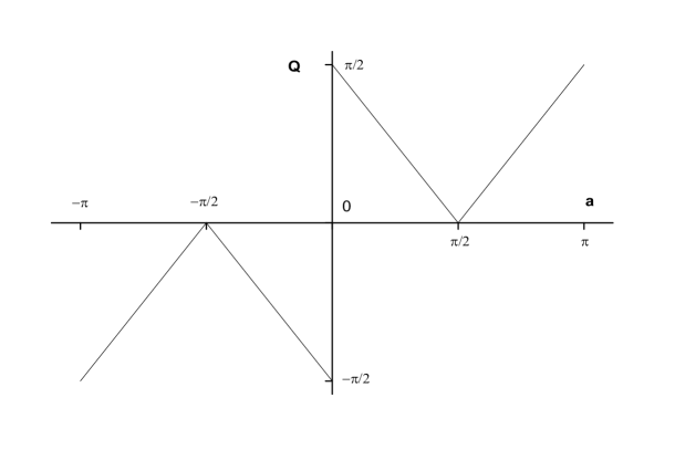
Figure 1: Soliton charge Q($a$)

As suggested by Dorey and Hollowood the charge should be defined modulo $k$ which leads to a finite spectrum depending on $k$

$$Q= \pm 1,\pm 2,...,\pm\frac{k-1}{2} \ \ \ \mbox{for}\ k\ \ \mbox{odd}\ ,$$ (12)

$$Q= \pm 1,\pm 2,...,\pm\frac{k-2}{2},\frac{k}{2} \ \ \ \mbox{for}\ k\ \ \mbox{even}\ \ .$$ (13)

From the classical expression for the charge (5) we have

$$Q=\frac{k}{\pi}(\frac{\pi}{2}-a)\ .$$ (14)

The quantisation of the charge is in fact the quantisation of $a$

$$2\pi Q=2\pi n\Leftrightarrow a=\frac{\pi}{k}\left(\frac{k}{2}-n\right)\ .$$ (15)

Through the quantisation of the charge parameter, the energy spectrum

$$M=\frac{k}{\pi}m\cos(a)\ ,$$ (16)

is also obtained

$$M(Q)=\frac{km}{\pi}\left|\ \sin\left(\frac{\pi Q}{k}\right)\right|\ .$$ (17)

The Bohr-Sommerfeld quantisation provides us only with the quantum spectrum up to leading order. According to de Vega and Maillet the next order corrections is achieved by a simple renormalisation of the coupling constant

$$\xi^{2}\rightarrow\xi_{R}^{2}=\frac{\xi^{2}}{1-\xi^{2}/4\pi}\ .$$ (18)

or equivalently

$$k\rightarrow k_{R}=k-1\ .$$ (19)

At this level an $S$-matrix may be written down that reproduces the semi-classical spectrum to leading order. In their paper Dorey and Hollowood first presented a minimal choice for the meson-soliton scattering matrix

$$S_{1Q}=F_{Q-1}(\theta)F_{Q+1}(\theta)\ .$$ (20)

which reproduced the semi-classical behaviour and agreed with the results of deVega and Maillet. Moreover, through this they confirmed that the meson in the CSG theory can be identified with the $Q=1$ soliton. The function $F_{Q}(\theta)$ is defined as

$$F_{Q}(\theta)=\frac{\sinh\left(\frac{\theta}{2}+\frac{i\pi}{2k}Q\right)}{\sinh\left(\frac{\theta}{2}-\frac{i\pi}{2k}Q\right)}\ .$$ (21)

$S$-matrices constructed from products of the $F_{Q}(\theta)$ automatically satisfy unitarity and analyticity constraints. With the above result as a starting point they proposed the following $S$-matrix for arbitrary charge

$$S_{Q_{1}Q_{2}}=F_{Q_{1}-Q_{2}}\left[\prod_{n=1}^{Q_{2}-1}F_{Q_{1}-Q_{2}+2n}\right]^{2}F_{Q_{1}+Q_{2}},$$ (22)

which satisfies all the familiar restrictions and has the correct pole structure. In addition they pointed out that this is exactly the minimal $S$-matrix associated with the Lie algebra $a_{k-1}$ and conjectured that for the specific choices of the coupling this $S$-matrix should be exact.

With the general form of the $S$-matrix the review of the bulk case is concluded. More details on the above results may be found in the relevant papers. Nevertheless, this presentation contain all the ingredients needed to examine the half-line case.

3 Semi-classical quantisation

In this section we shall attempt to build the complete spectrum of quantum boundary-bound states for the complex sine-Gordon model on a half line. The fact that the model possesses exact periodic solutions bound to the boundary makes the stationary-phase method a suitable candidate for their quantisation. The method is based on the work of Dashen, Hasslacher and Neveu [12, 13] for the semi-classical quantisation of the sine-Gordon model. In this case it appears as a generalised version of the Bohr-Sommerfeld quantisation rule

$$S_{qu}-T\frac{\partial S_{qu}}{\partial T}=2\pi n\ ,$$ (23)

where $S_{qu}=S_{cl}-\Delta$. The parameter $\Delta$ is related to the stability angles of the stationary phase approach and produces the first order quantum corrections to the classical action. We shall use the ordinary quantisation condition for the classical action $S_{cl}$ and then we shall calculate the quantum corrections factor

$$\Psi=\left(\Delta-T\frac{\partial\Delta}{\partial T}\right)\ .$$ (24)

Before embarking on quantisation, we will recall a few of the classical results about the boundary spectrum from [8]. The energy of the half-line theory is given by

$$E=\int_{-\infty}^{0}\left[\frac{|\partial_{0}u|^{2}+|\partial_{1}u|^{2}}{1-uu^{*}}+m^{2}u\right]-2C\sqrt{1-uu^{*}}$$ (25)

For a given value of $C$, the lowest energy configuration corresponds to the vacuum $u=0$. Linearising the equations of motion and the boundary conditions (2) one calculates the particle reflection coefficient can be found to be

$$K(k)=\frac{ik+C}{ik-C}$$ (26)

where $k$ is the momentum of the particle. For $C<-m$, one can show that the pole corresponds to a normalisable but in time exponentially growing perturbative mode showing that the vacuum is an unstable configuration. For $C$ in this range, the boundary can emit a real soliton which effectively swaps the sign of $C$ so that ultimately the classical field configuration returns to $u=0$, but now with $C>m$. For $|C|\leq m$, it is possible to construct a classical excited boundary state by taking $u=u_{cl}$ to be a static soliton solution of the form in (9), provided that the parameters are chosen to obey the equation

$$C=\pm\frac{m}{\sqrt{1+\tan^{2}(a)\coth^{2}(m\cos(a)x_{0})}}$$ (27)

There are other more complicated boundary states based on multi-soliton solutions such as breathers [8], but a thorough analysis of these is beyond the scope of the present study.

The boundary term of (3) preserves the $U(1)$ charge as it only depends on mod($u$). The theory remains $U(1)$ invariant and therefore the Bohr-Sommerfeld quantisation is equivalent to charge quantisation on the half line case as it was for the bulk. The quantisation condition for the classical action reads

$$S_{cl}[u_{cl}]+E_{cl}[u_{cl}]T=2\pi Q=2\pi n\ .$$ (28)

with $u_{cl}$ the static one soliton solution of (9) with parameters chosen to satisfy (27). It is a periodic solution with period $T$ exhibiting a breather-like behaviour. It provides the perfect starting point as the simplest boundary bound state of the classical theory. The position of the centre of mass will determine the charge of the bound state as a fraction of the soliton charge in the bulk. We can calculate the charge of the static soliton through the expression

$$Q=-i\int_{-\infty}^{0}dx\frac{u^{*}\partial_{0}u-u\partial_{0}u^{*}}{1-uu^{*}}\ .$$ (29)

Note that this charge is conserved without the need to add a term at the boundary. This time however the integration takes place on the half line and finally yields

$$Q=\frac{k}{2\pi}\left(\pi-b-a\right)\ .$$ (30)

The charge now depends on the boundary parameter $C=m\cos(b)$, which enters the calculation through the position of the centre of mass. As a check that this formula is correct, we can set $b=\frac{\pi}{2}$ which implies that we have the Neumann boundary condition $\partial_{x}u=0$, thus placing the soliton at exactly $x=0$. The charge is then exactly half of the equivalent charge of the soliton in the bulk (6) as expected. The quantisation condition now reads

$$Q=\frac{k}{2\pi}\left(\pi-b-a\right)=n\ ,$$ (31)

or in terms of the charge parameter

$$a=\pi-b-\frac{2\pi n}{k}\ .$$ (32)

The quantisation of $a$ provides us with the first approximation of the semi-classical spectrum

$$E_{n}=\frac{km}{2\pi}\cos(a)=\frac{km}{2\pi}\cos(\pi-b-\frac{2\pi n}{k})\ .$$ (33)

Having a general formula for the energy, it is useful to calculate the energy difference between two adjacent states. We shall use this in the following section where we shall compare it with the corresponding bootstrap result. For reasons of simplicity, we shall assume that the values of the parameters are such that the cosine is positive for both states as is their difference so that we can ignore any modulus appearing. The energy difference is then written

$$E_{n+1}-E_{n}=\frac{km}{2\pi}\left(\cos(\pi-b-\frac{2\pi(n+1)}{k})-\cos(\pi-b-\frac{2\pi n}{k})\right)\ ,$$ (34)

which after some manipulation simplifies to

$$E_{n+1}-E_{n}=\frac{km}{\pi}\cos\left(\frac{\pi}{2}-\frac{\pi}{k}\right)\cos\left(\frac{\pi(2n+1)}{k}-\frac{\pi}{2}+b)\right)\ .$$ (35)

We shall return to this result at the end of the next section, after we have obtained a relevant expression from the bootstrap programme.

Having obtained the leading order quantisation of the boundary spectrum, we calculate the first-order correction to this. The step consists of calculating the quantity $\Delta$

$$\Delta=-S_{ct}+\sum_{i=0}^{\infty}\frac{1}{2}\ \hbar\ v_{i}\ ,$$ (36)

where $v_{i}$ are the stability angles and $S_{ct}$ suitably selected counter terms to cancel any arising infinities. We shall first calculate the sum over the stability angles, while the counter terms will be introduced later. In order to obtain all possible states one has to consider the theory in a box. The theory is already bounded on the right from the original boundary, therefore another boundary should be introduced restricting the system in the finite volume $[-L,0]$. Using periodic boundary conditions will force all energy levels to become discrete. We can afterwards take the limit $L\rightarrow-\infty$ to recover the original system. The most appropriate choice would be Dirichlet boundary conditions $u=0$, which reproduce the correct behaviour of $u$ at infinity.

The stability angles are obtained by solving the linearised stability equation about a given classical solution. In our case we perturb around the static one-soliton solution. Once the solutions $\chi(x,t)$ for the stability equation are found then the stability angles can be calculated from periodicity demands

$$\chi_{i}(x,t+T)=e^{iv_{i}}\chi_{i}(x,t)\ ,$$ (37)

Instead of solving directly the stability equation we can follow the method of Corrigan and Delius to calculate the sum of the stability angles through the reflection factors. We begin with the classical two-soliton solution of the CSG model which satisfies the stability equation. By fixing the free parameters we can make one of the solitons $S_{1}$ static by taking $\delta_{1}=1$ and the other $S_{2}$ very small by taking the charge parameter $a_{2}$ close to zero. Effectively we are left with a small perturbation around a static one-soliton background. This is exactly the same method that Dashen, Hasslacher and Neveu followed to calculate the stability angles of the sine-Gordon model. At infinity the static soliton is practically zero whilst the perturbation appears as plane waves

$$\chi(x,t)=e^{-i\omega t}(e^{ik_{s}x}+R_{s}e^{-ik_{s}x})\ .$$ (38)

The reflection factor is found to be

$$R_{s}=-\frac{(\cos(b-i\theta))}{(\cos(b+i\theta))}\ \frac{(\sin(a+i\theta)-1)}{(\sin(a-i\theta)-1)}\ ,$$ (39)

where we have set $m=1$ without loss of generality. The rapidity $\theta$ which has been used is related to the momentum through $k=\sinh(\theta)$. The parameters $a$ and $b$ are the familiar charge and boundary parameters. From the above expression for $\chi(x,t)$ and (37) we can substitute

$$\Delta=\frac{1}{2}\sum_{i}v_{i}=\frac{T}{2}\sum_{i}\omega_{i}\ ,$$ (40)

where $\omega_{i}^{2}=k_{i}^{2}+1$ and the counter terms have been neglected. Placing the system in a box allows for discrete values of $k$ which should not be confused with the coupling constant. From $\Delta$ we must now subtract the vacuum contributions

$$\Delta=\frac{T}{2}\sum_{i}\sqrt{{k_{s,i}^{2}+1}}-\sqrt{k_{0,i}^{2}+1}\ .$$ (41)

From the Dirichlet boundary conditions we can obtain the following equation relating the discrete momenta with the reflection factors

$$e^{-2ik_{s}L}=\frac{(\cos(b-i\theta))}{(\cos(b+i\theta))}\ \frac{(\sin(a+i\theta)-1)}{(\sin(a-i\theta)-1)}\ .$$ (42)

A similar equation exists for the fluctuations around the vacuum

$$e^{-2ik_{0}L}=-\frac{i\sinh(\theta)+\cos(b)}{i\sinh(\theta)-\cos(b)}\ .$$ (43)

Using the same argument as Corrigan and Delius, we can define a function $\kappa(k_{0})$ such that for large $k$ we may write

$$k_{s}=k_{0}+\frac{\kappa(k_{0})}{L}\ ,$$ (44)

where the index $i$ has been suppressed. This is possible since in the limit $\theta\rightarrow+\infty$ and taking into account the general quantisation condition of (31), both reflection factors $R_{s}$ and $R_{0}$ are equal. Through the difference $k_{s}-k_{0}$ a function $\kappa(\theta)$ may be defined using the ratio of the corresponding reflection factors

$$e^{-2i\kappa(\theta)}=-\frac{(\sin(a+i\theta)-1)}{(\sin(a-i\theta)-1)}\ \frac{(\sin(b+i\theta)-1)}{(\sin(b-i\theta)+1)}\ .$$ (45)

We can now calculate $\Delta$ in terms of $\kappa$. We can substitute (44) in (41) and then expand the expression in terms of $L$. Keeping only the leading term of the expansion we end up with

$$\Delta\sim\frac{T}{2L}\sum_{i}\frac{k_{i}^{(0)}\kappa(k_{i}^{(0)})}{\sqrt{(k_{i}^{(0)})^{2}+1}}\ ,$$ (46)

which in the limit $L\rightarrow+\infty$ can be substitute with the integral form

$$\Delta=\frac{T}{2\pi}\int_{0}^{=\infty}dk\frac{k}{\sqrt{k^{2}+1}}\ \kappa(k)\ .$$ (47)

The calculation is greatly simplified if we change variables to $\theta$

$$\Delta=\frac{T}{2}\int_{0}^{+\infty}d\theta\sinh(\theta)\kappa(\theta)\ .$$ (48)

The integral is divergent but we can introduce specially chosen counter-terms to obtain a finite result. We begin with an integration by parts

$$\Delta=\frac{T}{2\pi}\left(\left[\kappa\cosh(\theta)\right]_{0}^{+\infty}-\int_{0}^{+\infty}\cosh(\theta)\frac{d\kappa}{d\theta}\right)\ .$$ (49)

The first term is not divergent since the function $\kappa$ approaches zero (through the quantisation condition) as $\theta$ goes to infinity. In this limit the combination $\kappa(\theta)\cosh(\theta)$ is zero. In addition, $\kappa(0)=0$ so the first term in (49) vanishes. The second term is however divergent and counter terms have to be introduced to cancel infinities. The latter appear in the same fashion as the logarithmic divergencies in the bulk which are tackled through normal ordering. With some straightforward manipulation the derivative term yields

$$\frac{d\kappa}{d\theta}=-{\frac{\cos(b)}{\cosh({\theta})-\sin(b)}}+{\frac{\cos(a)}{\cosh({\theta})-\sin(a)}}\ .$$ (50)

The two terms are almost identical and both divergent. A logical choice of counter-terms seems to be

$$-{\frac{\cos(b)}{\cosh(\theta)+1}}+{\frac{\cos(a)}{\cosh(\theta)+1}}\ ,$$ (51)

where the first removes the divergence associated with the boundary and the second with the one in the bulk. The complete expression to be calculated is now

$$\Delta = -\int_{0}^{+\infty}d\theta\cosh(\theta)$$

$$\left({\frac{\cos(a)}{\cosh({\theta})-\sin(a)}}-\frac{\cos(a)}{\cosh(\theta)+1}-{\frac{\cos(b)}{\cosh({\theta})-\sin(b)}}+{\frac{\cos(b)}{\cosh(\theta)+1}}\right),$$

which finally yields

$$\Delta=\frac{T}{2\pi}\left(-\cos(a)+\cos(b)+b\sin(b)+\frac{\pi}{2}\,\sin(b)-a\sin(a)-\frac{\pi}{2}\sin(a)\right)\ .$$ (52)

Having determined the form of $\Delta$ we are now in a position to calculate the corrections to the classical Bohr-Sommerfeld rule. The expression of $\Delta$ depends on the period $T$ through the charge parameter $a$

$$\sin(a)=\frac{2\pi}{T}\ .$$ (53)

The correction term of (24) is easily calculated

$$\Delta-T\frac{\partial\Delta}{\partial T}=-a-\frac{\pi}{2}\ .$$ (54)

With all the necessary parts calculated, the generalised Bohr-Sommerfeld quantisation condition finally reads

$$k_{r}(\pi-b_{r}-a)=2\pi n\ ,$$ (55)

where

$$k_{r}=k-1 b_{r}=\frac{kb-\frac{3\pi}{2}}{k-1}\ .$$ , (56)

The form of the new quantisation condition is exactly the same as the first approximation of (31), only with a redefinition for the boundary and coupling constants. The shift in the coupling constant is to be expected. In the bulk case the first order corrections amount to a simple shift in $k$ (19) as pointed by de Vega and Maillet [19]. Our result is consistent with this.

In addition to $k$, the boundary constant has to be renormalised as well. It is not clear why this renormalisation is needed or whether it should appear at all. In a paper examining the closely related $a_{k-1}$ theory, Penati and Zanon [20] argued that renormalisation of boundary parameters has to be introduced in certain models to ensure integrability at the quantum level. The renormalisation of the coupling constant and its significance remains one of the open questions for the quantum CSG theory.

4 The Bootstrap Method

In the previous section we constructed the quantum spectrum using the semi-classical stationary-phase method. Although the results are not exact, they provide us with an accurate picture of the set of states. The same spectrum can be obtained using the completely different approach of the bootstrap method. It is based on the pioneering work of Cherednik [21], Ghoshal and Zamolodchickov [9], and Fring and Köberle [22]. This way we shall be able to compare and compliment the results to acquire an even more accurate spectrum. The idea behind this method is to construct the reflection factors through the boundary bootstrap relation, and through the poles therein to identify boundary bound states. The process is analogue to the bulk case where the existence of bound states is indicated by poles found in the $S$-matrix.

Nevertheless there are quite a lot of drawbacks in this process. First of all in order to begin we need the quantum reflection factor for the particle of the theory. This cannot be obtained through any consistent procedure. Although the principles of analyticity, unitarity and crossing symmetry along with the boundary Yang-Baxter equation restrict the form of the reflection factor enough, it is impossible to pin it down completely. It is therefore a matter of “selecting” the correct reflection factor which should satisfy all constraints whilst introducing a pole corresponding to a boundary bound state.

After carefully deciding on the correct reflection factor for the particle, we are faced with a second problem. Although we are only concerned with poles in the reflection factor which appear on the physical strip (which in the half line case is $\Im(\theta)\ \epsilon\ [0,\pi/2]$), not all of them correspond to boundary bound states. It is quite difficult to explain the appearance of all the poles which lie within the physical strip and no work until now exists to offer a systematic treatment of poles encountered.

Another difficult arises with the determination of the CDD factors in the reflection matrix. The restrictions imposed on the reflection factor may determine it up to a set of factors, quite like the CDD factors of the $S$-matrix. However the reflection CDD factors which are also restricted by the same constraints, introduce more poles which are also difficult to explain.

Considering all the above we shall attempt to construct the quantum boundary-bound state spectrum for the CSG theory but our study will be superficial. It is not our objective to fully explain the quantum structure of the model but rather to verify crudely our semi-classical results. The detailed explanation of poles in the reflection factors, the determination of a general form for the reflection CDD factors and the comparison of the results with similar theories are quite fascinating problems but are beyond the scope of this paper. In the following section we shall present a suitable form for the quantum reflection factor for the particle of the CSG model.

4.1 Quantum reflection factor for the CSG particle

We begin our attempt to introduce a suitable reflection matrix $K_{1}$ for the CSG particle with the assumption that it should be made out of $F$ factors that were defined in (21). It is a natural selection as both the boundary Yang-Baxter equation and the bootstrap equations relate reflection matrices with the $S$-matrix which is expressed only in terms of such functions. There is another advantage to this choice. Unitarity, real analyticity and $2\pi i$-periodicity requirements are automatically satisfied if $K$ appears as a product of such factors. Some of the most important properties enjoyed by these functions include the following

$$F_{Q}(\theta)F_{Q}(-\theta)=1\ , \ F_{2Q}(2\theta)=-F_{Q}(\theta)F_{Q+k}(\theta)\ , \ F_{Q}(\theta+i\pi)=-F_{Q+k}(\theta)\ .$$

The first of the above is responsible for the fulfillment of the unitarity requirement. The remaining demonstrate basic transformations between rapidity and charge and will be used in the bootstrap and crossing symmetry equations.

It should be noted that since there is no degeneracy in the spectrum we expect $K$ to be diagonal. This, in conjunction with a diagonal $S$-matrix, renders the boundary Yang-Baxter equation

$$K_{a}(\theta_{a})S_{ab}(\theta_{a}+\theta_{b})K_{b}(\theta_{b})S_{ab}(\theta_{a}-\theta_{b})=S_{ab}(\theta_{a}-\theta_{b})K_{b}(\theta_{b})S_{ab}(\theta_{a}+\theta_{b})K_{a}(\theta_{a})\ ,$$

trivial. In their paper Dorey and Hollowood identified the CSG particle with the $Q=1$ soliton. In this context the first real constraint for $K$ comes from the crossing symmetry relation which for our case is written as

$$K_{1}(\theta)K_{\bar{1}}(\theta+i\pi)=S_{1,1}(2\theta)\ ,$$ (57)

where $K_{\bar{1}}$ is the reflection of the antiparticle and $S_{1,1}$ is the two particle scattering matrix. Dorey and Hollowood noted that the CSG $S$-matrix is identical to the minimal $a_{k-1}$ $S$-matrix which in turn can be recovered from the $a_{k-1}^{(1)}$ Affine Toda field theory (ATFT) when the parts involving the coupling constant are omitted. It is therefore reasonable to build our reflection matrix based on the proposed form for the particle reflection matrix of the boundary $a_{k-1}^{(1)}$ ATFT theory. In their paper Delius and Gandenberger [23] present a general form for the particle reflection matrix of the $a_{k-1}^{(1)}$ ATFT. As in the $S$-matrix case the reflection matrix is a product of two parts, out of which only one depends on the coupling constant. Each part satisfies the bootstrap independently so we can recover a $K$-matrix for our model by simply ignoring the coupling dependent pieces. The block notation implies $(x)=F_{x}(\theta)$ and shall be used henceforth in parallel with $F$. Ignoring the parts involving the coupling constant, the remaining factors

$$K_{n}=\sum_{c=1}^{n}(c-1)(c-k) n=1..(k-1)\ ,$$ , (58)

constitute a complete set satisfying the crossing-symmetry condition (57) as well as the reflection bootstrap equation

$$K_{c}(\theta_{c})=K_{a}(\theta_{a})K_{b}(\theta_{b})S_{ab}(\theta_{a}+\theta_{b})\ .$$ (59)

This is not unexpected as both theories share the same minimal $S$-matrix . This however creates a problem as $K$ does not contain any poles which can be related to boundary-bound states. This means that should any additional factors be added by hand to introduce the required poles, they should be added in such a way that they cancel between them in the crossing and bootstrap relations. This in turn suggests that the new factors are nothing more than CDD factors for the reflection matrix. Placing the poles in the CDD factors simplifies the whole procedure of determining a suitable particle reflection matrix since they satisfy simpler relations.

Real analyticity and unitarity conditions once again prompt us to construct our CDD factors out of block functions, so that the former are satisfied automatically. In order for the crossing relation to be satisfied any block factor $(x)$ should be accompanied by the charge conjugate factor $(k-x)$. Delius and Gandenberger showed for such a combination the bootstrap closes.

Now that we have a consistent way of adding factors we need to find where the poles should appear. We begin with the simple formation of the boundary bound state described in (Fig. 2). During the process both energy and charge are conserved. We begin with the charge conservation. Far away from the boundary the soliton (particle) behaves as in the theory in the bulk. Its’ charge is equal to the normal soliton charge $Q_{1}=\frac{k}{\pi}(\frac{\pi}{2}-a_{1})$. After the formation of the bound state the charge $Q_{2}$ is given by the formula (30). Equating these yields

$$(\frac{\pi}{2}-a_{1})=\frac{1}{2}({\pi}-b-a_{2})\ .$$ (60)

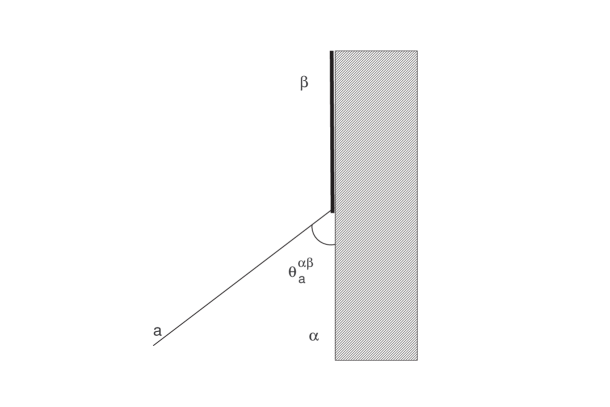
Figure 2: The boundary bound state

Using the same arguments we can write down an equation describing the conservation of energy

$$4m\cos(a_{1})\cosh(\theta)-2m\cos(b)=2m\cos(a_{2})\ ,$$ (61)

where the $-2m\cos(b)$ term is the boundary energy contribution when the field is zero. From (60) and (61) we can determine the rapidity $\theta$ at which the boundary bound state is formed

$$\theta_{n}^{(0,n)}=i\frac{\pi}{k}\left(n+B\right) B=\frac{k}{\pi}\ b-\frac{k}{2}\ .$$ where (62)

For the above relation the quantisation condition of (31) was also used. Now that we have determined where the pole should be, we need to express it in block notation. It is easy to see that since $(x)$ has a pole in the denominator at $\theta=i\frac{\pi}{k}x$, we therefore need a block $(n+B)$ and its counterpart $(k-n-B)$ for the CDD factor of $K_{n}$.

Nevertheless the blocks containing the pole should not be the only components of the CDD factor. On the contrary we expect the number of CDD factors in $K_{n}$ to increase as $n$ increases towards $\frac{k}{2}$ and then to decrease as it approaches $k-1$. Since we have $k-1$ particles and the theory is $Z_{k}$ symmetric we expect $K_{k+1}=K_{1}$. Moreover since the reflection matrix remains the same under charge conjugation we expect $K_{n}=K_{k-n}$.

Although it is not easy to derive the general formula for the CDD factors in the $K_{n}$ reflection matrix, we can decide on a minimal choice for $K_{1}$. We opt for a CDD factor containing only the first pole and its’ charge conjugate counterpart. The full reflection factor then reads

$$K_{1}^{(0)}=(1+B)(k-1-B)(1-k)\ .$$ (63)

The superscript denotes the boundary excitation state. In this particular case $K_{1}^{(0)}$ describes the reflection of a soliton of charge $Q=1$ from an unexcited boundary. We ignore the poles coming from the non-CDD part of $K_{1}^{(0)}$. We shall address this issue at the closing stages of this section. The pole associated with the $(1+B)$ factor corresponds to the lowest boundary bound state with energy

$$E_{b}^{(1)}=\frac{km}{2\pi}\cos(\pi-b-\frac{2\pi}{k})\ .$$ (64)

which is formed when a soliton of charge $Q=1$ (which is the particle of the theory) fuses with the boundary. The conjugate term $(k-1-B)$ also has a pole but does not lie within the physical strip $\Im(\theta)\ \epsilon\ (0,\frac{\pi}{2})$. Note that in the classical limit $k\rightarrow\infty$ the reflection factor

$$K_{1}^{(0)}\rightarrow\frac{i\sinh(\theta)+\cos(b)}{i\sinh(\theta)-\cos(b)}$$ (65)

in agreement with the identification of the charge $1$ soliton as a particle and the classical particle reflection factor (26).

With $K_{1}^{(0)}$ as a starting point we can construct the whole set of $K_{n}^{(0)}$ factors by using the reflection bootstrap (59). In addition, we can apply the boundary bootstrap

$$K_{b}^{(\beta)}=S_{ab}(\theta_{b}-\theta_{a}^{\alpha\beta})K_{b}^{(\alpha)}S_{ab}(\theta_{b}+\theta_{a}^{\alpha\beta})\ ,$$ (66)

to each of them to obtain the corresponding reflection matrices from the excited boundary. In both cases new block factors are generated carrying poles which indicate new bound states. If our choice for the CDD factor in (63) is correct we expect the bootstrap to close, i.e. to end up with a finite spectrum of states which is repeated after $k$ steps. Pictorially this can be seen in (Fig. 3)

Figure 3: The Bootstrap Programme

As a starting point we can calculated the reflection factor of a charge $Q=2$ soliton bouncing off the unexcited boundary

$$K_{2}^{(0)}(\theta)=K_{1}^{(0)}(\theta-\frac{i\pi}{k})K_{1}^{(0)}(\theta+\frac{i\pi}{k})S_{1,1}(2\theta).$$ (67)

Substituting $K_{1}^{(0)}$ from (63) and $S_{1,1}$ from (22) we finally get

$$K_{2}^{(0)}=(2+B)(k-2-B)(B)(k-B)(1-k)(1)(2-k)\ .$$ (68)

This result confirms that the general formula of (58) forms a complete set. Henceforth we shall ignore the basic blocks of the reflection matrix as they are a consistent set and concentrate only on the CDD factors which carry all necessary information about boundary bound states. The first four terms are the CDD factor for $K_{2}^{(0)}$ which introduce two new poles. An equally straightforward calculation is that of $K_{4}^{(0)}$ which is found to be

$$K_{4}^{(0)}=\frac{(B+4)(B+2)(k-B+4)(k-B+2)}{(-B)(-B+2)(-k+B+2)(-k+B+4)}\ .$$ (69)

A pattern begins to emerge from these simple results. The CDD factor of $K_{n}^{(0)}$ always involves the block pair $(n+B)(k-n-B)$. This is the first consistent appearance of poles in the reflection matrices. This is also the complete set of poles that are produced by the bootstrap programme. With an arbitrary coupling constant $k$, it is not easy to demonstrate the complete mechanism of pole production. This can easily be seen by fixing $k$ to an integer value. One can then see the whole range of poles produced and how the bootstrap miraculously closes.

4.2 The boundary bootstrap

In the previous section we proposed a suitable expression for the $K_{1}^{(0)}$ reflection factor and saw how through the reflection bootstrap all the $K_{n}^{(0)}$ factors can be obtained. We now turn to the boundary bootstrap to construct the boundary reflection factors of solitons bouncing off an excited boundary. We shall only examine the boundary bootstrap for the particle reflection factor. Through the reflection bootstrap all other states can be built (Fig. 3). Once again we are facing the problem that with $k$ arbitrary and a charge-varying $S$-matrix we are not in a position to identify all poles or cancel terms in the reflection matrix. We therefore shall attempt to find a general formula for the energy difference between adjacent boundary bound states. This should be enough to build the whole spectrum of states beginning with the energy of the first bound state.

We begin with the boundary bootstrap equation (66) for $K_{1}^{(1)}$ which is

$$K_{1}^{(1)}=K_{1}^{(0)}S_{1,1}(\theta+\theta_{1}^{(0,1)})S_{1,1}(\theta-\theta_{1}^{(0,1)})\ ,$$ (70)

where $\theta_{1}^{(0,1)}=i\frac{\pi}{k}\left(1+B\right)$ denotes the pole in $K_{1}^{(0)}$. The product of $S$-matrices in the above relation is equal to a shift in their charge. In general the following relation holds for any $\psi$.

$$S_{1,1}(\theta+i\psi)S_{1,1}(\theta-i\psi)=(2+\frac{k}{\pi}\psi)(2-\frac{k}{\pi}\psi)\ .$$ (71)

Putting everything together yields

$$K_{1}^{(1)}=(1+B)(k-1-B)(3+B)(1-B)\ .$$ (72)

Once again we have only used the CDD factors and ignored terms not involving the boundary constant. We see through this procedure a new pole appears from the block $(3+B)$ corresponding to the absorption of a charge $Q=1$ particle into the charge $Q_{b}=1$ boundary. This will be used as an input to find a new pole in $K_{1}^{(2)}$

$$K_{1}^{(2)}=(k-1-B)(3+B)(1-B)(5+B)\ ,$$ (73)

where a cancellation has already taken place. The new pole comes from the block factor $(5+B)$ which will be used in the next step. The expression for $K_{1}^{(3)}$ is

$$K_{1}^{(3)}=(k-1-B)(1-B)(5+B)(7+B)\ ,$$ (74)

where new factor $(-3-B)$ has cancelled with the block factor $(3+B)$ and the factor $(7+B)$ has introduced a new pole. This procedure will not continue indefinitely. After $k$ steps we expect to return to original form of $K_{1}^{(0)}$. However it is clear that the $K_{1}^{(n)}$ reflection matrix will have a pole indicated by the block factor $(2n+1+B)$ at $\psi_{n}=\frac{\pi}{k}(2n+1+B)$. Having a general formula about the $n$-th pole allows us to write down a recursive relation for the energies of the bound states. We begin with the energy of the first bound state. The difference between the first excited boundary state and the non-excited boundary is

$$E_{1}-E_{0}=A\cos(\psi_{0})\ .$$ (75)

The right hand side is equal to the mass of the incoming particle that binds with the boundary at a fixed angle $\theta=i\psi_{0}$. The parameter A is related to the mass of the particle and will be determined from the comparison with the semi-classical results. The formula may be used recursively to finally yield

$$E_{n+1}-E_{n}=A\cos(\psi_{n})=A\cos(\frac{\pi}{k}(2n+1+B))\ .$$ (76)

This formula should be compared with the one derived from the semi-classical approach (35). Both describe the exact same energy gaps between two bound states. The arbitrary parameter $A$ in (76) can be read directly from (35)

$$A=\frac{km}{\pi}\cos\left(\frac{\pi}{2}-\frac{\pi}{k}\right)=\frac{km}{\pi}\sin\left(\frac{\pi}{k}\right)$$ (77)

which is equal to the energy of the particle. In the limit that $k\rightarrow\infty$ (the classical limit) the soliton becomes infinitesimally small and the boundary-bound states spectrum become continuous.

We conclude this section with a brief discussion about the poles appearing in the reflection matrix. We expect the non-CDD poles in (58) to be explained in terms of a on-shell triangle diagram as is the case for the $a_{n}^{(1)}$ affine Toda theory. A full discussion can be found in [23]. The remaining poles appear in the CDD factors and are the ones associated with the boundary-bound states. The full set of poles generated from the bootstrap programme come from the general blocks $(n+B)$ and $(k-n-B)$ which have poles at

$$\psi_{n}=\frac{\pi}{k}n-\frac{\pi}{2}+b \psi_{n}^{\prime}=\pi-\left(\frac{\pi}{k}n-\frac{\pi}{2}+b\right)$$ and (78)

From the forms above we can see that if $\theta_{n}$ lies in the physical strip $(0,\frac{\pi}{2})$ then $\theta_{n}^{\prime}$ does not, and vice versa. Assuming that the pole is at $\theta_{n}$ then it lies in the physical strip if

$$\frac{\pi}{2}>\psi_{n}>0 \Leftrightarrow 1>\frac{n}{k}+\frac{b}{\pi}>\frac{1}{2}$$ (79)

As soon the above condition is no longer true then the pole appears in the conjugate block at $\psi_{n}^{\prime}$. This however does not alter any of our results. From (76) we can see that $\psi_{n}$ or $\psi_{n}^{\prime}$ appear in the argument of the cosine so both correspond to the same absolute energy difference between two states.

5 Discussion

We used semi-classical method to obtain the boundary spectrum of the CSG model. Having incorporated the unitary and crossing constraints, we found that we needed to adjust our simplest guess for the reflection factor of a particle off an unexcited boundary by a CDD factor, in order that the reflection factor in question exhibited a pole corresponding to the lowest bound state of the boundary. Reflection factors for higher charge solitons, and for particles and solitons scattering off excited boundaries were obtained by iterating the reflection bootstrap and boundary bootstrap respectively. The rest of the excited boundary spectrum could be deduced by analysing the poles in these higher reflection factors, and, perhaps remarkably, it coincides with that obtained by semi-classical methods. The reflection and boundary bootstrap both close because the minimal choice for $K_{n}$ (58) is consistent with our $S$-matrix and because the introduced blocks are CDD factors.

One final point to be made is that although we have used for our comparison equations (31) and (35) which correspond to the first approximation in the semi-classical approach, we can extend our results to agree with the first order corrections by simply substituting everywhere $k=k_{r}$ and $b=b_{r}$. The redefinition of both parameters change nothing in the bootstrap approach. If we believe, as seems to be the case for the bulk coupling constant, that the boundary coupling constant receives no further corrections at higher orders in perturbation theory, then the formulae containing $k_{r}$ and $b_{r}$ would be exact.

References

- [1] Fernando Lund and Tullio Regge. Unified approach to strings and vortices with soliton solutions. Phys. Rev., D14:1524, 1976.
- [2] K. Pohlmeyer. Integrable hamiltonian systems and interactions through quadratic constraints. Commun. Math. Phys., 46:207, 1976.
- [3] Carlos R. Fernandez-Pousa, Manuel V. Gallas, Timothy J. Hollowood, and J. Luis Miramontes. The symmetric space and homogeneous sine-gordon theories. Nucl. Phys., B484:609–630, 1997.
- [4] Carlos R. Fernandez-Pousa and J. Luis Miramontes. Semi-classical spectrum of the homogeneous sine-gordon theories. Nucl. Phys., B518:745–769, 1998.
- [5] O. A. Castro-Alvaredo, A. Fring, C. Korff, and J. L. Miramontes. Thermodynamic bethe ansatz of the homogeneous sine-gordon models. Nucl. Phys., B575:535–560, 2000.
- [6] P. Dorey and J. L. Miramontes, Mass scales and crossover phenomena in the homogeneous sine-Gordon models Nucl. Phys. B697: 405-461,2004.
- [7] B. S. Getmanov. New lorentz invariant systems with exact multi - soliton solutions. (in russian). Pisma Zh. Eksp. Teor. Fiz., 25:132–136, 1977.
- [8] Peter Bowcock and Georgios Tzamtzis. The complex sine-Gordon model on a half-line hep-th/0203139
- [9] Subir Ghoshal and Alexander B. Zamolodchikov. Boundary s matrix and boundary state in two-dimensional integrable quantum field theory. Int. J. Mod. Phys., A9:3841–3886, 1994.
- [10] H. J. de Vega and J. M. Maillet. Renormalization character and quantum s matrix for a classically integrable theory. Phys. Lett., B101:302, 1981.
- [11] H. J. de Vega and J. M. Maillet. Semiclassical quantization of the complex sine-gordon field theory. Phys. Rev., D28:1441, 1983.
- [12] Roger F. Dashen, Brosl Hasslacher, and Andre Neveu. The particle spectrum in model field theories from semiclassical functional integral techniques. Phys. Rev., D11:3424, 1975.
- [13] Roger F. Dashen, Brosl Hasslacher, and Andre Neveu. Nonperturbative methods and extended hadron models in field theory. 1. semiclassical functional methods. Phys. Rev., D10:4114, 1974.
- [14] Guy Bonneau. Renormalizability and nonproduction in complex sine-gordon model. Phys. Lett., B133:341, 1983.
- [15] Nicholas Dorey and Timothy J. Hollowood. Quantum scattering of charged solitons in the complex sine- gordon model. Nucl. Phys., B440:215–236, 1995.
- [16] Ioannis Bakas. Conservation laws and geometry of perturbed coset models. Int. J. Mod. Phys., A9:3443–3472, 1994.
- [17] Ivan Ventura and Gil C. Marques. The bohr-sommerfeld quantization rule and charge quantization in field theory. Phys. Lett., B64:43, 1976.
- [18] C. Montonen. On solitons with an abelian charge in scalar field theories. 1. classical theory and bohr-sommerfeld quantization. Nucl. Phys., B112:349, 1976.
- [19] H. J. de Vega, J. Ramirez Mittelbrunn, M. Ramon Medrano, and N. Sanchez. The general solution of the 2-d sigma model stringy black hole and the massless complex sine-gordon model. Phys. Lett., B323:133–138, 1994.
- [20] S. Penati and D. Zanon. Quantum integrability in two-dimensional systems with boundary. Phys. Lett., B358:63–72, 1995.
- [21] I. V. Cherednik. Factorizing particles on a half line and root systems. Theor. Math. Phys., 61:977–983, 1984.
- [22] Andreas Fring and Roland Koberle. Factorized scattering in the presence of reflecting boundaries. Nucl. Phys., B421:159–172, 1994.
- [23] Gustav W. Delius and Georg M. Gandenberger. Particle reflection amplitudes in a(n)(1) toda field theories. Nucl. Phys., B554:325–364, 1999.
- [24] E. Corrigan and G. W. Delius, Boundary breathers in the sinh-Gordon model J. Phys. A 32 (1999) 8601.