hep-th/0612116

Cosmological unification
of string theories

Simeon Hellerman and Ian Swanson

School of Natural Sciences, Institute for Advanced Study
Princeton, NJ 08540, USA

Abstract

We present an exact solution of superstring theory that interpolates in time between an initial type 0 phase and a final phase whose physics is exactly that of the bosonic string. The initial theory is deformed by closed-string tachyon condensation along a lightlike direction. In the limit of large tachyon vev, the worldsheet conformal field theory precisely realizes the Berkovits-Vafa embedding of bosonic string theory into superstring theory. Our solution therefore connects the bosonic string dynamically with the superstring, settling a longstanding question about the relationship between the two theories.

December 13, 2006

1 Introduction

We recently presented several exact classical solutions of string theory in diverse dimensions, describing bulk closed-string tachyon condensation along a lightlike direction [1, 2]. The solutions of [1] describe “bubbles of nothing” nucleating in unstable backgrounds, and Ref. [2] focuses on dynamical transitions from unstable linear dilaton backgrounds to string theories in lower numbers of dimensions. In the latter case, the initial linear-dilaton theories include bosonic, type 0 and unstable heterotic string theories. They relax into final-state theories that can exist in a wide range of spacetime dimensions including critical, supercritical, and subcritical cases down to $2D$. In all examples, however, the basic kind of string theory is unchanged between the initial and final configurations. That is, the transitions in [2] connect bosonic string theories to other bosonic string theories, heterotic string theories to one another, and type 0 theories to other type 0 or type II string theories, the two differing only in their GSO projection.

In this paper we study a related model of lightlike tachyon condensation in type 0 string theory, where the tachyon again depends only on $X^{+}$, and is independent of the $D-2$ dimensions transverse to $X^{\pm}$. In this example, the effect of the tachyon condensate is not to change the number of spacetime dimensions but to change the kind of string theory altogether. Deep inside the region of nonzero tachyon condensate, at $X^{0}\to+\infty$, the string propagates freely without a potential, but the worldsheet supersymmetry is broken spontaneously. The result is that the effective worldsheet gauge symmetry and constraint algebra are described by the ordinary Virasoro algebra rather than its super-Virasoro extension, and the physical state space is described by the Hilbert space of a bosonic string rather than that of a superstring.

It turns out that our solution precisely realizes an old mechanism [3] by which bosonic string theory can be embedded in the solution space of the superstring. Since worldsheet supersymmetry is a gauge artifact, this mechanism is perfectly consistent. We note that the model in [3] is itself a specific instance of a very general idea, namely the completely nonlinear realization of supersymmetry [4]. The additional input of [3] is essentially conformal invariance and coupling to two-dimensional gravity.

The meaning of the embedding of [3] has remained obscure. One might have interpreted the bosonic string as merely a formal solution to the equations of superstring theory, disconnected from the more familiar solution space. We are led to ask: Is bosonic string theory accessible dynamically from a conventional state of superstring theory?

We settle this question in the affirmative. In the case we study here, the embedding of [3] describes only the $X^{+}\to+\infty$ limit of the theory (which we refer to as the infrared limit). The $X^{+}\to-\infty$ (or ultraviolet) limit is described by a type 0 superstring, with worldsheet supersymmetry linearly realized on free fields in the conventional way. At finite $X^{+}$, the system is a deformation interpolating between the two. Our solution therefore represents a dynamical transition between the type 0 superstring and the bosonic string.

Key to the analysis is the fact that the solutions we consider have no dynamical quantum corrections. This can be seen at the level of Feynman diagrams. Our worldsheet theory is a theory of free massless scalar fields, perturbed by an interaction term depending only on $X^{+}$ and its superpartners $\psi^{+},~{}\tilde{\psi}^{+}$. Worldsheet propagators are oriented, pointing from fields in the $X^{+}$ multiplet to the $X^{-}$ multiplet. Since interaction vertices have only outgoing lines, connected Feynman diagrams have at most one interaction vertex (similar considerations were employed in [1, 2]).

It follows that connected correlators of fields in the $X^{+}=-\infty$ limit have no loop corrections, and they can receive contributions from at most one tree graph. Even then, all operators in the expectation value must be in the multiplet of $X^{-}$, with no $X^{+}$ multiplet degrees of freedom. By the same diagrammatic argument, connected interaction contributions to operator product expansions can have only $X^{-}$ multiplets on the left-hand side and only $X^{+}$ multiplets on the right-hand side. We exploit these properties to understand the large-$X^{+}$ behavior of the theory by solving the OPE altogether.

In the next section we discuss tachyon condensation in the type 0 theory. We find a solution, exact in ${\alpha^{\prime}}{}$, in which the tachyon increases exponentially along the lightlike direction $X^{+}$. The $2D$ CFT has a large interaction term in the limit $X^{+}\to+\infty$, so we choose a dual set of variables whose interactions are suppressed, rather than enhanced, in the limit of large $X^{+}$. To gain an understanding of the basic physics, we perform the change of variables classically, ignoring singularities in products of local operators. In Section 4 we work out operator ordering prescriptions and derive the transformation on the supercurrent and stress tensor at the quantum level. In Section 5 we perform additional transformations to make manifest the $(D-1)$-dimensional Poincaré invariance of the $X^{+}\to+\infty$ limit. Rewriting the stress tensor and supercurrent in an $SO(D-1)$-symmetric form, we see that the large-$X^{+}$ limit of our theory is exactly described by a $(1,1)$ superconformal field theory [3], wherein the worldsheet supersymmetry is completely nonlinearly realized. In Section 6 we discuss the physics of the $X^{+}\to+\infty$ limit, and we present general conclusions in Section 7. Various technical issues are addressed in the appendices, including the presentation of specific canonical transformations, the direct computation of OPEs, the computation of the BRST cohomology in the Berkovits-Vafa formalism, and a description of the Ramond sectors in this theory.

2 Lightlike tachyon condensation in type 0 string theory

We begin by considering type 0 strings propagating in a timelike linear dilaton background in $D$ dimensions $X^{M}$, which has $G_{MN}=\eta_{MN}$ and $\Phi\equiv V_{M}X^{M}$, with $V_{M}$ constant. This background describes a cosmological background of type 0 string theory. The cosmology is an expanding Friedman-Robertson-Walker solution with flat spatial sections. Its stress-energy comes from the dynamics of the dilaton field $\Phi$, whose potential gives rise to a quintessent cosmology with equation of state

$$w\equiv{p\over\rho}=-{{D-3}\over{D-1}}\ .$$ (2.1)

This value of $w$ is exactly on the boundary between equations of state that give rise to accelerating and decelerating behavior for the scale factor [1]. Canonically normalized fluctuations of the metric and dilaton have exponentially growing modes, but these do not represent true instabilities. Their growth is always compensated by the exponentially decreasing string coupling, so their coupling to a mode of the string at most stays constant with time, and in general decreases [1, 5]. The same is true of excited, massive modes of the string. No massless or massive field ever represents a true instability.

Only tachyons, the lowest modes of the string, can grow fast enough with time to overcompensate their decreasing coupling to the string worldsheet. In [1, 2] we examined certain exact solutions in which the tachyon has a nonzero value. These solutions represent bubbles of nothing, and dynamical transitions to string theories with lower numbers of dimensions. In this paper we will examine a third type of exact solution with nonzero tachyon.

Our starting point is the Lagrangian for a timelike linear dilaton theory on a flat worldsheet, describing $D$ free massless fields and their superpartners:

$${\cal L}_{\rm kin}={\frac{1}{2\pi}}G_{MN}\left[\,{\frac{2}{{{\alpha^{\prime}}{}}}}(\partial_{+}X^{M})(\partial_{-}X^{N})-i\psi^{M}(\partial_{-}\psi^{N})-i\tilde{\psi}^{M}(\partial_{+}\tilde{\psi}^{N})\,\right]\ .$$ (2.2)

On a curved worldsheet, the dilaton couples to the worldsheet Ricci scalar:

$$\Delta{\cal L}={1\over{4\pi}}\,\Phi(X)~{}{\cal R}_{\rm worldsheet}\ .$$ (2.3)

The magnitude of the dilaton gradient $V_{M}$ must satisfy $4{\alpha^{\prime}}{}V^{2}=-(D-10)$, so we take

$$V_{+} = V_{-}=-{{q}\over{\sqrt{2}}}\ ,$$

$$\,\,V_{i} = 0,\qquad i=2,\cdots,D-1\ ,$$

$$q \equiv \sqrt{{D-10}\over{4{\alpha^{\prime}}{}}}\ ,$$ (2.4)

assuming the dilaton rolls to weak coupling in the future. The $\pm$ labels above refer to the light-cone directions $X^{\pm}\equiv{1\over{\sqrt{2}}}\left(\,X^{0}\pm X^{1}\,\right)$. In addition to the massless modes of the metric $G_{MN}$, NS B-field $B_{MN}$ and dilaton $\Phi$, there is also a tachyon ${\cal T}$ with mass-squared $m^{2}=-{2\over{{\alpha^{\prime}}{}}}$. Here and throughout the paper, we are using the terms massive, massless, tachyonic, mass-squared, etc. in the sense described (for NS fields) in [1].

We would like to consider solutions for which the type 0 tachyon condenses, growing exponentially in the lightlike direction $X^{+}$. That is, we make the ansatz

$${\cal T}\equiv\tilde{\mu}\,{\rm exp}\left(\beta X^{+}\right)\ .$$ (2.5)

The linearized equation of motion for the tachyon is

$$\partial^{2}{\cal T}-2V\cdot\partial{\cal T}+{2\over{\alpha^{\prime}}{}}{\cal T}=0\ ,$$ (2.6)

which fixes

$$\beta q={{\sqrt{2}}\over{\alpha^{\prime}}{}}\ .$$ (2.7)

The type 0 tachyon couples to the worldsheet as a $(1,1)$ superpotential:

$${\cal L}_{\rm int}={i\over{2\pi}}\,\int d\theta_{+}d\theta_{-}\,{\cal T}(X)\ ,$$ (2.8)

which gives rise to a potential and Yukawa term

$${\cal L}_{\rm int}=-{{{\alpha^{\prime}}{}}\over{16\pi}}G^{MN}\,\partial_{M}{\cal T}\partial_{N}{\cal T}+{{i{\alpha^{\prime}}{}}\over{4\pi}}\partial_{M}\partial_{N}{\cal T}\,\tilde{\psi}^{M}\psi^{N}\ ,$$ (2.9)

as well as a modified supersymmetry transformation for the fermions:

$$\{Q_{-},\psi^{M}\} = -\{Q_{+},\tilde{\psi}^{M}\}=F^{M}\ ,$$

$$F^{M} \equiv -\,\sqrt{{{\alpha^{\prime}}{}}\over 8}\,G^{MN}\partial_{N}{{\cal T}}\ .$$ (2.10)

Since the gradient of the tachyon is null, the worldsheet potential ${{{\alpha^{\prime}}{}}\over{16\pi}}G^{MN}\,\partial_{M}{\cal T}\partial_{N}{\cal T}$ is identically zero. There is nonetheless a nonvanishing $F$-term and a Yukawa coupling between the lightlike fermions:

$$F^{-} = +{{q\sqrt{{\alpha^{\prime}}{}}\mu}\over 2}\,{\rm exp}\left(\beta X^{+}\right)\ ,$$

$${\cal L}_{\rm Yukawa} = {{i\,\mu}\over{4\pi}}\,{\rm exp}\left(\beta X^{+}\right)\tilde{\psi}^{+}\psi^{+}\ ,$$ (2.11)

where $\mu\equiv\beta^{2}{\alpha^{\prime}}{}\,\tilde{\mu}$.

Our goal is to determine the $X^{+}\to\infty$ limit of this theory. Since there is no worldsheet potential, in contrast to the cases studied in [1, 2], no string states are expelled from the interior of the bubble. Instead, all states are permitted within the bubble: To describe the late-time behavior of this system we must understand the dynamics of states in the ${\cal T}\neq 0$ region.

The physics of the $X^{+}\to\infty$ phase may seem counterintuitive. The nonvanishing $F$-term signals spontaneously broken worldsheet supersymmetry, but the vacuum energy vanishes. This is not a contradiction, as the worldsheet supersymmetry is realized nonunitarily when treated as a global symmetry. If the supersymmetry is thought of as local, there is again no contradiction because there are no generators of the superalgebra that act on the physical-state Hilbert space. From the latter point of view, the vanishing of the vacuum energy in a theory with spontaneously broken local supersymmetry is very much like the physics of the so-called ‘no-scale’ vacua of $D=4,~{}{\cal N}=1$ supergravity.

This analogy lends a clue as to what the physics in the $X^{+}\to+\infty$ limit might be, where the $F$ term becomes infinite in size. Consider a no-scale vacuum of ${\cal N}=1$ supersymmetry in four dimensions, in the limit where the $F$-term becomes large and the vacuum energy is fine-tuned to zero. If one holds fixed the relevant parameters of the theory other than the gravitino mass $m_{3/2}$, the gravitino becomes infinitely massive and decouples. In this limit one can introduce arbitrary small deformations to the Lagrangian, including independent variations of the masses of bose and fermi fields that would otherwise lie in degenerate multiplets. In other words, the system has a non-supersymmetric Minkowski vacuum that harbors no trace of the local supersymmetry of the finite-$m_{3/2}$ theory.

The $2D$ worldsheet CFT in our system behaves analogously: the $X^{+}\to\infty$ limit exhibits none of the local worldsheet supersymmetry of the $X^{+}\to-\infty$ theory. It is important to note that the worldsheet supersymmetry is still formally present, even at infinitely large $X^{+}$. In this limit, however, the supersymmetry is vacuous, insofar as its role is simply to eliminate the conformal goldstino degrees of freedom. The system therefore becomes precisely equivalent to a bosonic string theory.

As noted above (and to be demonstrated explicitly below), the $X^{+}\to\infty$ limit of our solution is a dynamical realization of the Berkovits-Vafa embedding of the bosonic string into the space of solutions of superstring theory [3]. We will thus describe this limit of our model in exactly the language and notation of [3]. In particular, we will connect our model to that of [3] by performing a series of canonical transformations on the worldsheet fields. In the next section we describe in detail the first stage of these manipulations.

3 From ultraviolet to infrared variables

We define the indices $\mu,\nu,\cdots$ to run only over the light-cone coordinates $\{+,-\}$, and denote the $D-2$ directions transverse to the light-cone directions by $i,j,\ldots\,$ Using the canonical flat metric $G_{+-}=G_{-+}=-1$, our Lagrangian for the light-cone multiplets $X^{\mu},~{}\psi^{\mu},~{}\tilde{\psi}^{\mu}$ is:

$${\cal L}_{\rm LC} = {i\over{\pi}}\tilde{\psi}^{+}\partial_{+}\tilde{\psi}^{-}+{i\over{\pi}}\psi^{+}\partial_{-}\psi^{-}+{{iM}\over{2\pi}}\tilde{\psi}^{+}\psi^{+}$$ (3.1)

$$-\frac{1}{\pi\alpha^{\prime}}(\partial_{+}X^{+})(\partial_{-}X^{-})-\frac{1}{\pi\alpha^{\prime}}(\partial_{+}X^{-})(\partial_{-}X^{+})\ ,$$

where $M$ is defined as $M\equiv\mu\,{\rm exp}\left(\beta X^{+}\right)$. For now we will ignore the transverse degrees of freedom $X^{i},~{}\psi^{i},~{}\tilde{\psi}^{i}$. Their contributions $G^{\perp}$ and $T^{\perp}$ to the supercurrent and stress tensor are decoupled from the contributions $G^{\rm LC}$ and ${T^{\rm LC}}$ coming from the light-cone degrees of freedom. In Section 5, we will re-introduce the transverse degrees of freedom, but they will play no role until then.

The stress tensor of the light-cone sector of the theory is

$${T^{\rm LC}} = T^{X^{\mu}}+T^{\psi^{\mu}}\ ,$$

$$T^{X^{\mu}} \equiv -{1\over{\alpha^{\prime}}{}}G_{\mu\nu}:\partial_{+}X^{\mu}\partial_{+}X^{\nu}:+V_{\mu}\partial_{+}^{2}X^{\mu}\ ,$$

$$T^{\psi^{\mu}} = +{i\over 2}G_{\mu\nu}:\psi^{\mu}\partial_{+}\psi^{\nu}:\ ,$$ (3.2)

with supercurrent

$$G^{\rm LC}(\sigma^{+}) \equiv \sqrt{2\over{\alpha^{\prime}}{}}\psi_{\mu}(\partial_{+}X^{\mu})-\sqrt{2{\alpha^{\prime}}{}}V_{\mu}\partial_{+}\psi^{\mu}$$ (3.3)

$$= -\sqrt{2\over{\alpha^{\prime}}{}}\psi^{+}\partial_{+}X^{-}-\sqrt{2\over{\alpha^{\prime}}{}}\psi^{-}\partial_{+}X^{+}+\sqrt{{\alpha^{\prime}}{}}~{}q~{}\partial_{+}\psi^{+}+\sqrt{{\alpha^{\prime}}{}}~{}q~{}\partial_{+}\psi^{-}\ .$$

Analogous equations apply for the left-moving stress tensor and supercurrent, replacing $\psi$ with $\tilde{\psi}$ and $\partial_{+}$ with $\partial_{-}$.

The tensors $G^{\rm LC}(\sigma)$ and ${T^{\rm LC}}(\sigma)$ are purely right-moving. Acting on them with $\partial_{\sigma^{-}}$ yields a vanishing result, using the definition of the dilaton gradient (2.4) and the equations of motion

$$\partial_{-}\psi^{-} = {1\over 2}M\tilde{\psi}^{+}\ ,$$

$$\partial_{+}\tilde{\psi}^{-} = -{1\over 2}M\psi^{+}\ ,$$

$$\partial_{+}\partial_{-}X^{-} = -i{{\beta{\alpha^{\prime}}{}}\over 4}M\tilde{\psi}^{+}\psi^{+}\ .$$ (3.4)

Written in this manifestly Lorentz-covariant form, (3.2) and (3.3) depend on the couplings $\mu,\beta$ only implicitly. We can make the dependence explicit by writing the supercurrent and stress tensor in terms of canonical variables. For instance, the fourth term $\sqrt{{\alpha^{\prime}}{}}\,q\,\partial_{+}\psi^{-}$ in the supercurrent would become

$$\sqrt{{\alpha^{\prime}}{}}\,q\,\left(\,{1\over 2}M\tilde{\psi}^{+}+\partial_{\sigma^{1}}\psi^{-}\,\right)\ ,$$

when expressed in canonical variables.

As $M\to\infty$, the massive interaction becomes large and the theory is strongly coupled in the original variables $X^{\mu},~{}\psi^{\mu},~{}\tilde{\psi}^{\mu}$. We would like to define an effective field theory useful for analyzing the large-$M$ regime, described by free effective fields whose interactions are proportional to negative rather than positive powers of $M$. We cannot, however, derive such a theory in a conventional, Wilsonian way. Despite being massive, the coupling $M\tilde{\psi}^{+}\psi^{+}$ does not give rise to massive dispersion relations for the fermions in the usual sense. With $M\neq 0$ held constant, the fermions still satisfy Laplace’s equation without mass term. The appropriate way to analyze the $M\to\infty$ limit, therefore, is not to integrate out degrees of freedom, as in the examples studied in [2]. Instead, we will perform a canonical change of variables such that the new set of variables has interaction terms inversely proportional to $M$. Nothing is integrated out and no information is lost as $M\to\infty$, but the theory becomes free in this limit, when expressed in terms of the new variables. In what follows, we will motivate and perform the desired change of variables.

3.1 Treating $M\,\tilde{\psi}^{+}\psi^{+}$ as a relevant perturbation

Let us first consider an approximation in which the perturbation $M$ is treated as a fixed constant $M_{0}$, and only the fermions are treated as dynamical. As $M_{0}\to\infty$, the conformal invariance of the original $\psi^{\pm},~{}\tilde{\psi}^{\pm}$ theory is badly broken. We would therefore like to find a new set of variables in which the theory is approximately conformal, with corrections that vanish in the $M_{0}\to\infty$ limit. An appropriate set of variables, which we will dub $b_{5},~{}c_{5},~{}\tilde{b}_{5},~{}\tilde{c}_{5}$, may be introduced according to

$$\psi^{+}=2c{}^{\prime}{}_{5}-M_{0}^{-1}\tilde{b}_{5}\ , \psi^{-}=M_{0}\tilde{c}_{5}\ ,$$

$$\tilde{\psi}^{+}=-2\tilde{c}{}^{\prime}{}_{5}+M_{0}^{-1}b_{5}\ , \tilde{\psi}^{-}=-M_{0}c_{5}\ ,$$ (3.5)

where a prime denotes differentiation with respect to $\sigma^{1}$. We are using the equations of motion and the identity $\partial_{\pm}=\frac{1}{2}(-\partial_{\sigma^{0}}\pm\partial_{\sigma^{1}})$. The change of variables (3.5) is canonical, but not manifestly Lorentz invariant. Applying (3.5) to the fermion Lagrangian (3.1), we obtain

$${\cal L}_{\rm fermi} = -{i\over{\pi}}\tilde{b}_{5}\partial_{+}\tilde{c}_{5}-{i\over{\pi}}b_{5}\partial_{-}c_{5}-{{i}\over{2\pi M_{0}}}b_{5}\tilde{b}_{5}$$ (3.6)

$$-\frac{1}{\pi\alpha^{\prime}}(\partial_{+}X^{+})(\partial_{-}X^{-})-\frac{1}{\pi\alpha^{\prime}}(\partial_{+}X^{-})(\partial_{-}X^{+})\ ,$$

up to a total derivative. The fermion equations of motion are

$$\partial_{-}c_{5} = -{1\over{2M_{0}}}\tilde{b}_{5}\ ,\qquad\partial_{+}\tilde{c}_{5}=+{1\over{2M_{0}}}b_{5}\ ,$$

$$\partial_{+}\tilde{b}_{5} = \partial_{-}b_{5}=0\ ,$$ (3.7)

in terms of which the change of variables in Eqn. (3.5) is

$$\psi^{+}=2\partial_{+}c_{5}\ , \psi^{-}=M_{0}\tilde{c}_{5}\ ,$$

$$\tilde{\psi}^{+}=2\partial_{-}\tilde{c}_{5}\ , \tilde{\psi}^{-}=-M_{0}c_{5}\ .$$ (3.8)

It is now clear that the canonical transformation is Lorentz invariant if we assign to $b_{5}$ a Lorentz weight of $3/2$, and to $c_{5}$ a weight of $-1/2$ (with $\tilde{b}_{5}$ and $\tilde{c}_{5}$ assigned the opposite Lorentz weights). Furthermore, if we treat the nondynamical parameter $M_{0}$ as having mass dimension $1$, the fermions can be assigned the following conformal weights:

$$\begin{array}[]{|c|c|}\hline\cr{\rm field{}}&~{}(\tilde{h},h)\\ \hline\cr\hline\cr b_{5}&(0,{3\over 2})\\ \tilde{b}_{5}&({3\over 2},0)\\ c_{5}&(0,-{1\over 2})\\ \tilde{c}_{5}&(-{1\over 2},0)\\ \hline\cr\end{array}$$

We note that our choice of notation $b_{5},~{}c_{5},~{}\tilde{b}_{5},~{}\tilde{c}_{5}$ is not meant to suggest any relationship between our fields and the usual reparametrization ghosts. The present fields, despite being ghosts, have the conventional spin-statistics relation, unlike the reparametrization ghosts $b,~{}c$. We use the subscript “$5$” because we will eventually carry out a series of field transformations, labeling each successive set of canonical variables with a decreasing integer subscript: in its final incarnation, the theory will be expressed in terms of the fields labeled with a subscript “1.”

We have now shown that the $M_{0}\to\infty$ limit of a nonunitary pair of Majorana fermions with a nilpotent mass matrix has a renormalization group flow to a ghost system with spins $(3/2,-1/2)$. This is not the conventional kind of RG flow, insofar as nothing is integrated out. This flow does have some conventional properties, however. For instance, the RG flow induced by the massive perturbation $M_{0}\psi^{+}\tilde{\psi}^{+}$ actually decreases the central charge by 12 units: the central charge of the original $\psi^{\pm}$ system is $1$, while the central charge of a $bc$ ghost system with weights $(3/2,-1/2)$ is $-11$. So, despite the lack of unitarity, the usual consequence of the $c$-theorem still holds.

3.2 Promoting $M$ to a dynamical object: $\mu\,{\rm exp}\left(\beta X^{+}\right)$

Now we want to find a canonical change of variables that generalizes (3.5) to the case for which $M$ is defined as $\mu\,{\rm exp}\left(\beta X^{+}\right)$, where $X^{+}$ is a dynamical field. If we simply carry out the same change of variables as (3.5), we find that the transformed action has terms bilinear in ghosts, multiplying derivatives of $X^{+}$. To eliminate these terms, we need to find corrections proportional to derivatives of $X^{+}$ to add to the definition of the new ghost variables. We therefore define a new set of variables $b_{4},~{}c_{4},~{}\tilde{b}_{4},~{}\tilde{c}_{4}$:

$$\psi^{+} = 2c^{\prime}_{4}-M^{-1}\tilde{b}_{4}+2\beta(\partial_{+}X^{+})c_{4}\ ,$$

$$\psi^{-} = M\tilde{c}_{4}\ ,$$

$$\tilde{\psi}^{+} = -2\tilde{c}^{\prime}_{4}+M^{-1}b_{4}+2\beta(\partial_{-}X^{+})\tilde{c}_{4}\ ,$$

$$\tilde{\psi}^{-} = -Mc_{4}\ .$$ (3.9)

Transforming the Lagrangian classically, we obtain:

$${\cal L}_{\rm LC} = -{i\over{\pi}}\tilde{b}_{4}\partial_{+}\tilde{c}_{4}-{i\over{\pi}}b_{4}\partial_{-}c_{4}-{{i}\over{2\pi M}}b_{4}\tilde{b}_{4}$$ (3.10)

$$-\frac{1}{\pi\alpha^{\prime}}(\partial_{+}X^{+})(\partial_{-}X^{-})-\frac{1}{\pi\alpha^{\prime}}(\partial_{+}X^{-})(\partial_{-}X^{+})$$

$$+{{2i\beta}\over\pi}\mu\,{\rm exp}\left(\beta X^{+}\right)\,\tilde{c}_{4}c_{4}\,(\partial_{+}\partial_{-}X^{+})\ ,$$

up to a total derivative. To eliminate the last term, proportional to $\tilde{c}_{4}c_{4}$, we perform a corresponding redefinition of the bosons $X^{\pm}$:

$$X^{+} \equiv Y^{+}\ ,$$

$$X^{-} \equiv Y^{-}+i\beta{\alpha^{\prime}}{}\mu\,{\rm exp}\left(\beta X^{+}\right)c_{4}\tilde{c}_{4}\ .$$ (3.11)

This yields the following form of the Lagrangian

$${\cal L} = -{i\over{\pi}}\tilde{b}_{4}\partial_{+}\tilde{c}_{4}-{i\over{\pi}}b_{4}\partial_{-}c_{4}-{{i}\over{2\pi M}}b_{4}\tilde{b}_{4}$$ (3.12)

$$-\frac{1}{\pi\alpha^{\prime}}(\partial_{+}Y^{+})(\partial_{-}Y^{-})-\frac{1}{\pi\alpha^{\prime}}(\partial_{+}Y^{-})(\partial_{-}Y^{+})\ ,$$

again up to a total derivative.

Henceforth we shall refer to the variables $Y^{\mu},~{}b_{4},~{}c_{4},~{}\tilde{b}_{4},~{}\tilde{c}_{4}$ as infrared variables, and the $X^{\mu},~{}\psi^{\mu},~{}\tilde{\psi}^{\mu}$ as ultraviolet variables.

The equations of motion for the infrared variables are:

$$\partial_{+}\partial_{-}Y^{+}=0\ , \partial_{+}\partial_{-}Y^{-}=-{{i\beta{\alpha^{\prime}}{}}\over{4M}}\,b_{4}\tilde{b}_{4}\ ,$$

$$\partial_{-}c_{4}=-{1\over{2\mu}}\,{\rm exp}\left(-\beta Y^{+}\right)\,\tilde{b}_{4}\ , \partial_{+}\tilde{c}_{4}=+{1\over{2\mu}}\,{\rm exp}\left(-\beta Y^{+}\right)\,b_{4}\ ,$$

$$\partial_{+}\tilde{b}_{4}=\partial_{-}b_{4}=0\ .$$ (3.13)

Given these, the change of variables can be written in a manifestly conformally-invariant form:

$$\psi^{+}=2\,(\partial_{+}c_{4})+2\,\beta\,(\partial_{+}X^{+})\,c_{4}\ , \tilde{\psi}^{+}=2\,(\partial_{-}\tilde{c}_{4})+2\,\beta\,(\partial_{-}X^{+})\,\tilde{c}_{4}\ ,$$

$$\psi^{-}=\mu\,{\rm exp}\left(\beta Y^{+}\right)\,\tilde{c}_{4}\ , \tilde{\psi}^{-}=-\mu\,{\rm exp}\left(\beta Y^{+}\right)\,c_{4}\ .$$ (3.14)

The transformation from ultraviolet variables to infrared variables is a canonical transformation: it takes us from one manifestly canonical set of variables to another. This is clear upon inspection of the transformed Lagrangian (3.12). One can also check, working strictly within the Hamiltonian framework, that the transformation is canonical. See Appendix A for such a demonstration.

Transforming the stress tensor classically, we obtain:

$$T^{Y^{\mu}}+T^{\psi^{\mu}}=-\frac{1}{\alpha^{\prime}}G_{\mu\nu}\partial_{+}Y^{\mu}\partial_{+}Y^{\nu}+V_{\mu}\partial^{2}Y^{\mu}-\frac{3i}{2}\partial_{+}c_{4}\,b_{4}-\frac{i}{2}c_{4}\,\partial_{+}b_{4}\ .$$ (3.15)

The ghost stress tensor is the correct combination to give weights $-1/2$ and $+3/2$ to the $c_{4}$ and $b_{4}$ ghosts, respectively. In its manifestly Lorentz-invariant form, the appearance of the interaction terms is only implicit. In terms of the new canonical variables, the interaction terms appear explicitly, suppressed by $1/M$ (just as they are in the action). For instance, in terms of canonical variables, the fermionic stress tensor is

$$T^{\psi^{\mu}}=-{{3i}\over 2}c^{\prime}_{4}b_{4}-{{i}\over 2}c_{4}b^{\prime}_{4}+{{3i}\over{4M}}\,\tilde{b}_{4}b_{4}\ .$$ (3.16)

As $M$ grows large, the stress tensor becomes free in canonical variables, with all interaction terms going to zero as $M^{-1}$.

We now have forms for the action and the stress tensor that are manifestly finite in the limit $M\to\infty$. This indicates that the infrared fields are legitimate, weakly interacting variables, suitable for describing the $X^{+}\to+\infty$ limit of the theory. Indeed, there is an exact duality between the ultraviolet description and the infrared description. Dualities relating $2D$ conformal field theories are often strong/weak dualities, in the sense that when loop corrections in one set of variables are large, loop corrections in the dual variables are small. In the case at hand, loop corrections are trivial on both sides, and the duality inverts the expansion parameter for conformal perturbation theory rather than for the loop expansion.

We would like to treat the two formulations given above as exactly describing a single theory. Even at this stage, however, there is an apparent inconsistency. To see this, note that we perturbed the system with an exactly marginal deformation. One may rely on diagrammatic reasoning to prove that the perturbation is exactly marginal, as the theory exhibits no loop graphs. Even so, the central charge appears to have changed in passing from $X^{+}=-\infty$ to $X^{+}=+\infty$: the central charges of the $Y^{\mu}$ system and the $X^{\mu}$ system would appear to match, but the central charge of the fermions has dropped from its original value of $1$ in the $\psi^{\pm}$ description to the central charge of $-11$ for a $bc$ ghost system with weights $(3/2,-1/2)$.

To account for the missing central charge, note that the large-$q$ limit is, in some sense, a semiclassical limit of the null Liouville theory. The amount of central charge that appears to be missing is subleading in $1/q^{2}$, relative to the total central charge of the Liouville SCFT. It is therefore a quantum effect. This is rather subtle, since the theory has no nontrivial dynamical Feynman diagrams that might generate any sort of quantum correction. Nonetheless, even field theories with trivial quantum dynamics can have quantum renormalizations that affect the conformal properties of composite operators. We will see that just such an effect accounts for the missing central charge in the $Y^{\mu},~{}b_{4},~{}c_{4}$ description of the theory.

4 Renormalization of the dilaton gradient

In this section we will carefully define normal ordering prescriptions for composite operators in the ultraviolet and infrared theories. We will see that the natural normal orderings for the infrared variables agree only up to finite terms with the classical transforms of normal orderings for composite operators in the ultraviolet variables. The effect of these finite differences will be to renormalize the dilaton gradient of the system by an amount $\Delta V_{+}=\beta,~{}\Delta V_{-}=0$. In turn, this effect will add exactly $12$ units of central charge to the linear dilaton theory of $Y^{\mu}$. Much of the detailed manipulation of operators is carried out in Appendix B. In this section we will draw on the results therein to describe the quantum renormalization of the stress tensor in the transformation to infrared variables.

4.1 Normal ordering modifications due to interaction terms

We can learn a great deal about the structure of the operator product expansion by looking at the Feynman diagrams of the $2D$ theory. Every field on the left-hand side of an OPE corresponds to an untruncated external line in a Feynman diagram, and every field on the right-hand side of an OPE corresponds to a truncated external line. This is depicted in Fig. 1. Every connected Feynman diagram in the ultraviolet description has exactly one vertex, so any correction to the free OPE of two fields must scale with exactly one power of $M$. Furthermore, the interaction vertices have only “$-$” fields as untruncated external lines, and only “$+$” fields as truncated external lines. So the the correction to the free OPE of two fields vanishes unless both are “$-$” fields.

Figure 1: Fields on the left-hand side of an OPE correspond to untruncated external lines in a Feynman diagram, while fields on the right-hand side correspond to truncated external lines. The “$+$” and “$-$” labels indicate $X^{+}$ and $X^{-}$ multiplets, respectively.

It is easy to see that there must be singularities in operator products in the interacting theory that are absent in the free theory. For example, start with the OPE between $X^{+}(\tau)$ and $X^{-}(\sigma)$:

$$X^{-}(\sigma)X^{+}(\tau)={{{\alpha^{\prime}}{}}\over 2}\,\ln\left|-{1\over{L^{2}}}(\sigma^{+}-\tau^{+})(\sigma^{-}-\tau^{-})\right|+:X^{-}(\sigma)X^{+}(\tau):\ .$$ (4.1)

This OPE must be exactly as it is in the free theory, since one of the operators in the product is a “$+$” field. We can use this fact to write a differential equation for the OPE of $X^{-}(\sigma)$ with $X^{-}(\tau)$. The differential equation forces a singularity structure for the $X^{-}(\sigma)X^{-}(\tau)$ OPE that differs from that of the free theory. If we then act on the product with $\partial_{\tau^{+}}\partial_{\tau^{-}}$, we obtain the OPE of $X^{-}(\sigma)$ with $-i{{\beta{\alpha^{\prime}}{}\mu}\over 4}\,{\rm exp}\left(\beta X^{+}(\tau)\right)\tilde{\psi}^{+}(\tau)\psi^{+}(\tau)$. This OPE has a logarithmic singularity as $\sigma\to\tau$. We infer that the OPE of $X^{-}(\sigma)$ with $X^{-}(\tau)$ cannot be completely smooth.

Normal ordering in the ultraviolet variables

Using the properties of Feynman diagrams and the equations of motion, we can derive modified OPEs for the ultraviolet fields. The natural basis for operators in the ultraviolet description is a basis of normal-ordered products

$$:X^{\mu_{1}}(\rho_{1})\cdots X^{\mu_{m}}(\rho_{m})\,\psi^{\nu_{1}}(\sigma_{1})\cdots\psi^{\nu_{n}}(\sigma_{n})\tilde{\psi}^{\pi_{1}}(\tau_{1})\cdots\tilde{\psi}^{\pi_{p}}(\tau_{p}):\ ,$$ (4.2)

with the following properties:

• The normal-ordered operator (4.2) is nonsingular when any of the arguments in the normal ordering symbol approach one another;

• The normal-ordered operators (4.2) obey the equations of motion. For instance:

  $$\partial_{\tau^{+}}\partial_{\tau^{-}}:\,X^{-}(\sigma)X^{-}(\tau)\,:\,=-{{i\beta{\alpha^{\prime}}{}\mu}\over 4}:\,X^{-}(\sigma)\,{\rm exp}\left(\beta X^{+}(\tau)\right)\,\tilde{\psi}^{+}(\tau)\psi^{+}(\tau):\ ;$$ (4.3)

• The normal-ordered product of two “$+$” operators is equal to the ordinary product;

• The normal-ordered product of a “$+$” field and a “$-$” field is defined with the subtraction prescription of the free theory;

• The normal-ordered product of two “$-$” fields has only “$+$” fields on the right-hand side, and scales as a single power of $M$;

• In the limit $M\to 0$, the structure of the algebra of the operators (4.2) becomes that of the free theory (this property is implied by the three previous properties).

Given these properties, we can derive the full structure of the OPE for ultraviolet fields in many cases. We refer the reader to Appendix B for a more detailed description.

Normal ordering in the infrared variables

The normal ordering prescription defined above is not particularly useful for the infrared description of the CFT. The ultraviolet normal ordering $:\,\,:$ subtracts terms from the time-ordered product that are proportional to $M$, which is very large in the limit where the infrared variables are free.

Instead, let us define a second normal ordering prescription, appropriate to the infrared description of the theory. In this case we take our basis of operators to be

$${{\circ}\atop{\circ}}Y^{\mu_{1}}(\rho_{1})\cdots Y^{\mu_{m}}(\rho_{m})\,b_{4}(\sigma_{1})\cdots b_{4}(\sigma_{n})\tilde{b}_{4}(\tau_{1})\cdots\tilde{b}_{4}(\tau_{p})c_{4}(\zeta_{1})\cdots c_{4}(\zeta_{q})\tilde{c}_{4}(\omega_{1})\cdots\tilde{c}_{4}(\omega_{r}){{\circ}\atop{\circ}},\$$ (4.4)

which have the following properties:

• The normal-ordered operator (4.4) is nonsingular when any of the arguments of operators in the normal ordering symbol approach one another;

• The normal-ordered operators (4.4) obey the equations of motion. For instance:

  $$\partial_{\tau^{+}}\partial_{\tau^{-}}{{\circ}\atop{\circ}}\,Y^{-}(\sigma)Y^{-}(\tau)\,{{\circ}\atop{\circ}}\,=-{{i\beta{\alpha^{\prime}}{}}\over{4\mu}}{{\circ}\atop{\circ}}\,Y^{-}(\sigma)\,{\rm exp}\left(-\beta Y^{+}(\tau)\right)\,b_{4}(\tau)\tilde{b}_{4}(\tau){{\circ}\atop{\circ}}\ ;$$ (4.5)

• The normal-ordered product of two operators from the set $b_{4},\tilde{b}_{4},Y^{+}$ is equal to the ordinary product;

• The normal-ordered product of a field from the set $c_{4},\tilde{c}_{4},Y^{-}$ with a field from the set $b_{4},\tilde{b}_{4},Y^{+}$ is defined with the subtraction prescription of the free theory;

• The normal-ordered product of two fields from the set $c_{4},\tilde{c}_{4},Y^{-}$ has only fields from the set $b_{4},\tilde{b}_{4},Y^{+}$ on the right-hand side, and scales as a single power of $M^{-1}$;

• In the limit $M\to\infty$, the structure of the algebra of the operators (4.4) becomes that of the free theory of the infrared fields (this property is implied by the three previous properties).

4.2 Operator product expansions in the interacting CFT

In Appendix B we solve the structure of several OPEs that are necessary for defining composite operators, such as the stress tensor and supercurrent. Here, we list some of the results. In some cases we will need only the singular terms in the OPE, and in some cases we will need some of the smooth terms in the OPE as well. For the OPEs involving $X^{-}(\sigma)$ with $\psi^{-}(\tau)$ and $\tilde{\psi}^{-}(\tau)$, we have:

$$X^{-}(\sigma)\psi^{-}(\tau) \simeq :X^{-}(\sigma)\psi^{-}(\tau):$$ (4.6)

$$\kern-30.0pt+{{\beta{\alpha^{\prime}}{}}\over 4}\ln\left[\,-{1\over{L^{2}}}(\sigma^{+}-\tau^{+})(\sigma^{-}-\tau^{-})\,\right]\int_{\sigma^{-}}^{\tau^{-}}dyM(\tau^{+},y)\tilde{\psi}^{+}(y)\ ,$$

and

$$X^{-}(\sigma)\tilde{\psi}^{-}(\tau) \simeq :X^{-}(\sigma)\tilde{\psi}^{-}(\tau):$$ (4.7)

$$\kern-30.0pt-{{\beta{\alpha^{\prime}}{}}\over 4}\ln\left[\,-{1\over{L^{2}}}(\sigma^{+}-\tau^{+})(\sigma^{-}-\tau^{-})\,\right]\int_{\sigma^{+}}^{\tau^{+}}dyM(y,\tau^{-})\psi^{+}(y)\ ,$$

where the $\simeq$ denotes equality modulo smooth terms.

The OPEs of $Y^{-}$ with $c_{4}$ and $\tilde{c}_{4}$ are given by:

$$Y^{-}(\sigma)c_{4}(\tau) \simeq {{\circ}\atop{\circ}}Y^{-}(\sigma)c_{4}(\tau){{\circ}\atop{\circ}}$$ (4.8)

$$\kern-25.0pt+{{\beta{\alpha^{\prime}}{}}\over 4}\ln\left[\,-{1\over{{L^{\prime 2}}}}(\sigma^{+}-\tau^{+})(\sigma^{-}-\tau^{-})\,\right]\int_{\sigma^{-}}^{\tau^{-}}dyN(\tau^{+},y)\tilde{b}_{4}(y)\ ,$$

$$Y^{-}(\sigma)\tilde{c}_{4}(\tau) \simeq {{\circ}\atop{\circ}}Y^{-}(\sigma)\tilde{c}_{4}(\tau){{\circ}\atop{\circ}}$$ (4.9)

$$\kern-25.0pt-{{\beta{\alpha^{\prime}}{}}\over 4}\ln\left[\,-{1\over{L^{\prime 2}}}(\sigma^{+}-\tau^{+})(\sigma^{-}-\tau^{-})\,\right]\int_{\sigma^{+}}^{\tau^{+}}dyN(y,\tau^{-})b_{4}(y)\ ,$$

where

$$N(\sigma)\equiv M^{-1}(\sigma)={1\over\mu}{\rm exp}\left(-\beta X^{+}\right)\ .$$ (4.10)

For these operator products we will never need the smooth terms, so we do not compute them. In Appendix B we also derive the $\psi^{-}(\sigma)\tilde{\psi}^{-}(\tau)$ and $c_{4}(\sigma)\tilde{c}_{4}(\tau)$ OPEs, with smooth terms included. We find:

$$\psi^{-}(\sigma)\tilde{\psi}^{-}(\tau) = :\psi^{-}(\sigma)\tilde{\psi}^{-}(\tau):-{i\over 2}\ln\left|{1\over{L^{2}}}(\tau^{+}-\sigma^{+})(\tau^{-}-\sigma^{-})\right|M(\sigma^{+},\tau^{-})$$ (4.11)

$$\kern-20.0pt-{i\over 2}\sum_{n=1}^{\infty}{1\over{n\cdot n!}}\left[\,(\tau^{+}-\sigma^{+})^{n}\,\partial_{+}^{n}+(\sigma^{-}-\tau^{-})^{n}\,\partial_{-}^{n}\,\right]M(\sigma^{+},\tau^{-})\ .$$

and

$$c_{4}(\sigma)\tilde{c}_{4}(\tau) = {{\circ}\atop{\circ}}c_{4}(\sigma)\tilde{c}_{4}(\tau){{\circ}\atop{\circ}}-{i\over 2}\ln\left|{1\over{L^{\prime 2}}}(\tau^{+}-\sigma^{+})(\tau^{-}-\sigma^{-})\right|N(\sigma^{+},\tau^{-})$$ (4.12)

$$\kern-10.0pt-{i\over 2}\sum_{n=1}^{\infty}{1\over{n\cdot n!}}\left[\,(\tau^{+}-\sigma^{+})^{n}\,\partial_{+}^{n}+(\sigma^{-}-\tau^{-})^{n}\,\partial_{-}^{n}\,\right]N(\sigma^{+},\tau^{-})\ .$$

4.3 Quantum correction to the infrared stress tensor

Given our normal ordering definitions, we can now apply the change of variables in Eqns. (3.11) and (3.14) to composite operators. Starting with composite expressions in the fields of the $X,~{}\psi$ theory, we will derive corresponding expressions in the $b_{4},~{}c_{4},~{}Y$ theory, including quantum corrections. The bosonic stress tensor turns out to transform unproblematically, while the fermionic stress tensor picks up a quantum correction due to the mismatch between $:\,\,:$ and ${{\circ}\atop{\circ}}\,\,{{\circ}\atop{\circ}}$ normal ordering prescriptions.

In Appendix B we derive the quantum-corrected transformations of the various components of the stress tensor. The result (Eqn. (B.33)) is simply equal to the classical result (3.15), ordered with ${{\circ}\atop{\circ}}\,\,{{\circ}\atop{\circ}}$ normal ordering, and with the addition of a quantum correction:

$${T^{\rm LC}} \equiv T^{X^{\mu}}+T^{\psi^{\mu}}$$ (4.13)

$$\kern 0.0pt=-\frac{1}{\alpha^{\prime}}G_{\mu\nu}{{\circ}\atop{\circ}}\partial_{+}Y^{\mu}\partial_{+}Y^{\nu}{{\circ}\atop{\circ}}+\hat{V}_{\mu}\partial_{+}^{2}Y^{\mu}-\frac{3i}{2}{{\circ}\atop{\circ}}\partial_{+}c_{4}\,b_{4}{{\circ}\atop{\circ}}-\frac{i}{2}{{\circ}\atop{\circ}}c_{4}\,\partial_{+}b_{4}\ {{\circ}\atop{\circ}}\ ,$$

where we define $\hat{V}$ to be the renormalized dilaton gradient:

$$\hat{V}_{\mu}\equiv V_{\mu}+\Delta V_{\mu}\ ,$$

$$\Delta V_{+}=+\beta\ ,\qquad\Delta V_{-}=0\ .$$ (4.14)

Our total stress tensor in infrared variables turns out to be the classical piece in Eqn. (3.15) plus the quantum correction $\Delta V_{\mu}\partial_{+}^{2}Y^{\mu}$. The quantum correction is of order $O({{\beta}\over q})=O(\beta^{2})=O(q^{-2})$ relative to the classical term.

Of course, the renormalization of the dilaton contributes to the central charge. Since the metric is unrenormalized, we are left with a contribution to the central charge equal to

$$c^{\rm dilaton}=6{\alpha^{\prime}}{}\eta^{\mu\nu}\hat{V}_{\mu}\hat{V}_{\nu}=-6{\alpha^{\prime}}{}q^{2}+6\sqrt{2}{\alpha^{\prime}}{}\beta q\ .$$ (4.15)

Using the values for $\beta$ and $q$ found in Eqns. (2.4) and (2.7), we have

$$c^{\rm dilaton}=12-\frac{3}{2}(D-10)=27-{{3D}\over 2}\ .$$ (4.16)

The central charge contribution of the free fields is $2$ from the $Y^{\mu}$, $-11$ from the $b_{4}c_{4}$ system, and ${3\over 2}(D-2)$ from the transverse degrees of freedom $X^{i},~{}\psi^{i}$, for a total free-field contribution of ${{3D}\over 2}-12$. This demonstrates that the total central charge in the theory is always equal to $15$. As one moves in the target space from $X^{+}=-\infty$ to $X^{+}=+\infty$, twelve units of central charge are transferred from the lightcone fermions $\psi^{\pm}$ to the dilaton gradient. This is the effect of central charge transfer that was discussed in [6, 2, 7], but operating by a different mechanism. The central charge being transferred to the dilaton gradient does not occur through a loop diagram of massive fields being integrated out. Instead, the central charge is transferred through a mismatch of normal ordering prescriptions appropriate to the free field theories in the two limits $X^{+}\to\pm\infty$.

4.4 Quantum correction to the infrared supercurrent

Using the same method we used to transform the stress tensor, we can calculate the transformation of the supercurrent from $\psi,~{}X$ variables to $b_{4},~{}c_{4},~{}Y$ variables, including quantum corrections. Starting from Eqn. (3.3), we find that three of the four pieces transform classically, and the fourth acquires a quantum correction. For convenience of presentation, we define the following as terms in the supercurrent (i.e., $G^{\rm LC}={\bf 1}+{\bf 2}+{\bf 3}+{\bf 4}$):

$${\bf 1}\equiv-\sqrt{2\over{\alpha^{\prime}}{}}\psi^{+}(\partial_{+}X^{-})\ , {\bf 2}\equiv-\sqrt{2\over{\alpha^{\prime}}{}}\psi^{-}(\partial_{+}X^{+})\ ,$$

$${\bf 3}\equiv\sqrt{{\alpha^{\prime}}{}}\,q\,\partial_{+}\psi^{+}\ , {\bf 4}\equiv\sqrt{{\alpha^{\prime}}{}}\,q\,\partial_{+}\psi^{-}\ .$$ (4.17)

We find that the classical transformation of term ${\bf 1}$ is

$${\bf 1}_{\rm classical}=-2\sqrt{2\over{{\alpha^{\prime}}{}}}{{\circ}\atop{\circ}}\left[\,(\partial_{+}c_{4})(\partial_{+}Y^{-})+\beta c_{4}(\partial_{+}Y^{+})(\partial_{+}Y^{-})-{{i\beta{\alpha^{\prime}}{}}\over 2}(\partial_{+}c_{4})b_{4}c_{4}\,\right]{{\circ}\atop{\circ}}\ ,$$ (4.18)

while the quantum correction takes the form

$${\bf 1}_{\rm quantum}=-\beta\sqrt{{{{\alpha^{\prime}}{}}\over 2}}\partial_{+}^{2}c_{4}-2\beta^{2}\sqrt{{{{\alpha^{\prime}}{}}\over 2}}c_{4}\partial_{+}^{2}Y^{+}\ .$$ (4.19)

In the classical transformation we have made use of fermi statistics and the equation of motion for $\tilde{c}_{4}$.

The other three terms are given by classical substitution, because the corresponding operator products have no singularities coming from the interaction terms:

$${\bf 2} = -\sqrt{2\over{\alpha^{\prime}}{}}M(\partial_{+}Y^{+})\tilde{c}_{4}\ ,$$

$${\bf 3} = 2q\sqrt{{\alpha^{\prime}}{}}(\partial_{+}^{2}c_{4})+2\beta q\sqrt{{\alpha^{\prime}}{}}(\partial_{+}Y^{+})(\partial_{+}c_{4})+2\beta q\sqrt{{\alpha^{\prime}}{}}c_{4}(\partial_{+}^{2}Y^{+})\ ,$$

$${\bf 4} = q\sqrt{{\alpha^{\prime}}{}}M~{}(\partial_{+}\tilde{c}_{4})+q\sqrt{{\alpha^{\prime}}{}}\beta\tilde{c}_{4}~{}M(\partial_{+}Y^{+})\ .$$ (4.20)

Using the equations of motion for $\tilde{c}_{4}$ and the relation $\beta q={{\sqrt{2}}/{{\alpha^{\prime}}{}}}$, we are left with

$${\bf 1}_{\rm classical} = -2\sqrt{2\over{{\alpha^{\prime}}{}}}{{\circ}\atop{\circ}}\left[\,(\partial_{+}c_{4})(\partial_{+}Y^{-})+\beta c_{4}(\partial_{+}Y^{+})(\partial_{+}Y^{-})-{{i\beta{\alpha^{\prime}}{}}\over 2}(\partial_{+}c_{4})b_{4}c_{4}\,\right]{{\circ}\atop{\circ}}\ ,$$

$${\bf 1}_{\rm quantum} = -\beta\sqrt{{{{\alpha^{\prime}}{}}\over 2}}\partial_{+}^{2}c_{4}-2\beta^{2}\sqrt{{{{\alpha^{\prime}}{}}\over 2}}c_{4}\partial_{+}^{2}Y^{+}\ ,$$

$${\bf 2}+{\bf 4} = {q\over 2}\sqrt{{\alpha^{\prime}}{}}b_{4}\ ,$$

$${\bf 3} = 2q\sqrt{{\alpha^{\prime}}{}}(\partial_{+}^{2}c_{4})+2\sqrt{2\over{\alpha^{\prime}}{}}(\partial_{+}Y^{+})(\partial_{+}c_{4})+2\sqrt{2\over{\alpha^{\prime}}{}}c_{4}(\partial_{+}^{2}Y^{+})\ .$$ (4.21)

It is straightforward to verify that the supercurrent $G^{\rm LC}\equiv{\bf 1}_{\rm classical}+{\bf 1}_{\rm quantum}+{\bf 2}+{\bf 3}+{\bf 4}$, as written in the $b_{4},~{}c_{4},~{}Y$ variables in Eqn. (4.21), indeed closes on the stress tensor in Eqn. (4.13):

$$G^{\rm LC}(\sigma)G^{\rm LC}(\tau) = {{2i}\over{3(\tau^{+}-\sigma^{+})^{3}}}~{}c^{\rm LC}+{{2i}\over{\tau^{+}-\sigma^{+}}}{T^{\rm LC}}(\tau)+\rm(finite\ terms)\ ,$$ (4.22)

where

$$c^{\rm LC}\equiv 3+c^{\rm dilaton}\ ,$$ (4.23)

with $c^{\rm dilaton}$ given in (4.16).

One important feature of the supercurrent is that, expressed in $b_{4},~{}c_{4},~{}Y$ variables, it is manifestly finite in the limit $X^{+}\to+\infty$ (as is the stress tensor). This completes the proof that the $b_{4},~{}c_{4},~{}Y$ fields can be regarded as dual variables that render the theory free in the $M\to\infty$ limit.

5 Equivalence to the Berkovits-Vafa embedding

We have found an initial canonical transformation that takes us from the ultraviolet degrees of freedom, in terms of which the $X^{+}\to-\infty$ limit of the theory is free, to the infrared system, which is free in the $X^{+}\to+\infty$ limit. We now wish to understand the physics of the $X^{+}\to+\infty$ limit on its own terms. We will focus strictly on the limiting regime of the infrared theory. In practice, this means that, when written in infrared variables, we discard the ${\rm exp}\left(-\beta Y^{+}\right)\tilde{b}_{4}b_{4}$ term in the action, as well as any ${\rm exp}\left(-\beta Y^{+}\right)$ terms in the supercurrent and stress tensor. Furthermore, in the $M\to\infty$ limit, $\partial_{+}c_{4}=c_{4}^{\prime}$, and we will use both notations interchangeably. (However, we will usually use $\partial_{+}c_{4}$ when it clarifies the Lorentz properties of an expression.) Since the field theory is free in these variables, the right- and left-moving fields decouple. We are therefore able to consider the right-moving fields $b_{4},~{}c_{4}$ alone, since the discussion of their dynamics applies trivially to the $\tilde{b}_{4},~{}\tilde{c}_{4}$ fields.

5.1 Second canonical transformation and manifest $\mathbb{Z}_{2}$ reflection symmetry

For later convenience, we will rescale the $b_{4}$ ghost so that the new $b$ fermion appears in the supercurrent with unit normalization. To preserve all canonical commutators, however, we will rescale the $c_{4}$ field oppositely:

$$b_{4}=\frac{2}{q\sqrt{{\alpha^{\prime}}{}}}b_{3}=\beta\sqrt{2{\alpha^{\prime}}{}}\,b_{3}\ ,$$

$$c_{4}=\frac{q\sqrt{{\alpha^{\prime}}{}}}{2}c_{3}=\frac{1}{\beta\sqrt{2{\alpha^{\prime}}{}}}c_{3}\ .$$ (5.1)

In terms of the $c_{3},~{}b_{3}$ fields, the supercurrent appears as:

$${\bf 1}_{\rm classical} = -\frac{2}{{\alpha^{\prime}}{}}{{\circ}\atop{\circ}}\left(\frac{1}{\beta}\partial_{+}c_{3}\partial_{+}Y^{-}+c_{3}\partial_{+}Y^{+}\partial_{+}Y^{-}-\frac{i{\alpha^{\prime}}{}}{2}\partial_{+}c_{3}b_{3}c_{3}\right){{\circ}\atop{\circ}}\ ,$$

$${\bf 2}+{\bf 4} = b_{3}\ ,$$

$${\bf 3}+{\bf 1}_{\rm quantum} = \left(q^{2}{\alpha^{\prime}}{}-\frac{1}{2}\right)\partial_{+}^{2}c_{3}+\frac{2}{\beta{\alpha^{\prime}}{}}\partial_{+}c_{3}\partial_{+}Y^{+}+\left(\frac{2}{\beta{\alpha^{\prime}}{}}-\beta\right)c_{3}\partial_{+}^{2}Y^{+}\ .$$ (5.2)

It is straightforward to see that the stress tensor and action are unchanged:

$${\cal L}_{\rm LC} = -{i\over{\pi}}\tilde{b}_{3}\partial_{+}\tilde{c}_{3}-{i\over{\pi}}b_{3}\partial_{-}c_{3}$$

$$-\frac{1}{\pi\alpha^{\prime}}(\partial_{+}Y^{+})(\partial_{-}Y^{-})-\frac{1}{\pi\alpha^{\prime}}(\partial_{+}Y^{-})(\partial_{-}Y^{+})\ ,$$

$${T^{\rm LC}} = -\frac{1}{\alpha^{\prime}}G_{\mu\nu}{{\circ}\atop{\circ}}\partial_{+}Y^{\mu}\partial_{+}Y^{\nu}{{\circ}\atop{\circ}}+\hat{V}_{\mu}\partial_{+}^{2}Y^{\mu}-\frac{3i}{2}{{\circ}\atop{\circ}}\partial_{+}c_{3}\,b_{3}{{\circ}\atop{\circ}}-\frac{i}{2}{{\circ}\atop{\circ}}c_{3}\,\partial_{+}b_{3}\ {{\circ}\atop{\circ}}\ .$$ (5.3)

The invariance properties of the system under spatial reflection are still unclear. The stress tensor is invariant under the discrete symmetry reflecting the spacelike vector orthogonal to $\hat{V}_{\mu}$. The supercurrent is not, however, since $V_{\mu}$ and $\Delta V_{\mu}$ appear independently in $G^{\rm LC}$. We would like to find field variables that render this discrete symmetry more manifest, such that only the vector $\hat{V}_{\mu}$ enters $G^{\rm LC}$.

We therefore define new variables $b_{2},~{}c_{2},~{}Z^{\mu}$ by:

$$Y^{\pm} = Z^{\pm}\pm{i\over{2\beta}}c_{2}\partial_{+}c_{2}\ ,$$

$$b_{3} = b_{2}-{2\over{\beta{\alpha^{\prime}}{}}}(\partial_{+}c_{2})\left(\,\partial_{+}Z^{+}-\partial_{+}Z^{-}\,\right)-{1\over{\beta{\alpha^{\prime}}{}}}c_{2}\left(\,\partial^{2}_{+}Z^{+}-\partial_{+}^{2}Z^{-}\,\right)$$

$$+{i\over{2\beta^{2}{\alpha^{\prime}}{}}}c_{2}(\partial_{+}c_{2})(\partial^{2}_{+}c_{2})\ ,$$

$$c_{3} = c_{2}\ .$$ (5.4)

As previously noted, one may verify that this change of variables is canonical either by checking commutators directly, or by noting that the variable change can be derived by exponentiating an infinitesimal transformation. In terms of the infinitesimal generator

$$h\equiv\frac{i}{2\pi\beta{\alpha^{\prime}}{}}\int d\sigma_{1}\left(\partial_{+}Y^{+}-\partial_{+}Y^{-}\right)c_{3}\,\partial_{+}c_{3}\ ,$$ (5.5)

we define our new variables via

$$Z^{\mu} \equiv {\rm exp}\left({i}h\right)\,Y^{\mu}\,{\rm exp}\left(-ih\right)\ ,$$

$$b_{2} \equiv {\rm exp}\left(ih\right)\,b_{3}\,{\rm exp}\left(-ih\right)\ ,$$

$$c_{2} \equiv {\rm exp}\left(ih\right)\,c_{3}\,{\rm exp}\left(-ih\right)\ .$$ (5.6)

Carrying out the transformation explicitly, we recover the replacement rules

$$Z^{\pm} = Y^{\pm}\mp\frac{i}{2\beta}c_{3}\partial_{+}c_{3}\ ,$$

$$b_{2} = b_{3}+\frac{2}{\beta{\alpha^{\prime}}{}}\left(\partial_{+}Y^{+}-\partial_{+}Y^{-}\right)\partial_{+}c_{3}+\frac{1}{\beta{\alpha^{\prime}}{}}\left(\partial_{+}^{2}Y^{+}-\partial_{+}^{2}Y^{-}\right)c_{3}$$

$$+\frac{i}{2\beta^{2}{\alpha^{\prime}}{}}c_{3}\partial_{+}c_{3}\partial_{+}^{2}c_{3}\ ,$$

$$c_{2} = c_{3}\ ,$$ (5.7)

which invert the expressions in Eqn. (5.4). It follows that the transformation in Eqn. (5.4) is indeed canonical.

In terms of $b_{2},~{}c_{2}$ and $Z^{\mu}$ variables, the action on a flat worldsheet is completely unchanged (modulo the replacement $b_{3}\to b_{2},~{}c_{3}\to c_{2}$ and $Y^{\mu}\to Z^{\mu}$). Furthermore, the supercurrent now preserves the $\mathbb{Z}_{2}$ little group of the linear dilaton:

$$G^{\rm LC}(\sigma) = b_{2}+i\partial_{+}c_{2}b_{2}c_{2}-c_{2}T^{Z^{\mu}}+\left({\alpha^{\prime}}{}q^{2}-\frac{1}{2}\right)\partial_{+}^{2}c_{2}$$ (5.8)

$$-\left(\frac{i}{4}{\alpha^{\prime}}{}q^{2}+\frac{i}{2}\right)c_{2}\partial_{+}c_{2}\partial_{+}^{2}c_{2}\ .$$

The stress tensor acquires an additional term bilinear in the $c_{2}$ field:

$${T^{\rm LC}} = T^{Z^{\mu}}+T^{b_{2}c_{2}}\ ,$$

$$T^{Z^{\mu}} \equiv -\frac{1}{{\alpha^{\prime}}{}}{{\circ}\atop{\circ}}G_{\mu\nu}\partial_{+}Z^{\mu}\partial_{+}Z^{\nu}{{\circ}\atop{\circ}}+\hat{V}_{\mu}\partial_{+}^{2}\hat{V}^{\mu}\ ,$$

$$T^{b_{2}c_{2}} \equiv -\frac{3i}{2}{{\circ}\atop{\circ}}\partial_{+}c_{2}\,b_{2}{{\circ}\atop{\circ}}-\frac{i}{2}{{\circ}\atop{\circ}}c_{2}\,\partial_{+}b_{2}\ {{\circ}\atop{\circ}}+\frac{i}{2}\partial_{+}^{2}\left(c_{2}\partial_{+}c_{2}\right)\ .$$ (5.9)

Since the transformation in Eqn. (5.6) preserves all commutators, it follows that the OPE in Eqn. (4.22) still holds. Our superconformal theory now appears as a sum of two disjoint sectors. In the sector involving $Z^{\pm},~{}b_{2},~{}c_{2}$, the supercurrent is $G^{\rm LC}$ and the stress tensor is ${T^{\rm LC}}$. In the other sector, the supercurrent and stress tensor take the form

$$G^{\perp} \equiv \sqrt{\frac{2}{{\alpha^{\prime}}{}}}\psi^{i}\partial_{+}X_{i}\ ,\qquad i\in 2,\ldots,D-1\ ,$$

$$T^{\perp} \equiv -\frac{1}{{\alpha^{\prime}}{}}:\partial_{+}X_{i}\partial_{+}X_{i}:\,+\,\frac{i}{2}:\psi^{i}\partial_{+}\psi^{i}:\ .$$ (5.10)

Worldsheet supersymmetry is now realized nonlinearly, in the sense that there is a goldstone fermion $c_{2}$, and fields are no longer organized into multiplets. Instead, the bosons $Z^{\mu}$ transform into their own derivatives, times a goldstone field:

$$[Q,Z^{\mu}]=ic_{2}\partial_{+}Z^{\mu}\ ,\qquad~{}~{}\{Q,c_{2}\}=1+ic_{2}\partial_{+}c_{2}\ ,$$ (5.11)

where

$$Q\equiv\frac{1}{2\pi}\int d\sigma_{1}\,G(\sigma)\ .$$ (5.12)

This is exactly the universal nonlinear realization of supersymmetry first described by Volkov and Akulov [4]. In the sector involving the transverse fields $X_{i},~{}\psi^{i}$, supersymmetry is realized in the usual linear fashion:

$$[Q,X_{i}] = i\sqrt{\frac{{\alpha^{\prime}}{}}{2}}\psi^{i}\ ,$$

$$\{Q,\psi^{i}\} = \sqrt{\frac{2}{{\alpha^{\prime}}{}}}\partial_{+}X_{i}\ .$$ (5.13)

At first sight, our realization of supersymmetry in the full theory is unfamiliar, with worldsheet supersymmetry realized linearly in one sector and nonlinearly in another. However, we shall now see that in a conformal field theory, such a realization is equivalent to one in which worldsheet supersymmetry is realized completely nonlinearly in all sectors.

5.2 Final canonical transformation and manifest $SO(D-1)$

Until now, we have largely ignored $T^{\perp}$ and $G^{\perp}$. They are the usual free stress tensor and supercurrent for $D-2$ free massless multiplets $X_{i},~{}\psi^{i}$. $T^{\perp}$ and $G^{\perp}$ obey the standard equal-time commutation relations for a SCFT of central charge $c^{\perp}\equiv{3\over 2}(D-2)$:

$$\left[T^{\perp}(\sigma),T^{\perp}(\tau)\right] = -2\pi i\,\delta(\sigma_{1}-\tau_{1})\partial_{+}T^{\perp}(\tau)+4\pi i\,\delta^{\prime}(\sigma_{1}-\tau_{1})T^{\perp}(\tau)+\frac{\pi i}{6}c^{\perp}\,\delta^{\prime\prime\prime}(\sigma_{1}-\tau_{1})\ ,$$

$$\left[T^{\perp}(\sigma),G^{\perp}(\tau)\right] = -{2\pi i}\,\delta(\sigma_{1}-\tau_{1})\partial_{+}G^{\perp}(\tau)+3\pi i\,\delta^{\prime}(\sigma_{1}-\tau_{1})G^{\perp}(\tau)\ ,$$

$$\left[G^{\perp}(\sigma),T^{\perp}(\tau)\right] = -\pi i\,\delta(\sigma_{1}-\tau_{1})\partial_{+}G^{\perp}(\tau)+3\pi i\,\delta^{\prime}(\sigma_{1}-\tau_{1})G^{\perp}(\tau)\ ,$$

$$\{G^{\perp}(\sigma),G^{\perp}(\tau)\} = -4\pi\,\delta(\sigma_{1}-\tau_{1})T^{\perp}(\tau)-\frac{2\pi}{3}c^{\perp}\,\delta^{\prime\prime}(\sigma_{1}-\tau_{1})\ .$$ (5.14)

We now perform a final transformation on the system. Defining the Hermitian infinitesimal generator

$$g\equiv-{i\over{2\pi}}\int d\sigma_{1}c_{2}(\sigma)G^{\perp}(\sigma)\ ,$$ (5.15)

we transform all operators in the theory according to

$${\cal O}\to U\,{\cal O}\,U^{-1}\ ,$$ (5.16)

with $U\equiv{\rm exp}\left(ig\right)$. We therefore obtain

$$b_{1}\equiv U^{-1}\,b_{2}\,U^{+1}\ , c_{1}\equiv U^{-1}\,c_{2}\,U^{+1}=c_{1}\ ,$$

$$Z^{i}\equiv U^{-1}\,X^{i}\,U^{+1}\ , \psi^{Z^{i}}\equiv U^{-1}\,\psi^{i}\,U^{+1}\ ,$$

$$\hat{G}^{\perp}\equiv U^{-1}\,G^{\perp}\,U^{+1}\ , \hat{T}^{\perp}\equiv U^{-1}\,T^{\perp}\,U^{+1}\ .$$ (5.17)

Clearly the $b_{1},~{}c_{1},~{}Z^{i},~{}\psi^{Z^{i}}$ variables are a canonical set. In particular, $\hat{G}^{\perp}$ and $\hat{T}^{\perp}$ can be seen to obey the same equal-time commutation relations (cf. Eqns. (5.14)) as $T$ and $G$. Since $[g,g]=0$, we can rewrite the generator $g$ in terms of the new variables as

$$g = U^{-1}\,g\,U^{+1}$$ (5.18)

$$= -{i\over{2\pi}}\int d\sigma_{1}\,c_{1}(\sigma)\hat{G}^{\perp}(\sigma)\ .$$

We can therefore invert the transformation to obtain

$$b_{2} = U^{+1}b_{1}U^{-1}=b_{1}-\hat{G}^{\perp}+c_{1}\hat{T}^{\perp}+\frac{1}{6}c^{\perp}c_{1}^{\prime\prime}-\frac{i}{2}c_{1}c_{1}^{\prime}\hat{G}^{\perp}+\frac{i}{24}c^{\perp}c_{1}c_{1}^{\prime}c_{1}^{\prime\prime}\ ,$$

$$c_{2} = U^{+1}c_{1}U^{-1}=c_{1}\ ,$$

$$X_{i} = U^{+1}Z^{i}U^{-1}=Z_{i}+ic_{1}\psi^{Z^{i}}\ ,$$

$$\psi^{i} = U^{+1}\psi^{Z^{i}}U^{-1}=\psi^{Z^{i}}+c_{1}\partial_{+}Z^{i}+\frac{i}{2}c_{1}c_{1}^{\prime}\psi^{Z^{i}}\ ,$$

$$G^{\perp} = U^{+1}\hat{G}^{\perp}U^{-1}=\hat{G}^{\perp}-2c_{1}\hat{T}^{\perp}-\frac{1}{3}c^{\perp}c_{1}^{\prime\prime}+\frac{3i}{2}c_{1}c_{1}^{\prime}\hat{G}^{\perp}-\frac{i}{6}c^{\perp}c_{1}c_{1}^{\prime}c_{1}^{\prime\prime}\ ,$$

$$T^{\perp} = U^{+1}\hat{T}^{\perp}U^{-1}=\hat{T}^{\perp}-\frac{3i}{2}c_{1}^{\prime}\hat{G}^{\perp}-\frac{i}{2}c_{1}\partial_{+}\hat{G}^{\perp}+\frac{i}{4}c^{\perp}c_{1}^{\prime}c_{1}^{\prime\prime}+\frac{i}{12}c^{\perp}c_{1}c_{1}^{\prime\prime\prime}-i\,T^{\perp}c_{1}c_{1}^{\prime}\ .$$

Using these, we compute the transformation of the following quantity, which enters the stress tensor for the $b_{2}$ and $c_{2}$ ghosts.

$$-\frac{3i}{2}{{\circ}\atop{\circ}}c_{2}^{\prime}b_{2}{{\circ}\atop{\circ}}-\frac{i}{2}{{\circ}\atop{\circ}}c_{2}b_{2}^{\prime}{{\circ}\atop{\circ}} = U^{+1}\left(-\frac{3i}{2}{{\circ}\atop{\circ}}c_{1}^{\prime}b_{1}{{\circ}\atop{\circ}}-\frac{i}{2}{{\circ}\atop{\circ}}c_{1}b_{1}^{\prime}{{\circ}\atop{\circ}}\right)U^{-1}$$ (5.20)

$$= -\frac{3i}{2}{{\circ}\atop{\circ}}c_{1}^{\prime}b_{1}{{\circ}\atop{\circ}}-\frac{i}{2}{{\circ}\atop{\circ}}c_{1}b_{1}^{\prime}{{\circ}\atop{\circ}}+\frac{3i}{2}c_{1}^{\prime}\hat{G}^{\perp}-\frac{i}{4}c^{\perp}c_{1}^{\prime}c_{1}^{\prime\prime}$$

$$-\frac{1}{12}c^{\perp}c_{1}c_{1}^{\prime\prime\prime}+ic_{1}c_{1}^{\prime}\hat{T}^{\perp}+\frac{i}{2}c_{1}\partial_{+}\hat{G}^{\perp}\ .$$

The total supercurrent $G\equiv G^{\rm LC}+G^{\perp}$ is then

$$G = b_{1}+i{{\circ}\atop{\circ}}c_{1}^{\prime}b_{1}c_{1}{{\circ}\atop{\circ}}-c_{1}T^{\rm mat}+c_{1}^{\prime\prime}\left(-\frac{1}{6}c^{\perp}-\frac{1}{2}+{\alpha^{\prime}}{}q^{2}\right)$$ (5.21)

$$+c_{1}c_{1}^{\prime}c_{1}^{\prime\prime}\left(-\frac{i}{4}{\alpha^{\prime}}{}q^{2}-\frac{i}{2}+\frac{i}{24}c^{\perp}\right)\ .$$

We have defined

$$T^{\rm mat}\equiv T^{Z^{\pm}}+T^{Z^{i}}+T^{\psi^{i}}+\hat{T}^{\perp}$$ (5.22)

as the standard stress tensor for $D-2$ fermions $\psi^{i}$ and $D$ bosons $Z^{M}$ ($M\in\{\pm,i\}$), with a linear dilaton

$$\hat{\Phi}\equiv\hat{V}\cdot Z\ .$$ (5.23)

The total transformed stress tensor is the sum

$${T}^{({\rm mat}+b_{1}c_{1})}=T^{\rm mat}+T^{b_{1}c_{1}}\ ,$$ (5.24)

and the total supercurrent and stress tensor still satisfy the OPE in Eqn. (4.22), as they must. The $b_{1}c_{1}$ stress tensor takes the explicit form

$$T^{b_{1}c_{1}} = -\frac{3i}{2}{{\circ}\atop{\circ}}\partial_{+}c_{1}b_{1}{{\circ}\atop{\circ}}-\frac{i}{2}{{\circ}\atop{\circ}}c_{1}\partial_{+}b_{1}{{\circ}\atop{\circ}}+\frac{i}{2}\partial_{+}(c_{1}\partial_{+}^{2}c_{1})\ .$$ (5.25)

For the actual values of the parameters in our solution, $q=\sqrt{{D-10}\over{4{\alpha^{\prime}}{}}}$ and $c^{\perp}={3\over 2}(D-2)$, the term trilinear in $c_{1}$ drops out of the supercurrent, and the coefficient of $c_{1}^{\prime\prime}{}$ is always $-{5\over 2}$, independent of $D$:

$$G=b_{1}+i{{\circ}\atop{\circ}}c_{1}^{\prime}b_{1}c_{1}{{\circ}\atop{\circ}}-c_{1}T^{\rm mat}-{5\over 2}c_{1}^{\prime\prime}\ .$$ (5.26)

Note that the transverse supercurrent $\hat{G}^{\perp}$ appears nowhere in $G$, when written in terms of the $b_{1}$ and $c_{1}$ ghosts. This is because the supersymmetry of the entire theory is now nonlinearly realized. The field $c_{1}$ still transforms as a goldstone fermion of the nonlinearly realized supersymmetry:

$$\{Q,c_{1}\}=1+ic_{1}\partial_{+}c_{1}\ ,$$ (5.27)

and all Virasoro primary operators ${\cal O}$ made out of the fields $\psi^{Z^{i}},~{}Z^{M}$ transform as

$$[Q,{\cal O}]=ic_{1}\partial_{+}{\cal O}\$$ (5.28)

(with an anticommutator replacing the commutator when ${\cal O}$ is fermionic).

6 Physical interpretation of the $X^{+}\to\infty$ limit

We have established that the $X^{+}\to\infty$ limit of our solution is described by a free worldsheet with a $bc$ ghost system of weights $(3/2,-1/2)$, $D$ free scalars $Z^{M}$ and $D-2$ free fermions $\psi^{Z^{i}}$ (as well as the corresponding left-moving counterparts $\tilde{\psi}^{Z^{i}},~{}\tilde{b}_{1},~{}\tilde{c}_{1}$ of the fermions). The scalars have a flat metric $G_{MN}=\eta_{MN}$, and a dilaton gradient $\partial_{M}\hat{\Phi}=V_{M}+\Delta V_{M}=\hat{V}_{M}$, with $V_{\mu}~{},\Delta V_{\mu}$ given in Eqns. (2.4, 4.14), and $V_{i}=\Delta V_{i}=0$. The total central charge of the $Z^{M},~{}\psi^{Z^{i}}$ system is $26$, and the contribution of $-11$ from the $b_{1}c_{1}$ system brings the total central charge to $15$. In other words, the theory has critical central charge for a SCFT interpreted as the worldsheet theory of an RNS superstring in conformal gauge.

6.1 The Berkovits-Vafa construction

This type of superconformal field theory belongs to a class of constructions introduced in [3]. The point of Ref. [3] was to demonstrate that any bosonic string theory can be cast as a special solution to superstring theory. Specifically, given any conformal field theory $T^{\rm mat}$ with a central charge of $26$, it is possible to construct a corresponding superconformal field theory $G,~{}T$ of central charge $15$. Upon treating the superconformal theory as a superstring theory, the resulting physical states and scattering amplitudes are identical to those of the ordinary conformal theory $T^{\rm mat}$ when treated as a bosonic string theory. In other words, one constructs a superconformal theory $G,~{}{T}^{({\rm mat}+b_{1}c_{1})}$ whose super-Virasoro primaries of weight $+{1\over 2}$ naturally correspond to the ordinary Virasoro primaries of weight unity in the theory defined by $T^{\rm mat}$.

The construction in [3] can be summarized as follows. Given a conformal stress tensor $T^{\rm mat}$ with central charge $26$, a ghost system $b_{1}c_{1}$ can be introduced with weights $(3/2,-1/2)$ and stress tensor $T^{b_{1}c_{1}}$ taking precisely the form appearing in Eqn. (5.25) above. This gives rise to a fermionic primary current of weight $3/2$:

$$G\equiv b_{1}+i{{\circ}\atop{\circ}}c_{1}^{\prime}b_{1}c_{1}{{\circ}\atop{\circ}}-c_{1}T^{\rm mat}-\frac{5}{2}c_{1}^{\prime\prime}\ ,$$ (6.1)

which closes on the stress tensor of the theory:

$$G(\sigma)G(\tau)\simeq\frac{10i}{(\tau^{+}-\sigma^{+})^{3}}+\frac{2i}{(\tau^{+}-\sigma^{+})}{T}^{({\rm mat}+b_{1}c_{1})}(\tau)\ .$$ (6.2)

Here we have written the total stress tensor of the theory as

$${T}^{({\rm mat}+b_{1}c_{1})}\equiv T^{\rm mat}+T^{b_{1}c_{1}}\ .$$ (6.3)

This defines a superconformal theory of central charge $15$. To construct physical states of the corresponding superstring theory, one starts with a Virasoro primary state $\left|{{\cal U}}\right\rangle$ of weight $1$ in the theory defined by $T^{\rm mat}$:

$$L_{n}^{\rm mat}\left|{{\cal U}}\right\rangle = 0\ ,\qquad n\geq 1\ ,$$

$$L_{0}^{\rm mat}\left|{{\cal U}}\right\rangle = 1\ .$$ (6.4)

6.2 States and operators of the ${\cal T}\to\infty$ limit

Written in terms of modes, the commutators of the $b_{1}c_{1}$ theory are

$$\{b_{1}^{r},c_{1}^{s}\}=\delta_{r,-s}\ .$$ (6.5)

In the NS sector, the super-Virasoro generators appear as

$$L_{m} = L_{m}^{{b_{1}c_{1}}}+L_{m}^{\rm mat}\ ,$$

$$L_{m}^{{b_{1}c_{1}}} = \sum_{r}\left(\,{{3m}\over 2}-r\,\right){{\circ}\atop{\circ}}b_{1}^{r}c_{1}^{m-r}{{\circ}\atop{\circ}}+{1\over 2}\sum_{r}m^{2}(r-{m\over 2})c_{1}^{r}c_{1}^{m-r}-{1\over 2}\delta_{m,0}\ ,$$

$$G_{r} = b_{1}^{r}+\sum_{m}c_{1}^{r-m}L^{\rm mat}_{m}-\sum_{t,u}u\,{{\circ}\atop{\circ}}c_{1}^{u}b_{1}^{t}c_{1}^{r-u-t}{{\circ}\atop{\circ}}+\,\left(\,{{5r^{2}}\over 2}-{9\over 8}\,\right)c_{1}^{r}\ .$$ (6.6)

The symbol ${{\circ}\atop{\circ}}\,{{\circ}\atop{\circ}}$ is defined by ordering all the positively-moded operators to the right of negatively-moded operators. In the R sector, $c_{0}$ is counted as a ‘positively-moded’ operator, in that we order it to the right of $b_{0}$. In the R sector, the super-Virasoro generators appear as

$$L_{m} = L_{m}^{{b_{1}c_{1}}}+L_{m}^{\rm mat}\ ,$$

$$L_{m}^{{b_{1}c_{1}}} = \sum_{r}\left(\,{{3m}\over 2}-r\,\right){{\circ}\atop{\circ}}b_{1}^{r}c_{1}^{m-r}{{\circ}\atop{\circ}}+{1\over 2}\sum_{r}m^{2}(r-{m\over 2})c_{1}^{r}c_{1}^{m-r}-{3\over 8}\delta_{m,0}\ ,$$

$$G_{r} = b_{1}^{r}+\sum_{m}c_{1}^{r-m}L^{\rm mat}_{m}-\sum_{t,u}u\,{{\circ}\atop{\circ}}c_{1}^{u}b_{1}^{t}c_{1}^{r-u-t}{{\circ}\atop{\circ}}+\,\left(\,{{5r^{2}}\over 2}+{r\over 2}-1\,\right)c_{1}^{r}\ .$$ (6.7)

The normal ordering terms are fixed by the requirement that the Virasoro generators satisfy the algebra

$$[L^{{b_{1}c_{1}}}_{m},L^{{b_{1}c_{1}}}_{n}]=(m-n)L_{m+n}^{{b_{1}c_{1}}}-{{11}\over{12}}\delta_{m,-n}(m^{3}-m)\ ,$$ (6.8)

and that the super-Virasoro generators satisfy

$$[L^{\rm mat}_{m}+L^{{b_{1}c_{1}}}_{m}\,,\,G_{r}] = {{m-2r}\over 2}G_{m+r}\ ,$$

$$\{G_{r},G_{s}\} = 2\left(\,L^{{b_{1}c_{1}}}_{r+s}+L^{\rm mat}_{r+s}\,\right)+{{c^{\rm tot}}\over{12}}(4r^{2}-1)\ ,$$ (6.9)

where

$$c^{\rm tot}=c^{{b_{1}c_{1}}}+c^{\rm mat}=-11+26=15\ .$$ (6.10)

If $c^{\rm mat}$ is not equal to 26, the super-Virasoro generators must be supplemented with a term trilinear in the ghost field $c_{1}$ to close on the Virasoro generators.

The weight of the NS vacuum $\left|{0}\right\rangle_{b_{1}c_{1}}$ is $-{1\over 2}$, so the state

$$\left|{\tilde{{\cal U}}}\right\rangle\equiv\left|{0}\right\rangle_{b_{1}c_{1}}\otimes\left|{{\cal U}}\right\rangle$$ (6.11)

has weight $+{1\over 2}$, for $\left|{{\cal U}}\right\rangle$ satisfying (6.4). It is also clear that $\left|{0}\right\rangle_{b_{1}c_{1}}$ is primary, so the product state is a Virasoro primary of weight ${1\over 2}$ in the superconformal theory. Since the ground state $\left|{0}\right\rangle_{b_{1}c_{1}}$ is annihilated by all $c_{r}$ for $r\geq 0$, it follows that $\left|{\tilde{{\cal U}}}\right\rangle$ is annihilated by all $G_{r}$ for $r\geq{1\over 2}$. Thus, $\left|{\tilde{{\cal U}}}\right\rangle$ is a super-Virasoro primary of weight ${1\over 2}$. In reference [3] it is shown that all physical states are represented (modulo null states) by product states of the form (6.11). The authors also demonstrate that all scattering amplitudes and vacuum diagrams of the superstring theory defined by $G,~{}T$ are equal to those of the bosonic theory defined by $T^{\rm mat}$. We will demonstrate this explicitly below using BRST methods.

It turns out that the $X^{+}\to\infty$ limit of the worldsheet SUSY-breaking bubble is precisely of the form described in [3] and reviewed above, with

$$T^{\rm mat}\equiv-{1\over{\alpha^{\prime}}{}}\,\eta_{\mu\nu}{{\circ}\atop{\circ}}\partial_{+}Z^{\mu}\partial_{+}Z^{\nu}{{\circ}\atop{\circ}}+(V_{\mu}+\Delta V_{\mu})\partial_{+}^{2}Z^{\mu}+{i\over 2}\sum_{j=1}^{D-2}:\psi^{Z^{i}}\partial_{+}\psi^{Z^{i}}:\ .$$ (6.12)

Our background describes a dynamical transition between a type 0 superstring theory in $D$ dimensions, and a bosonic string theory in $D$ noncompact dimensions, together with ${1\over 2}(D-2)$ units of central charge. The latter is generated by a current algebra $SO(D-2)_{\rm L}\otimes SO(D-2)_{\rm R}$ at level 1, whose degrees of freedom are the free fermions that used to be the superpartners of the $Z^{i}$ bosons.

6.3 Other issues

GSO projections

We emphasize that our model is a solution to type 0 string theory only, and that no direct analog for type II exists. Our solution depends upon the existence of the type 0 tachyon, which is eliminated by the type II GSO projection. To put it another way, the worldsheet action of our model explicitly breaks a discrete symmetry, left-moving worldsheet fermion number mod 2, which is gauged in the type II string. Furthermore, the GSO projection of the type II theory is anomaly-free only in $10+16k$ dimensions. Nonetheless, the type II string, when it exists, is closely related to the type 0 string: they are T-dual to one another on a circle with twisted boundary conditions [9]. So we have shown that the type II theory can be connected continuously to bosonic string theory by combining compactification, motion along moduli space, and tachyon condensation. It would be interesting to see whether one could reach the bosonic string vacuum directly by tachyon condensation starting from type II on a Scherk-Schwarz circle.

Symmetries

Both the spacetime and internal symmetry structures are quite different in the far past and far future. In the far past, the spacetime invariance is given by the $SO(D-1)$ little group of the dilaton gradient $V_{\mu}$, and in the far future the spacetime symmetry is the $SO(D-1)$ little group of the renormalized dilaton gradient $\hat{V}_{\mu}$. There is no natural identification between these groups. At intermediate times, the spacetime symmetry is broken to the $SO(D-2)$ simultaneous little group of the dilaton and tachyon.

Even the $SO(D-2)$ generators at early and late times should not be identified with one another. The rotation generators at early times involve the $X^{i},~{}\psi^{i}$ and $\tilde{\psi}^{i}$ fields, whereas the rotation generators at late times involve only the $Z^{i}$ fields. The $M\to\infty$ limit of the rotation generators of the ultraviolet theory define diagonal $SO(D-2)$ rotations in spacetime as well as in the current algebra. The $SO(D-2)$ rotations of $Z^{i}$ alone do not correspond to any symmetry in the ultraviolet theory, because finite-$M$ corrections break $SO(D-2)_{Z}\otimes SO(D-2)_{\rm L}\otimes SO(D-2)_{\rm R}$ down to the diagonal $SO(D-2)$, which can be identified with rotations in the ultraviolet theory.

In other words, there is extra symmetry in the limit $M\to\infty$. This is roughly similar to spin-orbit decoupling for heavy fermions in nonrelativistic quantum mechanics. For finite masses, the little group of the fermions’ rest frame is a diagonal $SU(2)\subset SO(3,1)$ living in the full Lorentz group. In the limit of infinitely heavy fermions, the $SU(2)$ that acts on spin degrees of freedom only emerges as an independent symmetry, conserved separately from the $SU(2)$ acting on the spatial coordinates. For finite fermion mass, there are small corrections breaking the symmetry down to an overall $SU(2)$, with coefficients that scale like $E_{\rm typical}/\left(\,m_{\rm fermion}\,c^{2}\,\right)$.

The appearance of enhanced gauge symmetry at late times is intriguing. It may be interesting to understand the description of the unhiggsing of $SO(D-2)_{\rm L}\otimes SO(D-2)_{\rm R}$ at the level of effective field theory.

Interesting effects arise from broken Lorentz invariance in cosmological backgrounds such as the one studied here. At finite $X^{+}$, the target-space gauge symmetry is broken spontaneously by a field transforming in the $(D-2,D-2)$ of the gauge group. This field decays exponentially to zero at late times. Rather than a scalar, the field is a rank-two tensor under the Lorentz group, and has $m^{2}=2/{\alpha^{\prime}}{}$.

7 Discussion and conclusions

In this paper we have introduced exact solutions describing dynamical transitions among string theories that differ from one another in their worldsheet gauge algebra. The transitions follow an instability in an initial $D$-dimensional type 0 theory. The dynamics spontaneously break worldsheet supersymmetry, giving rise to a bosonic string theory in the same number of dimensions deep inside the tachyonic phase. The final theory exhibits $SO(D-2)_{\rm L}\otimes SO(D-2)_{\rm R}$ gauge symmetry carried by current algebra degrees of freedom. This transition is depicted schematically in Fig. 2.

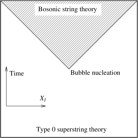
Figure 2: The phase transition from type 0 superstring theory to bosonic string theory. After nucleation of the bubble, the solution interpolates in time between the two theories. Our solution focuses on the upper left-hand corner of the diagram, where the bubble is approximated by a domain wall moving to the left at the speed of light.

Though our initial state is type 0 string theory in $D>10$, one can begin instead from a state with lightlike linear dilaton in the critical dimension, or spacelike linear dilaton in subcritical dimensions. If we have $D=10$ with $\Phi=-{q\over{\sqrt{2}}}\,X^{-}$, or $2\leq D<10$ with $\Phi=qX_{1}$ and $q=\sqrt{{D-10}\over{4{\alpha^{\prime}}{}}}$, we can consider the tachyon profile ${\cal T}=\mu\,{\rm exp}\left(\beta X^{+}\right)$. The physical interpretation may be different from that in $D>10$, but the CFT is equally solvable for all values of $D\geq 2$. For $D=2$, time-dependent tachyon solutions have been studied using the matrix model [10, 11, 12, 13]. Our model is similar to the example of [11], distinguished by our initial state (which is type 0 rather than bosonic string theory, and without a Liouville wall). It would be interesting to study the transition described in this paper using the technology of the matrix model.

We have given a conclusive answer to the question of whether bosonic string theory can be connected with superstring theory by a dynamical realization of the formal embedding of [3]. This possibility has been anticipated (see, for example, [14]). The surprising feature in our model is the essential role of time dependence. It was speculated in [14] that the bosonic string may appear as a stationary but non-static solution of the superstring; the simple scenario we present here realizes bosonic string theory as a type 0 background that is not even stationary.

The achievement of [3] was to prove that all string vacua, even those with distinct worldsheet gauge algebras, can be unified into a single ‘universal string theory.’ For the vacua of bosonic and type 0 strings, we have promoted this formal unification to a physical one, constructing exact, time-dependent solutions that change the effective gauge algebra of the worldsheet. In this context, the moral of our result is clear: The universal string theory is a cosmology. We expect exploration of string dynamics in $D>10$ to yield further surprises.

Appendix

A Generating the canonical transformation from UV to IR fields

The transformation in Eqns. (3.9), (3.11) mixes fields in a nonlinear way, and it is not immediately obvious that the transformation preserves commutators. A simple way to check that a finite change of variables is canonical is to derive the transformation rules from a generating function of the first kind[18]. To see how this works in the case at hand we move to canonical variables, defining conjugate momenta as derivatives of the action:

$$\begin{array}[]{cc}{\bf q}^{+}\equiv X^{+}\ ,&{\bf q}_{-}\equiv\delta_{X^{-}}{\cal L}=-{1\over{2\pi{\alpha^{\prime}}{}}}\dot{X}^{+}\ ,\\ &\\ {\bf Q}^{-}\equiv\delta_{Y^{+}}{\cal L}=-{1\over{2\pi{\alpha^{\prime}}{}}}\dot{Y}^{-}\ ,&{\bf Q}_{+}\equiv Y^{-}\ .\end{array}$$ (A.4)

This translates into the following conjugate momenta:

$$\begin{array}[]{cc}{\bf p}_{+}=\delta_{X^{+}}{\cal L}=-{1\over{2\pi{\alpha^{\prime}}{}}}\dot{X}^{-}\ ,&\quad{\bf p}^{-}=-X^{-}\ ,\\ &\\ {\bf P}_{-}=-Y^{+}\ ,&{\bf P}^{+}=\delta_{Y^{-}}{\cal L}\ .\end{array}$$ (A.8)

We also obtain fermionic canonical coordinates, and momenta as derivatives of the action acting from the left:

$$\begin{array}[]{cc}{\bf q}\equiv\psi^{+}\ ,&\tilde{{\bf q}}\equiv\tilde{\psi}^{+}\ ,\\ &\\ {\bf Q}\equiv c_{4}\ ,&\tilde{{\bf Q}}\equiv\tilde{c}_{4}\ ,\\ &\\ ~{}~{}{\bf p}=+{i\over{2\pi}}\psi^{-}\ ,{}{}&~{}~{}\tilde{{\bf p}}=+{i\over{2\pi}}\tilde{\psi}^{-}\ ,{}{}\\ &\\ {\bf P}=-{i\over{2\pi}}b\ ,&\tilde{{\bf P}}=-{i\over{2\pi}}\tilde{b}\ .\end{array}$$ (A.16)

At this point we can define our canonical transformation using a generating function $F_{1}({\bf q},{\bf Q})$, such that

$${\bf p}_{i}\equiv+{{\delta F_{1}}\over{\delta{\bf q}^{i}}}\ , {\bf P}_{a}\equiv-{{\delta F_{1}}\over{\delta{\bf Q}^{a}}}\ ,$$

$$\tilde{\bf p}\equiv+{{\delta F_{1}}\over{\delta\tilde{\bf q}}}\ , \tilde{\bf P}\equiv-{{\delta F_{1}}\over{\delta\tilde{\bf Q}}}\ ,$$

$${\bf p}\equiv+{{\delta F_{1}}\over{\delta{\bf q}}}\ , {\bf P}\equiv-{{\delta F_{1}}\over{\delta{\bf Q}}}\ ,$$ (A.17)

where all fermionic derivatives are again understood to act from the left. Specifically, our generating function takes the following form

$$F_{1} \equiv \int d\sigma_{1}{\cal F}_{1}\ ,$$

$${\cal F}_{1} \equiv -\frac{1}{2\pi{\alpha^{\prime}}{}}\left(X^{+}\dot{Y}^{-}-\dot{X}^{+}Y^{-}\right)$$ (A.18)

$$-{i\mu\over{2\pi}}{\rm exp}\left(\beta X^{+}\right)\biggl{[}~{}\tilde{\psi}^{+}c_{4}-\psi^{+}\tilde{c}_{4}-(c_{4}\tilde{c}_{4}{}^{\prime}{}-c_{4}{}^{\prime}{}\tilde{c}_{4})-\beta\,\dot{X}^{+}c_{4}\tilde{c}_{4}~{}\biggr{]}$$

$$= {\bf q}^{+}{\bf Q}^{-}-{\bf q}_{-}{\bf Q}_{+}$$

$$-{i\mu\over{2\pi}}{\rm exp}\left(\beta{\bf q}^{+}\right)\biggl{[}\,{\bf\tilde{q}Q}-{\bf q\tilde{Q}}-({\bf Q\tilde{Q}^{\prime}-Q^{\prime}\tilde{Q}})+2\pi\alpha^{\prime}\beta\,{\bf q}_{-}{\bf Q\tilde{Q}}\,\biggr{]}\ .$$

Following the rules in Eqn. (A.17), we obtain eight transformation equations, one for each of the fields $\psi^{+},~{}\psi^{-},~{}\tilde{\psi}^{+},~{}\tilde{\psi}^{-},~{}b,~{}\tilde{b},~{}Y^{+},~{}Y^{-}$. These comprise a system of equations that can be solved to express all of the lower-case canonical variables in terms of the upper-case canonical variables, or vice-versa. For the $\psi$ fields, we obtain

$$\psi^{+} = 2c^{\prime}_{4}-M^{-1}\tilde{b}_{4}+2\beta(\partial_{+}X^{+})c_{4}\ ,$$

$$\psi^{-} = M\tilde{c}_{4}\ ,$$

$$\tilde{\psi}^{+} = -2\tilde{c}^{\prime}_{4}+M^{-1}b_{4}+2\beta(\partial_{-}X^{+})\tilde{c}_{4}\ ,$$

$$\tilde{\psi}^{-} = -Mc_{4}\ .$$ (A.19)

Similarly, the $X$ fields transform according to

$$X^{+} \equiv Y^{+}\ ,$$

$$X^{-} \equiv Y^{-}+i\beta{\alpha^{\prime}}{}\mu\,{\rm exp}\left(\beta X^{+}\right)c_{4}\tilde{c}_{4}\ .$$ (A.20)

Finally, the $b,~{}\tilde{b}$ fields obey

$$b_{4} = -2\beta\partial_{+}X^{+}\psi^{-}+2{\psi^{\prime}}^{-}+M\tilde{\psi}^{+}\ ,$$

$$\tilde{b}_{4} = 2\beta\partial_{+}X^{+}\psi^{-}-2\tilde{\psi^{\prime}}^{-}-M\psi^{+}\ .$$ (A.21)

These are all consistent with the field redefinitions used in Section 3 above, and we conclude that they are proper, canonical transformations.

We are left with a stress tensor and supercurrent describing two free bosons $Y^{\pm}$ and a free $bc$ ghost system with weights $(3/2,-1/2)$. The new equal-time commutators are

$$\{b_{4}(\sigma),c_{4}(\tau)\} = +2\pi\delta(\sigma_{1}-\tau_{1})\ ,$$

$$\{\tilde{b}_{4}(\sigma),\tilde{c}_{4}(\tau)\} = +2\pi\delta(\sigma_{1}-\tau_{1})\ ,$$

$$\left[\partial_{\pm}Y^{\mu}(\sigma),\partial_{\pm}Y^{\nu}(\tau)\right] = -\pi i{\alpha^{\prime}}{}\eta^{\mu\nu}\delta{}^{\prime}{}(\sigma_{1}-\tau_{1})\ ,$$ (A.22)

and the rest vanish.

B OPEs in the interacting $2D$ theory

In this appendix we record a number of OPEs that are needed to compute quantum corrections to the transformations of the stress tensor and supercurrent under the transformation (3.14).

B.1 Solving for the OPE of $\psi^{-}$ with $\tilde{\psi}^{-}$

To compute the quantum contribution to the central charge, we will need to give a sensible, consistent definition to the composite operators that enter the stress tensor and supercurrent. We define the composite operators of the $X^{\mu},\psi^{\mu},\tilde{\psi}^{\mu}$ theory in terms of the $:\,\,:$ normal ordering prescription, whose properties we list in Section 4.1. However, we have to choose more specific definitions of composite operators involving the fields $Y^{\mu},b_{4},c_{4},\tilde{b}_{4},\tilde{c}_{4}$, as well as $X^{\mu},\psi^{\mu},\tilde{\psi}^{\mu}$.

We begin by solving for the $\psi^{-}(\sigma)\tilde{\psi}^{-}(\tau)$ OPE. To do this, we must rely on the normal ordering prescription for $\psi^{\pm}$. Based on diagrammatic arguments, we see that the OPEs for fields involving a $\psi^{+}$ are unaffected by the interaction terms. So the OPEs for $\psi^{\mp}$ with $\psi^{\pm}$ and $\tilde{\psi}^{\pm}$ with $\tilde{\psi}^{\mp}$ are

$$\psi^{\mp}(\sigma)\psi^{\pm}(\tau)=:\psi^{\mp}(\sigma)\psi^{\pm}(\tau):+{i\over{\tau^{+}-\sigma^{+}}}\ ,$$ (B.1)

$$\tilde{\psi}^{\mp}(\sigma)\tilde{\psi}^{\pm}(\tau)=:\tilde{\psi}^{\mp}(\sigma)\tilde{\psi}^{\pm}(\tau):+{i\over{\tau^{-}-\sigma^{-}}}\ .$$ (B.2)

By acting on Eqn. (B.1) with $-{1\over 2}M(\tau^{+},\tau^{-})$ and using the equation of motion $\partial_{+}\tilde{\psi}^{-}=-{1\over 2}M\psi^{+}$, we can find a first-order partial differential equation for the OPE of $\psi^{-}$ with $\tilde{\psi}^{-}$:

$$\partial_{\tau^{+}}\left(\,\psi^{-}(\sigma)\tilde{\psi}^{-}(\tau)\,\right)=\partial_{\tau^{+}}\left(\,:\psi^{-}(\sigma)\tilde{\psi}^{-}(\tau):\,\right)-{i\over 2}{{M(\tau^{+},\tau^{-})}\over{\tau^{+}-\sigma^{+}}}\ .$$ (B.3)

We can also act on Eqn. (B.2) with $+{1\over 2}M(\sigma^{+},\sigma^{-})$ and use the equation of motion $\partial_{-}\psi^{-}=+{1\over 2}M\tilde{\psi}^{+}$ to obtain

$$\partial_{\sigma^{-}}\left(\,\psi^{-}(\sigma)\tilde{\psi}^{-}(\tau)\,\right)=\partial_{\sigma^{-}}\left(\,:\psi^{-}(\sigma)\tilde{\psi}^{-}(\tau):\,\right)+{i\over 2}{{M(\sigma^{+},\sigma^{-})}\over{\tau^{-}-\sigma^{-}}}\ .$$ (B.4)

Any two simultaneous solutions to Eqns. (B.3) and (B.4) must differ by a bilocal operator depending only on $\sigma^{+}$ and $\tau^{-}$. We would like to find the most general possible OPE that satisfies both the constraints of conformal invariance and equations of motion (B.3, B.4). The basic procedure can be divided into three steps. First, we find a particular OPE satisfying the equation of motion at the level of terms that are singular as $\sigma$ approaches $\tau$. Then, we add a set of terms with smooth dependence on $\sigma-\tau$, so that the equations of motion (B.3, B.4) are satisfied identically. Finally, we construct the full set of possible solutions to the equations (B.3, B.4). Since the equations define a linear, inhomogeneous system of partial differential equations with operator-valued source term, we can start by constructing the general solution to the corresponding system of homogeneous equations. By adding this to our particular solution we find the general solution to (B.3, B.4).

1: Constructing a particular solution for the singular terms

First, we construct a particular simultaneous solution that satisfies Eqns. (B.3, B.4) up to terms that have an infinite number of continuous derivatives as $\sigma\to\tau$. The singular terms in the OPE sum up to

$$\psi^{-}(\sigma)\tilde{\psi}^{-}(\tau) \simeq :\psi^{-}(\sigma)\tilde{\psi}^{-}(\tau):-{i\over 2}\ln{1\over{L^{2}}}\left|(\tau^{+}-\sigma^{+})(\tau^{-}-\sigma^{-})\right|M(\sigma^{+},\tau^{-})$$ (B.5)

$$+\left(\,{\rm smooth~{}as~{}}\sigma\to\tau\,\right)\ ,$$

where $L$ is an arbitrary length scale. It is straightforward to check that the OPE in Eqn. (B.5) satisfies Eqns. (B.3) and (B.4), up to terms smooth as $\sigma\to\tau$.

The singular term in the OPE has a simple representation in terms of the geometry of the Lorentzian worldsheet. Drawing two intersecting light rays from the points of insertion of the operators $\psi^{-},~{}\tilde{\psi}^{-}$, one finds that the two light rays, together with the line joining the points, define a triangle. The logarithm of the area of this triangle is the singular coefficient function in the OPE. The operator being multiplied by this coefficient function is evaluated at the intersection point of the two light rays. This framework is depicted in Fig. 3. This very simple Lorentzian description of the OPE suggests that the Lorentzian worldsheet is the natural setting for the type of CFT of interest, rather than the $2D$ Euclidean continuation.

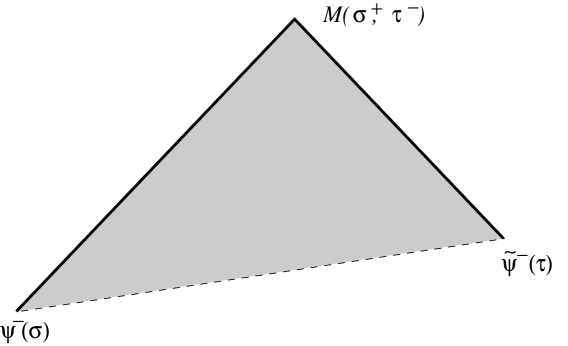
Figure 3: Light rays emerge from the insertion points of $\psi^{-}(\sigma)$ and $\tilde{\psi}^{-}(\tau)$. The operator $M\equiv{\rm exp}\left(\beta X^{+}\right)$ on the right-hand side of the OPE is evaluated at the intersection point $(I)\equiv(\sigma^{+},\tau^{-})$ of the light rays. The coefficient function $\left(\ln\left|\frac{1}{L^{2}}(\tau^{+}-\sigma^{+})(\tau^{-}-\sigma^{-})\right|\right)$ is the logarithm of the area of the triangle formed by the light rays and the line joining the insertion points.

2: Adding smooth terms to satisfy the equations of motion

We can solve for the smooth terms in the OPE as well. One solution to Eqns. (B.3) and (B.4) takes the form

$$\psi^{-}(\sigma)\tilde{\psi}^{-}(\tau) = :\psi^{-}(\sigma)\tilde{\psi}^{-}(\tau):-{i\over 2}\ln\left|{1\over{L^{2}}}(\tau^{+}-\sigma^{+})(\tau^{-}-\sigma^{-})\right|M(\sigma^{+},\tau^{-})$$ (B.6)

$$-{i\over 2}\sum_{n=1}^{\infty}{1\over{n\cdot n!}}\left[\,(\tau^{+}-\sigma^{+})^{n}\,\partial_{+}^{n}+(\sigma^{-}-\tau^{-})^{n}\,\partial_{-}^{n}\,\right]M(\sigma^{+},\tau^{-})\ .$$

The OPE (B.6) identically satisfies the equations of motion, including terms that are smooth as $\sigma$ approaches $\tau$.

3: Constructing the general solution

Any other solution must still satisfy Eqns. (B.3) and (B.4), and therefore must differ from the right-hand side of Eqn. (B.6) by the addition of an operator $\Delta{\cal O}(\sigma,\tau)$, satisfying

$$\partial_{\sigma^{-}}\Delta{\cal O}(\sigma,\tau)=\partial_{\tau^{+}}\Delta{\cal O}(\sigma,\tau)=0\ .$$ (B.7)

We are therefore lead to consider a completely general OPE of two operators, one at $\sigma$ and the other at $\tau$. Any operator on the right-hand side of the OPE can be expressed in the form

$$\sum_{A}{\cal C}_{(A)}^{{\bf 2}}(\sigma-\tau){\cal O}^{(A)}(\tau^{+},\tau^{-})\ ,$$ (B.8)

where the expansion is performed around the location $\tau$ of the second operator on the left-hand side. The right-hand side of the same OPE can be expressed as

$$\sum_{A}{\cal C}_{(A)}^{\rm{\bf 1}}(\sigma-\tau){\cal O}^{(A)}(\sigma^{+},\sigma^{-})\ ,$$ (B.9)

with the expansion around the location $\sigma$ of the first operator on the left-hand side. Since the coefficient functions ${\cal C}_{(A)}^{{\bf 1}}(\sigma-\tau)$ can be rewritten in terms of the coefficient functions ${\cal C}_{(A)}^{\bf 2}(\sigma-\tau)$, we can expand a given OPE around whichever point is most convenient. Of course, we can equally well expand the OPE around the midpoint between the two operators, or around any other point in their vicinity.

Now we would like to parametrize our freedom to change the OPE (B.6) in a way that is consistent with the equations of motion. To do this, let us expand around the point $(I)\equiv(\sigma^{+},\tau^{-})$, where the two light rays emanating from $\sigma$ and $\tau$ intersect (see Fig. 3). We write the additional term $\Delta{\cal O}$ on the right-hand side of our OPE as

$$\Delta{\cal O}(\sigma,\tau)\equiv\sum_{A}{\cal C}_{(A)}^{\rm I}(\sigma-\tau){\cal O}^{(A)}(\sigma^{+},\tau^{-})\ .$$ (B.10)

In terms of the basis of operators at point $(I)$, the condition $\partial_{\sigma^{-}}\Delta{\cal O}=\partial_{\tau^{+}}\Delta{\cal O}=0$ means that the coefficient functions ${\cal C}^{\rm I}_{(A)}(\sigma-\tau)$ must be constants ${\bf C}_{(A)}$. The operator $\Delta{\cal O}(\sigma,\tau)$ is then given by

$$\Delta{\cal O}(\sigma,\tau)\equiv\sum_{A}~{}{\bf C}_{(A)}{\cal O}^{(A)}(\sigma^{+},\tau^{-})\ .$$ (B.11)

Rewriting this as an expansion at $\tau$, we have

$$\Delta{\cal O}(\sigma,\tau)=\sum_{A}~{}\sum_{n=0}{{{\bf C}_{(A)}}\over{n!}}(\sigma^{+}-\tau^{+})^{n}\partial^{n}_{+}{\cal O}^{(A)}(\tau^{+},\tau^{-})\ .$$ (B.12)

Since the operators on the left-hand side of the OPE are $\psi^{-}(\sigma)$ and $\tilde{\psi}^{-}(\tau)$, conformal invariance forces all the ${\cal O}^{(A)}$ to have weight $({1\over 2},{1\over 2})$.

We can further prove that any contribution to the right-hand side of the OPE must scale with $M$ as $M^{+1}$. The only Feynman diagrams that can contribute to this OPE have two untruncated lines labeled $\psi^{-},~{}\tilde{\psi}^{-}$ representing the left-hand side and some number of truncated lines representing the right-hand side. There are no connected diagrams in the theory with more than one interaction vertex. This means that the right-hand side of the OPE scales as $M^{+1}$. The only local operator ${\cal O}^{(A)}$ of weight $({1\over 2},{1\over 2})$ that scales as $M^{+1}$ is $M=\mu\,{\rm exp}\left(\beta X^{+}\right)$ itself.

Since we have not specified the distance scale $L$ in the argument of the logarithm appearing in Eqn. (B.6), the freedom to shift the right-hand side of the OPE by $M(\sigma^{+},\tau^{-})$ is already present in the freedom to choose $L$. Thus, Eqn. (B.6) is already the most general allowed OPE of $\psi^{-}(\sigma)$ with $\tilde{\psi}^{-}(\tau)$.

B.2 Operator product expansion of $X^{-}$ with $\psi^{-}$ and $\tilde{\psi}^{-}$

We can use similar techniques to fix the OPE of $X^{-}$ with $\psi^{-}$. The result must respect conformal invariance and the equations of motion. The OPE must also have only $X^{+}$ and its superpartners on the right-hand side, and the right-hand side must scale as a single power of $M^{+1}$. In this case we will only derive the singular terms.

Using the equation of motion $\partial_{-}\psi^{-}={1\over 2}M\,\tilde{\psi}^{+}$ and the OPE (4.1), we obtain

$$\partial_{\tau^{-}}\left(\,X^{-}(\sigma)\psi^{-}(\tau)\,\right)=\partial_{\tau^{-}}\,\left(\,:X^{-}(\sigma)\psi^{-}(\tau):\,\right)$$

$$\kern 80.0pt+{{\beta{\alpha^{\prime}}{}}\over 4}\ln\left[\,-{1\over{L^{2}}}(\sigma^{+}-\tau^{+})(\sigma^{-}-\tau^{-})\,\right]M(\tau)\tilde{\psi}^{+}(\tau)\ .$$ (B.13)

By then using the equation of motion $\partial_{+}\partial_{-}X^{-}=-i{{\beta{\alpha^{\prime}}{}}\over 4}\,M\tilde{\psi}^{+}\psi^{+}$ and the OPE (B.1), we find

$$\partial_{\sigma^{+}}\partial_{\sigma^{-}}\left(\,X^{-}(\sigma)\psi^{-}(\tau)\,\right) = \partial_{\sigma^{+}}\partial_{\sigma^{-}}\,\left(\,:X^{-}(\sigma)\psi^{-}(\tau):\,\right)$$ (B.14)

$$+{{\beta{\alpha^{\prime}}{}}\over 4}{1\over{\tau^{+}-\sigma^{+}}}M(\sigma^{+},\sigma^{-})\tilde{\psi}^{+}(\sigma)\ .$$

We will only solve the system of equations (B.13), (B.14) up to nonsingular terms. One particular solution that sums all the singular contributions exactly is

$$X^{-}(\sigma)\psi^{-}(\tau) = :X^{-}(\sigma)\psi^{-}(\tau):$$ (B.15)

$$\kern-20.0pt+{{\beta{\alpha^{\prime}}{}}\over 4}\ln\left[\,-{1\over{L^{2}}}(\sigma^{+}-\tau^{+})(\sigma^{-}-\tau^{-})\,\right]\int_{\sigma^{-}}^{\tau^{-}}dyM(\tau^{+},y)\tilde{\psi}^{+}(y)$$

$$\kern-20.0pt+\left(\,{\rm smooth~{}as~{}}\sigma\to\tau\,\right)\ .$$

The right-hand side of the $X^{-}(\sigma)\psi^{-}(\tau)$ OPE can be shifted by a general solution $\Delta{\cal O}_{2}$ to the homogeneous versions of Eqns. (B.13), (B.14):

$$\Delta{\cal O}_{2}=\Delta{\cal O}_{2^{+}}(\tau^{+},\sigma^{+})+\Delta{\cal O}_{2^{-}}(\tau^{+},\sigma^{-})\ .$$ (B.16)

Let us now constrain the OPE by appealing to arguments parallel to those starting with Eqn. (B.10) above. Let us first focus on potential shifts of the right-hand side of the OPE contained in $\Delta{\cal O}_{2^{-}}(\tau^{+},\sigma^{-})$. We can generically expand in local operators around the intersection point $(I^{\prime})\equiv(\tau^{+},\sigma^{-})$:

$$\Delta{\cal O}_{2^{-}}(\tau^{+},\sigma^{-})\equiv\sum_{A}{\cal C}_{(A)}^{\rm I}(\sigma-\tau){\cal O}^{(A)}(\tau^{+},\sigma^{-})\ .$$ (B.17)

By the same arguments below Eqn. (B.10), the coefficient functions ${\cal C}_{(A)}^{\rm I}(\sigma-\tau)$ must be constants, which we again label by ${\bf C}_{(A)}$. Expanding at $\sigma$, we obtain

$$\Delta{\cal O}_{2^{-}}(\tau^{+},\sigma^{-})=\sum_{A}~{}\sum_{n=0}{{{\bf C}_{(A)}}\over{n!}}(\tau^{+}-\sigma^{+})^{n}\partial^{n}_{+}{\cal O}^{(A)}(\sigma)\ .$$ (B.18)

By conformal invariance of the OPE, the weight of ${\cal O}^{(A)}$ must be $(0,{1\over 2})$. However, each ${\cal O}^{(A)}$ must have one factor of $M^{+1}$, as well as an odd number of fermions, making the total weight of each ${\cal O}^{(A)}$ at least $\frac{3}{2}$. We conclude that $\Delta{\cal O}_{2^{-}}(\tau^{+},\sigma^{-})=0$.

Let us now consider contributions from $\Delta{\cal O}_{2^{+}}(\tau^{+},\sigma^{+})$. The operator $\Delta{\cal O}_{2^{+}}$ is bilocal and right-moving in each argument. We can expand $\Delta{\cal O}_{2^{+}}$ in right-moving local operators with coefficient functions depending on the difference $\sigma^{+}-\tau^{+}$. Each term in the expansion has exactly one factor of $M^{+1}$, which has left-moving weight ${1\over 2}$. Any $\partial_{-}$ derivatives contained in the local operators can only increase the left-moving weight, and the coefficient functions in the expansion are independent of the “$-$” coordinates. The left-hand side of the OPE $X^{-}\psi^{-}$ has total left-moving weight zero, so we conclude $\Delta{\cal O}_{2^{+}}(\tau^{+},\sigma^{+})=0$.

Hence, up to smooth terms, we have completely fixed the OPE to be

$$X^{-}(\sigma)\psi^{-}(\tau) \simeq :X^{-}(\sigma)\psi^{-}(\tau):$$ (B.19)

$$\kern-35.0pt+{{\beta{\alpha^{\prime}}{}}\over 4}\ln\left[\,-{1\over{L^{2}}}(\sigma^{+}-\tau^{+})(\sigma^{-}-\tau^{-})\,\right]\int_{\sigma^{-}}^{\tau^{-}}dyM(\tau^{+},y)\tilde{\psi}^{+}(y)\ .$$

For fermions with “$\widetilde{\phantom{A}}$” labels, we can apply the same reasoning to derive the OPE

$$X^{-}(\sigma)\tilde{\psi}^{-}(\tau) \simeq :X^{-}(\sigma)\tilde{\psi}^{-}(\tau):$$ (B.20)

$$\kern-35.0pt-{{\beta{\alpha^{\prime}}{}}\over 4}\ln\left[\,-{1\over{L^{2}}}(\sigma^{+}-\tau^{+})(\sigma^{-}-\tau^{-})\,\right]\int_{\sigma^{+}}^{\tau^{+}}dyM(y,\tau^{-})\psi^{+}(y)\ .$$

As above, the notation $\simeq$ denotes equality up to the addition of smooth terms.

B.3 Solving for the remaining OPEs

We would now like to solve for the OPE between $c_{4}$ and $\tilde{c}_{4}$. We can perform a series of steps analogous to the derivation of the OPE between $\psi^{-}$ and $\tilde{\psi}^{-}$. First, we note that all OPEs involving $b_{4},~{}\tilde{b}_{4}$ are, as usual,

$$b_{4}(\sigma)c_{4}(\tau)\sim+{i\over{\sigma^{+}-\tau^{+}}}\ ,$$

$$\tilde{b}_{4}(\sigma)\tilde{c}_{4}(\tau)\sim+{i\over{\sigma^{-}-\tau^{-}}}\ ,$$ (B.21)

with no other singular terms. As described in Section 4, we define a normal ordering prescription ${{\circ}\atop{\circ}}{\cal O}_{1}{\cal O}_{2}{{\circ}\atop{\circ}}$ that subtracts the singularity whenever one of the operators involved is $b_{4},\tilde{b}_{4}$ or $Y^{+}$:

$$b_{4}(\sigma)c_{4}(\tau)={{\circ}\atop{\circ}}b_{4}(\sigma)c_{4}(\tau){{\circ}\atop{\circ}}+{i\over{\sigma^{+}-\tau^{+}}}\ ,$$

$$\tilde{b}_{4}(\sigma)\tilde{c}_{4}(\tau)={{\circ}\atop{\circ}}\tilde{b}_{4}(\sigma)\tilde{c}_{4}(\tau){{\circ}\atop{\circ}}+{i\over{\sigma^{-}-\tau^{-}}}\ .$$ (B.22)

The consistency of this prescription follows from the structure of the Feynman diagrams in the $b_{4}c_{4}$ theory, where the Lagrangian has oriented propagators (flowing from $b_{4},~{}\tilde{b}_{4}$ to $c_{4},~{}\tilde{c}_{4}$ and $Y^{+}$ to $Y^{-}$). These propagators are displayed in Fig. 4. As a consequence, interaction vertices have only outgoing lines, as shown in Fig. 5. (It should be emphasized that the absence of loop contributions to interaction diagrams holds for both the infrared as well as the ultraviolet systems.)

Figure 4: Propagators in the $b_{4},~{}c_{4}$ theory are oriented, flowing from $b_{4},~{}\tilde{b}_{4}$ to $c_{4},~{}\tilde{c}_{4}$ (left panel), and from $Y^{+}$ to $Y^{-}$ (right panel).

Figure 5: Because the propagators in the theory are oriented, all interaction vertices are composed strictly of outgoing lines. This is true for both the infrared and ultraviolet theories.

Since the operators $b_{4},~{}\tilde{b}_{4}$ are related to $c_{4},~{}\tilde{c}_{4}$ by differential equations, we can write a system of equations for the OPE $c_{4}(\sigma)\tilde{c}_{4}(\tau)$, and solve it as we did for the OPE $\psi^{-}(\sigma)\tilde{\psi}^{-}(\tau)$. Defining

$$N(\sigma)\equiv M^{-1}(\sigma)={1\over\mu}{\rm exp}\left(-\beta X^{+}\right)\ ,$$ (B.23)

the resulting OPE takes the form

$$c_{4}(\sigma)\tilde{c}_{4}(\tau) = {{\circ}\atop{\circ}}c_{4}(\sigma)\tilde{c}_{4}(\tau){{\circ}\atop{\circ}}-{i\over 2}\ln\left|{1\over{L^{\prime 2}}}(\tau^{+}-\sigma^{+})(\tau^{-}-\sigma^{-})\right|N(\sigma^{+},\tau^{-})$$ (B.24)

$$- {i\over 2}\sum_{n=1}^{\infty}{1\over{n\cdot n!}}\left[\,(\tau^{+}-\sigma^{+})^{n}\,\partial_{+}^{n}+(\sigma^{-}-\tau^{-})^{n}\,\partial_{-}^{n}\,\right]N(\sigma^{+},\tau^{-})\ .$$

This is the unique solution to the OPE for $c_{4}$ with $\tilde{c}_{4}$ that satisfies the equations of motion and the constraints of conformal invariance. The only freedom in the solution is the freedom to choose the length scale $L{}^{\prime}{}$.

There is also a logarithmic correction to the OPE of $Y^{-}$ with $c_{4}$ and $\tilde{c}_{4}$, proportional to $N(\sigma)$. Making use of the same techniques employed in Section B.2, we find:

$$Y^{-}(\sigma)c_{4}(\tau) \simeq {{\circ}\atop{\circ}}Y^{-}(\sigma)c_{4}(\tau){{\circ}\atop{\circ}}$$ (B.25)

$$\kern-25.0pt+{{\beta{\alpha^{\prime}}{}}\over 4}\ln\left[\,-{1\over{L^{\prime 2}}}(\sigma^{+}-\tau^{+})(\sigma^{-}-\tau^{-})\,\right]\int_{\sigma^{-}}^{\tau^{-}}dyN(\tau^{+},y)\tilde{b}_{4}(y)\ ,$$

$$Y^{-}(\sigma)\tilde{c}_{4}(\tau) \simeq {{\circ}\atop{\circ}}Y^{-}(\sigma)\tilde{c}_{4}(\tau){{\circ}\atop{\circ}}$$ (B.26)

$$\kern-25.0pt-{{\beta{\alpha^{\prime}}{}}\over 4}\ln\left[\,-{1\over{L^{\prime 2}}}(\sigma^{+}-\tau^{+})(\sigma^{-}-\tau^{-})\,\right]\int_{\sigma^{+}}^{\tau^{+}}dyN(y,\tau^{-})b_{4}(y)\ ,$$

modulo the addition of smooth terms.

B.4 Quantum change of variables for composite operators

Having established corrections to the OPEs involving the basic fields in both the infrared and ultraviolet variables, we now present some OPEs involving combinations of fields that will be directly relevant to the renormalization of the stress tensor. Given our normal ordering definitions, we can apply the change of variables in Eqns. (3.11) and (3.14) to composite operators. We thus calculate the quantum corrections in four steps. First, we begin by defining normal-ordered composite operators in the ultraviolet fields, written as $\sigma\to\tau$ limits of unordered products of separated fields, with singularities subtracted explicitly. Second, we write the unordered products of ultraviolet fields, for finite $\sigma-\tau$, in terms of the infrared fields, applying the change of variables in Eqn. (3.14). The resulting expression is an unordered product of infrared variables at separated points $\sigma,~{}\tau$ with a singularity subtracted. Third, we use the OPE of the infrared description to rewrite the product in terms of normal-ordered ${{\circ}\atop{\circ}}\,\,{{\circ}\atop{\circ}}$ products. Finally, we take the limit $\sigma\to\tau$.

If carried out correctly, the above steps always take a nonsingular expression in the ultraviolet variables to a nonsingular expression in the infrared variables. As an example, we can compute the transformation of the composite operator $:\psi^{+}(\sigma)\partial_{+}\psi^{-}(\sigma):$. Carrying out the above steps explicitly, we rewrite the expression as

$$\lim_{\sigma\to\tau}~{}\partial_{\tau^{+}}\left(\,\psi^{+}(\sigma)\psi^{-}(\tau)-{i\over{\tau^{+}-\sigma^{+}}}\,\right)\ .$$

For convenience, we can simply calculate the transformation of $:\psi^{+}(\sigma)\psi^{-}(\tau):$ directly, differentiating with respect to $\tau^{+}$ before taking the limit $\sigma\to\tau$.

We next rewrite the combination $\psi^{+}(\sigma)\psi^{-}(\tau)-{i\over{\tau^{+}-\sigma^{+}}}$ as

$$-{i\over{\tau^{+}-\sigma^{+}}}+2\biggl{[}\partial_{+}c_{4}(\sigma)+\beta(\partial_{+}X^{+})(\sigma)c_{4}(\sigma)\biggr{]}\left(\,M(\tau)\tilde{c}_{4}(\tau)\,\right)\ .$$

We now refer to the OPE of $c_{4}(\sigma)$ with $\tilde{c}_{4}(\tau)$ (B.24) and expand about small separations $\epsilon^{\pm}\equiv\sigma^{\pm}-\tau^{\pm}$:

$$c_{4}(\sigma)\tilde{c}_{4}(\tau) = {{\circ}\atop{\circ}}c_{4}(\sigma)\tilde{c}_{4}(\tau){{\circ}\atop{\circ}}$$ (B.27)

$$-{{i}\over 2}\ln\left|\epsilon^{+}\epsilon^{-}/L^{\prime 2}\right|\cdot\left(\,N(\tau)+\epsilon^{+}\partial_{+}N(\tau)+{1\over 2}\epsilon^{+2}\partial_{+}^{2}N(\tau)\,\right)$$

$$+{{i}\over 2}\left(\,\epsilon^{+}\partial_{+}N(\tau)+{3\over 4}\partial_{+}^{2}N(\tau)\epsilon^{+2}\,\right)$$

$$+{{i}\over 2}\epsilon^{-}\left(\,-\partial_{-}N(\tau)-\epsilon^{+}\partial_{+}\partial_{-}N(\tau)-{1\over 4}\epsilon^{-}\partial_{-}^{2}N(\tau)\,\right)+O(\epsilon^{3})\ .$$

Using this, we rewrite the operator as

$$:\psi^{+}(\sigma)\psi^{-}(\tau):=2~{}{{\circ}\atop{\circ}}\left(\,\partial_{+}c_{4}(\sigma)+\beta\partial_{+}X^{+}(\sigma)c_{4}(\sigma)\,\right)\,\tilde{c}_{4}(\tau)M(\tau){{\circ}\atop{\circ}}$$

$$-i\beta(\sigma^{+}-\tau^{+})\partial^{2}_{+}X^{+}(\tau)+O((\sigma-\tau)^{2})\ .$$ (B.28)

In particular, we find that the singularity is canceled. As our final step, we take a derivative with respect to $\tau^{+}$ and find the limit as $\sigma\to\tau$. We are left with

$$:\psi^{+}(\partial_{+}\psi^{-}):={{\circ}\atop{\circ}}(\partial_{+}c_{4}+\beta c_{4}\partial_{+}X^{+})(b_{4}+2\beta M\tilde{c}_{4}\partial_{+}X^{+}){{\circ}\atop{\circ}}+i\beta\partial_{+}^{2}X^{+}\ .$$ (B.29)

Applying the change of variables in Eqn. (3.14) as a classical field transformation yields the first term in Eqn. (B.29), but not the second. We should therefore think of $\beta\partial_{+}^{2}X^{+}$ as a quantum correction to the transformation of $:\psi^{+}\partial_{+}\psi^{-}:$.

B.5 Transformation of the stress tensor and supercurrent

Using the algorithm described above, we can transform the various terms in the stress tensor, including quantum corrections. The quadratic term in the stress tensor $T^{X^{\mu}}$ transforms as

$${2\over{{\alpha^{\prime}}{}}}\,:(\partial_{+}X^{+})(\partial_{-}X^{-}): = {2\over{{\alpha^{\prime}}{}}}\,{{\circ}\atop{\circ}}(\partial_{+}Y^{+})(\partial_{-}Y^{-}){{\circ}\atop{\circ}}+2i\beta^{2}M(\partial_{+}X^{+})^{2}{{\circ}\atop{\circ}}c_{4}\tilde{c}_{4}{{\circ}\atop{\circ}}$$ (B.30)

$$+2i\beta M\partial_{+}X^{+}{{\circ}\atop{\circ}}\partial_{+}c_{4}\tilde{c}_{4}{{\circ}\atop{\circ}}+i\beta\partial_{+}X^{+}{{\circ}\atop{\circ}}c_{4}b_{4}{{\circ}\atop{\circ}}\ ,$$

with no quantum correction relative to that which is obtained by classical substitution of Eqn. (3.14) alone. The linear dilaton term $V_{\mu}\partial_{+}^{2}X^{\mu}$ transforms straightforwardly, again with no quantum correction:

$${\alpha^{\prime}}{}V_{\mu}\partial_{+}^{2}X^{\mu} = V_{\mu}\partial_{+}^{2}Y^{\mu}-i~{}{{\circ}\atop{\circ}}\Bigl{(}\beta^{2}(\partial_{+}Y^{+})^{2}Mc_{4}\tilde{c}_{4}+\beta(\partial_{+}^{2}Y^{+})Mc_{4}\tilde{c}_{4}$$ (B.31)

$$+Mc_{4}^{\prime\prime}{}\tilde{c}_{4}+2\beta M(\partial_{+}Y^{+})(\partial_{+}c_{4})\tilde{c}_{4}$$

$$+{1\over 2}c_{4}(\partial_{+}b_{4})+(\partial_{+}c_{4})b_{4}+{1\over 2}\beta(\partial_{+}Y^{+})c_{4}b_{4}\Bigr{)}{{\circ}\atop{\circ}}\ .$$

The only terms whose transformation receives a quantum correction are the terms in the fermionic stress tensor $T^{\psi^{\mu}}$ in (3.2).

The normal-ordered product of the two $\psi$ fermions is given in Eqn. (B.29). Differentiating and taking the limit $\sigma\to\tau$, we derive the quantum-corrected transformations for the fermion terms in the stress tensor:

$$-{i\over 2}:\psi^{-}(\partial_{+}\psi^{+}):-{i\over 2}:\psi^{+}(\partial_{+}\psi^{-}): = -{i\over 2}~{}{{\circ}\atop{\circ}}\Bigl{(}(\partial_{+}c_{4})b_{4}+\beta\partial_{+}X^{+}c_{4}b_{4}$$ (B.32)

$$\kern-180.0pt+2\beta^{2}(\partial_{+}X^{+})\,M\,^{2}c_{4}\tilde{c}_{4}-2M(\partial_{+}^{2}c_{4})\tilde{c}_{4}-2\beta M\partial_{+}^{2}X^{+}c_{4}\tilde{c}_{4}\Bigr{)}{{\circ}\atop{\circ}}+\beta\partial_{+}^{2}X^{+}\ .$$

Summing the various remaining terms in the stress tensor, we find

$${T^{\rm LC}} \equiv T^{X^{\mu}}+T^{\psi^{\mu}}\ ,$$

$$T^{Y^{\mu}}+T^{\psi^{\mu}} = -\frac{1}{\alpha^{\prime}}G_{\mu\nu}\partial_{+}Y^{\mu}\partial_{+}Y^{\nu}+V_{\mu}\partial^{2}Y^{\mu}$$ (B.33)

$$-\frac{3i}{2}\partial_{+}c_{4}\,b_{4}-\frac{i}{2}c_{4}\,\partial_{+}b_{4}+\beta\partial_{+}^{2}X^{+}\ .$$

The supercurrent in ultraviolet variables is naturally decomposed into four pieces, written explicitly in Eqn. (4.17) above. Of the four pieces, only ${\bf 1}$ receives a quantum correction to its classical transformation under the change of variables. To transform ${\bf 1}$ with quantum corrections included, we make use of the OPE

$$(\partial_{+}X^{-}(\sigma))\psi^{+}(\tau) = 2~{}{{\circ}\atop{\circ}}\partial_{\sigma^{+}}\left(\,Y^{-}(\sigma)+i\beta{\alpha^{\prime}}{}M(\sigma)c_{4}(\sigma)\tilde{c}_{4}(\sigma)\,\right)$$ (B.34)

$$\kern 0.0pt\times\left(\,\partial_{+}c_{4}(\sigma)+\beta\partial_{+}Y^{+}(\tau)c_{4}(\tau)\,\right){{\circ}\atop{\circ}}$$

$$\kern-40.0pt+{{\beta{\alpha^{\prime}}{}}\over 2}\,\partial_{+}^{2}c_{4}(\sigma)+\beta^{2}{\alpha^{\prime}}{}c_{4}(\sigma)\partial_{+}^{2}Y^{+}(\sigma)+O(\sigma-\tau)+O(M^{-1})\ ,$$

which we derived according to the rules in Section B.4. The term ${\bf 1}$ in the supercurrent then transforms into ${\bf 1}_{\rm classical}+{\bf 1}_{\rm quantum}$, where

$${\bf 1}_{\rm classical} = -2\sqrt{2\over{\alpha^{\prime}}{}}{{\circ}\atop{\circ}}\partial_{+}\left(\,Y^{-}+i\beta{\alpha^{\prime}}{}Mc_{4}\tilde{c}_{4}\,\right)\left(\,\partial_{+}c_{4}+\beta\partial_{+}Y^{+}c_{4}\,\right){{\circ}\atop{\circ}}\ ,$$

$${\bf 1}_{\rm quantum} = -\beta\sqrt{{{{\alpha^{\prime}}{}}\over 2}}\partial_{+}^{2}{c_{4}}-2\beta^{2}\sqrt{{{{\alpha^{\prime}}{}}\over 2}}c_{4}\partial_{+}^{2}Y^{+}\ .$$ (B.35)

The remaining three parts are given simply by classical substitution, because the corresponding operator products have no singularities from the interaction terms:

$${\bf 2} = -\sqrt{2\over{\alpha^{\prime}}{}}M(\partial_{+}Y^{+})\tilde{c}_{4}\ ,$$

$${\bf 3} = 2q\sqrt{{\alpha^{\prime}}{}}(\partial_{+}^{2}c_{4})+2\beta q\sqrt{{\alpha^{\prime}}{}}(\partial_{+}Y^{+})(\partial_{+}c_{4})+2\beta q\sqrt{{\alpha^{\prime}}{}}c_{4}(\partial_{+}^{2}Y^{+})\ ,$$

$${\bf 4} = q\sqrt{{\alpha^{\prime}}{}}M~{}(\partial_{+}\tilde{c}_{4})+q\sqrt{{\alpha^{\prime}}{}}\beta\tilde{c}_{4}~{}M(\partial_{+}Y^{+})\ .$$ (B.36)

Using fermi statistics, the equations of motion for $\tilde{c}_{4}$, and the relation $\beta q={{\sqrt{2}}\over{{\alpha^{\prime}}{}}}$, we recover a form of the supercurrent that is manifestly finite in the limit $M\to\infty$. The various terms appear as

$${\bf 1}_{\rm classical} = -2\sqrt{2\over{{\alpha^{\prime}}{}}}~{}{{\circ}\atop{\circ}}\left[\,(\partial_{+}c_{4})(\partial_{+}Y^{-})+\beta c_{4}(\partial_{+}Y^{+})(\partial_{+}Y^{-})-{{i\beta{\alpha^{\prime}}{}}\over 2}(\partial_{+}c_{4})b_{4}c_{4}\,\right]{{\circ}\atop{\circ}}\ ,$$

$${\bf 1}_{\rm quantum} = -\beta\sqrt{{{{\alpha^{\prime}}{}}\over 2}}\partial_{+}^{2}{c_{4}}-2\beta^{2}\sqrt{{{{\alpha^{\prime}}{}}\over 2}}c_{4}\partial_{+}^{2}Y^{+}\ ,$$

$${\bf 2}+{\bf 4} = {q\over 2}\sqrt{{\alpha^{\prime}}{}}b_{4}\ ,$$

$${\bf 3} = 2q\sqrt{{\alpha^{\prime}}{}}(\partial_{+}^{2}c_{4})+2\sqrt{2\over{\alpha^{\prime}}{}}(\partial_{+}Y^{+})(\partial_{+}c_{4})+2\sqrt{2\over{\alpha^{\prime}}{}}c_{4}(\partial_{+}^{2}Y^{+})\ .$$

C BRST cohomology in the Berkovits-Vafa formalism

To show that the Berkovits-Vafa formalism is equivalent to the usual formulation of the bosonic string, one can use a local operator transformation that puts the BRST current into a form that makes the equivalence manifest. We note that in this appendix we refer to the usual $\beta\gamma$ Fadeev-Popov ghost system using the conventional notation. The reader should take care not to confuse the $\beta$ ghost with the lightlike Liouville exponent $\beta$, which plays no role in this appendix.

The BRST current of the Berkovits-Vafa formalism is of the same form as any other superstring theory in covariant gauge. It is convenient to break quantities into matter and reparametrization ghost sectors. We use the notation $b_{\rm fp}$ and $c_{\rm fp}$ to denote the Fadeev-Popov $bc$ ghost system. As noted, the $\beta\gamma$ system will be denoted in the standard way. The BRST current appears as

$$J_{\rm BRST}=c_{\rm fp}\left(\,{T}^{({\rm mat}+b_{1}c_{1})}+{1\over 2}T^{\rm gho}\,\right)+\gamma\left(\,G^{\rm bv}+{1\over 2}G^{\rm gho}\,\right)\ ,$$ (C.1)

where

$$T^{\rm gho} \equiv -i(\partial_{+}b_{\rm fp})c_{\rm fp}-2ib_{\rm fp}(\partial_{+}c_{\rm fp})-{1\over 2}(\partial_{+}\beta)\gamma-{3\over 2}\beta(\partial_{+}\gamma)\ ,$$

$$G^{\rm gho} \equiv (\partial_{+}\beta)c_{\rm fp}+{3\over 2}\beta(\partial_{+}c_{\rm fp})-2b_{\rm fp}\gamma\ ,$$

$${T}^{({\rm mat}+b_{1}c_{1})} \equiv T^{\rm mat}+T^{b_{1}c_{1}}\ ,$$ (C.2)

and $G^{\rm bv}$ is the Berkovits-Vafa supercurrent (5.26); here we use the explicit label “bv” to distinguish this supercurrent from that of the ghost (gho) sector. The notation ${T}^{({\rm mat}+b_{1}c_{1})}$ is meant to indicate the full stress tensor $T^{\rm mat}+T^{b_{1}c_{1}}$ appropriate for a $c=15$ SCFT.

The transformation we seek is generated by a Hermitian generator $h$ (here and throughout this subsection, normal ordering is implied unless otherwise specified):

$$h \equiv +{1\over{2\pi}}\int d\sigma_{1}\Bigl{[}{1\over 2}b_{\rm fp}c_{\rm fp}(\partial_{+}c_{1})c_{1}-ib_{\rm fp}\gamma c_{1}-{i\over 4}\beta\gamma(\partial_{+}c_{1})c_{1}$$ (C.3)

$$-ic_{\rm fp}\beta(\partial_{+}c_{1})+\frac{i}{2}(\partial_{+}c_{\rm fp})\beta c_{1}\Bigr{]}\ .$$

Defining the unitary operator $U\equiv{\rm exp}\left(ih\right)$, we can transform the dynamical variables of the theory into a set of variables in which the BRST current assumes a simple form. In particular, the $\beta,\gamma,b_{1},c_{1}$ fields are decoupled from the remaining degrees of freedom, in transformed variables.

For completeness, we record the OPEs of the $b_{\rm fp},c_{\rm fp},\beta,\gamma$ and ${b_{1}},{c_{1}}$ fields:

$$b_{\rm fp}(\sigma)c_{\rm fp}(0) \sim -\frac{i}{\sigma^{+}+i\epsilon}\ ,$$

$${b_{1}}(\sigma){c_{1}}(0) \sim +\frac{i}{\sigma^{+}+i\epsilon}\ ,$$

$$\beta(\sigma)\gamma(0) \sim -\frac{1}{\sigma^{+}+i\epsilon}\ .$$ (C.4)

The transformation of the BRST current of the full theory is thus obtained as follows:

$$J_{\rm BRST}^{{\rm new}} \equiv U\,J_{\rm BRST}\,U^{-1}$$ (C.5)

$$= J_{\rm BRST}^{{\rm mat}}+J_{\rm BRST}^{{\rm quartet}}+J_{\rm BRST}^{{\rm deriv}}\ ,$$

where we have defined

$$J_{\rm BRST}^{{\rm mat}} \equiv cT^{{\rm mat}}-i:b(\partial_{+}c)c:+{3\over 2}\partial_{+}^{2}c\ ,$$

$$J_{\rm BRST}^{{\rm quartet}} \equiv b_{1}\gamma\ ,$$

$$J_{\rm BRST}^{{\rm deriv}} \equiv \partial_{+}\Bigl{(}-{i\over 4}b_{\rm fp}c_{\rm fp}\gamma c_{1}-{1\over 4}\beta\gamma^{2}c_{1}+{i\over 2}c_{\rm fp}b_{1}c_{1}-{3\over 4}c_{\rm fp}\beta\gamma-{i\over 8}c_{\rm fp}\beta\gamma(\partial_{+}c_{1})c_{1}$$ (C.6)

$$-{{11i}\over{16}}c_{\rm fp}(\partial_{+}^{2}c_{1})c_{1}-{5\over 4}\gamma(\partial_{+}c_{1})+{{3i}\over 8}(\partial_{+}c_{\rm fp})c_{\rm fp}\beta c_{1}$$

$$-{{5i}\over 8}(\partial_{+}c_{\rm fp})(\partial_{+}c_{1})c_{1}-{1\over 2}(\partial_{+}c_{\rm fp})\Bigr{)}\ .$$

The term $J_{\rm BRST}^{{\rm deriv}}$ is a total derivative, and does not contribute to the integrated BRST charge. The other two terms integrate to two anticommuting BRST operators $Q_{\rm BRST}^{{\rm mat}}$ and $Q_{\rm BRST}^{{\rm quartet}}$. The BRST cohomology in the ‘decoupled’ variables must therefore decompose into states of the form $\left|{{{\rm mat}}}\right\rangle\otimes\left|{{\rm quartet}}\right\rangle$, where $\left|{{{\rm mat}}}\right\rangle$ and $\left|{{\rm quartet}}\right\rangle$ are in the cohomology of $Q_{\rm BRST}^{{\rm mat}}$ and $Q_{\rm BRST}^{\rm quartet}$, respectively.

The cohomology of $Q_{\rm BRST}^{{\rm mat}}$ is well-known: it consists of operators of the form $c_{\rm fp}V^{{\rm mat}}$ and $c_{\rm fp}(\partial_{+}c_{\rm fp})V^{{\rm mat}}$, where $V^{{\rm mat}}$ is a Virasoro primary of weight one. The latter, as usual, do not define physical states but rather the set of ‘covectors’ that have natural inner products with the usual physical states [19].

The cohomology of $Q_{\rm BRST}^{{\rm quartet}}$ is straightforward to calculate, since the operator is exactly quadratic in free fields. The cohomology depends only on the ‘picture’ in which the state is built: that is, the smallest number $n$ such that $\gamma_{n+{3\over 2}}$ acts as an annihilation operator and $\beta_{-(n+{3\over 2})}$ acts as a creation operator. So in particular, the entire cohomology in the 0 picture of the $b_{1},c_{1},\beta,\gamma$ sector is exhausted by the identity operator $1$. The cohomology in the $-1$ picture is exhausted by the operator $c_{1}\delta(\gamma)$. The cohomology in the $-2$ picture is exhausted by $c_{1}(\partial_{+}c_{1})\delta(\gamma)\delta(\partial_{+}\gamma)$. In each case, the entire cohomology consists of a single state, which can be represented as the product of a state in the $\beta,\gamma$ sector with a state in the $b_{1},c_{1}$ sector. The state of the $\beta,\gamma$ sector is a generalized ‘vacuum’, defined as the state annihilated by all the annihilation operators $\gamma_{{\rm picture}+m+{3\over 2}},~{}\beta_{m-{1\over 2}-{\rm picture}}$ for $m\geq 0$. The state of the $b_{1},c_{1}$ sector is the state of lowest weight whose value of $n_{b_{1}}-n_{c_{1}}$ is equal to the picture of the state.

The total ghost number $n_{c_{\rm fp}}+n_{\gamma}-n_{b_{\rm fp}}-n_{\beta}$ is a grading respected by the BRST charge (which has ghost number $+1$) and also by our unitary transformation $U\equiv{\rm exp}\left(ih\right)$, since $h$ has ghost number zero. It is therefore useful to classify the BRST cohomology by ghost number. (We count the Berkovits-Vafa fields $b_{1},c_{1}$ as having ghost number zero.) For every value $m$ of the ghost number, there are exactly two kinds of BRST cohomology classes, each built from a matter vertex operator $V_{{\rm mat}}$ that is a primary of weight one with respect to $T^{{\rm mat}}$. The first set is of the form

$$c_{\rm fp}V_{{\rm mat}}{\cal O}_{m-1}\ ,$$ (C.7)

while the second set is of the form

$$c_{\rm fp}(\partial_{+}c_{\rm fp})V_{{\rm mat}}{\cal O}_{m-2}\ .$$ (C.8)

${\cal O}_{m}$ is the picture $m$ vacuum of the $b_{1},c_{1},\beta,\gamma$ system, which is proportional to

$${\cal O}_{m<0}\equiv\prod_{j=0}^{-m-1}(\partial^{j}_{+}c_{1})\delta(\partial_{+}^{j}\gamma)\ ,$$ (C.9)

for negative $m$, or

$${\cal O}_{m>0}\equiv\prod_{j=0}^{m-1}(\partial^{j}_{+}b_{1})\delta(\partial_{+}^{j}\beta)\ ,$$ (C.10)

for positive $m$, and is proportional to the identity for $m=0$.

Because the picture zero cohomology is just the identity, we know that the cohomology at picture $-m$ must consist entirely of the $m^{\rm th}$ power of the inverse picture changing operator, defined by [20, 21]

$$Y\equiv c_{\rm fp}\delta^{\prime}(\gamma)\ .$$ (C.11)

In decoupled variables, this operator appears as

$$Y_{{\rm decoupled}}=-c_{1}\delta(\gamma)\ ,$$ (C.12)

up to terms that are BRST trivial. More explicitly, the two are related by

$$U\,Y\,U^{-1} = c_{\rm fp}\delta^{\prime}(\gamma)-c_{1}\delta(\gamma)+\frac{i}{2}(\partial_{+}c_{\rm fp})c_{\rm fp}c_{1}\delta^{\prime\prime}(\gamma)$$ (C.13)

$$\equiv Y_{{\rm decoupled}}-\frac{i}{2}Q_{\rm BRST}^{\rm decoupled}\left(c_{\rm fp}c_{1}\delta^{\prime\prime}(\gamma)\right)\ ,$$

where we have defined $Q_{\rm BRST}^{\rm decoupled}=Q^{{\rm mat}}_{\rm BRST}+Q^{{\rm quartet}}_{\rm BRST}$. In the other direction,

$$U^{-1}Y_{{\rm decoupled}}U = -Y-\frac{i}{2}Q_{\rm BRST}\left(\,c_{\rm fp}c_{1}\delta^{\prime\prime}(\gamma)\,\right)\ .$$ (C.14)

Starting with a vertex operator in the decoupled variables in $-1$ picture

$$c_{\rm fp}c_{1}\delta(\gamma)V_{{\rm mat}}\ ,$$ (C.15)

it is straightforward (in fact, trivial) to translate to the usual Berkovits-Vafa framework. The generator $h$ commutes with $V_{{\rm mat}}$, as well as with any operator of the form $c_{\rm fp}c_{1}f(\gamma)$, so the form of the $-1$ picture physical state vertex operator is unchanged.

The situation is slightly more complicated when starting from another picture. For example, the picture zero vertex operator $c_{\rm fp}V_{{\rm mat}}$ does not commute with the generator $h$, and it has a nontrivial (inverse) transformation to the standard Berkovits-Vafa theory. However, we know explicit forms for all physical states and dual physical states in every picture in the decoupled variables. For instance, the physical state and its dual in picture zero are $c_{\rm fp}V_{{\rm mat}}$ and $(\partial_{+}c_{\rm fp})c_{\rm fp}V_{{\rm mat}}$, respectively. Explicitly, The inverse transformation defined by the unitary operator $U$ appears as

$$U^{-1}\,c_{\rm fp}V_{{\rm mat}}\,U = c_{\rm fp}V_{{\rm mat}}-\gamma c_{1}V_{{\rm mat}}\ ,$$

$$U^{-1}\,(\partial_{+}c_{\rm fp})c_{\rm fp}V_{{\rm mat}}\,U = \Bigl{(}c_{\rm fp}(\partial_{+}c_{1})\gamma+c_{\rm fp}c_{1}(\partial_{+}\gamma)+\gamma^{2}(\partial_{+}c_{1})c_{1}$$ (C.16)

$$\kern 30.0pt+(\partial_{+}c_{\rm fp})c_{\rm fp}-(\partial_{+}c_{\rm fp})c_{1}\gamma\Bigr{)}V_{{\rm mat}}\ .$$

The physical states and dual physical states at picture $-1$ transform trivially:

$$U^{-1}\,c_{\rm fp}c_{1}\delta(\gamma)V_{{\rm mat}}\,U = c_{\rm fp}c_{1}\delta(\gamma)V_{{\rm mat}}\ ,$$

$$U^{-1}\,(\partial_{+}c_{\rm fp})c_{\rm fp}c_{1}\delta(\gamma)V_{{\rm mat}}\,U = (\partial_{+}c_{\rm fp})c_{\rm fp}c_{1}\delta(\gamma)V_{{\rm mat}}\ .$$ (C.17)

These objects exhaust the BRST cohomology at pictures 0 and 1 in the Berkovits-Vafa string. We will use our knowledge of the full BRST cohomology in the next subsection.

D Ramond sectors

The late-time limit of our model differs from the formulation of [3] in one respect. In the usual framework of [3], all operators in the sector ${T}^{({\rm mat}+b_{1}c_{1})}$ are neutral under the GSO projection, and all fields have their usual periodicity in the Ramond sectors, except for the $b_{1}c_{1}$ fields. The result is that, in [3], there are no physical states in the R/R sector. The R/R sector has four vacua, but the one that obeys the physical state conditions $G_{0}=\tilde{G}_{0}=0$ does not survive the GSO projection. Modular invariance requires that $(-1)^{\rm F_{\rm w}}$ act on $\left|{\uparrow_{\rm L}\otimes\downarrow_{\rm R}}\right\rangle$ and $\left|{\downarrow_{\rm L}\otimes\uparrow_{\rm R}}\right\rangle$ with a $+1$ sign and $\left|{\uparrow_{\rm L}\otimes\uparrow_{\rm R}}\right\rangle$ and $\left|{\downarrow_{\rm L}\otimes\downarrow_{\rm R}}\right\rangle$ with a $-1$. Here, $\left|{\downarrow_{\rm R}}\right\rangle$ is defined to be annihilated by the zero mode $b_{1}^{0}$, and similarly for $\left|{\downarrow_{\rm L}}\right\rangle$ and $\tilde{b}_{1}^{0}$. The physical state conditions in the R/R sector are that the matter must be primary of weight $1$, and that the ghosts lie in the state $\left|{\downarrow_{\rm L}\otimes\downarrow_{\rm R}}\right\rangle$. The primary state in the $b_{1}c_{1}\tilde{b}_{1}\tilde{c}_{1}$ sector violates the GSO projection. In the original Berkovits-Vafa embedding [3], the matter in $T^{\rm mat}$ is all GSO neutral so there are no physical states surviving the GSO projection in the R/R sector.

By contrast, the R/R sector in our theory is nonempty, because the operator $(-1)^{\rm F_{\rm w}}$ acts not only on $b_{1}c_{1}\tilde{b}_{1}\tilde{c}_{1}$, but also on the $\psi^{Z^{i}}$ and $\tilde{\psi}^{Z^{i}}$ fields. All worldsheet fermions are periodic in the R/R sectors, so it is possible to change the effective GSO projection in the $b_{1}c_{1}\tilde{b}_{1}\tilde{c}_{1}$ sector by acting with a zero mode of one of the $\psi^{Z^{i}}$ or $\tilde{\psi}^{Z^{i}}$ states. The spectrum of physical states in the R/R sector is therefore nonempty and contains bispinor states of the $SO(D-2)_{\rm L}\otimes SO(D-2)_{\rm R}$ current algebra describing the dynamics of the $\psi^{Z^{i}},~{}\tilde{\psi}^{Z^{i}}$ fields. The p-form R/R fluxes of the original type 0 theory turn into these.

Let us emphasize that the presence of a nontrivial R/R sector in this theory does not imply the existence of any additional states in the theory, relative to the original Berkovits-Vafa embedding described in [3]. If one were to omit the R/R sector altogether, this would leave a tree-level spectrum equivalent to a subsector of a consistent bosonic string spectrum that, by itself, is not modular-invariant. The states appearing in the NS sector are all vector and tensor sates of the current algebra group $SO(D-2)_{L}\otimes SO(D-2)_{R}$, and give rise to a partition function that is not invariant under $\tau\to-1/\tau$. The bispinor states appearing in the R/R sector restore modular invariance, and are thus necessary for the consistency of the theory. They do not add any additional sectors relative to the states of bosonic string theory.

In other words, the standard formulation of the bosonic string has states of the form

$$\left|{\rm tensor}\right\rangle,~{}~{}\left|{\rm spinor}\right\rangle,$$ (D.1)

which are represented as vertex operators of the form

$$V^{{\rm mat}}_{\rm tensor}\ ,~{}~{}V^{{\rm mat}}_{\rm spinor}\ ,$$ (D.2)

where $V^{{\rm mat}}$ is a local operator of weight 1, constructed from the current algebra and $X^{\mu}$ degrees of freedom . Modular invariance demands that both types of operators are included.

In the Berkovits-Vafa embedding that emerges naturally in our model, these states appear as vertex operators of the form

$$c_{\rm fp}\,c_{1}\,\delta(\gamma)\,V^{{\rm mat}}_{\rm tensor}\,~{}~{}~{}{\rm and}~{}~{}~{}c_{\rm fp}\,\Sigma^{b_{1}c_{1}}\,{\rm exp}\left(-\phi/2\right)\,V^{{\rm mat}}_{\rm spinor}\,$$ (D.3)

respectively, where $\Sigma^{b_{1}c_{1}}$ is the ground state spin field for the $b_{1},c_{1}$ system (i.e., the lowest weight operator that creates a $\mathchoice{\hbox{\cmss Z\kern-3.99994ptZ}}{\hbox{\cmss Z\kern-3.99994ptZ}}{\lower 0.9pt\hbox{\cmsss Z\kern-2.79996ptZ}}{\lower 1.2pt\hbox{\cmsss Z\kern-2.79996ptZ}}_{2}$ branch cut in the conjugate pair $b_{1},c_{1}$). The field $\phi$ is the chiral boson that appears in the usual bosonization of the $\beta,\gamma$ superghost system, with the identification $\delta(\gamma)={\rm exp}\left(-\phi\right)$. Both types of states are BRST invariant and exhibit properties identical to the corresponding bosonic string states.

As noted, our embedding admits Ramond sectors that realize spinor states of the current algebra, while the spectrum of the Berkovits-Vafa model presented in [3] is of the form

$$V^{{\rm mat}}_{\rm tensor}\,c_{1}\,\delta(\gamma),~{}~{}~{}{\rm and}~{}~{}~{}V^{{\rm mat}}_{\rm spinor}\,c_{1}\,\delta(\gamma)\ ,$$ (D.4)

with all physical vertex operators realized as NS states.

All three possible presentations of the spinor states are equivalent at the level of the spectrum: the combinations $\Sigma^{b_{1}c_{1}}{\rm exp}\left(-\phi/2\right)$ in our embedding and $c_{1}\delta(\gamma)$ in the embedding of [3] both have weight zero and function only to dress a matter vertex operator in a BRST-invariant way. Since the only role of the $b_{1},c_{1}$ system is to “offset” or “cancel” the contribution of the superghosts $\beta,\gamma$, it should not matter whether the $b_{1},c_{1}$ and $\beta,\gamma$ systems are simultaneously periodic or simultaneously antiperiodic, so long as the dressed vertex operators are BRST-invariant.

Given this argument, it should be expected that the physical states, as presented above, should exhibit the same interactions as those appearing in the standard Berkovits-Vafa system. Is suffices to show that the operator products of physical state vertex operators are independent of the presentation. We can show this explicitly by considering the OPE of two fixed-picture vertex operators in the Berkovits-Vafa formalism of [3]. We will label the bosonic string vertex operators as $V^{{\rm mat}}_{A}$ and $V^{{\rm mat}}_{B}$, focusing only the right-moving sector; the corresponding arguments in the left-moving sector follow by analogy.

Both bosonic vertex operators are Virasoro primaries of weight 1 in the $c=26$ matter system $T^{{{\rm mat}}}$. Their OPE is of the form

$$V^{{\rm mat}}_{A}(\sigma)~{}V^{{\rm mat}}_{B}(0)=\sum_{D}f_{AB}{}^{D}(\sigma^{+}+i\epsilon)^{\Delta_{D}-2}{\cal O}^{{\rm mat}}_{D}\ ,$$ (D.5)

where ${\cal O}^{{\rm mat}}_{D}$ is a third operator of weight $\Delta_{D}$. Only primary operators with $\Delta_{D}=1$ can appear in BRST-nontrivial terms on the right-hand side. We focus on these and label them $V^{{\rm mat}}_{D}$.

The $-1$ picture vertex operator is of the form

$$c_{\rm fp}\,\delta(\gamma)\,c_{1}\,V^{{\rm mat}}_{D}\ ,$$ (D.6)

and the $0$ picture vertex operator appears as

$$c_{\rm fp}\,V^{{\rm mat}}-\gamma\,c_{1}\,V^{{\rm mat}}_{D}\ .$$ (D.7)

Since both operators on the left-hand side are BRST closed, all operators appearing on the right-hand side will be BRST closed as well. As explained in Ref. [3] and above, the only BRST nontrivial terms on the right-hand side are those with dressing $c_{1}\delta(\gamma)$ and a primary of weight one in the bosonic sector. So we discard all operators on the right-hand side except those whose $b_{1}c_{1}$ content is $c_{1}$, whose $\beta\gamma$ content is $\delta(\gamma)$ and whose bosonic content is $V^{{\rm mat}}_{D}$, with conformal weight $1$; the discarded terms are all BRST-trivial. It follows that, up to BRST equivalence, the product of the two operators above is given by

$$(\partial_{+}c_{\rm fp})\,c_{\rm fp}\,c_{1}\,\delta(\gamma)\,V_{D}^{{\rm mat}}+O(\sigma^{+})\ .$$ (D.8)

Both vertex operators are translationally invariant in BRST cohomology, so we can discard all terms of $O(\sigma^{+})$ and higher.

Now, suppose that the two operators on the left-hand side are spinor states of the current algebra group $SO(D-2)_{R}$. To demonstrate the physical equivalence between the presentation at hand and that described in [3], we need show only that the operator products are equal if we replace the spinor state dressings $c_{1}\,\delta(\gamma)$ with $e^{-\phi/2}\,\Sigma^{b_{1}c_{1}}$. To accomplish this, it is helpful to bosonize the $b_{1}c_{1}$ system in terms of a real boson $\tilde{H}$ with timelike signature, with OPE

$$\tilde{H}(\sigma)\tilde{H}(0)=\log(-i(\sigma^{+}+i\epsilon))\,+:\tilde{H}(\sigma)\tilde{H}(0):\ .$$ (D.9)

The stress tensor of the $b_{1}c_{1}$ system in bosonic variables appears as

$$T=\frac{1}{2}:\partial_{+}\tilde{H}\partial_{+}\tilde{H}:-\partial_{+}^{2}\tilde{H}\ .$$ (D.10)

The normal-ordered exponential $e^{\Gamma\tilde{H}}$ has weight $\frac{1}{2}\Gamma^{2}+\Gamma$, and we bosonize the $b_{1}c_{1}$ system as

$$c_{1}=:e^{-\tilde{H}}:\ ,\qquad b_{1}=:e^{+\tilde{H}}:\ .$$ (D.11)

The ground-state spin field $\Sigma^{b_{1}c_{1}}$ for the $b_{1}c_{1}$ system is $e^{-\tilde{H}/2}$, with weight $-3/8$. The OPE of two spin fields is

$$\Sigma^{b_{1}c_{2}}(\sigma)\,\Sigma^{b_{1}c_{2}}(0) = :e^{-\tilde{H}(\sigma)/2}:\,:e^{-\tilde{H}(0)/2}:$$ (D.12)

$$= e^{-{{\pi i}\over{8}}}(\sigma^{+}+i\epsilon)^{1/4}:e^{-\tilde{H}(\sigma)/2}e^{-\tilde{H}(0)/2}:\ .$$

Expanding around $\sigma=0$, we obtain

$$\Sigma^{b_{1}c_{2}}(\sigma)\,\Sigma^{b_{1}c_{2}}(0) = e^{-{{\pi i}\over 8}}(\sigma^{+}+i\epsilon)^{1/4}:e^{-\tilde{H}(0)}:$$ (D.13)

$$-\frac{1}{2}e^{-{{5\pi i}\over 8}}(\sigma^{+}+i\epsilon)^{5/4}:\partial_{+}\tilde{H}(0)\,e^{-\tilde{H}(0)}:+O(\sigma^{9/4})$$

$$= e^{-{{\pi i}\over 8}}(\sigma^{+}+i\epsilon)^{1/4}c_{1}+\frac{1}{2}e^{-{{5\pi i}\over 8}}(\sigma^{+}+i\epsilon)^{5/4}\partial_{+}c_{1}+O(\sigma^{9/4})\ .$$

We now wish to combine this with the superghosts and the bosonic matter components of the theory. The $-1/2$ picture Ramond vertex operators have ghost dressing $e^{-\phi/2}$. The OPE analogous to (D.9) above appears as

$$\phi(\sigma)\phi(0)=\log(\sigma^{+}+i\epsilon)\,+:\phi(\sigma)\phi(0):\ .$$ (D.14)

The OPE of two operators $e^{-\phi/2}$ is then given by

$$:e^{-\phi(\sigma)/2}:\,:e^{-\phi(0)/2}: = e^{{{\pi i}\over 8}}(\sigma^{+}+i\epsilon)^{-1/4}\delta(\gamma)$$ (D.15)

$$+\frac{1}{2}e^{-{{3\pi i}\over 8}}(\sigma^{+}+i\epsilon)^{3/4}(\partial_{+}\gamma)\delta^{\prime}(\gamma)+O(\sigma^{7/4})\ .$$

Only the leading terms in the $\Sigma^{b_{1}c_{1}}\cdot\Sigma^{b_{1}c_{1}}$ and the $e^{-\phi/2}\cdot e^{-\phi/2}$ OPEs will ever contribute nontrivially to the BRST cohomology, as noted above. Therefore, the physical component of the operator product in Eqn. (D.5) is

$$(\partial_{+}c_{\rm fp})\,c_{\rm fp}\,c_{1}\,\delta(\gamma)\,V_{D}^{{\rm mat}}+O(\sigma)\ .$$ (D.16)

Again, the $O(\sigma)$ and higher terms can be discarded as BRST trivial, since both operators on the left-hand side of the operator product are translationally invariant in BRST cohomology. The ring structure of the BRST cohomology is therefore unchanged under the overall replacement

$$c_{1}\,\delta(\gamma)V^{{\rm mat}}_{\rm spinor}\to\Sigma^{b_{1}c_{1}}e^{-\phi/2}V^{{\rm mat}}_{\rm spinor}\ .$$ (D.17)

We have now established the equivalence of our presentation of the Berkovits-Vafa system with the original presentation in Ref. [3].

References

- [1] S. Hellerman and I. Swanson, “Cosmological solutions of supercritical string theory,” hep-th/0611317.
- [2] S. Hellerman and I. Swanson, “Dimension-changing exact solutions of string theory,” hep-th/0612051.
- [3] N. Berkovits and C. Vafa, “On the Uniqueness of string theory,” Mod. Phys. Lett. A9 (1994) 653–664, hep-th/9310170.
- [4] D. V. Volkov and V. P. Akulov, “Possible universal neutrino interaction,” JETP Lett. 16 (1972) 438–440.
- [5] O. Aharony and E. Silverstein, “Supercritical stability, transitions and (pseudo)tachyons,” Phys. Rev. D75 (2007) 046003, hep-th/0612031.
- [6] S. Hellerman and X. Liu, “Dynamical dimension change in supercritical string theory,” hep-th/0409071.
- [7] D. Z. Freedman, M. Headrick, and A. Lawrence, “On closed string tachyon dynamics,” Phys. Rev. D73 (2006) 066015, hep-th/0510126.
- [8] N. Seiberg, “Observations on the moduli space of two dimensional string theory,” JHEP 03 (2005) 010, hep-th/0502156.
- [9] O. Bergman and M. R. Gaberdiel, “Dualities of type 0 strings,” JHEP 07 (1999) 022, hep-th/9906055.
- [10] J. L. Karczmarek and A. Strominger, “Matrix cosmology,” JHEP 04 (2004) 055, hep-th/0309138.
- [11] J. L. Karczmarek and A. Strominger, “Closed string tachyon condensation at c = 1,” JHEP 05 (2004) 062, hep-th/0403169.
- [12] J. L. Karczmarek, A. Maloney, and A. Strominger, “Hartle-Hawking vacuum for c = 1 tachyon condensation,” JHEP 12 (2004) 027, hep-th/0405092.
- [13] T. Takayanagi, “Matrix model and time-like linear dilaton matter,” JHEP 12 (2004) 071, hep-th/0411019.
- [14] J. Polchinski, “What is string theory?,” hep-th/9411028.
- [15] N. Ohta and J. L. Petersen, “N=1 from N=2 superstrings,” Phys. Lett. B325 (1994) 67–70, hep-th/9312187.
- [16] F. Bastianelli, N. Ohta, and J. L. Petersen, “Toward the universal theory of strings,” Phys. Lett. B327 (1994) 35–39, hep-th/9402042.
- [17] F. Bastianelli, N. Ohta, and J. L. Petersen, “A Hierarchy of superstrings,” Phys. Rev. Lett. 73 (1994) 1199–1202, hep-th/9403150.
- [18] H. Goldstein, Classical Mechanics. Addison-Wesley, Reading, MA, second ed., 1980.
- [19] M. D. Freeman and D. I. Olive, “BRS cohomology in string theory and the no ghost theorem,” Phys. Lett. B175 (1986) 151.
- [20] E. Witten, “Interacting Field Theory of Open Superstrings,” Nucl. Phys. B276 (1986) 291.
- [21] J. P. Yamron, “The free Ramond sector of Witten’s covariant superstring action,” Phys. Lett. B187 (1987) 67.