Quasi-quantum groups from Kalb-Ramond fields and magnetic amplitudes for strings on orbifolds

Abstract:

We present the general form of the operators that lift the group action on the twisted sectors of a bosonic string on an orbifold ${\cal M}/G$, in the presence of a Kalb-Ramond field strength $H$. These operators turn out to generate the quasi-quantum group $D_{\omega}[G]$, introduced in the context of orbifold conformal field theory by R. Dijkgraaf, V. Pasquier and P. Roche. The 3-cocycle $\omega$ entering in the definition of $D_{\omega}[G]$ is related to $H$ by a series of cohomological equations in a tricomplex combining de Rham, C̆ech and group coboundaries. We construct magnetic amplitudes for the twisted sectors and show that $\omega=1$ arises as a consistency condition for the orbifold theory. Finally, we recover discrete torsion as an ambiguity in the lift of the group action to twisted sectors, in accordance with previous results presented by E. Sharpe.

1 Introduction

Over the last decade, important breakthroughs occurred in the theory of strings in magnetic backgrounds [1]. Most of these developments were triggered by the identification of noncommutative geometry [2] as a natural framework for an effective description of the dynamics in such backgrounds. Roughly speaking, geometric properties of fields, strings and branes are formulated in terms of noncommutative algebras that are deformations, induced by a magnetic background, of otherwise commutative algebras.

The most celebrated example of such a noncommutative algebra is the noncommutative torus, obtained by inserting phase factors in the commutation rules of the Fourier modes. From an elementary physics viewpoint, the noncommutative torus can be thought of as a discrete magnetic translation algebra. More generally, one can consider the motion of a particle in an external $B$-field invariant under a group $G$. Then, it is a general result that the operators $T_{g}$ that lift the action of $G$ to the wave functions only form a projective representation of the group $G$, $T_{g}T_{h}=\omega_{g,h}\,T_{gh}$ where $\omega$ is a group 2-cocycle.

In this paper, we present a generalization of this construction pertaining to bosonic strings on the orbifold ${\cal M}/G$, in the presence of a Kalb-Ramond field strength $H$ on ${\cal M}$, invariant under $G$. In analogy with the case of a particle in a $B$-field, we define the stringy magnetic translations as the operators $T_{g}^{w}$ that realize the action of $g\in G$ on the twisted sectors made of strings of winding $w$. The general form of these operators follows from their commutation with propagation along cylinders,

$$T\quad\parbox{42.67912pt}{\mbox{\includegraphics[width=42.67912pt]{./pics/_minicy.eps}}}\quad=\quad\parbox{42.67912pt}{\mbox{\includegraphics[width=42.67912pt]{./pics/_minicy.eps}}}\quad T.$$ (1)

Because string interactions are by essence geometrical, the algebra generated by these operators admits a richer structure than in the case of a particle. Indeed, the action of $T_{g}^{w}$ on two string states is constrained by its commutation with processes involving pairs of pants, which provides the algebra with a coproduct $\Delta$,

$$T\quad\parbox{42.67912pt}{\mbox{\includegraphics[width=42.67912pt]{./pics/_minipant.eps}}}\quad=\quad\parbox{42.67912pt}{\mbox{\includegraphics[width=42.67912pt]{./pics/_minipant.eps}}}\quad\Delta T.$$ (2)

As a result, the stringy magnetic translations turn out to generate the quasi-quantum group $D_{\omega}[G]$ introduced by Dijkgraaf, Pasquier and Roche in the context of orbifold conformal field theory [3], where $\omega$ is a 3-cocycle derived from an analysis of the invariance properties of the potentials of the field strength $H$.

To construct the orbifold string theory, some care is needed when dealing with the Kalb-Ramond field. Indeed, whereas the field strength $H$ is invariant, this is not necessarily so for its potential $B$. Moreover, in many interesting cases the relation $H=dB$ only holds locally on ${\cal M}$, so that one has to cover ${\cal M}$ by patches and work with locally defined potentials. In order to handle all these fields and their transformation laws under $G$, it is convenient to introduce a tricomplex combining de Rham, C̆ech and group cohomologies. Starting with $H$, we obtain a sequence of locally defined fields by solving cohomological equations in the tricomplex. The equations relating these fields are equivalent to those derived by E. Sharpe in his analysis of discrete torsion [4], where the action of $G$ has been lifted to the gauge fields. The construction of the operators $T_{g}^{w}$ is a natural continuation of his work, since they allow to further lift the group action to the string’s wave function.

The locally defined potentials are the basic ingredients entering in the construction of the magnetic amplitudes for the twisted sectors. The latter are the phases describing the coupling of a string to the Kalb-Ramond field that have to be inserted in the world-sheet path integral. They are built using a minor modification of the closed string magnetic amplitudes constructed by K. Gawȩdzki [5], in order to deal with the twisted sectors. We construct in detail the amplitudes for the cylinder and the pair of pants in order to derive the operators $T_{g}^{w}$ and their coproduct. Whereas this construction is valid for arbitrary $\omega$, general magnetic amplitudes are flawed by global anomalies unless $\omega$ is trivial. This is similar to what happens for a particle: Wave functions on the quotient ${\cal M}/G$ are well defined only if the 2-cocycle $\omega$ is trivial.

This paper is organized as follows.

Section 2 is devoted to a detailed account of the particle’s case. This serves to illustrate on a very simple example the reasoning we shall employ for strings in later sections. In particular, we derive the magnetic translations $T_{g}$ both in the canonical and path integral formalism.

In section 3, we introduce the tricomplex and solve the cohomological equations for a particle and a string. This yields the fields needed in the sequel, as well as their gauge transformations. Since this technique is by no means restricted to the Kalb-Ramond field, we illustrate it briefly on the M-theory 3-form.

In Section 4, we present the magnetic amplitudes for a cylinder and construct the stringy magnetic translations $T_{g}^{w}$. Then, we show that they obey the multiplication law of the quasi-quantum group $D_{\omega}[G]$.

Section 5 deals with interacting strings. We first construct the amplitude for the pair of pants, from which we derive the coproduct of $D_{\omega}[G]$. Then, we illustrate the Drinfel’d associator and the braiding from the point of view of tree level string interactions. Besides, we discuss loop amplitudes and illustrate the global anomalies for the torus in the case $\omega\neq 1$. Finally, we show how discrete torsion arises in our context.

An appendix gathers some useful facts about quasi Hopf algebras, as can be found, for instance, in [6].

2 Particle in a magnetic field

2.1 Magnetic amplitude

To gain some insight into the string case, it is helpful to first investigate the case of a particle moving on a manifold ${\cal M}$ in the presence of a magnetic field, which is a closed 2-form $B$.

The $B$-field needs not to be globally exact so that we have to cover ${\cal M}$ by a good open cover $\left\{U_{i}\right\}$ made out of contractible open sets. This always exists if we assume that ${\cal M}$ is paracompact, as is the case for a finite dimensional manifold. On the chart $U_{i}$ there exists a real valued 1-form $A_{i}$ such that $\mbox{d}A_{i}=B_{i}$, where $B_{i}$ is the restriction of $B$ to $U_{i}$. On the intersection $U_{i}\cap U_{j}$, there exists a $U(1)$-valued function $f_{ij}$, with $f_{ij}=(f_{ji})^{-1}$ such that $\mathrm{i}\,\mbox{d}\log f_{ij}=A_{j}-A_{i}$, because the latter is a closed 1-form. Finally, on triple intersections $U_{i}\cap U_{j}\cap U_{k}$ one requires that $f_{ij}f_{jk}f_{ki}=1$. This last condition imposes that the de Rham cohomology class of $B$ belongs to $\mathrm{H}^{2}({\cal M},2\pi{\mathbb{Z}})$, which is equivalent to stating that its integral over any closed surface in ${\cal M}$ lies in $2\pi{\mathbb{Z}}$.

From a geometrical viewpoint, this means that $f_{ij}$ are the transition functions of a hermitian line bundle ${\cal E}$ over ${\cal M}$, whose sections are defined locally on $U_{i}$ by complex valued functions $\psi_{i}$, subjected to $\psi_{i}=f_{ij}\psi_{j}$ on double intersections. The de Rham differential d and the fields $A_{i}$ define a connection on this bundle by $(\nabla\psi)_{i}=\mbox{d}\psi_{i}-\mathrm{i}A_{i}\psi_{i}$, with globally defined curvature $B$. Besides, this bundle is equipped with a natural hermitian form taking two sections $\psi$ and $\chi$ to the globally defined function $\psi^{\ast}_{i}\chi_{i}$. In physics, sections of ${\cal E}$ are the wave functions of the particle, and equipped with a natural scalar product they provide the Hilbert space of states ${\cal H}$. The connection is the covariant derivative that results from the minimal coupling prescription.

Given a magnetic field $B$, $A_{i}$ and $f_{ij}$ are not unique. First, one can replace $A_{i}$ by $A_{i}+\mathrm{i}\,\mathrm{d}\log\eta_{i}$, which induces the replacement of $f_{ij}$ by $(\eta_{i})^{-1}f_{ij}\eta_{j}$ and of $\psi_{i}$ by $(\eta_{i})^{-1}\psi_{i}$. The bundle and the connection are traded for equivalent ones, and this is just a gauge transformation. If the transition functions are unchanged, this can be interpreted as a gauge transformation within the same bundle, as is more common in physics. In what follows, we always use the expression ”gauge transformation” in the general sense of an equivalence of bundles with connection.

There is a second ambiguity in the definition of $f_{ij}$ alone, that can be replaced by $\alpha_{ij}f_{ij}$, with constant $\alpha_{ij}\in U(1)$. Consistency conditions on triple intersections require that $\alpha_{ij}\alpha_{jk}\alpha_{ki}=1$, which means that $\alpha_{ij}$ defines a constant C̆ech cocycle. Up to constant gauge transformations, those ambiguities are classified by a set of angles in $\mathrm{H}^{1}({\cal M},U(1))$, that represent inequivalent quantizations of the same classical theory. These angles label the various sectors of the theory and are often referred to as vacuum angles. Whereas gauge ambiguities are always present, vacuum angles exist only if the cohomology group $\mathrm{H}^{1}({\cal M},U(1))$ is non trivial.

A fundamental object in quantum physics is the propagator $K(y,x)$ which is the kernel of the evolution operator. In quantum mechanics, it is the transition amplitude from $x$ to $y$ and it provides the time evolution of the wave function $\psi\rightarrow\psi^{\prime}$ as

$$\psi^{\prime}(y)=\int dx\,K(y,x)\psi(x).$$ (3)

Ignoring its distributional nature, $K(y,x)$ can be thought of as a linear map from the fiber at $x$ of ${\cal E}$ to its fiber at $y$.

In Feynman’s path integral approach, the propagator is obtained by summing over all paths joining $x$ to $y$ an amplitude associated to each of these paths. A path is a map $\varphi$ from a fixed interval $[a,b]$ into ${\cal M}$ and the euclidian propagator reads, in the absence of a magnetic field,

$$K(y,x)=\mathop{\int[D\varphi]}\limits_{\begin{subarray}{c}\varphi(a)=x\cr\varphi(b)=y\end{subarray}}\,\mathrm{e}^{-S[\varphi]},$$ (4)

where $S[\varphi]$ is the euclidian action. The integrand of (4) is referred to as the euclidian amplitude of the path.

In this setting, the effect of the $B$-field is encoded in the magnetic amplitude that multiplies the euclidian amplitude,

$$\mathrm{e}^{-S[\varphi]}\xrightarrow{B-\mathrm{field}}\mathrm{e}^{-S[\varphi]}{\cal A}[\varphi].$$ (5)

The magnetic amplitude ${\cal A}[\varphi]$ is constructed using the local data $(A_{i},f_{ij})$ as follows [5], with the sign convention of [14]. For each $\varphi$, choose a triangulation $(l,v)$ of the interval into segments $l_{\alpha}$ such that $\varphi(l_{\alpha})$ is entirely contained in an open set $U_{i_{\alpha}}$ and vertices $v_{\beta}$ that bound the segments. For any vertex $v_{\beta}$ of the triangulation, also choose an open set $U_{j_{\beta}}$ such that $\varphi(v_{\beta})\in U_{j_{\beta}}$. The endpoints $a$ and $b$ are included as vertices of the triangulation and the open sets used to cover the corresponding points $x$ and $y$ are labelled by $i$ and $j$.

Figure 1: Covering of a path with open sets.

The magnetic amplitude of the path is defined as

$${\cal A}_{ji}[\varphi]=\left[\exp\mathrm{i}\left\{\sum_{l_{\alpha}\in l}\int_{l_{\alpha}}\varphi^{\ast}A_{i_{\alpha}}\right\}\,\mathop{\prod}_{\begin{subarray}{c}l_{\alpha}\in l\\ v_{\beta}\in\partial l_{\alpha}\end{subarray}}f_{i_{\alpha}j_{\beta}}^{-\epsilon_{\alpha\beta}}(\varphi(v_{\beta}))\right]_{ji},$$ (6)

where $\epsilon_{\alpha\beta}=+1$ if $l_{\alpha}$ is arriving at $v_{\beta}$ and $-1$ if it is leaving. It is easy to check that this amplitude is independent of the choice of the triangulation and of the assignment of an open set to each segment and inner vertex, but it depends on the open sets $U_{i}$ and $U_{j}$ used to cover the endpoints $x$ and $y$. If we trade the latter for $U_{k}$ and $U_{l}$, then the amplitude becomes

$${\cal A}_{lk}[\varphi]=f_{lj}(y)\,{\cal A}_{ji}[\varphi]f_{ik}(x),$$ (7)

in agreement with its interpretation as a map from the fiber at $x$ to that at $y$. It is also invariant under reparametrizations of the interval, since they only induce a change of the triangulation. In terms of the complex valued functions $\psi_{i}$ and $\psi^{\prime}_{i}$ defining the sections $\psi$ and $\psi^{\prime}$, (3) reads,

$$\psi^{\prime}_{j}(y)=\sum_{i}\int dx\,\rho_{i}(x)\,K_{ji}(y,x)\,\psi_{i}(x),$$ (8)

where $\rho_{i}$ is a partition of unity subordinate to the cover $U_{i}$. The kernel $K_{ji}(y,x)$ is computed using Feynman’s path integral as

$$K_{ji}(y,x)=\mathop{\int[D\varphi]}\limits_{\begin{subarray}{c}\varphi(a)=x\cr\varphi(b)=y\end{subarray}}\,\mathrm{e}^{-S[\varphi]}{\cal A}_{ji}[\varphi].$$ (9)

Note that $S[\varphi]$ only involves the kinetic term and does not require the use of the local potentials $(A_{i},f_{ij})$.

From an invariant point of view, all these statements are obvious since the magnetic amplitude is nothing but the holonomy of the connection along the path defined by $\varphi$.

Let us also note that even if we have been working here in the euclidian setting, the magnetic term takes the same form as in the real-time formalism. In this last case, an electric term may be included as the time component of a 2-form on the space-time manifold. Besides, our construction does not depend on the precise form of $S[\varphi]$ and applies to relativistic particles as well as to non relativistic ones, the magnetic amplitude being always given by (6). More generally, one could consider ${\cal M}$ as the configuration space of an arbitrary system, in such a way that it applies directly to strings if we choose for ${\cal M}$ the space of all embeddings of the string in space-time. However, it is more convenient to take a different route, based on the world-sheet magnetic amplitude.

2.2 Projective group action on particle states

Consider now a finite group $G$, acting on ${\cal M}$ from the right. We choose a right action of the group on the manifold ${\cal M}$, i.e. $(x\!\cdot\!g)\!\cdot\!h=x\cdot(gh)$ for any $x\in{\cal M}$ and $g,h\in G$, so that we have a standard left action of $G$ by pull-back on differential forms. The pull-back action is defined for functions as $g^{\ast}f(x)=f(x\!\cdot\!g)$ and more generally for differential forms by $\int_{\cal N}g^{\ast}\omega=\int_{{\cal N}\!\cdot g}\,\omega$ for any $n$-form $\omega$ and $n$-dimensional submanifold ${\cal N}\subset{\cal M}$. The pull-back action is also compatible with the de Rham differential in the sense that $\mbox{d}\left(g^{\ast}\omega\right)=g^{\ast}\left(\mbox{d}\omega\right)$. These properties of the pull-back action of $G$ are essential in the following computations.

Let us now assume that the magnetic field $B$ considered in the previous section is invariant under the group action, which translates into the equation $g^{\ast}B=B$ for any $g\in G$. We aim at finding operators $T_{g}$ that lift the action of $G$ to the wave functions of the particle in such a way that the dynamics remains invariant. We assume that the action $S[\varphi]$ is genuinely invariant, i.e. that $S[\varphi\!\cdot\!g]=S[\varphi]$ for any path $\varphi$ and $g\in G$. This is the case for a particle moving on the euclidian plane in the presence of an external uniform magnetic field, as we shall see at the end of this section.

To implement the group action on the locally defined gauge fields, it is convenient to work with a good invariant cover $\left\{U_{i}\right\}$ of ${\cal M}$ by open sets $U_{i}$ that are stable under $G$ and which are disjoint unions of contractible open sets. Acting with $G$ on a section defined by $\psi_{i}$ on $U_{i}$, we find that $g^{\ast}\psi_{i}$ is a section of the pullback bundle $g^{\ast}{\cal E}$. The latter is defined by the transition functions $g^{\ast}f_{ij}$ and is equipped with the pullback connection given by the forms $g^{\ast}A_{i}$. Because $B$ is invariant under $G$, the two connections have the same curvature $B$. If $\mathrm{H}^{1}({\cal M},U(1))$ is trivial, which is the case for simply connected ${\cal M}$, the bundles ${\cal E}$ and $g^{\ast}{\cal E}$ are isomorphic as bundles with connections, so that there exists a $\phi_{g;\,i}$ such that

$$\left\{\begin{array}[]{rclrl}g^{\ast}A_{i}-A_{i}&=&\mathrm{i}\,\mbox{d}\log\phi_{g;\,i}&\mbox{on}&U_{i},\\ g^{\ast}f_{ij}\,(f_{ij})^{-1}&=&\phi_{g;\,j}\,(\phi_{g;\,i})^{-1}&\mbox{on}&U_{i}\cap U_{j}.\end{array}\right.$$ (10)

$\phi_{g;i}$ determines the isomorphism since it takes a section of ${\cal E}$ to a section of $g^{\ast}{\cal E}$ as $\psi_{i}\mapsto(\phi_{g;i})^{-1}\psi_{i}$. Note that the explicit construction of $\phi_{g;i}$ can be performed using C̆ech cohomology: One solves the first equation in (10), then the triviality of the cohomology group $\mathrm{H}^{1}({\cal M},U(1))$ shows that there is a common solution to both equations, unique up to a multiplicative constant.

Using this isomorphism, the unitary operators $T_{g}:\,{\cal H}\rightarrow{\cal H}$ are defined locally by

$$(T_{g}\psi)_{i}=\phi_{g;\,i}\,g^{\ast}\psi_{i},$$ (11)

for any section $\psi$ defined by the complex valued functions $\psi_{i}$. As is easy to check, $(T_{g}\psi)_{i}$ also defines a section of ${\cal E}$ and $T_{g}$ is composed of two operations. First, we take the pull-back of $\psi$ which is a section of $g^{\ast}{\cal E}$ and then use the inverse of the previous isomorphism to come back to a section of ${\cal E}$.

The map $g\mapsto T_{g}$ provides a lift to the quantum setting of the classical symmetry group $G$. By construction, these operators commute with the connection $\nabla$ so that they also commute with the hamiltonian that is constructed out of $\nabla$. As expected in quantum mechanics, $g\mapsto T_{g}$ only provides a projective representation of $G$,

$$T_{g}T_{h}=\omega_{g,h}\,T_{gh}$$ (12)

with

$$\omega_{g,h}=\frac{g^{\ast}\phi_{h;\,i}\,\phi_{g;\,i}}{\phi_{gh;\,i}}.$$ (13)

As is easy to check, $\omega$ is constant and does not depend on the open set $U_{i}$ used to compute it. Besides, it fulfills the cocycle identity

$$\omega_{h,k}\,\omega_{g,hk}=\omega_{gh,k}\,\omega_{g,h},$$ (14)

which ensures the associativity of the product of three operators, $(T_{g}T_{h})T_{k}=T_{g}(T_{h}T_{k})$. As operators acting on the particle’s Hilbert space ${\cal H}$, they generate an algebra which we denote by $\mathrm{C}_{\omega}[G]$, known in mathematics as the twisted group algebra of $G$.

$T_{g}$ is not unique since one can always multiply $\phi_{g;\,i}$ by a constant $\alpha_{g}$. This changes the cocycle $\omega$ by a coboundary,

$$\omega_{g,h}\rightarrow\omega_{g,h}\frac{\alpha_{g}\alpha_{h}}{\alpha_{gh}}.$$ (15)

Besides, if we change the bundle to an equivalent one, the operators $T_{g}$ take the same form with modified $\phi_{g;\,i}$.

In physics, the operators $T_{g}$ are expected to be symmetries of the theory, which means that they commute with propagation. Though this follows from the commutation of $T_{g}$ with $\nabla$, it is instructive to derive this in the path integral framework. To this aim, let us express the commutation relation $T_{g}K=KT_{g}$ using the local forms of $T_{g}$ and $K$ given in (8) and (11). Starting with $\psi_{i}$, the local expression for $KT_{g}\psi$ reads

$$\sum_{i}\int dx\,\rho_{i}(x)\,K_{ji}(y,x)\phi_{g;\,i}(x)\psi_{i}(x\!\cdot\!g),$$ (16)

whereas $T_{g}K\psi$ yields

$$\phi_{g;\,j}(y)\sum_{i}\int dx\,\rho_{i}(x)\,K_{ji}(y\!\cdot\!g,x)\psi_{i}(x)=\sum_{i}\int dx\,\rho_{i}(x)\,\phi_{g;\,j}(y)K_{ji}(y\!\cdot\!g,x\!\cdot\!g)\psi_{i}(x\!\cdot\!g).$$ (17)

To obtain this equality, we have performed a change of variable $x\rightarrow x\!\cdot\!g$, assuming that the measure (usually associated to the Riemannian metric involved in the kinetic term) and the partition of unity are $G$-invariant.

Accordingly, the commutation of $T_{g}$ and $K$ follows if we have

$$K_{ji}(y\!\cdot\!g,x\!\cdot\!g)=\phi_{g;\,i}^{-1}(y)K_{ji}(y,x)\phi_{g;\,i}(x).$$ (18)

Using (9), the propagator $K_{ji}(y\!\cdot\!g,x\!\cdot\!g)$ is expressed as a path integral

$$K_{ji}(y\!\cdot\!g,x\!\cdot\!g)=\mathop{\int[D\varphi^{\prime}]}\limits_{\begin{subarray}{c}\varphi^{\prime}(a)=x\cdot g\cr\varphi^{\prime}(b)=y\cdot g\end{subarray}}\,\mathrm{e}^{-S[\varphi^{\prime}]}{\cal A}_{ji}[\varphi^{\prime}].$$ (19)

Then, we perform the change of variable $\varphi^{\prime}=\varphi\!\cdot\!g$, assuming that the measure and the kinetic terms $S[\varphi]$ of the action are genuinely invariant under $G$,

$$K_{ji}(y\!\cdot\!g,x\!\cdot\!g)=\mathop{\int[D\varphi]}\limits_{\begin{subarray}{c}\varphi(a)=x\cr\varphi(b)=y\end{subarray}}\,\mathrm{e}^{-S[\varphi]}{\cal A}_{ji}[\varphi\!\cdot\!g].$$ (20)

Then, (18) follows immediately from the transformation law of the magnetic amplitude,

$${\cal A}_{ji}[\varphi\!\cdot\!g]=\phi_{g;\,j}^{-1}(y)\,{\cal A}_{ji}[\varphi]\,\phi_{g;\,i}(x).$$ (21)

This last relation is easily checked using (10) and the definition of the magnetic amplitude (6).

Alternatively, we could have determined the phase $\phi_{g;\,i}$ by comparing the magnetic amplitude of $\varphi$ and $\varphi\!\cdot\!g$. Then, we define $\phi_{g;\,i}$ such that (21) holds. This provides the phase that must accompany the pull-back action in the definition of $T_{g}$ in such a way that it commutes with the propagator. This is the line of thought we shall adopt for a string since it is versatile enough to also encompass processes involving interactions.

All the previous discussion refers to the quantum theory of a particle in ${\cal M}$ in the presence of a $G$-invariant magnetic field $B$. This can serve as a basis for the construction of the analogous theory on the quotient space ${\cal M}/G$, when we assume that the action is free. Starting with the Hilbert space ${\cal H}$ we have constructed on ${\cal M}$, one would define the theory on ${\cal M}/G$ out of the wave functions $\psi\in{\cal H}$ that are invariant under the action of $G$. Because quantum mechanical states only involve wave functions defined up to a phase, we only require the invariance condition to hold up to a constant phase $\alpha_{g}\in U(1)$,

$$T_{g}\psi=\alpha_{g}\psi\quad\mathrm{for}\,\,\mathrm{any}\,\,g\in G.$$ (22)

This is incompatible with a non trivial projective action since a further application of $T_{h}$ implies that $\omega$ is trivial,

$$\omega_{h,g}=\frac{\alpha_{h}\alpha_{g}}{\alpha_{gh}}.$$ (23)

Therefore, the cohomology class of $\omega$ is an obstruction to the construction of the theory on the quotient ${\cal M}/G$. This difficulty can be bypassed if we define the physical states on the quotient out of multidimensional subspaces in ${\cal H}$. Any state would be an irreducible subrepresentation of the algebra generated by the $T_{g}$’s instead of the unidimensional ones given in (22). This point of view has been successfully applied to abelian Maxwell-Chern-Simons theory for non integral values of the coupling $k$ in [8]. In this case, the role of the operators $T_{g}$ is played by the large gauge transformations of the space manifold.

Abelian Maxwell-Chern-Simons theory is intimately tied up with the motion of a particle on the plane in an external magnetic field, invariant under some lattice translation. Therefore, let us consider a particle in ${\mathbb{R}}^{D}$ in an external magnetic field $B$, invariant under the group $G={\mathbb{Z}}^{D}$ acting by translation. Because $B=\mbox{d}A$ is exact, the bundle can be chosen to be trivial and the wave functions are globally defined. In this case, $T_{g}$ takes the simple form

$$T_{g}\psi(x)=\mathrm{e}^{-\mathrm{i}\int_{x_{0}}^{x}\left(g^{\ast}A-A\right)}\,\psi(x\!\cdot\!g),$$ (24)

where we integrate along any path joining $x$ to a fixed reference point $x_{0}$. Note that $g^{\ast}A-A$ is closed and $\mathrm{H}^{1}({\cal M},U(1))$ trivial, so that the integral does not depend on the choice of the path. Any change of the base point $x_{0}\rightarrow x^{\prime}_{0}$ corresponds to a multiplication by $\alpha_{g}=\mathrm{e}^{-\mathrm{i}\int_{x_{0}}^{x^{\prime}_{0}}g^{\ast}A-A}$.

Because $B$ is a $G$-invariant closed 2-form, it can always be written using a Fourier series expansion as $B=B^{\prime}+\mbox{d}A^{\prime}$, with $B^{\prime}$ constant and $A^{\prime}$ invariant under lattice translations. Therefore, we restrict our analysis to constant 2-forms

$$B=\frac{1}{2}\,B_{\mu\nu}\,dx^{\mu}\wedge dx^{\nu},$$ (25)

for which $A$ can be chosen as

$$A=\frac{1}{2}\,B_{\mu\nu}x^{\mu}\,dx^{\nu}.$$ (26)

In this gauge,

$$T_{g}\psi(x)=\mathrm{e}^{-\frac{\mathrm{i}}{2}B_{\mu\nu}g^{\mu}x^{\nu}}\,\psi(x\!\cdot\!g)$$ (27)

with $g\in{\mathbb{Z}}^{D}$. These are nothing but the standard magnetic translations, obeying the multiplication law

$$T_{g}T_{h}=\mathrm{e}^{\frac{\mathrm{i}}{2}B_{\mu\nu}g^{\mu}h^{\nu}}\;T_{gh}.$$ (28)

The algebra they generate is nothing but a noncommutative torus.

This example also illustrates by explicit computations some of the features of the general theory. The magnetic amplitude for the path is

$$\mathrm{e}^{\mathrm{i}\int\varphi^{\ast}A}=\mathrm{e}^{\frac{\mathrm{i}}{2}\int dt\,B_{\mu\nu}\frac{d\varphi^{\mu}}{dt}\varphi^{\nu}}$$ (29)

and fulfills

$$\mathrm{e}^{\mathrm{i}\int(\varphi\cdot g)^{\ast}A}=\mathrm{e}^{\frac{\mathrm{i}}{2}B_{\mu\nu}g^{\mu}y^{\nu}}\,\mathrm{e}^{\mathrm{\mathrm{i}}\int\varphi^{\ast}A}\,\mathrm{e}^{-\frac{\mathrm{i}}{2}B_{\mu\nu}g^{\mu}x^{\nu}},$$ (30)

in accordance with (21). The euclidian kinetic term $\int d\tau\,\frac{m}{2}\left(\frac{dx}{d\tau}\right)^{2}$ as well as the path integral measure are invariant. In two dimensions, the resulting gaußian path integral can be evaluated explicitly

$$\mathop{\int[\mathrm{D}\varphi]}\limits_{\begin{subarray}{c}\varphi(b)=y\cr\varphi(a)=x\end{subarray}}\,\mathrm{e}^{-\int\frac{m}{2}\left(\frac{\mathrm{d}\varphi}{\mathrm{d}t}\right)^{2}+\mathrm{i}\int\varphi^{\ast}A}=\frac{B}{4\pi\sinh\left(\frac{B\Delta\tau}{m}\right)}\exp\left\{-\frac{B}{4}\coth\left(\frac{B\Delta\tau}{m}\right)\left(x-y\right)^{2}+\mathrm{i}\frac{B}{2}x\wedge y\right\}$$ (31)

with $x\wedge y=x_{1}y_{2}-x_{2}y_{1}$ and $\Delta\tau=a-b$ being the euclidian time interval. On this simple example, one can check that the propagator fulfills (18) under the lattice translation given by (27). Though this example involves an infinite group so that it does not fit in our general theory, it is the simplest example available with globally defined fields. Indeed, if we assume that $G$ is finite and the fields globally defined, then averaging over $G$ renders any potential $G$-invariant so that the phase $\phi_{g}$ disappears.

3 Higher gauge fields and their invariance

3.1 The tricomplex

As we have seen for a particle moving in an external magnetic field invariant under a finite group $G$, the analysis of the invariance of the gauge potentials and the wave functions interplays the de Rham differential with C̆ech and group coboundaries. In the case of a string, the corresponding magnetic field is a 3-form $H$ with locally defined 2-form potentials $B_{i}$ as well as 1-forms $B_{ij}$ and transition functions $f_{ijk}$. In order to handle this multiplet of potentials and its interplay with the group action, it is convenient to combine the de Rham, C̆ech and group cohomology into a single object which we now define.

To begin with, assume that ${\cal M}$ has been covered with a good invariant cover $\left\{U_{i}\right\}$. We define a tricomplex whose cochains $C_{p,q,r}$ are de Rham forms of degree $p$, defined on $(q+1)$-fold intersections, $U_{i_{0}}\cap\dots\cap U_{i_{q}}$ and functions of $r$ group indices. These forms are real valued for $p>0$ and $U(1)$-valued for $p=0$. In order not to single out the case $p=0$ in all the forthcoming formulae, we shall always use the additive notation when $p$ is generic. It is self-understood that for $p=0$, addition and opposites have to be traded for multiplication and inverses. Besides, elements of $C_{p,q,r}$ are completely antisymmetric in the indices labelling the open sets involved in the intersection, where for $p=0$ the antisymmetry involves the inverse instead of the opposite.

The differential $\mathrm{d}$ in the $p$-direction is the de Rham one for $p>0$ and $\mathrm{i}\,\mbox{d}\log$ for $p=0$. In the $q$-direction, we take the C̆ech coboundary defined as

$$(\check{\delta}c)_{i_{0}\dots i_{q}}=\sum_{k=0}^{q}(-1)^{k}c_{i_{0}\dots,\check{i}_{k}\dots,i_{q}}$$ (32)

where $\check{i}_{k}$ means that the index $i_{k}$ has been omitted. For low values of $q$, we have

$$\left\{\begin{array}[]{rclcl}(\check{\delta}c)_{ij}&=&c_{j}-c_{i}&\mathrm{on}&U_{i}\cap U_{j},\\ (\check{\delta}c)_{ijk}&=&c_{jk}-c_{ik}+c_{ij}&\mathrm{on}&U_{i}\cap U_{j}\cap U_{k}\\ (\check{\delta}c)_{ijkl}&=&c_{jkl}-c_{ikl}+c_{ijl}-c_{ijk}&\mathrm{on}&U_{i}\cap U_{j}\cap U_{k}\cap U_{l}.\end{array}\right.$$ (33)

The first equation is a measure of how far is $c_{i}$ from a global object whereas the other ones compare objects defined on multiple intersections.

Finally, in the $r$-direction, we take the group coboundary operator

$$(\delta c)_{g_{0},\dots,g_{r}}=g_{0}^{\ast}c_{g_{1},\dots,g_{r}}+\sum_{k=1}^{r}(-1)^{k}\,c_{g_{0},\dots,g_{k-1}g_{k},\dots,g_{r}}+(-1)^{r+1}c_{g_{0},\dots,g_{r-1}},$$ (34)

where $g^{\ast}$ is the pullback action on forms. For low values of $r$, one has

$$(\delta c)_{g} = g^{\ast}c-c,$$ (35)

$$(\delta c)_{g,h} = g^{\ast}c_{h}-c_{gh}+c_{g},$$ (36)

$$(\delta c)_{g,h,k} = g^{\ast}c_{h,k}-c_{gh,k}+c_{g,hk}-c_{g,h}.$$ (37)

The first equation quantifies the lack of invariance of $c$ under the action of $g$. The other equations appear in physics in the definition of representations up to a phase [9]. Indeed, if we represent the group $G$ on some functions by $T_{g}\psi(x)=\rho_{g}(x)\psi(x\!\cdot g)$, the multiplication law of $G$ is fulfilled iff $\rho$ satisfies (36). The third equation enters into the definition of projective representations: $T_{g}T_{h}=\omega_{g,h}T_{gh}$ defines an associative multiplication law iff $\omega$ obeys (37). Because most of the multiplication laws encountered in physics involve the operator multiplication, a failure of associativity seldom occurs. Let us also note that we have defined the group coboundary $\delta$ for differential forms on which $G$ acts by pull-back but the same definition is valid for an arbitrary representation of $G$. Obviously, the three differentials commute so that they define a tricomplex.

Figure 2: Directions of the coboundaries.

Thus, for any fixed value of $r$, we have a C̆ech-de Rham bicomplex, out of which we form a total complex

$$C_{r,s}^{\mathrm{tot}}=\bigoplus_{p+q=s}C_{p,q,r},$$ (38)

equipped with the Deligne differential defined by

$$\left({\cal D}c\right)_{p,q,r}=(-1)^{q}\mathrm{d}c_{p-1,q,r}+(-1)^{q-1}\check{\delta}c_{p,q-1,r}$$ (39)

for $c=(c_{p,q,r})_{r,\,p+q=s}$ in $C_{r,s}^{\mathrm{tot}}$. We define $\mathrm{d}c_{p-1,q,r}$ (resp. $\check{\delta}c_{p,q-1,r}$) as 0 when $p=0$ (resp. $q=0$). Obviously, ${\cal D}$ squares to 0 and commutes with the group coboundary $\delta$. Up to multiplication by a global sign on $C_{r,s}^{\mathrm{tot}}$, this C̆ech-de Rham bicomplex is identical to the one presented in [5], so that it follows that they share the same cohomology.

Using the tricomplex, the analysis we have performed for a particle takes a simple form. Define

$${\bf B}=\left(B_{i},0,1\right)\in C_{0,2}^{\mathrm{tot}}.$$ (40)

Because the $B$-field is closed and globally defined, one has ${\cal D}{\bf B}=0$. The relations defining the gauge fields and the transition functions read ${\cal D}{\bf A}={\bf B}$, with

$${\bf A}=\left(A_{i},f_{ij}\right)\in C_{0,1}^{\mathrm{tot}}.$$ (41)

Gauge transformations are given by $\eta=(\eta_{i})\in C_{0,0}^{\mathrm{tot}}$ and act on ${\bf A}$ as ${\bf A}\rightarrow{\bf A}+{\cal D}\eta$. This summarizes the definition of a line bundle with connection as well as their gauge equivalence.

Now assume that the group $G$ preserves the $B$-field and that the degree one cohomology of the total C̆ech-de Rham complex is trivial, as is the case if $\mathrm{H}^{1}({\cal M},U(1))$ is trivial. Because ${\bf B}$ is invariant, $\delta{\bf B}=0$, but ${\bf A}$ needs not to be invariant. However,

$${\cal D}\delta{\bf A}=\delta{\cal D}{\bf A}=\delta{\bf B}=0,$$ (42)

so that the triviality of the degree 1 cohomology implies the existence of $\Phi\in C_{1,0}^{\mathrm{tot}}$ such that $\delta{\bf A}={\cal D}\Phi$. Evaluating both sides of (42) on $g\in G$ yields $g^{\ast}{\bf A}={\bf A}+{\cal D}\Phi_{g}$. With $\Phi_{g}=\left(\phi_{g;\,i}\right)$, it reproduces (10). Finally, we define $\omega=\delta\Phi$ that fulfills

$${\cal D}\omega={\cal D}\delta\Phi=\delta{\cal D}\Phi=\delta^{2}{\bf A}=0.$$ (43)

It shows that $\omega$ is constant ($\mathrm{d}\omega=0$) and globally defined ($\check{\delta}\omega=0$). By definition, $\omega$ also satisfies $\delta\omega=0$ so that it is a group 2-cocycle. If the degree one cohomology of the C̆ech-de Rham bicomplex is not trivial, then there is an obstruction to solving ${\cal D}\delta{\bf A}=0$, which corresponds to the fact that a line bundle and its pull-back by $g$ are not necessary isomorphic.

The ambiguity in the definition of $\Phi$ is parametrized by $\alpha\in C^{\mathrm{tot}}_{1,0}$ such that ${\cal D}\alpha=0$ which means that $\alpha$ is a globally defined constant group cochain. This induces the changes

$$\left\{\begin{array}[]{rcl}\Phi&\rightarrow&\Phi\alpha\cr\omega&\rightarrow&\omega\delta\alpha.\end{array}\right.$$ (44)

Besides, the magnetic amplitude defined in (6) for a path $\varphi$ joining $x$ to $y$ can be written symbolically as

$${\cal A}_{ji}[\varphi]=\left[\mathrm{e}^{\mathrm{i}\int_{x}^{y}{\bf A}}\right]_{ji}.$$ (45)

The use of a triangulation is self-understood and it only depends on the the open sets $U_{i}$ and $U_{j}$ used to cover the endpoints, as emphasized by the notation $[\dots]_{ji}$. Gauge transformations act as

$$\left[\mathrm{e}^{\mathrm{i}\int_{x}^{y}{\bf A}}\right]_{ji}\rightarrow\left[\mathrm{e}^{\mathrm{i}\int_{x}^{y}{\bf A}+{\cal D}\eta}\right]_{ji}=\left[{\eta}^{-1}(y)\right]_{j}\,\left[\mathrm{e}^{\mathrm{i}\int_{x}^{y}{\bf A}}\right]_{ji}\,\left[{\eta}(x)\right]_{i},$$ (46)

with $\left[\eta(x)\right]_{i}=\eta_{g;\,i}(x)$. The action of $g\in G$ on the amplitude reads

$${\cal A}_{ji}[\varphi\!\cdot\!g]=\left[\mathrm{e}^{\mathrm{i}\int_{x}^{y}{g^{\ast}\bf A}}\right]_{ji}=\left[\Phi_{g}^{-1}(y)\right]_{j}\left[\mathrm{e}^{\mathrm{i}\int_{x}^{y}{\bf A}}\right]_{ji}\left[\Phi_{g}(x)\right]_{i},$$ (47)

with $\left[\Phi_{g}(x)\right]_{i}=\phi_{g;\,i}(x)$. This notation encodes the formal analogy between cochains of the C̆ech-de Rham bicomplex and ordinary differential forms.

3.2 2-form gauge potentials

Consider now a closed 3-form $H$ such that its de Rham cohomology class belongs to $\mathrm{H}^{3}({\cal M},2\pi{\mathbb{Z}})$, which means that its integral over any closed 3-manifold in ${\cal M}$ belongs to $2\pi{\mathbb{Z}}$. Under these assumptions, one can find locally defined forms of lower degrees such that

$$\left\{\begin{array}[]{lcrcl}H_{i}&=&\mbox{d}B_{i}&\mbox{on}&\quad U_{i},\cr B_{j}-B_{i}&=&\mbox{d}B_{ij}&\mbox{on}&\quad U_{i}\cap U_{j},\cr B_{jk}-B_{ik}+B_{ij}&=&\mathrm{i}\,\mbox{d}\log f_{ijk}&\mbox{on}&\quad U_{i}\cap U_{j}\cap U_{k},\cr f_{jkl}(f_{ikl})^{-1}f_{ijl}(f_{ijk})^{-1}&=&1&\mbox{on}&\quad U_{i}\cap U_{j}\cap U_{k}\cap U_{l},\end{array}\right.$$ (48)

where all forms are antisymmetric in their indices. On the mathematical side, these relations define a gerb with connection [10], but we will simply refer to these fields as ’the $B$-fields’. The last equation requires the de Rham cohomology class of $H$ to be integral. The prototypical example is the magnetic part of the action of the Wess-Zumino-Witten model that describes strings moving on the group SU(N) in the presence of the 3-form $H=\frac{k}{12\pi}\mbox{Tr}(g^{-1}dg)$ [5].

Given $H$, the $B$-fields are not unique. One can gauge transform them as

$$\left\{\begin{array}[]{lcl}B_{i}&\rightarrow&B_{i}+\mbox{d}\Lambda_{i},\cr B_{ij}&\rightarrow&B_{ij}+\Lambda_{j}-\Lambda_{i}-\mathrm{i}\,\mbox{d}\log\eta_{ij},\cr f_{ijk}&\rightarrow&f_{ijk}\,\eta_{jk}^{-1}\,\eta_{ik}\,\eta_{ij}^{-1},\end{array}\right.$$ (49)

while preserving (48). Note that the gauge transformation now involves real 1-forms $\Lambda_{i}$ and $U(1)$ valued functions $\eta_{ij}$. Besides, there is a gauge transformation of the gauge transformation since

$$\left\{\begin{array}[]{lcl}\Lambda_{i}&\rightarrow&\Lambda_{i}+\mathrm{i}\,\mbox{d}\log\xi_{i},\cr\eta_{ij}&\rightarrow&\eta_{ij}\,\xi_{j}\,(\xi_{i})^{-1}\end{array}\right.$$ (50)

has no effect on the $B$-fields. For the sake of brevity, we call the latter residual gauge transformations.

To write these equations using the C̆ech-de Rham bicomplex, let us define

$${\bf H}=\left(H_{i},0,0,1\right)\in C_{0,3}^{\mathrm{tot}},$$ (51)

which fullfils ${\cal D}{\bf H}=0$ because $H$ is closed and globally defined. The system of equations (48) defining the $B$-fields are conveniently written as ${\bf H}={\cal D}{\bf B}$, with

$${\bf B}=\left(B_{i},B_{ij},f_{ijk}\right)\in C_{0,2}^{\mathrm{tot}}.$$ (52)

Gauge transformations, gathered into $\Lambda=\left(\Lambda_{i},\eta_{ij}\right)\in C_{0,1}^{\mathrm{tot}}$, act as ${\bf B}\rightarrow{\bf B}+{\cal D}\Lambda$, whereas residual gauge transformations $\xi=(\xi_{i})\in C_{0,0}^{\mathrm{tot}}$ act on the gauge transformations as $\Lambda\rightarrow\Lambda+{\cal D}\xi$.

Consider now a finite group $G$ acting on ${\cal M}$ and leaving the $H$-field invariant. We assume there is no cohomology in the total C̆ech-de Rham bicomplex in degree 1 and 2, as is the case if $\mathrm{H}^{1}({\cal M},U(1))$ and $\mathrm{H}^{2}({\cal M},U(1))$ are trivial. This holds for simply connected simple Lie groups like $\mbox{SU}(N)$ that are target spaces of the Wess-Zumino-Witten models. We repeat the same pattern as for a particle, with one extra step.

The invariance of ${\bf H}$ translates into $\delta{\bf H}=0$, which implies

$${\cal D}\delta{\bf B}=\delta{\cal D}{\bf B}=\delta{\bf H}=0.$$ (53)

Because the degree 2 cohomology of the C̆ech-de Rham bicomplex is trivial, there exists an ${\bf A}\in C_{1,1}^{\mathrm{tot}}$ such that

$$\delta{\bf B}={\cal D}{\bf A}.$$ (54)

${\bf A}$ is defined up to ${\cal D}\Theta$ with $\Theta\in C_{1,0}^{\mathrm{tot}}$. By the same token,

$${\cal D}\delta{\bf A}=\delta{\cal D}{\bf A}=\delta^{2}{\bf B}=0,$$ (55)

so that one can find $\Phi\in C_{2,0}^{\mathrm{tot}}$ such that $\delta{\bf A}={\cal D}\Phi$. $\Phi$ is defined up to an element $\alpha\in C_{2,0}^{\mathrm{tot}}$ such that ${\cal D}\alpha=0$, which is a globally defined constant group 2-cochain. Finally, $\omega=\delta\Phi$ is a constant and globally defined element of $C_{3,0}^{\mathrm{tot}}$ since

$${\cal D}\omega={\cal D}\delta\Phi=\delta{\cal D}\Phi=\delta^{2}{\bf A}=0.$$ (56)

Because of

$$\delta\omega=\delta^{2}\Phi=0,$$ (57)

it is a group 3-cocycle. Despite its form, it is important to note that $\omega$ is not a coboundary. Indeed, it would be so only if $\Phi$ were a constant, which is usually not the case. The same remark applies to the 2-cocycle pertaining to the particle in a magnetic field, see (13).

The definitions of ${\bf B}$, ${\bf A}$, $\Phi$ and $\omega$ can be recovered from figure 3.

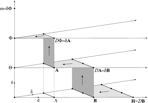
Figure 3: Derivation of ${\bf B}$, ${\bf A}$, $\Phi$ and $\omega$.

We always move towards the $r$ axis by inverting ${\cal D}$ up to gauge transformations, and to the top using $\delta$.

It is useful to evaluate the group cochains explicitly, so that all our relations read

$$\left\{\begin{array}[]{rcl}{\cal D}{\bf A}_{g}&=&g^{\ast}{\bf B}-{\bf B},\cr{\cal D}\Phi_{g,h}&=&g^{\ast}{\bf A}_{h}-{\bf A}_{gh}+{\bf A}_{g},\cr\omega_{g,h,k}&=&g^{\ast}\Phi_{h,k}\,\Phi^{-1}_{gh,k}\,\Phi_{g,hk}\,\Phi^{-1}_{g,h}.\end{array}\right.$$ (58)

The first equation means that ${\bf A}_{g}$ is a gauge transformation from ${\bf B}$ to $g^{\ast}{\bf B}$. Then, $(gh)^{\ast}{\bf B}$ can be obtained from ${\bf B}$ either by ${\bf A}_{gh}$, or by ${\bf A}_{g}+g^{\ast}{\bf A}_{h}$. Therefore, the two gauge transformations must be related by a residual gauge transformation $\Phi_{g,h}$. This is encoded in the second equation. The last equation arises from the two ways of combining two residual gauge transformations from ${\bf A}_{ghk}$ to ${\bf A}_{g}+h^{\ast}{\bf A}_{g}+(gh)^{\ast}{\bf A}_{k}$. Indeed, one can use either

$${\bf A}_{ghk}\xrightarrow{\Phi_{g,hk}}{\bf A}_{g}+g^{\ast}{\bf A}_{hk}\xrightarrow{g^{\ast}\Phi_{h,k}}{\bf A}_{g}+g^{\ast}{\bf A}_{h}+(gh)^{\ast}{\bf A}_{k},$$ (59)

or

$${\bf A}_{ghk}\xrightarrow{\Phi_{gh,k}}{\bf A}_{gh}+(gh)^{\ast}{\bf A}_{k}\xrightarrow{\Phi_{g,h}}{\bf A}_{g}+g^{\ast}{\bf A}_{h}+(gh)^{\ast}{\bf A}_{k}.$$ (60)

Since the two combinations of residual gauge transformations have the same action on ${\bf A}_{ghk}$, they differ by a constant which is $\omega_{g,h,k}$.

a)	b)	c)

Figure 4: Geometric illustration for group cochains.

In figure 4, vertices correspond to $B$-fields, arrows to gauge transformations ${\bf A}_{g}$, faces to residual gauge transformations $\Phi_{g,h}$ and $\omega_{g,h,k}$ to the tetrahedron obtained by gluing the two couples of triangles corresponding to (59) and (60).

Combining the gauge ambiguity on ${\bf B}$ as well as the ambiguities in the definition of ${\bf A}$ and $\Phi$, we obtain the following transformations

$$\left\{\begin{array}[]{lcl}{\bf B}&\rightarrow&{\bf B}+{\cal D}\Lambda\cr{\bf A}&\rightarrow&{\bf A}+\delta\Lambda+{\cal D}\Theta,\cr\Phi&\rightarrow&\Phi\,\delta\Theta\,\alpha,\cr\omega&\rightarrow&\omega\,\delta\alpha.\end{array}\right.$$ (61)

It is worthwhile to notice that $\omega$ is unaffected by the gauge transformations $\Lambda$ and $\Theta$, and is only modified through a group coboundary by $\alpha$. Upon evaluating the group indices, we get

$$\left\{\begin{array}[]{lcl}{\bf B}&\rightarrow&{\bf B}+{\cal D}\Lambda\cr{\bf A}_{g}&\rightarrow&{\bf A}_{g}+g^{\ast}\Lambda-\Lambda+{\cal D}\Theta_{g},\cr\Phi_{g,h}&\rightarrow&\Phi_{g,h}\;g^{\ast}\Theta_{h}\left(\Theta_{gh}\right)^{-1}\Theta_{g}\;\alpha_{g,h},\cr\omega_{g,h,k}&\rightarrow&\omega_{g,h,k}\;\alpha_{h,k}\left(\alpha_{gh,k}\right)^{-1}\alpha_{g,hk}\left(\alpha_{g,h}\right)^{-1}.\end{array}\right.$$ (62)

As a convention, we always assume that all the group cochains are normalized, i.e. they vanish whenever one of their arguments equals the identity of the group. This is always possible by exploiting the gauge freedom.

Besides, it is helpful to display C̆ech indices explicitly. We write ${\bf A}_{g}=\left(A_{g;\,i},f_{g;\,ij}\right)$ and $\Phi_{g,h}=\left(\phi_{g,h;\,i}\right)$, so that the system of equations (58) reads

$$\left\{\begin{array}[]{rcl}\mbox{d}A_{g;\,i}&=&g^{\ast}B_{i}-B_{i},\cr A_{g;\,j}-A_{g;\,i}-\mathrm{i}\,\mbox{d}\log f_{g;\,ij}&=&g^{\ast}B_{ij}-B_{ij},\cr(f_{g;\,jk})^{-1}f_{g;\,ik}(f_{g;\,ij})^{-1}&=&g^{\ast}f_{ijk}(f_{ijk})^{-1}\cr\mathrm{i}\,\mbox{d}\log\phi_{g,h;\,i}&=&g^{\ast}A_{h;\,i}-A_{gh;\,i}+A_{g;\,i},\cr\phi_{g,h;\,j}(\phi_{g,h;\,i})^{-1}&=&g^{\ast}f_{h;\,ij}(f_{gh;\,ij})^{-1}f_{g;\,ij},\cr\omega_{g,h,k}&=&g^{\ast}\phi_{h,k;\,i}\left(\phi_{gh,k;\,i}\right)^{-1}\phi_{g,hk;\,i}\left(\phi_{g,h;\,i}\right)^{-1}.\end{array}\right.$$ (63)

Up to a different sign convention, these are the equations derived by E. Sharpe in his analysis of discrete torsion [4], at the notable exception of the 3-cocycle $\omega$. As follows from our discussion, the triviality of $\omega$ cannot be obtained solely on the grounds of the invariance of $H$. However, it is an essential consistency condition in order to build an orbifold theory. We shall come back to this point at the end of section 4.3.

In the next section we will also have to use the equations obtained by displaying C̆ech indices for the gauge transformations,

$$\left\{\begin{array}[]{rclcl}A_{g;\,i}&\rightarrow&A_{g;\,i}+g^{\ast}\Lambda_{i}-\Lambda_{i}+\mathrm{i}\,\mbox{d}\log\theta_{g;\,i},\cr f_{g;\,ij}&\rightarrow&f_{g;\,ij}\;\theta_{g,j}(\theta_{g;\,i})^{-1}g^{\ast}\eta_{ij}(\eta_{ij})^{-1},\cr\phi_{g,h;\,i}&\rightarrow&\phi_{g,h;\,i}\;g^{\ast}\theta_{h;\,i}(\theta_{gh;\,i})^{-1}\theta_{g;\,i},\end{array}\right.$$ (64)

with $\Theta=\left(\theta_{g;\,i}\right)$. The transformation law of the components of ${\bf B}$ are identical to (49).

It is worthwhile to work out a simple example with globally defined fields. This requires the use of an infinite group and the simplest example is provided by the constant 3-form

$$H=\frac{1}{6}\,H_{\mu\nu\lambda}\,dx^{\mu}\wedge dx^{\nu}\wedge dx^{\lambda}$$ (65)

on ${\mathbb{R}}^{N}$ with the group $G={\mathbb{Z}}^{N}$. $B$, $A$ and $\phi$ are globally defined differential forms which are given, in suitable gauges, by

$$\left\{\begin{array}[]{rcl}B&=&\scriptsize{\frac{1}{6}}H_{\mu\nu\lambda}x^{\mu}\,dx^{\nu}\wedge dx^{\lambda}\cr A_{g}&=&\frac{1}{6}H_{\mu\nu\lambda}g^{\mu}x^{\nu}\,dx^{\lambda}\cr\phi_{g,h}&=&\exp\mathrm{i}\left\{\frac{1}{6}H_{\mu\nu\lambda}g^{\mu}h^{\nu}x^{\lambda}\right\}\cr\omega_{g,h,k}&=&\exp\mathrm{i}\left\{\frac{1}{6}H_{\mu\nu\lambda}g^{\mu}h^{\nu}k^{\lambda}\right\}\end{array}\right..$$ (66)

3.3 An interlude on the M-theory 3-form

We have worked out the explicit construction for a particle and a string, involving field strengths that are 2-forms and 3-forms. For higher dimensional extended objects, the same method applies. Starting with an $n$-form field strength which is invariant under the group $G$, we derive using the tricomplex a sequence of $k$-forms carrying $n-k-1$ group indices for $k=0,\dots,n-1$ and a constant group $n$-cocycle. This should be useful in the analysis of a supersymmetric theory like type IIA and IIB, whose spectrum involves forms of various degrees coupling to the branes. Analogously, this also applies to the M-theory 3-form $C$ and readily yields equations identical to those obtained in [11] and [12] in case of a trivial $4$-cocycle, as we now illustrate.

Let us start with an invariant globally defined closed 4-form $G$ that stands for the field strength. From $G$, we build

$${\bf G}=\left(G_{i},0,0,0,1\right)\in C_{0,4}^{\mathrm{tot}}.$$ (67)

It admits a set of locally defined potentials that we gather into

$${\bf C}=\left(C_{i},C_{ij},C_{ijk},f_{ijkl}\right)\in C_{0,3}^{\mathrm{tot}},$$ (68)

standing for the locally defined 3-form potentials $C_{i}$ and lower degree forms needed to glue them on non trivial intersections. The relation between the potentials and the field strength is summarized by

$${\cal D}{\bf C}={\bf G}.$$ (69)

There is a 2-form gauge invariance with gauge transformations $\Lambda\in C_{0,2}^{\mathrm{tot}}$,

$${\bf C}\rightarrow{\bf C}+{\cal D}\Lambda$$ (70)

as well as two levels of residual gauge transformations $\Xi\in C_{0,1}^{\mathrm{tot}}$ and $\chi\in C_{0,0}^{\mathrm{tot}}$ acting as

$$\Lambda\rightarrow\Lambda+{\cal D}\Xi\quad\mathrm{and}\quad\Xi\rightarrow\Xi+{\cal D}\chi.$$ (71)

In the mathematical language, the five equations obtained by expanding (69) define a 2-gerb with connection. Such an object is fundamental in M-theory since it couples to the worldvolume of a membrane in the same way that a $B$-field couples to a string.

Let us now assume that the field strength ${\bf G}$ is invariant under a group $G$ so that $\delta{\bf G}=0$. We further assume that ${\cal M}$ is such that the degree $k$ cohomology groups of the C̆ech-de Rham bicomplex are trivial for $k=1,2,3$. Thus, one can define ${\bf B}\in C_{1,2}^{\mathrm{tot}}$, ${\bf A}\in C_{2,1}^{\mathrm{tot}}$ and $\Phi\in C_{3,0}^{\mathrm{tot}}$ such that ${\cal D}{\bf B}=\delta{\bf C}$, ${\cal D}{\bf A}=\delta{\bf B}$ and ${\cal D}\Phi=\delta{\bf A}$ as well as $\omega=\delta\Phi$ which is a globally defined constant (${\cal D}\omega$=0) group 4-cocycle ($\delta\omega$=0). The rationale of this derivation is to move from ${\bf G}$ to the 4-cocycle $\omega$ in the tricomplex by inverting ${\cal D}$ up to gauge transformations to decrease the total C̆ech-de Rham degree and applying $\delta$ to get higher group cochains.

Upon displaying explicitly the group indices, these equations read

$$\left\{\begin{array}[]{rcl}{\cal D}{\bf B}_{g}&=&g^{\ast}{\bf C}-{\bf C},\cr{\cal D}{\bf A}_{g,h}&=&g^{\ast}{\bf B}_{h}-{\bf B}_{gh}+{\bf B}_{g},\cr{\cal D}\Phi_{g,h,k}&=&g^{\ast}{\bf A}_{h,k}-{\bf A}_{gh,k}+{\bf A}_{g,hk}-{\bf A}_{g,h},\cr\omega_{g,h,k,l}&=&g^{\ast}\Phi_{h,k,l}\left(\Phi_{gh,k,l}\right)^{-1}\Phi_{g,hk,l}\left(\Phi_{g,h,kl}\right)^{-1}\Phi_{g,h,k}.\end{array}\right.$$ (72)

If we assume that $\omega$ is trivial and display all C̆ech indices, then these equations are identical to the ones in [11] and [12]. Besides, there are various gauge ambiguities in the definitions of the fields ${\bf B}$, ${\bf A}$ and $\Phi$ as well as an extra constant phase in the definition of $\Phi$ alone. This is a group 3-cochain that changes $\omega$ by a coboundary. If we require that $\omega$ remains unchanged, it is a 3-cocycle which is identified in [11] with the M-theory analogue of discrete torsion.

4 Propagating string

4.1 Magnetic amplitudes and string wave functions

As for a particle, a closed string propagating on ${\cal M}$ in a background 3-form $H$ can be described in the functional integral approach by a magnetic amplitude. More precisely, the string propagator $K$ can be derived in perturbation theory from CFT as

$$K(Y,X)=\mathop{\int[D\varphi]}\limits_{\varphi(\partial{\cal S})=X^{\ast}\cup Y}\,e^{-S[\varphi]}{\cal A}[\varphi],$$ (73)

where $\varphi$ is a field from a two dimensional surface ${\cal S}$ into ${\cal M}$ whose boundary values coincide with the string initial and final positions $X$ and $Y$. Note that $X$ and $Y$ may both have several connected components and the topology of ${\cal S}$ encodes all the possible interactions. Besides, $K(Y,X)$ fulfills a set of axioms [13] and provides the evolution of the string wave function according to

$$\Psi(X)\rightarrow\Psi^{\prime}(Y)=\int[DX]\,K(Y,X)\Psi(X),$$ (74)

where $\Psi$ and $\Psi^{\prime}$ are functionals of the string’s embedding in space-time. In the following, we confine ourselves to the simplest topologies for ${\cal S}$: a cylinder (free string propagation) and a pair of pants (tree level decay of a string).

The magnetic amplitude ${\cal A}[\varphi]$ encodes all the couplings to the potentials of the external $H$-field and defines, together with $S[\varphi]$ a conformally invariant field theory on ${\cal S}$. Recall that the typical example we have in mind is the WZW model with ${\cal M}=\mathrm{SU(N)}$ and $H=\frac{k}{12\pi}\mathrm{Tr}\left(gdg^{-1}\right)^{3}$ the Maurer-Cartan 3-form. In this case, $H$ is closed but not exact and the explicit construction of the magnetic amplitudes requires the use of the locally defined potentials fulfilling $\eqref{gerb}$.

Let us now assume that a group $G$ acts on ${\cal M}$ and leaves $H$ as well as the kinetic term invariant. We aim at constructing magnetic amplitudes for some open strings in ${\cal M}$ that will define closed strings on the orbifold ${\cal M}/G$. These are the twisted sectors defined by strings that close up to an element of the group. More precisely, the space of strings with winding $w$ is

$${\cal C}_{w}=\left\{\,X_{w}:\,[0,2\pi]\rightarrow{\cal M}\quad\mbox{such that}\quad X(2\pi)=X(0)\cdot w\right\}.$$ (75)

For $w=e$ the identity of $G$, it corresponds to closed strings and one can glue together the endpoints of the segment to recover the circle $S^{1}$. In the general case, it is convenient to view strings in ${\cal C}_{w}$ as defined on a pointed circle, with boundary values differing by $w$, or equivalently, as strings defined on the universal cover ${\mathbb{R}}$ of $S^{1}$ fulfilling the quasi periodicity condition $X_{w}(\sigma+2n\pi)=X_{w}(\sigma)\cdot w^{n}$. In order to make the illustrations easier, we shall adopt the first point of view.

The simplest magnetic amplitude corresponds to a single free string of winding $w$ propagating between an initial position $X_{w}$ and a final one $Y_{w}$. We construct the amplitude using a slight modification of the powerful techniques introduced in [5] (with the sign conventions of [14]), in order to deal with the twisted sectors. Such an amplitude is associated to a map $\varphi$ from a cut cylinder ${\cal S}_{c}$ to ${\cal M}$, that interpolates between $X_{w}$ and $Y_{w}$ such that its boundary values along the cut differ by $w$.

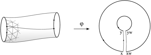
Figure 5: The cut of a cylinder.

Pick up a triangulation of the cut cylinder by 2-simplices $s_{\alpha}$, 1-simplices $l_{\beta}$ and vertices $v_{\gamma}$ such that there exists an assignment of open sets fulfilling $\varphi(s_{\alpha})\subset U_{i_{\alpha}}$, $\varphi(l_{\beta})\subset U_{i_{\beta}}$ and $\varphi(v_{\gamma})\in U_{i_{\gamma}}$. The triangulation also includes an indepedent triangulation of the cut by segments $l^{\prime}_{\beta^{\prime}}$ and vertices $v^{\prime}_{\gamma^{\prime}}$ which we assume to be identical on the two lips of the cut. That such a triangulation exists follows from the invariance property of the cover $\left\{U_{i}\right\}$.

We define the corresponding magnetic amplitude as

$${\cal A}[\varphi] = \prod\limits_{s_{\alpha}}\exp\mathrm{i}\left\{\int_{s_{\alpha}}\varphi^{\ast}B_{i_{\alpha}}\right\}\prod\limits_{\begin{subarray}{c}s_{\alpha}\\ l_{\beta}\subset\partial s_{\alpha}\end{subarray}}\exp\mathrm{i}\left\{\int_{l_{\beta}}\varphi^{\ast}B_{i_{\alpha}j_{\beta}}\right\}\prod\limits_{\begin{subarray}{c}s_{\alpha}\\ l_{\beta}\subset\partial s_{\alpha}\\ v_{\gamma}\in l_{\beta}\end{subarray}}\!\!\!\left\{\varphi^{\ast}f_{i_{\alpha}j_{\beta}k_{\gamma}}^{\epsilon_{\beta\gamma}}(v_{\gamma})\right\}$$ (76)

$$\times \prod\limits_{l^{\prime}_{\beta^{\prime}}}\exp\mathrm{i}\left\{\int_{l^{\prime}_{\beta^{\prime}}}\varphi^{\ast}A_{w;\,j_{\beta^{\prime}}}\right\}\prod\limits_{\begin{subarray}{c}l^{\prime}_{\beta^{\prime}}\\ v^{\prime}_{\gamma^{\prime}}\in\partial l^{\prime}_{\beta^{\prime}}\end{subarray}}\!\!\!\left\{\varphi^{\ast}f_{w;\,j_{\beta^{\prime}}k_{\gamma^{\prime}}}^{-\epsilon_{\beta^{\prime}\gamma^{\prime}}}(v^{\prime}_{\gamma^{\prime}})\right\}$$

The first line is identical to the contribution of closed strings in [5] and only involves the fields contained in ${\bf B}$. The second line is formally identical to the magnetic amplitude for a particle (6), but remember that $f_{w;ij}$ are not the transition functions of a line bundle because of the third equation in (63). This is reminiscent of the open string amplitudes [14], but ${\bf A}_{w}$ is not a new field of the theory since it is related to ${\bf B}$ by ${\cal D}{\bf A}_{w}=w^{\ast}{\bf B}-{\bf B}$. The rationale for this construction is to compensate all the defects of the open string amplitude on the cut by the contribution of the fields included in ${\bf A}_{g}$ integrated along the cut.

To compare the amplitudes associated to two different triangulations and assignments coinciding on the boundary strings $X_{w}$ and $Y_{w}$, one proceeds as follows. First, let us notice that it is sufficient to compare a triangulation to a finer one, i.e. a second triangulation that contains all the simplices of the first one. Then, we first compare all the terms arising form the 2-form $B_{i}$ in ${\bf B}=(B_{i},B_{ij},f_{ijk})$. Their integrals agree up to a discrepancy that only involves the 1-forms $B_{ij}$. The contribution of the latter also cancels with the scalars $f_{ijk}$, provided the corresponding edges do not meet the boundary. Next, compare all terms on the two lips of the cut, taking into account the contributions of the fields in ${\bf A}_{w}=(A_{w;\,i},f_{w;\,ij})$. Using (63), it turns out that all the terms on the upper lip cancel with all the terms on the lower lip, except on the boundary of the cut. This is a general rule: In proving any identity, one should always first compare the contribution of the top degree terms and add the corresponding discrepancy to the lower degree terms. Then, one repeats the procedure down to degree 0. Because of the high number of C̆ech indices involved in any non trivial computation, we do not display them here. Some typical examples are worked out in detail in [15].

Accordingly, the amplitude only depends on the fields ${\bf B}$ and ${\bf A}_{w}$ as well as on the triangulations and assignments $I$ and $J$ pertaining to the boundary strings $X_{w}$ and $Y_{w}$. Because the expression (76) is rather cumbersome to work with, we abbreviate it as

$${\cal A}_{JI}[\varphi]=\left[\mathrm{e}^{\mathrm{i}\int_{\Sigma}{\bf B}+\mathrm{i}\int_{x}^{y}{\bf A}_{w}}\right]_{JI},$$ (77)

where $x=X(0)$, $y=Y(0)$ and $\Sigma=\varphi({\cal S}_{c})$. It really means that one has to cut the cylinder, triangulate it and compute the amplitude as in (76). For topologically trivial $B$-fields, ${\bf B}$ and ${\bf A}$ can be identified with de Rham forms and (77) can be taken literally as the integrals of ${\bf B}$ over $\Sigma$ and of ${\bf A}_{w}$ over the cut joining $x$ to $y$. In any case, the contributions of ${\bf B}$ and ${\bf A}_{w}$ cannot be separated, only their combination is consistent.

The dependence of the amplitude on $I$ and $J$ is not very surprising. Indeed, recall that in the case of a particle, the amplitude is to be considered as a map from the fiber at $x$ to the fiber at $y$ of the bundle whose sections are the wave functions. Therefore, its definition involves a choice of open sets to cover $x$ and $y$. Something similar happens for strings. $I$ and $J$ are indices that label a covering of ${\cal C}_{w}$ by open sets $U_{I}$ and the string wave functions are sections of a bundle over ${\cal C}_{w}$, defined using transition functions $G_{IJ}$. The construction of the open sets covering ${\cal C}_{w}$ and of the transition functions also follows from [5].

If $I$ is a triangulation of the cut circle by segments $l_{\alpha}$ and vertices $v_{\beta}$ and an assignment of open sets $U_{i_{\alpha}}$ and $U_{j_{\beta}}$ that agree on the endpoints, we define

$$U_{I}=\left\{\,X\in{\cal C}_{w}\quad\mbox{such that}\quad X(l_{\alpha})\subset U_{i_{\alpha}}\quad\mbox{and}\quad X(v_{\beta})\in U_{i_{\beta}}\right\}.$$ (78)

Varying over all triangulations and assignments, these open sets cover ${\cal C}_{w}$.

Consider now an other triangulation $J$ of the cut circle by segments $l^{\prime}_{\alpha^{\prime}}$ and vertices $v^{\prime}_{\beta^{\prime}}$, and an assignment of open sets $U_{i^{\prime}_{\alpha^{\prime}}}$ and $U_{j^{\prime}_{\beta^{\prime}}}$. If $U_{I}\cap U_{J}$ is non empty, define a new triangulation of the intersection by segments $\bar{l}_{\bar{\alpha}}:=l_{\alpha}\cap l^{\prime}_{\alpha^{\prime}}$ and associated vertices $\bar{v}$. Further, set $i_{\bar{\alpha}}=i_{\alpha}$ and $i^{\prime}_{\bar{\alpha}}=i^{\prime}_{\alpha^{\prime}}$. For $\bar{v}$ set

$$j_{\bar{\beta}}=\left\{\begin{array}[]{c}j_{\beta}\\ i_{\alpha}\end{array}\quad\mathrm{if}\quad\begin{array}[]{c}\bar{v}=v_{\beta}\\ \bar{v}\in l_{\alpha}\end{array}\right.\quad,\quad j^{\prime}_{\bar{\beta}}=\left\{\begin{array}[]{c}j^{\prime}_{\beta^{\prime}}\\ i^{\prime}_{\alpha^{\prime}}\end{array}\quad\mathrm{if}\quad\begin{array}[]{c}\bar{v}=v^{\prime}_{\beta^{\prime}}\\ \bar{v}\in l^{\prime}_{\alpha^{\prime}}\end{array}\right..$$ (79)

Then, the transition functions $G_{IJ}$ are defined as

$$G_{IJ}(X)=\prod\limits_{\bar{l}}\exp\mathrm{i}\left\{\int_{\bar{l}}X^{\ast}\,B_{i_{\bar{\alpha}}i^{\prime}_{\bar{\alpha}}}\right\}\prod\limits_{\bar{v},\bar{l}|\bar{v}\in\partial\bar{l}}\left(\frac{X^{\ast}f_{j_{\bar{\beta}}j^{\prime}_{\bar{\beta}}i^{\prime}_{\bar{\alpha}}}(\bar{v})}{X^{\ast}f_{j_{\bar{\beta}}i_{\bar{\alpha}}i^{\prime}_{\bar{\alpha}}}(\bar{v})}\right)^{-\epsilon_{\bar{\beta}}}\times X^{\ast}f^{-1}_{w;\,j_{\beta_{0}}j^{\prime}_{\beta^{\prime}_{0}}}(0)$$ (80)

with $j_{\beta_{0}}$ and $j^{\prime}_{\beta^{\prime}_{0}}$ being the indices of open sets covering the cut and $\epsilon_{\bar{\beta}}$ takes values $-1$ if $\bar{v}$ is the first vertex of $\bar{l}$, and $+1$ if $\bar{v}$ is the second. When three opens sets intersect, the consistency condition for the transition functions read

$$G_{IK}(X)G_{KJ}(X)=G_{IJ}(X),$$ (81)

for $X\in U_{I}\cap U_{J}\cap U_{K}$. To check this identity, one has to use the three triangulations of the pointed circle and first compare the contributions of the 1-forms on both sides. They agree up to a boundary term, that is needed in order to cancel the discrepancy at the cut. The latter arises because $f_{w;\,ij}$ fails to be the transition function of a bundle (see equation (63)).

Accordingly, a line bundle can be constructed on ${\cal C}_{w}$ using these transition functions. The string wavefunction $\Psi$ is a section of this bundle defined locally in the chart $U_{I}$ by a complex valued function $\Psi_{I}$ that fulfills $\Psi_{I}=G_{IJ}\Psi_{J}$ on overlapping charts. We denote by ${\cal H}_{w}$ the space of sections of the line bundle over ${\cal C}_{w}$, it is the Hilbert space of strings with winding $w$. Note that when the winding is trivial ($w=e$), the previous construction reduces to the one presented in [5].

The dependence of the magnetic amplitudes on the covering and assignments pertaining to the endpoints is readily expressed using the transition functions. Indeed, if one trades $I$ and $J$ for $K$ and $L$, a simple calculation shows that

$$\left[\mathrm{e}^{\mathrm{i}\int_{\Sigma}{\bf B}+\mathrm{i}\int_{x}^{y}{\bf A}_{w}}\right]_{LK}=G_{LJ}(Y)\,\left[\mathrm{e}^{\mathrm{i}\int_{\Sigma}{\bf B}+\mathrm{i}\int_{x}^{y}{\bf A}_{w}}\right]_{JI}\,G_{IK}(X).\;$$ (82)

This is in agreement with its interpretation as an holonomy in the line bundle. Besides, the line bundle admits a connection that can be constructed along the lines of [5]. Roughly speaking, it corresponds to the infinitesimal version of the holonomy, but its precise mathematical definition is more involved because of the infinite dimensional nature of ${\cal C}_{w}$.

Consider now gauge transformations defined by $\Lambda=\left(\Lambda_{i},\eta_{ij}\right)$ and $\Theta_{g}=\left(\theta_{g;i}\right)$, whose explicit actions on the fields are given by (49) for $\Lambda$ and (64) for $\Theta$. This induces a change in the amplitude

$$\left[\mathrm{e}^{\mathrm{i}\int_{\Sigma}{\bf B}+\mathrm{i}\int_{x}^{y}{\bf A}_{w}}\right]_{JI}\rightarrow\left[\mathrm{e}^{\mathrm{i}\int_{\Sigma}\left({\bf B}+{\cal D}\Lambda\right)+\mathrm{i}\int_{x}^{y}\left({\bf A}_{w}+w^{\ast}\Lambda-\Lambda+{\cal D}\Theta_{w}\right)}\right]_{JI}.$$ (83)

Upon expressing everything using the triangulations and the explicit form of the gauge transformations, we see that there are cancelations that occur simplex by simplex in such a way that only boundary terms remain. The contribution along the cut of $\Lambda$ cancels with the lateral boundary of the worlsheet $\Sigma$, only the integrals of $\Lambda$ along the incoming and outcoming string remain, together with $\Theta_{w}$ and its inverse evaluated at $y$ and $x$. Therefore, the gauge transformed amplitude reads

$$\left[\Theta^{-1}_{w}(y)\mathrm{e}^{\mathrm{i}\int_{y}^{yw}\Lambda}\right]_{J}\left[\mathrm{e}^{\mathrm{i}\int_{\Sigma}{\bf B}+\mathrm{i}\int_{x}^{y}{\bf A}_{w}}\right]_{JI}\left[\Theta_{w}(x)\mathrm{e}^{-\mathrm{i}\int_{x}^{xw}\Lambda}\right]_{I},$$ (84)

where $\left[\cdots\right]_{I}$ always means that the expression inside the bracket is evaluated using the triangulation and assignment given by $I$.

For physics to remain invariant, the wave function has to be changed as

$$\Psi_{I}(X)\rightarrow\left[\Theta_{w}^{-1}(x)\mathrm{e}^{\mathrm{i}\int_{x}^{xw}\Lambda}\right]_{I}\Psi_{I}(X).$$ (85)

It is worthwhile to notice that in addition to the expected 1-form gauge transformation given by $\Lambda$, there is a new, winding dependent scalar gauge tranformation associated to $\Theta_{w}$. In the sequel, we shall refer to the latter as secondary gauge transformations.

The amplitude is also invariant under homotopic changes of the cut $c$ with endpoints fixed. To show this, we first extend the map $\varphi$ to the universal cover $\widetilde{\cal S}$ of the cylinder, taken as a strip, by quasi periodicity. Because we assume that the cover is invariant under the action of $G$, we can also extend it to a periodic triangulation of $\widetilde{\cal S}$. Any other cut $c^{\prime}$ defines another map $\varphi^{\prime}$ that coincides with $\varphi$ up to the action of elements of $G$ of the type $w^{n}$, $n\in{\mathbb{Z}}$, on $\varphi$ on various regions of $\widetilde{\cal S}$. Then we refine the triangulation used for $\varphi$ in order that it covers the new cut, leaving it unchanged on the boundary strings. Then, the new triangulation can also be used to compute the magnetic amplitude for $\varphi^{\prime}$ and the equality of the two amplitudes follows from repeated use of the relations (63) to compare the integrals over the regions differing by the action of $w^{n}$. This is illustrated in figure 7, where the change of the cut amounts to shifting the shaded area $\Sigma^{\prime\prime}$ by $w$, with $\Sigma^{\prime\prime}$ corresponding to the difference between the surfaces $\Sigma$ and $\Sigma^{\prime}$ provided by the maps $\varphi$ and $\varphi^{\prime}$.

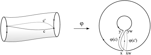
Figure 6: Homotopic change of the cut.

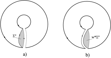
Figure 7: Difference between $\Sigma$ and $\Sigma^{\prime}$

Besides, the amplitude is invariant under diffeomorphisms of the cylinder that are connected to the identity and reduce to the identity on the boundary. Indeed, the latter simply reduce to a change of the triangulation followed by a change of variables in the associated integrals, as well as a smooth deformation of the cut. This is not the case for large diffeomorphisms because the latter induce a non homotopic change of the cut, as we shall see in section 5.2.

4.2 Stringy magnetic translations

At the classical level, the group $G$ transforms a string $X_{w}$ that starts at $x$ and ends at $x\!\cdot\!w$, into the string $X_{w}\!\cdot\!g$, starting at $x\!\cdot\!g$ and ending at $x\!\cdot\!wg=x\!\cdot\!g\,w^{g}$, with $w^{g}=g^{-1}wg$. Accordingly, $g$ changes the winding and defines a map from ${\cal C}_{w}$ to ${\cal C}_{w^{g}}$.

In analogy with the particle’s case, the stringy magnetic translation $T_{g}^{w}:\,{\cal H}_{w^{g}}\rightarrow{\cal H}_{w}$ realizing this operation at the quantum level is the pullback action on sections of the corresponding bundles, followed by a multiplication by a winding dependent phase factor,

$$\left[T_{g}^{w}\Psi\right]_{I}(X_{w})=\left[\Upsilon_{g}^{w}(X_{w})\right]_{I}\,\Psi_{I}(X_{w}\!\cdot\!g),$$ (86)

for any $X_{w}\in U_{I}\subset{\cal C}_{w}$. Because the open cover of ${\cal M}$ is invariant, we are allowed to use $U_{I}$ to cover ${\cal C}_{w^{g}}$, with the same triangulation and assignment. This can be summarized by the assertion that the collection of all $U_{I}$ forms an invariant cover of ${\cal C}=\cup_{w}{\cal C}_{w}$. Once we will have determined the covering dependent phase $\left[\Upsilon_{g}^{w}(X)\right]_{I}$, it will be necessary to show that all $\left[T_{g}^{w}\Psi\right]_{I}$ can be glued together to form a section over ${\cal C}_{w}$ that belongs to ${\cal H}_{w}$. Accordingly, $T_{g}^{w}$ will be a linear map from ${\cal H}_{w^{g}}$ into ${\cal H}_{w}$.

As for the particle, we determine the unknown phase by requiring that $T_{g}^{w}$ commutes with string propagation. To obtain a sufficient condition ensuring this commutation, let us perform a heuristic analysis, similar to the path integral derivation in section 2.2. The propagation process of a string of winding $w$ is expressed as

$$\Psi_{w}(X)\rightarrow\Psi^{\prime}_{w}(Y)=\int[DX]\,K_{w}(Y,X)\Psi_{w}(X),$$ (87)

where we have omitted the index $I$ for clarity but have displayed the windings. In terms of matrix elements, the commutation relation $T_{g}^{w}K_{w^{g}}=K_{w}T_{g}^{w}$ reads

$$\Upsilon_{g}^{w}(Y)K_{w^{g}}(Y\!\cdot\!g,X\!\cdot\!g)=K_{w}(Y,X)\Upsilon_{g}^{w}(X),$$ (88)

which is analogous to (18).

Assuming that all terms in the path integral (73) but the magnetic amplitudes are genuinely invariant under the action of $G$ (as is the case for WZW models), it is sufficient to analyse the behavior of the latter under the action of $G$. By equating the magnetic contribution of $\varphi$ and $\varphi\cdot g$ in the path integral on both sides of (88),

$$\left[\Upsilon_{g}^{w}(Y)\right]_{J}{\cal A}_{JI}[\varphi\!\cdot\!g]={\cal A}_{JI}[\varphi]\left[\Upsilon_{g}^{w}(X)\right]_{I},$$ (89)

we get a sufficient condition for the commutation to hold.

The expression of the magnetic amplitude for $\varphi\!\cdot\!g$ follows from the results of the previous section,

$${\cal A}_{JI}[\varphi\!\cdot\!g]=\left[\mathrm{e}^{\mathrm{i}\int_{\Sigma}g^{\ast}{\bf B}+\mathrm{i}\int_{x}^{y}g^{\ast}{\bf A}_{w^{g}}}\right]_{JI}.$$ (90)

Recall that $g^{\ast}{\bf B}$ and $g^{\ast}{\bf A}_{w^{g}}$ are related to ${\bf B}$ and ${\bf A}_{w^{g}}$ by (58), which implies

$$\left\{\begin{array}[]{rcl}g^{\ast}{\bf B}&=&{\bf B}+{\cal D}{\bf A}_{g},\\ g^{\ast}{\bf A}_{w^{g}}&=&{\bf A}_{wg}-{\bf A}_{g}+{\cal D}\Phi_{g,w^{g}}.\end{array}\right.$$ (91)

To eliminate the unwanted ${\bf A}_{w^{g}}$, it is useful to introduce

$$\Gamma_{w,g}=\Phi_{g,w^{g}}\left(\Phi_{w,g}\right)^{-1},$$ (92)

which fulfills

$${\cal D}\Gamma_{w,g}+w^{\ast}{\bf A}_{g}-{\bf A}_{g}=g^{\ast}{\bf A}_{w^{g}}-{\bf A}_{w}.$$ (93)

Therefore, the ratio of the two amplitudes reads

$$\frac{{\cal A}_{JI}[\varphi\!\cdot\!g]}{{\cal A}_{JI}[\varphi]}=\left[\mathrm{e}^{\mathrm{i}\int_{\Sigma}{\cal D}{\bf A}_{g}+\mathrm{i}\int_{x}^{y}\left({\cal D}\Gamma_{w,g}+w^{\ast}{\bf A}_{g}-{\bf A}_{g}\right)}\right]_{JI}.$$ (94)

This expression can be calculated using a triangulation and an assignment of open sets, coinciding with $I$ and $J$ on the boundary and expressing ${\bf A}_{g}$ and $\Gamma_{w,g}$ as C̆ech cochains. When performing this computation, lots of cancelations occur and only boundary terms remain. The final result is

$$\frac{{\cal A}_{JI}[\varphi\!\cdot\!g]}{{\cal A}_{JI}[\varphi]}=\left[\Gamma_{w,g}^{-1}(y)\mathrm{e}^{\mathrm{i}\int_{y}^{yw}{\bf A}_{g}}\right]_{J}\left[\Gamma_{w,g}(x)\mathrm{e}^{-\mathrm{i}\int_{x}^{xw}{\bf A}_{g}}\right]_{I}.$$ (95)

Because of its cumbersome nature, the computation cannot be displayed here, but it is instructive to check it for topologically trivial fields. In this case, ${\bf A}_{g}$ is an ordinary 1-form and ${\cal D}$ is the de Rham differential, so that Stockes theorem yields

$$\int_{\Sigma}\mbox{d}A_{g}=\int_{\partial\Sigma}A_{g}.$$ (96)

The integral over the boundary is expressed as

$$\int_{\partial\Sigma}A_{g}=\int_{y}^{yw}A_{g}-\int_{x}^{xw}A_{g}+\int_{x}^{y}\left(A_{g}-w^{\ast}A_{g}\right).$$ (97)

The integral over the cut cancels with the corresponding term in

$$\int_{x}^{y}\left(\mathrm{i}\mbox{d}\log\Gamma_{w,g}+w^{\ast}A_{g}-A_{g}\right),$$ (98)

so that we are left with boundary terms only, in accordance with (95).

Turning back to the general case, we compare (95) with (89) and set

$$\left[\Upsilon_{g}^{w}(X)\right]_{I}=\left[\Gamma_{w,g}(x)\,\mathrm{e}^{-\mathrm{i}\int_{x}^{xw}{\bf A}_{g}}\right]_{I}.$$ (99)

Accordingly, the stringy magnetic translations are defined as

$$\left[T_{g}^{w}\Psi\right]_{I}(X)=\left[\Gamma_{w,g}(x)\,\mathrm{e}^{-\mathrm{i}\int_{x}^{xw}{\bf A}_{g}}\right]_{I}\,\Psi_{I}(X\!\cdot\!g),$$ (100)

and the discussion preceding (89) ensures that it commutes with propagation.

Strictly speaking, we have defined $T_{g}^{w}$ only for wave functions defined on local charts. To have operators defined between ${\cal H}_{w^{g}}$ and ${\cal H}_{w}$, we have to check that all $\left[T_{g}^{w}\Psi\right]_{I}$ for various $I$ can be glued into a global section on ${\cal C}_{w}$. This follows from the relation

$$\frac{G_{IJ}(X\!\cdot\!g)}{G_{IJ}(X)}=\frac{\left[\Gamma_{w,g}(x)\,\mathrm{e}^{-\mathrm{i}\int_{x}^{xw}{\bf A}_{g}}\right]_{I}}{\left[\Gamma_{w,g}(x)\,\mathrm{e}^{-\mathrm{i}\int_{x}^{xw}{\bf A}_{g}}\right]_{J}},$$ (101)

that is obtained from the explicit form of $G_{IJ}$ given in (80).

There is a very simple illustration of the action of a stringy magnetic translation. Consider the process in which a single string with trivial winding $w=e$ is created out of the vacuum. The corresponding magnetic amplitude is

$${\cal A}_{I}[\varphi]=\left[\mathrm{e}^{\mathrm{i}\int_{\Sigma}{\bf B}}\right]_{I},$$ (102)

where $\Sigma=\varphi({\cal S})$ is a cap as in figure 8.

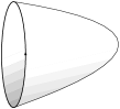
Figure 8: A cap.

This amplitude is to be inserted in a path integral (73),

$$\Psi_{I}(X)=\mathop{\int[D\varphi]}\limits_{\varphi(\partial{\cal S})=X}\,e^{-S[\varphi]}{\cal A}_{I}[\varphi],$$ (103)

and yields a wave function for a string of trivial winding, which is obviously invariant under $G$.

4.3 Multiplication law

In the particle’s case, we have seen that magnetic translations only form a projective representation of $G$. In order to check if something similar happens for a string, let us compare $T_{g}^{w}T_{h}^{w^{g}}$ with $T_{gh}^{w}$. On the left hand side, starting with $\Psi\in{\cal H}_{w^{gh}}$, we first act with $T_{h}^{w^{g}}$

$$\Psi^{\prime}_{I}(X)=\left[T_{h}^{w^{g}}\Psi\right]_{I}(X)=\left[\Gamma_{w^{g},h}(x)\,\mathrm{e}^{-\mathrm{i}\int_{x}^{xw^{g}}{\bf A}_{h}}\right]_{I}\,\Psi_{I}(X\!\cdot\!h),\quad\mathrm{with}\,X\in{\cal C}_{w^{g}}.$$ (104)

Then, we further act on $\Psi^{\prime}\in{\cal H}_{w^{g}}$ with $T_{g}^{w}$,

$$\left[T_{g}^{w}\Psi^{\prime}\right]_{I}(X)=\left[\Gamma_{w,g}(x)\,\mathrm{e}^{-\mathrm{i}\int_{x}^{xw}{\bf A}_{g}}\right]_{I}\,\Psi^{\prime}_{I}(X\!\cdot\!g),\quad\mathrm{with}\,X\in{\cal C}_{w}.$$ (105)

Replacing $\Psi^{\prime}$ by its expression, we arrive at

$$\left[T_{g}^{w}T_{h}^{w^{g}}\Psi\right]_{I}(X)=\left[\Gamma_{w,g}(x)\,g^{\ast}\Gamma_{w^{g},h}(x)\,\mathrm{e}^{-\mathrm{i}\int_{x}^{xw}\left({\bf A}_{g}+g^{\ast}{\bf A}_{h}\right)}\right]_{I}\,\Psi_{I}(X\!\cdot\!gh),\quad\mathrm{with}\,X\in{\cal C}_{w},$$ (106)

where we have used the pullback operation of $g$ to trade the integral of ${\bf A}_{h}$ over the string $X\!\cdot\!g$ for the integral of $g^{\ast}{\bf A}_{h}$ over $X$.

On the other hand side, we act directly with $T_{gh}^{w}$ to get

$$\left[T_{gh}^{w}\Psi\right]_{I}(X)=\left[\Gamma_{w,gh}(x)\,\mathrm{e}^{-\mathrm{i}\int_{x}^{xw}{\bf A}_{gh}}\right]_{I}\,\Psi_{I}(X\!\cdot\!gh).$$ (107)

Thus, there is a phase mismatch between $T_{gh}^{w}$ and $T_{g}^{w}T_{h}^{w^{g}}$,

$$T_{g}^{w}T_{h}^{w^{g}}=\frac{\left[\Gamma_{w,g}(x)\,g^{\ast}\Gamma_{w^{g},h}(x)\,\mathrm{e}^{-\mathrm{i}\int_{x}^{xw}\left({\bf A}_{g}+g^{\ast}{\bf A}_{h}\right)}\right]_{I}}{\left[\Gamma_{w,gh}(x)\,\mathrm{e}^{-\mathrm{i}\int_{x}^{xw}{\bf A}_{gh}}\right]_{I}}\,T_{gh}^{w}.$$ (108)

Using ${\cal D}\Phi_{g,h}=g^{\ast}{\bf A}_{h}-{\bf A}_{gh}+{\bf A}_{g}$, cancelations similar to the ones in (95) occur in the explicit evaluation using C̆ech cochains. The result can be expressed solely with $\Phi$:

$$\frac{\left[\Gamma_{w,g}(x)\,g^{\ast}\Gamma_{w^{g},h}(x)\,\mathrm{e}^{\mathrm{i}\int_{x}^{xw}\left({\bf A}_{g}+g^{\ast}{\bf A}_{h}\right)}\right]_{I}}{\left[\Gamma_{w,gh}(x)\,\mathrm{e}^{\mathrm{i}\int_{x}^{xw}{\bf A}_{gh}}\right]_{I}}=\left[\frac{\Phi_{g,w^{g}}\,g^{\ast}\Phi_{h,w^{gh}}\,\Phi_{w,gh}\,w^{\ast}\Phi_{g,h}}{\Phi_{w,g}\,g^{\ast}\Phi_{w^{g},h}\,\Phi_{gh,w^{gh}}\,\Phi_{g,h}}(x)\right]_{I}.$$ (109)

After repeated use of $\omega=\delta\Phi$, the previous expression simplifies to

$$\left[\frac{\Phi_{g,w^{g}}\,g^{\ast}\Phi_{h,w^{gh}}\,\Phi_{w,gh}\,w^{\ast}\Phi_{g,h}}{\Phi_{w,g}\,g^{\ast}\Phi_{w^{g},h}\,\Phi_{gh,w^{gh}}\,\Phi_{g,h}}(x)\right]_{I}=\frac{\omega_{w,g,h}\,\omega_{g,h,w^{gh}}}{\omega_{g,w^{g},h}}.$$ (110)

Because ${\cal D}\omega=0$, $\omega$ is globally defined (i.e. it does not depend on the open set in which it has been computed) and constant. This is why we dropped the $I$ and $X$ in the notation. The occurrence of this combination of the 3-cocycle $\omega$ corresponds to chopping the prism spanned by $w$, $w^{g}$ and $w^{gh}$ into three tetrahedra, as can be seen in figure 9.

Figure 9: The phase of the product in terms of tetrahedra.

Finally, the product law reads

$$T_{g}^{w}T^{v}_{h}=\delta_{v,w^{g}}\,\frac{\omega_{w,g,h}\,\omega_{g,h,w^{gh}}}{\omega_{g,w^{g},h}}\,T_{gh}^{w},$$ (111)

where we have defined the product as zero when the windings do not match. This is exactly the multiplication of the quasi-quantum group $D_{w}[G]$ introduced in [3]. Thus, as operators on the full Hilbert space ${\cal H}=\oplus_{w}{\cal H}_{w}$, the $T_{g}^{w}$ generate the quasi-quantum group $D_{w}[G]$. Though a 3-cocycle usually indicates a breakdown of an associativity law, the product of three stringy magnetic translations remains associative, since they are operators in the Hilbert space. This last property can be checked directly using the cocycle properties of $\omega$. Nevertheless, we shall see in the next section that there is failure of associativity when considering the interaction of three strings.

The expression of the phase factor appearing in the multiplication law (111) in terms of the 3-cocycle $\omega$ is easily interpreted using a transgression map similar to the one introduced in [17]. Let us denote by $(C,\delta)$ the standard group cohomology complex with values in $U(1)$ and by $(\widetilde{C},\tilde{\delta})$ a new complex whose cochains are group cochains with values in $U(1)$-valued functions over $G$. For any $n$-cochain in $\widetilde{C}^{n}$ defined by the function $w\mapsto\widetilde{c}_{g_{1},\dots,g_{n}}(w)$, we define the twisted coboundary as

$$(\tilde{\delta}\tilde{c})_{g_{0},\dots,g_{n}}(w)=\tilde{c}_{g_{1},\dots,g_{n}}(w^{g_{0}})\times\prod_{k=1}^{n}\left(\tilde{c}_{g_{0},\dots,g_{k-1}g_{k},\dots,g_{n}}(w)\right)^{(-1)^{k}}\times\left(\tilde{c}_{g_{0},\dots,g_{n-1}}(w)\right)^{(-1)^{n+1}}.$$ (112)

The transgression map ${\cal T}$ takes an $(n+1)$-cochain $c_{g_{1},\dots,g_{n+1}}\in C^{n+1}$ to an $n$-cochain in $\widetilde{C}$ by

$$\left[{\cal T}c\right]_{g_{1},\dots,g_{n}}(w)=\prod_{i=0}^{n}\left(c_{g_{1},\dots,g_{i},w^{g_{1}\dots g_{i}},g_{i+1},\dots,g_{n}}\right)^{(-1)^{n-i}}.$$ (113)

For cocycles $\beta$, $\alpha$ and $\omega$ of orders 1,2 and 3, we have

$$\left[{\cal T}\beta\right](w)=\beta_{w},\quad\left[{\cal T}\alpha\right]_{g}(w)=\frac{\alpha_{g,w^{g}}}{\alpha_{w,g}},\quad\left[{\cal T}\omega\right]_{g,h}(w)=\frac{\omega_{w,g,h}\omega_{g,h,w^{gh}}}{\omega_{g,w^{g},h}}.$$ (114)

The transgression map induces a morphism of complexes since it fulfills ${\cal T}\circ\delta=\tilde{\delta}\circ{\cal T}$. Therefore, the image of an $(n+1)$-cocycle in $C$ is an $n$-cocycle in $\tilde{C}$. In particular, the 3-cocycle $\omega$ is transgressed into a 2-cocycle on functions of the winding, which allows to interpret the product law (111) of stringy magnetic translations as a projective representation.

Let us close this section by a brief comment on the orbifold construction. Starting with a string theory on ${\cal M}$, the latter consists in two steps. First, one introduces the twisted sectors, that form the Hilbert space ${\cal H}$. Then, one projects the Hilbert space onto the subspace made out of vectors that are invariant (up to a phase) under the action of $G$. In case the 3-cocycle $\omega$ is non trivial, there are no invariant states with a non trivial winding. This is similar to the particle’s case, as we have seen in section 2. If there is a phase mismatch between $T_{g}T_{h}$ and $T_{gh}$, no non trivial invariant states can be constructed in ${\cal H}$, unless $\omega$ is cohomologically trivial in the sense of [18]. Indeed, the representations of $D_{\omega}[G]$ can be understood as direct sums of projective representations in each conjugacy classes [19]. In the orbifold string theory, these conjugacy classes define the sectors and for cohomologically trivial $\omega$ the phases of the operators $T_{g}^{w}$ may be adjusted in such a way that there is no phase in the multiplication law. However, as we shall see in the last section, global anomalies remain when $\omega\neq 1$. Therefore, the triviality of $\omega$ appears as an additional consistency obstruction for the orbifold theory, as already noticed in [4], but cannot be derived solely from the invariance of the 3-form $H$ under the group.

On the geometrical side, $\omega$ can be considered as an obstruction to pushing forward the gerb on ${\cal M}$ defined by $\eqref{gerb}$ to a gerb on ${\cal M}/G$ when the action of $G$ is free. This interpretation is in accordance with the results obtained in [16] in case of simply connected Lie groups quotiented by finite subgroups.

Even if we assume that $\omega=1$, it is in general impossible to gauge away the extra phases $\Upsilon_{g}^{w}$ simultaneously for all $g\in G$. Indeed, this would require $\Upsilon_{g}^{w}$ to be independent of $g$, which implies that so do ${\bf A}_{g}$ and $\Gamma_{w}^{g}$. This is in general not the case, as can be checked on the simple example given by a constant $H$ in (66).

5 Interacting strings

5.1 Quasi Hopf structure from interactions

The cornerstone of the subsequent derivation of the quasi-quantum group structure of the algebra generated by the stringy magnetic translations resides in the geometrical nature of the interactions of strings. Indeed, let us consider a process in which $m$ incoming strings scatter to produce $n$ outgoing ones, which gives rise to an operator $K^{m\rightarrow n}$ from ${\cal H}^{\otimes m}$ to ${\cal H}^{\otimes n}$. In the wave function approach adopted here, the matrix elements of $K^{m\rightarrow n}$ can be derived from a two dimensional field theory as

$$K^{m\rightarrow n}(Y,X)=\mathop{\int[D\varphi]}\limits_{\varphi(\partial{\cal S})=X^{*}\cup Y}\,\mathrm{e}^{-S[\varphi]},$$ (115)

where $\varphi:{\cal S}\rightarrow{\cal M}$ is the conformal field describing the embedding of the strings into space-time. Of course, one has to further integrate over the moduli of the Riemann surface ${\cal S}$ and sum over all possible genera. The surface ${\cal S}$ has a boundary made of $m+n$ circles, the n circles $Y=(Y_{1},\dots,Y_{n})$ whose orientation agrees with that of $\varphi(\partial{\cal S})$ correspond to the outgoing strings while the $m$ others $X=(X_{1},\dots,X_{m})$ are the incoming ones.

In the previous sections, we have already dealt with simple examples restricted to free strings: $K^{1\rightarrow 1}$ and $K^{0\rightarrow 1}$, describing respectively the propagation and the creation of a single string out of the vacuum. In the sequel, we shall deal with interacting strings, restricting ourselves to the simplest processes. The first example we treat in detail is the tree level contribution to the decay process $K^{1\rightarrow 2}$ involving pairs of pants. This allows us to derive the coproduct of $D_{\omega}[G]$ from the requirement of the commutativity of $K^{1\rightarrow 2}$ with stringy magnetic translations. Then, we show that the defining relations for the antipode of $D_{\omega}[G]$ arises from the orientation reversing operation that relates $K^{0\rightarrow 2}$ and $K^{1\rightarrow 1}$. Other features of the quasi-quantum group $D_{\omega}[G]$ have natural counterparts in the theory of interacting strings. We illustrate this for the associator, the braiding and the invariance under Drinfel’d twists, respectively related to the failure of the associativity of the tensor product of several strings, the exchange of two strings and discrete torsion.

Derivation of the coproduct

The most basic interaction is given by the tree level decay of a string of winding $vw$ into a string of winding $v$ and another one of winding $w$. The matrix element $K^{1\rightarrow 2}(Y\cup Z,X)$ is associated to the pants ${\cal S}$ depicted in figure 10.

Figure 10: Basic interaction associated to a pair of pants.

To construct the corresponding magnetic amplitude for a map $\varphi$ such that $\varphi(\partial{\cal S})=X^{*}\cup Y\cup Z$, one has to cut the pants in order to obtain a simply connected surface. Then, the magnetic amplitude reads

$${\cal A}_{JK,I}[\varphi]=\left[\mathrm{e}^{\mathrm{i}\int_{\Sigma}{\bf B}+\mathrm{i}\int_{x}^{t}{\bf A}_{vw}+\mathrm{i}\int_{t}^{y}{\bf A}_{v}+\mathrm{i}\int_{tv}^{z}{\bf A}_{w}}\;\Phi_{v,w}^{-1}(t)\right]_{JK,I},$$ (116)

where $I$ is used to cover the incoming string while $J$ and $K$ label the covers of the two outgoing strings. The insertion of $\Phi^{-1}_{v,w}$ is necessary to maintain invariance under the secondary gauge transformations of ${\bf A}$ and $\Phi$ given by (62). Indeed, 1-form gauge transformations of ${\bf B}$ and ${\bf A}$ cancel together at the boundary $\partial\Sigma$, except on the boundary strings as is expected. The secondary gauge transformation induced by $\Theta\in C^{\mathrm{tot}}_{1,0}$ also has boundary terms on the strings as expected by (83), and an extra contribution at the point $t$ where the three cuts meet. If we denote by $U_{l}$ the open set used to cover the point $t$, a secondary gauge transformation yields $[\Theta^{-1}_{vw}(x)]_{l}$ along the cut joining $x$ to $t$ and $[\Theta_{v}(t)\Theta_{w}(t\!\cdot\!v)]_{l}$ along the two other cuts leaving $t$. The net result is $[v^{\ast}\Theta_{w}\Theta^{-1}_{vw}\Theta_{v}]_{l}$, which is canceled by the secondary gauge transformation of $[\Phi^{-1}_{v,w}(t)]$ given in (62). Obviously, if we consider the reversed process in which two strings join, one has to insert $\Phi_{v,w}$. It is interesting to note that a similar phase factor has been encountered in the context of toroidally compactified closed string field theory [20]. Whereas our phase factor is a 2-cochain on the windings, their phase factor is a 2-cocycle on the momenta. This is equivalent, since T-duality exchanges windings and momenta, and their cocycle condition simply stipulates the triviality of $\omega$.

The amplitude is independent of the homotopy class of the three cuts and under diffeomorphisms connected to the identity that act trivially on the boundary strings, as one may check using the same techniques as for the free string propagator. Besides, using the relation ${{\cal D}}\Phi_{v,w}=v^{\ast}{\bf A}_{w}-{\bf A}_{vw}+{\bf A}_{v}$, one can also move the point $t$ along the cut, leaving the amplitude unchanged.

This amplitude contributes to the process describing the tree level decay ${\cal H}_{vw}\rightarrow{\cal H}_{v}\otimes{\cal H}_{w}$. We expect that the corresponding operator $K_{v,w}$ (the upper index $\cdot^{1\to 2}$ has been omitted for convenience) commutes with the action of $G$, but the latter may be defined on the tensor product ${\cal H}_{v}\otimes{\cal H}_{w}$ only up to an additional phase. Again, we determine this phase by an heuristic analysis, focusing on the magnetic amplitude only.

The magnetic amplitude is to be inserted into the path integral for the evolution operator $K_{v,w}$ encoding the decay process ${\cal H}_{vw}\rightarrow{\cal H}_{v}{\otimes}{\cal H}_{w}$,

$$K_{v,w}\left(Y\cup Z,X\right)=\mathop{\int[D\varphi]}\limits_{\varphi(\partial{\cal S})=X^{\ast}\cup Y\cup Z}\,\mathrm{e}^{-S[\varphi]}{\cal A}[\varphi],$$ (117)

where $X$, $Y$ and $Z$ are three strings of respective windings $vw$, $v$ and $w$. In this heuristic analysis we have omitted indices relative to the coverings for clarity.

To determine the possible extra phase in the tensor product, we compare the operators $K_{v,w}T_{g}^{vw}$ and $\left(T_{g}^{v}\otimes T_{g}^{w}\right)K_{v^{g},w^{g}}$. At the level of the kernels, we have to compare

$$K_{v,w}(Y\cup Z,X)\Upsilon_{g}^{vw}(X)$$ (118)

and

$$\Upsilon_{g}^{v}(Y)\Upsilon_{g}^{w}(Z)K_{v^{g},w^{g}}(Y\!\cdot\!g\cup Z\!\cdot\!g,X\!\cdot\!g),$$ (119)

with $\Upsilon_{g}^{w}$ the phase defining the stringy magnetic translation. Let us proceed as we did for single string propagations in the last section by comparing the magnetic amplitudes. ${\cal A}_{JK,I}[\varphi]$ enters into $K_{v,w}(Y\cup Z,X)$ whereas ${\cal A}_{JK,I}[\varphi\!\cdot\!g]$ is the corresponding term in $K_{v^{g},w^{g}}(Y\!\cdot\!g\cup Z\!\cdot\!g,X\!\cdot\!g)$.

To begin with, the translated amplitude involving strings of windings $v^{g}$, $w^{g}$ and $(vw)^{g}$ reads

$${\cal A}_{JK,I}[\varphi\!\cdot\!g]=\left[\mathrm{e}^{\mathrm{i}\int_{\Sigma}g^{\ast}{\bf B}+\mathrm{i}\int_{x}^{t}g^{\ast}{\bf A}_{(vw)^{g}}+\mathrm{i}\int_{t}^{y}g^{\ast}{\bf A}_{v^{g}}+\mathrm{i}\int_{tv}^{z}g^{\ast}{\bf A}_{w^{g}}}\;g^{\ast}\Phi^{-1}_{v^{g},w^{g}}(t)\right]_{JK,I}.$$ (120)

After some manipulations using the relations (63), the ratio can be expressed as

$$\frac{{\cal A}_{JK,I}[\varphi\!\cdot\!g]}{{\cal A}_{JK,I}[\varphi]}=\left[\frac{\Gamma^{-1}_{v,g}(y)\,\mathrm{e}^{\mathrm{i}\int_{y}^{yv}{\bf A}_{g}}\;\Gamma^{-1}_{w,g}(z)\,\mathrm{e}^{\mathrm{i}\int_{z}^{zw}{\bf A}_{g}}}{\Gamma^{-1}_{vw,g}(x)\,\mathrm{e}^{\mathrm{i}\int_{x}^{xvw}{\bf A}_{g}}}\times\frac{\Phi_{v,w}\,\Gamma_{v,g}\,v^{\ast}\Gamma_{w,g}}{g^{\ast}\Phi_{v^{g},w^{g}}\,\Gamma_{vw,g}}(t)\right]_{JK,I}.$$ (121)

The first ratio in the bracket can be written as

$$\frac{\left[\Gamma^{-1}_{v,g}(y)\,\mathrm{e}^{\mathrm{i}\int_{y}^{yv}{\bf A}_{g}}\right]_{J}\;\left[\Gamma^{-1}_{w,g}(z)\,\mathrm{e}^{\mathrm{i}\int_{z}^{zw}{\bf A}_{g}}\right]_{K}}{\left[\Gamma^{-1}_{vw,g}(x)\,\mathrm{e}^{\mathrm{i}\int_{x}^{xvw}{\bf A}_{g}}\right]_{I}}=\frac{\left[\Upsilon_{g}^{vw}(X)\right]_{I}}{\left[\Upsilon_{g}^{v}(Y)\right]_{J}\,\left[\Upsilon_{g}^{w}(Z)\right]_{K}}.$$ (122)

It is exactly what one expects from acting with $T_{g}^{vw}$ on the incoming string and $T_{g}^{v}{\otimes}T_{g}^{w}$ on the two outgoing ones, so that it cancels when acting with the stringy magnetic translations.

The second one can be expressed using the 3-cocycle $\omega$ as

$$\left[\frac{g^{\ast}\Phi_{v^{g},w^{g}}\,\Gamma_{vw,g}}{\Phi_{v,w}\,\Gamma_{v,g}\,v^{\ast}\Gamma_{w,g}}(t)\right]_{JK,I}=\frac{\omega_{v,w,g}\,\omega_{g,v^{g},w^{g}}}{\omega_{v,g,w^{g}}}.$$ (123)

Because its expression only involves $\omega$, it is globally defined and constant.

Therefore, the action of $G$ on the tensor product ${\cal H}_{v^{g}}\otimes{\cal H}_{w^{g}}$ must be defined as

$$\frac{\omega_{v,w,g}\,\omega_{g,v^{g},w^{g}}}{\omega_{v,g,w^{g}}}\,\left(T_{g}^{v}\otimes T_{g}^{w}\right).$$ (124)

This is nothing but the phase appearing in the coproduct $\Delta:\,D_{\omega}[G]\rightarrow D_{\omega}[G]\otimes D_{\omega}[G]$ of the quasi-quantum group, defined in [3] as

$$\Delta(T_{g}^{u})=\mathop{\sum}\limits_{vw=u}\,\frac{\omega_{v,w,g}\,\omega_{g,v^{g},w^{g}}}{\omega_{v,g,w^{g}}}\,T_{g}^{v}{\otimes}T_{g}^{w}.$$ (125)

The occurrence of the coproduct in the action on the tensor product is natural in the theory of quasi Hopf algebras (see appendix). Indeed, given two representations $\rho_{1}$ and $\rho_{2}$ of $D_{\omega}[G]$, a new one can be build as

$$\left(\rho_{1}\otimes\rho_{2}\right)\circ\Delta.$$ (126)

This is exactly what happens for strings in a background 3-form $H$: the representation acting on ${\cal H}_{v}\otimes{\cal H}_{w}$ is nothing but the tensor product of the representations on ${\cal H}_{v}$ and on ${\cal H}_{w}$, but with the tensor product defined using the coproduct rule (126).

As for the phase appearing in the product, the phase of the coproduct can be understood in terms of a prism, representing the translation by $g$ of a string of winding $vw$ decomposed into a string of winding $v$ followed by a string of winding $w$. The decomposition of the prism into the three tetrahedra components is depicted in figure 11.

Figure 11: The phase of the coproduct in terms of tetrahedra.

This coproduct is only quasi-coassociative,

$$\left(\mathrm{id}{\otimes}\Delta\right)\circ\Delta=\Omega\big{(}\left(\Delta{\otimes}\mathrm{id}\right)\circ\Delta\big{)}\Omega^{-1},$$ (127)

where $\Omega$ is the Drinfel’d associator, related to the 3-cocycle $\omega$ by

$$\Omega=\mathop{\sum}\limits_{u,v,w}\omega_{u,v,w}^{-1}\,T_{e}^{u}{\otimes}T_{e}^{v}{\otimes}T_{e}^{w}.$$ (128)

Together with the antipode and the braiding to be defined in subsequent sections, the quasi-quantum group $D_{\omega}$ turns out to be a quasi-triangular quasi Hopf algebra.

In accordance with the general theory of quasi Hopf algebras, let us note that $D_{\omega}[G]$ also comes equipped with a counit defined as $\epsilon(T_{g}^{w})=\delta_{w,e}$ [3].

In the case of globally defined fields given by (66) in the case $G={\mathbb{Z}}^{N}$, the product is

$$T_{g}^{w}T_{h}^{v}=\delta_{v,w}\;\mathrm{e}^{\,\frac{\mathrm{i}}{6}H_{\mu\nu\lambda}w^{\mu}g^{\nu}h^{\lambda}}\;T_{gh}^{w}$$ (129)

and the coproduct

$$\Delta\left(T_{g}^{w}\right)=\mathop{\sum}\limits_{uv=w}\,\mathrm{e}^{\,\frac{\mathrm{i}}{6}H_{\mu\nu\lambda}g^{\mu}u^{\nu}v^{\lambda}}\;T_{g}^{u}{\otimes}T_{g}^{v}.$$ (130)

As an algebra, it is nothing but a direct sum of noncommutative tori with winding dependent phases inserted in the multiplication law of the generators. The coproduct mixes different windings and turns out to be coassociative because the associator is central. From a pure mathematical viewpoint, this is rather interesting because it is known that noncommutative tori are not Hopf algebras. The Hopf algebra structure can only be obtained by taking into account all the windings. However, the associator does not drop from the quasi Yang-Baxter equation (184) and the quasi triangular structure only holds in the sense of quasi Hopf algebras.

As an aside, let us note that the product and the coproduct of $D_{\omega}[G]$ admit a cohomological interpretation very similar to the transgression already introduced in (114). Indeed, the consistency of the quasi Hopf algebra structure implies that the phases appearing in the product (111)

$${\cal P}^{g,h}_{w}=\frac{\omega_{w,g,h}\,\omega_{g,h,w^{gh}}}{\omega_{g,w^{g},h}},$$ (131)

and coproduct (125)

$${\cal Q}^{g}_{v,w}=\frac{\omega_{v,w,g}\,\omega_{g,v^{g},w^{g}}}{\omega_{v,g,w^{g}}}$$ (132)

obey the following equations

$$\left\{\begin{array}[]{rcl}{\cal P}_{u}^{g,h}\,{\cal P}_{u}^{gh,k}&=&{\cal P}_{u}^{g,hk}\,{\cal P}_{u^{g}}^{h,k},\cr{\cal P}_{u}^{g,h}\,{\cal P}_{v}^{g,h}\,{\cal Q}^{g}_{u,v}\,{\cal Q}^{h}_{u^{g},v^{g}}&=&{\cal P}_{uv}^{g,h}\,{\cal Q}^{gh}_{u,v},\cr{\cal Q}_{u,v}^{g}\,{\cal Q}_{uv,w}^{g}\,\omega_{u^{g},v^{g},w^{g}}&=&{\cal Q}_{v,w}^{g}\,{\cal Q}_{u,vw}^{g}\,\omega_{u,v,w}.\end{array}\right.$$ (133)

The first equation expresses the associativity of the product, the second one the compatibility of the product and the coproduct and the last one the quasi-coassociativity of the coproduct.

Using the group coboundary $\delta$ for the windings $u,v,w,\dots$ and the twisted group coboundary $\tilde{\delta}$ (generalizing the one introduced in $\eqref{twisted}$) for $g,h,k,\dots$, with an extra action by conjugation on the windings for its first factor, these equations read

$$\left\{\begin{array}[]{rcl}(\tilde{\delta}{\cal P})_{u}^{g,h,k}&=&1,\cr(\tilde{\delta}{\cal Q})_{u,v}^{g,h}\,(\delta{\cal P})_{u,v}^{g,h}&=&1,\cr(\delta{\cal Q})_{u,v,w}^{g}\,\left((\tilde{\delta}{\omega})_{u,v,w}^{g}\right)^{-1}&=&1.\end{array}\right.$$ (134)

Together with $(\delta\omega)_{u,v,w}=1$, these equations simply stipulate that $({\cal P}^{g,h}_{u},{\cal Q}_{u,v}^{g},\omega_{u,v,w})$ is a 2-cocycle in a bicomplex constructed out of $\delta$ and $\tilde{\delta}$.

Antipode

In the general formula (5.1) encoding the scattering process of several strings, whether a string is incoming or outgoing depends on its orientation with respect to that of the surface ${\cal S}$ involved in the matrix element. However, a given ${\cal S}$ can contribute to various processes differing solely by the choice of the incoming and outgoing nature of the strings among the circles defined by $\partial{\cal S}$.

This suggests the existence of an operator ${\Pi}$ from ${\cal H}$ to its dual that changes an outgoing string to an incoming one. At the wave function level, if $\Psi\in{\cal H}_{w}$, then we define $\Pi\Psi\in\left({{\cal H}_{w^{-1}}}\right)^{\ast}$ by

$$\left[\Pi\Psi(X^{\ast})\right]_{I^{\ast}}=\left[\Phi_{w,w^{-1}}(x)\right]_{I}\left[\Psi(X)\right]_{I},$$ (135)

where $X^{\ast}\in{\cal C}_{w^{-1}}$ denotes the string with orientation reversed and $I^{\ast}$ is the triangulation and assignment with order reversed. $\Pi\Psi$ is a section of the dual bundle defined by the transition functions $G_{IJ}^{\ast}=G_{IJ}^{-1}$ and with gauge transformations and holonomies along cylinders defined by the opposite phases. As for the pair of pants amplitude in the last section, the inclusion of the winding dependent extra phase $\Phi_{w,w^{-1}}$ is dictated by the requirement of invariance under secondary gauge transformations. In geometrical terms, $\Pi$ is a line bundle isomorphism induces by the orientation reversing.

For general Hopf algebras (see for instance [7]), the antipode allows to define the dual of a given representation. In our context, the antipode ensures the compatibility of the quasi-quantum group action on the string states with the orientation reversing operation. Indeed, if $\Psi\in{\cal H}_{w}$ and $\Psi^{\prime}\in{\cal H}_{(w^{-1})^{g}}$, then we have

$$\left[\Pi\left(T_{g}^{w}\Psi\right)(X^{\ast})\right]_{I^{\ast}}\Psi^{\prime}_{I}(X^{\ast})=\left[\Pi\Psi(X^{\ast}\!\cdot\!g)\right]_{I^{\ast}}\left[S(T_{g}^{w})\Psi^{\prime}(X^{\ast}\!\cdot\!g)\right]_{I}$$ (136)

for any string $X^{\ast}\in{\cal C}_{w^{-1}}$, with

$$S(T_{g}^{w})=\frac{\omega_{g,(w^{-1})^{g},g^{-1}}}{\omega_{w^{-1},g,g^{-1}}\,\omega_{g,g^{-1},w^{-1}}}\,\frac{\omega_{w,g,(w^{-1})^{g}}}{\omega_{w,w^{-1},g}\,\omega_{g,w^{g},(w^{-1})^{g}}}\,T_{g^{-1}}^{(w^{-1})^{g}}$$ (137)

the antipode of the quasi-quantum group (see [3]). Note that the first phase factor is nothing but the inverse of the phase appearing in the product $T^{w^{-1}}_{g}T^{(w^{-1})^{g}}_{g^{-1}}$ (see (111)) while the second phase factor is the inverse of the one appearing in the coproduct for a translation of $g$ of two strings of windings $w$ and $w^{-1}$. Note that (136) can be used to derive the extra phase in (137).

$S$ fulfills all the requirements imposed on the antipode of a quasi-Hopf algebra (see appendix), with trivial $\alpha$ and

$$\beta=\sum_{w}\omega_{w,w^{-1},w}\,T_{g}^{w}.$$ (138)

Besides, its square obeys

$$S^{2}(a)=\beta^{-1}a\beta$$ (139)

for any $a\in D_{\omega}[G]$, as shown in [18].

To illustrate the previous construction on a simple example, let us consider a two string state $K^{0\rightarrow 2}$ created out of the vacuum. Reversing the orientation of the first string, we recover the single string propagator

$$(\Pi\otimes\mbox{id})K^{0\rightarrow 2}=K^{1\rightarrow 1}.$$ (140)

At the level of matrix elements, this equation reads

$$\Phi_{w,w^{-1}}(x)K^{0\rightarrow 2}_{w,w^{-1}}(X,Y)=K^{1\rightarrow 1}_{w^{-1}}(Y,X^{\ast}).$$ (141)

The simplest topology that contributes to these processes is that of a cylinder, whose magnetic amplitude for $K^{1\rightarrow 1}$ is given in (77). The magnetic contribution of the same cylinder to $K^{0\rightarrow 2}$ is obtained by gluing a cap to a pair of pants. Using the homotopy invariance, it is readily seen to be in accordance with (141), the extra factor $\Phi_{w,w^{-1}}(x)$ of the orientation reversing operation being canceled by the inverse factor due to the interaction. The commutation of the action of the quasi quantum group with $K^{0\rightarrow 2}$ reads

$$\Delta(a)K^{0\rightarrow 2}=\epsilon(a)K^{0\rightarrow 2}.$$ (142)

Reversing the orientation of the first string yields, using Sweedler’s notation for the coproduct (see appendix),

$$(\Pi\otimes\mbox{id})\left((a_{(1)}\otimes a_{(2)})K^{0\rightarrow 2}\right)=a_{(2)}K^{1\rightarrow 1}S\left(a_{(1)}\right).$$ (143)

To derive the last equation, we have used (136) that states that the action of $a\in D_{\omega}[G]$ on an outgoing state becomes, after orientation reversing, the dual action of $S(a)$ on the corresponding incoming state. Then, (142) translates into

$$a_{(2)}S\left(a_{(1)}\right)=\epsilon(a).$$ (144)

The latter follows from one of the defining relations of the antipode

$$a_{(1)}\beta S(a_{(2)})=\epsilon(a)\beta,$$ (145)

after acting with $S$ and using (139) and its antimorphism property $S(ab)=S(b)S(a)$, valid for arbitrary quasi-Hopf algebras.

Associator on string states

The quasi-quantum group $D_{\omega}[G]$ is a quasi-triangular quasi Hopf algebra. We refer to [6] for some general background on quasi Hopf algebras and their applications. We have collected in the appendix a few results that are useful in our context. The category of representations of such an algebra forms a quasi-tensor (or braided monoidal) category which is a far reaching generalization of the category of representation of a group. Roughly speaking, this is a category where tensor products are defined, with an associativity law that holds only up to isomorphism, as well as the exchange of the factors in the tensor products, which is implemented using the braid group instead of the symmetric group. This setting, termed quasi Hopf symmetry, has been proposed in [21] as a natural framework that is versatile enough to encompass all possible symmetries in physics. For example, a quasi Hopf symmetry based on $D_{\omega}[G]$ appears in the study of topological excitations coupled to non abelian Chern-Simons theory in 2+1 dimensions [22].

Let us now illustrate the quasi-associativity (associativity up to isomorphims) of the tensor product in the context of interacting strings. As already mentioned, the tensor product of two representations $\rho_{1}$ and $\rho_{2}$ of $D_{\omega}[G]$ has to be defined using the coproduct rule (126). Consider now the tensor product of three representations $\rho_{1}$, $\rho_{2}$ and $\rho_{3}$. Because the coproduct is only quasi coassociative (see (127)), one has to distinguish between the two parenthesings of the tensor products $\rho_{1}\otimes(\rho_{2}\otimes\rho_{3})$ and $(\rho_{1}{\otimes}\rho_{2}){\otimes}\rho_{3}$, these two representations being intertwined by the image of $\Omega$.

The failure of associativity is very natural from the point of view of the magnetic amplitudes. Consider the process in which one string of winding $uvw$ decays into three of windings $u$, $v$ and $w$. Such a process arises from the composition of two pairs of pants in two different ways (see figure 12).

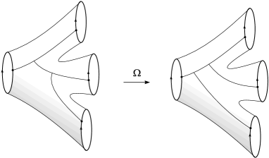
Figure 12: Two different cuts related by the associator.

To compare the two amplitudes, it is again useful to apply the relation ${\cal D}\Phi_{g,h}=g^{\ast}{\bf A}_{h}-{\bf A}_{gh}+{\bf A}_{g}$ in such a way that the two branching points of the cut come together. However, they cannot pass through each other and they always remain in the same order. We have depicted the fine structure of the branching point for the $1\to 3$ decay in figure 13.

$\leftrightarrow$

Figure 13: The fine structure of the branching point, with all $\Phi^{-1}$’s evaluated at $x$.

The two amplitudes coincide except that the branching yields $\left[\Phi_{uv,w}^{-1}\Phi_{u,v}^{-1}\right]_{i}$ for the first and $\left[u^{\ast}\Phi_{v,w}^{-1}\Phi_{u,vw}^{-1}\right]_{i}$ for the second, with $i$ being the index of the open set used to cover the branching point. Thus, the second amplitude simply differs from the first one by the phase factor $\omega_{u,v,w}$. This is in perfect agreement with the quasi Hopf point of view, since the pattern of splittings implies that the first process reads

$${\cal H}_{uvw}\rightarrow{\cal H}_{uv}{\otimes}{\cal H}_{w}\rightarrow({\cal H}_{u}{\otimes}{\cal H}_{v}){\otimes}{\cal H}_{w},$$ (146)

whereas the second is

$${\cal H}_{uvw}\rightarrow{\cal H}_{u}{\otimes}{\cal H}_{vw}\rightarrow{\cal H}_{u}{\otimes}({\cal H}_{v}{\otimes}{\cal H}_{w}).$$ (147)

The two processes end in two different tensor products, differing only by their parenthesings. This statement is illustrated in figure 14, where we indicated the different parenthesings on the Hilbert spaces by the dashed ellipses encircling the corresponding states.

$\stackrel{{\scriptstyle\Omega}}{{\longrightarrow}}$

Figure 14: Quasi-associativity on the states.

It is compatible with the action of magnetic translations, which differ by the same phase for the two parenthesings.

The same result holds for more general amplitudes: the pattern of interactions involved selects the parenthesing of the Hilbert spaces appearing on the boundary. This is particularly clear if we consider processes in which one string can decay into $n$ strings. The branching of the cut yields a tree that encodes all the information on the parenthesis to be used. The choice made for intermediate states is irrelevant since changing their parenthesing always produce two phases that cancel. Any change in the parenthesing can be implemented by successive applications of the associator that moves branches of the tree from one side of the corresponding branching point to the other side. Using MacLane’s coherence theorem [6], the cocycle condition on $\omega$ implies that any sequence of associators between two fixed parenthesing always yields the same phase.

As already noticed for invariant states, the physical requirement of the consistency of the orbifold forces $\omega$ to be trivial, so that these complications do not arise in practice. In this case, the quasi-quantum group reduces to the quantum double of the group $G$.

5.2 Tree level amplitudes

Consider now all the tree level amplitudes describing the decay of one string into $n$ others. From now on, we always assume $\omega$ to be trivial, unless otherwise stated, so that there is no need to keep track of the parenthesings. Any tree level amplitude can be obtained by gluing cylinders and pants together. The resulting surface has a mapping class group (i.e. those diffeomorphisms that are not connected to the identity) generated by the Dehn twists of the cylinder and the braidings of the pants. All these operators can be constructed using the quasi-quantum group $D_{\omega}[G]$.

Dehn twist of the cylinder

The magnetic translations allow us to understand the transformation of the cylinder amplitude under large diffeomorphisms. The cylinder amplitude reads

$${\cal A}_{JI}[\varphi]=\left[\mathrm{e}^{\mathrm{i}\int_{\Sigma}{\bf B}+\mathrm{i}\int_{x}^{y}{\bf A}_{w}}\right]_{JI}.$$ (148)

If we act with a Dehn twist on the cylinder, then the cut $c$ is changed into $c^{\prime}$ which induces a corresponding change $\varphi\rightarrow\varphi^{\prime}$. In the target space ${\cal M}$, the transformation yields a new worldsheet $\Sigma^{\prime}$ and the image of the new cut joins $x$ to $y\!\cdot\!w$, as can be seen in figure 15.

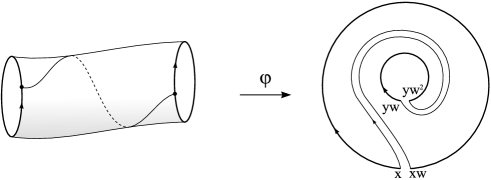
Figure 15: The Dehn twist of the cylinder.

Therefore, we get an other amplitude ${\cal A}_{JI}[\varphi^{\prime}]$ and the ratio of the two amplitudes turns out to be

$$\frac{{\cal A}_{JI}[\varphi^{\prime}]}{{\cal A}_{JI}[\varphi]}=\left[\mathrm{e}^{\mathrm{i}\int_{\Sigma^{\prime\prime}}\left(w^{\ast}{\bf B}-{\bf B}\right)+\mathrm{i}\int_{x}^{yw}{\bf A}_{w}-\mathrm{i}\int_{x}^{y}{\bf A}_{w}}\right]_{JI}.$$ (149)

This follows from the fact that $\Sigma$ and $\Sigma^{\prime}$ only differ by the shaded surface $\Sigma^{\prime\prime}$ (see figure 16), whose contribution is lifted by $w$ in ${\cal A}_{JI}[\varphi^{\prime}]$ with respect to its contribution to ${\cal A}_{JI}[\varphi]$. After using $w^{\ast}{\bf B}={\bf B}+{\cal D}{\bf A}_{w}$ in the explicit expression of the ratio, only boundary terms remain. Two of them cancel with the integrals along the cut and we are left with

$$\frac{{\cal A}_{JI}[\varphi^{\prime}]}{{\cal A}_{JI}[\varphi]}=\left[\mathrm{e}^{\mathrm{i}\int_{y}^{yw}{\bf A}_{w}}\right]_{J}.$$ (150)

Recall the translation by $w$ of a string $Y$ with winding $w$,

$$\left[T_{w}^{w}\Psi\right]_{J}(Y)=\left[\mathrm{e}^{-\mathrm{i}\int_{y}^{yw}{\bf A}_{w}}\right]_{J}\Psi_{J}(Y).$$ (151)

Thus, the action of the Dehn twist simply amounts to translating the outgoing string by its own winding. Starting with the twisted cylinder one constructs the twisted propagator $K^{\prime}$ and the comparison of the magnetic amplitudes for $\varphi$ and $\varphi^{\prime}$ shows that $T_{w}^{w}K_{w}^{{}^{\prime}}=K_{w}$. Because of the commutation of $T_{w}^{w}$ and $K_{w}$, the twist can as well be implemented on the incoming string.

Figure 16: The surface $\Sigma^{\prime\prime}$.

Braiding of the pair of pants

Consider now the large diffeomorphism of the pant that induces a braiding of the cut as in figure 17.

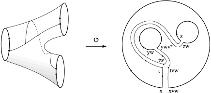
Figure 17: The braiding.

The braiding induces the change $\varphi\rightarrow\varphi^{\prime}$ associated to the new amplitude

$${\cal A}_{KJ,I}[\varphi^{\prime}]=\left[\mathrm{e}^{\mathrm{i}\int_{\Sigma^{\prime}}{\bf B}+\mathrm{i}\int_{x}^{t}{\bf A}_{vw}+\mathrm{i}\int_{tw}^{yw}{\bf A}_{v^{w}}+\mathrm{i}\int_{t}^{z}{\bf A}_{w}}\;\Phi^{-1}_{w,v^{w}}(t)\right]_{KJ,I}$$ (152)

where the line integrals involve the cuts in figure 17. The new amplitude ${\cal A}_{KJ,I}[\varphi^{\prime}]$ differs from the old one ${\cal A}_{JK,I}[\varphi]$ given in (116) by the ordering of the windings ($(v,w)\rightarrow(w,v^{w})$) and by the shaded surface (see figure 18) which is removed from $\Sigma$, lifted by $w$ and reinserted into $\Sigma$ to form $\Sigma^{\prime}$.

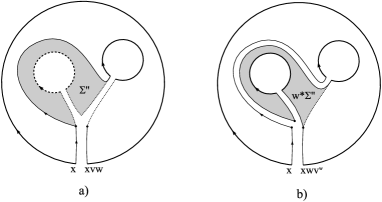
Figure 18: The surface $\Sigma^{\prime\prime}$ and its lift by $w$.

Thus, the ratio of the two amplitudes is

$$\frac{{\cal A}_{KJ,I}[\varphi^{\prime}]}{{\cal A}_{JK,I}[\varphi]}=\left[\Gamma_{v,w}^{-1}(y)\;\mathrm{e}^{\mathrm{i}\int_{y}^{yv}{\bf A}_{w}}\right]_{J}.$$ (153)

This matches exactly the phase that appears in the operator $T_{w}^{v}$. Therefore, the braiding of the pants induces a change of the magnetic amplitude ${\cal A}_{JK,I}[\varphi]\rightarrow{\cal A}_{KJ,I}[\varphi^{\prime}]$ that corresponds to the braid group action derived from the general theory of quasi-triangular quasi Hopf algebras (see appendix). Indeed, the quasi-quantum group $D_{\omega}[G]$ is equipped with an ${\cal R}$-matrix defined by

$${\cal R}=\mathop{\sum}\limits_{v,w}T_{e}^{v}{\otimes}T_{v}^{w}.$$ (154)

When acting on a tensor product of two states, it simply leaves the first string invariant and translates the second by the winding of the first. The corresponding action of the braid group with two strands $B_{2}$ is defined by its generator $\sigma=\tau\circ{\cal R}$, where $\tau$ is the flip. If we restrict ourselves to strings with fixed windings, this induces a map $\sigma_{v,w}:\,{\cal H}_{w}\otimes{\cal H}_{v^{w}}\rightarrow{\cal H}_{v}\otimes{\cal H}_{w}$ defined by $\sigma_{v,w}=\tau\circ(1\otimes T_{w}^{v})$. Then, the same reasoning as for the twist of the cylinder applies: The braiding yields another pant ${\cal S^{\prime}}$ whose field $\varphi^{\prime}$ defines a propagator $K^{\prime}$ related to $K$ by $\sigma_{v,w}K^{\prime}_{w,v^{w}}=K_{v,w}$.

Note that thanks to the quasi-triangularity condition

$$\tau\circ\Delta={\cal R}\,\Delta{\cal R}^{-1},$$ (155)

the braid group action commutes with the stringy magnetic translations, provided the latter act on tensor products using the coproduct rule.

When more than two factors are involved (recall that, for the moment, we take $\omega$ to be trivial, i.e. the Drinfel’d associator is also trivial), the exchange of the factors is governed by the braid group with $N$ strands $B_{N}$. The latter is generated by the operators $\sigma_{i}=\tau\circ{\cal R}$ that exchange the two adjacent factors located at the $i^{\mathrm{th}}$ and $(i+1)^{\mathrm{th}}$ place in the tensor product. The defining relations of $B_{N}$, i.e.

$$\left\{\begin{array}[]{rclr}\sigma_{i}\sigma_{j}&=&\sigma_{j}\sigma_{i}&\mbox{if}\quad|i-j|>1\cr\sigma_{i}\sigma_{i+1}\sigma_{i}&=&\sigma_{i+1}\sigma_{i}\sigma_{i+1}&\mbox{otherwise},\end{array}\right.$$ (156)

hold thanks to the Yang-Baxter equation (see appendix),

$${\cal R}_{12}{\cal R}_{13}{\cal R}_{23}={\cal R}_{23}{\cal R}_{13}{\cal R}_{12}.$$ (157)

Together with the Dehn twists of the cylinder, the braid group $B_{N}$ generates the mapping class group of the pants with one incoming and $N$ outgoing strings.

Braided operad

The tree level amplitudes corresponding to the decay of a single string into $N$ others are conveniently visualized as follows.

• Draw a large cut circle that stands for the incoming string.

• Draw $N$ smaller circles inside the larger one that represent the outgoing strings.

• Relate the endpoints of the incoming string to those of the outgoing ones by a tree, allowing for twists around the circles and braids around two neighbouring circles.

An amplitude for a process $1\rightarrow N$ can be glued with $N$ amplitudes for $1\rightarrow n_{N}$ so that the result is an amplitude pertaining to the process $1\rightarrow\sum_{i=1}^{N}n_{i}$. In figure 19, we give a simple example of gluing three amplitudes into the corresponding slots of a first one.

Figure 19: The braided operad structure of tree level amplitudes.

More generally, denoting by $\Delta_{n}$ the set of amplitudes with $n$ outgoing strings, the gluings define composition laws

$$\gamma_{N}:\,\Delta_{N}\times\Delta_{n_{1}}\times\cdots\times\Delta_{n_{N}}\rightarrow\Delta_{n_{1}+\cdots+n_{N}}.$$ (158)

The sets $\Delta_{n}$ carry an obvious representation of the braid group $B_{n}$, with generators $\sigma_{i}$ acting in the same manner as for the pair of pants. The action is compatible with the gluing, in the sense that braiding before gluing is equivalent to braiding after gluing. Altogether, this means that the decaying amplitudes form a braided operad [23].

In all the preceeding discussion we have assumed that the 3-cocycle $\omega$ is trivial. If this is not the case, the braid group action still makes sense, but some care is required because of the lack of associativity of the tensor product. For the action of $B_{N}$ defined using its generators $\sigma_{i}$ one has to make a repeated use of the associator to make sure that the parenthesings do not seperate the two factors being exchanged. Therefore, when composing $\sigma_{i}$ and $\sigma_{j}$, one has to insert suitable representations of the associator (see appendix). The defining relations of the braid group (156) then follow from the quasi Yang-Baxter equation (184), which is a modification of the Yang-Baxter equation (157) in order to take into account the Drinfel’d associator.

5.3 Loop amplitudes

The simplest loop amplitude to consider is the torus, that can be obtained from the cylinder by gluing the two boundaries using a stringy magnetic translation as depicted in figure 20.

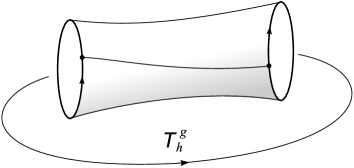
Figure 20: Obtaining a torus amplitude from a cylinder.

The amplitude reads

$${\cal A}[\varphi]=\left[\mathrm{e}^{\mathrm{i}\int_{\Sigma}{\bf B}+\int_{x}^{x\cdot h}{\bf A}_{g}-\mathrm{i}\int_{x}^{x\cdot g}{\bf A}_{h}}\,\Gamma_{g,h}(x)\right],$$ (159)

where $g$ and $h$ are two mutually commuting elements of $G$. It is obtained from the cylinder amplitude of a propagating string of winding $g$ by adding the extra phase corresponding to the translation by $h$ of a string of winding $g$, and should be though of as being inserted into a functional integral contributing to the trace of $(T_{h}^{g})K_{g}$, which is further summed over $g$ and $h$ to provide the torus partition function.

Because there is no boundary, it does not depend at all on the triangulation used in its computation. Nevertheless, we write it into brackets to remember that its actual definition relies on some triangulation. Besides, it is invariant under homotopic changes of the cut, diffeomorphisms connected to the identity and gauge transformations. These properties are valid whether $\omega$ is trivial or not.

However, when $\omega$ is non trivial, the torus amplitude is plagued by global anomalies: it receives extra phases under global translations and large diffeomorphisms of the torus. Under a global translation $\varphi\rightarrow\varphi\!\cdot\!k$, the amplitude changes according to

$${\cal A}[\varphi\!\cdot\!k]=\frac{\omega_{k,h^{k},g^{k}}\,\omega_{g,k,h^{k}}\,\omega_{h,g,k}}{\omega_{k,g^{k},h^{k}}\,\omega_{g,h,k}\,\omega_{h,k,g^{k}}}\,{\cal A}[\varphi].$$ (160)

Using the relation (111) and its geometrical intepretation given in figure 9, this combination of 3-cocycles can be understood as a way of chopping the parallelepiped build out of $g$, $h$ and $k$ into six tetrathedra. When all three group elements commute, this matches (up to a global sign) the topological action for a 3-torus in finite group topological field theory [24].

The group of large diffeomorphisms of the torus is generated by the modular transformations $T$ and $S$ that induce the following changes in the group elements along the cut,

$$\begin{array}[]{ccc}T:\quad\left\{\begin{array}[]{lcl}g&\rightarrow&gh\\ h&\rightarrow&h\end{array}\right.&&S:\quad\left\{\begin{array}[]{lcl}g&\rightarrow&h^{-1}\\ h&\rightarrow&g\end{array}\right.\end{array}.$$ (161)

Again, the amplitude changes by extra phases depending on the 3-cocycle $\omega$. Indeed, $T$ acts as

$${\cal A}[\varphi]\rightarrow{\cal A}[T\varphi]=\omega_{h,g,h}\,{\cal A}[\varphi]$$ (162)

and $S$ as

$${\cal A}[\varphi]\rightarrow{\cal A}[S\varphi]=\frac{\omega_{h,g,h^{-1}}}{\omega_{h,h^{-1},g}\,\omega_{g,h,h^{-1}}}\,{\cal A}[\varphi].$$ (163)

This behaviour of the torus amplitude and of all the previous tree level amplitudes under global translations and large diffeomorphisms yields relations that are very similar to the ones in [25], derived in the context of CFT. In fact, this last paper deals with algebraic properties of the conformal blocks in an orbifold theory with group $G$. It is rather amazing that the formulae pertaining to the transformation of conformal blocks are so close to the ones derived here for magnetic amplitudes, especially because our derivation relies solely on the geometry of the Kalb-Ramond field and does not refer to CFT.

More generally, we expect all loop amplitudes to be flawed by these global anomalies under translation and global diffeomorphisms. This is due to the insertion of the gauge fields ${\bf A}_{g}$ and $\Phi_{g,h}$ along the internal cuts, which is required by gauge invariance. Any global change induces a change of these gauge fields which is only partially compensated along the two boundaries of the cut. This is another clue that the orbifold theory is consistent only for trivial $\omega$.

If we assume that $\omega$ is trivial, then one can construct the magnetic amplitude for an arbitrary surface as follows. At the tree level, we construct the amplitude by gluing together cylinders and pairs of pants as given in (76) and (116). For the latter it is crucial to insert a factor of $\Phi^{-1}_{v,w}$ when a string of winding $vw$ splits into two strings of windings $v$ and $w$ and $\Phi_{v,w}$ when they join. Loop amplitudes are obtained by further gluing together some incoming and outgoing strings using the operators $T_{g}^{w}$. At the level of magnetic amplitudes, this translates into insertions of the phases $\Upsilon_{g}^{w}$ when a string of winding $w$ is glued with its lift by $g$. Then, the triviality of $\omega$ ensures that the amplitude is independent of the patterns of joining and splitting, as well as under global translations and large diffeomorphisms.

5.4 Relation to discrete torsion

Let us now assume that $\omega$ is trivial, so that the orbifold exists, and come to grips with discrete torsion [26]. In string theory, discrete torsion refers to a set of group dependent phases that weight the orbifold amplitudes. Its geometrical nature has been unveiled in [4], where it is shown that it corresponds to the ambiguity appearing in the lift of the orbifold group action to the fields. Let us show how this ambiguity affects the definition of the stringy magnetic translations.

Recall that there is a constant ambiguity in the definition of $\Phi$ given in (44). Indeed, $\Phi$ is defined up to multiplication by a constant group cochain $\alpha$ and can be replaced by $\Phi^{\prime}=\Phi\,\alpha$, leaving the fields ${\bf A}$ and ${\bf B}$ untouched. This induces the change $\omega\rightarrow\omega^{\prime}=\omega\delta\alpha$, so that $\omega$ is preserved if and only if $\alpha$ is a group cocycle. If we display the group elements,

$$\Phi_{g,h}\rightarrow\Phi^{\prime}_{g,h}=\Phi_{g,h}\alpha_{g,h}$$ (164)

where $\alpha$ fulfills the 2-cocycle condition

$$\alpha_{h,k}\alpha_{g,hk}=\alpha_{gh,k}\alpha_{g,h}.$$ (165)

Because the stringy magnetic translations $T_{g}^{w}$ defined in (100) depend on $\Phi$ through $\Gamma$ (see definition (92)), the 2-cocycle $\alpha$ induces the change

$$T_{g}^{w}\rightarrow(T^{\prime})_{g}^{w}=\epsilon_{w,g}\,T_{g}^{w},$$ (166)

with

$$\epsilon_{w,g}=\frac{\alpha_{g,w^{g}}}{\alpha_{w,g}}.$$ (167)

When $\alpha=\delta\beta$ is a coboundary, this simply amounts to multiply wave functions in ${\cal H}_{w}$ by the global phase $\beta_{w}$, so that the ambiguity is parametrized by the cohomology class of $\alpha$. Note that the expression of dicrete torsion can also be interpreted as a transgression of the 2-cocycle $\alpha$ (see (114).)

The operators $T_{g}^{w}$ and $(T^{\prime})_{g}^{w}$ obey the same multiplication law given in (111), since their product only involves $\omega$ which is left unchanged by a 2-cocycle. Replacing $(T^{\prime})_{g}^{w}$ in terms of $T_{g}^{w}$ and $\epsilon_{w,g}$ in the product law (111) leads to the identity

$$\epsilon_{w,g}\epsilon_{w^{g},h}=\epsilon_{w,gh},$$ (168)

that can be checked directly by repeated use of the cocycle condition (165). Thus, at fixed $w$ the application $g\mapsto\epsilon_{w,g}$ defines a 1-cocycle on the normalizer $N_{w}$ of $w$. As we shall see below, $\epsilon_{w,g}$ naturally identifies with discrete torsion.

Nevertheless, the coproduct is not similar in form for $(T^{\prime})_{g}^{w}$ and $T_{g}^{w}$. Indeed,

$$\Delta({(T^{\prime})}_{g}^{u})=\mathop{\sum}\limits_{vw=u}\,\frac{\alpha_{v^{g},w^{g}}}{\alpha_{v,w}}\,\frac{\omega_{v,w,g}\,\omega_{g,v^{g},w^{g}}}{\omega_{v,g,w^{g}}}\,{(T^{\prime})}_{g}^{v}{\otimes}{(T^{\prime})}_{g}^{w},$$ (169)

as should have been expected since the definition of the coproduct depends on the interaction which involves $\Phi$ as required by invariance under secondary gauge transformation (see the discussion at the begining of section 5.1). To recover an equation similar to (125), one has to trade $\Delta$ for a new coproduct,

$$\Delta\rightarrow\Delta^{\prime}={\cal F}\Delta{\cal F}^{-1},$$ (170)

with

$${\cal F}=\mathop{\sum}\limits_{u,v\in G}\alpha^{-1}_{u,v}\,T_{e}^{u}\otimes T_{e}^{v}.$$ (171)

This operation corresponds to a Drinfel’d twist of the quasi-quantum group $D_{\omega}[G]$ (See appendix). It further induces a change of the ${\cal R}$ matrix involved in the braiding,

$${\cal R}\rightarrow{\cal R}^{\prime}=\mathcal{F}_{21}\mathcal{R}\mathcal{F}^{-1}_{12}=\mathop{\sum}\limits_{v,w\in G}\epsilon_{w,v}\;T_{e}^{v}\otimes T_{v}^{w},$$ (172)

but leaves the associator $\Omega$ invariant because of the cocycle condition (165).

Accordingly, discrete torsion is an ambiguity on the lift of the orbifold group action to the fields. This induces an ambiguity on the operators $T_{g}^{w}$ that lift the group action to the twisted states. Then, any two choices $T_{g}^{w}$ and ${(T^{\prime})}_{g}^{w}$ of such operators generate quasi-quantum groups related by a Drinfel’d twist. They are equivalent as far as their representations are considered [6]. This is similar to the discussion pertaining to vacuum angles in section 2.2, where the ambiguity on the lift of the group action to particle states were classified by a one cocycle.

If we restrict ourselves to group elements $g$, $h$ that commute with $w$, then $\epsilon_{w,g}$ fulfills

$$\left\{\begin{array}[]{rcl}\epsilon_{w,gh}&=&\epsilon_{w,g}\epsilon_{w,h}\,,\cr\epsilon_{g,w}&=&\left(\epsilon_{w,g}\right)^{-1},\cr\epsilon_{g,g}&=&1.\end{array}\right.$$ (173)

These are exactly the conditions imposed on discrete torsion. The relation between discrete torsion and group cohomology goes back to the very first paper on the subject [26], but we find it interesting to show how it appears in the present context.

If we further restrict ourselves to an abelian group, then the projector defined by

$$P_{w}=\mathop{\sum}\limits_{g\in G}\epsilon_{w,g}\,T_{g}^{w},$$ (174)

projects the twisted sector labeled by $w$ onto states that are invariant under the action of $G$ up to a phase. Indeed,

$$T_{g}^{w}P_{w}=(\epsilon_{w,g})^{-1}P_{w},$$ (175)

so that the states of the orbifold string theory with discrete torsion belong to $P_{w}{\cal H}_{w}$.

Moreover, the braid group action (with the ${\cal R}$-matrix defined in (154)) on the tensor product of two such states fulfills

$$\sigma\left(P_{w}\otimes P_{v}\right)=(\epsilon_{v,w})^{-1}\left(P_{v}\otimes P_{w}\right).$$ (176)

Consequently, if we act twice with the braiding,

$$\sigma^{2}\left(P_{v}\otimes P_{w}\right)=(\epsilon_{v,w}\epsilon_{w,v})^{-1}\left(P_{v}\otimes P_{w}\right)=P_{v}\otimes P_{w},$$ (177)

because of the second equation in (173). Therefore the braid group action reduces to the standard symmetric group action after projection, in accordance with the bosonic nature of the orbifold theory. Similar results are expected to hold for a non abelian group, with twisted sectors labeled by conjugacy classes of the windings.

6 Conclusion

With a view to the construction of an orbifold string theory ${\cal M}/G$ in the presence of a $G$-invariant 3-form $H$ on ${\cal M}$ we have studied the operators $T_{g}^{w}$ that realize the action of the group $G$ on the twisted sectors.

The results presented here can be summarized into two main points.

The de Rham, C̆ech and group coboundaries are combined into a tricomplex that provides a convenient framework to deal with the invariance of locally defined higher gauge fields, as the $B$-field of a string. Starting with an invariant 3-form $H$, this provides a sequence of C̆ech-de Rham gauge fields of decreasing degree, ending in a constant group 3-cocycle $\omega$. Though we confined ourselves to the simplest case of a bosonic string theory, the same techniques could be applied to a systematic study of the higher rank gauge fields appearing in supersymmetric theories. We have illustrated this in the case of the M-theory 3-form potential $C$.

Using the previously defined gauge fields, the operators $T_{g}^{w}$ are constructed by requiring that they commute with the propagation of a single string. Besides, they generate the quasi-quantum group $D_{\omega}[G]$, introduced by R. Dijkgraaf, V. Pasquier and P. Roche [3], whose coproduct is derived from the tree level interactions of the twisted sectors. However, the existence of invariant states and the definition of the loop amplitudes requires the 3-cocycle $\omega$ to be trivial in order to construct an orbifold. This confirms, from another viewpoint, the results presented in [4] and the geometric analysis performed in [5]. In this case, a general procedure for the construction of the magnetic amplitudes is outlined: Starting with a tree level amplitude one identifies some of the boundaries using the operators $T_{g}^{w}$. Nevertheless, let us stress that even if $\omega=1$ the phase factor $\Upsilon_{g}^{w}(X)$ has to be inserted in the transformtion law of the wave function of the string and cannot, in general, be gauged away. Of course, if this phase is to be used in a realistic model, one has to change the basis and express $\Upsilon^{w}_{g}$ as an operator made out of the string’s oscillators.

As a general conclusion it can be said that the quasi-quantum group $D_{\omega}[G]$ provides a stringy generalization of the projective group representation associated with the dynamics of a particle in an invariant $B$-field, based on a 3-cocycle instead of a 2-cocycle. As such, we expect $D_{\omega}[G]$ (or some of its generalizations) to play a significant role as symmetries of extended objects, just as projective group representations appear when lifting the orbifold group action to the non abelian gauge fields on coinciding D-branes, in the presence of discrete torsion [27]. This could occur in the context of M-theory, when lifting the group action to the non abelian gauge fields introduced in [28], in the presence of discrete torsion identified as a 3-cocycle in [11].

Appendix A Quasi Hopf algebras

General construction

The algebraic structure we encountered is the structure of a quasi Hopf algebra. Generally speaking, a quasi Hopf algebra is a Hopf algebra $\mathcal{B}$ where some defining relations are relaxed. The most important difference is the existence of the Drinfel’d associator $\Omega\in\mathcal{B}\otimes\mathcal{B}\otimes\mathcal{B}$. One can then relax coassociativity to quasi-coassociativity which has a quasi-bialgebra structure as a consequence. Quasi-coassociativity reads

$$(\mathrm{id}\otimes\Delta)\circ\Delta(b)=\Omega\left[(\Delta\otimes\mathrm{id})\circ\Delta(b)\right]\Omega^{-1}\qquad\forall b\in\mathcal{B}.$$ (178)

Additionally, the Drinfel’d associator fulfills an equation related to the pentagon axiom of the associated tensor category of modules over the algebra, namely

$$(\mathrm{id}\otimes\mathrm{id}\otimes\Delta)(\Omega)(\Delta\otimes\mathrm{id}\otimes\mathrm{id})(\Omega)=\Omega_{234}\left[(\mathrm{id}\otimes\Delta\otimes\mathrm{id})(\Omega)\right]\Omega_{123},$$ (179)

where we used the convention that for an element $b=b_{1}\otimes b_{2}\otimes b_{3}\in\mathcal{B}^{\otimes 3}$, the notation $b_{ijk}$ means to embed the element $b$ into $\mathcal{B}^{\otimes n}$ by repeated insertion of $1_{\mathcal{B}}$ and possibly reshuffling the components $b_{i}$. For example

$$b_{ijk}:=1_{\mathcal{B}}\otimes...\otimes b_{1}\otimes 1_{\mathcal{B}}\otimes...\otimes b_{3}\otimes...\otimes b_{2}\otimes...\otimes 1_{\mathcal{B}}\quad\in\mathcal{B}^{\otimes n}$$ (180)

is the element, where $b_{1}$ is in the $i^{\mathrm{th}}$ position, $b_{2}$ in the $j^{\mathrm{th}}$, $b_{3}$ in the $k^{\mathrm{th}}$ and the rest is $1_{\mathcal{B}}$. Here, $b\in\mathcal{B}^{\otimes 3}$ is of course just an example, and the same notation is used for general elements $\mathcal{B}^{\otimes k}$ which are embedded into $\mathcal{B}^{\otimes n}$ for $k\leq n$.

Apart from that, the counit constraints for the coalgebra structure can also be relaxed, by $(\epsilon\otimes\mathrm{id})\circ\Delta(b)=l^{-1}b\,l$, $(\mathrm{id}\otimes\epsilon)\circ\Delta(b)=r^{-1}b\,r$ and $(\mathrm{id}\otimes\epsilon\otimes\mathrm{id})(\Omega)=r\otimes l^{-1}$ with two elements $r,l\in\mathcal{B}$, but we will not deal with that in the sequel, since in our case, $r=l=1_{\mathcal{B}}$.

For the antipode $S$, the standard relation is modified by the requirement of the existence of two elements $\alpha,\beta\in\mathcal{B}$, such that

$$\begin{array}[]{ll}i)&S(b_{(1)})\,\alpha\,b_{(2)}=\epsilon(b)\alpha\\ ii)&b_{(1)}\,\beta\,S(b_{(2)})=\epsilon(b)\beta\end{array}\qquad\forall b\in\mathcal{B}$$ (181)

and

$$\sum\varphi_{1}\,\beta\,S(\varphi_{2})\,\alpha\,\varphi_{3}=\sum S(\bar{\varphi}_{1})\,\alpha\,\bar{\varphi}_{2}\,\beta\,S(\bar{\varphi}_{3})=1_{\mathcal{B}},$$ (182)

with the notation $\Omega=\sum\varphi_{1}\otimes\varphi_{2}\otimes\varphi_{3}$ and $\Omega^{-1}=\sum\bar{\varphi}_{1}\otimes\bar{\varphi}_{2}\otimes\bar{\varphi}_{3}$. In (181), recall Sweedler’s notation, i.e. $\Delta(b)=b_{(1)}\otimes b_{(2)}$.

In standard parlance, a bialgebra is quasi-cocommutative, if there is an invertible element $\mathcal{R}\in\mathcal{B}\otimes\mathcal{B}$, called $\mathcal{R}$-matrix, such that for all $b\in\mathcal{B}$, $\Delta^{\mathrm{op}}(b)=\mathcal{R}\Delta(b)\mathcal{R}^{-1}$. It is then called braided, if furthermore the braid relations $(\mathrm{id}\otimes\Delta)\mathcal{R}=\mathcal{R}_{13}\mathcal{R}_{12}$ and $(\Delta\otimes\mathrm{id})\mathcal{R}=\mathcal{R}_{13}\mathcal{R}_{23}$ are satisfied which have the Yang-Baxter equation (YBE) $\mathcal{R}_{12}\mathcal{R}_{13}\mathcal{R}_{23}=\mathcal{R}_{23}\mathcal{R}_{13}\mathcal{R}_{12}$ as a consequence. A quasi-bialgebra can also be braided: The definition involves the braid relations and the Yang-Baxter equation. Whereas the quasi-cocommutativity stays untouched, i.e. $\Delta^{\mathrm{op}}(b)=\mathcal{R}\Delta(b)\mathcal{R}^{-1}$, the other ones will mix up with the Drinfel’d associator $\Omega$, i.e.

$$\begin{array}[]{ll}i)&(\mathrm{id}\otimes\Delta)\mathcal{R}=\Omega^{-1}_{231}\mathcal{R}_{13}\Omega_{213}\mathcal{R}_{12}\Omega^{-1}_{123}\\ ii)&(\Delta\otimes\mathrm{id})\mathcal{R}=\Omega_{312}\mathcal{R}_{13}\Omega^{-1}_{132}\mathcal{R}_{23}\Omega_{123}\end{array}$$ (183)

and

$$\mathcal{R}_{12}\Omega_{312}\mathcal{R}_{13}\Omega^{-1}_{132}\mathcal{R}_{23}\Omega=\Omega_{321}\mathcal{R}_{23}\Omega^{-1}_{231}\mathcal{R}_{13}\Omega_{213}\mathcal{R}_{12}.$$ (184)

The YBE is now called Quasi-Yang-Baxter equation (QYBE). A quasi Hopf algebra is braided, if the underlying quasi bialgebra is.

Drinfel’d twist

Generally, a Drinfel’d twist is an equivalence relation on quasi Hopf algebras such that the category of modules of two equivalent quasi Hopf algebras are tensor equivalent. In the literature, it is also called a gauge transformation of the Hopf algebra. The twist is constructed with the aid of an invertible element $\mathcal{F}\in\mathcal{B}\otimes\mathcal{B}$ such that $(\epsilon\otimes\mathrm{id})\mathcal{F}=(\mathrm{id}\otimes\epsilon)\mathcal{F}=1$. One can then define a new quasi Hopf algebra, whose quasi bialgebra structure is given by the twisted coproduct as well as a new Drinfel’d associator:

$$\left\{\begin{array}[]{l}\Delta_{\mathcal{F}}:\mathcal{B}\to\mathcal{B}\otimes\mathcal{B},\quad\mathcal{B}\ni b\mapsto\Delta_{\mathcal{F}}(b)=\mathcal{F}\Delta(b)\mathcal{F}^{-1}\\ \Omega_{\mathcal{F}}=\mathcal{F}_{23}(\mathrm{id}\otimes\Delta)[\mathcal{F}]\Omega(\Delta\otimes\mathrm{id})[\mathcal{F}^{-1}]\mathcal{F}^{-1}_{12}\end{array}\right.,$$ (185)

whereas the counit stays the same. It is then the triple $(\epsilon,\Delta_{\mathcal{F}},\Omega_{\mathcal{F}})$ which defines the gauge transformed quasi bialgebra structure on $\mathcal{B}$, now denoted by $\mathcal{B}_{\mathcal{F}}$.

Recall that a quasi Hopf structure comes with elements $\alpha,\beta\in\mathcal{B}$ as a modification of the standard antipode relations. If $\alpha$ and $\beta$ are the corresponding elements in $\mathcal{B}$, then a Drinfel’d twist carries them over to $\mathcal{B}_{\mathcal{F}}$. With the notation $\mathcal{F}=\sum f_{1}\otimes f_{2}$ and $\mathcal{F}^{-1}=\sum\overline{f_{1}}\otimes\overline{f_{2}}$, define new versions $\alpha_{\mathcal{F}}$ and $\beta_{\mathcal{F}}$ by

$$\left\{\begin{array}[]{l}\alpha_{\mathcal{F}}=\sum S(\overline{f_{1}})\,\alpha\,\overline{f_{2}}\\ \beta_{\mathcal{F}}=\sum f_{1}\,\beta\,S(f_{2})\end{array}\right..$$ (186)

The quasi Hopf structure of the new collection $\mathcal{B}_{\mathcal{F}}$, $\epsilon$, $\Delta_{\mathcal{F}}$, $\Omega_{\mathcal{F}}$, $\alpha_{\mathcal{F}}$ and $\beta_{\mathcal{F}}$ is then complete.

If $\mathcal{B}$ additionally comes with a braiding $\mathcal{R}$, then $\mathcal{B}_{\mathcal{F}}$ is also equipped with a quasi-triangular structure,

$$\mathcal{R}_{\mathcal{F}}=\mathcal{F}_{21}\mathcal{R}\mathcal{F}^{-1}_{12}$$ (187)

fulfilling all necessary relations of the $\mathcal{R}$-matrix and braid relations using the transformed versions $\Delta_{\mathcal{F}}$ and $\Omega_{\mathcal{F}}$.

Modules as tensor categories

In the sequel, we focus on the aspect that the category of modules over a bialgebra is a tensor category $\mathcal{C}$, that is, it comes naturally equipped with a monoidal structure, which is a functor $\otimes:\mathcal{C}\times\mathcal{C}\to\mathcal{C}$. In what follows, $\otimes$ is called tensor product and the category comes with an associativity constraint, i.e. for all objects $U,V,W\in\mathcal{C}$, there is a functorial isomorphism $\Phi_{U,V,W}:(U\otimes V)\otimes W\to U\otimes(V\otimes W)$ compatible with the left (repectively right) unity constraint of $\mathcal{C}$ and fulfilling the pentagon axiom. More precisely, suppose $M_{1},M_{2}$ are modules over an algebra $\mathcal{B}$. Then, there is a $\mathcal{B}\otimes\mathcal{B}$-module structure on the tensor product $M_{1}\otimes M_{2}$, given canonically by $(a\otimes b)(m_{1}\otimes m_{2})=(am_{1}\otimes bm_{2})$, where $a,b\in\mathcal{B}$ and $m_{i}\in M_{i}$. The important observation is, for $\mathcal{B}$ equipped with a bialgebra structure, the algebra morphism $\Delta$ allows the $\mathcal{B}\otimes\mathcal{B}$-module $M_{1}\otimes M_{2}$ to become a $\mathcal{B}$-module, i.e. $a(m_{1}\otimes m_{2})=a_{(1)}m_{1}\otimes a_{(2)}m_{2}$. This procedure is applicable more than once, giving for example a $\mathcal{B}$-module structure on $M_{1}\otimes M_{2}\otimes M_{3}$ by $\Delta^{2}(a)(m_{1}\otimes m_{2}\otimes m_{3})$. Recall that there are two possibilities for $\Delta^{2}$, namely $(\mathrm{id}\otimes\Delta)\circ\Delta$ and $(\Delta\otimes\mathrm{id})\circ\Delta$ corresponding to the representations $M_{1}\otimes(M_{2}\otimes M_{3})$, $(M_{1}\otimes M_{2})\otimes M_{3}$ respectively. For vector spaces there are the natural isomorphisms $(V_{1}\otimes V_{2})\otimes V_{3}\simeq V_{1}\otimes(V_{2}\otimes V_{3})$ and $\mathbb{K}\otimes V\simeq V\simeq V\otimes\mathbb{K}$ due to the definition of the tensor product. In the case of modules over the algebra, these isomorphisms must be the appropriate isomorphisms compatible with the structure. Indeed, if $\mathcal{B}$ is a bialgebra, the isomorphisms between $(M_{1}\otimes M_{2})\otimes M_{3}\simeq M_{1}\otimes(M_{2}\otimes M_{3})$ and $\mathbb{K}\otimes M\simeq M\simeq M\otimes\mathbb{K}$ are $\mathcal{B}$-module morphisms, with $\mathbb{K}$ as a $\mathcal{B}$-module by the trivial action $a\lambda=\epsilon(a)\lambda$. The existence of these properties can be expressed by saying that the category of representations of a Hopf algebra is monoidal, because the necessary compatibility axioms for the tensor product in a monoidal category are satisfied. For a coassociative bialgebra, the associativity constraint $\Phi$ of the category is trivial. If the bialgebra is a quasi bialgebra with a Drinfel’d associator $\Omega$, the associativity constraint of $\mathcal{C}$ is given by

$$\Phi_{U,V,W}((u\otimes v)\otimes w)=\sum\varphi_{1}u\otimes(\varphi_{2}v\otimes\varphi_{3}w),$$ (188)

with the notation $\Omega=\sum\varphi_{1}\otimes\varphi_{2}\otimes\varphi_{3}$. Therefore, quasi-coassociativity on the bialgebra level determines a (possibly non trivial) associativity constraint in the category (and the strictness is lost).

This analogy can be extended to modules over a braided bialgebra. More precicely, for the category of $\mathcal{B}$-modules there should be isomorphisms between two objects $\Psi:U\otimes V\simeq V\otimes U$, but the two representations can be rather unrelated. As a matter of fact, one can define a category with such a map $\Psi$ which is then a braided or quasitensor category $\mathcal{C}$, i.e. a monoidal category with a commutativity constraint seen as a functorial isomorphism $\Psi_{V,W}:V\otimes W\to W\otimes V$ for each two objects $U,V\in\mathcal{C}$. $\Psi$ has to fulfill the two hexagon axioms. In general, the difference between $\Psi$ and simply the transposition map $\tau$ is that one does not assume that $\Psi\circ\Psi=\mathrm{id}$. This is why one has to think of ’braids’ rather than simple transpositions. $\Psi$ itself is normally called the braiding of the category.

The interesting analogy between the braided category and the underlying braided bialgebra is that $\Psi$ can be constructed from the quasi-triangular structure $\mathcal{R}$, i.e.

$$\Psi_{V,W}(v\otimes w)=\sum\mathcal{R}_{2}w\otimes\mathcal{R}_{1}v=\mathcal{R}_{21}\tau(v\otimes w),$$ (189)

by the action of $\mathcal{R}$ (written as $\sum\mathcal{R}_{1}\otimes\mathcal{R}_{2}$) followed by the flip $\tau$. Therefore, if one has a braiding between two objects of $\mathcal{C}$, this corresponds to having a generator of the braid group.

In the case of a quasi bialgebra, the Drinfel’d associator $\Omega$ makes the braiding more complicated, because one has to take care of the brackets in multiple tensor product expressions, for example

$$(U\otimes V\otimes W\otimes Z)\longrightarrow(((U\otimes V)\otimes W)\otimes Z).$$ (190)

It turns out that one can choose a unique system of parenthesis all opening on the left (or on the right) and the action by $\Omega$ allows to change the bracket structure, for example $((u\otimes v)\otimes w)\rightarrow\Omega(u\otimes(v\otimes w))$, or $((u\otimes v)\otimes(w\otimes z))\rightarrow(\Delta\otimes\mathrm{id}\otimes\mathrm{id})[\Omega^{-1}](((u\otimes v)\otimes w)\otimes z)$. It is not possible, to braid the last expression $((u\otimes v)\otimes(w\otimes z))$ in the 2. and 3. argument without multiplying before with $(\Omega\otimes\mathrm{id})(\Delta\otimes\mathrm{id}\otimes\mathrm{id})[\Omega^{-1}]$, to enclose $v$ and $w$ into a pair of brackets. This means that a representation of the braid group has to take this into account. Generally, then, for any generator $\sigma_{i}$ of the braid group, one can define a representation $\varrho$ by [6]

$$\varrho(\sigma_{i})\;(...(v_{1}\otimes v_{2})\otimes...v_{n-1})\otimes v_{n})=\Omega^{-1}_{i}\tau_{i,i+1}\mathcal{R}_{i,i+1}(\Omega_{i}(v_{1}\otimes...\otimes v_{n}))$$ (191)

to always ensure the right positions of the brackets. Not to be confused with the Drinfel’d associator (but constructed from it), $\Omega_{k}$ is defined to be

$$\Omega_{k}=\Delta_{\mathrm{L}}^{k-2}(\Omega)\otimes\mathrm{id}^{\otimes n-k-1}$$ (192)

with

$$\Delta_{\mathrm{L}}(v_{1}\otimes...\otimes v_{n})=(\Delta(v_{1})\otimes v_{2}\otimes...\otimes v_{n}),$$ (193)

and $\Omega_{1}$ is the identity. This representation shifts the brackets into the proper position, applies the braid, and puts the brackets back to place afterwards.

References

- [1] A. Connes, M. R. Douglas and A. S. Schwarz, “Noncommutative geometry and matrix theory: Compactification on tori,” JHEP 9802 (1998) 003 [arXiv:hep-th/9711162]. V. Schomerus, “D-branes and deformation quantization,” JHEP 9906 (1999) 030 [arXiv:hep-th/9903205]. N. Seiberg and E. Witten, “String theory and noncommutative geometry,” JHEP 9909 (1999) 032 [arXiv:hep-th/9908142]. D. Bigatti and L. Susskind, “Magnetic fields, branes and noncommutative geometry,” Phys. Rev. D 62, 066004 (2000) [arXiv:hep-th/9908056]. P. Bouwknegt and V. Mathai, “D-branes, B-fields and twisted K-theory,” JHEP 0003 (2000) 007 [arXiv:hep-th/0002023].
- [2] A. Connes, “Noncommutative geometry,”, Academic Press (1994)
- [3] P. Roche, V. Pasquier and R. Dijkgraaf, “Quasihopf Algebras, Group Cohomology And Orbifold Models,” Nucl. Phys. Proc. Suppl. 18B, 60 (1990).
- [4] E. R. Sharpe, “Discrete torsion,” Phys. Rev. D 68, 126003 (2003) [arXiv:hep-th/0008154]. E. R. Sharpe, “Discrete torsion and gerbes. II,” arXiv:hep-th/9909120. E. R. Sharpe, “Discrete torsion and gerbes. I,” arXiv:hep-th/9909108.
- [5] K. Gawȩdzki, “Topological actions in two-dimensional quantum field theories,”, in ”Nonperturbative quantum field theory”, Cargese (1987)
- [6] C. Kassel, “Quantum groups,” Graduate text in mathematics, Springer (1995)
- [7] V. Chari and A. Pressley, ”Quantum Groups”, Cambridge University Press (1994)
- [8] A. P. Polychronakos, “Abelian Chern-Simons theory in (2+1)-dimensions,” Annals Phys. 203 (1990) 231.
- [9] R. Jackiw, “Topological Investigations Of Quantized Gauge Theories,” Les Houches Summer School on Theoretical Physics: Relativity Groups and Topology, Les Houches (1983)
- [10] N. J. Hitchin, “Lectures on special Lagrangian submanifolds,” arXiv:math.dg/9907034.
- [11] E. R. Sharpe, “Analogues of discrete torsion for the M-theory three-form,” Phys. Rev. D 68, 126004 (2003) [arXiv:hep-th/0008170].
- [12] S. Seki, “Discrete torsion and branes in M-theory from the mathematical view point,” Nucl. Phys. B 606 (2001) 689 [arXiv:hep-th/0103117].
- [13] G. Segal, “Two-dimensional conformal field theories and modular functors,” in Proceedings, Mathematical physics, Swansea (1988)
- [14] K. Gawȩdzki and N. Reis, “WZW branes and gerbes,” Rev. Math. Phys. 14 (2002) 1281 [arXiv:hep-th/0205233]. K. Gawedzki, “Abelian and non-Abelian branes in WZW models and gerbes”, Commun. Math. Phys. 258 (2005) 23 [arXiv:hep-th/0406072]. K. Gawedzki, R. R. Suszek and K. Waldorf, “WZW orientifolds and finite group cohomology”, arXiv:hep-th/0701071.
- [15] J.-H. Jureit, PhD Thesis, Kiel University (to appear)
- [16] K. Gawȩdzki and N. Reis, “Basic gerbe over non simply connected compact groups,” arXiv:math.dg/0307010.
- [17] S. Willerton, ”The twisted drinfeld double of a finite group via gerbes and finite groupoids”, [arXiv:math.QA/0503266v1]
- [18] D. Altschuler and A. Coste, “Quasiquantum Groups, Knots, Three Manifolds, And Topological Field Theory,” Commun. Math. Phys. 150 (1992) 83 [arXiv:hep-th/9202047].
- [19] D. Altschuler, A. Coste and J. M. Maillard, “Representation theory of twisted group double”, Annales Fond. Broglie 29 (2004) 681 [arXiv:hep-th/0309257].
- [20] H. Hata, K. Itoh, T. Kugo, H. Kunitomo and K. Ogawa, “Gauge String Field Theory For Torus Compactified Closed String,” Prog. Theor. Phys. 77 (1987) 443.
- [21] G. Mack and V. Schomerus, “QuasiHopf quantum symmetry in quantum theory,” Nucl. Phys. B 370 (1992) 185.
- [22] F. A. Bais, P. van Driel and M. de Wild Propitius, “Anyons In Discrete Gauge Theories With Chern-Simons Terms,” Nucl. Phys. B 393, 547 (1993)
- [23] Z. Fiedorowicz ”The symmetric bar construction”, preprint available at http://www.math.ohio-state.edu/ fiedorow/
- [24] R. Dijkgraaf and E. Witten, “Topological Gauge Theories And Group Cohomology,” Commun. Math. Phys. 129 (1990) 393.
- [25] P. Bantay, “Algebraic aspects of orbifold models,” Int. J. Mod. Phys. A 9, 1443 (1994) [arXiv:hep-th/9303009].
- [26] C. Vafa, “Modular Invariance And Discrete Torsion On Orbifolds,” Nucl. Phys. B 273, 592 (1986).
- [27] M. R. Douglas, “D-branes and discrete torsion,” arXiv:hep-th/9807235.
- [28] P. Aschieri “Gerbes, M5-brane anomalies and E(8) gauge theory,” JHEP 0410 (2004) 068 [arXiv:hep-th/0409200].