Numerical Calabi-Yau metrics

Abstract

We develop numerical methods for approximating Ricci flat metrics on Calabi-Yau hypersurfaces in projective spaces. Our approach is based on finding balanced metrics, and builds on recent theoretical work by Donaldson. We illustrate our methods in detail for a one parameter family of quintics. We also suggest several ways to extend our results.

1 Introduction

Calabi-Yau manifolds were proven to admit Ricci flat metrics in [1]. Explicit expressions for such metrics would have many applications in mathematics and in string compactification; however it is widely thought that for compact Calabi-Yau manifolds no closed form expression exists, except in trivial cases (tori and orbifolds). Thus it is useful to develop methods for constructing and working with approximate Ricci-flat metrics; and for the solutions of related equations, such as hermitian Yang-Mills, and the other equations of string compactification.

One such approximating method is finding the balanced metric on an embedding of the manifold into complex projective space, given by the sections of a holomorphic line bundle. This method was suggested by Yau in the early 90’s, and was proven to work in a fundamental paper by Tian [2]. Since then many people have worked on the problem of balanced metrics in various contexts [3, 4, 5, 6, 7], just to name a few. A recent result of Donaldson [8] shows that this approximation scheme is both mathematically elegant and relatively easy to implement numerically. It can also be directly generalized to find approximate hermitian Yang-Mills connections on vector bundles [9], which can in turn be used to compute metrics on moduli spaces, and the kinetic terms in $N=1$ string compactifications [10].

In this work we develop numerical methods for approximating Ricci flat metrics on Calabi-Yau hypersurfaces based on these ideas. This also supplies a detailed analysis of the numerical methods used in [9]. We study the effectiveness of our approach in the example of a one parameter family of quintics in ${\mathbb{C}}{\mathbb{P}}^{4}$. As we review in section 2, we work with a space of approximating metrics parameterized by an $N\times N$ hermitian matrix; the balanced metric is then the fixed point of the so-called “T map” on this space, defined in Eq. (7).

The main computational problem in implementing the T map numerically is the evaluation of a large number of integrals on the manifold. More precisely, given a Calabi-Yau $n$-fold $X$, with its corresponding holomorphic $n$-form $\Omega\in\Omega^{n,0}(X)=\Lambda^{n}(T^{*}X)^{1,0}$, and volume form $d\mu_{\Omega}=\Omega\wedge\overline{\Omega}$, one needs to compute integrals of the type

$$\int_{X}f\;d\mu_{\Omega},$$ (1)

where $f\colon X\to{\mathbb{C}}$ is a smooth complex valued (but not holomorphic) function. Consequently, the heart of the paper (section 3) will be devoted to developing a numerical approximation scheme to efficiently and accurately compute these integrals.

A second technical point, which is very valuable in simplifying these computations, is to take advantage of the discrete symmetries of the manifold. We discuss this in section 3.4.3.

Our explicit numerical results appear in section 4, where we also provide a general discussion of the efficiency and accuracy of the algorithm, comparisons with alternatives, and suggestions for future work.

Before we begin, let us briefly set out the problem. Denote the Ricci flat metric on $X$ (which is unique given a complex structure and Kähler class) as $g_{RF}$. We want to propose a set of approximating metrics $g_{h}$ parameterized by parameters $h$, and give a numerical procedure to find the “best” approximation to $g_{RF}$ within this set.

The criteria that a best approximation should satisfy include

1. Accuracy: we want to minimize the error $\epsilon=d(g_{h},g_{RF})$, where $d$ is some measure of the distance between the approximate and true metrics. A simple and natural choice for $\epsilon$ in the present context is to consider the function

   $$\eta_{h}=\frac{\det\omega_{h}}{\Omega\wedge\bar{\Omega}}$$ (2)

   on $X$, where $\omega_{h}$ is the Kähler form for $g_{h}$. For a Ricci flat metric, this will be the constant function. We then take

   $$\epsilon=1-\frac{{\rm min}_{x\in X}~{}\eta_{h}(x)}{{\rm max}_{x\in X}~{}\eta_{h}(x)}.$$ (3)

   Of course, one could use other norms, such as $||\eta_{h}-\frac{1}{{\rm vol}~{}X}\int\eta_{h}||_{p}$, or curvature integrals.

2. Control: we want an explicit bound on the error,

   $$\epsilon(g_{h},g_{RF})<\epsilon_{max},$$ (4)

   depending on the parameters of the problem.

3. Systematic improvement: we would like to have a control parameter $k$, such that by increasing $k$, we can bring the error estimate $\epsilon_{max}$ down to any desired accuracy.

4. Mathematical naturalness. Our experience with string theory (and more generally in mathematics and physics) has been that in exploratory work such as this, rather than trying to incorporate all known aspects of a problem and find a “best” solution, we can learn far more by studying a well chosen simplification in depth. This favors a scheme in which one makes the smallest possible number of arbitrary or ad hoc choices not inherent in the original statement of the problem.

Of course the approximation should be efficiently computable as well. We will comment on these various aspects as they arise.

2 T-map

In this section we review the construction of balanced metrics, which in turn lead to a convenient approximation of the Ricci flat metric on Calabi-Yau threefolds. Our presentation is based on [9], which in turn was deeply inspired by [8]. We refer to these papers, and the references therein, for more details.

We start with a holomorphic line bundle ${\mathcal{L}}$ on a Kähler manifold $X$, with $N$ global sections. This fact is usually phrased as $\operatorname{H}^{0}(X,\,\mathcal{L})={\mathbb{C}}^{N}$. Let $\{s_{\alpha}\}_{\alpha=1}^{N}$ be a basis of this vector space, and consider the map

$$i\colon X\longrightarrow{\mathbb{P}}^{N-1}\qquad i(Z_{0},\ldots,Z_{n})=(s_{1}(Z),s_{2}(Z),\ldots,s_{N}(Z)).$$

The geometric picture is that each point in our original manifold $X$ (with coordinates $Z_{i}$) corresponds to a point in ${\mathbb{C}}^{N}$ parameterized by the sections $s_{\alpha}$. Since choosing a different frame for ${\mathcal{L}}$ would produce an overall rescaling $s_{\alpha}\rightarrow\lambda s_{\alpha}$, the overall scale is undetermined. Granting that $s_{1}(Z),s_{2}(Z),\ldots,s_{N}(Z)$ do not vanish simultaneously, this gives us a map into ${\mathbb{P}}^{N-1}$.

We want this map to be an embedding, i.e. that distinct points on $X$ map to distinct points on $\mathbb{P}^{N-1}$, and that tangent vectors are also separated. In general, we can appeal to the Kodaira embedding theorem, which asserts that for ${\mathcal{L}}$ ample this will be true for all powers ${\mathcal{L}}^{k}$, starting with some $k_{0}$. As an example, for non-singular quintics in ${\mathbb{P}}^{4}$, $\mathcal{O}_{X}(k)$ is both ample and very ample for all $k\geq 1$.

Next we consider the $N^{2}$-parameter family of Kähler potentials on ${\mathbb{P}}^{N-1}$,

$$K_{h}=\log\left(\sum_{\alpha,{\bar{\beta}}}h^{\alpha{\bar{\beta}}}s_{\alpha}{\bar{s}}_{\bar{\beta}}\right)\equiv\log||s||^{2}_{h}\,,$$ (5)

parametrized by the $N$ by $N$ hermitian matrix $h$. These give rise to a family of Kähler metrics on $X$ by restriction, and we will seek a “best” approximation to the Ricci flat metric within this space of approximating metrics. Note that it is the inverse of $h$, $h^{\alpha{\bar{\beta}}}$, that appears in (5). The reason for this will become clear shortly.

Mathematically, the simplest interpretation of (5) is that it defines a hermitian metric on the line bundle ${\mathcal{L}}$. This is a sesquilinear map from $\bar{\mathcal{L}}\otimes{\mathcal{L}}$ to smooth functions $C^{\infty}(X)$, here defined by

$$(s,s^{\prime})=e^{-K_{h}}\cdot\bar{s}\cdot s^{\prime}=\frac{\bar{s}\cdot s^{\prime}}{\sum_{\alpha,{\bar{\beta}}}h^{\alpha{\bar{\beta}}}s_{\alpha}{\bar{s}}_{\bar{\beta}}}.$$

Notice that a change of frame, which acts on our sections as $s_{\alpha}\rightarrow\lambda s_{\alpha}$, cancels out in this expression.

This metric allows us to define an inner product between the global sections:

$$\langle{s_{\beta}|s_{\alpha}}\rangle=\int_{X}\frac{s_{\alpha}{\bar{s}}_{{\bar{\beta}}}}{||s||^{2}_{h}}\;d{{\text{vol}}_{X}}.$$ (6)

Note that this inner product depends on $h$ in a nonlinear way, since $h$ appears in the denominator, and $||s||_{h}$ involves the inverse of $h$. Here $d{\text{vol}}_{X}$ is a volume form on $X$, which has to be chosen.

One choice which makes sense for any $X$ is $d{{\text{vol}}_{X}}=\det\omega_{h}$, the standard volume form $\sqrt{\det g_{h}}$. For $X$ a Calabi-Yau variety, we can instead use $d{{\text{vol}}_{X}}=\nu=\Omega\wedge\bar{\Omega}$. The latter is significantly simpler, mainly because it is $h$-independent. Our numerical procedure will use a discrete approximation to this volume form.

The explicit form of the expression in (6) suggests that one studies the map

$$T(h)_{\alpha{\bar{\beta}}}=\frac{N}{{\text{vol}}(X)}\int_{X}\frac{s_{\alpha}{\bar{s}}_{\bar{\beta}}}{||s||^{2}_{h}}\,{d{\text{vol}}_{X}},$$ (7)

dubbed the “T-map”, which acts on the space of hermitian matrices in a non-linear way.

A fixed point of this map, $T(h)=h$, the pair $(h,s_{\alpha})$ is called a balanced embedding, and the metric on $X$ associated to the corresponding Kähler potential (5) is called the balanced metric. As it turns out, the balanced metric is unique, up to $U(N)$ transformations of the basis of sections and rescaling, provided that the manifold in question has no continuous symmetries. This is certainly the case for a Calabi-Yau variety, and in particular our quintics.

It turns out that the T-map is contracting, so the simplest way to find a fixed point of the T-map is to iterate it. We have the following

Theorem 2.1

(see, e.g. ,[13, 6]; and [3, 8] for the $\nu$-balanced case) Suppose that ${\operatorname{Aut}}(X,L)$ is discrete. If a balanced embedding exists, then, for any initial hermitian matrix $G_{0}$, as $r\to\infty$ the sequence $T^{r}(G_{0})$ converges to a fixed point.

The importance of balanced metrics stems from a theorem that goes back to Tian [2] and Zelditch [5]. Let us consider the sequence of balanced metrics associated to the bundles ${\mathcal{L}}^{k}$ (defined in terms of the Fubini-Study metric $\omega_{k}^{FS}$ from Eq. (5)):

$$\omega_{k}=\frac{1}{k}\,i_{k}^{*}(\omega_{k}^{FS}).$$ (8)

The rescaling is made so that the cohomology class of the Kähler form $[\omega_{k}]=c_{1}({\mathcal{L}})\in\operatorname{H}^{2}(X,\mathbb{Z})$ is independent of $k$. With this definition one has

Theorem 2.2

Suppose ${\operatorname{Aut}}(X,{\mathcal{L}})$ is discrete and $(X,{\mathcal{L}}^{k})$ is balanced for sufficiently large $k$. If the metrics $\omega_{k}$ converge in the $C^{\infty}$ norm to some limit $\omega_{\infty}$ as $k\to\infty$, then $\omega_{\infty}$ is a Kähler metric in the class $c_{1}({\mathcal{L}})$ with constant scalar curvature.

The constant value of the scalar curvature is determined by $c_{1}(X)$. In particular, for $c_{1}(X)=0$ the scalar curvature is zero. Thus, the balanced metrics $\omega_{k}$, in the large $k$ limit, converge to the Ricci flat metric. Furthermore, in this case the $1/k$ convergence is enhanced to a $1/k^{2}$ convergence. We will see this explicitly in Section 4.

One may ask where the complex structure and Kähler moduli enter in this setup. The complex structure enters implicitly through the basis of holomorphic sections $s_{\alpha}$. As for the Kähler class, this is $c_{1}({\mathcal{L}})$. Of course, the Ricci flatness condition is scale invariant, so the overall scale is irrelevant; however the point of this is that if $h^{1,1}>1$, then by appropriately choosing ${\mathcal{L}}$ we choose a particular ray in the Kähler cone.

Therefore, if we can find the unique balanced metric for a given ${\mathcal{L}}$, we have a candidate approximation scheme. Let us evaluate it by our criteria. One great advantage is that we have a control parameter $k$, which is easy to implement and is mathematically natural. The balanced metric is natural in many respects, which should make it possible to get error bounds like Eq. (4), though this has not yet been done.

On the other hand, the balanced metric is not in general the most accurate approximation within this class of metrics to $g_{RF}$. As discussed in [8], one can find other series of metrics which converge to $g_{RF}$ faster than $1/k^{2}$.

As an illustration, once we choose our measure of accuracy $\epsilon$, say Eq. (3), we can propose a simple scheme which is guaranteed to be the most accurate possible. It is a two-step procedure in which we take the balanced metric as the starting point for a numerical search in the space of parameters $h$ for the metric which minimizes $\epsilon$. As we discuss a bit later, standard numerical optimization routines will work for this purpose if the starting point is close enough to the actual minimum. This would not be the most efficient possible approach; one could improve the efficiency by using information about the linearized problem, as discussed in [8].

For the applications we have in mind, for example being able to detect anomalously large or small numbers in observables (perhaps having to do with singularities), control, mathematical naturalness and ease of programming are more important than accuracy, and thus we stick to the balanced metric in our present work.

As another simple physical illustration, suppose that by using the techniques of [10] we could use these results to get canonically normalized fields and physical Yukawa couplings in quasi-realistic compactifications. At this point we would probably be much happier to have results for quark and lepton masses in a variety of models which were guaranteed accurate to within a factor of $2$, than to have “probable” $10\%$ accuracy in one model. Of course this is a rather long term goal, but the point should be clear.

3 Numerical integration on Calabi-Yau varieties

3.1 Basic setup

It is clear from the outset that analytic evaluation of the integrals appearing in the T-map (7) is not possible. On the other hand, if the integrands are smooth and relatively slowly varying functions, it will be possible to evaluate the integrals using Monte Carlo methods. This is clear for the sections themselves. Since $h$ is positive definite, the denominator in (7) is strictly positive, mitigating (though not eliminating) the possibility of numerical blow-ups.

Let $X$ be a compact Calabi-Yau $n$-fold, with its corresponding holomorphic $n$-form $\Omega\in\Lambda^{n,0}(X)$. The volume form $\Omega\wedge\overline{\Omega}$ determines a natural measure $d\mu_{\Omega}$ on $X$ in the sense that

$$\int_{X}f\,d\mu_{\Omega}=\int_{X}f\;\Omega\wedge\overline{\Omega}.$$

From now on we will not distinguish between a top form and the associated measure.

We can use $d\mu_{\Omega}$ to measure volumes. For an open set $\mathcal{U}\subset X$ the indicator or characteristic function $\mathbf{1}_{\mathcal{U}}$ is defined by

$$\mathbf{1}_{\mathcal{U}}(x)=\left\{\begin{array}[]{lll}1&&\text{if $x\in\mathcal{U}$}\\ 0&&\text{if $x\notin\mathcal{U}$}.\end{array}\right.$$

The measure of $\mathcal{U}$ is its volume

$$\mu_{\Omega}(\mathcal{U})=\int_{X}\mathbf{1}_{\mathcal{U}}\,d\mu_{\Omega}={\text{vol}}(\mathcal{U}).$$

To do a Monte Carlo integration, one would ideally like to produce samples of points on $X$ which are uniformly distributed according to the measure $d\mu_{\Omega}$. This means that for every sample of points $\{q_{i}\in X\}_{i=1}^{N_{p}}$, the expected number of points within each open subset $\mathcal{U}\subset X$ is

$$\sum_{i=1}^{N_{p}}\mathbf{1}_{\mathcal{U}}(q_{i})=N_{p}\frac{\mu_{\Omega}(\mathcal{U})}{\mu_{\Omega}(X)}.$$

Using this, we can estimate integrals as finite sums:

$$\int_{X}fd\mu_{\Omega}\approx\mu_{\Omega}(X)\frac{1}{N_{p}}\,\sum_{i=1}^{N_{p}}f(q_{i}),$$ (9)

The statistical error of such an approximation is of order ${1}/{\sqrt{N_{p}}}$ times a quantity proportional to the mean of the $f(q_{i})$’s. [14].

In practice, producing samples of points which are distributed according to the measure $\mu_{\Omega}$ is not so easy. One way to overcome this problem is by producing points which are uniformly distributed according to another auxiliary measure, say $d\mu_{A}$. Let us assume that $d\mu_{A}$ is associated to the global top form $A$. The ratio $\Omega\wedge\overline{\Omega}/A$ is a global function on $X$, which we call the mass function $m_{A}$. At a point $x$ it is defined to be the ratio of the two top forms evaluated at $x:$

$$m_{A}(x)=\frac{\Omega\wedge\overline{\Omega}(x)}{A(x)}.$$ (10)

In general this function is neither constant nor holomorphic.

While one could use this information to generate a sample distributed according to $d\mu_{\Omega}$ (e.g., by rejection sampling or MCMC), it is simplest to explicitly put the mass function into the integrand. Thus, given a sample of points distributed according to $d\mu_{A}$, and the mass function, we can estimate Eq. (1) as

$$\int_{X}fd\mu_{\Omega}=\int_{X}f\,\frac{d\mu_{\Omega}}{d\mu_{A}}\,d\mu_{A}\approx\frac{\mu_{\Omega}(X)}{\sum m_{j}}\sum_{i=1}^{N_{p}}f(q_{i})m(q_{i}),$$ (11)

The presence of the mass function increases the statistical error. On the other hand, the generic values of our mass function are order one, and this is a very mild penalty.

Rather than regarding the Monte Carlo as a way to estimate the original T-map, an alternate point of view is to regard the right-hand side of Eq. (11) as defining a new measure $\nu$ and a new T-map, leading to a new $\nu$-balanced metric which approximates the desired $\Omega\wedge\bar{\Omega}$-balanced metric. An advantage of this point of view is that in [8] it is shown that (under a very mild hypothesis on $\nu$) the new T-map is contracting, and the new $\nu$-balanced metric is unique. Thus, numerical pathologies will not enter at this stage, provided that we use the same sample of points throughout the computation of the balanced metric. This is also advantageous for efficiency reasons, so we always do this. One can then repeat the computation with different samples to estimate the statistical error.

3.2 Generating the sample

We now discuss how to efficiently generate points according to a known simple distribution. In this paper we restrict to the case of $X$ a degree $d$ hypersurface in ${\mathbb{P}}^{n+1}$. For definiteness let $X$ be defined as the zero locus of the degree $d$ homogenous polynomial $f$. The case of a complete intersection is a straightforward extension. Our main interest will be in $d=n+2$, but we can be more general for the time being.

First, it is easy to generate random points distributed according to the Fubini-Study measure (for any $h$) in the ambient ${\mathbb{P}}^{n+1}$. We simply generate uniformly distributed points on $S^{2n+3}$, a standard numerical problem, and then mod out the overall phase.

Using this distribution, one approach to generating points on $X$ would be to keep only the points that lie sufficiently close to $X$, in other words satisfy the defining equation of $X$ with a given precision, and then use a root finding method (say Newton’s method) to “flow” down to $X$. In essence this is a rejection-type algorithm. We implemented this strategy, but it has some problems. First, it is hard to control the emerging distribution on $X$ (this depends on details of the root finding method). Second, it is an order of magnitude slower than the second method we are about to describe.

The approach we use starts by taking a pair of independently chosen random points $(X,Y)\in{\mathbb{P}}^{n+1}\!\times\!{\mathbb{P}}^{n+1}$, which define a random line in ${\mathbb{P}}^{n+1}$. By Bezout’s theorem, a generic complex line in ${\mathbb{P}}^{n+1}$ intersects $X$ in precisely $d$ points, and we take these $d$ points with equal weight. Repeating this process $M$ times generates some random distribution of $N_{p}=dM$ points.

One advantage of this approach is that finding all $d$ roots of $f(z)=0$ numerically is not much harder than finding one root. But the main advantage, as we show in Section 3.3 using results by Shiffman and Zelditch on zeroes of random sections, is that that the resulting points are distributed precisely according to the Fubini-Study measure restricted to $X$. The mass function (10) is then computable quite efficiently.

A possible disadvantage for some applications is that the resulting sample will have correlations between the points in each $d$-fold subset. For our purpose of Monte Carlo integration, this is not a problem, as (11) is the expectation value of a function of a single random variable, and does not see these correlations. If one were considering functions of several independent random variables, one would probably want to further randomize the sequence (say by permuting points between subsets) to remove these correlations.

3.3 Expected values of currents

Let us start with a smooth compact algebraic variety $X$, and an ample line bundle $\mathcal{L}$ on $X$. As reviewed in Section 2, this means that $\mathcal{L}^{k}$ defines an embedding $i_{k}$ into projective space for any $k\geq k_{0}$, for some positive integer $k_{0}:$

$$i_{k}\colon X\longrightarrow{\mathbb{P}}\operatorname{H}^{0}(X,\,\mathcal{L}^{k})^{\ast}.$$ (12)

The idea is to consider random global sections of $\mathcal{L}^{k}$, distributed uniformly according to a natural measure, and look at the expected value of the zero locus that they cut out in $X$. For this it is convenient to use the Poincare dual formulation, where the divisor associated to a section becomes a form, and ask what is the expected value of the random forms. Shiffman and Zelditch answer this question, and the more general one when we intersect $l$ such divisors, in full generality using the language of currents. This section is a brief review of some aspects of their work [15, 16]. For brevity we adapt their results to fit our needs, rather than reproducing them verbatim.

The space of global sections $\Gamma=\operatorname{H}^{0}(X,\,\mathcal{L}^{k})$ is a complex vector space of dimension $d_{k}$. If we choose a basis for it, then it automatically defines a hermitian inner product, with respect to which the basis in question is orthonormal. Conversely, given a hermitian inner product $\langle\cdot,\cdot\rangle$ on $\Gamma$, there is an orthonormal basis $\mathcal{B}=\{s_{1},\ldots,s_{d_{k}}\}$ on $\Gamma$. Now given $s\in\Gamma$, we can expand it in the basis $\mathcal{B}$, and the inner product induces a complex Gaussian probability measure on $\Gamma$:

$$d\gamma(s)=\frac{1}{\pi^{m}}\,e^{-||c||^{2}}d^{d_{k}}c\,,\qquad\hbox{\hbox{\kern 0.0pt\raise-9.65228pt\vbox{\halign{\relax\hfil\txtline@@{#}\hfil\cr\hbox{{\ignorespaces\leavevmode where $s=\sum_{j=1}^{d_{k}}c_{j}s_{j}$ and $||c||^{2}=\sum_{j=1}^{d_{k}}|c_{j}|^{2}$ }\crcr}}}}\,.}$$ (13)

Given a metric $h$ on the line bundle $\mathcal{L}$, as explained in (6), $h$ defines a hermitian metric on $\Gamma$. This is the inner product that we are going to use on $\Gamma=\operatorname{H}^{0}(X,\,\mathcal{L}^{k})$ throughout this section.

Given a random variable $Y$ on the probability space $(\Gamma,d\gamma)$, the expected value of $Y$ in the probability measure $d\gamma$ is

$$E(Y)=\int_{\Gamma}Yd\gamma.$$ (14)

We can think of the probability space $(\Gamma,d\gamma)$ in a slightly different way. Consider the unit sphere

$$\mathcal{S}\Gamma=\mathcal{S}\operatorname{H}^{0}(X,\mathcal{L}^{k})=\{s\in\operatorname{H}^{0}(X,\mathcal{L}^{k})\colon\langle s,s\rangle=1\}.$$

The Gaussian probability measure on $\Gamma$ restricts to the uniform measure $d\mu$ on $\mathcal{S}\Gamma$. The expected value of $Y|_{\mathcal{S}\Gamma}$ is $E(Y)=\int_{\mathcal{S}\Gamma}Yd\mu$. On the other hand, the uniform measure on the sphere $\mathcal{S}\Gamma$ descends to the Fubini-Study measure on the projectivization ${\mathbb{P}}\Gamma$. This alternative view will be very useful later on.

If we choose a section $s\in\Gamma=\operatorname{H}^{0}(X,\mathcal{L}^{k})$, then there is a divisor $Z_{s}$ associated to it, which, roughly speaking, is the zeros of $s$ minus the poles of $s$. Since we work with $\mathcal{L}^{k}$ very ample, $Z_{s}$ consists of only the zero locus of $s$. Given the probability measure $d\gamma$ on $\Gamma$, we can choose $s$ randomly, and ask what is the expected value of the random variable $Z$ (defined by $s\mapsto Z_{s}$). This same question can be asked in an equivalent form using Poincare duality. The Poincare dual of $Z_{s}$ is a $(1,1)$ form $T_{s}$, and it is more convenient to work with forms in this context than to work with divisors. In general $T_{s}$ is not a $C^{\infty}$-form on $X$, but it can be given an explicit expression using the notion of currents, i.e., distribution valued forms.

Currents are defined as it is customary in the theory of distributions. Let $\Omega^{p,q}_{0}(X)$ be the space of compactly supported $C^{\infty}$ $(p,q)$-forms on $X$, and for now we assume that $\dim X=n$. The space of $(p,q)$-currents is the distributional dual of $\Omega_{0}^{n-p,n-q}(X)$: $\mathcal{D}^{\,p,q}(X)=\Omega_{0}^{n-p,n-q}(X)^{\prime}$. An element of $\mathcal{D}^{\,p,q}(X)$ is a linear functional on $\Omega_{0}^{n-p,n-q}(X)$ which continuous in the $C^{\infty}$ norm.

The usefulness of currents in our context stems from the fact that Poincare dual $T_{Y}$ of an algebraic subvariety $Y$, defined by

$$\int_{X}T_{Y}\wedge\alpha=\int_{Y}\iota^{\ast}(\alpha),\qquad\mbox{for any $\alpha\in\Omega_{0}^{\dim Y,\dim Y}(X)$},$$

oftentimes has an explicit form in terms of currents ($\iota\colon Y\hookrightarrow X$ is the embedding). Let us focus on the case when $Y$ is a hypersurface, or more generally the zero divisor of a section $s\in\Gamma=\operatorname{H}^{0}(X,\mathcal{L}^{k})$. In this case the current is given by the Poincare-Lelong formula:

$$T_{s}=\frac{i}{\pi}\,\partial\bar{\partial}\,\log\langle s,s\rangle\,\,\in\mathcal{D}^{\,1,1}(X).$$

$T_{s}$ is also known as the zero current of ${s}$. Thus, the Poincare-Lelong formula induces a map

$$T\colon{\mathbb{P}}\operatorname{H}^{0}(X,\,\mathcal{L}^{k})\longrightarrow\mathcal{D}^{\,1,1}(X),\qquad s\mapsto T_{s}.$$

As discussed earlier, the Fubini-Study measure makes ${\mathbb{P}}\operatorname{H}^{0}(X,\,\mathcal{L}^{k})$ into a probability space, and we can also view $T$ as a random variable. Since the currents form a linear space, we can inquire about their expected value in this probability measure

$$E(T)=\int_{{\mathbb{P}}\operatorname{H}^{0}(X,\,\mathcal{L}^{k})}T_{s}\;d\mu_{FS}(s),$$

As it happens oftentimes in the theory of distributions, although $T_{s}$ is not a $C^{\infty}$ form, $E(T)$ is, and we have the following proposition:

Proposition 3.1

([15, Lemma 3.1]) With $X$ and $\mathcal{L}$ as above, for $k$ sufficiently large so that Kodaira’s map $i_{k}$ associated to $\operatorname{H}^{0}(X,\,\mathcal{L}^{k})$, as defined in (12), is an embedding, the expected value of the random variable $T$ representing the zero current is

$$E(T_{s})=\frac{1}{k}\,i_{k}^{\ast}\;\omega_{k}^{FS},$$

where $\omega_{k}^{FS}$ is the Fubini-Study 2-form on ${\mathbb{P}}\operatorname{H}^{0}(X,\,\mathcal{L}^{k})$, and $i_{k}^{\ast}$ is pullback of forms (in this case restriction).

This result generalizes to the case when we intersect several divisors, and this will be the case of main interest to us. Since intersection of subvarieties is Poincare dual to the wedge product, there is an obvious guess how Prop. 3.1 should generalize. Let $s_{1},\ldots,s_{m}$ be sections of $\operatorname{H}^{0}(X,\,\mathcal{L}^{k})$, and consider the zero current $T^{(m)}_{s_{1},\ldots,s_{m}}$ associated to the set

$$Z_{s_{1},\ldots,s_{m}}=\{x\in X\colon s_{1}(x)=\cdots=s_{m}(x)=0\}.$$

It is obvious that if we consider any $m$ linear combinations of $s_{1},\ldots,s_{m}$ (which are themselves linearly independent), then they determine the same zero set $Z_{s_{1},\ldots,s_{m}}$. Hence $Z_{s_{1},\ldots,s_{m}}$ is really associated to the $m$-plane spanned by $s_{1},\ldots,s_{m}$ in $\operatorname{H}^{0}(X,\,\mathcal{L}^{k})$. Therefore the probability space is the Grassmannian of $m$-dimensional subspaces of $\operatorname{H}^{0}(X,\mathcal{L}^{k})$, with its natural Haar measure $d\mu_{Haar}$ (a generalization of the Fubini-Study measure). So we can ask what is the expected value of this zero current, computed with $d\mu_{Haar}$.

Proposition 3.2

([15, Lemma 4.3]) In the notation of Prop. 3.1, the expected value of the zero current $T^{(m)}$, associated to the simultaneous vanishing of $m$ random sections of $\operatorname{H}^{0}(X,\,\mathcal{L}^{k})$, distributed according the Haar measure of the corresponding Grassmannian, is

$$E(T^{(m)})=k^{m-1}\,\big{(}i_{k}^{\ast}\;\omega_{k}^{FS}\big{)}^{m}$$ (15)

Note in particular, that unlike in Prop. 3.1, the distribution is according to the Haar measure, but the final result still involves the Fubini-Study form on $\operatorname{H}^{0}(X,\,\mathcal{L}^{k})$. This is in fact natural, given that an $m$-tuple of sections, each distributed according to Fubini-Study on $\operatorname{H}^{0}(X,\,\mathcal{L}^{k})$, is the same thing as one $m$-plane, distributed according to Haar on the Grassmannian.

As usual, besides having expected values, random variables also have variance. The zero current $T^{(m)}$ is no different in this respect. Its variance has been computed recently in [16, Theorem 1.1]. In particular, it was shown that the ratio of the variance and the expected value goes to zero as $k$ is increased

$$\frac{\left[\operatorname{Var}\big{(}T^{(m)}\big{)}\right]^{1/2}}{E\big{(}T^{(m)}\big{)}}\sim k^{-\frac{m}{2}-\frac{1}{4}}.$$

3.4 The Calabi-Yau case

In this section we put all the pieces together, and explicitly show how to build the numerical measure $\{q_{i}\in X,\,m(q_{i})\}_{i=1}^{N_{p}}$ introduced in Section 3.1. We will focus on a smooth Calabi-Yau hypersurface $X$ in ${\mathbb{P}}^{n+1}$ of degree $n+2$. Let $X$ be given by the zero locus of the degree $n+2$ homogeneous polynomial $f$, and let $(Z_{0},Z_{1},\ldots Z_{n+1})$ be the homogeneous coordinates on ${\mathbb{P}}^{n+1}$. We denote the embedding by

$$i\colon X=\mathcal{Z}(f)\hookrightarrow{\mathbb{P}}^{n+1}.$$

Our approach is to generate random points on $X$ using random lines on ${\mathbb{P}}^{n+1}$, by looking at the intersection of these random lines with $X$. We can view a random line as the intersection of $n$ random hyperplanes. This allows us to compute the expected value of the corresponding zero current using the techniques of Section 3.3.

For computational purposes, designing an algorithm to generate points on $X$ in such a fashion is straightforward. To generate a random line on ${\mathbb{P}}^{n+1}$ we generate two random points, which lie on the unit sphere $\mathrm{S}^{2n+3}\subset{\mathbb{C}}^{n+2}$, and are distributed uniformly on this sphere. For instance, to generate random points uniformly on $\mathrm{S}^{2n+3}$ we can start with the unit cube in ${\mathbb{R}}^{2n+4}$, i.e., $[-1,\,1]^{2n+4}\subset{\mathbb{R}}^{2n+4}$. Using a good quality random number generator we generate an uniform distribution of points in $[-1,\,1]^{2n+4}$. Now take only those points which fall within the unit disk $\mathrm{D}^{2n+4}$, and then project them radially to the boundary $\partial\mathrm{D}^{2n+4}=\mathrm{S}^{2n+3}$.

The intersection of the random line with $X$ can be computed by restricting the defining polynomial $f$ to the line. As a result, computing the common zero locus reduces to solving for the roots of a polynomial of degree $n+2$ in one variable. We find numerically the $n+2$ roots using the Durand-Kerner algorithm [18, 19], which is a refinement of the multidimensional Newton’s method applied to a polynomial. This whole approach turns out to be very efficient in practice, in that one can generate a million points on a quintic in a matter of seconds.

3.4.1 The expected zero current

We chose to work with the hyperplane line bundle $\mathcal{L}=\mathcal{O}_{X}(1)$ on $X$. $\mathcal{O}_{X}(1)$ is ample, and its global sections are in one to one correspondence with the homogeneous coordinates of the ambient ${\mathbb{P}}^{n+1}$ (restricted to $X$). The associated Kodaira embedding is precisely the defining one:

$$i_{1}\colon X\hookrightarrow{\mathbb{P}}^{n+1}={\mathbb{P}}\operatorname{H}^{0}(X,\,\mathcal{O}_{X}(1))^{*}.$$

If we take $n$ sections of $\mathcal{L}=\mathcal{O}_{X}(1)$, and look at their common zero locus, then by Bezout’s theorem this is generically $n+2$ points (degenerations might occur). Therefore, considering random $n$-tuples of sections will give random $n+2$-tuples of points on $X$. But now we can tell how these points are distributed, provided that the sections were distributed according to the Fubini-Study measure on ${\mathbb{P}}\operatorname{H}^{0}(X,\,\mathcal{O}_{X}(1))={\mathbb{P}}^{n+1}$. Using Prop. 3.2 we know that the expected value of the zero current associated to the $n+2$ points of intersection is $\big{(}i_{1}^{\ast}\;\omega^{FS}_{{\mathbb{P}}^{n+1}}\big{)}^{n}$. This is an $(n,n)$ form on $X$, and plugging it into (10) we obtain the mass formula

$$m(x)=\frac{\Omega\wedge\overline{\Omega}}{\big{(}i_{1}^{\ast}\;\omega^{FS}_{{\mathbb{P}}^{n+1}}\big{)}^{n}}(x).$$ (16)

3.4.2 The numerical mass

Let us look at the two differential forms involved in Eq. (16). For this we first choose affine coordinates $w_{a}=Z_{a}/Z_{0}$, $i=1,2,\ldots,n+1$ on ${\mathbb{P}}^{n+1}$. The Fubini-Study 2-form on ${\mathbb{P}}^{n+1}$ is

$$\omega^{{\mathbb{P}}^{n+1}}_{FS}=\Bigg{[}\frac{\sum\mathrm{d}w_{a}\wedge\mathrm{d}\bar{w}_{a}}{1+\sum w_{a}\bar{w}_{a}}-\frac{\big{(}\sum\bar{w}_{a}\mathrm{d}w_{a}\big{)}\wedge\big{(}\sum w_{a}\mathrm{d}\bar{w}_{a}\big{)}}{\big{(}1+\sum w_{a}\bar{w}_{a}\big{)}^{2}}\Bigg{]}.$$ (17)

The pullback $\big{(}i_{1}^{\ast}\;\omega^{FS}_{{\mathbb{P}}^{n+1}}\big{)}^{n}\in\Omega_{0}^{n,n}(X,\mathbb{Z})$ is a top form on $X$. Let $x_{1},\ldots,x_{n}$ be local coordinates on $X$. Then

$$\big{(}i_{1}^{\ast}\;\omega^{FS}_{{\mathbb{P}}^{n+1}}\big{)}_{i\bar{\jmath}}=\frac{\partial w_{a}}{\partial x_{i}}\;\big{(}\omega^{FS}_{{\mathbb{P}}^{n+1}}\big{)}_{a\bar{b}}\;\overline{\frac{\partial w_{\bar{b}}}{\partial x_{\bar{\jmath}}}},$$ (18)

and $\big{(}i_{1}^{\ast}\;\omega^{FS}_{{\mathbb{P}}^{n+1}}\big{)}^{n}$ is proportional to the determinant of this matrix. For obvious reasons we need to evaluate this determinant. Let us outline how this can be done, paying attention to some of the numerical aspects.

The idea is to choose local coordinates on $X$ that are convenient to work with. Let us start with the point $P$ on $X$ with homogenous coordinates $Z_{i}$. To minimize the numerical error we go to the affine patch where $|Z_{i}|$ is maximal. Without loss of generality let us assume that this happens for $i=0$. The affine coordinates are $w_{a}=Z_{a}/Z_{0}$.

Let $p$ be the affine form of $f$, i.e., $p(w)=f(1,w_{1},w_{2},\ldots,w_{n+1})$. This equation determines one of the $w_{a}$-s in term of the others, as an implicit function. Let us assume for the sake of this presentation that $\partial p/\partial w_{n+1}(P)\neq 0$. The implicit function theorem then tell us that in an open neighborhood of $P$ $w_{n+1}$ is a function of the remaining variables: $w_{n+1}=w_{n+1}(w_{1},w_{2},\ldots,w_{n})$. This allows us to choose the coordinates $w_{1},\ldots,w_{n}$ to be the local coordinates $x_{1},\ldots,x_{n}$ on $X$.

This choice of coordinates is quite advantageous for computing (18). All we need is to compute $\partial w_{n+1}/\partial x_{i}$, as $\partial w_{j}/\partial x_{i}=\delta_{ij}$. This can be done algebraically, without explicitly solving the $p=0$ equation. Namely, using the fact that

$$p(w_{1},\ldots,w_{n},w_{n+1}(w_{1},\ldots,w_{n}))\equiv 0$$

is the identically zero function, its derivative with respect to any $w_{i}$ vanishes identically, for $i=1,\ldots,n$. As a result we have that

$$\frac{\partial w_{n+1}}{\partial w_{i}}(P)=-\frac{\partial p}{\partial w_{i}}(P)/\frac{\partial p}{\partial w_{n+1}}(P).$$ (19)

For numerical stability one should always solve for the variable for which $|{\partial p}/{\partial w_{i}}(P)|$ is the largest.

The second differential form entering (16) is $\Omega\wedge\overline{\Omega}$. The holomorphic $n$-form $\Omega\in\Omega^{n,0}(X,\mathbb{C})$ can be represented using the Poincare residue map [17, Section 1.1]

$$\Omega=(-1)^{i-1}\frac{\mathrm{d}w_{1}\wedge\mathrm{d}w_{2}\ldots\wedge\widehat{\mathrm{d}w_{i}}\wedge\ldots\wedge\mathrm{d}w_{n}}{\partial p(w)/\partial w_{i}}.$$ (20)

where $\widehat{\mathrm{d}w_{i}}$ means the omission of $\mathrm{d}w_{i}$ in the wedge product.

These explicit expressions allow us to perform integrals numerically on elliptic curves, $K3$ surfaces and more interestingly, quintic 3-folds.

3.4.3 Symmetries

Suppose our Calabi-Yau $X$ is preserved as a complex manifold by the action of a discrete group $\Gamma$. Then a Ricci flat metric whose Kähler class $\omega$ is preserved by $\Gamma$ will also be $\Gamma$-invariant, because it is unique. As we will see in this section, the same statement applies to the balanced metrics as well.

A general hermitian $N$ by $N$ matrix has $N^{2}$ independent real coefficients. On the other hand, if the Calabi-Yau $X$ has discrete symmetries, then we expect to find symmetry relations between the matrix elements of $T(h)$. Taking advantage of these relations can drastically reduce the size of the problem. In this section, we argue that these symmetry relations are respected by the balanced metric and the T-map, and explain how we used them in the examples of Section 4.

Next, let us review the symmetries of $X$ defined as a hypersurface in $\mathbb{P}^{n+1}$ by the degree $n+2$ homogenous polynomial

$$f=\sum_{i=0}^{n+1}Z_{i}^{{n+2}}-(n+2)\psi\prod_{i=0}^{n+1}Z_{i}.$$ (21)

Here $\psi$ controls the complex structure of the hypersurface. Using the fact that $X$ is Calabi-Yau, the symmetry group is finite. To find the symmetries of $X$ we consider two natural group actions on $\mathbb{P}^{n+1}$, and impose conditions such that these group actions descend to $X$.

We start with the abelian group

$$\bigoplus_{i=0}^{n+1}\mathbb{Z}_{p}\subset GL(n+2)$$

that acts by independently rescaling the $n+2$ homogenous coordinates $Z_{i}\mapsto{\alpha_{i}}Z_{{i}}$, where $\alpha_{i}$ are $p$th roots of unity. Since the projective coordinates are defined only up to overall rescaling, we have to mod out by the diagonal action ${\triangle\mathbb{Z}_{p}}$ and find the group

$$\bigoplus_{i=0}^{n+1}\mathbb{Z}_{p}/{\triangle\mathbb{Z}_{p}}\subset\mathbb{P}GL(n+2)$$

acting on $\mathbb{P}^{{n+1}}$. In order for this group to descend to $X$, it must leave the defining equation (21) invariant. In the Fermat case, that is $\psi=0$, we set $p=n+2$ and find that the Calabi-Yau is invariant under

$$\bigoplus_{i=0}^{n+1}\mathbb{Z}_{n+2}/{\triangle\mathbb{Z}_{n+2}}\cong\left(\mathbb{Z}_{n+2}\right)^{n+1}.$$ (22)

For non-vanishing $\psi$, the $\alpha_{i}$ have to obey the additional constraint $\prod_{i=0}^{n+1}\alpha_{i}=1.$ This shows that the symmetry group is a subgroup of $\mathbb{Z}_{n+2}/{\triangle\mathbb{Z}_{n+2}}\cong\left(\mathbb{Z}_{n+2}\right)^{n+1}$, given by the kernel of the product map $(\alpha_{0},\ldots,\alpha_{n+1})\mapsto\prod_{i=0}^{n+1}\alpha_{i}$. We call this group $Ab_{n+2}$, and it is clear that there is an isomorphism $Ab_{n+2}\cong\left(\mathbb{Z}_{n+2}\right)^{n}$. For example, in the case of the torus defined by our cubic in $\mathbb{P}^{2}$, $Ab_{3}\cong\mathbb{Z}_{3}$. At the Fermat point this group is enhanced to $\mathbb{Z}_{3}^{2}$.

The second symmetry group we consider is the symmetric group on $n+2$ elements $\mathbb{S}_{{n+2}}$. This group acts by permuting the coordinates of $\mathbb{P}^{n+1}$. Since Eq. (21) is invariant under permutations, $\mathbb{S}_{n+2}$ is a symmetry of $X$ as well.

To see how these actions on the coordinates of $\mathbb{P}^{n+1}$ induce an action on $\{s_{{\alpha}}\}$, the global sections of the line bundle ${\cal L}^{k}$ on $X$ defining the embedding in $\mathbb{P}^{N-1}$, we can use some simple algebraic geometry. The fact that $X$ is given by a hyperplane in $\mathbb{P}^{n+1}$ gives a natural way to parameterize the global sections of ${\cal L}^{k}=\mathcal{O}_{X}(k)$. We start with the short exact sequence (SES) defining $X$:

Tensoring with $\mathcal{O}_{{\mathbb{P}}^{n+1}}(k)$, and using the fact that $\operatorname{H}^{1}(\mathbb{P}^{n+1},\mathcal{O}_{\mathbb{P}^{n+1}}(k-n-2))=0$, for $k>0$, we get another SES:

(23)

which shows that the global sections of $\operatorname{H}^{0}(X,{\cal L}^{k})$ can be parameterized by degree $k$ monomials in $n+2$ variables modulo the ideal generated by $f$. Therefore the sections inherit an obvious group action.

In particular, we also find that

$$N=\dim\operatorname{H}^{0}(X,{\cal L}^{k})=\binom{n+k+1}{k}-\binom{k-1}{k-n-2}.$$

In addition, note that the map $i_{k}\colon X\hookrightarrow{\mathbb{P}}^{N-1}$ factorizes

(24)

The second embedding, $v\colon{\mathbb{P}}^{n+1}\hookrightarrow{\mathbb{P}}^{N-1}$, is the (Veronese) map associated to the incomplete linear system on ${\mathbb{P}}^{n+1}$ induced by the complete linear system $|{\cal L}^{k}|$ on $X$.

We will now consider the consequences of these actions on the $T$-map and the sequence of hermitian matrices $\{T^{l}(h)\}_{l=1,2,\ldots}$. First we consider the action of $Ab_{n+2}$. We assume that $T^{0}(h)$ is invariant under the group action. This is a choice we can always make. Since $Ab_{n+2}$ is an abelian group, its irreducible representations are one dimensional, and can be labeled by the characters. Each section $s_{\alpha}$ transforms under a character $\chi_{{\alpha}}$. The operator $T$ is defined in terms of the sections, and the $Ab_{n+2}$ will force some of the $T(h)_{\alpha{\bar{\beta}}}$ matrix elements to be zero. To better understand this we look at a toy example: the integral of an odd function $a$ on $\mathbb{R}$. The group $G$ in question is $\mathbb{Z}_{2}$, and acts on $\mathbb{R}$ by $x\mapsto-x$. $\mathbb{Z}_{2}$ has only one nontrivial representation, and being odd, $a$ transform in this irrep. Now we have that

$$\int_{-\infty}^{+\infty}a(t)\,dt=\int_{+\infty}^{-\infty}a(-x)\,d(-x)=-\int_{-\infty}^{+\infty}a(x)\,dx,$$

where we used a change of variable $t=-x$. This implies that $\int_{-\infty}^{+\infty}a(x)dx=0$.

More generally, in $\mathbb{R}^{n}$ for a function $a$, a group $G$, and an element $g\in G$, we can do the change of coordinates $t=g\cdot x$ and then

$$\int_{X}a(t)\,dV(t)=\int_{g\cdot X}a(g\cdot x)g^{{*}}\,dV(x)=\int_{X}a(g\cdot x)\,dV(x)\,.$$ (25)

Here we assumed the measure to be $G$-invariant.

Applying Eq. (25) for $G=Ab_{n+2}$, and using the fact that $s_{\alpha}$ transform as a character of $G=Ab_{n+2}$, it gives that

$$T(h)_{\alpha{\bar{\beta}}}=\frac{N}{{\text{vol}}(X)}\int_{X}\frac{\chi_{{\alpha}}(u)s_{\alpha}\overline{\chi_{{{{\bar{\beta}}}}}(u)}{\bar{s}}_{\bar{\beta}}}{||s||^{2}_{h}}\,d\mu_{\Omega}=\chi_{{\alpha}}(u)\overline{\chi_{\bar{\beta}}(u)}\,T(h)_{\alpha{\bar{\beta}}}.$$ (26)

We used the fact that $X$ is invariant under that action of $Ab_{n+2}$, and so is the measure $\Omega\wedge\bar{\Omega}$, and the denominator $||s||^{2}_{h}$. (The latter follows by induction from the initial choice of $T^{0}(h)$ being invariant.) In particular, if $\chi_{{\alpha}}(u)\overline{\chi_{\bar{\beta}}(u)}\neq 1$, for any $u\in Ab_{n+2}$, then the corresponding $T(h)_{\alpha{\bar{\beta}}}$ has to vanish. In our numerical routine we impose this vanishing condition on all the matrices $T^{l}(h)$.

A similar argument applies for $G=\mathbb{S}_{n+2}$. Since $\mathbb{S}_{n+2}$ is not abelian, and hence its generic irreducible representations are not one dimensional, this constraint does not result in vanishing rules, but rather sets a priori independent coefficients of $T(h)$ equal to each other. To see how $\mathbb{S}_{n+2}$ acts, recall from Eq. (23) that

$$\operatorname{H}^{0}(X,{\cal L})\cong\operatorname{H}^{0}(\mathbb{P}^{n+1},\mathcal{O}_{\mathbb{P}^{n+1}}(1))={\mathbb{C}}^{n+2}$$

is the fundamental representation of $\mathbb{S}_{n+2}$, call it $F$. Then $\operatorname{H}^{0}(\mathbb{P}^{n+1},\mathcal{O}_{\mathbb{P}^{n+1}}(k))$ is the $k$th symmetric tensor power of $F$, $Sym^{k}\,F$, and by (23) $\operatorname{H}^{0}(X,{\cal L}^{k})$ is a quotient of this. Now we can return to Eq. (25). Once again, we choose $T^{0}(h)$ to be invariant under $\mathbb{S}_{n+2}$, and then induction and Eq. (25) tell us which matrix elements of $T(h)$ equal each other.

Therefore, imposing the symmetries of both finite groups, the number of independent components of $T^{l}(h)$ (for any $l$) reduces significantly. To illustrate this we consider $k=12$ on the quintic in ${\mathbb{P}}^{4}$, i.e., $n=3$ (this was the largest $k$ we computed). In this case $N=1490$. This means that $T(h)$ is a hermitian matrix with 2,220,100 components. Taking into account the $Ab_{5}$ and $\mathbb{S}_{5}$ relations, one is reduced to computing 9800 components. This simplification speaks for itself.

4 Numerical results

In this section we present our explicit numerical results. The main object that we compute is the balanced metric associated to the embedding of the quintic threefold defined in Eq. (21). For definiteness we chose to work with $\psi=0.1$, but also tested other values of $\psi$. We also considered the case of elliptic curves ($n=1$) and K3 surfaces ($n=2$). In all these cases we obtained results similar to the ones to be presented here.

To find the balanced metric we study the associated $N\times N$ matrix $h_{k}$ for several values of $k$, from $k=1$ to $k=12$. We use $h_{k}$ to construct the associated Kähler form $\omega_{k}$ on $X$, and check how well it approximates the Ricci flat metric. We do this in several ways.

First, one can study the function defined in Eq. (2)

$$\eta_{k}=\frac{\det\,\omega_{k}}{\Omega\wedge\bar{\Omega}}\colon X\longrightarrow{\mathbb{R}}.$$

For a good approximation $g_{k}$ to the Ricci flat metric $g_{RF}$ the function $\eta_{k}$ is almost constant. We study the behavior of $\eta_{k}$ statistically, by summing over all the regions of $X$, and also locally paying attention to certain special regions of the threefold.

Second, one can compute the Ricci tensor of $\omega_{k}$. To check pointwise how close to zero the Ricci tensor is, we need a diffeomorphism invariant quantity. We chose to work with the Ricci scalar. We also perform this analysis for several values of $k$, and show how the Ricci scalars decrease pointwise with $k$.

Before presenting the results let us comment on the errors coming from Monte Carlo integration. We estimate them by computing the balanced metrics associated to different samples of points, and then looking at the mean and variance of each individual matrix element. Ideally, one would like to produce samples of points with minimal induced error. Constructions that reduce the standard deviation of the integrals are refinements to the theory of numerical integration presented here. Markov Chain Monte Carlo techniques, construction of lattices on Calabi-Yau varieties, and of quasi-random points on such manifolds are different approaches that one could consider.

4.1 Approximating volumes v.s. Calabi-Yau volume

Here, we consider the way the function

$$|\eta_{k}-1_{X}|\colon X\longrightarrow{\mathbb{R}}_{+},\qquad x\mapsto|\eta_{k}(x)-1|$$

behaves on $X$. As argued earlier, we expect $|\eta_{k}-1_{X}|$ to approach the constant zero function. One can study the deviation of $|\eta_{k}-1_{X}|$ from the zero function by computing the integral

$$\sigma_{k}=\int_{X}|\eta_{k}-1_{X}|\,d\mu_{\Omega}\,.$$ (27)

We compute this integral by our Monte Carlo method, which introduces an error, and this error can be estimated by

$$\delta\sigma_{k}=\frac{1}{\sqrt{N_{p}}}\left(\int_{X}\left(|\eta_{k}-1_{X}|-\sigma\right)^{2}\,d\mu_{\Omega}\right)^{1/2},$$ (28)

where $N_{p}$ is the number of points used to perform the Monte Carlo integration in (27).

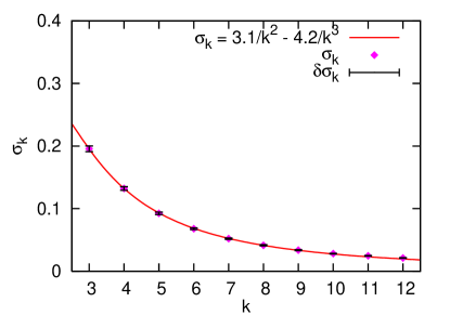
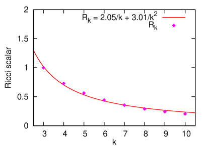
Figure 1: $\sigma_{k}$ and Ricci scalars.

In Fig. 1 we plot the values $\sigma_{k}$ defined in (27) for $k=3,\ldots,12$. The error bars for each value are the corresponding standard deviations (28). We also see how the errors decrease, along with $\sigma_{k}$, for higher and higher $k$. The fit in Fig. 1 is a curve of type

$$\sigma_{k}=\frac{\alpha}{k^{2}}+\frac{\beta}{k^{3}}+\mathrm{O}\left(\frac{1}{k^{4}}\right),$$

as we expect from the theory.

We can also study the local behavior of $\eta_{k}$ by restricting it to a subspace. Given our quintic 3-fold, we consider the rational curve defined by

$$(Z_{0}=z_{0},\,Z_{1}=-z_{0},\,Z_{2}=z_{1},\,Z_{3}=0,\,Z_{4}=-z_{1}),$$ (29)

where $Z_{i}$ are homogeneous coordinates on $\mathbb{P}^{4}$, while $(z_{0},\,z_{1})$ are homogeneous coordinates for $\mathbb{P}^{1}$. This rational curve lies on every quintic defined by Eq. (21).

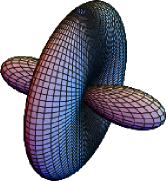
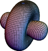
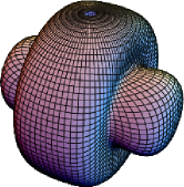
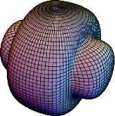
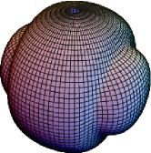
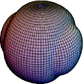
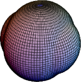
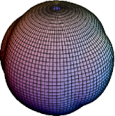
Figure 2: The values of $\eta$ on the rational curve, for $k=1$, 3, 4, 5, 7, 9, 11 and 12.

In Fig. 2 we plot the values of function $\eta_{k}$ restricted to the rational curve defined above for 12 different values of $k$, ranging between $1$ and $12$. More concretely, given the embedding (29), we choose the local coordinate system on $\mathbb{P}^{1}$ defined by $t=z_{1}/z_{0}$, and take the stereographic projection of the $t$-plane. Using spherical coordinates $(\theta,\,\phi)$ on ${\mathbb{P}}^{1}\equiv S^{2}$ we embed it into $\mathbb{R}^{3}$, by the parameterization

$$z_{0}=\sin\theta\,\cos\phi,\qquad z_{1}=\sin\theta\,\sin\phi+i\,\cos\theta.$$

In the radial direction of $\mathbb{R}^{3}$ we plot the function $\eta_{k}$. As expected, $\eta_{k}$ approaches the constant function 1 as $k$ increases.

4.2 Ricci scalars

Next we discuss how we compute the Ricci scalar on $X$. The Kähler potential on $X$ is given by the restriction of the Kähler potential (5), which is associated to a balanced metric. The metric and Ricci curvature on $X$ are given by

$$g_{h}=\partial\bar{\partial}K_{h},\qquad Ric=\partial\bar{\partial}\det{g_{h}}.$$ (30)

To compute these quantities we need the first and second derivatives of the sections $s_{\alpha}$ with respect to the coordinates of $X$. We can compute these derivatives algebraically, using the ideas outlined in Section 3.4.2. To get the actual value of $g$ and $Ric$, at a specific point $x\in X$, we evaluate our numerical expressions at this point. Let us stress that this way $g$ and $Ric$ are evaluated algebraically, without numerical derivatives.

Let us now discuss the effect of the parameter $k$ on the Ricci scalar $R$. The theoretical estimate predicts a vanishing of $R$ for large $k$ as

$$||R_{k}||<\frac{\gamma}{k}+\frac{\delta}{k^{2}}+\cdots,$$ (31)

where $\gamma$ and $\delta$ are constants, in any $C^{r}$ norm. We can see this pointwise, after a short statistical analysis. Let us pick $100$ randomly chosen points $P_{i}$ on the 3-fold, and compute the associated sets of Ricci scalars $R_{k}$, for $k\in[3,\dots,10]$. To obtain a normalized set $\tilde{R}_{k}$ of Ricci scalars we rescale all $R_{k}$ by $1/R_{3}$, and we do this for every point. This normalization leads to a more meaningful comparison between the different points.

We are only interested in points where $\tilde{R}_{k}$ shows a generic behaviour. For this we compute the expectation value of $|\tilde{R}_{10}|$ ($k=10$ gives a good accuracy)

$$\langle|\tilde{R}_{10}|\rangle=\frac{1}{100}\sum_{i=1}^{100}|\tilde{R}_{{10}}(P_{i})|=0.48.$$

We consider a point $P$ generic if it lies at a distance of order one from the mean $\langle|\tilde{R}_{10}|\rangle$, that is

$$|\tilde{R}_{{10}}(P)-\langle|\tilde{R}_{10}|\rangle|<0.5.$$

We find that $95$ points out of $100$ obey this condition. We use these $95$ points for our statistical check of Eq. (31). In Fig. 1 we plot $\langle|\tilde{R}_{k}|\rangle$ as a function of $k$. We do a least square fit for both $\gamma$ and $\delta$, and obtain very good agreement.

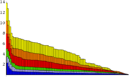
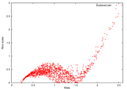
Figure 3: Histogram of Ricci scalars, and scattered plot of mass versus the Ricci scalars.

We can obtain a visual picture of how the Ricci scalars decrease with $k$ by plotting them on a histogram. We use the same $100$ points from above. To keep the picture simple we plot only six $k$ values: 3, 4, 5, 7, 9 and 12. Unlike earlier, here we do not normalize the Ricci scalars pointwise, instead we reorder them decreasingly. This ordering is done for no other reason but to enhance the visual clarity. Accordingly, in the first graph of Fig. 3 we plotted the value of the Ricci scalar for every point (the $y$ axis is the absolute value of Ricci scalar, while on the $x$ axis we have the points from 1 to 100). We did this for the $k$ values indicated above, and used different colors to distinguish them (e.g., yellow corresponds to $k=3$, while $k=12$ is blue). It is evident from this graph that by going from $k=3$ to $k=12$ the Ricci scalars decrease by an order of magnitude, in line with the theoretical expectation.

One observes that for any $k$ there are a few anomalously large Ricci scalars. To understand this we can do a scattered plot of the mass of that point versus the Ricci scalar in question (we present this for $k=12$), using $1000$ random points. This is the second graph in Fig. 3. The picture shows a correlation between large values of the Ricci scalar and large values of the mass (large in a logarithmic sense). In other words, in regions where our point generator needs large correction, via the mass, the balanced metric is a less accurate approximation of the Ricci flat metric, compared to points with smaller mass. This fact is then amplified by the formula for the Ricci tensor in Eq. (30), where the logarithmic scale is also supplied.

Finally let us note that $1/\eta_{1}$ is precisely the mass function (10). This is because the $k=1$ balanced matrix is proportional to the identity, a consequence of the discrete symmetries present for our quintic. This leads to an alternative interpretation for the first graph ($k=1$) in Fig. 2, as depicting the inverse masses of the points on that rational curve.

4.3 Discussion

We will discuss further applications of these results elsewhere; here we discuss the advantages and limitations of this approach compared to others, for example position space methods [20].

The runtime of a computation of the balanced metric can be approximated as

$$T=N_{it}\times N_{p}\times S^{2},$$

where $S$ is the number of independent sections (taking into account discrete symmetry), $N_{p}$ is the number of points used in the Monte Carlo integration, and $N_{it}$ is the number of iterations of the T-map required for convergence. Since convergence is exponential, this leads to a rough scaling with the accuracy as

$$T\sim\frac{\log\epsilon}{\epsilon^{2}}S^{2}.$$

The value of $S$ required for a given accuracy depends on the symmetries and dimension. For the balanced metrics, we expect to need $k\sim 1/\sqrt{\epsilon}$; as discussed in section 2 this could probably be improved by choosing a different scheme if accuracy were paramount. For hypersurfaces in $n$ complex dimensions, we then have $S\sim N\sim k^{n+1}$, leading to a rough overall scaling of $T\sim 1/\epsilon^{n+3}$. This might be compared with a (naive) $T\sim 1/\epsilon^{2n}$ for position space methods, so the two appear generally competitive. However, along with the other advantages we mentioned, we believe the approach we are discussing is far easier to program, and requires relatively little effort to adapt to different manifolds, and related problems such as hermitian Yang-Mills.

Since the sections $s_{\alpha}$ of $\mathcal{O}_{X}(k)$ are degree $k$ polynomials, this basis is a simple type of Fourier or momentum space basis. Very roughly speaking, a degree $k$ basis should be able to represent arbitrary structures on length scales down to $1/k$. They are particularly well suited for approximating smooth functions, as the Fourier coefficients of such a function fall off faster than any power of $k$ (see the appendix of [8] for more precise statements). This is advantageous as the Ricci flat metric is smooth, suggesting that other approximation schemes could do better than $\epsilon\sim 1/k^{2}$.

On the other hand, in some limits (say a conifold limit) the metric can develop structure on small scales, which might not be well represented by a fixed $k$ basis. This is also a problem for position space methods with a fixed lattice; there one deals with it by multi-scale methods, for example allowing the lattice spacing and structure to vary over the manifold. This is very powerful but also very intricate to program. In the present context, rather than increase $k$, one might look for analogous simplifications; either a multi-scale method which uses different $k$ in different regions (or even some sort of wavelet-inspired method). Or, since we have many explicit expressions for Ricci flat metrics near singularities, it might be useful to develop a way to patch these solutions into the global approximate solutions we discussed.

On the computer code

Our numerics is based on code that has been written entirely in C++. Our experience shows that these computations must be done in a compiled language, rather than an interpreted one. We have made extensive use of the following Boost libraries: uBlas, random, bind and thread. These libraries are on par with Fortran code, due to implementation techniques using expression templates and template metaprograms. The computations were done on an Athlon 64 4800+ dual core machine, with 4GB memory. The computational time ranges from minutes, for low $k$, to hours, and eventually 2 days (for $k=12$).

Acknowledgments

This research was supported in part by the DOE grant DE-FG02-96ER40949.

References

- [1] S. T. Yau, “On the Ricci curvature of a compact Kähler manifold and the complex Monge-Ampère equation. I,” Comm. Pure Appl. Math. 31 (1978), no. 3, 339–411.
- [2] G. Tian, “On a set of polarized Kähler metrics on algebraic manifolds,” J. Differential Geom. 32 (1990), no. 1, 99–130.
- [3] J.-P. Bourguignon, P. Li, and S.-T. Yau, “Upper bound for the first eigenvalue of algebraic submanifolds,” Comment. Math. Helv. 69 (1994), no. 2, 199–207.
- [4] H. Luo, “Geometric criterion for Gieseker-Mumford stability of polarized manifolds,” J. Differential Geom. 49 (1998), no. 3, 577–599.
- [5] S. Zelditch, “Szego kernels and a theorem of Tian,” Internat. Math. Res. Notices (1998), no. 6, 317–331.
- [6] S. K. Donaldson, “Scalar curvature and projective embeddings. I,” J. Differential Geom. 59 (2001), no. 3, 479–522.
- [7] S. K. Donaldson, “Scalar curvature and projective embeddings. II,” Q. J. Math. 56 (2005), no. 3, 345–356, math.DG/0407534.
- [8] S. K. Donaldson, “Some numerical results in complex differential geometry,” math.DG/0512625.
- [9] M. R. Douglas, R. L. Karp, S. Lukic, and R. Reinbacher, “Numerical solution to the hermitian Yang-Mills equation on the Fermat quintic,” hep-th/0606261.
- [10] M. R. Douglas, R. L. Karp, S. Lukic, and R. Reinbacher, “The Kahler potential in heterotic string compactifications,”. To appear.
- [11] R. P. Thomas, “Notes on GIT and symplectic reduction for bundles and varieties,” math.AG/0512411.
- [12] T. Mabuchi, “Extremal metrics and stabilities on polarized manifolds,” math.DG/0603493.
- [13] Y. Sano, “Numerical algorithm for finding balanced metrics,”. Tokyo Institute of Technology Preprint, 2004.
- [14] W. H. Press, S. A. Teukolsky, W. T. Vetterling, and B. P. Flannery, Numerical recipes in C++. Cambridge University Press, Cambridge, 2002. The art of scientific computing, 2nd edition.
- [15] B. Shiffman and S. Zelditch, “Distribution of zeros of random and quantum chaotic sections of positive line bundles,” Comm. Math. Phys. 200 (1999), no. 3, 661–683, math.CV/9803052.
- [16] B. Shiffman and S. Zelditch, “Number variance of random zeros on complex manifolds,” math.CV/0608743.
- [17] P. Griffiths and J. Harris, Principles of algebraic geometry. Wiley-Interscience [John Wiley & Sons], New York, 1978. Pure and Applied Mathematics.
- [18] E. Durand, Solutions numériques des équations algébriques. Tome I: Équations du type ; racines d’un polynôme. Masson et Cle, Editeurs, Paris, 1960.
- [19] I. O. Kerner, “Ein Gesamtschrittverfahren zur Berechnung der Nullstellen von Polynomen,” Numer. Math. 8 (1966) 290–294.
- [20] M. Headrick and T. Wiseman, “Numerical Ricci-flat metrics on K3,” Class. Quant. Grav. 22 (2005) 4931–4960, hep-th/0506129.