ON SHOCK WAVES IN MODELS
WITH V-SHAPED POTENTIALS

Abstract

The recently found shock wave solution in the scalar field model with the field potential $V(\phi)=|\phi|$ is generalized to the case $V(\phi)=|\phi|-\frac{1}{2}\lambda\phi^{2}$. We find two kinds of the shock waves, which are analogous of compression and expansion waves. The dependence of the waves on the parameter $\lambda$ is investigated in detail.

03.50 Kk, 05.45.-a, 11.10.Lm

1 Introduction

Interesting and still poorly studied group of field-theoretic models are these with V-shaped potentials. Physical systems with just few degrees of freedom and V-shaped potential are studied quite frequently. There are numerous results for systems such as e.g. bouncing oscillators. These systems are mainly studied in context of chaotical behaviour and grazing bifurcation [1-7]. The V-shaped potentials appear in research of plasma physics [8]. Furthermore, they can play an important role in pinning phenomena which can describe a process of vortices attaching to lines of impurities [9,10]. Apart from the applications, they are also very interesting on purely theoretical grounds because of scale invariance of vacuum sector, [11].

There are only few analytical results for the field-theoretic models with V-shaped potentials. An example of such model, which originally derives from a mechanical system, has been proposed in [12]. The model considered there is obtained as a continuum limit of the system of coupled pendulums that are allowed to take the angular positions belonging to the interval [$-\phi_{0}$, $\phi_{0}$]. This leads to appearance of a V-shaped potential, and consequently to nontrivial dynamics of the system. The angle $\phi=0$ corresponds to the pendulum in upward vertical position. A simpler model has been proposed in [11]. It derives from coupled system of bouncing balls. The potential in that model has the form $V(\phi)=|\phi|$. It can be regarded as a limit case of a large group of V-shaped symmetric potentials.

In the present paper we consider the classical scalar field model with the potential $V(\phi)=|\phi|-\frac{1}{2}\lambda\phi^{2}$, where $\lambda$ is a real constant. Such potentials with $\lambda\neq 0$ naturally appear in the case of system of coupled pendulums [12], as well as in the system of bouncing coupled balls obtained from system studied in [11] by adding new couplings, see Fig.2. Specifically, we investigate shock wave solutions. In the particular case of $\lambda=0$ they have been discussed in [13].

The field-theoretic model with the potential $|\phi|$ has special symmetry. If $\phi(x,t)$ is solution of equation of motion, then $\nu^{2}\phi(\frac{x}{\nu},\frac{t}{\nu})$, where $\nu$ is a positive constant, obeys this equation as well, see [13]. This symmetry is "on shell" type because the action functional is not invariant with respect to the scaling transformation. In general, in real physical system, apart from term $|\phi|$, the V-shaped potential has also another terms. A squared term is an example of the simplest perturbation that breaks the scaling symmetry. Investigation of effects of such perturbation is a very important issue.

Our paper is organized as follows. In Sec.2 we show connections between the model and physical systems. Next section contains analysis of solutions that have the properties of expansion shock waves. In Sec.4 we investigate symmetric compression shock waves. Sec.5 summarizes the paper.

2 The modified model and related physical systems

2.1 General definition

Let us consider the model of a real scalar field $\phi$ in one dimension. The Lagrangian has the form

$$L=\frac{1}{2}(\partial_{t}\phi)^{2}-\frac{1}{2}(\partial_{x}\phi)^{2}-V(\phi),$$ (1)

where $\phi=\phi(x,t)$ depends on rescaled position $x$ and time $t$ which are dimensionless. The potential has the form

$$V(\phi)=|\phi|-\frac{1}{2}\lambda\phi^{2}.$$ (2)

The evolution equation which corresponds to Lagrangian (1) has the form

$$(\partial^{2}_{t}-\partial^{2}_{x})\phi+\hbox{sign}(\phi)-\lambda\phi=0.$$ (3)

Because of sign function equation (3) is clearly nonlinear one. We assume that $\hbox{sign}(0)=0$. There are three qualitatively different cases: $\lambda>0$, $\lambda<0$, and $\lambda=0$ when we have the canonical model considered in [11,13].

2.2 Positive values of $\lambda$

Let us start from the case $\lambda>0$. It is convenient to set $\lambda=\rho^{2}$. The equation of motion for this case takes the form

$$(\partial^{2}_{t}-\partial^{2}_{x})\phi+\hbox{sign}(\phi)-\rho^{2}\phi=0.$$ (4)

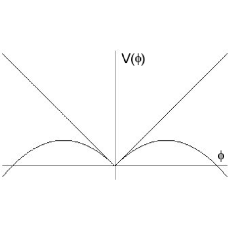
Figure 1: The potential $V(\phi)$ ($\lambda>0$) and its limit for $\lambda=0$.

The potential has one local minimum at $\phi=0$ and two local maxima at $\phi=\pm\frac{1}{\rho^{2}}$, see Fig.1. It is not differentiable at its minimum (right-hand side and left-hand side derivatives are not equal at this point). Equation (4) can be obtained from equation of motion which describes a small perturbation around the ground state in the model considered in [12]. Physical values of perturbation are given by $|\phi|$.

2.3 Negative values of $\lambda$

It turns out that the model for $\lambda<0$ has also a physical meaning. Physical system which is related to this model can be obtained from the system considered in [11] by adding new springs that link every ball with the floor, see Fig.2.

Figure 2: The system of bouncing balls.

In this system every ball can move only in vertical direction. There is a rigid floor at $\phi=0$ and every ball bounces elastically from the floor. After taking few standard steps (continuous limit, folding transformation) we get the system which dynamics is described by the equation

$$(\partial^{2}_{t}-\partial^{2}_{x})\phi+\hbox{sign}(\phi)+\sigma^{2}\phi=0,$$ (5)

where $-\infty<\phi<\infty$ whereas physical position of the balls are given by $|\phi|$. As above, we have set $\lambda=-\sigma^{2}$. The potential Fig.3 has one minimum and no local maxima.

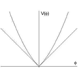
Figure 3: The potential $V(\phi)$ ($\lambda<0$) and its limit for $\lambda=0$.

2.4 On regularized potentials

In our model at $\phi=0$ first derivative of the potential does not exist at all. It is possible to replace the sharp potential by a regularized potential where instead of $|\phi|$ we use e.g. $\sqrt{\phi^{2}+\varepsilon^{2}}$ or $\varepsilon\ln{\cosh{\frac{\phi}{\varepsilon}}}$, what gives well defined first derivative at $\phi=0$. We are not interested in regularized potential in this paper because physical systems that we consider here give rather sharp than regularized potential. Another reason is that for the regularized potential only solutions such that $|\phi|\gg\varepsilon$ can survive the limit $\varepsilon\rightarrow 0$. Finding any such solution of the equation (3) with the regularized potential seems to be a very difficult task.

3 Symmetric shock waves inside the light cone

3.1 The Ansatz

Equation (3) includes term with derivatives in the form of d’Alembert operator so it can be reduced to an ordinary differential equation by assumption $\phi(x,t)=W(z)$, where $z=(x^{2}-t^{2})/4$.

There are two qualitatively different cases ($z<0$ and $z>0$) for the canonical model ($\lambda=0$). When $z<0$ the pieces of solution can be combined together in one solution. In opposite case whole solution can be either positive or negative and it is not limited respectively from above or from below. It is physically reasonable to get rid of unstable solutions. It can be simply done by modification our Ansatz to the following one $\phi(x,t)=\Theta(-z)W(z)$, where $\Theta(-z)$ is well known Heaviside step function. This modification introduces discontinuities at $x=\pm t$.

In the modified model, especially for $\lambda>0$ there are solutions for $z>0$ that are limited both from above and from below so this time we can not simply get rid of them. In further part of our work we analyze solutions for $z<0$ and $z>0$ separately because the solution inside the light cone is completely independent of the solution outside it. It is executed by assumptions $\phi(x,t)=\Theta(-z)W(z)$ and $\phi(x,t)=\Theta(z)W(z)$.

Apart from possibility of reduction equation (3) to an ordinary differential equation, an important question is whether discontinuities in our model can move with velocity $v\neq 1$ or not. To answer it let us consider $\phi(x,t)=\Theta(-z)W(z)$, where $z=pq$, $p=(x-vt)/2$, $q=(x+vt)/2$ and $v\neq 0$. Equation (3) takes the form

$$\Theta(-z)\left[A(p,q)W^{\prime\prime}-\frac{1}{2}(v^{2}+1)(zW^{\prime\prime}+W^{\prime})+\hbox{sign}(W)-\lambda W\right]+$$

$$-2\delta(z)A(p,q)W^{\prime}(z)-\delta^{\prime}(z)A(p,q)W(z)=0,$$

where

$$A(p,q)=\frac{1}{4}(v^{2}-1)(p^{2}+q^{2}),$$

and ${}^{\prime}=\frac{d}{dz}$. The terms proportional to $\Theta(-z)$, $\delta(z)$ and $\delta^{\prime}(z)$ have to vanish independently. At $z=0$ and $v\neq 1$, $W(0)=0$ and $W^{\prime}(0)=0$ because $A(p,q)\neq 0$. It means that $\phi(x,t)$ can not be discontinuous function unless $v=1$. We can see that velocity $v=1$ is distinguished by the model and it is the only admissible velocity with which discontinuities can move.

3.2 Equations of motion

Let us consider the Ansatz

$$\phi(x,t)=\Theta(-z)W(z),\qquad\hbox{where}\qquad z=\frac{1}{4}(x^{2}-t^{2}).$$ (6)

Applying Ansatz (6) to equation (3) we get the following differential equation

$$zW^{\prime\prime}+W^{\prime}-\hbox{sign}(W)+\lambda W=0.$$ (7)

Let us introduce a new variable $y$ which is related to $z$ in the following way

$$z=-\frac{1}{4}y^{2}.$$ (8)

Consequently, equation (7) acquires more familiar form

$$G^{\prime\prime}+\frac{1}{y}G^{\prime}-\rho^{2}G=-\hbox{sign}(G),\qquad\lambda>0$$ (9)

or

$$F^{\prime\prime}+\frac{1}{y}F^{\prime}+\sigma^{2}F=-\hbox{sign}(F),\qquad\lambda<0.$$ (10)

Equations (9) and (10) are Bessel equations with the signum nonlinearity. We have denoted $W(-\frac{1}{4}y^{2})=G(y)$ for positive values of $\lambda$ and $W(-\frac{1}{4}y^{2})=F(y)$ for opposite case.

3.3 Solutions for $\lambda>0$

The term $\hbox{sign}(G)$ is constant (equal $\pm 1$) on the intervals where sign of $G(y)$ is constant. Equation (9) has the solutions:

$$G_{+}(y) = \frac{1}{\rho^{2}}-\alpha I_{0}(\rho y)-\beta K_{0}(\rho y)\,\,\,\,\,\qquad\hbox{for}\qquad G(y)>0,$$

$$G_{-}(y) = -\frac{1}{\rho^{2}}+\widetilde{\alpha}I_{0}(\rho y)+\widetilde{\beta}K_{0}(\rho y)\qquad\hbox{for}\qquad G(y)<0,$$

where $\alpha,\beta,\widetilde{\alpha},\widetilde{\beta}$ are arbitrary constants. We will find these coefficients matching pieces of solution so as to obtain a solution that is valid on full available range of $y$. Physically, only real solutions are interesting so only $y\geq 0$ is considered. It is convenient to introduce the coefficients $\alpha_{k}$ and $\beta_{k}$ and combine all the solutions in one formula

$$G_{k}(y)=(-1)^{k}\left(\frac{1}{\rho^{2}}-\alpha_{k}I_{0}(\rho y)-\beta_{k}K_{0}(\rho y)\right),$$ (11)

where $k=0,1,2,\ldots$. We assume that $G_{0}(y)$, that is $G_{+}$ type, starts from $y=0$. It does not cause loosing of generality because physically relevant quantity is $|\phi|$, thus case where $G_{-}(y)$ plays role of solution that start from $y=0$ does not have to be extra discussed. For $G_{0}(y)$ the coefficient $\beta_{0}$ has to vanish to ensure regularity at $y=0$. The coefficient $\alpha_{0}$ can be expressed with help of $G_{0}(0)$, and then $G_{0}(y)$ takes the form

$$G_{0}(y)=\frac{1}{\rho^{2}}-\left(\frac{1}{\rho^{2}}-G_{0}(0)\right)I_{0}(\rho y).$$ (12)

For fixed $\rho$ there are three qualitatively different cases depending on $G_{0}(0)$.

Figure 4: The unstable symmetric shock wave at t=2.

Figure 5: The unstable symmetric shock wave at t=5.

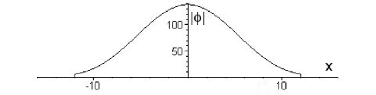
Figure 6: The unstable symmetric shock wave at t=12.

For $G_{0}(0)>\frac{1}{\rho^{2}}$ the solution $G_{0}(y)\rightarrow\infty$ for $y\rightarrow\infty$ (unstable solution). In this case solution $G_{0}(y)$ cover whole range $y\geq 0$. The shape of the shock wave for $\rho=0.5$ and $G_{0}(0)=6.0$ at different times is shown in Figs.4-6.

In the case $G_{0}(0)=\frac{1}{\rho^{2}}$ we obtain the shock wave

$$\phi(x,t)=\frac{1}{\rho^{2}}\Theta(t^{2}-x^{2}).$$

For this wave, values of the field behind the wave front are constant and equal $1/\rho^{2}$.

Last case $G_{0}(0)<\frac{1}{\rho^{2}}$ is more complicated but it is much more interesting. The solution $G_{0}(y)$ holds only on the interval $0\leq y<b_{0}$, where $G_{0}(y)>0$. For fixed $G_{0}(0)$, the first zero of $G(y)$ i.e. $b_{0}$ is determined by solution of following equation

$$I_{0}(\rho b_{0})=\frac{1}{1-G_{0}(0)\rho^{2}}.$$

Unfortunately, it can be solved only numerically. It is clear that $b_{0}$ depends on $\rho$. For given $b_{0}$ first piece of solution $G(y)$ takes the form

$$G_{0}(y)=\frac{1}{\rho^{2}}\left[1-\frac{I_{0}(\rho y)}{I_{0}(\rho b_{0})}\right].$$ (13)

We are interested in a solution for all nonnegative values of $y$. Having pieces of solution (11) and matching conditions

$$G_{k}(b_{k-1})=0,\qquad G^{\prime}_{k}(b_{k-1})=G^{\prime}_{k-1}(b_{k-1}),$$ (14)

which are implied by equation (9) we can calculate coefficients $\alpha_{k}$ and $\beta_{k}$. First matching condition allows to eliminate coefficients $\beta_{k}$. Solution (11) takes the form

$$G_{k}(y) = (-1)^{k}\left[\frac{1}{\rho^{2}}\left(1-\frac{K_{0}(\rho y)}{K_{0}(\rho b_{k-1})}\right)\right.$$ (15)

$$- \alpha_{k}I_{0}(\rho b_{k-1})\left.\left(\frac{I_{0}(\rho y)}{I_{0}(\rho b_{k-1})}-\frac{K_{0}(\rho y)}{K_{0}(\rho b_{k-1})}\right)\right].$$

The zeros $b_{k}$ for $k=1,2,\ldots$ come from the equation $G_{k}(b_{k})=0$. Like for $k=0$ we can get them numerically. The second condition in (14) gives coefficients $\alpha_{k}$:

$$\alpha_{1}=\frac{1}{\rho^{2}I_{0}(\rho b_{0})}\frac{\mathcal{K}(b_{0},b_{0})-\rho^{2}\alpha_{0}I_{1}(\rho b_{0})}{\mathcal{I}(b_{0},b_{0})+\mathcal{K}(b_{0},b_{0})}$$

$$\alpha_{k}=\frac{1}{\rho^{2}I_{0}(\rho b_{k-1})}\left[A-\rho^{2}I_{0}(\rho b_{k-2})B\right],$$

where

$$A\equiv\frac{\mathcal{K}(b_{k-1},b_{k-2})+\mathcal{K}(b_{k-1},b_{k-1})}{\mathcal{I}(b_{k-1},b_{k-1})+\mathcal{K}(b_{k-1},b_{k-1})},$$

$$B\equiv\frac{\mathcal{I}(b_{k-1},b_{k-2})+\mathcal{K}(b_{k-1},b_{k-2})}{\mathcal{I}(b_{k-1},b_{k-1})+\mathcal{K}(b_{k-1},b_{k-1})}.$$

and $k=2,3,\ldots$. We have introduced the special notation

$$\mathcal{I}(x,y)\equiv\frac{I_{1}(\rho x)}{I_{0}(\rho y)},\qquad\mathcal{K}(x,y)\equiv\frac{K_{1}(\rho x)}{K_{0}(\rho y)}.$$

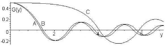
Figure 7: The solutions $G(y)$ for fixed $G_{0}(0)=0.5$ and different values of $\rho$. The curve $A$ correspond to $\rho=0.1$, $B$ to $\rho=0.5$ and curve $C$ is the solution for $\rho=1.4$. For fixed $G_{0}(0)$ the parameter $\rho$ belongs to the interval $0<\rho<1/\sqrt{G_{0}(0)}$.

The zeros of $G(y)$ depend on $\rho$ - they are larger for larger values of $\rho$, Fig.7. For fixed $G_{0}(0)$ and $\rho\rightarrow G_{0}(0)^{-1/2}$ first zero $b_{0}\rightarrow\infty$ and, of course, $b_{k}\rightarrow\infty$ ($b_{0}<b_{1}<b_{2}<\ldots$). All the zeros $b_{k}$ are larger than their counterparts $a_{k}$ in the canonical model. It means that zeros $x_{k}=\pm\left(t^{2}-b_{k}^{2}\right)^{1/2}$ in the modified model run faster than $x^{c}_{k}=\pm\left(t^{2}-a_{k}^{2}\right)^{1/2}$ in the canonical model. A pair of zeros $x_{k}$ appears at $t=b_{k}$ and moves with velocities $v_{k}=\pm\left(1-b_{k}^{2}/t^{2}\right)^{-1/2}$. In Fig.8-10 we present three snapshots which show the symmetric shock wave for $G_{0}(0)<\frac{1}{\rho^{2}}$.

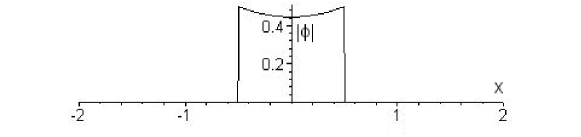
Figure 8: The symmetric shock wave for $\rho=0.5$, $G_{0}(0)=0.5$ at t=0.5.

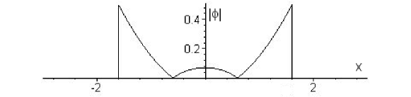
Figure 9: The symmetric shock wave for $\rho=0.5$, $G_{0}(0)=0.5$ at t=1.6.

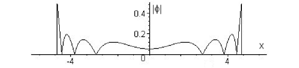
Figure 10: The symmetric shock wave for $\rho=0.5$, $G_{0}(0)=0.5$ at t=4.7.

3.4 Solutions for $\lambda<0$

This section is devoted to presentation of solutions correspond to equation (10). Many steps are the same so we sometimes skip the comments. Let us start from the solution of (10) given in the form

$$F_{k}(y)=(-1)^{k}\left(\mu_{k}J_{0}(\sigma y)+\nu_{k}Y_{0}(\sigma y)-\frac{1}{\sigma^{2}}\right),$$ (16)

where $J_{0}$ and $Y_{0}$ are Bessel functions. They take real values for $y\geq 0$. $F_{k}(y)$ are positive for $k=0,2,4,\ldots$ and negative for $k=1,3,5,\ldots$. We assume that $F_{0}(y)$ starts from $y=0$. This time, for given $\sigma$ there is no qualitatively change in behaviour of solution for different $F_{0}(0)$. $F_{0}(y)$ can be expressed in the form

$$F_{0}(y)=\left(F_{0}(0)+\frac{1}{\sigma^{2}}\right)J_{0}(\sigma y)-\frac{1}{\sigma^{2}}.$$ (17)

The first zero $c_{0}$ is calculated from the equation $F_{0}(c_{0})=0$. We can rewrite $F_{0}(y)$ using $c_{0}$

$$F_{0}(y)=\frac{1}{\sigma^{2}}\left[\frac{J_{0}(\sigma y)}{J_{0}(\sigma c_{0})}-1\right].$$ (18)

In order to have solution for whole range $y\geq 0$ we have to calculate $\mu_{k}$ and $\nu_{k}$. We use the matching conditions

$$F_{k}(c_{k-1})=0,\qquad F^{\prime}_{k}(c_{k-1})=F^{\prime}_{k-1}(c_{k-1}).$$ (19)

For $k=1,2,\ldots$

$$F_{k}(y) = (-1)^{k+1}\left[\frac{1}{\sigma^{2}}\left(1-\frac{Y_{0}(\sigma y)}{Y_{0}(\sigma c_{k-1})}\right)-\right.$$ (20)

$$- \left.\mu_{k}J_{0}(\sigma c_{k-1})\left(\frac{J_{0}(\sigma y)}{J_{0}(\sigma c_{k-1})}-\frac{Y_{0}(\sigma y)}{Y_{0}(\sigma c_{k-1})}\right)\right].$$

The coefficients $\nu_{k}$ have been eliminated by using first condition in (19). The zeros $c_{k}$ fulfil the equation $F_{k}(c_{k})=0$. Second condition in (19) gives coefficients $\mu_{k}$

$$\mu_{1}=-\frac{1}{\sigma^{2}J_{0}(\sigma c_{0})}\frac{\mathcal{Y}(c_{0},c_{0})+\mu^{2}\mu_{0}J_{1}(\rho c_{0})}{\mathcal{J}(c_{0},c_{0})-\mathcal{Y}(c_{0},c_{0})}$$

$$\mu_{k}=-\frac{1}{\sigma^{2}J_{0}(\sigma c_{k-1})}\left[\widetilde{A}+\sigma^{2}J_{0}(\sigma c_{k-2})\widetilde{B}\right],$$

where $k=2,3,\ldots$ and

$$\widetilde{A}\equiv\frac{\mathcal{Y}(c_{k-1},c_{k-2})+\mathcal{Y}(c_{k-1},c_{k-1})}{\mathcal{J}(c_{k-1},c_{k-1})-\mathcal{Y}(c_{k-1},c_{k-1})}$$

$$\widetilde{B}\equiv\frac{\mathcal{J}(c_{k-1},c_{k-2})-\mathcal{Y}(c_{k-1},c_{k-2})}{\mathcal{J}(c_{k-1},c_{k-1})-\mathcal{Y}(c_{k-1},c_{k-1})}.$$

By analogy, the functions $\mathcal{J}$ and $\mathcal{Y}$ are defined by formulas

$$\mathcal{J}(x,y)\equiv\frac{J_{1}(\sigma x)}{J_{0}(\sigma y)},\qquad\mathcal{Y}(x,y)\equiv\frac{Y_{1}(\sigma x)}{Y_{0}(\sigma y)}.$$

Having $\mu_{k}$ we can find consecutive zero $c_{k}$ as the solution of the equation $F_{k}(c_{k})=0$. Fig.11 presents solutions $F(y)$ for $F_{0}(0)$ that is set and different values of $\sigma$.

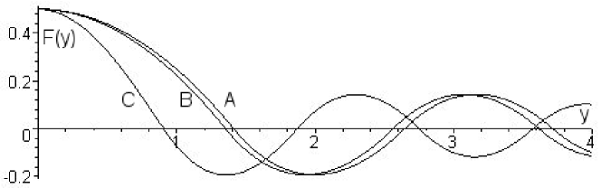
Figure 11: The solutions $F(y)$ for fixed $F_{0}(0)=0.5$ and different values of $\sigma$. The curve $A$ correspond to $\sigma=0.1$, $B$ to $\sigma=0.5$ and curve $C$ to $\sigma=2.0$.

The zeros $c_{k}$ are smaller than in the canonical model so zeros $x_{k}=\pm(1-c_{k}^{2}/t^{2})^{1/2}$ move slower than zeros $x^{c}_{k}$. They are getting smaller for $\sigma$ being increased. The shape of $|\phi|$ qualitatively resembles that presented in Fig.8-10.

3.5 Divergence of sequences $b_{k}$ and $c_{k}$

An interesting problem is if the sequence of $b_{k}$ (or $c_{k}$) is divergent or not. Unfortunately, we can not show a proof of divergence these sequences (only a numerical evidence) because explicit expressions for $b_{k}$ ($c_{k}$) are not known - we have got them only as a result of numerical computations. To see it, we introduce

$$b_{n}=b_{0}x_{1}x_{2}\cdot\ldots\cdot x_{n},\qquad\hbox{where}\qquad x_{k}=\frac{b_{k}}{b_{k-1}}.$$

Let us say that for $n\rightarrow\infty$ the sequence of $b_{n}$ is divergent $b_{n}\rightarrow\infty$. It also means that the sequence of $\ln{b_{n}}$ is divergent and sum of these logarithms

$$S_{n}=\sum_{i=1}^{n}\ln{x_{i}}$$

as well. We apply Kummer criterion so as to check if the series is divergent [16]. In our computation the comparative sequence $q_{n}=n\ln{n}$ has been used. It has been checked up to $n=700$ that

$$\mathcal{K}_{n}=q_{n}\frac{b_{n}}{b_{n+1}}-q_{n+1}$$

are negative and monotonically decrease, see Fig.12.

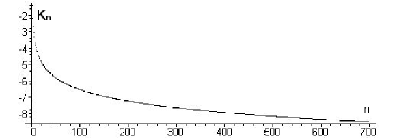
Figure 12: Behaviour of $\mathcal{K}_{n}$ for sequence $b_{n}$.

Kummer criterion says that series is divergent if for all $n>N$, values of $\mathcal{K}_{n}\leq 0$, where $N$ is a fixed number. It suggests that solution $G(y)$ covers whole $y\geq 0$. It has been checked that also the sequence of $c_{n}$ is probably divergent.

3.6 The correspondence between the modified and the canonical model

The potential $V(\phi)=|\phi|$ is the limit case of the modified one for $\lambda\rightarrow 0$. We are interested in limit $\lambda\rightarrow 0$ for the solutions in the modified model. It is not a priori clear that these limit solutions have to be solutions that are known from the canonical model. We are able to do an analytical computation for first two pieces of solution i.e. $G_{0}$ and $G_{1}$ (or $F_{0}$ and $F_{1}$). Let us remind that two first pieces of solution $W^{c}(z)$ for the canonical model have the form

$$W^{c}_{-1}(z)=z+a_{0},\qquad W^{c}_{0}(z)=-\left(z+a_{0}+2a_{0}\ln{\frac{|z|}{a_{0}}}\right),$$ (21)

where $-a_{0}$ is the first zero (for variable $z$). For more detail see [6]. Let us denote $W^{+}_{-1}(z)\equiv G_{0}(y(z))$ and $W^{+}_{0}(z)\equiv G_{1}(y(z))$ (by analogy $W^{-}_{-1}(z)\equiv F_{0}(y(z))$ and $W^{-}_{0}(z)\equiv F_{1}(y(z))$). We also rename $\rho_{+}\equiv\rho$ and $\rho_{-}\equiv\sigma$. We are interested in comparison of the canonical and the modified solution for $\rho_{\pm}\rightarrow 0$. In this limit the condition $W^{c}_{-1}(0)=W^{\pm}_{-1}(0)$ can be replaced by $a_{0}=a^{\pm}_{0}$, where $a^{+}_{0}=b^{2}_{0}/4$ and $a^{-}_{0}=c^{2}_{0}/4$. The solution $W_{-1}^{\pm}$ and $W_{0}^{\pm}$ can be expanded in the Taylor series what gives

$$W^{\pm}_{-1}(z)=z+a_{0}\mp C\rho_{\pm}^{2}+\mathcal{O}(\rho_{\pm}^{4}),$$ (22)

$$W^{\pm}_{0}(z)=-\left(z+a_{0}+2a_{0}\ln{\frac{|z|}{a_{0}}}\right)\mp D\rho_{\pm}^{2}+\mathcal{O}(\rho_{\pm}^{4}),$$ (23)

where

$$C\equiv\frac{z^{2}}{4}+a_{0}z+\frac{3}{4}a_{0}^{2},$$

$$D\equiv(a_{0}^{2}-2a_{0}z)\ln{\frac{|z|}{a_{0}}}-\frac{z^{2}}{4}+3a_{0}z+\frac{13}{4}a_{0}^{2}.$$

The leading terms in (22) and (23) do not depend on $\rho_{\pm}$ so they are limits of these solutions for $\rho_{\pm}\rightarrow 0$. The most important thing is that these limits are exactly equal to the first two solutions $W_{-1}^{c}$ and $W_{0}^{c}$ in the canonical model. The correspondence between the other solutions $W^{\pm}_{k}$ can be checked numerically. We can see that the smaller values of $k$ we take, the better correspondence is.

4 Symmetric shock waves outside the light cone

4.1 Equations of motion

The solutions outside the light cone can be obtained with help of the Ansatz

$$\phi(x,t)=\Theta(z)W(z),\qquad\hbox{where}\qquad z=\frac{1}{4}(x^{2}-t^{2}).$$ (24)

If we now introduce $z=\frac{1}{4}y^{2}$ we get

$$g^{\prime\prime}+\frac{1}{y}g^{\prime}+\rho^{2}g=\hbox{sign}(g),$$ (25)

$$f^{\prime\prime}+\frac{1}{y}f^{\prime}-\sigma^{2}f=\hbox{sign}(f),$$ (26)

where $g(y)=W(z(y))$ for $\lambda>0$ and $f(y)=W(z(y))$ for $\lambda<0$.

4.2 Case $\lambda>0$

It is convenient, for our further analysis of solutions, to associate the potential $U(g)$ with equation (25). We can easily see that $U(g)=\frac{1}{2}\rho^{2}g^{2}-|g|$, see Fig.13.

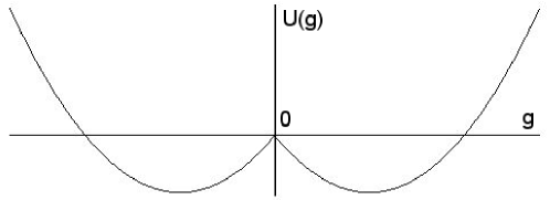
Figure 13: The potential $U(g)$.

The solution of (25) takes the form

$$g_{k}(y)=(-1)^{k}\left(\frac{1}{\rho^{2}}-\mu_{k}J_{0}(\rho y)-\nu_{k}Y_{0}(\rho y)\right),$$ (27)

where $g_{k}>0$ for $k=0,2,4,\ldots$ and $g_{k}<0$ otherwise. As above, we have to set $\nu_{0}=0$ so as to have $g_{0}(y)$ regular at $y=0$. If $g_{0}(0)$ is given then

$$g_{0}(y)=\frac{1}{\rho^{2}}-\left(\frac{1}{\rho^{2}}-g_{0}(0)\right)J_{0}(\rho y).$$ (28)

In Fig.14 we present a few curves (28) for different values of $g_{0}(0)$. There are several qualitatively different cases.

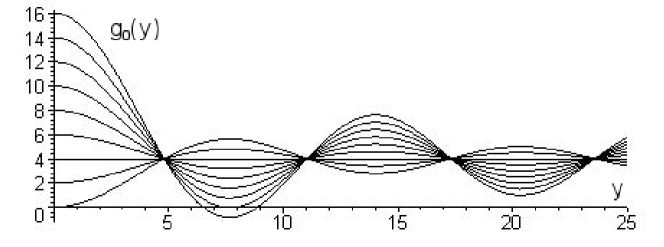
Figure 14: The curves $g_{0}(y)$ for different $g_{0}(0)$ and $\rho=0.5$. They are solution for full range $y\geq 0$ except those which start from $g_{0}(0)=14$ and $g_{0}(0)=16$.

Case $g_{0}(0)=0$ corresponds to solution that starts from the point where $U(g)$ has its local maximum. We have chosen positive solution but for $g_{0}(0)=0$, negative solution is possible as well. We can get these solutions by replacing $(-1)^{k}$ in (27) with $(-1)^{k+1}$ and assuming that $g_{0}(y)$ starts from $y=0$. We will not discuss this situation separately because $|\phi|$ is physical quantity. It is worth mentioning that this solution is not exactly shock type because there is not sharp front wave.

For $0<g_{0}(0)<g_{0}^{crit}$, where

$$g_{0}^{crit}=\frac{1}{\rho^{2}}\left(1-\frac{1}{J_{0}(j^{1}_{1})}\right)$$

the solutions $g_{0}(y)$ are valid for all $y\geq 0$. $j^{1}_{1}$ is the first zero of $J_{1}$, ($j^{0}_{1}=0$). Approximately, $\rho^{2}g^{crit}_{0}=3.482872$. This case contains the constant solution $g_{0}(y)=\frac{1}{\rho^{2}}$.

For critical value of $g_{0}(0)=g_{0}^{crit}$ the first zero of $g(y)$ appears. The solution can take either of forms: the solution

$$g_{0}(y)=\frac{1}{\rho^{2}}\left(1-\frac{J_{0}(\rho y)}{J_{0}(j^{1}_{1})}\right)$$ (29)

for all $y\geq 0$ or $g_{0}(y)$ given by (29) for $0\leq y\leq j^{1}_{1}/\rho$ and $g_{1}(y)=-g_{0}(y)$ for $y\geq j^{1}_{1}/\rho$.

If $g_{0}(y)$ is a little bit bigger than $g^{crit}_{0}$ the solution is made up of $g_{0}(y)$ and $g_{1}(y)$ but this time $j^{1}_{1}$ in (29) is replaced with $\rho c_{0}$ and $g_{1}(y)$ contains also function $Y_{0}(\rho y)$, see Fig.15. This picture is valid until $g_{0}(0)$ reach consecutive critical value $g_{0}^{crit2}$ (unfortunately, we are not able to give appropriate analytical formula - only numerical value of $g^{crit2}$ is available).

Therefore, for $g_{0}(0)=g_{0}^{crit2}$ situation resembles that for $g_{0}(0)=g_{0}^{crit}$ but this time two zeros $c_{0}$ and $c_{1}$ already exist.

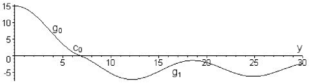
Figure 15: The solution $g(y)$ that has only one zero.

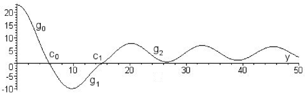
Figure 16: The solution $g(y)$ with two zeros.

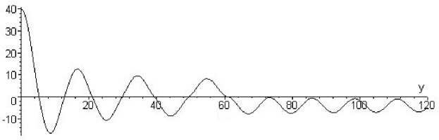
Figure 17: The solution $g(y)$ with six zeros.

For values of $g_{0}(0)$ a little bit more than $g_{0}^{crit2}$ solution looks like it was shown in Fig.16. For greater values of $g_{0}(0)$ more zeros $c_{k}$ appear, see Fig.17. An important issue is that for finite $g_{0}(0)$, maximal value of $k$ is always a finite number. For these solutions, asymptotic values of $g(y)$ for $y\rightarrow\infty$ i.e. $\pm 1/\rho^{2}$ correspond to the minima of the potential $U(g)$. We have not discussed yet the formulas for coefficients $\mu_{k}$ and $\nu_{k}$ in (27). Fortunately, they have the same form as analogical coefficients in equation (16) - only $\sigma$ has to be replaced with $\rho$.

4.3 Case $\lambda<0$

The potential $U(f)$ for equation (26) takes the form $U(f)=-\frac{1}{2}\sigma^{2}f^{2}-|f|$ what suggests unstable behaviour of $f(y)$. The solutions of (26) can be written down in the form

$$f_{+}(y) = \alpha I_{0}(\rho y)+\beta K_{0}(\rho y)-\frac{1}{\sigma^{2}}\,\,\,\,\,\qquad\hbox{for}\qquad f(y)>0,$$

$$f_{-}(y) = -\widetilde{\alpha}I_{0}(\rho y)-\widetilde{\beta}K_{0}(\rho y)+\frac{1}{\sigma^{2}}\qquad\hbox{for}\qquad f(y)<0.$$

Let us consider $f(y)>0$. By analogy to our previous analysis we will denote it as $f_{0}(y)$. For given $f_{0}(0)$ it takes the form

$$f_{0}(y)=\left(\frac{1}{\sigma^{2}}+f_{0}(0)\right)I_{0}(\sigma y)-\frac{1}{\sigma^{2}},$$ (30)

where $\beta=0$. There are five such solutions in Fig.18. The solution $f_{0}(y)$ covers whole range $y\geq 0$. We have an analogical situation for a negative solution. The border solution ($f_{0}(0)=0$) is, of course, a non-shock type.

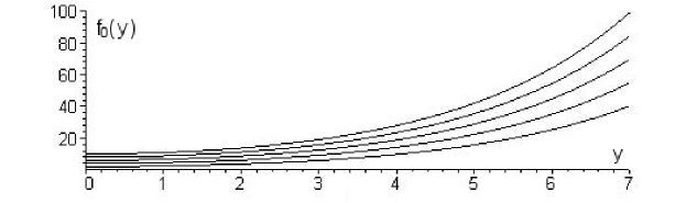
Figure 18: The solutions $f_{0}(y)$ for different (positive) values of $f_{0}(0)$.

5 Summary

We have presented the shock wave solutions in the model with the potential $V(\phi)=|\phi|-\frac{1}{2}\lambda\phi^{2}$, where $\lambda$ is a real constant. The square term plays the role of perturbation of the potential $V(\phi)=|\phi|$. The potential $|\phi|$ plays a special role because the corresponding equation of motion has the scaling symmetry. The square term is the simplest one that breaks this symmetry. It has been shown that both cases with nonzero values of $\lambda$ ($\lambda>0$ and $\lambda<0$) have physical applications - appropriate potentials appear in the system of coupled bouncing pendulums or bouncing balls.

Two kinds of waves have been found. The first one is exactly zero outside the light cone and has two wavefronts (the field is non-continuous at them) exactly at the surface of the light cone. Depending on $G_{0}(0)$ the solution inside the light cone is unstable, constant, or has isolated zeros. We have found that these zeros run faster ($\lambda>0$) or slower ($\lambda<0$) than their counterpart in the canonical model ($\lambda=0$). It has been also argued (by showing the numerical evidence) that zeros of solution, that depends on variable $y$, form probably divergent sequence. Moreover, we have shown (analytically in the case of first two pieces of solution) that shock waves inside the light cone for the modified model in the limit $\lambda\rightarrow 0$ reduce to solutions known from the canonical model.

The second type of solution has also wavefronts at $x=\pm t$. This solution takes zero values inside the light cone. There is family of solutions that asymptotically ($y\rightarrow\infty$) reach values $\pm 1/\rho^{2}$. At the points $g=\pm 1/\rho^{2}$ the potential $U(g)$ (Fig.13) has the local minima (or $V(\phi)$ has its local maxima, Fig.1). Among solutions that belong to this family, there are solutions that have no zeros, have only one zero, exactly two zeros etc. In contrast to the shock waves inside the light cone that have infinite number of zeros, solutions considered here have always finite number of zeros. There is also non-shock type solution - it has only one zero at the surface of light cone. It can be regarded as the border case of solutions belonging to this family. We have also found another family of solutions that have no zeros and grow to infinity for $y\rightarrow 0$.

6 Acknowledgements

I would like to thank Henryk Arodź for discussion and numerous valuable remarks.

References

- [1] J.M.T. Thompson and R.Ghaffari Phys. Rev., A27, 1741 (1983).
- [2] S.W. Shaw and P. Holmes Phys. Rev. Lett., 51, 323 (1983).
- [3] H. E. Nusse, E. Ott and J.A. Yorke Phys. Rev., E49, 1073 (1994).
- [4] W. Chin, E. Ott, H. E. Nusse and C. Grebogi Phys. Rev., E50, 4427 (1994).
- [5] W. Chin, E. Ott, H. E. Nusse and C. Grebogi Phys. Lett., A201, 197 (1995).
- [6] L. N. Virgin and C. J. Bagley Physica, D130, 43 (1999).
- [7] H. Dankowicz and A. B. Nordmark Physica, D136, 280 (2000).
- [8] S. Isiguro et al. Phys. Rev. Lett., 78, 4761 (1997).
- [9] D. R. Nelson "Defects and Geometry in Condense Matter Physics"
- [10] O. Narayan and D. S. Fisher Phys. Rev., B48, 7030 (1993).
- [11] H. Arodź, P. Klimas and T. Tyranowski Acta Phys. Pol, 36, 3861 (2005).
- [12] H. Arodź Acta Phys. Pol, 33, 1241 (2002).
- [13] H. Arodź, P. Klimas and T. Tyranowski Phys. Rev., E73, 046609 (2006).
- [14] H. Arodź and P. Klimas Acta Phys. Pol, 36, 787 (2005).
- [15] E. Włodarczyk "Wstęp do mechaniki wybuchu" (in Polish) [An introduction to mechanics of explosion], PWN, Warszawa, 1994, 320 pp.
- [16] G. M. Fichtenholz, Rachunek r zniczkowy i calkowy. Tom 2. (in Polish) [Differential and integral calculus. Vol. 2], Translated from the Russian by A. Goetz, L. Szamkołowicz, B. Gleichgewicht, T. Huskowski, E. Piegat. Nine Edition. PWN, Warszawa, 1985. 696 pp.