DAMTP-2006-117
ITFA-2006-48

Effective Actions for Heterotic M-Theory
Jean-Luc Lehners^†, Paul McFadden^‡ and Neil Turok^†

^† DAMTP, CMS, Wilberforce Road, CB3 0WA, Cambridge, UK.
^‡ ITFA, Valckenierstraat 65, 1018XE Amsterdam, the Netherlands.

1 Introduction

The conjectured duality of Hořava and Witten [1, 2] between eleven-dimensional supergravity compactified on the orbifold $S^{1}/\mathbb{Z}_{2}$ and strongly coupled heterotic string theory is a key development for fundamental string and M-theory, for particle phenomenology [3] and for early universe cosmology [4]. Realistic particle physics models are obtained by first compactifying six of the ten spatial dimensions on a Calabi-Yau 3-fold, taken to be smaller than the orbifold dimension for phenomenological reasons, and then studying the resulting five-dimensional effective theory [5, 6] in which one of the remaining four spatial dimensions is the orbifold with its boundary branes. In recent work, Moss has given an improved treatment of the boundary conditions for bulk fields [7, 8], giving greater confidence in this general approach.

Cosmological applications of heterotic M-theory emphasise the importance of letting the branes be fully dynamical [4, 9]. If heterotic M-theory is to describe our universe, however, then the constancy of the measured coupling constants implies that the volume of the Calabi-Yau, which is related to the gauge couplings, must have been stabilised shortly after the big bang. Similarly, the radion field measuring the size of the extra dimension must either decouple efficiently from the matter density, or itself be given a mass. Nevertheless, it is entirely reasonable to assume that the branes may have been dynamical over a short period of time just before and after the big bang. It is therefore of interest to derive four-dimensional effective actions for heterotic M-theory describing the motion of bulk and boundary branes, and many authors have done so in the past [10, 11, 12, 13, 14, 15, 16]. In particular, we would like to draw attention to [17], which is closely related to the work reported here.

We will derive the effective action in this paper by developing the moduli space approximation in light of the recently derived colliding branes solution of [18]. This exact solution of heterotic M-theory enables us to understand the global structure of moduli space in more detail. In particular, we find that there are two different types of boundaries to moduli space: the first type of boundary, which is well-known, arises for example because a bulk brane is constrained to remain in between the two orbifold branes, and therefore the range of the coordinate describing its location along the orbifold is restricted. However, when a bulk brane collides with one of the orbifold branes, a small instanton transition can occur [19], signalling the appearance of new, light degrees of freedom which cannot be described in the original four-dimensional effective theory. In other words, the original moduli space approximation cannot be trusted at these locations and an improved treatment is needed.

We will argue, however, that there may also exist boundaries to moduli space that can best be described as hard and repulsive. Such a boundary arises at a zero of the bulk warp factor. From the higher-dimensional picture, we know that it is always the negative-tension brane that encounters this singularity, and is in fact repelled by it (see Figure 1).

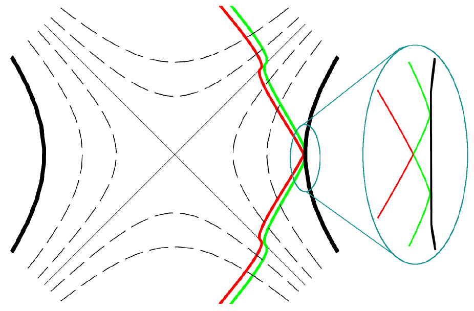
Figure 1: A Kruskal plot of the colliding branes solution described in [18]. In suitable coordinates, the bulk geometry is static and contains a timelike naked singularity (denoted by thick black lines) corresponding to a zero of the bulk warp factor. The dashed lines indicate representative orbits of the bulk Killing vector field. The boundary branes then move through this bulk geometry according to the Israel junction conditions. The trajectory of the positive-tension brane is shown in red and that of the negative-tension brane in green. The collision of the branes, as well as the two bounces of the negative-tension brane off the naked singularity, are shown at a magnified scale in the inset. The regularisation of these bounces is discussed in detail in [18].

We describe the boundary as ‘hard’ because in the presence of the slightest amount of matter on the negative-tension brane, satisfying the weak energy condition, the singularity is in fact never reached and the negative-tension brane simply bounces back smoothly. In the moduli space approximation this corresponds to a simple reflection of one of the two scalar fields off the boundary. For a small, fixed density of matter on the negative-tension brane, as we lower the speed of the incoming negative-tension brane, the bounce becomes milder and milder. In this situation, we do not expect additional light degrees of freedom, such as branes wrapping cycles of the Calabi-Yau, to become light enough to play a significant role, and we expect the four-dimensional effective description to remain accurate.

We begin this paper with a brief review of heterotic M-theory, before proceeding in Section 3 to derive the moduli space action for the case in which there is no bulk brane present. From this action, we show how to recover the colliding branes solution recently discussed in [18]. This particular solution highlights another general feature of the moduli space approximation that shows the importance of higher-dimensional input: the moduli space approach leads to an infinite number of possible background solutions. Choosing a particular one then amounts to imposing boundary conditions that are obtained from the original higher-dimensional theory. We will generalise our discussion to incorporate the presence of a bulk brane in Section 4. In particular, we exhibit a series of special cases in which the moduli space action simplifies. In these instances, we are able to recover and improve upon some earlier results appearing in the literature. We conclude in Section 5.

2 Heterotic M-Theory

Hořava-Witten theory can be dimensionally reduced on a Calabi-Yau 3-fold to yield five-dimensional heterotic M-theory [1, 2, 5, 6]. This gauged supergravity theory can be consistently truncated to gravity and a scalar $\phi$ parameterising the volume of the Calabi-Yau manifold (namely $V_{\mathrm{CY}}=e^{\phi}$). The action is given by

$$S = \int_{5d}\sqrt{-g}\,[R-\frac{1}{2}(\partial\phi)^{2}-6\alpha^{2}e^{-2\phi}]$$ (2.1)

$$+12\alpha\int_{4d,\,y=-1}\sqrt{-g}e^{-\phi}-12\alpha\int_{4d,\,y=+1}\sqrt{-g}e^{-\phi},$$

where $\alpha$ is related to the number of units of 4-form flux pointing entirely in the Calabi-Yau directions, and we have placed branes of opposite tensions at $y=\pm 1$ (where $y$ is the coordinate transverse to the branes). It is important to realise that when boundary brane actions are present $\alpha$ is necessarily non-zero. As a consequence five-dimensional Minkowski space is not the vacuum of the theory; rather, the vacuum is given by a domain wall spacetime of the form

$$\mathrm{d}s^{2} = h^{2/5}(y)\,\big{[}B^{2}\,(-\mathrm{d}\tau^{2}+\mathrm{d}\vec{x}^{2})+A^{2}\,\mathrm{d}y^{2}\big{]},$$

$$e^{\phi} = A\,h^{6/5}(y),$$

$$h(y) = 5\alpha\,y+C,$$ (2.2)

where $A$, $B$ and $C$ are arbitrary constants. The $y$ coordinate is taken to span the orbifold $S^{1}/\mathbb{Z}_{2}$ with fixed points at $y=\pm 1$. In an ‘extended’ picture of the solution, obtained by $\mathbb{Z}_{2}$-reflecting the solution across the branes, there is a downward-pointing kink at $y=-1$ and an upward-pointing kink at $y=+1$. These ensure the Israel conditions are satisfied, with the negative-tension brane being located at $y=-1$ and the positive-tension brane at $y=+1$.

3 The Moduli Space Action

In our previous paper [18], we derived the higher-dimensional solution for colliding branes in heterotic M-theory. Here, we wish to describe this solution in terms of the four-dimensional effective theory. We derive this theory by making use of the moduli space approximation, originally employed in the study of the low-energy dynamics of BPS monopoles [20, 21], and subsequently developed extensively in the mathematical literature [22]. The main idea is the following. If the set of static solutions of given topology is parameterised by some continuous parameters, then these parameters represent flat directions in configuration space, which cost no potential energy. In contrast, other directions in configuration space are typically associated with large mass scales (for example, the massive vector boson mass in a spontaneously broken gauge theory). Hence the low-energy dynamics of the system can be well-approximated by considering motion to be only along the massless directions. It is important to emphasise that the moduli space approximation is usually not exact: it ignores effects due to radiation when two monopoles scatter, for example. But in many cases, it is found to give the correct leading order description of the dynamics, in an expansion in the velocity of the motion along moduli space. In many cases the system departs from the “bottom of the potential valley”, described by moduli space, by an amount proportional to the square of the velocity along moduli space. A simple example is provided by a a theory with a broken U(1) global symmetry, i.e. a complex scalar field $\phi=fe^{i\theta}$ with a Mexican hat potential. Restricting attention to spatially homogenous solutions, the low-energy motion consists of the field running around the potential minimum $f=f_{min}$ with some velocity $\dot{\theta}$, while the massive field $\delta f=f-f_{min}$, deviates only modestly from the potential minimum, $(\delta f/f_{min})\sim\dot{\theta}^{2}/m^{2}$, where $m$ is the mass of $\delta f$.

Here, following the usual procedure, we shall derive the moduli space action by plugging the static solutions, with parameters promoted to time-dependent moduli, back into the action and integrating out the spatial dependence. The resulting action contains only kinetic terms, and from these the metric which governs geodesic motion on moduli space can be read off. On general grounds, one expects the low-energy dynamics, including both mild space and time gradients, to be described by a 4d effective theory respecting full spacetime symmetry (i.e. Lorentz or general coordinate invariance). Once one has determined the kinetic terms from the moduli space approach, it is usually straightforward to identify the corresponding, fully covariant four-dimensional spacetime action.

3.1 The Time-Dependent Moduli

In the static domain wall solution above, the volume of the Calabi-Yau manifold and the distance between the boundary branes are determined in terms of the moduli $A$ and $C$, while the scale factors on the branes are determined in terms of $B$ and $C$. The modulus $C$ additionally determines the height of the harmonic function $h$ at a given position in $y$. To implement the moduli space approximation, we simply promote these moduli to arbitrary functions of the brane conformal time $\tau$, yielding the ansatz:

$$\mathrm{d}s^{2} = h^{2/5}(\tau,y)\left[B^{2}(\tau)\,(-\mathrm{d}\tau^{2}+\mathrm{d}\vec{x}^{2})+A^{2}(\tau)\mathrm{d}y^{2}\right],$$

$$e^{\phi} = A(\tau)\,h^{6/5}(\tau,y),$$

$$h(\tau,y) = 5\alpha y+C(\tau),\qquad-1\leq y\leq+1.$$ (3.1)

Let us give a brief justification for this ansatz: firstly, we note that the ansatz satisfies the $\tau y$ Einstein equation identically. This is important, since otherwise the $\tau y$ equation would act as a constraint, see e.g. [23]. Secondly, there is no $g_{\tau y}$ modulus, since this metric component is odd under the $\mathbb{Z}_{2}$ symmetry, and therefore has to vanish at the location of the branes. Any such component which is zero at the location of the branes, but non-zero in the bulk, is necessarily massive. In fact, from the work of [24], we know that, apart from the above moduli, all other perturbations have a positive mass squared.

For completeness, the lift of this ansatz to eleven dimensions is given by

$$\mathrm{d}s_{11}^{2} = e^{-2\phi/3}\,\mathrm{d}s_{5}^{2}+e^{\phi/3}\,\mathrm{d}s_{CY}^{2}$$ (3.2)

$$= h^{-2/5}A^{-2/3}B^{2}\,(-\mathrm{d}\tau^{2}+\mathrm{d}\vec{x}^{2})+h^{-2/5}A^{4/3}\,\mathrm{d}y^{2}+h^{2/5}A^{1/3}\,\mathrm{d}s_{\mathrm{CY}}^{2},$$ (3.3)

where the five-dimensional metric and scalar field are now both part of the eleven-dimensional metric. The eleven-dimensional distance between the branes is then

$$d_{11}=A^{2/3}\,I_{-\frac{1}{5}},$$ (3.4)

where we have defined

$$I_{n} = \int_{-1}^{1}dy\ h^{n}=\frac{1}{5\alpha(n+1)}[(C+5\alpha)^{(n+1)}-(C-5\alpha)^{(n+1)}].$$ (3.5)

The orbifold-averaged Calabi-Yau volume is given by

$$\langle e^{\phi}\rangle=\frac{1}{2}AI_{\frac{6}{5}}.$$ (3.6)

3.2 The Action

Having defined the time-dependent moduli, we would now like to derive the action summarising their equations of motion. This is achieved by simply plugging the ansatz (3.1) into the original action (2.1), yielding the result (where we use the notation $\dot{}\equiv\partial/\partial\tau$)

$$S_{\mathrm{mod}} = -6\int_{4d}AB^{2}I_{\frac{3}{5}}\left[-\frac{1}{12}\Big{(}\frac{\dot{A}}{A}\Big{)}^{2}+\Big{(}\frac{\dot{B}}{B}\Big{)}^{2}+\frac{\dot{A}\dot{B}}{AB}-\frac{1}{25}\frac{I_{-\frac{7}{5}}}{I_{\frac{3}{5}}}\,\dot{C}^{2}+\frac{3}{5}\,\frac{I_{-\frac{2}{5}}\dot{B}\dot{C}}{I_{\frac{3}{5}}B}\right].\qquad$$ (3.7)

This action can be greatly simplified by introducing the field redefinitions

$$a^{2} \equiv A\,B^{2}\,I_{\frac{3}{5}},$$ (3.8)

$$e^{\sqrt{3}\psi} \equiv A\,(I_{\frac{3}{5}})^{3/4},$$ (3.9)

$$\chi \equiv -\frac{1}{20}\int\mathrm{d}C\,(I_{\frac{3}{5}})^{-1}\,\big{[}9\,(I_{-\frac{2}{5}})^{2}+16\,I_{-\frac{7}{5}}I_{\frac{3}{5}}\big{]}^{1/2}.$$ (3.10)

Note that $a$ has the interpretation of being roughly the four-dimensional scale factor, whereas $\psi$ and $\chi$ are four-dimensional scalars. The definition (3.10) can be rewritten as stating that

$$\mathrm{d}\chi=-\frac{\mathrm{d}C}{2\,(C+5\alpha)^{1/5}\,(C-5\alpha)^{1/5}\,I_{\frac{3}{5}}}.$$ (3.11)

This expression can be integrated to yield

$$C=5\alpha\left[\frac{(1+e^{4\chi})^{5/4}+(1-e^{4\chi})^{5/4}}{(1+e^{4\chi})^{5/4}-(1-e^{4\chi})^{5/4}}\right].$$ (3.12)

In terms of $a$, $\psi$ and $\chi$ the moduli space action (3.7) then reduces to the remarkably simple form

$$S_{\mathrm{mod}}=6\int_{4d}[-\dot{a}^{2}+a^{2}(\dot{\psi}^{2}+\dot{\chi}^{2})].$$ (3.13)

The minus sign in front of the kinetic term for $a$ is characteristic of gravity, and in fact this is the action for gravity with scale factor $a$ and two minimally coupled scalar fields. There is also a manifest $O(2)$ rotation symmetry for the scalar fields. The equation of motion for $a$ reads

$$\ddot{a}=-a\,(\dot{\psi}^{2}+\dot{\chi}^{2}),$$ (3.14)

while the equations of motion for $\psi$ and $\chi$ immediately lead to the conserved charges $Q_{\psi}$ and $Q_{\chi}$, according to

$$a^{2}\,\dot{\psi}=Q_{\psi},\qquad a^{2}\,\dot{\chi}=Q_{\chi}.$$ (3.15)

The solutions to these equations are given by

$$a^{2} = 2\,\sqrt{Q_{\psi}^{2}+Q_{\chi}^{2}}\,(\tau-\tau_{a}),$$ (3.16)

$$\psi = \frac{Q_{\psi}}{2\,\sqrt{Q_{\psi}^{2}+Q_{\chi}^{2}}}\,\ln[\psi_{0}(\tau-\tau_{a})],$$ (3.17)

$$\chi = \frac{Q_{\chi}}{2\,\sqrt{Q_{\psi}^{2}+Q_{\chi}^{2}}}\,\ln[\chi_{0}(\tau-\tau_{a})],$$ (3.18)

where $Q_{\psi}$, $Q_{\chi}$, $\tau_{a}$, $\psi_{0}$, and $\chi_{0}$ are constants of integration.

We can now return to the ansatz (3.1) and relate physical quantities in five dimensions to the moduli fields $a$, $\psi$ and $\chi$: if we denote the distance between the branes by $d$, and the volume of the Calabi-Yau and the brane scale factors at the locations $y=\pm 1$ by $e^{\phi}_{\pm}$ and $b_{\pm}$ respectively, then we have the relations

$$d = \frac{1}{3}\,(2\alpha)^{-1/4}\,e^{-3\chi+\sqrt{3}\psi}\,[(1+e^{4\chi})^{3/2}-|1-e^{4\chi}|^{3/2}],$$ (3.19)

$$e^{\phi}_{\pm} = (2\alpha)^{3/4}\,e^{\sqrt{3}\psi}\,\left\{\begin{array}[]{lll}\left(\cosh 2\chi\right)^{3/2}&\\ |\sinh 2\chi|^{3/2},&\\ \end{array}\right.$$ (3.22)

$$b_{\pm} = (2\alpha)^{1/8}\,a\,e^{-\sqrt{3}\psi/2}\,\left\{\begin{array}[]{lll}\left(\cosh 2\chi\right)^{1/4}&\\ |\sinh 2\chi|^{1/4}.&\\ \end{array}\right.$$ (3.25)

These relations are useful in interpreting particular solutions to the moduli equations of motion. Note that for $\chi\rightarrow+\infty$, we have

$$d \simeq (2\alpha)^{-1/4}\,e^{\sqrt{3}\psi-\chi},$$ (3.26)

$$e^{\phi}_{\pm} \simeq (2\alpha)^{3/4}\,e^{\sqrt{3}\psi+3\chi},$$ (3.27)

whereas for $\chi\rightarrow-\infty$, we have

$$d \simeq (2\alpha)^{-1/4}\,e^{\sqrt{3}\psi+\chi},$$ (3.28)

$$e^{\phi}_{\pm} \simeq (2\alpha)^{3/4}\,e^{\sqrt{3}\psi-3\chi}.$$ (3.29)

Thus, in both limits, $\ln{d}$ and $\phi_{\pm}$ are orthogonal variables. This means that, sufficiently far away from the $\chi=0$ axis, the fields $\psi$ and $\chi$ are, up to a re-scaling, simply related to $\ln{d}$ and ${\phi_{\pm}}$ by a rotation in field space. Since the moduli space trajectories in terms of $\psi$ and $\chi$ are straight lines, far from the $\chi=0$ axis, the trajectories will also be approximately straight lines in terms of $\ln{d}$ and $\phi_{\pm}$.

Figure 2: The trajectory of the scaling solution as seen in the $\psi$ - $\chi$ plane. $\chi=0$ corresponds to the scale factor on the negative-tension brane shrinking to zero, and thus the $\chi=0$ plane represents a boundary to moduli space, at which the scaling solution trajectory is reflected. The brane collision occurs as $\psi$, $\chi\rightarrow-\infty$. Also shown are the directions of increasing logarithm of the distance between the boundary branes ($\ln{d}$) and increasing logarithm of the Calabi-Yau volume at the location of the positive-tension brane ($\phi_{+}$). Away from the $\chi=0$ boundary, $e^{\phi_{+}}$ is approximately equal to the volume of the Calabi-Yau at the location of the negative-tension brane and thus also approximately equal to the average Calabi-Yau volume.

3.3 Recovering the Colliding Brane Solution

In [18] a colliding branes solution of heterotic M-theory was derived subject to the boundary conditions that the brane scale factors and the Calabi-Yau volume should be finite and non-zero at the collision. This solution was considered in two different coordinate systems; firstly, one in which the bulk geometry is static but the branes are moving, and secondly, one in which the brane locations are fixed and the bulk evolves dynamically. While in the first coordinate system the solution may be determined exactly, in the second, comoving, coordinate system, the solution was found perturbatively as a series expansion in the rapidity $2y_{0}$ of the branes at the collision. The leading term in this expansion was found to be a scaling solution whose form is independent of the parameter $y_{0}$, for any $y_{0}\ll 1$. It is this scaling solution that we may expect to recover from the moduli space description of the system, which holds at low velocities. In fact, it takes little effort to see that the scaling solution in [18] corresponds to choosing

$$\tau_{a}=0,\qquad\psi_{0}=2y_{0},\qquad\chi_{0}=4\alpha y_{0},\qquad Q_{\psi}=\frac{\sqrt{3}}{2}y_{0},\qquad Q_{\chi}=\frac{1}{2}y_{0},$$ (3.30)

from which it follows that

$$a=|2y_{0}\tau|^{1/2},\qquad e^{\psi}=|2y_{0}\tau|^{\sqrt{3}/4},\qquad e^{\chi}=|4\alpha y_{0}\tau|^{1/4}.$$ (3.31)

As discussed in [18], the condition that the Riemann curvature of the 5-dimensional bulk remains small, so that M-theory corrections involving powers of the curvature remain negligible all the way to the brane collision, selects a unique solution of the higher-dimensional theory. This solution is also special in that the brane scale factors and the Calabi-Yau volume (in 5 dimensions) are finite and non-zero at the collision. In contrast, from the 4-dimensional perspective, the solution (3.31) is just one of an infinite number of seemingly equivalent solutions, with no special features to distinguish it. Of course, one could reformulate the requirement of finite 5-dimensional Riemann curvature in terms of 4-dimensional quantities. But the 5-dimensional interpretation offers more transparent insight into which solutions do not suffer large M-theory corrections.

For the solution (3.31), the brane collision occurs at time $\tau=0$, where $a=0$ and $\psi$, $\chi\rightarrow-\infty$. Thus the moduli space scale factor goes to zero at the collision, whereas we know that from the higher-dimensional point of view the brane scale factors are finite and non-zero, as may be verified directly from (3.25).

Figure 3: An alternative viewpoint on the colliding branes scaling solution: this plot shows how the volume $V_{\pm}$ of the Calabi-Yau manifold at the location of the boundary branes at $y=\pm 1$ depends on the inter-brane distance $d$. The upper curve represents $V_{+}$ while the lower curve represents $V_{-}.$

The scale factor on the negative-tension brane does however go to zero at time $\tau=1/(4\alpha y_{0})$, at which time the volume of the Calabi-Yau manifold also vanishes. This implies the existence of a boundary to moduli space at $\chi=0$. As discussed in [18], we expect the scale factor on the negative-tension brane to bounce back smoothly when it reaches zero, because of the peculiar properties of gravity on a brane of negative-tension (in the presence of matter on the branes, we expect the scale factor to bounce back before reaching zero, thus rendering the bounce entirely non-singular). In comparing the moduli to higher-dimensional quantities via equations (3.19)-(3.25), it is apparent that this bounce of the negative-tension brane is equivalent to flipping the sign of $\chi$ and thus $\dot{\chi}$ also, and hence the trajectory of the scaling solution gets reflected off the $\chi=0$ boundary.

The scaling solution, as viewed from moduli space, is shown in Figure 2, where we have suppressed the direction corresponding to the scale factor $a$. It is immediately apparent that at the bounce the second derivative of the trajectory is proportional to a $\delta$-function. Figure 3 shows the same solution, but in terms of the physically more meaningful variables $V_{\mathrm{CY}\pm}=e^{\phi}_{\pm}$, representing the Calabi-Yau volume at the location of the boundaries at $y=\pm 1$, and the inter-boundary distance $d$. If $\delta\tau$ denotes a small variation in conformal time about the bounce, then the first derivative of the $V_{-}$ curve with respect to $d$ is proportional to $(\delta\tau)^{1/2}$ and is thus zero at the bounce, in agreement with the fact that the bounce is smooth. However, the second derivatives with respect to $d$ of both the $V_{+}$ and the $V_{-}$ curves contain a term proportional to $(\delta\tau)^{-1/2}$ and thus they blow up at the time of the bounce. This is because the scaling solution represents only the leading terms of the full solution expanded in powers of the collision rapidity $2y_{0}$. In the full solution we would expect the trajectories to be rounded off and to have an everywhere continuous second derivative, for both choices of variables considered above.

4 Adding a Bulk Brane

From particle phenomenology, we know that generically there are bulk branes present between the two boundary branes [25]. From the M-theory perspective these bulk branes arise as M5-branes wrapping a 2-cycle in the Calabi-Yau, with the remaining four dimensions parallel to the boundaries of the effective five-dimensional spacetime [25]. For simplicity we will consider adding just a single bulk brane, although the extension to multiple bulk branes would be straightforward (though cumbersome) to write down. In the presence of a bulk brane, the 4-form flux on the Calabi-Yau takes different values on either side of the bulk brane. The neatest way to handle this situation is to dualise the flux (which is a scalar in five dimensions) to a 5-form field strength ${\cal F}=\mathrm{d}{\cal A},$ and then $\cal{F}$ takes different values on either side of the bulk brane which is located at $y=Y$ (see [4]). The action reads

$$S=\int_{5d}\sqrt{-g}\,[R-\frac{1}{2}(\partial\phi)^{2}-\frac{3}{2\cdot 5!}\,e^{2\phi}{\cal F}^{2}]$$

$$\;\;\;\;\;\;-12\sum_{i=-,Y,+}\alpha_{i}\int_{4d,\ y=-1,Y,+1}[\sqrt{-g}e^{-\phi}-\frac{1}{4!}\epsilon^{\mu\nu\kappa\lambda}{\cal A}_{\mu\nu\kappa\lambda}],$$ (4.1)

where $\mu,\,\nu,\,\ldots=0,\,\ldots,\,3$. Since the orbifold dimension is compact, the sum of the tensions $\alpha_{i}$ must vanish (because the flux has nowhere to escape). Here we will take

$$\alpha_{-}=-\alpha_{1},\qquad\alpha_{Y}=\alpha_{2},\qquad\alpha_{+}=\alpha_{1}-\alpha_{2},$$ (4.2)

with $\alpha_{1}$ arbitrary and $\alpha_{2}$ positive.

Figure 4: The harmonic function in the presence of a bulk brane at $y=Y$.

The static multiple domain wall vacuum solution is then given by

$$\mathrm{d}s^{2} = h^{2/5}(y)\,[B^{2}(-\mathrm{d}\tau^{2}+\mathrm{d}\vec{x}^{2})+A^{2}\mathrm{d}y^{2}],$$ (4.3)

$$e^{\phi} = A\,h^{6/5}(y),$$ (4.4)

$${\cal F}_{0123Y} = \begin{cases}&-5\alpha_{1}A^{-1}B^{4}\,h^{-7/5}(y),\;\;\;\;\;\;\;\;\;\;\;\;\;\;\;\;\;\;\;-1\leq y\leq Y,\\ &-5(\alpha_{1}-\alpha_{2})\,A^{-1}B^{4}\,h^{-7/5}(y),\;\;\;\;\;\;\;\;\;\;Y\leq y\leq+1,\end{cases}$$ (4.5)

where we have included the (constant) moduli $A$, $B$, $C$ and the new modulus $Y$. The harmonic function $h$ is now given by

$$h = \begin{cases}&5\alpha_{1}y+C,\qquad\qquad\qquad\qquad\ \ -1\leq y\leq Y,\\ &5(\alpha_{1}-\alpha_{2})\,y+C+5\alpha_{2}Y,\qquad\ Y\leq y\leq+1,\end{cases}$$ (4.6)

where there is now an additional kink at $y=Y$ (see Figure 4). Proceeding in the same manner as in the last section, we let the moduli depend on time $\tau$, to obtain the moduli space action

$$S_{\mathrm{mod}} = -6\int_{4d}AB^{2}I_{\frac{3}{5}}\,\Big{[}-\frac{1}{12}\Big{(}\frac{\dot{A}}{A}\Big{)}^{2}+\Big{(}\frac{\dot{B}}{B}\Big{)}^{2}+\frac{\dot{A}\dot{B}}{AB}-\frac{1}{25}\,\frac{I_{-\frac{7}{5}}}{I_{\frac{3}{5}}}\,\dot{C}^{2}+\frac{3}{5}\,\frac{I_{-\frac{2}{5}}\dot{B}\dot{C}}{I_{\frac{3}{5}}B}$$ (4.7)

$$\qquad+3\alpha_{2}\,\frac{I^{+}_{-\frac{2}{5}}\dot{B}\dot{Y}}{I_{\frac{3}{5}}B}-\frac{I^{+}_{-\frac{7}{5}}}{I_{\frac{3}{5}}}\,\Big{(}\frac{2\alpha_{2}}{5}\,\dot{C}\dot{Y}+\alpha_{2}^{2}\dot{Y}^{2}\Big{)}-\frac{\alpha_{2}\dot{Y}^{2}}{I_{\frac{3}{5}}(C+5\alpha_{1}Y)^{\frac{2}{5}}}\Big{]},$$

where the last term originates from the bulk brane action and where we have introduced the definitions (note that the definition for $I_{n}$ is generalised in this section):

$$I^{-}_{n} = \int_{-1}^{Y}dy\ h^{n}=\frac{1}{5\alpha_{1}(n+1)}\,\big{[}(C+5\alpha_{1}Y)^{(n+1)}-(C-5\alpha_{1})^{(n+1)}\big{]},$$

$$I^{+}_{n} = \int_{Y}^{1}dy\ h^{n}=\frac{1}{5(\alpha_{1}-\alpha_{2})(n+1)}\,\big{[}(C+5\alpha_{1}-5\alpha_{2}(1-Y))^{(n+1)}-(C+5\alpha_{1}Y)^{(n+1)}\big{]},$$

$$I_{n} = \int_{-1}^{+1}dy\ h^{n}=I^{-}_{n}+I^{+}_{n}$$

$$= \frac{1}{5\alpha_{1}(\alpha_{1}-\alpha_{2})(n+1)}\times$$

$$\big{[}\alpha_{1}(C+5\alpha_{1}-5\alpha_{2}(1-Y))^{(n+1)}-\alpha_{2}(C+5\alpha_{1}Y)^{(n+1)}-(\alpha_{1}-\alpha_{2})(C-5\alpha_{1})^{(n+1)}\big{]}.$$

Once again we can define an effective four-dimensional scale factor $a$ via

$$a^{2}=AB^{2}I_{\frac{3}{5}},$$ (4.9)

and use the expression

$$\dot{I}_{n}=n\,\dot{C}I_{(n-1)}+5\alpha_{2}n\,\dot{Y}I^{+}_{(n-1)}$$ (4.10)

in order to rewrite the moduli space action as

$$S_{\mathrm{mod}} = \int_{4d}-6\dot{a}^{2}+a^{2}\Big{[}2\Big{(}\frac{\dot{A}}{A}\Big{)}^{2}+\frac{27}{50}\,\Big{(}\frac{I_{-\frac{2}{5}}}{I_{\frac{3}{5}}}\Big{)}^{2}\dot{C}^{2}+\frac{6}{25}\,\frac{I_{-\frac{7}{5}}}{I_{\frac{3}{5}}}\,\dot{C}^{2}$$ (4.11)

$$+\frac{6\alpha_{2}}{I_{\frac{3}{5}}(C+5\alpha_{1}Y)^{\frac{2}{5}}}\,\dot{Y}^{2}+6\alpha_{2}^{2}\,\frac{I^{+}_{-\frac{7}{5}}}{I_{\frac{3}{5}}}\,\dot{Y}^{2}+\frac{27\alpha_{2}^{2}}{2}\,\Big{(}\frac{I^{+}_{-\frac{2}{5}}}{I_{\frac{3}{5}}}\Big{)}^{2}\,\dot{Y}^{2}$$

$$+\frac{9}{5}\,\frac{I_{-\frac{2}{5}}}{I_{\frac{3}{5}}}\,\frac{\dot{A}}{A}\,\dot{C}+9\alpha_{2}\,\frac{I^{+}_{-\frac{2}{5}}}{I_{\frac{3}{5}}}\,\frac{\dot{A}}{A}\,\dot{Y}+\frac{12\alpha_{2}}{5}\,\frac{I^{+}_{-\frac{7}{5}}}{I_{\frac{3}{5}}}\,\dot{C}\dot{Y}+\frac{27\alpha_{2}}{5}\,\frac{I_{-\frac{2}{5}}I^{+}_{-\frac{2}{5}}}{(I_{\frac{3}{5}})^{2}}\,\dot{C}\dot{Y}\Big{]}.\qquad$$

This action describes gravity with scale factor $a$ coupled to three scalar fields $A$, $C$ and $Y$. In analogy with the case where no bulk brane is present, one would hope to be able to reduce the action to a much simpler form by a series of field redefinitions. However, in the present case it seems unlikely that such a drastic simplification can be achieved, since a calculation of the curvature of the scalar field manifold inhabited by $A$, $C$ and $Y$ reveals the Ricci scalar to be a rather complicated function of $C$ and $Y$ (by contrast, in the absence of a bulk brane, the scalar field manifold is flat). In view of this difficulty, we will simplify the action by looking at certain specific limits in the following subsections.

Before doing so, however, we would like to remark that the moduli space under consideration here has two very obvious boundaries in the $Y$ direction, namely at $Y=-1$ and at $Y=+1,$ corresponding to the collision of the bulk brane with the boundary branes. It is not clear, however, to what extent the moduli space action can be trusted at these specific boundaries, since a bulk brane could fuse momentarily with the boundary, accompanied by a small instanton transition [19]. This specific process would then not be described by the moduli space approximation, as one would expect that additional light degrees of freedom, describing the interaction of the bulk brane with the boundary brane, would have to be added to the effective action.

4.1 The Large Harmonic Function Limit

For cosmological applications, and in particular applications to the ekpyrotic/cyclic models, the most useful regime to consider is the one where the boundary branes are far apart and slowly approaching one another. Indeed, this corresponds to the epoch where the cosmological density perturbations are being generated. From the colliding brane scaling solution described in Section 3.3, in conjunction with (3.19) and (3.12), it is easy to see that the large $|\tau|$ limit corresponds to the large inter-brane distance limit, which in turn corresponds to the modulus $C(\tau)$ being very large. In fact, $C(\tau)$ has the property that it also becomes very large in the near-collision limit $\tau\rightarrow 0.$ Thus both the near-collision limit and the large boundary separation limit correspond to the harmonic function $h$ being very large. We can expand the relevant integrals in powers of $C$:

$$I^{-}_{n} = C^{n}(1+Y)+\frac{5n\alpha_{1}}{2}\,C^{(n-1)}(Y^{2}-1)+{\cal{O}}(C^{(n-2)}),$$ (4.12)

$$I^{+}_{n} = C^{n}(1-Y)+\frac{5n}{2}\,C^{(n-1)}[(\alpha_{1}+\alpha_{2})Y+\alpha_{1}-\alpha_{2}]+{\cal{O}}(C^{(n-2)}),$$ (4.13)

$$I_{n} = 2C^{n}-\frac{5n\alpha_{2}}{2}\,C^{(n-1)}(1-Y)^{2}+{\cal{O}}(C^{(n-2)}).$$ (4.14)

We then expand the moduli space action in powers of $1/C$, and to first order we find

$$S_{\mathrm{mod},\,C\rightarrow\infty} = \int_{4d}-6\dot{a}^{2}+a^{2}\Big{[}2\Big{(}\frac{\dot{A}}{A}\Big{)}^{2}+\Big{(}\frac{39}{50}+\frac{39\alpha_{2}}{20C}\,(1-Y)^{2}\Big{)}\Big{(}\frac{\dot{C}}{C}\Big{)}^{2}+\frac{3\alpha_{2}}{C}\,\dot{Y}^{2}$$ (4.15)

$$+\Big{(}\frac{9}{5}+\frac{9\alpha_{2}}{4C}\,(1-Y)^{2}\Big{)}\,\frac{\dot{A}\dot{C}}{AC}+\frac{9\alpha_{2}(1-Y)}{2}\,\frac{\dot{A}\dot{Y}}{AC}+\frac{39\alpha_{2}(1-Y)}{10}\,\frac{\dot{C}\dot{Y}}{C^{2}}\Big{]}.\qquad$$

In order to get a better physical understanding of the meaning of the various terms in this action, we will define the two fields

$$D \equiv \ln(AC^{1/5}),$$ (4.16)

$$\phi_{A} \equiv \ln(AC^{6/5}).$$ (4.17)

These fields are related to the distance between the boundary branes, and the orbifold-averaged Calabi-Yau volume, in the limit of $C$ being large:

$$d \simeq 2e^{D},$$ (4.18)

$$\langle V\rangle \simeq e^{\phi_{A}}.$$ (4.19)

Note also that in the limit we are considering

$$\phi_{A}\gg D\gg 1.$$ (4.20)

In terms of these new fields, the moduli space action reads

$$S_{\mathrm{mod},\,C\rightarrow\infty} = \int_{4d}-6\dot{a}^{2}+a^{2}\Big{[}\frac{3}{2}\,\dot{D}^{2}+\frac{1}{2}\,\dot{\phi}_{A}^{2}+3\alpha_{2}\,e^{D-\phi_{A}}\,\dot{Y}^{2}+\frac{3\alpha_{2}}{2}\,(1-Y)\,e^{D-\phi_{A}}\,(\dot{D}+2\dot{\phi}_{A})\,\dot{Y}$$ (4.21)

$$\qquad+\frac{3\alpha_{2}}{4}\,(1-Y)^{2}\,e^{D-\phi_{A}}\,(2\dot{\phi}_{A}^{2}-\dot{\phi}_{A}\dot{D}-\dot{D}^{2})\Big{]}+{\cal{O}}(e^{2(D-\phi_{A})}).$$

Note that if the bulk brane is very close to the boundary at $y=1$ and we momentarily insert $Y=1$ into the action, we obtain

$$S_{\mathrm{mod},\,C\rightarrow\infty,\,Y=1} = \int_{4d}-6\dot{a}^{2}+a^{2}\Big{[}\frac{3}{2}\,\dot{D}^{2}+\frac{1}{2}\,{\dot{\phi}_{A}}^{2}+\frac{3\alpha_{2}}{5}\,e^{D-\phi_{A}}\,\dot{Y}^{2}\Big{]},$$ (4.22)

which is the action previously derived (by different means) in [14, 15]. However, inserting $Y=1$ into the action is of course inconsistent: one should use the full action (4.21) and only at the end of a calculation insert particular values of $Y$. However, as mentioned previously, the moduli space approximation is unlikely to be very trustworthy at this particular boundary in any case.

4.2 The Symmetric Case

As another example where the moduli space action simplifies considerably, we will consider the symmetric case with two boundary branes both with negative tension $-\alpha_{1}$ and one bulk brane with positive tension $\alpha_{2}=2\alpha_{1},$ the bulk brane being located near $Y=0.$ We are trying to find the effective action for this setup in the limit where the boundaries are far apart, but only slowly moving, and we will also specialise to the phenomenologically interesting limit where the orbifold-averaged Calabi-Yau volume is fixed.

Writing $h_{\pm}\equiv h(y=\pm 1)$ and $h_{Y}\equiv h(y=Y)$, we have

$$I^{+}_{n} = \frac{1}{5\alpha_{1}(n+1)}\,[h_{Y}^{(n+1)}-h_{+}^{(n+1)}],$$ (4.23)

$$I_{n} = \frac{1}{5\alpha_{1}(n+1)}\,[2h_{Y}^{(n+1)}-h_{+}^{(n+1)}-h_{-}^{(n+1)}].$$ (4.24)

The large boundary separation limit is obtained by letting $h_{\pm}\rightarrow 0$. Taking this limit corresponds to $C\rightarrow 5\alpha_{1}$ and thus $h_{Y}=h_{0}\simeq 5\alpha_{1}$. We then obtain the following expressions for various integrals of the harmonic function:

$$n>-1:\qquad I^{+}_{n} \simeq \frac{1}{5\alpha_{1}(n+1)}\,h_{Y}^{(n+1)},$$ (4.25)

$$n>-1:\qquad I_{n} \simeq \frac{2}{5\alpha_{1}(n+1)}\,h_{Y}^{(n+1)},$$ (4.26)

$$n<-1:\qquad I^{+}_{n} \simeq \frac{-1}{5\alpha_{1}(n+1)}\,h_{+}^{(n+1)},$$ (4.27)

$$n<-1:\qquad I_{n} \simeq \frac{-1}{5\alpha_{1}(n+1)}\,[h_{+}^{(n+1)}+h_{-}^{(n+1)}],$$ (4.28)

while the orbifold-averaged Calabi-Yau volume reduces to

$$\langle V_{CY}\rangle=\frac{10}{11}\,A\,(5\alpha_{1})^{6/5}.$$ (4.29)

This suggests we should take $A$ to be constant, so that the average Calabi-Yau volume is fixed. If we retain only the leading terms, the moduli space action becomes

$$S_{\mathrm{mod,\,\,symmetric}} = \int_{4d}-6\dot{a}^{2}+a^{2}\,\Big{[}\frac{12}{25\,h_{0}^{8/5}}\,\Big{(}\frac{\dot{h}_{-}^{2}}{h_{-}^{2/5}}+\frac{\dot{h}_{+}^{2}}{h_{+}^{2/5}}\Big{)}\Big{]}.$$ (4.30)

From an eleven-dimensional point of view the distance between the boundary brane at $y=-1$ and the bulk brane at $y=0$ is given by (cf. (3.4))

$$d_{11,\,-0}=\frac{1}{4\alpha_{1}}\,A^{2/3}\,(h_{0}^{4/5}-h_{-}^{4/5}).$$ (4.31)

In the limit under consideration, we obtain the approximate relationship

$$\frac{\dot{d}_{11,\,-0}}{d_{11,\,-0}}\simeq-\frac{4}{5}\,\frac{\dot{h}_{-}}{h_{0}^{4/5}h_{-}^{1/5}},$$ (4.32)

and similarly for $d_{11,\,+0}$. Thus the moduli space action can be rewritten as

$$S_{\mathrm{mod,\,\,symmetric}} = \int_{4d}-6\dot{a}^{2}+a^{2}\,\Big{[}\frac{3}{4}\,\Big{(}\frac{\dot{d}_{11,\,-0}^{2}}{d_{11,\,-0}^{2}}+\frac{\dot{d}_{11,\,+0}^{2}}{d_{11,\,+0}^{2}}\Big{)}\Big{]},$$ (4.33)

describing gravity minimally coupled to two scalar fields representing the distance of the bulk brane to the two respective boundaries. As expected, the moduli space action embodies the symmetries of the specific setup analysed here.

5 Conclusions

We have developed the moduli space approximation for heterotic M-theory, including the case where a bulk brane is moving along the orbifold direction. The moduli space actions describe gravity in the form of an effective scale factor coupled to scalar fields. In general the resulting equations of motion allow for a very large number of possible motions of the branes. In this context, the boundary conditions that one obtains by inspection of the higher-dimensional parent theory can prove crucial in singling out a particularly relevant solution. Moreover, the parent theory is useful in determining what the allowed ranges of the moduli are; we have given examples of such boundaries to moduli space, and shown how these result in important modifications to the allowed moduli space trajectories.

In the absence of a bulk brane, the action is remarkably simple, and consists of gravity minimally coupled to two scalar fields (which only interact with each other via gravitational effects). At large brane separation the respective logarithms of the distance between the branes and the Calabi-Yau volume are orthogonal variables, and one can perform a rotation in field space to obtain

$$S_{\mathrm{mod},\,C\rightarrow\infty} = \int_{4d}-6\dot{a}^{2}+a^{2}\,\Big{[}\frac{3}{2}\,\dot{D}^{2}+\frac{1}{2}\,{\dot{\phi}_{A}}^{2}\Big{]},$$ (5.1)

where the distance between the branes is $2\,e^{D}$ and the average Calabi-Yau volume is given by $e^{\phi_{A}}.$ One of the allowed trajectories in moduli space corresponds to the colliding brane solution described in [18]. This solution has been proposed as a model for the big bang, because it has the particular feature that the brane collision is well-behaved, in the sense that the Riemann curvature remains bounded right up to (but not including) the collision. It would be of interest to study the generation of cosmological perturbations in this model. However, in order to do so one would have to know the inter-brane forces away from the collision. In complicated settings such as heterotic M-theory, where the forces between the various branes can only partly be computed as yet (see e.g. [26, 27]), the moduli space approximation offers us the possibility of adding “effective” potentials for the moduli to the effective action. These effective potentials then reflect our guess for the sum of all inter-brane forces and allow one to deduce the resulting spectrum of cosmological perturbations. Work related to these questions will be presented elsewhere [28].

In the presence of a bulk brane, the moduli space action is in general quite complicated, although we have shown how it simplifies in certain limits of interest. In this way we have been able to compare our work with results already known in the literature, and to extend these. The appearance of an extra scalar degree of freedom is likely to have interesting phenomenological consequences.

***

Acknowledgements: The authors wish to thank Andre Lukas, Ian Moss and Andrew Tolley for useful discussions. JLL and NT acknowledge the support of PPARC and of the Centre for Theoretical Cosmology, in Cambridge. PLM is supported through a Spinoza Grant of the Dutch Science Organisation (NWO).

References

- Horava and Witten [1996a] P. Horava and E. Witten, Nucl. Phys. B460, 506 (1996a), hep-th/9510209.
- Horava and Witten [1996b] P. Horava and E. Witten, Nucl. Phys. B475, 94 (1996b), hep-th/9603142.
- Braun et al. [2006] V. Braun, Y.-H. He, B. A. Ovrut, and T. Pantev, JHEP 05, 043 (2006), hep-th/0512177.
- Khoury et al. [2001] J. Khoury, B. A. Ovrut, P. J. Steinhardt, and N. Turok, Phys. Rev. D64, 123522 (2001), hep-th/0103239.
- Lukas et al. [1999a] A. Lukas, B. A. Ovrut, K. S. Stelle, and D. Waldram, Phys. Rev. D59, 086001 (1999a), hep-th/9803235.
- Lukas et al. [1999b] A. Lukas, B. A. Ovrut, K. S. Stelle, and D. Waldram, Nucl. Phys. B552, 246 (1999b), hep-th/9806051.
- Moss [2003] I. G. Moss, Phys. Lett. B577, 71 (2003), hep-th/0308159.
- Moss [2005] I. G. Moss, Nucl. Phys. B729, 179 (2005), hep-th/0403106.
- Steinhardt and Turok [2002] P. J. Steinhardt and N. Turok, Phys. Rev. D65, 126003 (2002), hep-th/0111098.
- Palma and Davis [2004a] G. A. Palma and A.-C. Davis, Phys. Rev. D70, 064021 (2004a), hep-th/0406091.
- Palma and Davis [2004b] G. A. Palma and A.-C. Davis, Phys. Rev. D70, 106003 (2004b), hep-th/0407036.
- Kim et al. [2005] J. E. Kim, G. B. Tupper, and R. D. Viollier, Phys. Lett. B612, 293 (2005), hep-th/0503097.
- Kanno [2005] S. Kanno, Phys. Rev. D72, 024009 (2005), hep-th/0504087.
- Derendinger and Sauser [2001] J.-P. Derendinger and R. Sauser, Nucl. Phys. B598, 87 (2001), hep-th/0009054.
- Brandle and Lukas [2002] M. Brandle and A. Lukas, Phys. Rev. D65, 064024 (2002), hep-th/0109173.
- Correia et al. [2006] F. P. Correia, M. G. Schmidt, and Z. Tavartkiladze, Nucl. Phys. B751, 222 (2006), hep-th/0602173.
- Arroja and Koyama [2006] F. Arroja and K. Koyama, Class. Quant. Grav. 23, 4249 (2006), hep-th/0602068.
- Lehners et al. [2006] J.-L. Lehners, P. McFadden, and N. Turok (2006), hep-th/0611259.
- Ovrut et al. [2000] B. A. Ovrut, T. Pantev, and J. Park, JHEP 05, 045 (2000), hep-th/0001133.
- Manton [1982] N. S. Manton, Phys. Lett. B110, 54 (1982).
- Manton [1985] N. S. Manton, Phys. Lett. B154, 397 (1985).
- Atiyah and Hitchin [1985] M. F. Atiyah and N. J. Hitchin, Phys. Lett. A107, 21 (1985).
- Gray and Lukas [2004] J. Gray and A. Lukas, Phys. Rev. D70, 086003 (2004), hep-th/0309096.
- Lehners et al. [2005] J. L. Lehners, P. Smyth, and K. S. Stelle, Class. Quant. Grav. 22, 2589 (2005), hep-th/0501212.
- Lukas et al. [1999c] A. Lukas, B. A. Ovrut, and D. Waldram, Phys. Rev. D59, 106005 (1999c), hep-th/9808101.
- Lima et al. [2001] E. Lima, B. A. Ovrut, J. Park, and R. Reinbacher, Nucl. Phys. B614, 117 (2001), hep-th/0101049.
- Moore et al. [2001] G. W. Moore, G. Peradze, and N. Saulina, Nucl. Phys. B607, 117 (2001), hep-th/0012104.
- [28] J.-L. Lehners, P. L. McFadden, N. Turok, and P. J. Steinhardt, to appear.