Abstract

We show that domain walls are probes that enable one to distinguish large-distance modified gravity from general relativity (GR) at short distances. For example, low-tension domain walls are stealth in modified gravity, while they do produce global gravitational effects in GR. We demonstrate this by finding exact solutions for various domain walls in the DGP model. A wall with tension lower than the fundamental Planck scale does not inflate and has no gravitational effects on a 4D observer, since its 4D tension is completely screened by gravity itself. We argue that this feature remains valid in a generic class of models of infrared modified gravity. As a byproduct, we obtain exact solutions for super-massive codimension-2 branes.

1 Introduction and Summary

A model of large distance modification of gravity [1] is based on the existence of a new mega-scale in the theory, $r_{c}\sim H_{0}^{-1}\sim 10^{28}~{}{\rm cm}$. In this model, the graviton propagates extra degrees of freedom (two helicity-1 and one helicity-0 states), that lead to the van Dam-Veltman-Zakharov (vDVZ) [2] type discontinuity in the linearized approximation.

However, the continuity in recovering the Einsteinian metric for localized sources in the $r_{c}\rightarrow\infty$ limit, is due to non-linear interactions of these extra states, that become strongly coupled, and ‘self-shield’ at short distances [3].

Because of these non-linearities, any spherically-symmetric source of a Schwarzschild radius $r_{g}\mathrel{\hbox to0.0pt{\lower 3.0pt\hbox{\hskip 0.0pt$\sim$}\hss}\raise 1.0pt\hbox{$<$}}r_{c}$, gets endowed with a new physical distance scale $r_{*}\sim(r_{g}r_{c}^{2})^{1/3}\mathrel{\hbox to0.0pt{\lower 3.0pt\hbox{\hskip 0.0pt$\sim$}\hss}\raise 1.0pt\hbox{$<$}}r_{c}$. The modifications to the metric now depend on whether the source is bigger or smaller than $r_{*}$: For sources localized well within their own $r_{*}$, the metric inside the $r_{*}$-sphere ($r\ll r_{*}$) is almost Einsteinian, with tiny corrections, which can be computed either in the $1/r_{c}$-expansion [4, 5, 6] or exactly [7].

For the existing realistic localized sources, such as stars, or planets (or even galaxies) the values of $r_{*}$ are huge, and correspondingly, the deviations from the Einsteinian metric are strongly suppressed near the sources. One expects that the corrections are potentially measurable [5, 8, 9, 7] by Lunar laser ranging experiments [10], but in general, detection of the modifications at short scales is extremely hard. In this respect, it is important to identify other types of gravitating sources, for which modifications are significant, even at the short distances.

We shall show that domain walls, are exactly these type of sources. In particular, we will find that low tension walls do not gravitate in the DGP model [1]. We will also argue that the latter property should persist in other theories of large distance modified gravity.

Another important question concerns the form of the metric beyond $r_{*}$. The naive perturbative expansion suggests that for $r_{*}\ll r\ll r_{c}$ the metric should have an approximately four-dimensional, $1/r$, scalar-tensor-gravity type form [1, 3]. However, a non-perturbative solution of Ref. [7] exhibits a different behavior: for $r\gg r_{*}$ the metric turns into the one produced by a five dimensional source. This is because the four-dimensional mass of the source is completely screened by a halo of non-zero curvature that surrounds the source and extends to the distances $\sim r_{*}$ [7].

It is important to understand the significance and universality of the screening mechanism [7]. The question whether the direct crossover, beyond $r_{*}$, into the five dimensional regime, is a general property of well-localized sources, should be understood better. Although, in the present work we won’t be able to clarify this issue completely, interestingly enough, we will find a similar screening mechanism for the domain walls. As a result, properties of the domain walls are dramatically different in modified gravity, and they could serve as very effective probes to distinguish between modified gravity and general relativity (GR).

Consider 4D space-time labelled by coordinates $(t,x,y,z)$ and introduce a Nambu-Goto domain wall with the stress-tensor

$$T_{\mu\nu}=\sigma\,\delta(z)\;{\rm diag}(1,-1,-1,0)~{},$$ (1.1)

where $\sigma$ is the tension of the wall and $z$ denotes the coordinate transverse to its worldvolume. For simplicity, we consider the wall to be straight in this coordinate system and localized at the point $z=0$. For the moment we ignore the transverse size of the wall. Gravitational field of such a source was found by Vilenkin [11] and by Ipser and Sikivie [12] (VIS), and reads as follows:

$$ds^{2}=(1-H|z|)^{2}\left(-dt^{2}+e^{2Ht}(d{x}^{2}+dy^{2})\right)+dz^{2}\,,$$ (1.2)

where $H=2\pi G_{N}\sigma$. One simple consequence of this metric is that a freely falling observer will be repelled from the wall. In general, an observer outside the wall floats in the Rindler space while on the wall he/she observes a 3D de Sitter expansion.

Using the above knowledge, and trying to guess the behaviour of the domain walls in DGP, one comes to the following puzzle. Naive intuition would tell us that, at sufficiently short distances, the wall on the brane should behave as in 4D, and thus, inflate. On the other hand, at large distances, the wall should behave as a codimension-two object, which are known to produce a static metric with just a deficit angle, at least for sufficiently small tensions. How could a non-singular metric interpolate between the inflating and static patches?

As we shall see, the resolution of this puzzle lies in the dramatically different behaviour of walls in GR and in DGP-like theories. In modified gravity such a domain wall becomes stealth, as long as its tension does not exceed a certain critical value. The wall will have no gravitational effects whatsoever. The presence of such a wall can only be detected by scattering on its core. For instance, if gravity is modified at cosmological distances, there could exist a domain wall passing through the Solar system; we would be able to discover it only by coming into a contact with its core. On the other hand, a long-range field of such a domain wall would be felt in the Solar system if gravity is described by GR.

Detailed explanations of why this takes place is given in the bulk of the paper. Here we discuss one way to understand this in the context of DGP. Consider the modified Einstein equation:

$$G^{(4)}_{\mu\nu}+m_{c}(K_{\mu\nu}-g_{\mu\nu}K)=8\pi G_{N}T_{\mu\nu}\,,$$ (1.3)

where $m_{c}\equiv r_{c}^{-1}$, $G^{(4)}_{\mu\nu}$ is a 4D Einstein tensor, $K_{\mu\nu}$ is an extrinsic curvature tensor of 4D space-time, and $K$ is its trace (for the full set of equations see, e.g., [7]). The second term on the l.h.s. of Eq. (1.3) is what distinguishes it from the conventional Einstein equation. Moreover, (1.3) can be interpreted as a GR equation with an effective source $T^{\rm eff}_{\mu\nu}=T_{\mu\nu}-{m_{c}\over 8\pi G_{N}}(K_{\mu\nu}-g_{\mu\nu}K)$. For the domain wall the extrinsic curvature terms exactly compensate the stress tensor (1.1) giving rise to $T^{\rm eff}_{\mu\nu}=0$. Hence, the tension of the wall, as seen from the point of view of a 4D observer, is screened entirely by gravitational effects encoded in the extrinsic curvature. Not surprisingly, the domain wall worldvolume remains flat, and so does the metric on the brane:

$$ds^{2}|_{\rm 4D}=-dt^{2}+d{x}^{2}+dy^{2}+dx^{2}\,.$$ (1.4)

Furthermore, we shall see that this screening takes place inside the core of the wall. Hence, the analog notion of the $r_{*}$ scale for a domain wall (understood as where the self-shielding takes place) coincides with its thickness,

$$r_{*}^{(dw)}=d_{core}~{}.$$

This is to be compared to the Schwarzchild-like case [7], where the shielding also occurs, and $r_{*}$ extends outside the source. The net result is the screening of the 4D tension/mass in both cases.

Although the above arguments were given for the DGP model, as we show in Section 4, a similar mechanism is expected to remain valid generically in models of long distance modified gravity in which the graviton is no longer massless [13] and acquires extra polarizations.

2 Domain Walls in Perturbation Theory

In this subsection we analyze the domain wall metric in perturbation theory. Subtleties of such an approach do manifest themselves already in the case of GR, as has been discussed in [14]. Here, we reiterate and generalize those arguments. Consider again 4D space-time and a domain wall in it. Its metric is given by (1.2). Can this metric be recovered in a perturbative calculation? This question was addressed in Ref. [14] and we shall briefly review the argument for clarity.

Given that the equation for the linearized metric is second order in derivatives, and from the symmetries of the source (1.1), one naively obtains the result that the linearized metric potentials behave like $\propto|z|$. In appropriate coordinates, the metric takes the form

$$ds^{2}|_{\rm Pert.~{}Th.}\simeq(1-2H|z|)\left(-dt^{2}+d{x}^{2}+dy^{2}\right)+dz^{2}\,,$$ (2.1)

where $H=\sigma/4m_{P}^{2}$. This is consistent with the linearizatioin of the exact solution (1.2),

$$ds^{2}|_{\rm Lin.}\simeq(1-2H|z|)\left(-dt^{2}+(1+2Ht)(d{x}^{2}+dy^{2})\right)+dz^{2}\,.$$ (2.2)

Indeed, one can check that (2.1) and (2.2) differ by a gauge transformation $\partial_{(\mu}\xi_{\nu)}$ with $\xi^{\mu}$ of the form $\xi^{z}=0$, $\xi^{0}=H(x^{2}+y^{2})/2$ and $\xi^{i}=H\,t\,x^{i}$ (here $x^{i}$ label $x$ and $y$). Hence, to linear order in perturbation theory, the metric does not capture the fact that the wall inflates, which makes sense since the curvature scalar of the worldvolume in the full solution is of order $H^{2}$. The general lesson to be learned from the above considerations is as follows: it seems that the linearized theory does not capture all the physics, and one needs to go to higher orders in perturbation theory (or possibly to the full nonlinear theory).

Now, let us perform the perturbative calculations for a domain wall localized on the brane in the DGP model. Here, we consider the walls with a sub-critical tension $\sigma\mathrel{\hbox to0.0pt{\lower 3.0pt\hbox{\hskip 0.0pt$\sim$}\hss}\raise 1.0pt\hbox{$<$}}M_{*}^{3}$. The subtleties outlined above manifest themselves in this case too. The linearized equations have a family of solutions, some of them are static and some are time dependent. It is hard to guess a priori what the right linearized solution is. However, we know from the exact solution of the next section the following: Unlike the domain wall in 4D GR, the worldvolume of a domain wall with $\sigma\mathrel{\hbox to0.0pt{\lower 3.0pt\hbox{\hskip 0.0pt$\sim$}\hss}\raise 1.0pt\hbox{$<$}}M_{*}^{3}$ in DGP does not inflate. Hence, we can choose accordingly the right linearized solution. Taking the above arguments into account, we now turn to the perturbative considerations.

Expanding the metric around the 5D Minkowski vacuum

$$g^{(5)}_{MN}=\eta_{MN}+h_{MN}~{},$$

and using the harmonic gauge in the bulk, we obtain that the only nonzero components, $h_{\mu\nu}$ and $h_{55}$, satisfy the relation

$$h\equiv h_{\mu}^{\mu}=h_{5}^{5}~{},$$

where the brane is located at $x_{5}=0$. The linearized Einstein’s equations take the form [1]

$$\left({M_{*}^{3}\over 2}\,\Box_{5}+{m_{P}^{2}\over 2}\,\delta(x_{5})\,\Box_{4}\right)\;h_{\mu\nu}=-\delta(x_{5})\left(T_{\mu\nu}-{1\over 3}T\eta_{\mu\nu}\right)+{m_{P}^{2}\over 2}\partial_{\mu}\partial_{\nu}h~{},$$ (2.3)

while the trace of this equation is

$${M_{*}^{3}\over 2}\Box_{5}\;h={1\over 3}\,\delta(x_{5})\;T~{}.$$ (2.4)

For a domain wall $T=-3\sigma\delta(z)$. By the symmetries of the problem, the static solution should depend only on $|x_{5}|$ and $|z|$, and satisfy $\partial_{5}h=0$ for $x_{5}=0$ (and $z\neq 0$). One can show that up to a constant, the only such a solution with the appropriate singular behavior at $z=x_{5}=0$ is

$$h=-{1\over 2\pi}{\sigma\over M_{*}^{3}}\log\left[(z^{2}+x_{5}^{2})\mu^{2}\right]~{},$$ (2.5)

where $\mu$ is a mass scale, which when the transverse size $d$ is incorporated turns out to be of order $1/d$. Once we found $h$, we can plug it into the r.h.s. of (2.3), to find the full $h_{\mu\nu}$. Now, since on the brane $h$ depends only on $z$, one immediately sees that the components parallel to the DW have no source term. Requiring that they are regular at infinity, one obtains that they should vanish. Thus, $h=h_{z}^{z}$, and indeed the $(zz)$ equation is trivially satisfied. Hence, to leading order in $\sigma/M_{*}^{3}$, the metric is

$$ds^{2}=(1+h)(dx_{5}^{2}+dz^{2})-dt^{2}+dx^{2}+dy^{2}~{},$$ (2.6)

with $h$ given in (2.5). The metric (2.6) can be brought to a locally flat form

$$ds^{2}=d\rho^{2}+\rho^{2}d\theta^{2}-dt^{2}+dx^{2}+dy^{2}~{},$$ (2.7)

with the range of the angular coordinate modified (to leading order) as $0\leq\theta<2\pi-\delta$ with

$$\delta={\sigma\over M_{*}^{3}}\,.$$

This is the well known conical space induced by a local codimension-2 object, with deficit angle given by $\delta$. Interestingly, this feature holds true also in the exact solutions for sub-critical domain walls (those with $\sigma<M_{*}^{3}$) on the conventional branch, as we shall see in Sec 3.1. Let us remark now that (2.6) implies that the induced metric on the brane is flat; setting $x_{5}=0$ and using the coordinate $dz_{*}\equiv\sqrt{1+h}\,dz$, the induced metric is $dz_{*}^{2}-dt^{2}+dx^{2}+dy^{2}$. Hence, a (sub-critical) domain wall in DGP has no gravitational effect on the brane. As will become more clear below, the wall switches on the extrinsic curvature term in such a way that the latter behaves as a negative tension wall, screening it completely.

3 Exact solutions

The DGP action [1] of the bulk plus brane plus the Domain Wall (DW) in the thin wall approximation takes the form:

$$S=\int d^{5}x\sqrt{-g_{(5)}}\;{M_{*}^{3}\over 2}\;R_{5}+\int d^{4}x\sqrt{-g}\;\left({m_{P}^{2}\over 2}\;R_{4}-\tau\right)-\int d^{3}x\sqrt{-\gamma}\;\sigma\,,$$ (3.1)

where $R_{5}$ and $R_{4}$ are the Ricci scalars of the metric in the bulk $g^{(5)}_{\mu\nu}$ and of the induced metric on the brane $g_{\mu\nu}$, and $\gamma_{\mu\nu}$ is the induced metric on the DW. We have also introduced the brane tension $\tau$, even though our main interest is in the case $\tau=0$. In the derivation of the exact solutions below, we follow [15]. Given its potential relevance for the present acceleration of the universe [16, 17], we shall discuss both the conventional and the self-accelerated branches of the theory [18, 19].

The equations of motion arising from (3.1) can be split into the equations for the bulk and those for the brane. We assume that there is no cosmological constant in the bulk, and that it has at least the same symmetries as the (maximally symmetric) domain wall. We are mostly interested in the cases when (1) the DW is inflating, in which case its geometry is a 3 dimensional de Sitter space; (2) the DW is flat. Then, the analog of Birkhoff’s theorem in 5D ensures that the bulk metric locally has the form

$$ds^{2}=f(R)dZ^{2}+{dR^{2}\over f(R)}+R^{2}ds_{u}^{2}~{},$$ (3.2)

with $f(R)=u-C_{u}/R^{2}$ and $C_{u}$ an integration constant. Here, $ds_{u}^{2}$ is the line element of a three dimensional Minkowski space ($u=0$) or de Sitter space with unit curvature radius ($u=1$). In this article, we shall consider only those boundary conditions in the bulk that fix it to be flat, that is $u=1$, $C=0$. The general case will be discussed elsewhere [20]. Still, it is convenient to introduce two different slicings,

$$ds^{2}=dZ^{2}+dR^{2}+R^{2\kappa}ds_{\kappa}^{2},$$ (3.3)

corresponding to the full Minkowski space ($\kappa=0$) and to a kind of Rindler space ($\kappa=1$) . As we will see shortly, the 3-dimensional geometries of the domain wall are given by $ds^{2}_{\kappa}$. Hence, the Rindler (Cartesian) coordinates are well suited for an inflating (flat) wall.

The equations for the brane are given by the Israel junction conditions,

$$2M_{*}^{3}K_{\mu\nu}=T^{\rm eff}_{\mu\nu}-{1\over 3}T^{\rm eff}g_{\mu\nu}\,,$$ (3.4)

where we imposed $Z_{2}$ symmetry across the brane, $K_{\mu\nu}$ is the extrinsic curvature, $T^{\rm eff}\equiv T^{{\rm eff}~{}\mu}_{~{}~{}~{}\mu}$ and

$$T^{\rm eff}_{\mu\nu}=-m_{P}^{2}G^{(4)}_{\mu\nu}-\tau g_{\mu\nu}-\sigma\delta(\xi)\gamma_{\mu\nu}\,.$$ (3.5)

Here, $\xi$ is the coordinate along the brane orthogonal to the DW, and $\tau$ is the brane tension.

The idea is now the following. Once the form of the bulk is known, the problem reduces to finding the embedding of the brane in this space, via Eq. (3.4). The location of the brane can be parameterized by two functions $(R(\xi),Z(\xi))$. Then, the induced metric on the brane is

$$ds_{4}^{2}=d\xi^{2}+R^{2\kappa}(\xi)\;ds_{\kappa}^{2}\,,$$ (3.6)

where we have chosen the ‘gauge’

$$Z^{\prime 2}+R^{\prime 2}=1~{},$$ (3.7)

and ^′ denotes a $\xi$-derivative. This can be thought of as fixing the arbitrariness introduced in the parameterization $(R(\xi),Z(\xi))$. We then compute Eqs. (3.4) explicitly in terms of this parameterization, which allows us to solve for $R(\xi)$ (and $Z(\xi)$, through (3.7)). Generically, the brane will ‘cut’ the $Z-R$ plane in two regions, and the full 5D space is then obtained by taking two identical copies of the appropriate side pasted together along the brane.

The components of (3.4) along the 3D de Sitter/Minkowski directions lead to

$$\epsilon\;\kappa\;{\sqrt{1-R^{\prime 2}}\over r_{c}\,R}=\;-\kappa\;{1-R^{\prime 2}\over R^{2}}+{\tau\over 3m_{P}^{2}}~{},$$ (3.8)

where

$$r_{c}={m_{P}^{2}\over 2M_{*}^{3}}~{}.$$ (3.9)

The parameter $\epsilon=\pm 1$ is the sign of the extrinsic curvature. For $\tau>0$, $\epsilon$ is positive (negative) for the Conventional (Self-Accelerated) branch.

Equation (3.8) leads to

$${1-R^{\prime 2}\over R^{2}}\equiv H^{2}~{},$$ (3.10)

where $H$ solves

$$\epsilon\;\kappa\;{H\over r_{c}}=-\kappa\;H^{2}+{\tau\over 3m_{P}^{2}}~{}.$$ (3.11)

The case $\kappa=0$, can only be met for $\tau=0$, which makes perfect sense, since in this case the metric (3.6) is flat. For $\kappa=1$, the solutions symmetric across the DW are of the form

$$R(\xi)=H^{-1}\sin\left[H(\xi_{0}-|\xi|)\right]$$ (3.12)

where we have introduced the integration constant $\xi_{0}$ so that the DW is placed at $\xi=0$.

The $(\xi\xi)$ component of (3.4), involving the localized source term $\sim\sigma\delta(\xi)$ determines the constant $\xi_{0}$. This equation is not independent of Eq. (3.8), which is valid away from the source localized at $\xi=0$. Close to the source we obtain the following divergent terms

$$-\epsilon{R^{\prime\prime}\over 2r_{c}\sqrt{1-{R^{\prime}}^{2}}}=\kappa\;{R^{\prime\prime}\over R}+{2\over r_{dw}}\delta(\xi)~{},$$ (3.13)

where

$$r_{dw}\equiv{4m_{P}^{2}\over\sigma}~{},$$ (3.14)

is the would-be domain wall horizon. Integrating both sides of (3.13) from $\xi=-\varepsilon$ to $\xi=\varepsilon$, and letting $\varepsilon\to 0$, one obtains the following matching condition for the jump of $R^{\prime}$,

$$-{\epsilon\over 2r_{c}}\Delta\arcsin R^{\prime}_{0}=\kappa\;{\Delta R^{\prime}_{0}\over R_{0}}+{2\over r_{dw}}\,,$$ (3.15)

where $\Delta X\equiv\lim_{\varepsilon\to 0}[X(\xi+\varepsilon)-X(\xi-\varepsilon)]$. To arrive at (3.15), we have used that $R$ is continuous at $\xi=0$, and it can be treated as a constant for $\xi$ close enough to $0$.

Now, the gauge condition (3.7) can interpreted as the condition that the vector $(R^{\prime},Z^{\prime})$ has unit norm. We can thus identify $|R^{\prime}_{0}|=\sin\beta$. From Fig. 1, $\beta$ is the angle between the tangent to the brane and the $Z$ axis at the DW location. Upon cutting and pasting the appropriate sections of the $R-Z$ plane, we realize that $\beta$ is related to the deficit angle (see Fig 1) through

$$\delta=4\epsilon\beta~{}.$$ (3.16)

Note that the sign of $\delta$ tells us whether it is a deficit or excess angle. Equation (3.15) then takes a simple form

$$-\kappa\;{\Delta R^{\prime}_{0}\over R_{0}}+\,{\delta\over 4r_{c}}={2\over r_{dw}}\,.$$ (3.17)

The interpretation of this is clear. It tells us how much the DW is behaving as a codimension-2 object (opening-up a deficit angle), versus a codimension-1 object embedded on the brane worldvolume (generating a jump in the derivative of the induced metric).

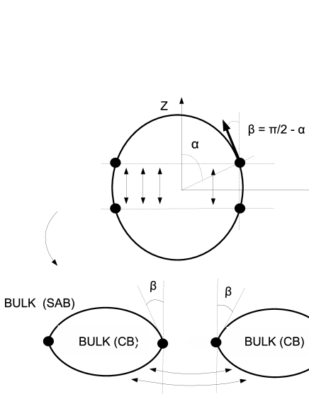
Figure 1: The brane trajectory in the $R-Z$ plane, for a generic DW in an inflating brane $(H\neq 0)$. The two figures represent a constant time snapshot, and one of the directions along the DW (represented by the thick dot) is obtained in the upper diagram by rotating it around the $Z$ (vertical) axis. The space is cut by the two constant $Z$ sections where the brane is at an angle $\alpha=H\xi_{0}$. The space in between is then removed, and the two slices joined together. Then, another identical copy of the resulting ‘pancake’ is glued along the brane, as indicated in the lower diagram. For the conventional branch (CB), the bulk is the interior, while for the self-accelerated branch (SAB), it is the exterior. For the CB, this space has a deficit angle $\delta=4\beta$, with $\beta=\pi/2-\alpha$. For the SAB, we have an excess angle, that is $\delta=-4\beta$.

Assuming $Z_{2}$ symmetry across the wall Eq (3.17) reads, in terms of $\beta$,

$$2\kappa\,Hr_{c}\,{\tan\beta}+\epsilon\;\beta={\sigma\over 4M_{*}^{3}}~{}.$$ (3.18)

This equation cannot be solved analytically (except for $\kappa=0$), but it is straightforward to solve it numerically for given values of the parameters. We shall now do this in the next subsections.

For clarity, we shall now summarize the main features of these solutions. It is already apparent from (3.17) that both the 5D effect (amount of deficit angle) and the 4D effect (the jump within the brane induced metric) produced by the wall will in general differ from the usual pure 4D or 5D ones. In order to quantify these deviations we can always introduce the effective 4D and 5D tensions in terms of whichever geometrical effect is produced,

$$\sigma^{(4D)}_{\rm eff}\equiv-2\kappa\;m_{P}^{2}\;{\Delta R^{\prime}_{0}\over R_{0}}$$ (3.19)

and

$$\sigma^{(5D)}_{\rm eff}\equiv\delta\,M_{*}^{3}~{}.$$ (3.20)

Recalling that the deficit angle in (3.17) arises from the extrinsic curvature and that the jump in $R^{\prime}$ comes from the intrinsic curvature, we readily identify that $\sigma^{(4D,5D)}_{\rm eff}$ contain a contribution from $K_{\mu\nu}$ and from $G_{\mu\nu}$ respectively, aside from the DW tension itself. Also, in terms of $\sigma^{(4D,5D)}_{\rm eff}$, the wall junction condition (3.17) can be expressed as a ‘sum rule’,

$$\sigma^{(4D)}_{\rm eff}+\sigma^{(5D)}_{\rm eff}=\sigma~{}.$$ (3.21)

Note also that the notion of the 5D tension (3.20) is not valid for super-critical walls ($\sigma>2\pi M_{*}^{3}$), simply because the deficit angle cannot exceed $2\pi$ without adding extra sources. The appropriate notion in this case will require some previous familiarization with super-massive codimension-2 objects, and will be discussed at length in Section 3.3.

branch	DW tension	$\sigma^{(4D)}_{\rm eff}/\sigma$	$\sigma^{(5D)}_{\rm eff}/\sigma$
CB	$\sigma<2\pi M_{*}^{3}$	$0$	$1$
	$\sigma>2\pi M_{*}^{3}$	$\displaystyle 1-{2\pi M_{*}^{3}\over\sigma}$	$\displaystyle{d\over 2r_{c}}$
SAB	$\sigma\ll 2\pi M_{*}^{3}$	$\displaystyle 2\left(1-\left(\sigma/M_{*}^{3}\right)^{2}/48+\dots\right)$	$\displaystyle-\left(1-\left({\sigma/M_{*}^{3}}\right)^{2}/24+\dots\right)$
	$\sigma\gg 2\pi M_{*}^{3}$	$\displaystyle 1+{2\pi M_{*}^{3}\over\sigma}+\dots$	$\displaystyle-{d\over 2r_{c}}$

Table 1: Summary of the screening properties of our solutions. See the discussion in the text for the definitions of $\sigma^{(4D)}_{\rm eff}$ and $\sigma^{(5D)}_{\rm eff}$. Notice that for sub-critical walls, the sum rule (3.21) is satisfied.

Now, let us briefly go through the results displayed in Table 1. As mentioned in the introduction, in the Conventional Branch, sub-critical walls suffer a complete screening of their 4D tension. The wall effectively switches on the extrinsic curvature in such a way that it completely compensates for the wall tension. Let us emphasize that the 4D curvature of the brane is zero in this case even on the DW location. Precisely for this reason, the 5D tension is not screened at all.

Still for the Conventional Branch, the supercritical walls show a very different behaviour. First of all, the wall starts to inflate. So, the screening of the 4D tension is not total. At the same time, the 5D tension is screened by a huge factor. What happens in this case is that the space transverse to the wall is compactified to a size of the order of the thickness $d$ of the DW core (we are assuming that $d$ is finite but small, $d\ll r_{c}$). Hence, the model changes significantly, e.g., there exists a graviton zero mode. Nevertheless, as we shall show in Section 3.3, ‘ordinary’ super-massive codimension-2 objects (i.e., without the DGP brane) also compactify one direction of the transverse space, and start to inflate. Hence, the 5D effect to which we should compare is the worldvolume inflation rate, rather than the deficit angle (which is saturated to $2\pi$). As we shall see, the walls in a DGP brane inflate at a rate suppressed by $d/2r_{c}$ relative to the ones without the brane. As argued before, the analog of $r_{*}$ scale for for all kinds of walls coincides with the thickness $d$. Hence, quite surprisingly, the super-critical walls display the same screening of the 5D tension/mass found in [7] for the Schwarzchild-like objects.

In the SA branch, we will see that the deficit angle is negative, meaning that the 5D tension is ’over-screened’ (the sign of the net tension $\sigma^{(5D)}$ is reversed). On the other hand, from the 4D point of view, there is anti-screening: the extrinsic curvature takes the form of a positive tension wall. For small tensions, $K_{\mu\nu}$ mimics a wall with almost exactly the same tension, so the 4D effect is enhanced by a factor 2. In the super-critical case, we shall find a suppression of the Hubble rate on the wall $\sim d/2r_{c}$, while the deficit angle is close to $-2\pi$ instead of $2\pi$ (which is what the sign in the lower-right entry of Table 1 stands for).

3.1 Conventional Branch

This branch is defined by requiring that the brane extrinsic curvature be positive ($\epsilon=1$) for non-negative brane tension $\tau$. As seen from (3.16), this implies that a positive tension wall generates as usual a deficit angle in the bulk. From (3.17), we also see that this can be interpreted from the point of view of the brane as a screening due to the extrinsic curvature term, which behaves like a negative tension domain wall. As we will now see, the amount of screening depends on the brane tension, and in the extreme case $\tau=0$, there is complete screening.

Flat domain wall ($\kappa=0$)

In this case, Eq. (3.8) is automatically satisfied if we set $\tau=0$. On the other hand, Eq. (3.13) is of the form $R^{\prime\prime}\propto\sigma\delta(\xi)$. Hence, taking into account (3.7), the trajectory is of the form

$$R(\xi)=|\xi|\;\sin\beta\qquad\qquad Z(\xi)=\xi\;\cos\beta\;$$ (3.22)

The junction condition on the DW (3.17) fixes $\beta$, and leads to an expression for the deficit angle

$${\delta}={\sigma\over M^{3}_{*}}~{},$$

as for an ordinary codimension-2 object. This space is illustrated in Fig. 2. It makes sense as long as the deficit angle is less than $2\pi$, that is for

$$\sigma<2\pi M_{*}^{3}~{}.$$

We recognize that the linearized solution of Sec. 2 was tailored to reproduce this exact metric.

Figure 2: Conical space corresponding to the flat DW case in a flat brane. The deficit angle is $\delta=4\beta$, which is always less than $2\pi$. This figure refers to the Conventional Branch, and with zero brane tension.

Now that we have a geometrical method to find the solutions, we could easily construct multi-center solutions with as many DWs as we’d like. The induced metric is always trivial (up to the topology), and the embedding of the brane in the bulk has a kink-shape, as in Fig 2, at each DW. In particular, if the wall tensions add up to $2\pi$, then the bulk is compactified with compactification radius related to the separation between the walls.

Let us now describe in more detail the critical case, $\sum\sigma=2\pi M_{*}^{3}$. A single critical wall leads to a seemingly singular space because the angular component of the metric (2.7) vanishes. This is of course an artifact of the thin wall approximation. If we introduce the thickness of the wall $d$, then the metric asymptotes that of a cylinder of radius $d$. Hence, the bulk (the transverse space) is compactified, and in the ’thin wall’ limit $d\to 0$, one transverse direction disappears. We can illustrate these statements giving the critical wall some structure, for example by splitting it into two walls with tensions $3\pi/2$ and $\pi/2$ (in units of $M^{3}_{*}$), separated by a distance $d$. Since each of them is subcritical, the bulk is a wedge of $2\pi$ minus the deficit angle at each wall. In this case, instead of Fig 2, the bulk looks like (two copies of) a semi infinite strip of width $d$. Thus, the compactification radius coincides with the separation between walls.

This solution contains one modulus, $d$. At first, this is puzzling because it seems that it costs no energy to move the walls apart, but this would result in changing the compactification scale. The reason why there is no paradox is that to change globally the position of the walls actually costs an infinite amount of energy. The fact that $d$ is a flat direction means that local perturbations in the wall separation propagate as massless fields.

There appears to be another paradox, though: the bulk is compactified, so one expects to have four dimensional gravity at distances larger than $d$. However, the DW is flat, so it does not gravitate as in 4D. This situation occurs also in ordinary Kaluza-Klein theories, without the brane. A critical codimension-2 object in 5D compactifies one transverse in the same way, producing an effectively 4D space. But it does not inflate, as it would in 4D. This an example of off-loading: all the gravitational effect of the DW tension is ’exhausted’ in compactifying the transverse space. We will see below that if the tension is supercritical, then it starts behaving as in 4D, and in the limit $\sigma\gg M_{*}^{3}$ we will recover the usual metric of a domain wall on the brane. But in the critical case, the four dimensional behavior is not reproduced.

Finally, we shall mention that the space generated by a critical (distribution of) walls is unstable under nucleation of bubbles of nothing, very much like with the Kaluza-Klein vacuum [21]. The reason is that, the space is asymptotically cylindrical, which has the same topology as the bubble of nothing instanton. The estimated nucleation rate is of order $\exp(-m_{P}^{2}R^{2})$ [21], where $R$ is the (asymptotic) radius of the extra dimension. In our case, this is related to the wall thickness. For a single critical wall, assuming that its thickness is of the same order as the scale of the tension $M_{*}$, this gives a highly suppressed rate. For an extended distribution of walls $R$ is larger, so the rate is even more suppressed.

Inflating domain wall ($\kappa=1$)

Solving for $\beta$ in Eq. (3.18) for $\tau\neq 0$, we can find the deficit angle $\delta$ and the DW radius $R_{0}=H^{-1}\cos\beta$. The results are shown in Fig. 3 for $Hr_{c}=1/5$ and $1/100$. We can see how as $H\to 0$, the subcritical walls (with $\sigma<2\pi M_{*}^{3}$) are much flatter than in usual GR.

$$\begin{array}[]{cc}\includegraphics[width=170.71652pt]{R0_Z2_normal.eps}&\includegraphics[width=170.71652pt]{R0_Z2_normal2.eps}\\[14.22636pt] \includegraphics[width=170.71652pt]{R0_Z2_normal_H0.eps}&\includegraphics[width=170.71652pt]{delta_Z2_normal2.eps}\\[-14.22636pt] \end{array}$$

Figure 3: The radius of the DW $R_{0}$ for the conventional branch (CB), in the $Z_{2}$ symmetric case, for $Hr_{c}=0.2,0.01$ and $0$, and the deficit angle (for $Hr_{c}=0.01$) as a function of the tension $\sigma$. We see how the DW tension is screened by the $K_{\mu\nu}$ term (contributing effectively negative tension), so that the radius of the DW is larger than in 4D GR (dashed line). There is a qualitative change of behavior for tensions below or above the critical value $2\pi M_{*}^{3}$ (vertical lines). In the limit $H=0$, tensions smaller than or equal to $2\pi M_{*}^{3}$ induce a flat DW. Only for $\sigma>2\pi M_{*}^{3}$, the DW worldsheet is inflating, and $R_{0}$ approaches the 4D value ($r_{dw}$) for $\sigma\gg M_{*}^{3}$.

For $H=0$, Eq. (3.10) implies that $R^{\prime 2}=1$. Thus, the brane trajectory lies along $Z=const.$ lines in the $Z-R$ plane, which means that the deficit angle is $2\pi$ (for the CB). Strictly speaking, this limit is singular, because the bulk collapses to zero volume. However, if we introduced the DW thickness $d$, we would realize that the bulk is a slice of size roughly given by $d$. Here, we shall ignore these details and assume that the geometry is appropriately regularized in such a way that it still makes sense to speak of a deficit angle $2\pi$. Then, the matching condition (3.17) takes the following form,

$${1\over R_{0}}+\,{\pi\over 4r_{c}}={1\over r_{dw}}$$ (3.23)

The solutions of this equation are represented in the lower left plot of Fig 3. Solutions with a finite Hubble radius $R_{0}$ start to exist for supercritical walls $\sigma>{2\pi}M_{*}^{3}$. Subcritical walls have an infinite $R_{0}$, that is they are flat, in agreement with the arguments of the previous sections.

3.2 Self-accelerated branch

In this case, the brane extrinsic curvature is negative ($\epsilon=-1$). This implies that a positive tension wall generates a negative deficit angle in the bulk (see Fig 1, or Eq. (3.16)). From the point of view of the brane, this is seen as an anti-screening due to the extrinsic curvature term. Using e.g. (3.18) for $\tan\beta\simeq\beta\ll 1$, one obtains $\tan\beta\propto R^{\prime}_{0}/R_{0}$ twice as large as in GR. This means that in this case $K_{\mu\nu}$ behaves like a positive tension domain wall with effective tension $\sigma$.

From the point of view of the bulk, however, there is ‘over-screening’. Indeed, the deficit angle is negative (see Fig 4), which means that the effective codimension-2-tension is negative. This can also be visualized from Fig 1: for the SA branch, the bulk is the exterior of the brane, which gives an excess angle.

We can also see this from Eq (3.18) for small DW tension, $\sigma\ll M_{*}^{3}$. In this limit also $\beta\ll 1$, so the deficit angle is approximately (here we take $\kappa=1$)

$$\delta\simeq{1\over 1+2\epsilon Hr_{c}}\;{\sigma\over M_{*}^{3}}~{}.$$ (3.24)

Hence, in the CB there is screening, while on in the SAB there is ’over-screening’. In fact for the SAB with zero tension, the deficit angle is exactly opposite as the naively expected.

Two comments are now in order. Given that from the point of view of the bulk the wall in the SAB behaves as with negative tension, it appears that the stability of this solution is not granted. However, a perturbative analysis would not be conclusive, since the brane is in a strong coupling regime for this solution [22, 13]. On the other hand, it is clear that a perturbative treatment as in Section 2 will not capture the over-screening. This is precisely a consequence of the non-perturbative nature of the solution.

$$\begin{array}[]{ccc}\includegraphics[width=142.26378pt]{delta_Z2_self.eps}&\includegraphics[width=142.26378pt]{R0_Z2_self.eps}&\includegraphics[width=142.26378pt]{sigma4Dsigma.eps}\\[-14.22636pt] \end{array}$$

Figure 4: The deficit angle and the radius $R_{0}$ of the DW for the Self-Accelerated Branch. The radius $R_{0}$ approaches its 4D value (dashed line) for large $\sigma$. The fact that $R_{0}$ is smaller than the GR result is a consequence of the anti-screening produced by the extrinsic curvature term. In the third plot, we see the anti-screened the 4D tension, which amounts to a factor $2$ for small $\sigma$. For large tension, $\sigma^{(4D)}$ approaches the GR result.

3.3 Super-critical walls and screening of the 5D tension

In this section we discuss the spacetime produced by a (local) supermassive codimension-2 brane in ordinary gravity, in order to compare it to the supercritical walls found above. Solutions of a super-massive Abelian-Higgs vortex have been previously found numerically [23, 24]. The metric was shown to be regular and time-dependent, essentially because topological-inflation sets in.

In our case, the codimension-2 object is assumed to have the form of (thick) a Domain Wall confined on a ‘fake’ brane (with negligible tension and thickness, and no induced gravity term). As such, it does not have cylindrical symmetry. Rather, it is like a strip of a codimension-1 object of a finite extent, which, seen from afar appears as codimension-2. Thus, the problem under consideration is slightly different from that of [23, 24]. The advantage is that we can find the solution analytically, and the detailed structure of the core is not going to be important. Let us also emphasize that the solutions presented in this section are not the most general compatible with the assumed symmetries, since we will also require that the space outside the object is locally flat (this is a similar to the restriction to $C_{u}=0$, $u=1$ in (3.2)). We shall show that also these ordinary codimension-2 objects with tension $\sigma>2\pi M_{*}^{3}$, the worldsheet starts to inflate, and we shall compute at which rate.

We can proceed in the same way as in Section 3 with vanishing brane tension $\tau=0$. We shall concentrate on the five dimensional case, and take a generic form of the energy momentum tensor compatible with the symmetries of the wall,

$$T_{\mu}^{\nu}={\rm diag}(-\rho,-\rho,-\rho,P)~{},$$

and we assume that $\rho$ and $P$ (if nonzero) depend on $\xi$ only and are peaked around $\xi=0$. We shall not assume any particular microscopic model for the wall. Let us just mention that thick gravitating domain walls arising from scalar field models do develop a non-vanishing pressure in the core [25] (see also [26]).

The embedding equations (3.8) and (3.13) without the induced gravity term and with $\tau=0$ become

$$2\kappa\;M_{*}^{3}\;{\sqrt{1-R^{\prime 2}}\over R}=-{P\over 3}~{},$$ (3.25)

and

$$-2M_{*}^{3}\;{R^{\prime\prime}\over\sqrt{1-{R^{\prime}}^{2}}}=\left({2\over 3}P+\rho\right)~{},$$ (3.26)

which in fact is equivalent to (3.25) once the conservation equation

$$P^{\prime}+3\kappa\,{R^{\prime}\over R}\left(P+\rho\right)=0$$

is used.

Equation (3.25) immediately tells us that $P\leq 0$, and that it should vanish when the worldvolume does not inflate ($\kappa=0$). Instead, if it inflates, then $P$ is nonzero essentially at the location of the object, where $R^{\prime 2}\neq 1$.

As seen from (3.22), a subcritical wall produces a discontinuity $|\Delta R^{\prime}|<2$ while a critical wall saturates this bound. For supercritical walls, then there are two options: one is to have a larger $|\Delta R^{\prime}|$, but this would require another source at finite distance. The other is that the $P$ switches on. Let us now see that this is compatible with keeping $|\Delta R^{\prime}|=2$ for the supercritical walls. The integral of Eq. (3.26) around the core (that is from $R^{\prime}=1$ to $R^{\prime}=-1$) gives

$$2\pi M_{*}^{3}=\int d\xi\,(\rho+2P/3)~{}.$$

If we keep calling $\sigma\equiv\int_{core}\rho\,d\xi$ the tension, and defining the width of the wall $d$ by $\int_{core}Pd\xi\equiv P_{0}\,d$, we obtain

$$-{2\over 3}P_{0}\,d=\sigma-2\pi M_{*}^{3}~{},$$

where $P_{0}=P(0)$. Now, Eq. (3.25) tells us that at the center of the core ($R^{\prime}=0$) the Hubble rate $1/R_{0}$ is related to $P_{0}$ as

$$-P_{0}={6M_{*}^{3}\over R_{0}}$$

we arrive at

$${1\over R_{0}}={1\over 4dM_{*}^{3}}\left(\sigma-2\pi M_{*}^{3}\right)~{}.$$ (3.27)

Given that $R^{\prime 2}=1$ outside the walls the transverse space is compactified to a length equal to the thickness $d$. Hence, the theory becomes effectively 4-dimensional, with an effective 4D Planck mass

$$M_{4}^{2}=M_{*}^{3}\,d~{}.$$

With this in mind, we can rewrite (3.27) as

$${1\over R_{0}}={\sigma\over 4M_{4}^{2}}-{\pi\over 2d}~{}.$$ (3.28)

Hence, we see that we obtained the expected results: Eq (3.27) tells us that for tension larger than $2\pi M_{*}^{3}$, the wall starts to inflate; The Hubble rate approaches that of a codimension-1 object in GR (in terms of the effective Planck mass $M_{4}$). The interpretation of (3.28) in 4D terms is also interesting: the 4D tension of the wall is screened by the higher dimensional effects by an effective mirror wall with negative tension and an equivalent horizon of order $d$.

It is also worth describing the structure of the space-time generated by this object. The space is (the interior of) a flat ‘pancake’ of a thickness essentially given by the thickness of the wall, $d$. Hence, the picture is similar to Fig. 1, but with the ‘sides’ completely flat. The finite expansion rate on the wall translates into the fact that the object is placed at a finite radial distance $R$ (recall that in Fig 1, the horizontal coordinate is a radial Rindler coordinate). Accordingly, the presence of a horizon at a finite distance from the object is seen in the picture because the coordinate orthogonal to the object ‘terminates’ at the origin $R=0$ (which is actually the horizon).

Now that we know how supermassive codimension-2 objects behave, we can compare to what we found for the DGP model. Note that (3.28) is very similar to (3.23) with the thickness $d$ instead of $2r_{c}$ and $M_{4}$ instead of $m_{P}$ (the coefficient in the induced gravity term). One immediately realizes that the Hubble rates induced on the objects in DGP is extremely suppressed as compared to ordinary 5D gravity,

$${1/R_{0}^{(DGP)}\over 1/R_{0}^{(5D)}}={d\over 2r_{c}}~{}.$$ (3.29)

Hence, the 5D tension is suppressed by a factor $d/r_{c}$, which as argued before is the same as $r_{*}/r_{c}$, since the scale where the nonlinearities build up is $r_{*}=d$ for domain walls. Note that this is exactly the same suppression that occurred in the Schwarzchild solution found in [7], which also applies to the supercritical case where the radius of the source is less than its own $r_{*}$. Note also that for the domain walls, the 4D tension is screened, even though not completely. Indeed, without screening of the 4D tension one would expect $1/R_{0}=\sigma/4m_{P}^{2}$ and instead one has (see (3.23))

$${1\over R_{0}}={\sigma\over 4m_{P}^{2}}-{\pi\over 4r_{c}}~{}.$$

At this point, it might seem that the screening of the 5D tension (3.29) for super-critical walls is suspiciously discontinuous: in the 5D limit, $r_{c}\to 0$, (3.29) should go to $1$. Let us now show that this is precisely what happens, once we include the thickness of the wall from the beginning when the wall is on a DGP brane. We only need to repeat the above steps keeping the induced gravity terms. The junction equations are

$$2\epsilon\;M_{*}^{3}\;{\sqrt{1-R^{\prime 2}}\over R}=-\;m_{P}^{2}\;{1-R^{\prime 2}\over R^{2}}\;-{P\over 3}~{},$$ (3.30)

and

$$-2\epsilon M_{*}^{3}\;{R^{\prime\prime}\over\sqrt{1-{R^{\prime}}^{2}}}=2\;m_{P}^{2}\;{R^{\prime\prime}\over R}+\left({2\over 3}P+\rho\right)~{}.$$ (3.31)

On one hand, we can read from (3.30) that

$$-{P_{0}\over 3}=\left({2\epsilon\,M_{*}^{3}\over R_{0}}+{m_{P}^{2}\over R_{0}^{2}}\right)~{}.$$ (3.32)

Integrating this equation along the core of the wall, we obtain, for the Conventional Branch,

$$2\pi\,M_{*}^{3}={2\over 3}d\,P_{0}+\sigma-4m_{P}^{2}\,{1\over R_{0}}~{}.$$ (3.33)

From this and (3.32), we arrive at

$$4{m_{P}^{2}+d\,M_{*}^{3}\over R_{0}}+2{m_{P}^{2}\,d\over R_{0}^{2}}=\sigma-2\pi\,M_{*}^{3}~{}.$$ (3.34)

Assuming that $d\ll r_{c}$, one sees that the for $R_{0}\gg d$ the $1/R_{0}$ term dominates. Hence, we obtain

$${1\over R_{0}}={1\over 4}\,{\sigma-2\pi\,M_{*}^{3}\over m_{P}^{2}+d\,M_{*}^{3}},$$ (3.35)

which gives the suppression factor

$${d\over d+2r_{c}}\simeq{d\over 2r_{c}}~{}.$$ (3.36)

Note that (3.35) being consistent with our assumption that $R_{0}\gg d$ leads to

$$d\ll{8\over\pi}{1\over{\sigma\over 2\pi M_{*}^{3}}-1}\;r_{c}~{}.$$ (3.37)

This, though, does not seem to be much of a constraint for microscopic walls unless the tension is extremely large.

For the SAB, (3.33) reads

$$-4\arccos(R_{0}^{2}/r_{c}^{2})\,\;M_{*}^{3}={2\over 3}d\,P_{0}+\sigma+4m_{P}^{2}\,{1\over R_{0}}$$ (3.38)

so the analog of (3.34)

$$4m_{P}^{2}{1-d/2r_{c}\over R_{0}}+2{m_{P}^{2}\,d\over R_{0}^{2}}=\sigma+4M_{*}^{3}\,\arccos(R_{0}^{2}/r_{c}^{2})~{}.$$ (3.39)

Again, assuming that $d\ll r_{c}$ one obtains for $d\ll R_{0}\ll r_{c}$,

$${1\over R_{0}}={\sigma+2\pi M_{*}^{3}\over 4(1-d/2r_{c})m_{P}^{2}}~{},$$ (3.40)

leading to the suppression factor

$${\sigma+2\pi M_{*}^{3}\over\sigma-2\pi M_{*}^{3}}{d\over 2r_{c}-d}~{},$$

which, for $\sigma\gg M_{*}^{3}$ coincides with the one for the CB, (3.36). Also, the consistency of (3.40) with the approximation $d\ll R_{0}\ll r_{c}$ leads to a mild condition similar to (3.37).

4 Domain walls in IR modified gravity

Our findings of the previous section may well hold in more general models of modified gravity. Detailed arguments in favor of this will be discussed below. However, before we plunge into those considerations we’d like to emphasize the following: Nonlinear effects played an important role in the previous section where we obtained the results in DGP. Unfortunately, it is not clear whether the general models which we will discuss below have any consistent nonlinear counterparts. For one, massive gravity is known not to have a consistent nonlinear completion [27, 28, 29], as any of its versions gives rise to certain ghost-like instabilities. All of our discussions concerning general models below ignore these difficulties, and we have no way of assessing at present the significance of this for our discussions.

The most general ghost-free linearized theory in which gravity is mediated by a symmetric tensor field $h_{\mu\nu}$, is a generalization of the Fierz-Pauli [30] massive theory, and satisfies the following equation [13],

$$\mathcal{E}^{\alpha\beta}_{\mu\nu}h_{\alpha\beta}\,\,-\,m^{2}(\square)\,(h_{\mu\nu}\,-\,\eta_{\mu\nu}h)\,=\,-16\pi G_{N}\;T_{\mu\nu}~{},$$ (4.1)

where,

$$\mathcal{E}^{\alpha\beta}_{\mu\nu}h_{\alpha\beta}\,=\,\square h_{\mu\nu}\,-\,\square\eta_{\mu\nu}h\,-\,\partial^{\alpha}\partial_{\mu}h_{\alpha\nu}\,-\,\partial^{\alpha}\partial_{\nu}h_{\alpha\mu}\,+\,\eta_{\mu\nu}\partial^{\alpha}\partial^{\beta}h_{\alpha\beta}\,+\,\partial_{\mu}\partial_{\nu}h~{},$$ (4.2)

$h\equiv h_{\mu}^{\mu}$ and $G_{N}$ stands for the Newton’s constant.

For $m^{2}(\Box)=0$ this reduces to the linearized Einstein’s equations, describing the propagation of two polarizations of a massless spin-2 graviton. Here, we shall be interested mostly in the case $m^{2}(\Box)=const$, that corresponds to massive gravity; we will compare the latter to $m^{2}(\Box)=\sqrt{\Box}/r_{c}$, which corresponds to the DGP model. Our conclusions also apply to the more general cases where

$$m^{2}(\Box)=r_{c}^{-2(1-\alpha)}\Box^{\alpha}~{},$$ (4.3)

with $0\leq\alpha<1$ (the lower bound arising from unitarity [13]), assuming that these models have sensible nonlinear completions.

Gravitons satisfying (4.1) propagate 5 polarizations for nonzero $m^{2}(\Box)$, which is at the root of the vDVZ discontinuity [2]. The naive linearized metric produced by a localized source $T_{\mu\nu}$ is given by

$$h_{\mu\nu}=-16\pi G_{N}{1\over\Box-m^{2}(\Box)}\left\{T_{\mu\nu}-{1\over 3}\left(\eta_{\mu\nu}-{1\over m^{2}(\Box)}\partial_{\mu}\partial_{\nu}\right)T\right\}~{},$$ (4.4)

where $T\equiv T_{\mu}^{\mu}$. The factor $1/3$ reflects the existence of the extra helicity-0 polarization $\chi$, residing in $h_{\mu\nu}$. The latter could be separated as follows:

$$h_{\mu\nu}=\tilde{h}_{\mu\nu}+{1\over 6}\eta_{\mu\nu}\,\chi+{1\over 3}{\partial_{\mu}\partial_{\nu}\over m^{2}(\Box)}\,\chi~{},$$ (4.5)

where $\tilde{h}_{\mu\nu}$ contains the usual 2 polarizations, as in the massless case, and the helicity-1 states are ignored as they do not couple to conserved sources in the linearized theory. Convoluting Eq. (4.4) with a stress-tensor of a test source $T^{\prime}_{\mu\nu}$, we obtain the following one-graviton exchange amplitude

$${\cal A}\;\propto\;G_{N}\int d^{4}x\;{T_{\mu\nu}T^{\prime\mu\nu}-{1\over 3}TT^{\prime}\over\Box-m^{2}(\Box)}~{}.$$

Let us apply this to an infinite domain wall with the stress-tensor given in (1.1). Taking a non-relativistic probe $T^{\prime}_{\mu\nu}=M\,\delta_{\mu}^{0}\delta_{\nu}^{0}\,\delta^{(3)}(r)$, we obtain that the amplitude equals to zero! Actually, it is also easy to see that it vanishes for any conserved source. First, note that for the DW, the tensorial structure $T_{\mu\nu}-(1/3)T\eta_{\mu\nu}\propto\delta_{\mu}^{z}\delta_{\nu}^{z}$. Hence, the amplitude is

$$\int d^{4}x\;T^{\prime}_{zz}f(z)=-\int d^{4}x\;\partial^{z}T^{\prime}_{zz}\int^{z}dz^{\prime}f(z^{\prime})=\int d^{4}x\;\partial^{A}T^{\prime}_{Az}\int^{z}dz^{\prime}f(z^{\prime})=0~{},$$

where $f(z)$ is the result of applying $(\Box-m^{2}(\Box))^{-1}$ on $\delta(z)$ (certainly a function of $z$ only). In the derivation above, we integrated by parts, used the local conservation of $T^{\prime}_{\mu\nu}$, and integrated by parts again (the label $A$ stands for all coordinates except $z$). Hence, we conclude that the amplitude vanishes, which is due to the ‘pure gauge’ form of the metric (4.4) for the DWs.

Thus, in the naive linearized approximation, domain walls in massive gravity (and in general theories parameterized by (4.3)) do not gravitate. This conclusion, however, is not warranted until the nonlinear effects are taken into account. This is because of two interrelated reasons already discussed in Sections 1 and 2: (1) There is an ambiguity in linearized solutions; one cannot decide whether to choose a time-dependent or a static solution, without knowing what is going on with the source itself. (2) In modified gravity, non-linearities introduce a scale $r_{*}$ at which the perturbative expansion breaks down, and, therefore at $r\mathrel{\hbox to0.0pt{\lower 3.0pt\hbox{\hskip 0.0pt$\sim$}\hss}\raise 1.0pt\hbox{$<$}}r_{*}$ the above results cannot be applied. In DGP these issues were addressed by finding exact nonlinear solutions in Section 3. We do not have the luxury of a stable nonlinear theory in the case of massive gravity (and the general $\alpha$-theories (4.3)). However, this may only be a temporary technical problem, and if so, it would make sense to try and estimate what the analog of the $r_{*}$ scale for a domain wall in massive gravity is. We will do this below.

First we recall that the $r_{*}$ scale and strong coupling originates from the $1/m^{2}(\Box)$ term in (4.4), which at the non-linear level gives rise to interactions that become singular for $m^{2}(\Box)\to 0$ [3]. In a schematic way, the leading singular vertex has the form [13]

$$r_{c}^{4(1-\alpha)}{\partial^{4}\over\Box^{2\alpha}}\;\chi\;(\partial\chi)^{2}~{},$$ (4.6)

where we should keep in mind that the four derivatives do not necessarily come in the form of $\Box^{2}$. For $\alpha=0,1/2$, this was found in [3] (see also [31] for $\alpha=0$). Due to this singularity, the localized gravitating sources end up having a new ‘horizon’ at $r=r_{*}$, where the perturbative expansion in $G_{N}$ breaks down. Consider now a non-relativistic spherically symmetric source $T_{\mu\nu}=M\,\delta_{\mu}^{0}\delta_{\nu}^{0}\,\delta^{(3)}(r)$, with a gravitational radius $r_{g}=2G_{N}M$. The scale $r_{*}$ is then found as follows: Assume that far enough from the source, the linearized solution

$$h_{\mu\nu}=-{\delta_{\mu}^{0}\delta_{\nu}^{0}-{1\over 3}\left(\eta_{\mu\nu}-{\partial_{\mu}\partial_{\mu}\over m^{2}(\Box)}\right)\over\Box-m^{2}(\Box)}\,8\pi\,r_{g}\,\delta^{3}(r)$$ (4.7)

is valid. From this and (4.5), one finds that for $r\ll r_{c}$

$$\chi\simeq{1\over 2}\,{r_{g}\over r}~{}.$$ (4.8)

At the scale $r_{*}$ the contributions from the nonlinear diagrams (4.6) catch-up with the leading linear one. This happens when

$$\left({r_{c}\over r}\right)^{4(1-\alpha)}{r_{g}\over r}\sim 1~{}.$$

This determines the Vainshtein scale [32]

$$r_{V}\sim\left(r_{g}m^{-4}\right)^{1/5}\,,$$ (4.9)

for massive gravity, and the $r_{*}$ scale

$$r_{*}\sim\left(r_{g}r_{c}^{2}\right)^{1/3}\,,$$ (4.10)

for DGP. At $r\mathrel{\hbox to0.0pt{\lower 3.0pt\hbox{\hskip 0.0pt$\sim$}\hss}\raise 1.0pt\hbox{$<$}}r_{*}$, the metric can be found as a series in $r/r_{c}$ [4].

Let us now apply similar considerations to subcritical domain walls. Assuming that the linearized solution

$$h_{\mu\nu}=-{\delta_{\mu}^{z}\delta_{\nu}^{z}+{\partial_{\mu}\partial_{\nu}\over 3m^{2}(\Box)}\over\Box-m^{2}(\Box)}\;16\pi\,\sigma G_{N}\,\delta(z)~{},$$ (4.11)

is valid far-away from the source, for $z\ll r_{c}$ Eq. (4.11) leads to

$$\chi=-8\pi\,G_{N}\sigma\;|z|.$$

With such a dependence on $z$ the nonlinearities vanish due to the structure of the vertices. This is obvious for the leading singular vertex (4.6), and is also true for all the other interactions. The key point is that both for $m^{2}=const$ and for $m^{2}(\Box)=\sqrt{\Box}/r_{c}$, all non-linear vertices include at least one $\chi$ (or $h_{\mu\nu}$) with at least two derivatives. As a result, for solutions for which $h_{\mu\nu}$ is linear in $z$, the strongly coupled vertices vanish outside of the source. The only place where they can make contributions is in the core of the source itself. Thus, the scale $r_{*}$, for a subcritical domain wall, is determined by the transverse size of the wall itself. This is reminiscent of a metric of a subcritical Schwarschild source [7], except that the subcriticality condition in the two cases are quantitatively different.

Finally, let us discuss a similar issue for a wall with a finite longitudinal extent. Specifically, consider a disk of radius $L$ located on the plane $z=0$, and let us measure the gravitational interaction of this ‘wall’ along the $z$ axis. For $r_{*}\ll z\ll L$, the solution should be well approximated by (4.11), and $\chi\propto|z|$ as before. In this case, we could apply the same reasoning for strong coupling vertices as we did for an infinite wall, and could conclude that they vanish outside the wall as long as $r_{*}$ is smaller than $L$. Let us get a naive estimate for the value of $r_{*}$ for a finite wall. The total ‘mass’ of the source is (here we ignore the fact that the domain wall also has a negative pressure)

$$M\sim\pi\sigma L^{2}\sim\pi\delta M_{*}^{3}L^{2}~{},$$

where we introduced $\delta\equiv\sigma/M^{3}_{*}$, and $M_{*}$ is the fundamental Planck scale in the bulk (let us concentrate on the DGP model for the moment). Then the naive estimate $r_{*}^{naive}\sim(2G_{N}Mr_{c}^{2})^{1/3}$ would suggest

$$r_{*}^{naive}\sim\left(\delta L^{2}r_{c}\right)^{1/3}~{}.$$

If $r_{*}^{naive}$ is smaller than $L$, then non-linearities never contribute outside the wall. This gives the following constraint on the size of the wall

$$L\gg\delta\,r_{c}~{}.$$ (4.12)

Hence, in order to avoid the strong coupling of the longitudinal mode $\chi$, the wall radius has to be quite large; for $\delta\sim 1$ it should be larger than $r_{c}$. This is consistent with the expectation that the behavior of a DW here is different from that in GR. The above follows from the fact that the infinite domain wall is already probing the scale of modification of gravity $r_{c}$.

References

- [1] G. Dvali, G. Gabadadze and M. Porrati, Phys. Lett. B 485, 208 (2000).
-
[2]
H. van Dam and M. J. G. Veltman,
Nucl. Phys. B 22, 397 (1970).
V. I. Zakharov, JETP Lett. 12 (1970) 312 [Pisma Zh. Eksp. Teor. Fiz. 12 (1970) 447]. - [3] C. Deffayet, G. R. Dvali, G. Gabadadze and A. I. Vainshtein, Phys. Rev. D 65, 044026 (2002) [arXiv:hep-th/0106001].
- [4] A. Gruzinov, New Astron. 10, 311 (2005) [arXiv:astro-ph/0112246].
-
[5]
G. Dvali, A. Gruzinov and M. Zaldarriaga,
Phys. Rev. D 68, 024012 (2003)
[arXiv:hep-ph/0212069];
G. Dvali, arXiv:hep-th/0402130. - [6] T. Tanaka, Phys. Rev. D 69, 024001 (2004) [arXiv:gr-qc/0305031].
- [7] G. Gabadadze and A. Iglesias, Phys. Rev. D 72, 084024 (2005) [arXiv:hep-th/0407049]; Phys. Lett. B 632, 617 (2006) [arXiv:hep-th/0508201]; Phys. Lett. B 639, 88 (2006) [arXiv:hep-th/0603199].
- [8] A. Lue and G. Starkman, Phys. Rev. D 67, 064002 (2003) [arXiv:astro-ph/0212083].
- [9] L. Iorio, JCAP 0509, 006 (2005) [arXiv:gr-qc/0508047].
- [10] T.W. Murphy, Jr., E.G. Adelberger, J.D. Strasburg and C.W. Stubbs, ‘APOLLO: Multiplexed Lunar Laser Ranging’, at http://physics.ucsd.edu/tmurphy/apollo/doc/multiplex.pdf
- [11] A. Vilenkin, Phys. Lett. B 133 (1983) 177.
- [12] J. Ipser and P. Sikivie, Phys. Rev. D 30, 712 (1984).
- [13] G. Dvali, arXiv:hep-th/0610013.
- [14] A. Vilenkin, Phys. Rev. D 23 (1981) 852.
- [15] R. Gregory and A. Padilla, Phys. Rev. D 65, 084013 (2002) [arXiv:hep-th/0104262]; Class. Quant. Grav. 19, 279 (2002) [arXiv:hep-th/0107108].
- [16] S. Perlmutter et al. [Supernova Cosmology Project Collaboration], Astrophys. J. 517, 565 (1999).
- [17] A. G. Riess et al. [Supernova Search Team Collaboration], Astron. J. 116, 1009 (1998); Astrophys. J. 607, 665 (2004).
- [18] C. Deffayet, Phys. Lett. B 502, 199 (2001).
- [19] C. Deffayet, G. R. Dvali and G. Gabadadze, Phys. Rev. D 65, 044023 (2002) [arXiv:astro-ph/0105068].
- [20] In preparation.
- [21] E. Witten, Nucl. Phys. B 195, 481 (1982).
- [22] C. Deffayet, G. Gabadadze and A. Iglesias, JCAP 0608, 012 (2006) [arXiv:hep-th/0607099].
- [23] A. A. de Laix, M. Trodden and T. Vachaspati, Phys. Rev. D 57, 7186 (1998) [arXiv:gr-qc/9801016].
- [24] I. Cho, Phys. Rev. D 58, 103509 (1998) [arXiv:gr-qc/9804086].
- [25] L. M. Widrow, Phys. Rev. D 39, 3571 (1989).
- [26] A. z. Wang, Phys. Rev. D 66, 024024 (2002) [arXiv:hep-th/0201051].
- [27] D. G. Boulware and S. Deser, Phys. Rev. D 6, 3368 (1972).
- [28] G. Gabadadze and A. Gruzinov, Phys. Rev. D 72, 124007 (2005) [arXiv:hep-th/0312074].
- [29] C. Deffayet and J. W. Rombouts, Phys. Rev. D 72, 044003 (2005) [arXiv:gr-qc/0505134].
- [30] M. Fierz and W. Pauli, Proc. Roy. Soc. Lond. A 173 (1939) 211.
- [31] N. Arkani-Hamed, H. Georgi and M. D. Schwartz, Annals Phys. 305, 96 (2003) [arXiv:hep-th/0210184].
- [32] A. I. Vainshtein, Phys. Lett. 39B, 393 (1972).