Reconstructing 1/2 BPS Space-Time Metrics from Matrix Models and Spin Chains

Abstract

Using the AdS/CFT correspondence, we address the question of how to measure complicated space-time metrics using gauge theory probes. In particular, we consider the case of the 1/2 BPS geometries of type IIB supergravity. These geometries are classified by certain “droplets” in a two dimensional space-like hypersurface. We show how to reconstruct the full metric inside these droplets using the one-loop ${\cal N}=4$ SYM theory dilatation operator. This is done by considering long operators in the $SU(2)$ sector, which are dual to fast rotating strings on the droplets. We develop new powerful techniques for large $N$ complex matrix models that allow us to construct the Hamiltonian for these strings. We find that the Hamiltonian can be mapped to a “dynamical” spin chain. That is, the length of the chain is not fixed. Moreover, all of these spin chains can be explicitly constructed using an interesting algebra which is derived from the matrix model. Our techniques work for general droplet configurations. As an example, we study a single elliptical droplet and the “Hypotrochoid”.

I Introduction

One of the most striking predictions of the AdS/CFT correspondence, is the emergence of space-time geometry from the large $N$ limit of non-abelian gauge theories. The best understood example is the duality between ${\cal N}=4$ SYM theory on $\mathbb{R}\times S^{3}$ and type IIB String Theory on asymptotically $AdS_{5}\times S^{5}$ space-times malda .

It was understood early on, that the ground state of ${\cal N}=4$ SYM was dual to $AdS_{5}\times S^{5}$ itself. This matching was originally guessed based on the symmetries of the ground state. However, it was latter understood that one can also consider states dual to fast rotating strings on this background BMN . These states allowed a matching of the string spectrum, including the sigma model, in the appropriate limits Kruczenski . (See Tseytlinrev for a review and more references.) By matching the sigma-model of these strings one is also measuring the space-time metric of $AdS_{5}\times S^{5}$.

More recently, it has been possible to identify space-times that are dual to “heavy” 1/2 BPS states of the gauge theory LLM . These geometries have complicated metrics and topologies. Nevertheless, it was shown in LLM that they are classified in terms of “droplets” in a plane. Remarkably, the 1/2 BPS states of SYM are classified in exactly the same way toy ; matrixmaps .

Space-times corresponding to 1/4 and 1/8 BPS states have also been studied in 148bps . Their classification in terms of gauge theory operators is not completely understood, but some proposals have been put forward davidN ; Ryzhov .

In this paper, we address the question of how to measure the complicated metrics of the 1/2 BPS geometries using only gauge theory probes. To simplify the problem we focus on the $SU(2)$ sector of the gauge theory. As we explain below, this sector correspond to strings that live inside the “droplets” and rotate along an $S^{1}$ fiber. As usual, one can match a one-loop gauge theory calculation by studying strings with large angular momentum along this circle.

On the gauge theory side, the $SU(2)$ dilatation operator can be described by a model of matrix quantum mechanics with two matrices beisert . Using this model, we explain how one can excite a “heavy” 1/2 BPS state, and then put a probe string on it. The reduced Hamiltonian for the probe string can be computed using Random Matrix Theory techniques. Some of these techniques are developed here for the first time.

We find that the Hamiltonian of the probe string can be described by a bosonic lattice. This model has the usual hopping terms, but also include sources and sinks of bosons at each site. Alternatively, one can visualize the lattice as a “dynamical” spin chain. As it turns out, this Hamiltonian is completely determined by a very interesting algebra underlying the Random Matrix Model. Using coherent states, one can match the thermodynamic limit of this lattice to the sigma model of the fast string. This is how we measure the metric.

The techniques developed here are valid for any droplet configuration, including the case of multiple-connected domains. As an example, we study a single elliptical droplet, and the so-called “Hypotrochoid”.

The paper is organized as follows. In section II we review the 1/2 BPS geometries and set up the basic notation. In section III, we study the fast rotating strings. We derive their sigma-model for a general droplet configuration. We then specialize to the case of a single elliptical droplet, and the Hypotrochoid. In section IV we derive some general results for the gauge theory. We start with a review of the $SU(2)$ sector in order to set up notation. We then define the Hilbert Space for a probe string around an arbitrary 1/2 BPS background. Next, we derive the corresponding Hamiltonian using the one-loop dilatation operator. Coherent states are defined, and an effective sigma model is derived. At this stage, we show that the general form of the sigma model is exactly the same as the one found in the String Theory calculation. This allows the full metric on the droplet to be defined in terms of gauge theory quantities.

In sections V and VI, we consider the particular examples of the elliptical droplet and the Hypotrochoid, this time from the gauge theory side. We reproduce all String Theory results.

We conclude in section VI with a discussion which includes topics such as integrability, the prospect of probing Black Hole states, and extension of this procedure to other sectors of the gauge theory.

The reader familiar with Normal Random Matrices will find that this paper is basically an extension of these techniques to large $N$ complex ensembles.

II 1/2 BPS Metrics

All 1/2 BPS solutions to type IIB supergravity with $N$ units of RR five-form flux have been found in LLM . They preserve a bosonic $\mathbb{R}\times SO(4)\times SO(4)$ symmetry of the ten dimensional space-time. All solutions are classified by a single function, which we call $\rho$, on a two dimensional plane. The metrics can be written as,

$$ds^{2} = -h^{-2}(Dt)^{2}+h^{2}(dy^{2}+dzd\bar{z})+ye^{-G}d\Omega_{3}^{2}$$

$$+ye^{G}d\widetilde{\Omega}_{3}^{2},$$

$$h^{-2} = 2y\cosh G,$$

$$f = \frac{1}{2}\tanh G,$$

$$f(z,\bar{z},y) = -\frac{y^{2}}{2}\int d^{2}z^{\prime}\frac{\rho(z^{\prime},\bar{z}^{\prime})}{(|z-z^{\prime}|^{2}+y^{2})^{2}}.$$ (1)

Here, we have defined the covariant derivative, $Dt=dt+V=dt-\frac{1}{2}i\bar{V}dz+\frac{1}{2}i{V}d\bar{z}$, and we are using complex coordinates in the $y=0$ plane: $z=x_{1}+ix_{2},\bar{z}=x_{1}-ix_{2}$. Moreover,

$$V(z,\bar{z},y)=-V_{2}+iV_{1}=\frac{1}{2}\int d^{2}z^{\prime}\frac{\rho(z^{\prime},\bar{z}^{\prime})(z-z^{\prime})}{(|z-z^{\prime}|^{2}+y^{2})^{2}}\;.$$ (2)

All non-singular solutions must have $\rho=\pm 1/\pi$. Therefore we can separate the integrations above in domains or “droplets” (${\cal D}_{i}$) for which $\rho=1/\pi$ (say) inside and $\rho=-1/\pi$ outside. These are the configurations that we will consider in this paper.

The size of the asymptotic $AdS_{5}\times S^{5}$ is set by LLM ,

$$R_{AdS_{5}}^{4}=R_{S^{5}}^{4}=\sum_{i}\int_{{\cal D}_{i}}d^{2}z\rho(z,\bar{z})\;.$$ (3)

Therefore, we can rescale all spatial coordinates by $x^{i}\rightarrow R^{2}_{AdS}x^{i}$ and we get an overall factor of $R_{AdS}^{2}$ in front of the metric. Then, our area quantization condition is simply, $\sum_{i}\int_{{\cal D}_{i}}d^{2}z\rho=1$. This makes it easier to compare with the gauge theory.

For a single simply connected domain $\cal D$, we can rewrite the integrals over the droplet as contour integrals over its boundary. We have,

$$V = \frac{1}{2}\int_{\cal D}\frac{d^{2}z^{\prime}}{\pi}\bar{\partial}^{\prime}\frac{1}{|z-z^{\prime}|^{2}+y^{2}}$$ (4)

$$-\frac{1}{2}\int_{\mathbb{C}\backslash{\cal D}}\frac{d^{2}z^{\prime}}{\pi}\bar{\partial}^{\prime}\frac{1}{|z-z^{\prime}|^{2}+y^{2}}$$

$$= \oint_{\partial D}\frac{dz^{\prime}}{2\pi i}\frac{1}{|z-z^{\prime}|^{2}+y^{2}}\;.$$

Similarly,

$$f = -\frac{1}{2}\int_{\cal D}\frac{d^{2}z^{\prime}}{\pi}\bar{\partial}^{\prime}\partial^{\prime}\log\left(|z-z^{\prime}|^{2}+y^{2}\right)$$ (5)

$$+\frac{1}{2}\int_{\mathbb{C}\backslash\cal D}\frac{d^{2}z^{\prime}}{\pi}\bar{\partial}^{\prime}\partial^{\prime}\log\left(|z-z^{\prime}|^{2}+y^{2}\right)$$

$$= \frac{1}{2}-\oint_{\partial D}\frac{dz^{\prime}}{2\pi i}\frac{\bar{z}^{\prime}-\bar{z}}{|z-z^{\prime}|^{2}+y^{2}}\;.$$

The factor of $1/2$ in $f$ comes from the boundary at infinity, and the contour integrals are taken counterclockwise.

This procedure is valid even for multiple droplets or non-simply connected domains. One obtains a superposition of contour integrals over the different boundaries of the domains. The orientation of the contours is such that we keep the regions with $\rho=1/\pi$ (the area of ${\cal D}_{i}$) to our left. These contour integrals can be solved, in general, by a conformal map from the boundaries to the unit circle. The problem then reduces to holomorphic contour integrals. We will illustrate this in the next section.

III Semiclassical Strings in the $SU(2)$ Sector

The $SO(4)$ subgroups in the isometry group of the 1/2 BPS geometries, correspond to rotations on the two $S^{3}$s that appear in the metric (II). In particular, one can see that in the asymptotic region, $\widetilde{S}^{3}\subset AdS_{5}$ and $S^{3}\subset S^{5}$. Inside each droplet ($y=0$), the size of $\widetilde{S}^{3}$ is zero.

The $SU(2)$ sector of the gauge theory consist of states with two R-charges. These two charges are identified (asymptotically) by a rotation along $S^{1}\subset S^{3}$, and a rotation around the origin in the $y=0$ plane. Therefore, one expects that the strings dual to these operators will “live” inside each droplet, and will rotate along an $S^{1}$ fiber.

The metric restricted to this subspace can be calculated by setting $y\rightarrow 0$ in (II) and restricting $z,\bar{z}$ inside the droplet. A careful calculation shows that,

$$\left.ds^{2}\right|_{SU(2)}=-h^{-2}(Dt)^{2}+h^{2}dzd\bar{z}+h^{-2}d\varphi^{2}\;,$$ (6)

where, for a single droplet,

$$h^{4} = \oint_{\partial D}\frac{dz^{\prime}}{2\pi i}\frac{\bar{z}^{\prime}-\bar{z}}{|z-z^{\prime}|^{4}}\;,$$ (7)

$$V = \oint_{\partial D}\frac{dz^{\prime}}{2\pi i}\frac{1}{|z-z^{\prime}|^{2}}\;.$$ (8)

This result can be generalized to the case of multiple droplets and for non-simply connected domains. One just needs to superimpose integrations over the different boundaries with the appropriate orientations. The important point to notice is that, in general, we can write,

$$V=\bar{\partial}\log K\;,\;\;\;h^{4}=\partial V=\partial\bar{\partial}\log K\;,$$ (9)

where we define,

$$\log K\equiv\sum_{i}\oint_{\partial D_{i}}\frac{dz^{\prime}}{2\pi i}\frac{1}{z-z^{\prime}}\log(\bar{z}-\bar{z}^{\prime})\;.$$ (10)

As we will see, the “Kähler potential” $K$ will have a very special interpretation as a sum of orthogonal polynomials.

Let us now look at the fast string limit along $\varphi$. As usual kru , we start with the Polyakov action in momentum space,

$$S_{p}=\sqrt{\lambda_{YM}}\int d\tau\int_{0}^{2\pi}\frac{d\sigma}{2\pi}{\cal L}\;,$$ (11)

where,

$${\cal L} = p_{\mu}\partial_{0}x^{\mu}+\frac{1}{2}A^{-1}\left[G^{\mu\nu}p_{\mu}p_{\nu}+G_{\mu\nu}\partial_{1}x^{\mu}\partial_{1}x^{\nu}\right]$$

$$+BA^{-1}p_{\mu}\partial_{1}x^{\mu}\;.$$

Remember that we have factorized the radius of $AdS$ and so that, by the $AdS$/CFT correspondence, $\lambda_{YM}=g_{YM}^{2}N=R_{AdS}^{4}/\alpha^{\prime 2}\equiv 8\pi^{2}\lambda$. Moreover, $A$, $B$ play the role of Lagrange multipliers implementing the Virasoro constraints $T_{ab}=0$.

As usual, the natural gauge choice is the one that distributes the angular momentum uniformly along $\varphi$. Thus our gauge is,

$$t=\tau\;,\;\;\;p_{\varphi}=\text{const.}$$ (12)

The angular momentum along the $\varphi$ coordinate is,

$$L=\sqrt{\lambda_{YM}}\int_{0}^{2\pi}\frac{d\sigma}{2\pi}p_{\varphi}=\sqrt{\lambda_{YM}}p_{\varphi}\;.$$

The Virasoro constraints for our metric (6) read,

$$-h^{2}p_{t}^{2}+h^{-2}(|p|^{2}-V_{1}^{2})+h^{2}p_{\varphi}^{2}+h^{2}|z^{\prime}|^{2}+h^{-2}\varphi^{\prime 2} = 0\;,$$

$$p_{t}V_{1}+pz^{\prime}+\bar{p}\bar{z}^{\prime}+p_{\varphi}\varphi^{\prime} = 0\;.$$

The notation for the one-form $V$ is the following:

$$V_{a}=V_{\mu}\partial_{a}x^{\mu}=\frac{1}{2}i{V}\partial_{a}\bar{z}-\frac{1}{2}i\bar{V}\partial_{a}z\;.\\$$ (15)

The procedure now is the same as in kru . First, we solve for $p_{t}$ in terms of the spatial momenta using the Virasoro constraints (III) and (III). We then plug this into the action (11), so that the resulting action depends on $(x^{i},\dot{x}^{i},x^{\prime i},p_{i})$ only, where $i=z,\bar{z}$. Finally, since the momenta $p_{i}$ will only enter the Lagrangian algebraically, we can solve for them in terms of $(x^{i},\dot{x}^{i},x^{\prime i})$ and plug the result back into the action. At this point, one considers the limit where $p_{\varphi}>>1$. Moreover, one assumes that the fields are slowly varying in time so that $\dot{x}^{i}\sim{\cal O}(1/p_{\varphi}^{2})$. With this assumption, one then follows the procedure of kru to eliminate higher powers of the time derivatives in terms of higher orders of the spatial derivatives. This can be done systematically, and one finds an action that is linear in the time derivatives. This form of the action is more natural when comparing with the gauge theory calculations.

For the leading order in $1/p_{\varphi}^{2}$, we do not need to follow this complicated procedure. Just expanding to ${\cal O}(1/p_{\varphi}^{2})$ and with the assumptions above, we find,

$$S_{p} \approx -L\int d\tau\int_{0}^{1}d\sigma\left[\frac{i}{2}V\dot{\bar{z}}-\frac{i}{2}\bar{V}\dot{z}+1+\frac{\lambda}{L^{2}}|z^{\prime}|^{2}\right.$$ (16)

$$\left.+{\cal O}\left(\frac{\lambda^{2}}{L^{4}}\right)\right]\;.$$

Therefore, we see that at one loop, the effective string action has a very universal form. Nevertheless it does incorporates non-trivial aspects of the underlying geometry. Note that the canonical momenta to the coordinates $z$ and $\bar{z}$ are determined by the one-form $V$. We will latter see how this one-form arises from the gauge theory. The non-triviality of this one-form reflects the fact that our system has the constraint: $z\in{\cal D}$. One can, in practice go to higher loops and start seeing the emergence of the function $h$. The same is possible in the gauge theory side. However, since the full metric (6) is completely determined by the “Kähler potential” (10), we will not pursue this here.

III.1 Calculation of the one-form $V$

In this section we show how to calculate $V$ for a general droplet. We will show explicit results for the elliptical droplet and the Hypotrochoid. The procedure presented here, is also applicable for multiple droplets and non-simply connected domains. In fact, it can also be used to calculate $V$ and $h$ outside the plane of the droplet.

One starts by noting that the exterior of the droplet $\mathbb{C}\backslash{\cal D}$ can be conformally and univalently mapped to the exterior of the unit disk matrixreview ; growth . We call this map $w(x)$ and its inverse $x(w)$. These maps are illustrated in figure 1.

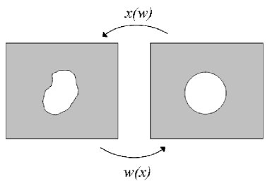
Figure 1: The conformal map $w(x)$ and its inverse $x(w)$.

The inverse conformal map takes the form of a semi-infinite Laurent polynomial,

$$x(w)=rw+\sum_{k>0}u_{k}w^{-k}\;,\;\;\;|w|>1\;.$$ (17)

The coefficient $r$ can be chosen to be real and positive. Our interest is the boundary of the domain. Therefore, we can take the limit where $w$ approaches the boundary of the unit disk: $w\rightarrow e^{i\phi}$. In this case we obtain the map, $x:S^{1}\rightarrow\partial{\cal D}$. In general, this map can be multi-valued, so we need to be careful in choosing the parameters of the conformal map to avoid this.

Once we have the inverse conformal map (17), we can convert any contour integral over $\partial{\cal D}$ to a holomorphic contour integral over $S^{1}$. For example, Eq. (8) becomes

$$V(z,\bar{z})=\oint_{S^{1}}\frac{dw}{2\pi i}x^{\prime}(w)\frac{1}{(x(w)-z)(\bar{x}(w^{-1})-\bar{z})}\;,$$ (18)

where the prime is the derivative with respect to $w$. The value of the integral will then be the sum of the residues of the simple poles in $w$ that are inside the unit circle.

Let us now note, that not all the parameters in the conformal map are independent. In our case, we need to impose the restriction on the area of the droplet. This is given by,

$$1 = \int_{\cal D}\frac{d^{2}z}{\pi}=\int_{\cal D}\frac{d^{2}z}{\pi}\bar{\partial}\bar{z}=\oint_{S^{1}}\frac{dw}{2\pi i}x^{\prime}(w)\bar{x}(w^{-1})\;.$$

It is very convenient to write the parameters of the inverse conformal map, in terms of the so-called “moments” of the domain ${\cal D}$. Assuming that we include the origin in the droplet, the moments are defined by ($k>0$),

$$t_{k}=\frac{1}{k}\oint_{\partial\cal D}\frac{dz}{2\pi i}\bar{z}z^{-k}=\frac{1}{k}\oint_{S^{1}}\frac{dw}{2\pi i}\frac{x^{\prime}(w)\bar{x}(w^{-1})}{x^{k}(w)}\;.$$ (20)

We will see that these moments translate directly to the parameters of the gauge theory operators.

III.2 Elliptical Droplet

For the elliptical droplet, we can use the simplest singular inverse map, $x(w)=rw+\frac{u}{w}$. Using the area normalization (III.1), we get, $1=r^{2}-|u|^{2}$. Without lost of generality we can take $u$ to be real . Using (20), one can see that the elliptical droplet has only $t_{2}\neq 0$. The inverse map can then be parameterized by,

$$x(w)=\frac{1}{\sqrt{1-\epsilon^{2}}}\left(w+\frac{\epsilon}{w}\right)\;,\;\;\;0\leq\epsilon<1\;,$$ (21)

where $\epsilon\equiv 2t_{2}$ is the eccentricity of the ellipse. The elliptical droplet is shown in figure 2.

Figure 2: Elliptical Droplet. We have chosen $t_{2}$ to be real.

The integrand in (18) has the form:

$$\frac{\sqrt{1-\epsilon^{2}}}{\epsilon}\frac{w^{2}-\epsilon}{(w-w_{1})(w-w_{2})(w-\bar{w}_{1}/\epsilon)(w-\bar{w}_{2}/\epsilon)}\;,$$ (22)

where the poles are given by,

$$w_{1,2}=\frac{1}{2}\sqrt{1-\epsilon^{2}}\left(z\pm\sqrt{z^{2}-\frac{4\epsilon}{1-\epsilon^{2}}}\right)\;.$$ (23)

Now we need to find out which poles are inside the unit circle. To do this, we note that in our coordinates, the origin $z=0$ will always be included inside the droplet. Moreover, we do not want to encounter any singularities in $V$ as we move away from the origin (unless we hit the boundary of the droplet).

For this, the number of poles inside the unit circle has to remain unchanged as we smoothly move away from the origin. Therefore, we can evaluate the poles at the origin to see whether they are inside or outside the unit circle. Doing this, we find that $|w_{1,2}|^{2}=\epsilon<1$. Moreover, $|w_{1,2}|^{2}/\epsilon^{2}=1/{\epsilon}>1$. Therefore, only $w_{1,2}$ will be inside the unit circle. Summing the residues for finite $z$ we get our final result,

$$V=\frac{z(1+\epsilon^{2})-2\epsilon\bar{z}}{1-\epsilon^{2}+\epsilon(z^{2}+\bar{z}^{2})-|z|^{2}(1+\epsilon^{2})}=\bar{\partial}\log K\;,$$ (24)

where,

$$K(z,\bar{z})=\frac{1}{1-\epsilon^{2}+\epsilon(z^{2}+\bar{z}^{2})-|z|^{2}(1+\epsilon^{2})}\;.$$ (25)

Note that $K=\infty$ gives the equation of the ellipse with eccentricity $\epsilon$ growth . Moreover, for $\epsilon=0$ we recover the usual result, $V=z/(1-|z|^{2})$ which was found in sam1 ; sam2 in the context of open strings on Giant Gravitons.

III.3 Hypotrochoid

The Hypotrochoid is shown in figure 3.

Figure 3: Hypotrochoid. We have chosen $t_{3}$ to be real.

This is another one-parameter family of droplets. It has been also studied in the context of normal random matrix theory growth ; sing . The only non-zero moment is $t_{3}$. The inverse of the conformal map is given by,

$$x(w)=rw+\frac{u}{w^{2}}\;.$$ (26)

The parameters are related by Eqs. (III.1) and (20),

$$1=r^{2}(1-2a^{2}r^{2})\;,\;\;\;u=3t_{3}r^{2}\equiv ar^{2}\;.$$ (27)

Again, one can take $u$ to be real without lost of generality.

If we vary $a$, we find that the boundary of the droplet develop singularities at $a>1/\sqrt{8}$. This kind of singular behavior has been studied from the point of view of random matrix theory sing . The String Theory interpretation is not clear, but it would be interesting to understand it. This is, however, outside of the scope of this paper. In any case, these singularities are of no concern since, in what follows, we will only expand near small $a$.

We can now calculate $V$ from (18) as before. One finds that the integrand contains the inverse of a sixth order polynomial in $w$. Only three roots are inside the circle. The resulting expression is quite complicated, so we will only show the first four orders in $a$:

$$V = \frac{z}{1-|z|^{2}}-\frac{\left(z^{4}+{{\bar{z}}}^{2}\,\left(3-2\,z\,{\bar{z}}\right)\right)\,a}{{\left(1-|z|^{2}\right)}^{2}}$$

$$+\frac{\left(2\,z+z^{7}+3\,{{\bar{z}}}^{5}-2\,z\,{{\bar{z}}}^{6}\right)\,a^{2}}{{\left(1-|z|^{2}\right)}^{3}}$$

$$-\frac{\left(z^{4}\,\left(3+z^{6}\right)+3\,{{\bar{z}}}^{2}+3\,{{\bar{z}}}^{8}-2\,z\,{{\bar{z}}}^{9}\right)\,a^{3}}{{\left(1-|z|^{2}\right)}^{4}}+{\cal O}(a^{4})\;.$$

In the section VI, we will see how a gauge theory calculation can reproduce this non-trivial result.

III.4 Laplacian Growth

In this section, we will briefly mention how to construct a one-to-one map from the interior of a simply-connected droplet, to the interior of the unit disk. We will find a “quantum” version of this map in the gauge theory.

Suppose that we normalize the area of the droplet according to,

$$\int_{\cal D}d^{2}z\rho=\int_{D_{R}}d^{2}z\rho\;,$$ (29)

where $D_{R}$ is circular disk of radius $R\leq 1$. Our new normalization condition is then,

$$R^{2}=\oint_{\partial\cal D}\frac{dz}{\pi}\bar{z}\;.$$ (30)

Now consider varying $R$, but keeping the moments $t_{k}$ defined in (20) fixed. This process is known as Laplacian Growth (or shrink, if we decrease $R$) matrixreview ; growth . That is, varying $R$ gives “concentric” droplets.

Using the inverse-conformal map (17), one can construct the the desired map from the interior of the unit disk ($D_{1}$), to the interior of the droplet:

$$L(y)\equiv x(R,w=e^{i\phi})\in{\cal D}\;,\;\;\;y\equiv Rw=Re^{i\phi}\in D_{1}\;.$$ (31)

We will call $L(y)$ the “Laplacian Map”.

Let us give some explicit examples. For the elliptical droplet, the map is constructed from the normalization equations (20) and (30): $R^{2}=r^{2}-|u|^{2}$, $u=\epsilon r$. We get,

$$L(y)=\frac{1}{\sqrt{1-\epsilon^{2}}}\left(y+\epsilon\bar{y}\right)\;.$$ (32)

For the Hypotrochoid, one needs to solve, $R^{2}=r^{2}(1-2a^{2}r^{2})$ and $u=ar^{2}$. We get,

$$L(y)=r\left(y+ar\bar{y}^{2}\right)\;,$$ (33)

where

$$r=\left(\frac{1-{\sqrt{1-8a^{2}|y|^{2}}}}{4a^{2}|y|^{2}}\right)^{1/2}\;.$$ (34)

Expanding to ${\cal O}(a^{3})$ we get,

$$L(y)\approx(1+a^{2}|y|^{2})y+a(1+2a^{2}|y|^{2})\bar{y}^{2}+{\cal O}(a^{4})\;.$$ (35)

IV Gauge Theory Despcription: General Results

In this section, we show how the reduced sigma model (16) arises directly from the one-loop dilatation operator of $\cal N$ = 4 SYM in the $SU(2)$ sector. We will do this by translating the problem to the language of Random Matrix Theory. Our procedure is very general, and works for any droplet configuration, including the case of multiple connected domains. Moreover, it is straightforward to extend beyond one loop. We will find that the dilatation operator for any droplet can be interpreted as a dynamical spin chain. By “dynamical”, we mean that the length of the chain is not conserved and spins can enter and leave the lattice.

IV.1 Review and Notation

The standard operator-state correspondence of ${\cal N}=4$ SYM allows us to define a basis for the Hilbert space of states in $\mathbb{R}\times S^{3}$ in terms of local operators in $\mathbb{R}^{1,3}$. The inner product in the Hilbert space is then mapped to correlation functions of local operators. The inner product is defined at zero coupling. If we work only in the scalar sector of the theory, we can normalize the local operators such that the propagator takes the form,

$${\langle}X_{i}^{j}(x)\bar{X}_{k}^{l}(0){\rangle}=\delta_{i}^{l}\delta_{k}^{j}\;,$$ (36)

where $X$ is any of the three complex scalars of SYM. This is the usual propagator for a gaussian random matrix model of a single complex matrix. Thus, we can just drop the space-time dependence of the operators, and compute all free-field theory correlation functions using the gaussian matrix model.

Increasing the coupling away from zero, produces logarithmic divergences in the OPEs. Extracting these divergences gives the action of the Dilatation operator. However, the combinatorics can still be encoded in a simple gaussian matrix model.

In the $SU(2)$ sector, the operators have the general form,

$$\psi\sim\hbox{ Tr}(YZYZZ\cdots)\hbox{ Tr}(ZYZZ\cdots)\cdots\;.$$ (37)

The dilatation operator acts on these operators as beisert ,

$$\hat{D}-\hat{J}\equiv\hat{H}=-\frac{g_{YM}^{2}}{8\pi^{2}}\hbox{ Tr}[Z,Y][\partial_{Z},\partial_{Y}]+\ldots$$ (38)

The dots indicate higher loop contributions, and we have subtracted the R-charge operator ($\hat{J}$). Moreover, the derivatives have the property that $(\partial_{Z})_{i}^{j}Z_{k}^{l}=\delta_{i}^{l}\delta_{k}^{j}$.

An orthonormal basis in this sector is composed of operators such that,

$${\langle}\psi_{n}|\psi_{m}{\rangle}={\langle}\psi_{n}^{*}(\bar{Y},\bar{Z})\psi_{m}(Y,Z){\rangle}=\delta_{nm}\;,$$ (39)

where, as usual,

$${\langle}{\cal O}{\rangle}=\frac{\int[d^{2}Yd^{2}Z]e^{-\hbox{ Tr}(|Z|^{2}+|Y|^{2})}{\cal O}}{\int[d^{2}Yd^{2}Z]e^{-\hbox{ Tr}(|Z|^{2}+|Y|^{2})}}.$$ (40)

Here, $[d^{2}Yd^{2}Y]$ is the standard $U(N)$ invariant measure defined by the metric, $ds^{2}=\hbox{ Tr}(dYd\bar{Y}+dZd\bar{Z})$. The matrix elements of the dilatation operator are defined in the usual way,

$$(\hat{H})_{nm}={\langle}\psi_{n}^{*}(\bar{Y},\bar{Z})\hat{H}\psi_{m}(Y,Z){\rangle}\;.$$ (41)

It is now convenient to rescale our fields as $(Y,Z)\rightarrow(Y,Z)/\sqrt{\hbar}$, where $\hbar=1/N$. In this way, correlation functions will be order one in the large $N$ limit ($\hbar\rightarrow 0$).

The 1/2 BPS sector is given by any holomorphic wavefunction on (say) $Z$. One obviously has, $\hat{H}\psi(Z)=0$. In this special case one can integrate out the off-diagonal components of $Z$. This is done by expanding $Z=U^{\dagger}(Z_{\text{diag.}}+R)U$, where $Z_{\text{diag.}}$ is a diagonal matrix, $R$ is an upper-triangular matrix and $U\in U(N)$. It turns out that the measure of the matrix model transforms as matrixreview ,

$$[d^{2}Z]e^{-\hbox{ Tr}(|Z|^{2})/\hbar} = \prod_{i<j}\left(d^{2}R_{i}^{j}e^{-|R_{i}^{j}|^{2}/\hbar}\right)$$

$$\times\prod_{k}d^{2}z_{k}e^{-|z_{k}|^{2}/\hbar}\prod_{l<m}|z_{l}-z_{m}|^{2}\;.$$

Since $\hbox{ Tr}((Z_{\text{diag.}}+R)^{n})=\hbox{ Tr}(Z^{n})$, the matrix $R$ drops from all holomorphic states. All correlation functions are then expressed in terms of the eigenvalues $Z_{\text{diag.}}$.

We can now consider a “heavy” 1/2 BPS state such as,

$${\psi}=e^{\hbox{ Tr}\;\Omega(Z)/\hbar}\;.$$ (43)

The normalization of such a state is given by the partition function,

$${\langle}{\psi}|{\psi}{\rangle}\propto\prod_{i=1}^{N}\int d^{2}z_{i}e^{\sum_{j}W(z_{j},\bar{z}_{j})/\hbar+\sum_{i<j}\log|z_{i}-z_{j}|^{2}}\;,$$ (44)

where

$$W(z,\bar{z})=-|z|^{2}+\Omega(z)+\overline{\Omega(z)}\;.$$ (45)

It is well known that in the “classical” limit $\hbar\rightarrow 0$, the eigenvalues condense into constant density droplets matrixreview ; growth in the complex plane. This is the usual 2D Coulomb gas problem. In fact, the density of the droplets is $\rho=1/(\hbar\pi)$.

This matches the String Theory classification of the 1/2 BPS geometries. However, reconstructing the form of the droplets given the potential $\Omega(z)$, is a non-trivial inverse problem that has been the subject of numerous papers. We will not need to go into these details here, since we will find a new way of doing this.

Nevertheless, for the case of a single droplet, the problem simplifies dramatically. One can show matrixreview that the moments introduced in (20) are related to the potential as,

$$\Omega(z)=\sum_{k>0}t_{k}z^{k}\;.$$ (46)

This allow us to reconstruct the operator dual to any single-droplet space-time.

One can also consider potentials that generate multiple droplets. These potentials have been studied in multdomain . Furthermore, to introduce “holes” in the droplets one must consider potentials such as $\Omega(z)\sim\sum_{k}a_{k}\log(z-b_{k})$. In particular, for a single hole in the center of the circular droplet, one has $\Omega(z)\sim\log z$. This last potential was studied in logdrop . As we will see, our formalism would need to be slightly modified for this special case, since $\Omega^{\prime}(z)$ is singular at $z=0$. However, it should still be applicable all other potentials that admit a power law expansion around $z=0$.

IV.2 Probe String Hilbert Space

In this section, we will prove some general results that are applicable for any potential $\Omega(z)$ whose first derivative $\Omega^{\prime}(z)$ admits a power-law expansion around $z=0$. Moreover, we will always work in the large $N$ limit.

Let us consider a “probe string” in a 1/2 BPS geometry. This can be mapped to a periodic lattice,

$$|n_{1},\ldots,n_{L}{\rangle}=\hbox{ Tr}(Y\psi_{n_{1}}(Z)Y\cdots Y\psi_{n_{L}}(Z))e^{\hbox{ Tr}\;\Omega(Z)/\hbar}\;,$$ (47)

with some unknown functions $\psi_{n}(Z)$. In the large $N$ limit, the normalization of this state is simply given by,

$${\langle}n_{1},\ldots,n_{L}|n_{1}^{\prime},\ldots,n_{L}^{\prime}{\rangle}\approx\prod_{l=1}^{L}{\langle}\hbar\hbox{ Tr}(\overline{\psi_{n_{l}}(Z)}\psi_{n_{l}^{\prime}}(Z)){\rangle}\;,$$ (48)

where we are considering the generic case where not all $n_{i}$ are equal to $n_{i}^{\prime}$. At this point, it is convenient to absorb the factors of $\hbar$ in the normalization of $\psi_{n}$. The functions $\psi_{n}(Z)$ must admit a power law expansion in $Z$. Moreover, we define $|0{\rangle}\cong\psi_{0}(Z)\equiv\sqrt{\hbar}\mathbf{1}$. The alert reader might wonder if $\psi_{n}$ could also include multiple traces. For example $(\psi)_{i}^{j}\sim\hbox{ Tr}(Z^{2})Z_{i}^{j}+\cdots$. However, one quickly realizes that, since correlation functions factorize in the large $N$ limit, one can treat these additional traces as numbers. That is, just replace (for example) $\hbox{ Tr}(Z^{2})\rightarrow{\langle}\hbox{ Tr}(Z^{2}){\rangle}$.

The correlation functions in (48) are computed including the potential $\Omega$,

$${\langle}{\cal O}{\rangle} = \frac{\int[d^{2}Z]e^{\hbox{ Tr}W/\hbar}{\cal O}}{\int[d^{2}Z]e^{\hbox{ Tr}W/\hbar}}\;,$$ (49)

where $W$ is given by (45). Thus, our first task is to find an orthonormal basis such that,

$${\langle}\hbox{ Tr}(\overline{\psi_{n}(Z)}\psi_{m}(Z)){\rangle}=\delta_{nm}\;.$$ (50)

For a general potential $\Omega$, this is a highly non-trivial problem, because the off-diagonal elements of $Z$ cannot be decoupled. To the best of the author’s knowledge, this problem has not been solved in the Random Matrix Theory literature. Here we will find a purely algebraic solution to it (in the large $N$ limit). In fact, the procedure is very similar to the construction of the orthogonal polynomials for the Normal Matrix Model growth .

Lets start by assuming the existence of the orthonormal basis (50). One can now define the operator

$$(\hat{L}^{\dagger})_{nm}={\langle}\hbox{ Tr}[\overline{\psi_{n}(Z)}Z\psi_{m}(Z)]{\rangle}\;,$$ (51)

and its conjugate,

$$(\hat{L})_{nm} = {\langle}\hbox{ Tr}[\bar{Z}\overline{\psi_{n}(Z)}\psi_{m}(Z)]{\rangle}$$ (52)

$$= {\langle}\hbox{ Tr}[\overline{\psi_{n}(Z)}(\hbar\partial_{Z}+\Omega^{\prime}(Z))\psi_{m}(Z)]{\rangle}\;,$$

where the second equality follows by integrating by parts in the matrix model. Then, one can prove the following theorem:

Theorem: The operators $\hat{L}^{\dagger}$ and $\hat{L}$ obey the algebra,

$$[\hat{L},\hat{L}^{\dagger}]=\hat{P}_{0}\;,$$ (53)

$$\hat{L}=\Omega^{\prime}(\hat{L}^{\dagger})+(\hat{L}^{\dagger})^{-1}+\sum_{k>1}v^{(k)}(\hat{L}^{\dagger})^{-k}\;,$$ (54)

where $\hat{P}_{0}$ is the projection to $|0{\rangle}$, and $(\hat{L}^{\dagger})^{-1}$ is defined by left multiplication on $\hat{L}$. Moreover, $v^{(k)}$ are constants given by,

$$v^{(k)}=\hbar\int d^{2}z\rho(z,\bar{z})z^{k-1}\;\;\;\;\;(k>1)\;,$$ (55)

where $\rho$ is the eigenvalue distribution of the matrix model.

Proof: Lets start by proving (53). For this, we first need to look at a monomial of $\psi_{n}$. We have,

$$[\hat{L},\hat{L}^{\dagger}]Z^{m} = \hbar(\partial_{Z}Z-Z\partial_{Z})Z^{m}$$ (56)

$$= Z^{m}+\sum_{k\geq 1}\hbar\hbox{ Tr}(Z^{k})Z^{m-k}$$

$$-Z\left(Z^{m-1}+\sum_{k\geq 1}\hbar\hbox{ Tr}(Z^{k})Z^{m-k-1}\right)$$

$$= \delta_{m,0}+\hbar\sum_{k\geq 1}\delta_{m,k}\hbox{ Tr}(Z^{k})\;.$$

In the large $N$ limit, we have

$${\langle}\hbox{ Tr}(\bar{\psi}_{n}[\hat{L},\hat{L}^{\dagger}]\sqrt{\hbar}Z^{m}){\rangle} \approx {\langle}\sqrt{\hbar}\hbox{ Tr}(\bar{\psi}_{n}){\rangle}{\langle}\delta_{m,0}$$ (57)

$$+\hbar\sum_{k\geq 1}\delta_{m,k}\hbox{ Tr}(Z^{k}){\rangle}$$

$$= \delta_{n,0}c_{m}\;,$$

for some constant $c_{m}$.

Note that in the Hilbert Space,

$${\langle}0|M_{m}{\rangle}=\hbar{\langle}\hbox{ Tr}(\mathbf{1}Z^{m}){\rangle}=c_{m}\;.$$ (58)

Here $|M_{m}{\rangle}=\sqrt{\hbar}Z^{m}$ is the state corresponding to a monomial, and $|0{\rangle}=\sqrt{\hbar}\mathbf{1}$. Note that we are normalizing states so that their inner product is of order one in the large $N$ limit.

Thus, we can write (57) as,

$${\langle}\psi|[\hat{L},\hat{L}^{\dagger}]|M_{m}{\rangle}={\langle}\psi|0{\rangle}{\langle}0|M_{m}{\rangle}={\langle}\psi_{n}|\hat{P}_{0}|M_{n}{\rangle}\;.$$ (59)

Since every state $|\psi_{n}{\rangle}$ is a linear superposition of monomials $|M_{n}{\rangle}$, Eq. (53) follows from (59).

Lets us now prove the second identity (54). This one follows directly form (52). The last two terms in (54) come from the matrix derivative in (52). For a monomial state, we get,

$${\langle}\hbox{ Tr}(\bar{\psi}_{n}\hbar\partial_{Z}\sqrt{\hbar}Z^{m}){\rangle} = \sum_{k>0}{\langle}\hbox{ Tr}(\bar{\psi}_{n}\sqrt{\hbar}Z^{m-k})\hbar\hbox{ Tr}(Z^{k-1}){\rangle}$$ (60)

$$\approx \sum_{k>0}{\langle}\hbox{ Tr}(\bar{\psi}_{n}\sqrt{\hbar}Z^{m-k}){\rangle}{\langle}\hbar\hbox{ Tr}(Z^{k-1}){\rangle}$$

$$\equiv \sum_{k>0}{\langle}\psi_{n}|(\hat{L}^{\dagger})^{-k}|M_{m}{\rangle}v^{(k)}\;,$$

where the last line defines the action of the inverse of $\hat{L}^{\dagger}$ and the constants $v^{(k)}$. The proof of (54) is completed by taking a superposition of monomials.

Since the coefficients $v^{(k)}$ are holomorphic correlation functions, they can be computed by an integration over the eigenvalue distribution as given in (55). For a single droplet distribution, we can write (55) as,

$$v^{(k)}=\oint_{\partial\cal D}\frac{dz}{2\pi i}\bar{z}z^{k-1}\;.$$ (61)

This completes the proof of the theorem. $\square$

In practice, one would like to find a particular representation of the algebra (53) and (54). In this case, we assume that the wavefunction $\psi_{n}(Z)$ is a polynomials of degree $n$. For the gaussian ensemble ($\Omega=0$) we have $\psi_{n}\sim Z^{n}$. Clearly, in the general case we will have

$$Z\psi_{n}(Z)=r_{n}\psi_{n+1}(Z)+\sum_{k\geq 0}u_{n}^{(k)}\psi_{n-k}(Z)\;.$$ (62)

Our goal will be to calculate the coefficients $r_{n},u_{n}^{(k)}$. Once this is done, the orthogonal polynomials can be calculated by iterating (62). Moreover, note that we can always define $u_{n}^{(k)}$ so that it gives zero for $k>n$.

We can now translate (62) to the Hilbert Space using (51) and (52). Namely,

$$\hat{L}^{\dagger} = \hat{a}^{\dagger}r_{n}+\sum_{k\geq 0}\hat{a}^{k}u_{n}^{(k)}\;,$$ (63)

$$\hat{L} = r_{n}\hat{a}+\sum_{k\geq 0}\bar{u}_{n}^{(k)}(\hat{a}^{\dagger})^{k}\;,$$ (64)

where

$$\hat{a}^{\dagger}|n{\rangle}=|n+1{\rangle}\;,\;\;\hat{a}|n{\rangle}=(1-\delta_{n,0})|n-1{\rangle}\;,$$ (65)

and now $r_{n},u_{n}^{(k)}$ are regarded as diagonal operators. Note that $\hat{a},\hat{a}^{\dagger}$ are the Cuntz oscillators used in sam1 ; sam2 . Moreover, one can always take $r_{n}$ to be real without lost of generality.

The inverse operator $(\hat{L}^{\dagger})^{-1}$ is defined by left multiplication on $\hat{L}$: $(\hat{L}^{\dagger})^{-1}\hat{L}^{\dagger}=1$. Explicitly,

$$(\hat{L}^{\dagger})^{-1} = [(r_{n-1}+\sum_{k\geq 0}\hat{a}^{k+1}u_{n}^{(k)})\hat{a}^{\dagger}]^{-1}$$ (66)

$$= \hat{a}\frac{1}{r_{n-1}+\sum_{k\geq 0}\hat{a}^{k+1}u_{n}^{(k)}}\;,$$

where the last expression is defined by its power expansion in $\hat{a}$.

The coefficients $r_{n}$ and $u_{n}^{(k)}$ in (63) and (64), are completely determined by the algebra (53) and (54). In particular, after some work, one can show that the diagonal part of (53) reads,

$$1=r_{n}^{2}-\sum_{k\geq 1}\sum_{p=0}^{n}|u_{n+k}^{(k+p)}|^{2}\;.$$ (67)

Summary: This section has been quite technical, so let us summarize the main results. The Hilbert space for a probe string in a generic 1/2 BPS geometry can be mapped to a periodic lattice as in (47). This basis is endowed with the algebra (53) and (54). One then assumes that the wavefunctions $\psi_{n}$ are polynomials. Their explicit form is defined by the recursion relation (62). The coefficients of the recursion relation are completely determined by the algebra (53) and (54), by using the representation (63) and (64).

IV.3 Hamiltonian

In this section, we will find the action of the Hamiltonian (38) in the probe string basis studied in the previous section. We will only work at one-loop. First, let us study the action on a particular $Y$ on the lattice,

$$\hat{H}|\cdots,n_{l},n_{l+1},\cdots{\rangle}=-\frac{g_{YM}^{2}N}{8\pi^{2}}\hbox{ Tr}[Z,Y][\hbar\partial_{Z},\partial_{Y}]$$

$$\times\hbox{ Tr}(\cdots\psi_{n_{l}}Y\psi_{n_{l+1}}\cdots)e^{\hbox{ Tr}\;\Omega(Z)/\hbar}$$

$$=-\frac{g_{YM}^{2}N}{8\pi^{2}}\left[\hbox{ Tr}(\cdots\psi_{n_{l}}[Z,Y]\hbar\overleftrightarrow{\partial_{Z}}\psi_{n_{l+1}}\cdots)\right.$$

$$\left.-\hbox{ Tr}(\cdots\psi_{n_{l}}\hbar\overleftrightarrow{\partial_{Z}}[Z,Y]\psi_{n_{l+1}}\cdots)\right]$$

$$\times e^{\hbox{ Tr}\;\Omega(Z)/\hbar}\;.$$ (68)

The double arrow means that the derivative acts on both sides but always excluding the $Z$ in the commutator. Note that the derivative will also act on the potential $\Omega(Z)$.

In the planar limit, one can show that multiple traces in $Y$ are still suppressed. Therefore, one must not allow the derivative to act beyond its own site. Then, it is easy to show that the action of the Hamiltonian has a remarkably simple form in terms of the operators (63) and (64):

$$\hat{H}=\lambda\sum_{l=1}^{L}(\hat{L}^{\dagger}_{l}-\hat{L}^{\dagger}_{l+1})(\hat{L}_{l}-\hat{L}_{l+1})\;,$$ (69)

where periodic boundary conditions are understood.

The form of the Hamiltonian (69), is very similar to the bosonized version of the ferromagnetic Heisenberg spin chain introduced in sam1 ; sam2 . In the general case, however, one has a complicated canonical structure given by (53) and (54).

To get the usual $XXX_{1/2}$ spin chain, one takes the simplest case of $\Omega=0$. This choice gives the disk distribution of eigenvalues. Using (61) one can easily prove $v^{(k)}=0$. Thus, the algebra (53) and (54) reduces to,

$$[\hat{L},\hat{L}^{\dagger}]=\hat{P}_{0}\;,\;\;\;\;\hat{L}\hat{L}^{\dagger}=1\;.$$ (70)

In other words:

$$\left.\hat{H}\right|_{\Omega=0}=\lambda\sum_{l=1}^{L}(\hat{a}^{\dagger}_{l}-\hat{a}^{\dagger}_{l+1})(\hat{a}_{l}-\hat{a}_{l+1})\;.$$ (71)

To translate this to the spin chain language, one makes the following identification sam1 ; sam2 ,

$$|n_{1},n_{2},\ldots,n_{L}{\rangle}=|\uparrow\underbrace{\downarrow\downarrow\cdots\downarrow}_{n_{1}}\uparrow\underbrace{\downarrow\downarrow\cdots\downarrow}_{n_{2}}\uparrow\cdots\uparrow\underbrace{\downarrow\downarrow\cdots\downarrow}_{n_{L}}{\rangle}\;.$$ (72)

In the spin chain basis, the Hamiltonian (71) can be written as

$$\left.\hat{H}\right|_{\Omega=0}=\lambda\sum_{l=1}^{J}\left(1-4\vec{S}_{l}\cdot\vec{S}_{l+1}\right)\;,$$ (73)

where $J=L+\sum_{l=1}^{L}n_{l}$. This is indeed the spin chain that was originally discovered in the context of the AdS/CFT correspondece in zarembo .

If we now consider the general case with $\Omega\neq 0$, one can easily see from (63), (64) and (69), that the number of “spin downs” in (72) will not be conserved. In other words, the length of the spin chain is not preserved. In this case, the best interpretation for the Hamiltonian (69), is as a bosonic lattice with $n_{l}$ bosons at each site. Moreover, the bosons can leave or enter the lattice at any site. This kind of dynamical lattice was first found in sam1 ; sam2 in the study of Giant Gravitons. Dynamical lattices have also been studied (in a different context) in dynamicspin ; condmatter .

IV.4 Coherent States and Space-Time Metric

If we want to gain insight into the classical limit of the Hamiltonian (69), one must construct coherent states of the operator $\hat{L}$. Making the general ansatz for the coherent states:

$$|z{\rangle}=\sum_{n=0}^{\infty}f_{n}(z)|n{\rangle}\;,$$ (74)

it is easy to show that one needs,

$$zf_{n}(z)=r_{n}f_{n+1}(z)+\sum_{k\geq 0}\bar{u}_{n}^{(k)}f_{n-k}(z)\;.$$ (75)

So we see that $f_{n}$ are really the complex conjugate of the wavefunctions (62):

$$f_{n}(z)=\psi_{n}^{*}(z)\;.$$ (76)

Moreover, the range of the coordinate $z$ will be given by the normalization condition,

$$0\leq{\langle}z|z{\rangle}<\infty\;.$$ (77)

This condition will give us the shape of the droplet.

Now, we have not proved that these coherent states are (over)complete. This is, in general, very difficult. We remind the reader that, even for the simple case of the gaussian ensemble with $f_{n}=z^{n}$, the completeness relation requires to introduce a very special measure in terms of the so-called “Jackson Integral” sam1 ; sam2 . This turns out to be irrelevant in our case, since we will only use the coherent states in the classical limit, where the measure of the path integral can be ignored. So from now on, we just assume that a measure exist, such that $1=\int d\mu(z,\bar{z})|z{\rangle}{\langle}z|$.

In this case, one can always write the classical action for a general coherent state $|CS{\rangle}$ as coh ,

$$S=\int d\tau\left(i{\langle}CS|\partial_{\tau}|CS{\rangle}-{\langle}CS|\hat{H}|CS{\rangle}\right)\;.$$ (78)

In our case this reduces to,

$$S = \int d\tau\sum_{l=1}^{L}\left(i{\langle}z_{l}|\partial_{\tau}|z_{l}{\rangle}-\lambda|z_{l}-z_{l+1}|^{2}\right)$$ (79)

$$\rightarrow -L\int d\tau\int_{0}^{1}d\sigma\left(\frac{i}{2}V\dot{\bar{z}}-\frac{i}{2}\bar{V}\dot{z}+\frac{\lambda}{L^{2}}|z^{\prime}|^{2}\right)\;,$$

where

$$V=\bar{\partial}\log\left(\sum_{n=0}^{\infty}|\psi_{n}(\bar{z})|^{2}\right)\;.$$ (80)

Therefore, we find that in the thermodynamic limit $L\rightarrow\infty$, the coherent state action of our quantum lattice has the same form as the String Theory result (16). The extra constant in (16) can be obtained if we add the R-charge operator $\hat{J}_{Y}=\hbox{ Tr}(Y\partial_{Y})$.

One can readily identify the function $V$ defined in (80) with the one-form (8). Moreover, from (9) we can also reconstruct the remaining function in the metric,

$$h^{4}=\partial\bar{\partial}\log\left(\sum_{n=0}^{\infty}|\psi_{n}(\bar{z})|^{2}\right)\;.$$ (81)

The reader can easily verify that for the circular droplet, with $\psi_{n}=z^{n}$, both (80) and (81) reduce to the familiar results,

$$V=\frac{z}{1-|z|^{2}}\;,\;\;\;h^{4}=\frac{1}{(1-|z|^{2})^{2}}\;.$$ (82)

In practice, in order to perform the sum over the orthogonal polynomials, one needs to find their generating function:

$$G(z,x)=\sum_{n=0}^{\infty}f_{n}(z)x^{n}\;.$$ (83)

For a general droplet, this is a difficult object to construct. However, we will see that one can set up a systematic expansion around the circular droplet.

V Example 1: Elliptical Droplet

This is the simplest droplet next to the circular one. It is generated by the simple potential $\Omega(z)=t_{2}z^{2}$. From (54) it is easy to see that $\hat{L}^{\dagger}$ will truncate at ${\cal O}(\hat{a})$:

$$\hat{L}^{\dagger}=\hat{a}^{\dagger}r_{n}+u^{(0)}+\hat{a}u^{(1)}_{n}\;.$$ (84)

Collecting terms of ${\cal O}(\hat{a}^{\dagger})$ and ${\cal O}(1)$ in (54) one finds that,

$$\frac{\bar{u}^{(0)}_{n}}{u_{n}^{(0)}}=\epsilon\;,\;\;\;\frac{\bar{u}_{n}^{(1)}}{r_{n+1}}=\epsilon\;,$$ (85)

where $\epsilon=2t_{2}$. Since we want to be able to consider the case $\epsilon<1$, it follows that $u_{n}^{(0)}=0$. Moreover, from (67) it follows that,

$$1=r_{n}^{2}-|u_{n+1}|^{2}\;.$$ (86)

Thus, we find

$$r_{n}=\frac{1}{\sqrt{1-\epsilon^{2}}}\;,\;\;\;u_{n}=\frac{\epsilon}{\sqrt{1-\epsilon^{2}}}\;,$$ (87)

where we have chosen $\epsilon$ real without lost of generality.

One can explicitly check that the other non-diagonal terms in (54) are indeed satisfied. For example, at ${\cal O}(\hat{a})$ one gets the equation,

$${\hat{a}}(1-r_{n}^{2}+\epsilon\;u_{n}r_{n})=0\;.$$ (88)

which is easily seen to be satisfied if we use (87).

We can now find the generating function of the polynomials by using their recursion relation:

$$zG(z,x)=\sum_{n=0}^{\infty}\left(\frac{1}{\sqrt{1-\epsilon^{2}}}f_{n+1}+\frac{\epsilon}{\sqrt{1-\epsilon^{2}}}f_{n-1}\right)x^{n}\;,$$ (89)

from where we find,

$$G(z,x)=\frac{1}{\epsilon x^{2}-\sqrt{1-\epsilon^{2}}xz+1}\;.$$ (90)

This is, in fact, the generating function of the Chebyshev Polynomials of the Second Kind.

The sum over the orthogonal polynomials can be calculated, in general, from

$$\sum_{n=0}^{\infty}|f_{n}(z)|^{2}=\oint_{S^{1}}\frac{dx}{2\pi i}\frac{1}{x}G(z,x)\bar{G}(\bar{z},1/x)\;.$$ (91)

We can calculate this integral explicitly using the Residue Theorem. Just like in the String Theory calculations, one can find out which pole is inside the unit circle by slowly moving away from the point $z=0$. Alternatively, one can require that the solution should be continuously connected with the case $\epsilon=0$. In any case, one finds that the only poles inside the unit circle are the roots of the quadratic equation,

$$\epsilon-\sqrt{1-\epsilon^{2}}\bar{z}x+x^{2}=0\;.$$ (92)

The sum of the residues gives,

$$\sum_{n=0}^{\infty}|f_{n}(z)|^{2}=\frac{1}{1-\epsilon^{2}+\epsilon(z^{2}+\bar{z}^{2})-|z|^{2}(1+\epsilon^{2})}\;.$$ (93)

This is exactly what we found in the String Theory calculation! From this “Kahler Potential” we can reconstruct the whole metric using (80) and (81). We clearly see that the shape of the droplet coincides with the range of $z$ that gives normalizable coherent states (c.f. (77)).

We want to point out that the elliptical droplet is rather special. One can, in fact, find the explicit form of the orthogonal polynomials by a direct matrix model calculation. Using a simple shift in the integration variables in the matrix model partition function, one can show,

$$e^{2\hbox{ Tr}(|X|^{2})/\epsilon}={\langle}e^{\hbox{ Tr}(-X^{2}+\alpha ZX)}e^{\hbox{ Tr}(-\bar{X}^{2}+\alpha\bar{Z}\bar{X})}{\rangle}\;,$$ (94)

where $\alpha=\sqrt{2(1-\epsilon^{2})/\epsilon}$.

The orthogonal matrix polynomials are given by,

$$\psi_{n}(Z)=\sqrt{\frac{\epsilon}{2N^{n+1}}}\,(\partial_{X})^{n}\left.e^{\hbox{ Tr}(-X^{2}+\alpha ZX)}\right|_{X=0}\;.$$ (95)

In the large $N$ limit, the derivatives $\partial_{X}$ must act in such a way as to avoid the creation of multiple traces in $\partial_{X}$. Moreover, we need to remember that any multiple traces in $Z$ must be replaced by their expectation value. Then, it is easy to show that these are the same polynomials as the ones found above.

Let us close this section with an interesting observation regarding the operator $\hat{L}$. Let us identify the operators $\hat{a}$ and $\hat{a}^{\dagger}$ as coordinates on a unit disk:

$$\hat{a}\sim y\;,\;\;\;\hat{a}^{\dagger}\sim\bar{y}\;,\;\;\;y\in D_{1}\;.$$ (96)

This identification actually follows from the coherent states of the operator $\hat{a}$ which are normalized only inside the unit disk sam1 ; sam2 .

With this identification, the operator $\hat{L}$ can be seen to give the classical map (32) from $D_{1}$ to the interior of the elliptical droplet. We will find that, in general, $\hat{L}$ gives a “quantum” version of this map (for a single droplet).

VI Example 2: Hypotrochoid

This droplet is another example of a one-parameter family of potentials given by $\Omega(z)=t_{3}z^{3}$. From Eq. (54), one can see that the operator $\hat{L}$ must truncate at ${\cal O}((\hat{a}^{\dagger})^{2})$. Thus, we are left with the ansatz,

$$\hat{L}=r_{n}\hat{a}+\bar{u}^{(0)}_{n}+\bar{u}^{(1)}_{n}\hat{a}^{\dagger}+\bar{u}_{n}^{(2)}(\hat{a}^{\dagger})^{2}\;.$$ (97)

Solving the recursion relations with this general ansatz is very cumbersome. However, one can make the simplifying assumption that $u_{n}^{(0)}=u_{n}^{(1)}=0$. The motivation for this, is the similarity between the operator $\hat{L}$ and the conformal map (26) (for a single droplet). This same kind of assumptions are used in the context of the classical orthogonal polynomials growth . We will latter see that this is a self-consistent assumption.

With this simplification, the ${\cal O}((\hat{a}^{\dagger})^{2})$ term from (54) gives the relation,

$$\bar{u}_{n}^{(2)}=ar_{n-1}r_{n-2}\;,$$ (98)

where we have defined $a\equiv 3t_{3}$ which we take to be real without lost of generality. Finally, Eq. (67) gives,

$$1=r_{n}^{2}-|u_{n+1}^{(2)}|^{2}(1-\delta_{n,0})-|u_{n+2}^{(2)}|^{2}\;.$$ (99)

Therefore, we get a closed equation for $r_{n}$:

$$1=r_{n}^{2}[1-a^{2}(r_{n-1}^{2}(1-\delta_{n,0})+r_{n+1}^{2})]\;.$$ (100)

One can solve this order by order in $a$. We have,

$$r_{n}^{2}\approx 1+a^{2}(2-\delta_{n,0})+{\cal O}(a^{4})\;.$$ (101)

Using this result in (98) we obtain,

$$u_{n}^{(2)}\approx a+a^{3}\left(2-\frac{1}{2}\delta_{n-2,0}\right)+{\cal O}(a^{5})\;.$$ (102)

Note that we have discarded the term with $\delta_{(n-1),0}$ since we always have $n\geq 2$ for this operator.

These results allow us to reconstruct the recurrence relation for the coherent states. Namely,

$$zf_{n}(z) = \left[\left(1+\frac{1}{2}a^{2}\right)+\frac{1}{2}a^{2}\left(1-\delta_{n,0}\right)\right]f_{n+1}(z)$$ (103)

$$+\left[a\left(1+\frac{3}{2}a^{2}\right)+\frac{1}{2}a^{3}\left(1-\delta_{n,2}\right)\right]f_{n-2}(z)$$

$$+{\cal O}(a^{4})\;.$$

This recurrence relation allow us to solve for the generating function to ${\cal O}(a^{3})$ accuracy. We have,

$$zG(z,x) = \frac{1}{x}\left(1+\frac{1}{2}a^{2}\right)\left(G(z,x)-1\right)$$ (104)

$$+\frac{1}{2x}a^{2}\left(G(z,x)-1-f_{1}(z)x\right)$$

$$+a\left(1+\frac{3}{2}a^{2}\right)x^{2}G(z,x)+\frac{1}{2}a^{3}x^{2}\left(G(z,x)-1\right)$$

$$+{\cal O}(a^{4})\;.$$

The polynomial $f_{1}(z)$ can be constructed explicitly from the recursion formula (103),

$$f_{1}(z)=\frac{z}{1+\frac{1}{2}a^{2}}\;.$$ (105)

Note that this formula should only be understood as an approximation which is good to order $a^{3}$.

The generating function can now be explicitly written as,

$$G(z,x)\approx\frac{\left(2+a^{2}\right)\,\left(2+a^{2}\,\left(2+a\,x^{3}\right)\right)+2\,a^{2}\,x\,z}{2\,\left(2+a^{2}\right)\,\left(1+a\,\left(a+x^{3}+2\,a^{2}\,x^{3}\right)-x\,z\right)}\;.$$ (106)

In this last result, we have chosen not to expand in powers of $a$, since the singularity of $G$ is very important for the next calculation. However, one must keep in mind that the final result is only valid up to corrections of order $a^{4}$.

To calculate the sum of the orthogonal polynomials, we use (91). Following a similar procedure as with the elliptical droplet, one finds that the integrand has simple poles inside the unit circle for $x=0$, and at the roots of,

$$a+2a^{3}-\bar{z}x^{2}+(1+a^{3})x^{3}=0\;.$$ (107)

The final sum over the residues is quite complicated, but the one form $V$ (c.f. Eq. (80)) simplifies a bit. The answer turns out to be exactly the one found in the String Theory calculation, Eq. (III.3)!

Let us now return to the interpretation of $\hat{L}$ as the Laplacian map. Using our results for $r_{n}$ and $u_{n}^{(2)}$ one can write $\hat{L}$ as,

$$\hat{L} \approx \left(1+\frac{1}{2}a^{2}\hat{a}^{\dagger}\hat{a}\right)\hat{a}+\hat{a}\left(\frac{1}{2}a^{2}\hat{a}^{\dagger}\hat{a}\right)$$ (108)

$$+a\left(1+\frac{3}{2}a^{2}\hat{a}^{\dagger}\hat{a}\right)(\hat{a}^{\dagger})^{2}$$

$$+\frac{1}{2}a^{3}(\hat{a}^{\dagger})^{2}\hat{a}^{\dagger}\hat{a}+{\cal O}(a^{4})\;.$$

If we interpret $\hat{a}\sim y$ and $\hat{a}^{\dagger}\sim\bar{y}$ as coordinates on $D_{1}$, and we ignore their ordering, one obtains precisely the Laplacian map (33). Note, however, that some of the terms in (108) are trivial (e.g. $\hat{a}\hat{a}^{\dagger}\hat{a}=\hat{a}$). Nevertheless, they are important for the interpretation as a Laplacian Map.

To finish this section, let us check that our initial assumption, $u_{n}^{(0)}=0=u_{n}^{(1)}$, is consistent. For this, we can just check explicitly the orthonormality of some of the polynomials $\psi_{n}(Z)$. Let us consider some examples.

The first few polynomials that follow from the generating function (106) are (remember that $f_{n}(z)=\psi_{n}^{*}(z)$, and we are taking $a$ to be real),

$$\psi_{0}(Z) = 1\;,$$ (109)

$$\psi_{1}(Z) = Z\left(1-\frac{1}{2}a^{2}\right)+{\cal O}(a^{4})\;,$$ (110)

$$\psi_{2}(Z) = Z^{2}\left(1-\frac{3}{2}a^{2}\right)+{\cal O}(a^{4})\;,$$ (111)

$$\psi_{3}(Z) = Z^{3}\left(1-\frac{5}{2}a^{2}\right)-a\left(1+\frac{1}{2}a^{2}\right)+{\cal O}(a^{4})\;,$$ (112)

$$\psi_{4}(Z) = Z^{4}\left(1-\frac{7}{2}a^{2}\right)-2aZ+{\cal O}(a^{4})\;.$$ (113)

The simplest orthogonality condition to check is ${\langle}0|n{\rangle}=0$, which in matrix form reads,

$${\langle}0|n{\rangle} = {\langle}\hbar\hbox{ Tr}(\overline{\psi_{0}(Z)}\psi_{n}(Z){\rangle}$$ (114)

$$= \int_{\cal D}\frac{d^{2}z}{\pi}\psi_{n}(z)$$

$$= \oint_{\partial\cal D}\frac{dz}{2\pi i}\bar{z}\psi_{n}(z)$$

$$= \oint_{S^{1}}\frac{dw}{2\pi i}x^{\prime}(w)\bar{x}(w^{-1})\psi_{n}(x(w))\;,$$

where $x(w)$ is given in (26). One can check explicitly that this expression is zero since there are no simple poles inside $S^{1}$.

Now, let us consider some non-trivial cases, where the off-diagonal elements of $Z$ do not drop out. As an example, we can calculate the normalization of $\psi_{1}(Z)$. Using the measure change (IV.1), we get

$${\langle}1|1{\rangle} = (1-a^{2}+{\cal O}(a^{4})){\langle}\hbar\hbox{ Tr}(|Z|^{2}){\rangle}$$ (115)

$$= (1-a^{2}+{\cal O}(a^{4}))\left(\hbar{\langle}\hbox{ Tr}(|Z_{\text{diag.}}|^{2}){\rangle}+\hbar{\langle}\hbox{ Tr}(\bar{R}R){\rangle}\right)$$

$$\approx (1-a^{2}+{\cal O}(a^{4}))\left(\frac{1}{2}\oint_{\partial\cal D}\frac{d^{2}z}{2\pi i}\bar{z}^{2}z+\hbar^{2}\frac{1}{2}N^{2}\right)$$

$$= (1-a^{2}+{\cal O}(a^{4}))\left(1+a^{2}+{\cal O}(a^{4})\right)$$

$$= 1+{\cal O}(a^{4})\;.$$

Finally, let us check the highly non-trivial result ${\langle}1|4{\rangle}=0$. For this, we can use the fact that, after integrating out $R$, one gets

$${\langle}\hbox{ Tr}(\overline{Z}Z^{4}){\rangle}_{R}=\sum_{i}\bar{z}_{i}z_{i}^{4}+\sum_{i}z_{i}^{3}+\hbar\sum_{i,j}z_{i}z_{j}^{2}-2\hbar\sum_{i}z_{i}^{3}\;,$$ (116)

where $z_{i}$ are the elements of $Z_{\text{diag.}}$. Therefore, in the large $N$ limit, we can write,

$${\langle}1|4{\rangle} = (1-4a^{2}+{\cal O}(a^{4}))\left[\frac{1}{2}\oint_{\partial\cal D}\frac{dz}{2\pi i}\bar{z}^{2}z^{4}+\oint_{\partial\cal D}\frac{dz}{2\pi i}\bar{z}z^{3}\right.$$ (117)

$$\left.+\left(\oint_{\partial\cal D}\frac{dz}{2\pi i}\bar{z}z\right)\left(\oint_{\partial\cal D}\frac{dz}{2\pi i}\bar{z}z^{2}\right)\right]$$

$$+\left(-2a+a^{3}+{\cal O}(a^{4})\right)(1+a^{2}+{\cal O}(a^{4}))$$

$$= (1-4a^{2}+{\cal O}(a^{4}))(2a+9a^{3}+{\cal O}(a^{4}))$$

$$+\left(-2a+a^{3}+{\cal O}(a^{4})\right)(1+a^{2}+{\cal O}(a^{4}))$$

$$= {\cal O}(a^{4})\;.$$

Therefore, we conclude that our initial ansatz, $u_{n}^{(0)}=0=u_{n}^{(1)}$, was indeed correct.

VII Discussion and Future Directions

In this paper, we have derived the one-loop Hamiltonian for an $SU(2)$ probe string on a generic 1/2 BPS background, defined by the CFT operator $\psi\sim\exp(\hbox{ Tr}\;\Omega(Z)/\hbar)$. We found that the Hamiltonian can be written as (69), where the operators $\hat{L}$, $\hat{L}^{\dagger}$ obey the algebra (53) and (54). We also found a representation of this algebra in terms of the Cuntz oscillators. In this basis, the Hamiltonian can be interpreted either as a dynamical spin chain, or as a bosonic lattice where the total number of bosons is not conserved.

We found that, in general, the full metric on the reduced space of the probe string, can be calculated from the coherent states of $\hat{L}$ (c.f. (80) and (81)). Finally, we studied two special potentials ($\Omega$) dual to the elliptical droplet and the Hypotrochoid. We found perfect agreement with the String Theory results.

VII.1 Generalizations

Let us now discuss the range of validity of our calculations, and the possible generalizations of our results. First of all, note that the algebra (53) and (54) is valid for any potential $\Omega(z)$, whose first derivative has a power-law expansion around $z=0$. Moreover, these equations are valid regardless of the form of $\psi_{n}(Z)$. Therefore, the assumption that $\psi_{n}$ are polynomials does not affect this result. This assumption is only used, when we want to find an explicit representation of the algebra. Thus, in general, the “droplets” are defined by the requirement that the coherent state of $\hat{L}$ is normalizable (regardless of the form of $\psi_{n}$).

It would be very interesting to study the case of multiple domains, and non-simply connected domains. As we mentioned before, this last case can be a bit tricky if $\Omega^{\prime}(z)$ is not well defined. Thus, the case of $\Omega=\log z$ requires special treatment. We expect that this potential generates a hole in the center of the circular droplet. In fact, this potential has been studied for normal matrices in logdrop .

Nevertheless, one can also consider creating holes in other parts of the droplets using $\Omega(z)\sim\sum_{k}c_{k}\log(z-z_{k})$. The first derivative of this potential is well defined. However, the actual representation of the algebra can be quite complicated . For multiple connected domains, one can look at the potentials studied in multdomain .

The case of multiple domains is very interesting from the point of view of the Hamiltonian (69). This is because we expect that, somehow, the Hilbert space should be a direct sum over sub-Hilbert spaces for each droplet. This is very analogous to what happens with Topological Field Theories. It would be very interesting to understand how this happens.

For non-simply connected domains, one can wrap strings around non-contractible cycles. Therefore, one expects that the corresponding Hamiltonian has topologically stable solitonic states. It would be interesting to understand more about these states.

Finally, it would be interesting to extend these techniques to other sectors in the gauge theory. In particular, one expects that the $SL(2)$ sector describes strings propagating outside the droplets, but still at $y=0$. String in this sector (on $AdS_{5}\times S^{5}$) have been studied recently in Park ; Bellucci ; Diego . Moreover, one can leave the $y=0$ plane by considering bigger sectors such as $SU(1,1|2)$ su112 .

VII.2 Integrability

In recent years, there has been great interest in using integrability to test/prove the AdS/CFT correspondence. This interest was sparkled by the discovery of one-loop integrability for single trace scalar operators zarembo . Integrability in the gauge theory has been argued to persist at higher loops and an all-loop guess for the Bethe ansatz has been presented in beisert1 ; beisert2 . This has also been accompanied by a similar guess for the presumed quantum Bethe ansatz for the dual string theory Arutyonov .

However, all these developments are only relevant for single-trace operators. That is, a probe string on $AdS_{5}\times S^{5}$. It is doubtful that full integrability will be preserved for a generic 1/2 BPS background. However, it could happen that integrability is still present for some reduced sub-sectors. The algebra found in this paper is indeed very suggestive.

If integrability is indeed present around 1/2 BPS geometries, it must be realized in a very exotic way. This is because, as we have seen, the lattice models found in this paper do not preserve the number of “particles”. Thus, the usual Bethe Ansatz is totally useless. Perhaps one could directly construct conserved charges using the algebra (53) and (54).

Another possible source of integrable structures might come from the matrix model itself. It is well known that matrix models show integrable Toda hierarchies (see interev for a review). In this context, the “times” of the Toda hierarchy are identified with the moments of the droplet $t_{k}$. Perhaps such a structure, if still present in our model, could be used to “adiabatically” evolve the spectrum of a single droplet away from the circular one. Whether this is possible or not, remains to be seen.

VII.3 Probing Black Hole States

One of the greatest challenges of the AdS/CFT correspondence, is to give us a better understanding of black hole physics. In this context, even if we identify the operator dual to a black hole microstate, we need a way to measure the resulting metric. The tools developed in this paper, can be considered as a first step in this direction. In the $SU(2)$ sector, one can start with the so-called “superstar” configuration superstar . This is a singular 1/2 BPS geometry. It is the extremal limit of a one R-charge black hole gubser .

This geometry must be interpreted as a limit of a very excited 1/2 BPS state. The limit correspond to exciting a large triangular Young Tableux as advocated in vijay . The precise form of the resulting operator is unknown. However, the dual “droplet” must consist of a series of concentric rings. In the limit where these rings become very thin and closely spaced, we will get a circular droplet, but with $\rho<1/\pi$. Since the operator for this state is holomorphic, the off-diagonal elements of the matrix $Z$ will drop out. In the eigenvalue basis, the operator should be described by a Fractional Quantum Hall state LLL . It would be interesting to probe geometries like this using our formalism. This can give us a better understanding of the emergence of singularities in AdS/CFT.

However, the really interesting story starts to develop when we move away from extremality. According to the dictionary in gubser , this amount to adding some excitation to the superstar operator such that we create an anomalous dimension. The size of the anomalous dimension is, in fact, directly related to the non-extremality parameter of the resulting Black Hole. Within the $SU(2)$ sector, one can imagine adding a few $Y$ excitations. These excitations will produce a finite anomalous dimension. In fact, adding $Y$ fields correspond to exciting open string on Giant Gravitons davidemergent . This is analogous to the mechanism advocated in gubser to explain the entropy of R-charged black holes.

From the point of view of the matrix model, adding $Y$ fields will produce a dramatic change in the norm of the state. This is because the off-diagonal elements of $Z$ will no longer drop out. It is then desirable to learn how to probe such an excited state. Do we really create a Black Hole? Can we measure the resulting metric? These questions will be left for future works work .

- (1) J. M. Maldacena, “The large N limit of superconformal field theories and supergravity,” Adv. Theor. Math. Phys. 2 (1998) 231 [Int. J. Theor. Phys. 38 (1999) 1113] [arXiv:hep-th/9711200]. E. Witten, “Anti-de Sitter space and holography,” Adv. Theor. Math. Phys. 2, 253 (1998) [arXiv:hep-th/9802150]. S. S. Gubser, I. R. Klebanov and A. M. Polyakov, “Gauge theory correlators from non-critical string theory,” Phys. Lett. B 428, 105 (1998) [arXiv:hep-th/9802109].
- (2) D. Berenstein, J. M. Maldacena and H. Nastase, “Strings in flat space and pp waves from N = 4 super Yang Mills,” JHEP 0204, 013 (2002) [arXiv:hep-th/0202021].
- (3) M. Kruczenski, “Spin chains and string theory,” Phys. Rev. Lett. 93, 161602 (2004) [arXiv:hep-th/0311203].
- (4) A. A. Tseytlin, “Semiclassical strings and AdS/CFT,” arXiv:hep-th/0409296.
- (5) H. Lin, O. Lunin and J. M. Maldacena, “Bubbling AdS space and 1/2 BPS geometries,” JHEP 0410, 025 (2004) [arXiv:hep-th/0409174].
- (6) D. Berenstein, “A toy model for the AdS/CFT correspondence,” JHEP 0407, 018 (2004) [arXiv:hep-th/0403110].
- (7) A. Donos, A. Jevicki and J. P. Rodrigues, “Matrix model maps in AdS/CFT,” Phys. Rev. D 72, 125009 (2005) [arXiv:hep-th/0507124].
- (8) E. Gava, G. Milanesi, K. S. Narain and M. O’Loughlin, “1/8 BPS states in AdS/CFT,” arXiv:hep-th/0611065. A. Donos, “A description of 1/4 BPS configurations in minimal type IIB SUGRA,” arXiv:hep-th/0606199. A. Donos, “BPS states in type IIB SUGRA with SO(4) x SO(2)(gauged) symmetry,” arXiv:hep-th/0610259. J. T. Liu, D. Vaman and W. Y. Wen, “Bubbling 1/4 BPS solutions in type IIB and supergravity reductions on S**n x S**n,” Nucl. Phys. B 739, 285 (2006) [arXiv:hep-th/0412043]. Z. W. Chong, H. Lu and C. N. Pope, “BPS geometries and AdS bubbles,” Phys. Lett. B 614, 96 (2005) [arXiv:hep-th/0412221].
- (9) D. Berenstein, “Large N BPS states and emergent quantum gravity,” JHEP 0601, 125 (2006) [arXiv:hep-th/0507203].
- (10) A. V. Ryzhov, “Quarter BPS operators in N = 4 SYM,” JHEP 0111, 046 (2001) [arXiv:hep-th/0109064].
- (11) N. Beisert, C. Kristjansen and M. Staudacher, “The dilatation operator of N = 4 super Yang-Mills theory,” Nucl. Phys. B 664, 131 (2003) [arXiv:hep-th/0303060].
- (12) M. Kruczenski, A. V. Ryzhov and A. A. Tseytlin, “Large spin limit of AdS(5) x S**5 string theory and low energy expansion of ferromagnetic spin chains,” Nucl. Phys. B 692, 3 (2004) [arXiv:hep-th/0403120].
- (13) A. Zabrodin, “Matrix models and growth processes: From viscous flows to the quantum Hall effect,” arXiv:hep-th/0412219.
- (14) R. Teodorescu, E. Bettelheim, O. Agam, A. Zabrodin and P. Wiegmann, “Normal random matrix ensemble as a growth problem: Evolution of the spectral curve,” Nucl. Phys. B 704, 407 (2005) [arXiv:hep-th/0401165].
- (15) D. Berenstein, D. H. Correa and S. E. Vazquez, “A study of open strings ending on giant gravitons, spin chains and integrability,” JHEP 0609, 065 (2006) [arXiv:hep-th/0604123].
- (16) D. Berenstein, D. H. Correa and S. E. Vazquez, “Quantizing open spin chains with variable length: An example from giant gravitons,” Phys. Rev. Lett. 95, 191601 (2005) [arXiv:hep-th/0502172].
- (17) Razvan Teodorescu, “Generic critical points of normal matrix ensembles”, J. Phys. A: Math. Gen. 39, 8921 - 8932 (2006) [arXiv:math-ph/0511066].
- (18) I. Krichever, A. Marshakov and A. Zabrodin, “Integrable structure of the Dirichlet boundary problem in multiply-connected domains,” Commun. Math. Phys. 259, 1 (2005) [arXiv:hep-th/0309010].
- (19) G. Akemann, “The solution of a chiral random matrix model with complex eigenvalues,” J. Phys. A 36, 3363 (2003) [arXiv:hep-th/0204246].
- (20) J. A. Minahan and K. Zarembo, “The Bethe-ansatz for N = 4 super Yang-Mills,” JHEP 0303, 013 (2003) [arXiv:hep-th/0212208].
- (21) N. Beisert, “The su(2—3) dynamic spin chain,” Nucl. Phys. B 682, 487 (2004) [arXiv:hep-th/0310252].
- (22) Karin Baur, Jeffrey M. Rabin, David A. Meyer, “Periodicity and Growth in a Lattice Gas with Dynamical Geometry”, Phys. Rev. E 73, 026129 (2006).
- (23) W. M. Zhang, D. H. Feng and R. Gilmore, “Coherent States: Theory And Some Applications,” Rev. Mod. Phys. 62 (1990) 867.
- (24) I. Y. Park, A. Tirziu and A. A. Tseytlin, “Spinning strings in AdS(5) x S**5: One-loop correction to energy in SL(2) sector,” JHEP 0503, 013 (2005) [arXiv:hep-th/0501203].
- (25) S. Bellucci, P. Y. Casteill, J. F. Morales and C. Sochichiu, “SL(2) spin chain and spinning strings on AdS(5) x S**5,” Nucl. Phys. B 707, 303 (2005) [arXiv:hep-th/0409086].
- (26) D. H. Correa and G. A. Silva, “Dilatation operator and the super Yang-Mills duals of open strings on AdS giant gravitons,” arXiv:hep-th/0608128.
- (27) S. Bellucci and P. Y. Casteill, “Sigma model from SU(1,1—2) spin chain,” Nucl. Phys. B 741, 297 (2006) [arXiv:hep-th/0602007].
- (28) N. Beisert, V. Dippel and M. Staudacher, “A novel long range spin chain and planar N = 4 super Yang-Mills,” JHEP 0407, 075 (2004) [arXiv:hep-th/0405001].
- (29) N. Beisert and M. Staudacher, “Long-range PSU(2,24) Bethe ansaetze for gauge theory and strings,” Nucl. Phys. B 727, 1 (2005) [arXiv:hep-th/0504190].
- (30) G. Arutyunov, S. Frolov and M. Staudacher, “Bethe ansatz for quantum strings,” JHEP 0410, 016 (2004) [arXiv:hep-th/0406256].
- (31) A. Marshakov, “Matrix models, complex geometry and integrable systems. II,” Theor. Math. Phys. 147, 777 (2006) [Teor. Mat. Fiz. 147, 399 (2006)] [arXiv:hep-th/0601214]. A. Marshakov, “Matrix models, complex geometry and integrable systems. I,” Theor. Math. Phys. 147, 583 (2006) [Teor. Mat. Fiz. 147, 163 (2006)] [arXiv:hep-th/0601212].
- (32) R. C. Myers and O. Tafjord, “Superstars and giant gravitons,” JHEP 0111, 009 (2001) [arXiv:hep-th/0109127].
- (33) S. S. Gubser and J. J. Heckman, “Thermodynamics of R-charged black holes in AdS(5) from effective strings,” JHEP 0411, 052 (2004) [arXiv:hep-th/0411001].
- (34) V. Balasubramanian, J. de Boer, V. Jejjala and J. Simon, “The library of Babel: On the origin of gravitational thermodynamics,” JHEP 0512, 006 (2005) [arXiv:hep-th/0508023].
- (35) A. Ghodsi, A. E. Mosaffa, O. Saremi and M. M. Sheikh-Jabbari, “LLL vs. LLM: Half BPS sector of N = 4 SYM equals to quantum Hall system,” Nucl. Phys. B 729, 467 (2005) [arXiv:hep-th/0505129].
- (36) V. Balasubramanian, D. Berenstein, B. Feng and M. x. Huang, “D-branes in Yang-Mills theory and emergent gauge symmetry,” JHEP 0503, 006 (2005) [arXiv:hep-th/0411205].
- (37) S. A. Hartnoll and S. E. Vázquez, (work in progress).