hep-th/0612007

QMUL-PH-06-12

Amplitudes in Pure Yang-Mills
and MHV Diagrams

Andreas Brandhuber, Bill Spence and Gabriele Travaglini111{a.brandhuber, w.j.spence, g.travaglini}@qmul.ac.uk

Centre for Research in String Theory
Department of Physics
Queen Mary, University of London
Mile End Road, London, E1 4NS
United Kingdom

Abstract

We show how to calculate the one-loop scattering amplitude with all gluons of negative helicity in non-supersymmetric Yang-Mills theory using MHV diagrams. We argue that the amplitude with all positive helicity gluons arises from a Jacobian which occurs when one performs a Bäcklund-type holomorphic change of variables in the lightcone Yang-Mills Lagrangian. This also results in contributions to scattering amplitudes from violations of the equivalence theorem. Furthermore, we discuss how the one-loop amplitudes with a single positive or negative helicity gluon arise in this formalism. Perturbation theory in the new variables leads to a hybrid of MHV diagrams and lightcone Yang-Mills theory.

1 Introduction

Witten’s twistor string theory [1] has prompted many new developments, particularly in the study of perturbative gauge theories and gravity (see [2] and references therein). One might group these into the categories of new unitarity-based methods, and what we will call the MHV approach (see [3] for a review), which will be most relevant to this paper. The MHV approach originates in the work of [4], who showed that tree amplitudes in Yang-Mills theories could be derived by sewing together MHV vertices, suitably continued off shell. This approach was subsequently shown to work at one-loop level, with the derivation of the complete MHV amplitudes for ${\cal N}=4,1$ super Yang-Mills [5, 6, 7], and the cut-constructible part of the MHV amplitudes for pure gauge theory [8]. Proofs of the method at tree level were then presented in [9, 10]. More recently, in [11] strong evidence was presented in favour of the correctness of the MHV diagram method at one loop, when applied to supersymmetric theories. In particular, it was shown in [11] that the MHV diagram calculation of a generic one-loop amplitude in supersymmetric theories correctly reproduces all discontinuities, as well as collinear and soft limits.

Whilst this technique gives the right answers in the cases studied so far, a complete proof at the quantum level is still missing. A further problem, pertinent for the practical use of this method, is that MHV diagrams have so far only yielded the cut-constructible part of amplitudes, missing rational terms (and furthermore certain amplitudes in pure Yang-Mills and QCD are entirely rational).111For recent progress in evaluating such rational terms, see [12, 13, 14, 15, 16, 17, 18, 19].

Recently, progress has been made in systematising the MHV approach. Study of the lightcone gauge-fixed Yang-Mills Lagrangian has shown that if one uses a certain change of variables, then one may write the Lagrangian as a kinetic term plus an infinite sequence of MHV interaction terms [20, 21, 22]. As far as the classical level is concerned, this provides a Lagrangian description of the MHV diagrams approach to tree-level amplitudes. If one were able to formulate the quantum theory using similar ideas, then one would have a prescription for an alternative perturbation theory for gauge theories, based on MHV diagrams. This would carry the great practical advantage of being much more suited to the calculation of amplitudes than the usual Feynman rules, which become completely unwieldy when dealing with more than a small number of particles. Given the close relationship of the twistor localisation of amplitudes with MHV diagrams, this may also lead to a more direct twistor space formulation of gauge theories than we currently have available.

How might one go about formulating a quantum version of the analysis presented in [20, 21, 22]? One of the obvious omissions is that of understanding how one derives the purely rational amplitudes, for example the all-plus helicity amplitudes in pure Yang-Mills. These cannot be generated from MHV diagrams, which can only give rise to amplitudes with more than one gluon with negative helicity. There appears to be no way to obtain these using the ideas of [20, 21, 22], since they do not appear in the Lagrangian and cannot be generated from it, nor are there any measure-related terms, since the change of variables used is canonical.

However, we will first show how the amplitudes with all negative helicity particles in pure Yang-Mills arise from MHV diagrams, which has not been done so far. This involves the use of three-point vertices which we observe are precisely the same as the lightcone gauge vertices. This implies that the all-minus amplitudes calculated with MHV diagrams will give the same results as those found from Feynman rules in the lightcone gauge. We also show this explicitly for the cases of three and four external particles. This involves the derivation of the three-particle all-minus vertex with one leg off shell. These calculations confirm the above argument that all of the one-loop all-minus amplitudes are generated from MHV diagrams in the same manner.

We then consider a certain holomorphic change of variables in lightcone gauge theory (the redefinition of [21] involves fields of both helicity). This change of variables generates a Jacobian factor in the measure, and we argue that one-loop diagrams leading to all-plus amplitudes are generated from this. We then consider the amplitudes which have a single negative helicity, or a single positive helicity particle, and we discuss how these arise using the new variables. Contributions coming from violations of the equivalence theorem play an important rôle here. Finally we discuss the perturbation theory which arises in this formulation of Yang-Mills theory and which could be called a hybrid MHV/lightcone perturbation theory.

The outline of the paper is as follows. In section 2 we lay out the strategy for calculating the all-minus helicity one-loop amplitude and recollect some facts about lightcone perturbation theory and MHV diagrams. Then we proceed to calculate the three-minus one-loop vertex with one leg off-shell in section 3. This result is used in section 4 to calculate the four-point all-minus one-loop amplitude from MHV vertices. This calculation gives the correct answer to all orders in the dimensional regularisation parameter $\epsilon$. In section 5 we consider a holomorphic field redefinition which is non-canonical (unlike Mansfield’s transformation) and leads to a non-trivial Jacobian in the path integral. We show that this Jacobian incorporates precisely the missing vertices to generate the all-plus one-loop amplitudes. Furthermore, we discuss one-loop amplitudes with all but one gluon of the same helicity. Although these two types of amplitudes are related by complex conjugation they have quite different origins in our formalism, and we find that the violation of the equivalence theorem by the holomorphic field redefinition plays an important rôle. This suggests a novel kind of perturbation theory for Yang-Mills which combines MHV-type vertices, vertices from the Jacobian (which account for the all-plus amplitude), and correction terms from the violation of the equivalence theorem. Conclusions can be found in section 6.

2 The all-minus amplitudes

In this section we will discuss the derivation of the all-minus helicity one-loop amplitudes in pure Yang-Mills theory using MHV vertices. We first find the three-particle amplitude, using fundamental three-point scalar-gluon vertices, which we will then continue off shell to obtain the relevant MHV vertices. We then show that the MHV diagram calculation is the same as that using the lightcone gauge-fixed Lagrangian, and hence that all the all-minus amplitudes calculated with MHV diagrams yield the same results as the lightcone approach. In sections 3 and 4 we will check this against explicit one-loop calculations. Specifically, in section 3 we work out a three-point all-minus vertex, and in section 4 we use this result to derive the four-point all-minus amplitude.

2.1 Coupling to a scalar

In the following we will make use of the supersymmetric decomposition of one-loop amplitudes of gluons in pure Yang-Mills. If ${\cal A}_{\rm g}$ is a certain gluon scattering amplitude with gluons running in the loop, one can decompose it as

$${\cal A}_{\rm g}\ =\ ({\cal A}_{\rm g}\,+\,4{\cal A}_{\rm f}\,+\,3{\cal A}_{\rm s})\ -\ 4({\cal A}_{\rm f}+{\cal A}_{\rm s})\ +\ {\cal A}_{\rm s}\ .$$ (2.1)

Here ${\cal A}_{\rm f}$ (${\cal A}_{\rm s}$) is the amplitude with the same external particles as ${\cal A}_{\rm g}$ but with a Weyl fermion (complex scalar) in the adjoint of the gauge group running in the loop. The first two terms on the right hand side of (2.1) are contributions coming from an ${\cal N}\!=\!4$ multiplet and (minus four times) a chiral ${\cal N}\!=\!1$ multiplet, respectively. The last term in (2.1), ${\cal A}_{\rm s}$, is the contribution arising from a scalar running in the loop. The key point here is that the calculation of this term is simpler than that of the original amplitude ${\cal A}_{\rm g}$ with a gluon running in the loop, since for a scalar we do not have to worry about $D=4-2\epsilon$ dimensional polarisation vectors. Since the all-minus amplitude is zero to all orders of perturbation theory in any supersymmetric theory, we have to calculate only the last contribution. For this reason we will now focus on the coupling to a complex scalar field.

We start from

$${\cal L}_{\rm s}:=\overline{(D_{\mu}\phi)}(D^{\mu}\phi)\ ,$$ (2.2)

where $D_{\mu}$ is the adjoint derivative. In the gauge $A^{-}=0$ the interaction terms are222A brief review of lightcone quantisation of Yang-Mills theory with a summary of our conventions is contained in appendix Acknowledgements.

$\displaystyle{\cal L}_{3,{\rm s}}$ $\displaystyle=$ $\displaystyle iA^{+}\Big{(}[\phi,\partial^{-}\bar{\phi}]+[\bar{\phi},\partial^{-}\phi]\Big{)}-i\Big{(}\partial^{\hat{\mu}}\bar{\phi}[A^{\hat{\mu}},\phi]+\partial^{\hat{\mu}}\phi[A^{\hat{\mu}},\bar{\phi}]\Big{)}\ ,$
$\displaystyle{\cal L}_{4,{\rm s}}$ $\displaystyle=$ $\displaystyle-(\phi\bar{\phi}+\bar{\phi}\phi)A^{\hat{\mu}}A^{\hat{\mu}}+2\bar{\phi}A^{\hat{\mu}}\phi A^{\hat{\mu}}\ .$ (2.3)

Integrating out $A^{+}$ is equivalent to replacing $A^{+}$ by

$$A^{+}=(\partial^{-})^{2}(\partial^{\hat{\mu}}\partial^{-}A^{\hat{\mu}}+i[A^{\hat{\mu}},\partial^{-}A^{\hat{\mu}}]+i[\phi,\partial^{-}\bar{\phi}]+i[\bar{\phi},\partial^{-}\phi])\ .$$ (2.4)

The lightcone Lagrangian for the coupling of the scalar to the gauge field is given by

$${\cal L}_{\rm s}={\cal L}_{\rm s}^{(2)}+{\cal L}_{\rm s}^{(3)}+{\cal L}_{\rm s}^{(4)}\ .$$ (2.5)

Here ${\cal L}_{\rm s}^{(2)}=(-1/2)\phi^{a}\square\phi^{a}$ is the kinetic term, and

$\displaystyle{\cal L}_{\rm s}^{(3)}$ $\displaystyle=$ $\displaystyle i\left([\phi^{a},\partial^{-}\phi^{a}](\partial^{-})^{-1}\partial^{\hat{\mu}}A^{\hat{\mu}}-[\phi^{a},\partial^{\hat{\mu}}\phi^{a}]A^{\hat{\mu}}\right)\ ,$
$\displaystyle{\cal L}_{\rm s}^{(4)}$ $\displaystyle=$ $\displaystyle-{1\over 2}[\phi^{a},\partial^{-}\phi^{a}](\partial^{-})^{-2}[\phi^{b},\partial^{-}\phi^{b}]-[\phi^{a},\partial^{-}\phi^{a}](\partial^{-})^{-2}[A^{\hat{\mu}},\partial^{-}A^{\hat{\mu}}]$ (2.7)
$\displaystyle-\phi^{a}\phi^{a}A^{\hat{\mu}}A^{\hat{\mu}}+\phi^{a}A^{\hat{\mu}}\phi^{a}A^{\hat{\mu}}\ ,$

where we have introduced the notation $\phi^{a}\cdots\phi^{a}=\phi\cdots\bar{\phi}+\bar{\phi}\cdots\phi$.

We use the four-dimensional helicity scheme, where the momenta of external (gluon) particles are kept in four dimensions, and those of the internal loop particles are in $D=4-2\epsilon$ dimensions. We will consider only scalars propagating in the loop, hence we can restrict our attention to four-dimensional gauge fields. Then one finds that ${\cal L}_{\rm s}^{(3)}$ can be re-written as

$${\cal L}_{\rm s}^{(3)}={\cal L}_{\phi\bar{\phi}A_{z}}+{\cal L}_{\phi\bar{\phi}A_{\bar{z}}}\ ,$$ (2.8)

where

$\displaystyle{\cal L}_{\phi\bar{\phi}A_{z}}$ $\displaystyle=$ $\displaystyle i\Big{(}[\phi^{a},\partial^{-}\phi^{a}](\partial^{-})^{-1}\partial_{\bar{z}}-[\phi^{a},\partial_{\bar{z}}\phi^{a}]\Big{)}A_{z}\ ,$ (2.9)
$\displaystyle{\cal L}_{\phi\bar{\phi}A_{\bar{z}}}$ $\displaystyle=$ $\displaystyle i\Big{(}[\phi^{a},\partial^{-}\phi^{a}](\partial^{-})^{-1}\partial_{z}-[\phi^{a},\partial_{z}\phi^{a}]\Big{)}A_{\bar{z}}\ .$

$A_{z}$ and $A_{\bar{z}}$ are defined in (A.7) and create gluons in states of definite helicity.

2.2 Three-point vertices

In order to calculate the all-plus or the all-minus amplitude from the lightcone Lagrangian, we only need to work out the three-point interaction between scalars and gluons. Any other vertex cannot contribute to an amplitude with all same-helicity gluons. More precisely, ${\cal L}_{-++}$ (${\cal L}_{--+}$) and ${\cal L}_{\phi\bar{\phi}A_{z}}$ (${\cal L}_{\phi\bar{\phi}A_{\bar{z}}}$) are the only terms which can contribute to an all-plus (all-minus) gluon amplitude with complex scalars running in the loop. Indeed, it is well known that the all-plus (all-minus) amplitude in pure Yang-Mills can equivalently be computed using the self-dual (anti-self-dual) truncation of Yang-Mills.

After a short calculation which makes use of

$${[\eta|l|k\rangle\over[\eta k]}=\sqrt{2}{l_{+}k_{\bar{z}}-l_{\bar{z}}k_{+}\over k_{+}}\ ,$$ (2.10)

where

$$\eta^{a}=\left(\ \begin{matrix}{0}\\ {1}\end{matrix}\ \right)\ ,$$ (2.11)

we find that the explicit form of the three-point vertices is given by

$\displaystyle v^{(3)}_{\bar{\phi}A_{z}\phi}(L_{1},k,L_{2})$ $\displaystyle=$ $\displaystyle{\langle\eta|L_{1}|k]\over\langle\eta k\rangle}\ ,$ (2.12)
$\displaystyle v^{(3)}_{\bar{\phi}A_{\bar{z}}\phi}(L_{1},k,L_{2})$ $\displaystyle=$ $\displaystyle{[\eta|L_{1}|k\rangle\over[\eta k]}\ .$ (2.13)

We now make some observations:

1. Firstly, in the expressions (2.12), (2.13), one can drop the $-2\epsilon$-dimensional part of $L_{1}^{(D)}$, as it is contracted between four-dimensional spinors.

2. As observed above, we will consider only scalars running in the loop. If $L_{D}$ is the $(4-2\epsilon)$-dimensional momentum of the massless scalar, we will decompose it into a four-dimensional component $L$ and a $-2\epsilon$-dimensional component $L_{(-2\epsilon)}$, $L_{D}:=L+L_{(-2\epsilon)}$. Then $L^{2}_{D}:=L^{2}+L_{(-2\epsilon)}^{2}=L^{2}-\mu^{2}$, where $L_{(-2\epsilon)}^{2}:=-\mu^{2}$, and the four-dimensional and $-2\epsilon$-dimensional subspaces are taken to be orthogonal.

3. In general we can decompose any four-momentum $L$ as

$$L:=l+z\eta\ ,$$ (2.14)

where $l^{2}=0$. It follows that in equations (2.12) and (2.13) we can replace (the four-dimensional part of) $L_{1}$ by its on-shell, lightcone truncation. Hence, we can rewrite

$\displaystyle v^{(3)}_{\bar{\phi}A_{z}\phi}(l_{1},k,l_{2})$ $\displaystyle=$ $\displaystyle{\langle\eta|l_{1}|k]\over\langle\eta k\rangle}\ ,$ (2.15)
$\displaystyle v^{(3)}_{\bar{\phi}A_{\bar{z}}\phi}(l_{1},k,l_{2})$ $\displaystyle=$ $\displaystyle{[\eta|l_{1}|k\rangle\over[\eta k]}\ ,$ (2.16)

with $L_{1}=l_{1}+z\eta$.

4. The final comment we would like to make is that (2.16) ((2.15)) is nothing but the MHV (anti-MHV) three-point vertex for two scalars and a gluon of negative (positive) helicity, continued off-shell using the prescription introduced by Cachazo, Svrček and Witten in [4], if the arbitrary null vector $\eta$ introduced in the MHV rules is chosen to be the same as that introduced to pick the lightcone gauge (A.3). In order to see this, we notice that the MHV scalar-scalar-gluon vertex is

$$V_{3}={\langle l_{1}k\rangle\langle l_{2}k\rangle\over\langle l_{1}l_{2}\rangle}\ .$$ (2.17)

Here, to an off-shell vector $L$ one associates a null vector $l_{\alpha{\dot{\alpha}}}=l_{\alpha}\tilde{l}_{{\dot{\alpha}}}$ using (2.14), where $\eta$ is at this point an arbitrary null vector. Specifically,

$$l_{\alpha}\ =\ {L_{\alpha{\dot{\alpha}}}\tilde{\eta}^{{\dot{\alpha}}}\over[\tilde{l}\,\tilde{\eta}]}\ ,\qquad\tilde{l}_{{\dot{\alpha}}}\ =\ {\eta^{\alpha}L_{\alpha{\dot{\alpha}}}\over\langle l\,\eta\rangle}\ .$$ (2.18)

This is the CSW prescription [4] for determining the spinor variables $l_{\alpha}$ and $\tilde{l}_{{\dot{\alpha}}}$ associated with any off-shell (i.e. non-null) four-vector $L$.333The denominators on the right hand sides of the two expressions in (2.18) are not present in the CSW off-shell continuation but are in fact irrelevant, since the expressions we will be dealing with are homogeneous in the spinor variables $\eta$. By selecting $\eta$ to be the same null vector defining the lightcone gauge (A.3), the lightcone truncation of a generic vector $L$ coincides with the null momentum $l$ appearing in the MHV rules. Taking this into account, it is immediate to show that (2.16) and (2.17) are identical.

This conclusion is not surprising – as mentioned above, in a very interesting paper [21], Mansfield was able to construct a MHV Lagrangian via a canonical change of variables of the lightcone Yang-Mills Lagrangian (A.8). This nonlocal change of variables has the effect of removing the anti-MHV interaction ${\cal L}_{++-}$ from the theory, at the expense of introducing an infinite number of MHV vertices (see also [20, 22]). Schematically, the structure of this change of variables is,

$\displaystyle A_{z}$ $\displaystyle=$ $\displaystyle B_{z}\big{(}1+{\cal O}(B_{z})\big{)}\ ,$
$\displaystyle A_{\bar{z}}$ $\displaystyle=$ $\displaystyle B_{\bar{z}}\big{(}1+{\cal O}(B_{z})\big{)}\ ,$ (2.19)

and is engineered in such a way that the Lagrangian of self-dual Yang-Mills is mapped to that of a free theory [21],

$$({\cal L}_{-+}+{\cal L}_{++-})(A_{z},A_{\bar{z}})={\cal L}_{-+}(B_{z},B_{\bar{z}})\ .$$ (2.20)

It is clear that, upon substituting (2.2) into ${\cal L}_{--+}$ and ${\cal L}_{--++}$, the new three-point $--+$ vertex (i.e. the three-point MHV vertex) is identical to the corresponding vertex in the original lightcone Lagrangian.

This simple observation, together with the previous remark that only three-point MHV vertices can contribute to the all-minus amplitude, is sufficient to guarantee that the all-minus amplitude derived using MHV rules will be correct, to all orders in $\epsilon$. This is because the MHV diagram calculation in this specific case is nothing but the lightcone Yang-Mills calculation.

It will prove illuminating for later sections to present the explicit calculation of the simplest such amplitudes. This will also explicitly show how these amplitudes arise from an $\epsilon\times 1/\epsilon$ cancellation in dimensional regularisation. Specifically, in the following we will discuss two calculations: that of a four-point all-minus amplitude, and, in preparation to this, that of a three-point one-loop vertex, with one leg continued off shell.

3 The one-loop three-minus vertex

In this section we will derive an expression for the one-loop amplitude with three gluons of negative helicity, where one of the external legs is continued off shell. This vertex, depicted in figure 1, will enter the calculation, to be discussed in the next section, of the four-point all-minus scattering amplitude.

Refer to caption
Figure 1: The MHV-diagram for the all-minus three-gluon vertex with one leg off shell (drawn with a double line).

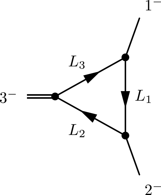
Using the three-point vertex (2.13), the three-minus one-loop vertex is proportional to the following integral:

$${\cal T}:=\int\!{d^{D}L\over(2\pi)^{D}}{[\eta|L_{1}|1\rangle[\eta|L_{2}|2\rangle[\eta|L_{3}|3\rangle\over[\eta 1][\eta 2][\eta 3]}\cdot{1\over L_{1,D}^{2}L_{2,D}^{2}L_{3,D}^{2}}\ .$$ (3.1)

We will keep leg 3 off shell, so that the spinors associated to that leg are defined via the lightcone off-shell continuation (2.14). Notice also that we keep the propagators $D$-dimensional.

Let us focus on the quantity444As remarked earlier, we could equivalently write $l_{1}$ and $l_{2}$ in place of $L_{1}$ and $L_{2}$ in (3.1). We choose to keep $L_{1}$ and $L_{2}$ in order to simplify the $D$-dimensional Passarino-Veltman reductions to be performed later.

$$\Sigma:={[\eta|L_{1}|1\rangle[\eta|L_{2}|2\rangle\over[\eta 1][\eta 2]}\ ,$$ (3.2)

which appears in (3.1). As in [23, 24], we write

$${[\eta|L_{1}|1\rangle[\eta|L_{2}|2\rangle\over[\eta 1][\eta 2]}={[\eta|\hat{L}_{1}\hat{k}_{1}\hat{k}_{2}\hat{L}_{1}|\eta]\over[\eta 1][\eta 2][12]}\ ,$$ (3.3)

where we have used $L_{2}=L_{1}-k_{2}$ and $\hat{k}_{2}^{2}=0$. Note that $\hat{L}_{1}\hat{1}=-\hat{1}\hat{L}_{1}+2(k_{1}\cdot L_{1})$, $\hat{2}\hat{L}_{1}=-\hat{L}_{1}\hat{2}+2(k_{2}\cdot L_{1})$ and $L_{2}^{2}=L_{1}^{2}-2(L_{1}\cdot k_{2})$. Hence, we find that $2(l_{1}\cdot k_{2})=L_{1}^{2}-L_{2}^{2}$ and $2(l_{1}\cdot k_{1})=L_{4}^{2}-L_{1}^{2}$. Using these relations we arrive at

$$\Sigma=-L_{1}^{2}{[12]\over\langle 12\rangle}+(L_{3}^{2}-L_{1}^{2}){[\eta|L_{1}|2\rangle\over[\eta 1]}+(L_{2}^{2}-L_{1}^{2}){[\eta|L_{1}|1\rangle\over[\eta 2]}\ .$$ (3.4)

We remark that the spinor algebra from the MHV vertices is four-dimensional, but the propagators are $D$-dimensional.555We would like to point out that, in the integration measure derived in [5], the propagators are also written explicitly in $D$-dimensions. This is why the phase-space integrals appearing in that paper are also $D$-dimensional. Note that

$${L^{2}\over L_{D}^{2}}={L^{2}-\mu^{2}+\mu^{2}\over L_{D}^{2}}=1+{\mu^{2}\over L_{D}^{2}}\ ,$$ (3.5)

i.e. incomplete cancellations of propagators have to be properly taken into account. In supersymmetric theories this is not needed, at least at one loop, due to four-dimensional cut-constructibility [25]. However, for the non-supersymmetric amplitude we are focussing on now, it is crucial to keep track of terms such as $\mu^{2}/L_{D}^{2}$ in (3.5). It is precisely these terms that will give rise to the correct amplitudes; in other words, the result of a calculation for the (finite) all-minus amplitude fully performed in four dimensions would naïvely be zero.

Such an incomplete cancellation happens for the first term in (3.4), where we use $L_{1}^{2}=L_{1,D}^{2}+\mu^{2}$. On the other hand, we can rewrite $L_{2}^{2}-L_{1}^{2}=L_{2,D}^{2}-L_{1,D}^{2}$, as the $\mu^{2}$ terms cancel, as well as $L_{3}^{2}-L_{1}^{2}=L_{3,D}^{2}-L_{1,D}^{2}$. Therefore, we find

$$\Sigma=-\mu^{2}{\langle 12\rangle\over[12]}+{X\over[12]}\ ,$$ (3.6)

where

$$X:=L_{1,D}^{2}{[\eta|L_{3}(k_{1}+k_{2})|\eta]\over[\eta 1][\eta 2]}+L_{3,D}^{2}{[\eta|L_{1}|2\rangle\over[\eta 1]}+L_{2,D}^{2}{[\eta|L_{1}|1\rangle\over[\eta 2]}\ .$$ (3.7)

Notice the presence of the $\mu^{2}$ term in (3.6).

Using (3.6), we can write ${\cal T}$ in (3.1) as

$${\cal T}={\cal T}_{A}+{\cal T}_{B}\ ,$$ (3.8)

where

$${\cal T}_{A}:=\int\!{d^{D}L\over(2\pi)^{D}}\Big{(}-\mu^{2}{\langle 12\rangle\over[12]}{[\eta|L_{3}|3\rangle\over[\eta 3]}\Big{)}\cdot{1\over L_{1,D}^{2}L_{2,D}^{2}L_{3,D}^{2}}\ ,$$ (3.9)

and

$${\cal T}_{B}:=\int\!{d^{D}L\over(2\pi)^{D}}\Big{(}{X\over[12]}{[\eta|L_{3}|3\rangle\over[\eta 3]}\Big{)}\cdot{1\over L_{1,D}^{2}L_{2,D}^{2}L_{3,D}^{2}}\ .$$ (3.10)

We first focus on ${\cal T}_{A}$, and recast it as

$${\cal T}_{A}={i\over(4\pi)^{2-\epsilon}}\,I[\mu^{2};L_{3\nu}]{\langle 12\rangle\over[12]}{[\eta|\nu|3\rangle\over[\eta 3]}\ ,$$ (3.11)

where $I[\mu^{2};L_{3\nu}]$ is a one-mass vector triangle integral666We summarise our notation and results for integrals in Appendix C.. It is given by

$$I[\mu^{2};L_{3\nu}]=\Big{(}-J_{3}(k_{3}^{2})+2{J_{2}(k_{3}^{2})\over k_{3}^{2}}\Big{)}k_{2\nu}+\Big{(}-{J_{2}(k_{3}^{2})\over k_{3}^{2}}-J_{3}(k_{3}^{2})\Big{)}k_{3\nu}\ .$$ (3.12)

Substituting this into (3.9), we find

$${\cal T}_{A}={i\over(4\pi)^{2-\epsilon}}\,{\langle 12\rangle\over[12]}{[\eta|2|3\rangle\over[\eta 3]}\Big{(}-J_{3}(k_{3}^{2})+2{J_{2}(k_{3}^{2})\over k_{3}^{2}}\Big{)}\ .$$ (3.13)

Furthermore, it is easy to see that ${\cal T}_{B}=0$. Indeed, ${\cal T}_{B}$ is a sum of three two-tensor bubble integrals, each of which separately vanishes due to the spinor contractions.

Therefore, the final result for the three-point vertex is

$$V_{3}(\epsilon)\ =\ {i\over(4\pi)^{2-\epsilon}}\,{\langle 12\rangle\over[12]}{[\eta|2|3\rangle\over[\eta 3]}\Big{(}-J_{3}(k_{3}^{2})+2{J_{2}(k_{3}^{2})\over k_{3}^{2}}\Big{)}\ ,$$ (3.14)

where $k_{3}$ is the off-shell leg, $k_{3}^{2}\neq 0$. It is illuminating to take the $\epsilon\to 0$ limit of (3.14). Since $J_{3}(k_{3}^{2})\to-1/2$, $J_{2}\to-k_{3}^{2}/6$ in this limit, we get

$$V_{3}={i\over 96\pi^{2}}{\langle 12\rangle\over[12]}{[\eta|2|3\rangle\over[\eta 3]}\ .$$ (3.15)

3.1 The one-loop splitting amplitude from the one-loop vertex

As a quick application of the result (3.15) for the four-dimensional limit of the three-point all-minus vertex we can re-derive the one-loop splitting amplitude $S_{-}(a^{-},b^{-})$ with one real scalar running in the loop [26, 27].

To proceed we consider our previous result (3.15),

$$V_{3}={i\over 96\pi^{2}}{\langle ab\rangle\over[ab]}{[\eta|b|k\rangle\over[\eta k]}\ ,$$ (3.16)

where $k=-(k_{a}+k_{b})$. In the limit where $k_{a}$ and $k_{b}$ become collinear we set, as usual, $k_{a}\to zk$, $k_{b}\to(1-z)k$, and take $k^{2}\to 0$. Then we rewrite

$${[\eta|b|k\rangle\over[\eta k]}={\langle ak\rangle\langle kb\rangle\over\langle ab\rangle}=\langle ab\rangle{[a\eta][b\eta]\over[k\eta]^{2}}\ ,$$ (3.17)

where in the first equality we multiplied and divided by $\langle kb\rangle$, and in the second by $[k\eta]^{2}$. The derivation of the splitting amplitude is similar to that of the tree-level splitting amplitude for the helicity configuration $--\to-$ considered in [4], where the splitting amplitude is obtained by multiplying a vertex by a propagator $1/k^{2}$. Doing this, we obtain

$$S_{-}(a^{-},b^{-})={i\over 96\pi^{2}}{\langle ab\rangle\over\,\,[ab]^{2}}{[a\eta][b\eta]\over[k\eta]^{2}}\ .$$ (3.18)

Finally replacing $k_{a}\to zk$, $k_{b}\to(1-z)k$ we get

$$S_{-}(a^{-},b^{-})(z)\ =\ {i\over 96\pi^{2}}\sqrt{z(1-z)}{\langle ab\rangle\over\,\,[ab]^{2}}\ =\ {i\over 96\pi^{2}}\,\sqrt{z(1-z)}{\langle ab\rangle\over\,\,[ab]^{2}}\ ,$$ (3.19)

in agreement with the result of [26, 27].

4 The four-point all-minus amplitude

In order to calculate the four-point all-minus amplitude, we will have to sum diagrams with three different topologies, namely a box diagram, diagrams containing a three-point all-minus vertex, and finally bubble-like diagrams. The box diagram is depicted in figure 2, while the other two topologies can be found in figure 3. We will see that the box diagrams contains the correct result for the amplitude, plus additional terms which will be cancelled by the diagrams containing a three-minus vertex. The bubble-like diagrams will be seen to vanish. In the following we present a detailed analysis of these contributions.

4.1 The box diagram

Refer to caption
Figure 2: The box MHV-diagram contributing to the all-minus four-gluon amplitude. A complex scalar runs in the loop, and one has to sum over the two possible internal helicity assignments. This has the effect of doubling the result of a single internal helicity assignment.

This diagram is depicted in figure 2, and its expression is

$${\cal B}=\int\!{d^{D}L\over(2\pi)^{D}}{[\eta|L_{1}|1\rangle[\eta|L_{2}|2\rangle[\eta|L_{3}|3\rangle[\eta|L_{4}|4\rangle\over[\eta 1][\eta 2][\eta 3][\eta 4]}{1\over L_{1,D}^{2}L_{2,D}^{2}L_{3,D}^{2}L_{4,D}^{2}}\ .$$ (4.1)

Manipulations similar to those which led to (3.6) allow us to rewrite

$${[\eta|L_{1}|1\rangle[\eta|L_{2}|2\rangle\over[\eta 1][\eta 2]}=-\mu^{2}{\langle 12\rangle\over[12]}+{X\over[12]}\ ,$$ (4.2)

where

$$X=L_{1,D}^{2}{[\eta|L_{4}(1+2)|\eta]\over[\eta 1][\eta 2]}+L_{4,D}^{2}{[\eta|L_{1}|2\rangle\over[\eta 1]}+L_{2,D}^{2}{[\eta|L_{1}|1\rangle\over[\eta 2]}\ ,$$ (4.3)

and

$${[\eta|L_{3}|3\rangle[\eta|L_{4}|4\rangle\over[\eta 3][\eta 4]}=-\mu^{2}{\langle 34\rangle\over[34]}+{Y\over[34]}\ ,$$ (4.4)

where

$$Y=L_{3,D}^{2}{[\eta|L_{2}(3+4)|\eta]\over[\eta 3][\eta 4]}+L_{2,D}^{2}{[\eta|L_{3}|4\rangle\over[\eta 3]}+L_{4,D}^{2}{[\eta|L_{3}|3\rangle\over[\eta 4]}\ .$$ (4.5)

Therefore, the integrand in (4.1) becomes

$${N\over L_{1,D}^{2}L_{2,D}^{2}L_{3,D}^{2}L_{4,D}^{2}}\ ,$$ (4.6)

with

$$N=\Big{(}-\mu^{2}{\langle 12\rangle\over[12]}+{X\over[12]}\Big{)}\Big{(}-\mu^{2}{\langle 34\rangle\over[34]}+{Y\over[34]}\Big{)}\ .$$ (4.7)

Thus we are led to consider the following four integrals:

$\displaystyle{\cal B}_{1}$ $\displaystyle=$ $\displaystyle\int\!{d^{D}L\over(2\pi)^{D}}{\mu^{4}\over L_{1,D}^{2}L_{2,D}^{2}L_{3,D}^{2}L_{4,D}^{2}}{\langle 12\rangle\langle 34\rangle\over[12][34]}\ ,$ (4.8)
$\displaystyle{\cal B}_{2}$ $\displaystyle=$ $\displaystyle-{\langle 12\rangle\over[12][34]}\int\!{d^{D}L\over(2\pi)^{D}}{\mu^{2}Y\over L_{1,D}^{2}L_{2,D}^{2}L_{3,D}^{2}L_{4,D}^{2}}\ ,$ (4.9)
$\displaystyle{\cal B}_{3}$ $\displaystyle=$ $\displaystyle{\cal B}_{2}\big{(}(1,2)\leftrightarrow(3,4)\big{)}\ ,$ (4.10)
$\displaystyle{\cal B}_{4}$ $\displaystyle=$ $\displaystyle{\langle 12\rangle\langle 34\rangle\over[12][34]}\int\!{d^{D}L\over(2\pi)^{D}}{XY\over L_{1,D}^{2}L_{2,D}^{2}L_{3,D}^{2}L_{4,D}^{2}}\ .$ (4.11)

The first one can be evaluated immediately:

$${\cal B}_{1}\ =\ {i\over(4\pi)^{2-\epsilon}}\,{\langle 12\rangle\langle 34\rangle\over[12][34]}I_{4}^{4-2\epsilon}[\mu^{4}]\ =\ {i\over(4\pi)^{2-\epsilon}}\,K_{4}\,{\langle 12\rangle\langle 34\rangle\over[12][34]}\ ,$$ (4.12)

where $K$ is defined in (C.3).

We will see that (4.12) is actually the final result of the calculation, as all the additional contributions will cancel out in the final expression. In the $\epsilon\to 0$ limit, the integral function $K$ is finite, see (C.4).

From this equation it is also clear that, in dimensional regularisation, the finiteness of the all-minus amplitude emerges from an $\epsilon\times 1/\epsilon$ cancellation, where the $\epsilon$ factor is due to $\mu^{2}$ factors in the numerator of the integrand and the $1/\epsilon$ is due to the loop integration. As such, it is intriguing to speculate [28] that one may be able to interpret this amplitude as an anomaly.

The evaluation of the remaining integrals in (4.8) is less immediate, and requires extensive use of PV reductions. Here we will only quote the final result for the different expressions. We find777In the following expressions for the ${\cal B}$’s we will omit an ubiquitous prefactor of $i/(4\pi)^{2-\epsilon}$.

$${\cal B}_{2}+{\cal B}_{3}={([\eta|12|\eta]+[\eta|34|\eta])^{2}\over[12][34]\prod_{i=1}^{4}[\eta i]}{J_{2}(t)\over t}\,+\,{[\eta|12|\eta]^{2}+[\eta|34|\eta]^{2}\over[12][34]\prod_{i=1}^{4}[\eta i]}\bigg{(}-J_{3}(s)+{2\over s}J_{2}(s)\bigg{)}\ ,$$ (4.13)

and

$${\cal B}_{4}={[\eta|23|\eta]^{2}+[\eta|41|\eta]^{2}\over[23][41]\prod_{i=1}^{4}[\eta i]}\,\bigg{(}-J_{3}(t)+{2\over t}J_{2}(t)\bigg{)}\,-\,{([\eta|23|\eta]+[\eta|41|\eta])^{2}\over[12][34]\prod_{i=1}^{4}[\eta i]}{J_{2}(t)\over t}\ .$$ (4.14)

Cancellation of the $J_{2}(t)$ terms in (4.13) and (4.14) occurs thanks to the identity $[\eta|23+41-12-34|\eta]=0$, and we are left with the following contribution from the box diagram:

$\displaystyle\sum_{i=1}^{4}{\cal B}_{i}$ $\displaystyle=$ $\displaystyle K_{4}\,{\langle 12\rangle\langle 34\rangle\over[12][34]}+{[\eta|12|\eta]^{2}+[\eta|34|\eta]^{2}\over[12][34]\prod_{i=1}^{4}[\eta i]}\bigg{(}-J_{3}(s)+{2\over s}J_{2}(s)\bigg{)}\,$
$\displaystyle+$ $\displaystyle\,{[\eta|23|\eta]^{2}+[\eta|41|\eta]^{2}\over[23][41]\prod_{i=1}^{4}[\eta i]}\,\bigg{(}-J_{3}(t)+{2\over t}J_{2}(t)\bigg{)}\ .$

4.2 The triangle diagrams

In this section we consider the diagrams containing the one-loop three-point vertex we calculated earlier, with the off-shell leg connected to a tree-level, three-point MHV vertex. There are four such diagrams, one of which is depicted in figure 3. The other three diagrams are obtained by cyclic permutation of the external particles. These diagrams can be evaluated using our expression (3.14) for the three-point vertex, and the $--+$ vertex. After a little algebra, one finds that the triangle diagram in figure 3 gives

$${\cal T}_{1}\ =\ -{[\eta|34|\eta]^{2}\over[12][34]\prod_{i=1}^{4}[\eta i]}\bigg{(}-J_{3}(s)+{2\over s}J_{2}(s)\bigg{)}\ ,$$ (4.16)

and hence the sum over the four cyclic permutations gives

$$\sum_{i=1}^{4}{\cal T}_{1}\ =\ -{[\eta|12|\eta]^{2}+[\eta|34|\eta]^{2}\over[12][34]\prod_{i=1}^{4}[\eta i]}\bigg{(}-J_{3}(s)+{2\over s}J_{2}(s)\bigg{)}\,-\,{[\eta|23|\eta]^{2}+[\eta|41|\eta]^{2}\over[23][41]\prod_{i=1}^{4}[\eta i]}\,\bigg{(}-J_{3}(t)+{2\over t}J_{2}(t)\bigg{)}\ .$$ (4.17)

Notice that when we sum the contribution of the triangle diagrams (4.17) to that of the boxes (4.1), only the $K_{4}$ contribution survives, and we are left with

$$\sum_{i=1}^{4}{\cal B}_{i}+\sum_{i=1}^{4}{\cal T}_{1}\ =\ K_{4}\,{\langle 12\rangle\langle 34\rangle\over[12][34]}\ ,$$ (4.18)

which agrees with the expected result for the all-orders in $\epsilon$ result for the four-point all-minus amplitude. Next we have to consider diagrams which contain a one-loop bubble sub-diagram.

Refer to captionRefer to captionRefer to captionmissing-subexpressionRefer to caption\begin{array}[]{lcr}\scalebox{0.3}{\includegraphics{bubblediagram}}&&\scalebox{0.3}{\includegraphics{trianglediagram}}\end{array}

Figure 3: Bubble and triangle diagrams contributing to the all-minus four-gluon amplitude. The bubble diagram is found to be zero. We also have to include three more triangle diagrams, obtained from the one in the figure by cyclically rotating the external particles.

4.3 The bubble diagram

Finally we evaluate two bubble diagrams one of which is depicted in figure 3. The bubble diagram from figure 3 gives

$$\int\!{d^{D}L\over(2\pi)^{D}}\,{1\over L_{1,D}^{2}L_{2,D}^{2}}\,\Big{(}{[\eta|L_{1}|k\rangle\over[\eta k]}\Big{)}^{2}\ ,$$ (4.19)

where $k$ is the lightcone truncation of $K_{12}:=k_{1}+k_{2}$. The integral (4.19) is proportional to a two-tensor bubble integral

$$\int\!{d^{D}L\over(2\pi)^{D}}\,{L_{1}^{\mu}\,L_{1}^{\nu}\over L_{1,D}^{2}L_{2,D}^{2}}\ ,$$ (4.20)

whose expression is given in Appendix C. However, the explicit expression is not needed. On general grounds the tensor bubble is a linear combination of $\eta^{\mu\nu}$ and $K_{12}^{\mu}K_{12}^{\nu}$. Both tensor structures contract to zero when inserted into (4.19). Since the other bubble diagram obtained by cyclic permutation of the external lines is also zero, this class of diagrams gives a vanishing contribution.

5 A holomorphic field redefinition

In this section we consider a particular holomorphic change of variables in the Yang-Mills path integral,888Also recently studied in [29]. which is different from the canonical field redefinition of Mansfield [21]. The special form of the Chalmers-Siegel Lagrangian (A.11), which we write here for convenience as

$${\cal L}_{\rm CS}:={1\over 2}\bar{A}\Big{(}\square\,A+2i[\partial^{-}A,\partial^{z}A]\Big{)}\ ,$$ (5.1)

suggests the choice of a new set of variables $(B,\bar{B})$, where $\bar{B}=\bar{A}$ and $B$ is a function of $A$ alone such that the Lagrangian is free, when written in terms of $(B,\bar{B})$,

$${\cal L}_{\rm CS}:={1\over 2}\bar{B}\square\,B\ .$$ (5.2)

In this sense, this change of variables is similar to the Bäcklund transformations which have been applied to Liouville theory [30].

Equations (5.1) and (5.2) determine $A=A(B)$ to be the solution of

$$\square\,A+2i[\partial^{-}A,\partial^{z}A]\ =\ \square B\ .$$ (5.3)

This change of variables is non-canonical, and only transforms the $A$ fields, leaving the $\bar{A}$ field untouched. Moreover it is holomorphic, $A=A(B)$ so that $B$ has no dependence on the $\bar{A}$ fields. One can solve (5.3) perturbatively,

$$A\ =\ A^{(0)}\,+\,A^{(1)}\,+\,A^{(2)}\,+\,\cdots\ ,$$ (5.4)

where $A^{(0)}=B$, $A^{(1)}=-2i\square^{-1}[\partial^{-}B,\partial^{z}B]$, $\ldots$ In general $A^{(n)}$ contains $n+1$ insertions of the field $B$. Interestingly, the solution of the self-dual Yang-Mills equations of motion can be bootstrapped using a Bethe Ansatz [28, 31, 32] and has intriguing connections to integrability.

If this change of variables is applied to the full Yang-Mills Lagrangian, a full set of MHV-like vertices is generated. One can readily see that these cannot be equal to the known MHV vertices, as derived explicitly in [22] using a non-holomorphic but canonical change of variables. The reason is that certain contributions, that are needed to get the full MHV vertices as in [22], are missing in the expressions obtained from the holomorphic field redefinition. However, one expects the same on-shell expressions, and very recent investigations appear to confirm this [29].

Specifically, the fact that we transform the field $A$ but not $\bar{A}$ has an important consequence. Consider the four-point gluon vertex. In terms of the new fields, it receives two kinds of contributions: a. a contribution from the original four-point vertex in the Lagrangian, where we substitute $\bar{A}=\bar{B}$ and the lowest-order term in the expansion of the solution $A=A(B)$ to (5.3), $A^{(0)}=B$; and b. a contribution from the three-point vertex in the Yang-Mills Lagrangian, of the form (schematically) $\bar{A}\bar{A}A$, where we replace $A$ by the term in the expansion of $A=A(B)$ containing two $B$-fields. The term we generate is thus of the form999A trace over colour is always understood. $BB\bar{B}\bar{B}$. Importantly, this correction alters the vertex with helicities $--++$, but not the split-helicity vertex $-+-+$. This means that the perturbative expansion in terms of the new fields is going to be different from that giving rise to MHV rules.

5.1 The all-plus helicity amplitude from a Jacobian

We now discuss how the new field variables defined above yield the all-plus helicity amplitudes. The holomorphic change of variables is not canonical and leads to a nonvanishing Jacobian

$${\cal J}(B)\ =\ {\rm det_{\it x,y}}\left({\delta A(x)\over\delta B(y)}\right)(B)\ ,$$ (5.5)

which is a functional of the $B$ fields only, and as such can contribute to the all-plus scattering amplitude, obtained from the correlator $\langle\bar{A}(x_{1})\cdots\bar{A}(x_{n})\rangle$ upon application of standard reduction formulae. More precisely, we wish to compute

$$G(x_{1},\ldots,x_{n})\ :=\ \langle\bar{A}(x_{1})\cdots\bar{A}(x_{n})\rangle\ =\ \langle\bar{B}(x_{1})\cdots\bar{B}(x_{n})\,{\cal J}^{(n)}(B)\rangle_{\rm free}\ ,$$ (5.6)

where in the right hand side we perform free Wick contractions of the $B$ and $\bar{B}$ fields, and ${\cal J}^{(n)}(B)$ is the term in the Jacobian (5.5) which contains $n$ $B$ fields.

Now we argue that in this way we precisely obtain the all-plus amplitude, which is missing within the MHV diagram formalism. Our strategy is very simple. We calculate the Jacobian and its contribution to the all-plus correlation function in terms of diagrams (without evaluating them explicitly), and show that these diagrams precisely match those obtained with lightcone quantisation (these are the parity conjugate diagrams of those considered in the all-minus calculation).

This is most easily seen in a toy model, which captures the essence of the problem. In this model, the cubic interaction of self-dual Yang-Mills is replaced by the simpler cubic interaction $\lambda\bar{A}AA$ which is free of derivatives. We consider

$${\cal L}:=\bar{A}(-\square A+\lambda A^{2})\ ,$$ (5.7)

and we redefine fields so that

$${\cal L}=-\bar{B}\square B\ .$$ (5.8)

We use the holomorphic change of variables

$$\bar{A}\ =\ \bar{B}\ ,$$ (5.9)

and

$$-\square A+\lambda A^{2}\ =\ -\square B\ .$$ (5.10)

The three-point vertex of the original Lagrangian is proportional to $-\lambda f^{abc}$ and contributes to the Green function $\langle\bar{A}(x)\bar{A}(y)A(z)\rangle$.

At the level of functional integrals, we have the equalities

$$Z(J,\bar{J}):=\int\!\delta A\delta\bar{A}\ e^{-S(A,\bar{A})+\int\bar{J}A+\int\bar{A}J}=\int\!\delta B\delta\bar{B}\ {\cal J}(B)\,\ e^{-S_{\rm free}(B,\bar{B})+\int\bar{J}A(B)+\int\bar{B}J}\ .$$ (5.11)

Notice the presence of the Jacobian ${\cal J}(B)$ defined in (5.5), and the fact that the source $\bar{J}$ is coupled to $A=A(B)$, i.e. the solution to the change of variables (5.10). Taking a functional derivative of (5.10) with respect to $B$ we get

$$\Big{(}-\square_{x}+2\lambda A(x)\Big{)}{\delta A(x)\over\delta B(y)}=-\square\delta(x-y)\ ,$$ (5.12)

or, formally,

$${\delta A(x)\over\delta B(y)}\ =\ (1-2\lambda\square^{-1}A)^{-1}_{x,y}\ .$$ (5.13)

We have

$\displaystyle{\cal J}$ $\displaystyle:=$ $\displaystyle{\rm det}_{x,y}\left({\delta A(x)\over\delta B(y)}\right)=e^{{\rm Tr}\log(1-2\lambda\square^{-1}A)^{-1}}\ =\ e^{-{\rm Tr}\log(1-2\lambda\square^{-1}A)}$
$\displaystyle=$ $\displaystyle\exp\left[{\sum_{m=1}^{\infty}{1\over m}{\rm Tr}\big{[}(2\lambda\,\square^{-1}A)^{m}\big{]}}\right]\ ,$

where101010(5.15) is meant to be properly regularised, by e.g. using dimensional regularisation.

$${\rm Tr}\big{[}(2\lambda\,\square^{-1}A)^{m}\ =\ (2\lambda)^{m}\int\!d^{4}y_{1}\cdots d^{4}y_{m}\ G(y_{1}-y_{2})A(y_{2})\,G(y_{2}-y_{3})A(y_{3})\cdots G(y_{m}-y_{1})A(y_{1})\ ,$$ (5.15)

and $\square G(x)=\delta^{(4)}(x)$. Our correlator (5.6) becomes then

$\displaystyle G(x_{1},\ldots,x_{n})\ =$ (5.16)
(5.17)
$\displaystyle\left\langle\bar{B}(x_{1})\cdots\bar{B}(x_{n})\,e^{{\sum_{m=1}^{\infty}{(2\lambda)^{m}\over m}\int\!d^{4}y_{1}\cdots d^{4}y_{m}\ G(y_{1}-y_{2})A(y_{2})\,G(y_{2}-y_{3})A(y_{3})\cdots G(y_{m}-y_{1})A(y_{1})}}\right\rangle_{\rm free}\ ,$

where on the right hand side of (5.16) (as well as (5.1)) one should think of $A$ as the functional of the $B$-fields $A=A(B)$ given by the solution of (5.10). Moreover, we need to pick the term in the expansion of the exponential which contains $n$ $B$-fields, as indicated on the right hand side of (5.6).

In order to determine $A=A(B)$, we need to solve (5.10), and we can do that perturbatively. We set

$$A(B)=A^{(0)}+A^{(1)}+A^{(2)}+\cdots\ ,$$ (5.18)

where we find $A^{(0)}=B$, and

$$A^{(1)}=\lambda\,\square^{-1}B^{2}\ ,$$ (5.19)

and so on.

Now we need to perform free Wick contractions in (5.16). If we pick the solution to lowest order, $A^{(0)}=B$, we obtain a contribution proportional to

$$\lambda^{n}\int\!d^{4}y_{1}\cdots d^{4}y_{n}\ G(y_{1}-y_{2})\,G(y_{2}-y_{3})\cdots G(y_{n}-y_{1})\ G(x_{1}-y_{1})\cdots G(x_{n}-y_{n})\ .$$ (5.20)

This is nothing but the $n$-vertex polygon diagram one would draw with the $\lambda\bar{A}AA$ vertex in the original Lagrangian; at four points, it is (the parity conjugate of) the box diagram in the all-minus calculation – the diagram with the maximum number of propagators, $n$.

The diagrams corresponding, in our four-point example, to triangle and bubble topologies, arise by taking precisely one insertion of $A^{(1)}$ and two of $A^{(0)}$, and two insertions of $A^{(1)}$ for the fields $A$ appearing on the right hand side of (5.16), respectively. Let us check this in more detail for the triangle diagram in the four-point case. The corresponding contribution is proportional to

$\displaystyle\lambda^{4}\int\!d^{4}y_{1}d^{4}y_{2}d^{4}y_{3}\ G(y_{1}-y_{2})\,G(y_{2}-y_{3})G(y_{3}-y_{1})\ G(x_{1}-y_{1})G(x_{2}-y_{2})\,$
$\displaystyle\qquad\qquad\qquad\qquad\square^{-1}_{y_{3}}\left[G(x_{3}-y_{3})G(x_{4}-y_{3})\right]\ ,$ (5.21)

and matches the triangle diagram in figure 3 (we recall that $\square^{-1}_{y}f(y)=\int\!d^{4}z\,G(y-z)f(z)$). Indeed, the insertion of $\square^{-1}$ in (5.1) corresponds to the propagator connecting the tree-level vertex in the figure to the loop, and the two propagators $G(x_{3}-y_{3})G(x_{4}-y_{3})$ are attached to this tree-level three-point vertex. The propagators $G(x_{1}-y_{1})G(x_{2}-y_{2})$ are those emerging from the loop.

The bubble-like diagram would contribute

$$\lambda^{4}\int\!d^{4}y_{1}d^{4}y_{2}\ \square^{-1}_{y_{1}}\left[G(x_{1}-y_{1})G(x_{2}-y_{1})\right]\,\square^{-1}_{y_{2}}\left[G(x_{3}-y_{2})G(x_{4}-y_{2})\right]\ ,$$ (5.22)

again matching the parity conjugated of the bubble-diagram (see figure 3) in the four-minus calculation for the toy model.

The analogous calculation for the self-dual Yang-Mills theory would clearly reproduce the same diagrammatics, and would be expected to give the correct expressions for the amplitudes.

5.2 The single-minus and the single-plus helicity amplitudes

The amplitudes in pure Yang-Mills where all gluons but one have the same helicity are quite special because of their finiteness, a feature in common with the all-plus and the all-minus amplitudes. In this section we would like to sketch how they are calculated within the framework of the holomorphic change of variables introduced above.

The amplitude with a single positive helicity and its parity conjugate, the amplitude with a single negative helicity, have a quite different origin, so we will discuss them separately. In each case, the strategy will be to map the contributions arising from the change of variables to those of lightcone Yang-Mills perturbation theory.

5.2.1 The single-plus amplitude

The $n$-point single-plus amplitude must come from a diagram containing precisely $n-1$ MHV vertices.111111An amplitude with $q$ negative-helicity gluons is built out of $q-1+L$ MHV vertices, where $L$ is the number of loops. The correlation function corresponding to such amplitude is

$$G(x_{1},\ldots,x_{n})\ :=\ \left\langle A(x_{1})\cdots A(x_{n-1})\bar{A}(x_{n})\right\rangle\ ,$$ (5.23)

which we would like to evaluate using the new variables. Here we will limit our attention to the $n$-gon diagram contribution, in the simple case of $n=4$. Generalisation to $n>4$ particles and diagrams with other topologies is straightforward.

The relevant term to study, after re-expressing $G(x_{1},\ldots,x_{n})$ in terms of the new fields, is

$$\Big{\langle}A(x_{1})A(x_{2})A(x_{3})\bar{B}(x_{4})\,\lambda^{3}\int\!\prod_{i=1}^{3}d^{4}z_{i}\ (\bar{B}\bar{B}A)(z_{1})\,(\bar{B}\bar{B}A)(z_{2})\,(\bar{B}\bar{B}A)(z_{3})\,\ {\cal J}(B)\Big{\rangle}_{\rm free}\,,$$ (5.24)

where $A=A(B)$ and the subscript “free” instructs one to take free Wick contractions of the $B$ and $\bar{B}$ fields. Notice that in (5.24) the old fields $A=A(B)$, expressed as functionals of the new fields, are inserted. A naïve application of the equivalence theorem would allow us to replace the old fields by the new ones in a correlation function, without changing the corresponding scattering amplitudes (the correlation function would of course be different). In the case of the holomorphic field redefinition discussed above, the equivalence theorem cannot be applied, because that field redefinition is singular precisely on the mass shell. This issue is discussed in Appendix Acknowledgements.121212The equivalence theorem has a long history. For a back of the envelope proof, see [33]. The issue of a violation of the equivalence theorem using the change of variables discussed here was also recently addressed in [29].

In order to generate a box-diagram structure, we need to open up an extra propagator. This is obtained from taking in any of the three insertions of the functional $A(B)$ (determined by (5.10)) the first nontrivial iteration in the solution $A^{(1)}$, calculated in (5.19), and for the remaining $A$ fields, the zeroth order iteration, $A^{(0)}=B$. A typical term will look like

$\displaystyle\lambda^{4}\Big{\langle}B(x_{1})B(x_{2})B(x_{3})\bar{B}(x_{4})\,\int\!\prod_{i=1}^{3}d^{4}z_{i}\ (\bar{B}\bar{B}B)(z_{1})\,(\bar{B}\bar{B}B)(z_{2})\,$
$\displaystyle\hskip 99.58464pt\times\ (\bar{B}\bar{B})(z_{3})\,\int\!dz^{4}_{4}\,G(z_{3}-z_{4})(BB)(z_{4})\Big{\rangle}_{\rm free}\,.$ (5.25)

Notice that we have picked the zeroth order term in the Jacobian, as well as for the external field $A(B)(x_{4})$. Contracting $B(z_{4})$ with $\bar{B}(z_{1})$, $B(z_{1})$ with $\bar{B}(z_{2})$, and $B(z_{2})$ with $\bar{B}(z_{3})$, we obtain the required box structure, proportional to

$$\lambda^{4}\int\!\prod_{i=1}^{4}d^{4}z_{i}\ G(z_{1}-z_{2})G(z_{2}-z_{3})G(z_{3}-z_{4})G(z_{4}-z_{1})\ .$$ (5.26)

The remaining fields which are integrated over contract in an obvious way with the insertions $B(x_{1})$, $B(x_{2})$, $B(x_{3})$, and $\bar{B}(x_{4})$.

5.2.2 The single-minus amplitude

Finally, let us consider the single-minus helicity amplitude. The relevant correlation function is

$$G(x_{1},\ldots,x_{n})\ :=\ \left\langle\bar{A}(x_{1})\cdots\bar{A}(x_{n-1})A(x_{n})\right\rangle\ .$$ (5.27)

Again, we focus only on the four-point case, and specifically on the box -function contribution. We expect to use a single MHV three-point vertex; the relevant box-like term is obtained from

$$\left\langle\bar{B}(x_{1})\bar{B}(x_{2})\bar{B}(x_{3})A(x_{4})\ \lambda\int\!d^{4}z(\bar{B}\bar{B}A)(z)\,{\cal J}(B)\right\rangle_{\rm free}\ .$$ (5.28)

The box diagram structure clearly comes from considering the $\lambda^{3}$ iteration of the field $A(B)$ which sits inside the $z$-integral. This iteration is schematically of the form

$\displaystyle A^{(3)}$ $\displaystyle\sim$ $\displaystyle\lambda\square^{-1}(A^{(0)}A^{(2)}+A^{(2)}A^{(0)}+A^{(1)}A^{(1)})$
$\displaystyle\sim$ $\displaystyle\lambda^{3}(\square^{-1}B\square^{-1}B\square^{-1}B^{2})\ +\ \lambda^{3}(\square^{-1}B^{2})(\square^{-1}B^{2})\ .$

In order to make a box diagram we need three integrations, so we need to pick the first term in (5.2.2). We rename $z\to z_{1}$ and use

$$(\square^{-1}B\square^{-1}B\square^{-1}B^{2})(z_{1})=\int\!\prod_{i=2}^{4}d^{4}z_{i}\ G(z_{1}-z_{2})B(z_{2})\,G(z_{2}-z_{3})B(z_{3})\,G(z_{3}-z_{4})(BB)(z_{4})\ .$$ (5.30)

The fourth propagator needed to form a box is obtained from contracting $B(z_{4})$ with one of the two $\bar{B}(z_{1})$ in (5.28). Finally, the remaining fields are contracted in an obvious way with the insertions $\bar{B}(x_{1})$, $\bar{B}(x_{2})$, $\bar{B}(x_{3})$, and $B(x_{4})$. The box diagram arises from setting $A(x_{4})\to B(x_{4})$, and from taking the trivial contribution ${\cal J}\to 1$ to the Jacobian.

5.3 Perturbation theory in the new variables

Now consider the question of perturbation theory in the new variables $(B,\bar{B})$. As we have seen there are three types of contributions – those coming directly from the Lagrangian, expressed in terms of the new variables, those coming from the Jacobian, and finally those coming from violations of the equivalence theorem, which express themselves through contributions from field redefinitions of the external states. We have argued that the Jacobian terms alone give rise to the one-loop all-plus amplitudes, while the all-minus is obtained solely from three-point MHV vertices, which are not modified in our holomorphic field redefinition. Our analysis indicates that the single-minus and the single-plus amplitudes arise from combinations of MHV-type vertices with the Jacobian and external state contributions. In general, the procedure for calculating complete amplitudes with generic helicities using these new variables is then clear: one combines the effective vertices from the Lagrangian with the equivalence theorem violating contributions and those arising from the Jacobian.

6 Conclusions

We would like to end with some comments and speculations:

1. Given the fact that the MHV three-point vertices are nothing but the lightcone vertices, the agreement of our MHV diagram calculation with the all orders in $\epsilon$ result for this amplitude will persist for all $n$-point all-minus scattering amplitudes.

2. The fact that the all-minus amplitude is non-zero arises from an $\epsilon\times 1/\epsilon$ cancellation, as we showed explicitly in the calculations of sections 3 and 4. This is reminiscent of an anomaly, as also noted by numerous authors in the context of related calculations [28, 31, 34, 35, 36]. It would be interesting to make this statement more precise, and to understand which symmetry is anomalous.

3. We have explained the all-plus amplitude as coming from a Jacobian. This applies to our holomorphic change of variables, which is different from Mansfield’s canonical transformation [21]. However, it is likely that a proper quantum treatment of Mansfield’s approach would also lead to a Jacobian which then would yield the all-plus amplitude.

4. After arguing that we can derive the all-plus amplitudes, we discussed how to obtain the single negative/positive helicity amplitudes in a toy model which is closely related to the Yang-Mills case. Clearly it would be of interest to do this directly in Yang-Mills.

5. In supersymmetric theories the amplitudes with zero or one particle of one helicity type vanish, due to supersymmetric Ward identities. Thus the Jacobians must cancel in these cases. It would be interesting to show this explicitly.

6. Finally, it is clear that the holomorphic change of variables discussed in section 5 gives a different perturbation theory. But one can ask whether this yields practical rules, or, more precisely, if the perturbative expansion can be reassembled into an effective set of vertices which incorporate equivalence theorem violating contributions and possibly contributions from the Jacobian. This seems to us an interesting avenue to follow.

Acknowledgements

It is a pleasure to thank Zvi Bern, Rutger Boels, Freddy Cachazo, Paul Heslop, Paul Mansfield, Tim Morris, Sanjaye Ramgoolam, Diana Vaman and Costas Zoubos for discussions, and Simon McNamara for collaboration at the initial stage of this project. We would like to thank PPARC for support under a Rolling Grant PP/D507323/1 and the Special Programme Grant PP/C50426X/1. The work of GT is supported by an EPSRC Advanced Fellowship and by an EPSRC Standard Research Grant.

Appendix A: A brief review of lightcone gauge theory

We begin by introducing lightcone coordinates

$$x^{\pm}:={x^{0}\pm x^{3}\over\sqrt{2}}\ ,\qquad x^{\hat{\mu}}:=(x^{2},\ldots,x^{D})\ .$$ (A.1)

In terms of these, the scalar products between two vectors $A$ and $B$ is

$$A\cdot B:=A^{+}B^{-}+A^{-}B^{+}-A^{\hat{\mu}}B^{\hat{\mu}}\ ,$$ (A.2)

where $\hat{\mu}$, $\hat{\nu}=1,2$ and we defined $A^{\hat{\mu}}B^{\hat{\mu}}:=A^{\hat{\mu}}B^{\hat{\nu}}\delta_{\hat{\mu}\hat{\nu}}$.

The lightcone gauge is defined by

$$A^{-}=0\ .$$ (A.3)

Equivalently, we can write the above condition as $\eta\cdot A=0$, where $\eta$ is a constant null vector, chosen to have components $\eta:=(1,0,0,1)$.

In the lightcone gauge, the Yang-Mills Lagrangian is131313In this and the following Lagrangians we will omit an obvious trace over the group generators to simplify the notation.

$\displaystyle{\cal L}_{\rm{YM}}$ $\displaystyle:=$ $\displaystyle-{1\over 4}F_{\mu\nu}F^{\mu\nu}={1\over 2}(\partial^{-}A^{+})^{2}-(\partial^{-}A^{\hat{\mu}})(\partial^{\hat{\mu}}A^{+})-iA^{+}[\partial^{-}A^{\hat{\mu}},A^{\hat{\mu}}]+(\partial^{-}A^{\hat{\mu}})(\partial^{+}A^{\hat{\mu}})$ (A.4)
$\displaystyle-$ $\displaystyle{1\over 4}F_{\hat{\mu}\hat{\nu}}F^{\hat{\mu}\hat{\nu}}\ .$

From this equation it is clear that $A^{+}$ is a Lagrange multiplier, and can be integrated out. This amounts to replacing it by the solution to the equations of motion, which is

$$A^{+}=(\partial^{-})^{2}(\partial^{\hat{\mu}}\partial^{-}A^{\hat{\mu}}+i[A^{\hat{\mu}},\partial^{-}A^{\hat{\mu}}])\ .$$ (A.5)

Plugging the solution back into (A.4), one arrives at

$${\cal L}_{\rm YM}=(\partial^{-}A^{\hat{\mu}})(\partial^{+}A^{\hat{\mu}})-{1\over 4}F_{\hat{\mu}\hat{\nu}}F^{\hat{\mu}\hat{\nu}}+{1\over 2}(\partial^{\hat{\mu}}\partial^{-}A^{\hat{\mu}}-i[\partial^{-}A^{\hat{\mu}},A^{\hat{\mu}}])(\partial^{-})^{2}(\partial^{\hat{\nu}}\partial^{-}A^{\hat{\nu}}-i[\partial^{-}A^{\hat{\nu}},A^{\hat{\nu}}])\ .$$ (A.6)

We now specialise to the four-dimensional case, introducing the two complex combinations

$$A^{z}:={A^{1}+iA^{2}\over\sqrt{2}}\ ,\qquad A^{\bar{z}}:={A^{1}-iA^{2}\over\sqrt{2}}\ ,$$ (A.7)

which are the fields for gluons of positive and negative helicity, respectively. The change of variables (A.7) leads to a remarkable simplification in the structure of the four-dimensional Yang-Mills Lagrangian, converting (A.6) into

$${\cal L}:={\cal L}_{-+}+{\cal L}_{-++}+{\cal L}_{+--}+{\cal L}_{--++}\ ,$$ (A.8)

where ${\cal L}_{-+}=-A_{\bar{z}}\square A_{z}$ is the free term, with $\square:=2(\partial_{+}\partial_{-}-\partial_{z}\partial_{\bar{z}})$, and

$\displaystyle{\cal L}_{-++}$ $\displaystyle=$ $\displaystyle 2i[A_{z},\partial_{+}A_{\bar{z}}](\partial_{+})^{-1}(\partial_{\bar{z}}A_{z})\ ,$ (A.9)
$\displaystyle{\cal L}_{+--}$ $\displaystyle=$ $\displaystyle 2i[A_{\bar{z}},\partial_{+}A_{z}](\partial_{+})^{-1}(\partial_{z}A_{\bar{z}})\ ,$
$\displaystyle{\cal L}_{--++}$ $\displaystyle=$ $\displaystyle-2[A_{\bar{z}},\partial_{+}A_{z}](\partial_{+})^{-2}[A_{z},\partial_{+}A_{\bar{z}}]\ .$

This form of the Yang-Mills Lagrangian precisely agrees with that in Eq. 7 of [37].141414After replacing $\square\to-\square$ because of different conventions for the metric, and multiplying their Lagrangian by an overall factor of -2. We also remark that the combination

$${\cal L}_{\rm SDYM}:={\cal L}_{-+}+{\cal L}_{-++}$$ (A.10)

describes the self-dual truncation of pure Yang-Mills theory (the combination ${\cal L}_{-+}+{\cal L}_{--+}$ describes the anti-self-dual truncation).

Upon making the change of variables $\phi:=(\partial^{-})^{-1}A_{z}$, $G^{z-}:=-2\partial^{-}A_{\bar{z}}$, it becomes

$${\cal L}_{\rm CS}:={1\over 2}G^{z-}\Big{(}\square\,\phi+2i[\partial^{-}\phi,\partial^{z}\phi]\Big{)}\ ,$$ (A.11)

which is the Chalmers-Siegel Lagrangian for self-dual Yang-Mills [38]. This is easily derived in a first-order formulation, i.e. by starting from ${\cal L}:=(1/2)G_{\mu\nu}F^{\mu\nu}$, where $G_{\mu\nu}$ is an anti-self-dual field strength, and further imposing the lightcone gauge condition (A.3).

Appendix B: On the equivalence theorem

The purpose of this appendix is to show that when we “redefine away” the three-point vertex in the Chalmers-Siegel Lagrangian (5.1) via the holomorphic change of variables defined by $\bar{B}=\bar{A}$, and $\square A+2i[\partial^{-}A,\partial^{z}A]=\square B$, the three-point interaction reappears as a violation of the equivalence theorem. This theorem can be briefly stated as follows. Consider a theory defined by an action $S(\phi)$ and functional integral

$$Z(J)\ :=\ \int\!\delta\phi\ e^{-S(\phi)+\int\!dx\,J(x)\phi(x)}\ .$$ (B.1)

Now consider a different functional integral

$$\tilde{Z}(J)\ :=\ \int\!\delta\phi\ e^{-S(\phi)+\int\!dx\,J(x)\varphi(\phi)(x)}\ ,$$ (B.2)

where $\varphi:=\varphi(\phi)$ are new fields defined by an invertible change of variables, with $\varphi(\phi)=c\phi+{\cal O}(\phi^{2})$, and $c$ is a constant different from zero. The Green functions obtained from (B.1) and (B.2) are clearly different. However, if $\varphi=\varphi(\phi)$ are good interpolating fields for the quanta carried by $\phi$, scattering amplitudes of the theories (B.1) and (B.2) are identical modulo a wave-function renormalisation, which compensates a possible non-canonical normalisation of the new fields.

Notice finally that one could recast (B.2) as an integral over the new fields,

$$\tilde{Z}(J)\ :=\ \int\!\delta\varphi\ \left|\left|{\delta\phi\over\delta\varphi}\right|\right|\,e^{-\tilde{S}(\varphi)+\int\!dx\,J(x)\varphi(x)}\ ,$$ (B.3)

where $\tilde{S}(\varphi):=S(\phi(\varphi))$ is the action in terms of the new fields.

We now consider the issue of a possible violation of the equivalence theorem using our toy model, defined by the action

$${\cal L}:=\bar{A}(-\square A+\lambda A^{2})\ .$$ (B.4)

We then redefine fields holomorphically using (5.9) and (5.10), so that

$${\cal L}=-\bar{B}\square B\ .$$ (B.5)

Now we would like to calculate at tree level the correlator,

$$\langle\bar{A}(x)\bar{A}(y)A(z)\rangle={\delta^{3}Z\over\delta J(x)\delta J(y)\delta\bar{J}(z)}\ ,$$ (B.6)

which we evaluate using the new-fields representation of the functional integral $Z$ defined in (5.11). If we could apply the equivalence theorem, we would be able to replace $A(B)$ with $B$ on the right hand side of (5.11). This would lead to the wrong conclusion that the Green function (B.6) vanishes because the action $S_{\rm free}(B,\bar{B})$ is free. Instead we use the expansion of the old field $A$ as a function of $B$ as in (5.18), and find

$$\langle\bar{A}(x)\bar{A}(y)A(z)\rangle\ =\ \langle\bar{B}(x)\bar{B}(y)\lambda\square^{-1}B^{2}(z)\rangle_{\rm free}\,+\,\langle\bar{B}(x)\bar{B}(y)B(z)\,2\lambda{\rm Tr}(\square^{-1}B)\rangle_{\rm free}\ .$$ (B.7)

The first term on the right hand side of (B.7) comes from the fact that the sources are coupled to the old fields. The equivalence theorem would imply that its contribution to the correlator is nonzero, but vanishes upon LSZ reduction i.e. does not contribute to the scattering amplitude. The second term comes from a nontrivial Jacobian. The Jacobian term contains a trace which must be properly regularised (it entails an integral over positions). However the trace is also over colour, hence it gives either zero or a subleading term in the large-$N$ limit. We will discard it.151515Moreover, it is a loop effect, and we are now focussing our attention only on the tree-level contribution to (B.6). The first term is nonvanishing and we get (we omit an $f^{abc}$ in front):

$\displaystyle\langle\bar{A}(x)\bar{A}(y)A(z)\rangle$ $\displaystyle=$ $\displaystyle\lambda\,\square^{-1}_{z}\Big{(}G(z-x)G(z-y)\Big{)}$
$\displaystyle=$ $\displaystyle\lambda\int\!d^{4}t\ G(x-t)G(y-t)G(z-t)\ ,$

where $G(x)$ is a free scalar propagator. This is the term which, according to the equivalence theorem, should contribute zero to the scattering amplitude. This is clearly not the case here. To obtain the contribution to the scattering amplitude, we apply LSZ reduction. The first step consists in amputating propagators on the external legs. This is achieved by multiplying $\langle\bar{A}(x)\bar{A}(y)A(z)\rangle$ by $\square_{x}\square_{y}\square_{z}$. We get

$$\square_{x}\square_{y}\square_{z}\ \langle\bar{A}(x)\bar{A}(y)A(z)\rangle=\lambda\,\delta(x-z)\delta(y-z)\ .$$ (B.9)

In the second step we multiply by the wave-functions of free particles, $\exp(ip_{1}x+ip_{2}y+ip_{3}z)$, setting $p_{1}^{2}=p_{2}^{2}=p_{3}^{2}=0$, and Fourier transform in $x,y,z$. The resulting three-point scattering amplitude is

$$\lambda\,\int\!d^{4}x\,d^{4}y\,d^{4}z\ \delta(x-z)\delta(y-z)e^{ip_{1}x+ip_{2}y+ip_{3}z}\ =\ \lambda\ (2\pi)^{4}\delta^{(4)}(p_{1}+p_{2}+p_{3})\ .$$ (B.10)

This is nonvanishing when $p_{1}^{2}=p_{2}^{2}=p_{3}^{2}=0$, and is precisely the contribution of the tree-level three-point vertex in the original Lagrangian for the $A$ and $\bar{A}$ fields.

Our final remark is that this violation of the equivalence theorem is entirely expected. Indeed, starting from the canonically normalised field $A$, the transformation (5.10) is singular, in the sense that it involves the operator $\square^{-1}$, which is singular precisely on the mass shell, where scattering amplitudes are computed. Hence, the field redefinition $A=A(B)$ in (5.10) cannot be compensated simply by a wave-function renormalisation (equivalently, the fields $B$, $\bar{B}$ are not good interpolating fields for the quanta carried by $A$, $\bar{A}$).

Appendix C: Integrals

For convenience, we here summarise some integrals used in this paper.

The scalar $n$-point integral functions in $D=4+2m-2\epsilon$ dimensions are defined as

$\displaystyle I^{D}_{n}\equiv I^{D}_{n}[1]$ $\displaystyle=$ $\displaystyle i(-1)^{n+1}(4\pi)^{D/2}\int\frac{d^{D}L}{(2\pi)^{D}}\frac{1}{L^{2}(L-p_{1})^{2}\cdots(L-\sum_{i=1}^{n-1}p_{i})^{2}}$
$\displaystyle=$ $\displaystyle\frac{i(-1)^{n+1}}{\pi^{2+m-\epsilon}}\int\frac{d^{4+2m}l\,d^{-2\epsilon}\mu}{(l^{2}-\mu^{2})((l-p_{1})^{2}-\mu^{2})\cdots((l-\sum_{i=1}^{n-1}p_{i})^{2}-\mu^{2})}\ .$

The higher dimensional integral functions are related to $4-2\epsilon$ dimensional integrals with a factor $\mu^{2m}$ inserted in the integrand. For $m=1,2$ one finds

$\displaystyle I_{n}[\mu^{2}]\equiv J_{n}$ $\displaystyle=$ $\displaystyle(-\epsilon)I_{n}^{6-2\epsilon}\ ,$ (C.2)
$\displaystyle I_{n}[\mu^{4}]\equiv K_{n}$ $\displaystyle=$ $\displaystyle(-\epsilon)(1-\epsilon)I_{n}^{8-2\epsilon}\,.$ (C.3)

We encounter bubble functions with $m=0,1$, triangles with one massive external line and $m=0,1$, and boxes with four massless external lines and $m=0,1,2$:

$\displaystyle I_{2}(P^{2})\ =\ \frac{r_{\Gamma}}{\epsilon(1-2\epsilon)}(-P^{2})^{-\epsilon}\,\,,\qquad I_{2}^{6-2\epsilon}(P^{2})\ =\ -\frac{r_{\Gamma}}{2\epsilon(1-2\epsilon)(3-2\epsilon)}(-P^{2})^{1-\epsilon}\,\,,$
$\displaystyle I_{3}(P^{2})\ =\ \frac{r_{\Gamma}}{\epsilon^{2}}(-P^{2})^{-1-\epsilon}\qquad\,\,,\qquad I_{3}^{6-2\epsilon}(P^{2})\ =\ \frac{r_{\Gamma}}{2\epsilon(1-\epsilon)(1-2\epsilon)}(-P^{2})^{-\epsilon}\,\,,$
$\displaystyle(-\epsilon)I_{4}^{6-2\epsilon}\ =\ 0+\mathcal{O}(\epsilon)\,\,,\qquad(-\epsilon)(1-\epsilon)I_{4}^{8-2\epsilon}\ =\ -\frac{1}{6}+\mathcal{O}(\epsilon)\,\,.$ (C.4)

Note that the expressions for the bubbles and triangles are valid to all orders in $\epsilon$.

Refer to captionRefer to captionRefer to captionmissing-subexpressionRefer to caption\begin{array}[]{lcr}\scalebox{0.3}{\includegraphics{bubble}}&&\scalebox{0.3}{\includegraphics{triangle}}\end{array}

Figure 4: Kinematics of the bubble and triangle integral functions studied in this appendix.

We now present the result of the PV reduction for various tensor integrals. These are given in terms of scalar $n$-point integral functions $I_{n}^{D}$ in various dimensions $D$, specifically in terms of $I_{n}$, $I_{n}^{6-2\epsilon}$ and $I_{n}^{8-2\epsilon}$ in $4-2\epsilon$, $6-2\epsilon$ and $8-2\epsilon$ dimensions, respectively. The expressions are valid to all orders in $\epsilon$, if $I_{n}$, $I_{n}^{6-2\epsilon}$ and $I_{n}^{8-2\epsilon}$ are evaluated to all orders, and the PV reductions have been performed in a fashion that naturally leads to coefficients without explicit $\epsilon$ dependence (the reader may consult [39] for more details on this particular variant of PV reductions).

For the linear and two-tensor bubbles (Figure 4) we have

$\displaystyle I_{2}\big{[}L^{\mu}\big{]}\ =\ -\frac{1}{2}I_{2}P^{\mu}\ ,$ (C.5)
$\displaystyle I_{2}\big{[}L^{\mu}L^{\nu}\big{]}\ =\ -\frac{1}{2}I_{2}^{6-2\epsilon}\delta^{\mu\nu}_{[4-2\epsilon]}+\bigg{(}\frac{1}{4}I_{2}+\frac{1}{2t}I_{2}^{6-2\epsilon}\bigg{)}P^{\mu}P^{\nu}\ .$ (C.6)

For the linear, two- and three-tensor triangles (Figure 3) we have

$\displaystyle I_{3}\big{[}L_{3}^{\mu}\big{]}\ =\ -\frac{1}{t}I_{2}p_{2}^{\mu}+\bigg{(}-I_{3}+\frac{1}{t}I_{2}\bigg{)}p_{3}^{\mu}\ ,$ (C.7)
$\displaystyle I_{3}\big{[}L_{3}^{\mu}L_{3}^{\nu}\big{]}\ =\ \frac{1}{2t}I_{2}p_{2}^{\mu}p_{2}^{\nu}+\bigg{(}\frac{1}{t}I_{3}^{6-2\epsilon}+\frac{1}{2t}I_{2}\bigg{)}\bigg{(}p_{2}^{\mu}p_{3}^{\nu}+p_{2}^{\nu}p_{3}^{\mu}\bigg{)}$
$\displaystyle\qquad\qquad\qquad\qquad+\bigg{(}-\frac{3}{2t}I_{2}+I_{3}\bigg{)}p_{3}^{\mu}p_{3}^{\nu}-\frac{1}{2}I_{3}^{6-2\epsilon}\delta^{\mu\nu}_{[4-2\epsilon]}\ ,$ (C.8)
$\displaystyle I_{3}\big{[}L_{3}^{\mu}L_{3}^{\nu}L_{3}^{\rho}\big{]}\ =\ -\bigg{(}\frac{1}{4t}I_{2}+\frac{1}{2t^{2}}I_{2}^{6-2\epsilon}\bigg{)}\bigg{(}p_{2}^{\mu}p_{2}^{\nu}p_{2}^{\rho}\bigg{)}$
$\displaystyle\qquad-\bigg{(}\frac{1}{4t}I_{2}+\frac{3}{2t^{2}}I_{2}^{6-2\epsilon}\bigg{)}\bigg{(}p_{2}^{\mu}p_{2}^{\nu}p_{3}^{\rho}+p_{2}^{\mu}p_{3}^{\nu}p_{2}^{\rho}+p_{3}^{\mu}p_{2}^{\nu}p_{2}^{\rho}\bigg{)}$
$\displaystyle\qquad+\bigg{(}-\frac{1}{4t}I_{2}+\frac{3}{2t^{2}}I_{2}^{6-2\epsilon}-\frac{2}{t}I_{3}^{6-2\epsilon}\bigg{)}\bigg{(}p_{2}^{\mu}p_{3}^{\nu}p_{3}^{\rho}+p_{3}^{\mu}p_{3}^{\nu}p_{2}^{\rho}+p_{3}^{\mu}p_{2}^{\nu}p_{3}^{\rho}\bigg{)}$
$\displaystyle\qquad+\bigg{(}\frac{7}{4t}I_{2}+\frac{1}{2t^{2}}I_{2}^{6-2\epsilon}-I_{3}\bigg{)}\bigg{(}p_{3}^{\mu}p_{3}^{\nu}p_{3}^{\rho}\bigg{)}+\frac{1}{2t}I_{2}^{6-2\epsilon}\bigg{(}\delta^{\mu\nu}p_{2}^{\rho}+\delta^{\mu\rho}p_{2}^{\nu}+\delta^{\rho\nu}p_{2}^{\mu}\bigg{)}$
$\displaystyle\qquad+\bigg{(}-\frac{1}{2t}I_{2}^{6-2\epsilon}+\frac{1}{2}I_{3}^{6-2\epsilon}\bigg{)}\bigg{(}\delta^{\mu\nu}p_{3}^{\rho}+\delta^{\mu\rho}p_{3}^{\nu}+\delta^{\rho\nu}p_{3}^{\mu}\bigg{)}\ ,$ (C.9)

where momenta $p_{2}$ and $p_{3}$ are null and all integral functions appearing are functions of $P^{2}=p_{1}^{2}=(p_{2}+p_{3})^{2}$.

References

  • [1] E. Witten, Perturbative gauge theory as a string theory in twistor space, Commun. Math. Phys. 252, 189 (2004), hep-th/0312171.
  • [2] F. Cachazo and P. Svrček, Lectures on twistor strings and perturbative Yang-Mills theory, PoS RTN2005, 004 (2005), hep-th/0504194.
  • [3] A. Brandhuber and G. Travaglini, Quantum MHV diagrams, hep-th/0609011.
  • [4] F. Cachazo, P. Svrček and E. Witten, MHV vertices and tree amplitudes in gauge theory, JHEP 0409 (2004) 006, hep-th/0403047.
  • [5] A. Brandhuber, B. Spence and G. Travaglini, One-Loop Gauge Theory Amplitudes in N=4 super Yang-Mills from MHV Vertices, Nucl. Phys. B 706 (2005) 150, hep-th/0407214.
  • [6] C. Quigley and M. Rozali, One-Loop MHV Amplitudes in Supersymmetric Gauge Theories, hep-th/0410278.
  • [7] J. Bedford, A. Brandhuber, B. Spence and G. Travaglini, A Twistor Approach to One-Loop Amplitudes in ${\cal N}\!=\!1$ Supersymmetric Yang-Mills Theory, Nucl. Phys. B 706 (2005) 100, hep-th/0410280.
  • [8] J. Bedford, A. Brandhuber, B. Spence and G. Travaglini, Non-supersymmetric loop amplitudes and MHV vertices, Nucl. Phys. B 712 (2005) 59, hep-th/0412108.
  • [9] R. Britto, F. Cachazo, B. Feng and E. Witten, Direct proof of tree-level recursion relation in Yang-Mills theory, Phys. Rev. Lett.  94 (2005) 181602, hep-th/0501052.
  • [10] K. Risager, A direct proof of the CSW rules, JHEP 0512 (2005) 003, hep-th/0508206.
  • [11] A. Brandhuber, B. Spence and G. Travaglini, From trees to loops and back, JHEP 0601 (2006) 142, hep-th/0510253.
  • [12] Z. Bern, L. J. Dixon and D. A. Kosower, Bootstrapping multi-parton loop amplitudes in QCD, Phys. Rev. D 73 (2006) 065013, hep-ph/0507005.
  • [13] C. F. Berger, Z. Bern, L. J. Dixon, D. Forde and D. A. Kosower, Bootstrapping one-loop QCD amplitudes with general helicities, Phys. Rev. D 74 (2006) 036009, hep-ph/0604195.
  • [14] C. F. Berger, Z. Bern, L. J. Dixon, D. Forde and D. A. Kosower, All one-loop maximally helicity violating gluonic amplitudes in QCD, hep-ph/0607014.
  • [15] Z. G. Xiao, G. Yang and C. J. Zhu, The rational part of QCD amplitude. I: The general formalism, Nucl. Phys. B 758 (2006) 1, hep-ph/0607015.
  • [16] X. Su, Z. G. Xiao, G. Yang and C. J. Zhu, The rational part of QCD amplitude. II: The five-gluon, Nucl. Phys. B 758 (2006) 35, hep-ph/0607016.
  • [17] Z. G. Xiao, G. Yang and C. J. Zhu, The rational part of QCD amplitude. III: The six-gluon, Nucl. Phys. B 758 (2006) 53, hep-ph/0607017.
  • [18] C. Anastasiou, R. Britto, B. Feng, Z. Kunszt and P. Mastrolia, D-dimensional unitarity cut method, hep-ph/0609191.
  • [19] P. Mastrolia, On triple-cut of scattering amplitudes, hep-th/0611091.
  • [20] A. Gorsky and A. Rosly, From Yang-Mills Lagrangian to MHV diagrams, JHEP 0601 (2006) 101, hep-th/0510111.
  • [21] P. Mansfield, The Lagrangian origin of MHV rules, JHEP 0603 (2006) 037, hep-th/0511264.
  • [22] J. H. Ettle and T. R. Morris, Structure of the MHV-rules Lagrangian, JHEP 0608, 003 (2006), hep-th/0605121.
  • [23] Z. Bern and A. G. Morgan, Massive Loop Amplitudes from Unitarity, Nucl. Phys. B 467 (1996) 479, hep-ph/9511336.
  • [24] A. Brandhuber, S. McNamara, B. Spence and G. Travaglini, Loop amplitudes in pure Yang-Mills from generalised unitarity, JHEP 0510 (2005) 011, hep-th/0506068.
  • [25] Z. Bern, L. J. Dixon, D. C. Dunbar and D. A. Kosower, Fusing gauge theory tree amplitudes into loop amplitudes, Nucl. Phys. B 435 (1995) 59, hep-ph/9409265.
  • [26] Z. Bern, L. J. Dixon, D. C. Dunbar and D. A. Kosower, One Loop N Point Gauge Theory Amplitudes, Unitarity And Collinear Limits, Nucl. Phys. B 425 (1994) 217, hep-ph/9403226.
  • [27] Z. Bern, L. J. Dixon and D. A. Kosower, On-shell recurrence relations for one-loop QCD amplitudes, Phys. Rev. D 71 (2005) 105013, hep-th/0501240.
  • [28] W. A. Bardeen, Selfdual Yang-Mills theory, integrability and multiparton amplitudes, Prog. Theor. Phys. Suppl.  123 (1996) 1.
  • [29] H. Feng and Y. t. Huang, MHV lagrangian for N = 4 super Yang-Mills, hep-th/0611164.
  • [30] E. Braaten, T. Curtright and C. B. Thorn, Quantum Backlund Transformation For The Liouville Theory, Phys. Lett. B 118 (1982) 115.
  • [31] D. Cangemi, Self-dual Yang-Mills theory and one-loop maximally helicity violating multi-gluon amplitudes, Nucl. Phys. B 484 (1997) 521, hep-th/9605208.
  • [32] V. E. Korepin and T. Oota, Scattering of plane waves in self-dual Yang-Mills theory, J. Phys. A 29, L625 (1996), hep-th/9608064.
  • [33] S. Coleman, Soft Pions, in Aspects of Symmetry, Cambridge University Press, 1985.
  • [34] G. Mahlon, One loop multi - photon helicity amplitudes, Phys. Rev. D 49 (1994) 2197, hep-ph/9311213.
  • [35] G. Mahlon, Multi - Gluon Helicity Amplitudes Involving A Quark Loop, Phys. Rev. D 49 (1994) 4438, hep-ph/9312276.
  • [36] G. Chalmers and W. Siegel, Global conformal anomaly in N = 2 string, Phys. Rev. D 64 (2001) 026001, hep-th/0010238.
  • [37] G. Chalmers and W. Siegel, Simplifying algebra in Feynman graphs. II: Spinor helicity from the spacecone, Phys. Rev. D 59 (1999) 045013, hep-ph/9801220.
  • [38] G. Chalmers and W. Siegel, The self-dual sector of QCD amplitudes, Phys. Rev. D 54 (1996) 7628, hep-th/9606061.
  • [39] Z. Bern and G. Chalmers, Factorization in one loop gauge theory, Nucl. Phys. B 447 (1995) 465, hep-ph/9503236.