1 Introduction

Network of topological defects (solitons) is ubiquitous in various area of physics. For instance in the early Universe a network of domain walls or cosmic strings is inevitable at a phase transition via the Kibble mechanism [1, 2]. A network of domain walls [3] was proposed as a candidate of dark matter/energy [4]. Networks of domain walls appear also in several situations in condensed matter physics (see, e.g., [5]). Dynamics of these networks have been examined by numerical simulations so far because analytic solutions were lacking. In supersymmetric field theory, junctions of domain walls [7] were found to be 1/4 Bogomol’nyi-Prasad-Sommerfield (BPS) states preserving only a quarter of supersymmetry [8]. Since then many works about BPS or nearly BPS networks of domain walls have been done during these years [9]–[14]. However most works relied on qualitative treatments or numerical simulations except for a few works on exact solutions of a single junction of walls [9, 12]. Recently the most general exact solutions of networks (webs) of domain walls have been found in a supersymmetric Abelian/non-Abelian gauge field theory [15, 16, 17]. These solutions contain full moduli of a network with arbitrary numbers of loops and external legs of walls. The purpose of this paper is to construct effective field theory of the networks of domain walls by determining the moduli space metric. It will be possible to describe dynamics of these networks by the moduli space (geodesic) approximation à la Manton [18] which remains as a future problem.

Our model is a $U(N_{\rm C})$ gauge theory coupled to $N_{\rm F}$ Higgs fields in the fundamental representation which has been recently studied extensively and has been found to allow many kinds of solitons. If the number $N_{\rm F}$ of flavors is equal to or larger than the number of colors of $U(N_{\rm C})$ gauge group, $N_{\rm F}\geq N_{\rm C}$, vacua are in the Higgs phase. The model at the critical coupling (with a gauge coupling constant and a Higgs self-coupling constant being equal) admits ${\cal N}=2$ supersymmetric extension, and solitons become BPS states and are the most stable among configurations with the same topological charges. Domain walls and vortex-strings are fundamental BPS solitons in the Higgs phase, preserving/breaking a half of supersymmetry, and are called 1/2 BPS states. Parallel multiple domain wall solutions can exist when Higgs mass parameters are real and non-degenerate and vacua are in the Higgs phase with disconnected branches ($N_{\rm F}>N_{\rm C}$). By introducing the method of the moduli matrix [19, 20] those solutions were constructed [21, 22, 23, 24] with extending earlier works of $U(1)$ gauge theory [25]–[30]. Domain walls with non-Abelian flavor symmetry were also constructed in theory with partially degenerate Higgs masses [31, 32]. The model with massless Higgs fields admits parallel multiple non-Abelian vortex-strings [33], [34]–[38]. They are local strings [39] for $N_{\rm F}=N_{\rm C}$ or semi-local strings [40] for $N_{\rm F}>N_{\rm C}$. The moduli matrix enables us to obtain the formal solutions of them and their moduli space [35, 36, 19, 37]. In both cases of domain walls and vortices, the half of BPS equations is solved in terms of the moduli matrix, and the rest of them is rewritten as a second order differential equation in terms of a gauge invariant quantity $\Omega$. This equation, called the master equation, is expected to admit the unique solution. Effective Kähler potential of these 1/2 BPS solitons was constructed as an integration of a function of $\Omega$ in the superfield formalism [42]. The integration can be explicitly performed to obtain the explicit Kähler potential/metric for several cases, so we can discuss the dynamics of these solitons. The dynamics of domain walls in $U(1)$ gauge theory was discussed [26, 27, 28]: for example the moduli space of a double wall in $U(1)$ gauge theory with $N_{\rm F}=3$ is ${\bf C}$ with the cigar metric (2d Euclidean black hole). The moduli space of single non-Abelian vortex was found to be ${\bf C}P^{N-1}$ for $N_{\rm F}=N_{\rm C}=N$ [33]. The dynamics of two non-Abelian vortex-strings has been studied recently in order to describe colliding two vortex-strings with angle, with resulting in their reconnection [38]. However the dynamics of composite solitons was not discussed so far.

In this paper, by generalizing the result of [42], we obtain a general formula of the effective Kähler potential of the network/web of domain walls in the $U(N_{\rm C})$ gauge theory coupled to $N_{\rm F}$ Higgs scalar fields with complex and non-degenerate masses. This system of web of domain walls contains non-normalizable modes associated with the modes on walls at asymptotic infinity. Integration over non-normalizable modes brings a divergence of the Kähler potential and therefore these non-normalizable modes are to be fixed by boundary conditions. On the other hand, apparent infra-red divergences appearing in the integration of normalizable modes can be eliminated by Kähler transformations. We thus can consider only the normalizable modes as effective fields on the web. We have already pointed out that only possible normalizable modes come from the size and associated phase of a loop [15]. As the simplest example we discuss a single triangle loop of domain walls in this paper. Moduli of the loop size and its associated $U(1)$ phase are combined to give one complex modulus $\phi$. We explicitly perform integrations over two codimensions in the strong coupling limit $g^{2}\to\infty$ to obtain the Kähler potential expressed in terms of hypergeometric functions. This is a Taylor expansion with respect to $|\phi|$ and is useful to understand small size behavior of the loop. In the large size limit the Kähler metric is well approximated by kinetic energy of walls and junctions, which is understood in terms of tropical geometry. The metric is regular with positive curvature everywhere, and no singularity appears even when the loop shrinks. The geometry is between a cone and a cigar.

Apart from the dynamics of BPS solitons, there is another merit to construct an explicit metric on a moduli space of BPS solitons. When one obtains an explicit metric of the moduli space of 1/2 BPS solitons and the effective theory on them as a sigma model with the moduli space metric as its target space, 1/4 BPS composite solitons often can be described as another 1/2 BPS soliton solutions in terms of the effective theory on the host solitons. For instance, by using the ${\bf C}P^{N-1}$ model as the effective theory on a single vortex, confined monopoles can be realized as kinks inside the vortex [43] whereas instantons can be realized as ${\bf C}P^{N-1}$-lumps inside the vortex [44]. With proceeding in this way, one may be able to construct 1/8 BPS solitons [45, 46] once one obtains an explicit metric on the moduli space of 1/4 BPS solitons. The metric on the wall web obtained in this paper may be applied to this direction.

There exist 1/4 BPS composite states made of parallel domain walls attached or stretched by vortex-strings [47, 48]. In strong gauge coupling limit, all solutions were obtained exactly [48]. These resemble with the Hanany-Witten brane configurations in the type IIA/B string theory [49]. The type IIB string theory admits $(p,q)$ string/5-brane webs [50, 51, 52] which are also 1/4 BPS states. Low energy dynamics of these webs is described by $d=5$ gauge theory. Corresponding example of field theory is a domain wall web [15, 16, 17] which will be discussed in this paper. It has been shown in [15, 46] that the dynamics is described by a $d=2$, ${\cal N}=(2,0)$ nonlinear sigma model [53, 54]. Pursuing the similarity between string theory branes and field theory branes is another motivation of the study in this paper.

This paper is organized as follows. In Sec. 2, we briefly review the basic properties of webs of walls. In Sec. 3, we construct an effective theory on the webs of walls. In 3.1, we give a general form of the effective action and show that the effective theory is described by a nonlinear sigma model whose target space is the moduli space with a Kähler metric. In 3.2, we analyze the case of a single triangle loop and in 3.3 we show that the Kähler potential can be obtained as a power series of the moduli parameter. In Sec. 4, we examine the large size behavior of the single triangle loop by taking a special limit, which we call “tropical limit”. In 4.2, we consider the asymptotic behavior of the Kähler potential in the case of 1/2 BPS parallel walls to illustrate what the tropical limit is. In 4.3, applying the tropical limit in the case of the single triangle loop, w e obtain an asymptotic metric of the moduli space and in 4.4 we also evaluate the contributions from junction charges. In Sec. 5, we show that the asymptotic metric can be read from kinetic energy of the constituent walls of the loop and the junction charges. Sec. 6 is devoted to conclusion and discussion.

2 Networks/Webs of Walls

Let us here briefly present our model admitting the 1/4 BPS webs of domain walls (see [19] for a review). Our model is 3+1 dimensional $\mathcal{N}=2$ supersymmetric $U(N_{\rm C})$ gauge theory with $N_{\rm F}(>N_{\rm C})$ massive hypermultiplets in the fundamental representation. Here the bosonic components in the vector multiplet are gauge fields $W_{M}~{}(M=0,1,2,3)$, the real scalar fields $\Sigma_{\alpha}~{}(\alpha=1,2)$ in the adjoint representation, and those in the hypermultiplet are the $SU(2)_{R}$ doublets of the complex scalar fields $H^{i}~{}(i=1,2)$, which we express as $N_{\rm C}\times N_{\rm F}$ matrices. The bosonic part of the Lagrangian is given by

$$\mathcal{L} = {\rm Tr}\left[-\frac{1}{2g^{2}}F_{MN}F^{MN}+\frac{1}{g^{2}}\sum_{\alpha=1}^{2}\mathcal{D}_{M}\Sigma_{\alpha}\mathcal{D}^{M}\Sigma_{\alpha}+\mathcal{D}_{M}H^{i}(\mathcal{D}^{M}H^{i})^{\dagger}\right]-V,$$ (2.1)

$$V = {\rm Tr}\left[\frac{1}{g^{2}}\sum_{a=1}^{3}(Y^{a})^{2}+\sum_{\alpha=1}^{2}(H^{i}M_{\alpha}-\Sigma_{\alpha}H^{i})(H^{i}M_{\alpha}-\Sigma_{\alpha}H^{i})^{\dagger}-\frac{1}{g^{2}}[\Sigma_{1},\Sigma_{2}]^{2}\right],$$ (2.2)

where we have defined $Y^{a}\equiv\frac{g^{2}}{2}\left(c^{a}\mathbf{1}_{N_{\rm C}}-{(\sigma^{a})^{j}}_{i}H^{i}(H^{j})^{\dagger}\right)$ with $c^{a}$ an $SU(2)_{R}$ triplet of the Fayet-Iliopoulos (FI) parameters. In the following, we choose the FI parameters as $c^{a}=(0,0,c>0)$ by using $SU(2)_{R}$ rotation without loss of generality. Here we use the space-time metric $\eta_{MN}=\text{diag}(+1,-1,-1,-1)$ and $M_{\alpha}$ are real diagonal mass matrices, $M_{1}=\text{diag}(m_{1},m_{2},\cdots,m_{N_{\rm F}}),~{}M_{2}=\text{diag}(n_{1},n_{2},\cdots,n_{N_{\rm F}})$. The covariant derivatives are defined as $\mathcal{D}_{M}\Sigma=\partial_{M}\Sigma+i[W_{M},\Sigma],~{}\mathcal{D}_{M}H^{i}=(\partial_{M}+iW_{M})H^{i}$, and the field strength is defined as $F_{MN}=-i[\mathcal{D}_{M},\mathcal{D}_{N}]=\partial_{M}W_{N}-\partial_{N}W_{M}+i[W_{M},W_{N}]$.

If we turn off all the mass parameters, the vacuum manifold is the cotangent bundle over the complex Grassmannian $T^{\ast}Gr_{N_{\rm F},N_{\rm C}}$ [55]. Once the mass parameters $m_{A}+in_{A},~{}(A=1,\cdots N_{\rm F})$ are turned on and chosen to be fully nondegenerate ($m_{A}+in_{A}\neq m_{B}+in_{B}$ for $A\neq B$), the almost all points of the vacuum manifold are lifted and only ${}_{N_{\rm F}}C_{N_{\rm F}}=N_{\rm F}!/\left[N_{\rm C}!(N_{\rm F}-N_{\rm C})!\right]$ discrete points on the base manifold $Gr_{N_{\rm F},N_{\rm C}}$ are left to be the supersymmetric vacua [56]. Each vacuum is characterized by a set of $N_{\rm C}$ different indices $\ \left<A_{1},\cdots,A_{N_{\rm C}}\right>$ such that $1\leq A_{1}<\cdots<A_{N_{\rm C}}\leq N_{\rm F}$. In these vacua, the vacuum expectation values are determined as

$$\left<H^{1rA}\right>=\sqrt{c}\delta^{A_{r}}{}_{A},\hskip 14.22636pt\left<H^{2rA}\right>=0,$$

$$\left<\Sigma\right>={\rm diag}\left(m_{A_{1}}+in_{A_{1}},\cdots,m_{A_{N_{\rm C}}}+in_{A_{N_{\rm C}}}\right),$$ (2.3)

where $r$ is color index running from 1 to $N_{\rm C}$, the flavor index $A$ runs from 1 to $N_{\rm F}$ and $\Sigma$ is the complex adjoint scalar defined by $\Sigma\equiv\Sigma_{1}+i\Sigma_{2}$.

The 1/4 BPS equations for webs of walls interpolating the discrete vacua (2.3) can be obtained by usual Bogomolny completion [15, 16] of the energy density as

$$F_{12}=i[\Sigma_{1},\Sigma_{2}],~{}~{}~{}~{}\mathcal{D}_{1}\Sigma_{2}=\mathcal{D}_{2}\Sigma_{1},~{}~{}~{}~{}\mathcal{D}_{1}\Sigma_{1}+\mathcal{D}_{2}\Sigma_{2}=Y^{3},$$ (2.4)

$$\mathcal{D}_{1}H^{1}=H^{1}M_{1}-\Sigma_{1}H^{1},~{}~{}~{}~{}\mathcal{D}_{2}H^{1}=H^{1}M_{2}-\Sigma_{2}H^{1}.$$ (2.5)

Here we consider static configurations which are independent of $x_{3}$, so we set $\partial_{0}=\partial_{3}=0$ and $W_{0}=W_{3}=0$. Furthermore, we take $H^{2}=0$ because it always vanishes for the 1/4 BPS solutions. Let us solve the 1/4 BPS equations (2.4) and (2.5) [15, 16]. Firstly (2.5) is solved by

$$H^{1}=S^{-1}(x^{1},x^{2})H_{0}e^{M_{1}x^{1}+M_{2}x^{2}},\quad\Sigma_{\alpha}+iW_{\alpha}=S^{-1}(x^{1},x^{2})\partial_{\alpha}S(x^{1},x^{2}).$$ (2.6)

Here $H_{0}$ is an $N_{\rm C}\times N_{\rm F}$ constant complex matrix of rank $N_{\rm C}$, and contains all the moduli parameters of solutions. The matrix valued quantity $S(x^{1},x^{2})\in GL(N_{\rm C},{\bf C})$ is determined by the remaining equation (2.4) as we will see shortly. The moduli matrices related by the following $V$-transformation are physically equivalent since they do not change the physical configuration:

$$H_{0}\rightarrow VH_{0},~{}~{}~{}~{}S(x^{1},x^{2})\rightarrow VS(x^{1},x^{2}),~{}~{}~{}~{}V\in GL(N_{\rm C},{\bf C}).$$ (2.7)

Secondly the first two equations in (2.4) give an integrability condition for the two operators ${\cal D}_{\alpha}+\Sigma_{\alpha}\ (\alpha=1,2)$, so they are automatically satisfied. Finally the last equation in (2.4) can be converted, by using a gauge invariant quantity

$$\Omega\equiv SS^{\dagger},$$ (2.8)

to the following equation:

$$\frac{1}{cg^{2}}\bigl{(}\partial_{\alpha}(\Omega^{-1}\partial_{\alpha}\Omega)\bigl{)}=\mbox{\boldmath{$1$}}_{N_{\rm C}}-\Omega^{-1}\Omega_{0},$$ (2.9)

$$\Omega_{0}\equiv\frac{1}{c}H_{0}e^{2(M_{1}x^{1}+M_{2}x^{2})}H_{0}^{\dagger}.$$ (2.10)

The solution $\Omega$ of the master equation should approach $\Omega_{0}$ near vacuum regions. This equation is called the master equation for webs of walls. It determines $S$ for a given moduli matrix $H_{0}$ up to the gauge symmetry and then the physical fields can be obtained through (2.6).

Solutions of the 1/4 BPS equations saturate the Bogomol’nyi energy bound

$$\mathcal{E}\geq\mathcal{Y}+\mathcal{Z}_{1}+\mathcal{Z}_{2}+\partial_{\alpha}J_{\alpha},$$ (2.11)

where the central (topological) charge densities which characterize the solutions are of the form

$$\mathcal{Y}=\frac{2}{g^{2}}\partial_{\alpha}\text{Tr}(\epsilon^{\alpha\beta}\Sigma_{2}\mathcal{D}_{\beta}\Sigma_{1}),~{}~{}~{}~{}\mathcal{Z}_{1}=c\partial_{1}\text{Tr}\Sigma_{1},~{}~{}~{}~{}\mathcal{Z}_{2}=c\partial_{2}\text{Tr}\Sigma_{2}.$$ (2.12)

The topological charges are defined by $T_{w}\equiv\int d^{2}x\left(\mathcal{Z}_{1}+\mathcal{Z}_{2}\right)$ and $Y\equiv\int d^{2}x\,\mathcal{Y}.$ Here $T_{w}$ corresponds to the energy of domain walls and $Y$ corresponds to the energy of the domain wall junction. Since energy of domain walls means tension times the length of the walls, this quantity is divergent. On the other hand $Y$ has a finite value, and we call this charge as the junction charge or the Hitchin charge. Note that the integration of the fourth term $\partial_{\alpha}J_{\alpha}=\partial_{\alpha}\text{Tr}[H^{1}(M_{\alpha}H^{1{\dagger}}-H^{1{\dagger}}\Sigma_{\alpha})]$ in (2.11) does not contribute to the topological charges. The above energy bound can be rewritten in terms of $\Omega$ as

$${\cal E}_{\rm BPS}=\frac{2}{g^{2}}{\rm Tr}\left[\epsilon^{\alpha\beta}\partial_{\alpha}\left(\partial_{2}\Omega\Omega^{-1}\right)\partial_{\beta}\left(\partial_{1}\Omega\Omega^{-1}\right)\right]+\left(\frac{c}{2}-\frac{1}{2g^{2}}\partial_{\alpha}^{2}\right)\partial_{\alpha}^{2}\log\det\Omega.$$ (2.13)

There is a useful diagram to understand the structure of webs of walls, which is called the grid diagram [15, 16]. The grid diagram is a convex in the complex plane ${\rm Tr}\Sigma\ (\Sigma\equiv\Sigma_{1}+i\Sigma_{2})$. The ${}_{N_{\rm F}}C_{N_{\rm C}}$ vacuum points (2.3) correspond to the vertices of the convex which are plotted at ${\rm Tr}\left<\Sigma\right>=\sum_{r=1}^{N_{\rm C}}m_{\left<A_{r}\right>}+i\sum_{r=1}^{N_{\rm C}}n_{\left<A_{r}\right>}$. Then, each edge connecting two vertices corresponds to a domain wall interpolating the two vacua, and each triangle corresponds to a 3-pronged domain wall junction. An example of the grid diagram for a 3-pronged junction with $N_{\rm F}=3$ and $N_{\rm C}=1$ is depicted in Fig.1.

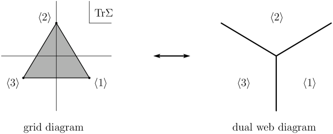
Fig. 1: The 3-pronged junction in the Abelian gauge theory. The left figure shows the grid diagram and the right shows its dual web diagram in the real spacial ($x^{1}$-$x^{2}$) plane.

One can easily read physical informations about domain walls and junctions from the grid diagram: The tension of the domain wall is proportional to the length of the corresponding edge of the grid diagram while the junction charge is to the area of the triangle. We have found previously that the topological charge of the Abelian junction gives a negative contribution to the energy of the configuration which can be interpreted as a binding energy of walls. We show the energy density of the Abelian junction in Fig.(2).

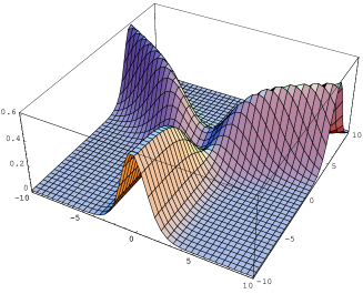
Fig. 2: The binding energy at the junction point: The energy density is numerically evaluated for the moduli matrix $H_{0}e^{\vec{m}\cdot\vec{x}}=\left(e^{x^{2}},\,e^{\sqrt{3}x^{1}/2-x^{2}/2},\,e^{-\sqrt{3}x^{1}/2-x^{2}/2}\right)$, gauge coupling $g=1$ and FI parameter $c=1$. The hole of the energy density at the junction point can be regarded as binding energy of the three walls.

One should note that the three vacua $\langle 1\rangle$, $\langle 2\rangle$ and $\langle 3\rangle$ are ordered counterclockwisely. On the other hand, non-Abelian junction appears in the case of $U(2)$ gauge theory ($N_{\rm C}=2$) and $N_{\rm F}=3$ with the same masses for hypermultiplets as in the above abelian theory. Then there appear the three vacua $\langle 12\rangle$, $\langle 23\rangle$and $\langle 31\rangle$ in the grid diagram which is congruent to the grid diagram of the Abelian case in Fig.1 : These two grid diagrams coincide when one of them is rotated by the angle $\pi$. Therefore tension of domain walls also coincides. However, the orientation for the non-Abelian junction is opposite to the Abelian junction, namely it is clockwise. This feature makes the $Y$-charge of the non-Abelian junction to contribute positively to the energy with the same magnitude. At the non-Abelian junction points an interesting system which is called the Hitchin system is realized. This positive $Y$-charge has been understood as the Hitchin charge of the Hitchin system [16].

In order to extract concrete informations from the moduli matrix $H_{0}$, it is useful to define the weight ${\cal W}^{\left<A_{r}\right>}$ of the vacuum $\left<A_{r}\right>=\left<A_{1}A_{2}\cdots A_{N_{\rm C}}\right>$ by

$${\cal W}^{\left<A_{r}\right>}(x^{1},x^{2})\equiv\sum_{r=1}^{N_{\rm C}}\left(m_{A_{r}}x^{1}+n_{A_{r}}x^{2}\right)+a^{\left<A_{r}\right>}.$$ (2.14)

Here we defined $a^{\left<A_{r}\right>}$ as a real part of $\log\det H_{0}^{\left<A_{r}\right>}=a^{\left<A_{r}\right>}+ib^{\left<A_{r}\right>}$, where $H_{0}^{\left<A_{r}\right>}$ is $N_{\rm C}\times N_{\rm C}$ minor matrix whose elements are given by $\left(H_{0}^{\left<A_{r}\right>}\right)^{s}{}_{t}=\left(H_{0}\right)^{s}{}_{A_{t}}$. Then $\Omega_{0}$ is given by

$$\det\Omega_{0}\equiv\det\left(\frac{1}{c}H_{0}e^{2(M_{1}x^{1}+M_{2}x^{2})}H_{0}^{\dagger}\right)=\log\left(\sum_{\langle A_{r}\rangle}e^{2{\cal W}^{\langle A_{r}\rangle}}\right).$$ (2.15)

Since the solution of the master equation $\Omega$ is well-approximated by $\Omega_{0}$ near vacuum regions, we can use the weight of the vacuum ${\cal W}^{\langle A_{r}\rangle}$ to estimate the regions where the vacuum $\langle A_{r}\rangle$ is dominant. Therefore, position of the domain wall which divides two vacua $\left<A_{r}\right>$ and $\left<B_{r}\right>$ (all the other weights are much smaller than these two) can be estimated from the condition of equating the weights of the vacua ${\cal W}^{\left<A_{r}\right>}\simeq{\cal W}^{\left<B_{r}\right>}$:

$$\sum_{r=1}^{N_{\rm C}}\left(m_{A_{r}}-m_{B_{r}}\right)x^{1}+\sum_{r=1}^{N_{\rm C}}\left(n_{A_{r}}-n_{B_{r}}\right)x^{2}+a^{\left<A_{r}\right>}-a^{\left<B_{r}\right>}\simeq 0.$$ (2.16)

Hence the parameter $a^{\left<A_{r}\right>}-a^{\left<B_{r}\right>}$ in the moduli matrix determines the position of the domain wall. Furthermore, one can see the angle of the domain wall is determined by the mass difference between the two vacua. Notice that the domain wall line (2.16) is perpendicular to the corresponding edge of the grid diagram, see Fig.1. So the grid diagram gives us information of the angle of domain wall in addition to the tension. A junction point at which three of domain walls get together can also be estimated by the condition of equating the weights of these three related vacua as ${\cal W}^{\left<A_{r}\right>}\simeq{\cal W}^{\left<B_{r}\right>}\simeq{\cal W}^{\left<C_{r}\right>}$.

3 Effective Actions on Networks/Webs of Walls

3.1 General Form of the Effective Action

Let us construct an effective theory on the world-volume of the networks/webs of walls. Zero modes on the background BPS solutions which are the lightest modes will play a main role in the effective theory while all the massive modes will be ignored in the following. Normalizable zero modes can be promoted to fields on the world-volume of the soliton background from mere parameters, with the assumption of weak dependence of the world-volume coordinates (slow move approximation à la Manton [18]). However, one should note that webs of walls contain nonnormalizable zero modes which cannot be promoted to effective fields and should be regarded as “couplings” of effective fields that are specified by boundary conditions[15, 16]. In the case of webs of walls, all the moduli parameters $\phi^{i}$ are contained in the moduli matrix $H_{0}(\phi^{i})$. So we promote normalizable modes to fields on the world-volume coordinates $x^{\mu}~{}~{}(\mu=0,3)$

$$H_{0}\bigl{(}\phi^{i}\bigr{)}\rightarrow H_{0}\bigl{(}\phi^{i}(x^{\mu})\bigr{)}.$$ (3.1)

Now we introduce “the slow-movement order parameter” $\lambda$, which is assumed to be much smaller than the other typical mass scales in the problem. There are two characteristic mass scales: one is mass difference $|\Delta m|$ of hypermultiplets, and the other is $g\sqrt{c}$ in front of the master equation. Therefore, we assume that

$$\lambda\ll\text{min}(|\Delta m|,g\sqrt{c}).$$ (3.2)

The non-vanishing fields in the 1/4 BPS background have contributions independent of $\lambda$, namely we assume that

$$H^{1}=\mathcal{O}(1),\quad W_{\alpha}=\mathcal{O}(1),\quad\Sigma_{\alpha}=\mathcal{O}(1).$$ (3.3)

The derivatives of these fields with respect to the world-volume coordinates are assumed to be of order $\lambda$ expressing the weak dependence on the world-volume coordinates. The vanishing fields in the background can now have non-vanishing values, induced by the fluctuations of the moduli fields of order $\lambda$. Therefore, we assume that

$$\partial_{\mu}=\mathcal{O}(\lambda),\quad W_{\mu}=\mathcal{O}(\lambda),\quad H^{2}=\mathcal{O}(\lambda).$$ (3.4)

Then the covariant derivative $\mathcal{D}_{\mu}={\cal O}(\lambda)$ has consistent $\lambda$ dependence.

If we expand the full equations of motion of the Lagrangian (2.1) in powers of $\lambda$, then we find that the $\mathcal{O}(1)$ equations are automatically satisfied due to the BPS equations. The next leading order $\mathcal{O}(\lambda)$ equation is the equation for $W_{\mu}$ including the Gauss law

$$0=-\frac{2}{g^{2}}\mathcal{D}_{\alpha}F_{\alpha\mu}+\frac{2i}{g^{2}}(\Sigma_{\alpha}\mathcal{D}_{\mu}\Sigma_{\alpha}-\mathcal{D}_{\mu}\Sigma_{\alpha}\Sigma_{\alpha})+i(H^{1}\mathcal{D}_{\mu}H^{1{\dagger}}-\mathcal{D}_{\mu}H^{1}H^{1{\dagger}}).$$ (3.5)

In order to obtain the effective action of order $\lambda^{2}$ on webs of walls, we have to solve this equation and determine the configuration of $W_{\mu}$.

Eq. (3.5) contains the derivatives of the world-volume coordinates $x^{\mu}~{}(\mu=0,3)$ on wall webs. As a consequence of Eq.(3.1), the moduli matrix $H_{0}(\phi^{i})$ depends on the world-volume coordinates $x^{\mu}$ through the moduli fields $\phi^{i}(x^{\mu})$. Note that for the fields which depend on $x^{\mu}$ only through the moduli fields, the derivatives with respect to the world-volume coordinates satisfy

$$\partial_{\mu}=\delta_{\mu}+\delta_{\mu}^{\dagger},$$ (3.6)

where we have defined the differential operators $\delta_{\mu}$ and $\delta_{\mu}^{\dagger}$ by

$$\delta_{\mu}\equiv\sum_{i}\partial_{\mu}\phi^{i}\frac{\delta}{\delta\phi^{i}},\quad\delta_{\mu}^{\dagger}\equiv\sum_{i}\partial_{\mu}\phi^{i\ast}\frac{\delta}{\delta\phi^{i\ast}},$$ (3.7)

respectively. Using these operators, the $\mathcal{O}(\lambda)$ equation of motion Eq.(3.5) can be solved, to yield

$$W_{\mu}=i(\delta_{\mu}S^{\dagger}S^{{\dagger}-1}-S^{-1}\delta_{\mu}^{\dagger}S).$$ (3.8)

The remaining work is to substitute these solutions into the fundamental Lagrangian (2.1) and to integrate over the codimensional coordinates $x^{1}$ and $x^{2}$. Since we are interested in the leading nontrivial part in powers of $\lambda$, we retain the terms up to $\mathcal{O}(\lambda^{2})$. We ignore a total derivative term which does not contribute to the effective Lagrangian, and obtain the effective Lagrangian of order ${\cal O}(\lambda^{2})$ as

$$\mathcal{L}^{eff} = \delta_{\mu}\delta^{\mu{\dagger}}K(\phi,\phi^{*})=K_{ij^{*}}(\phi,\phi^{*})\partial^{\mu}\phi^{i}\partial_{\mu}\phi^{j*},$$ (3.9)

$$K(\phi,\phi^{*}) = K_{w}(\phi,\phi^{*})+K_{g}(\phi,\phi^{*})$$ (3.10)

$$K_{w}(\phi,\phi^{*}) \equiv \int d^{2}x\,c\,\text{log det}\Omega,$$ (3.11)

$$K_{g}(\phi,\phi^{*}) \equiv \int d^{2}x\,\frac{1}{2g^{2}}\text{Tr}(\Omega^{-1}\partial_{\alpha}\Omega)^{2}.$$ (3.12)

From the above expression, we can see that the metric $K_{ij^{*}}$ on the moduli space is a Kähler metric whose Kähler potential is given by Eq. (3.10). We observe that the above formula is valid for the effective Lagrangian on the domain wall, if we restrict ourselves to single codimension, for instance $\alpha=1$ and integrate over $x^{1}$ alone when the wall is perpendicular to the $x^{1}$ axis. Note that the integral in Eqs. (3.11) and (3.12) for the Kähler potential has an infrared divergence ($x^{1},x^{2}\to\infty$). This comes from the fact that we have only constituent walls asymptotically ($x^{1},x^{2}\to\infty$). Since we have not promoted the nonnormalizable zero modes associated to the constituent walls and have fixed them by boundary conditions, these apparent contributions from asymptotic infinity to the Kähler potential can actually be eliminated by a Kähler transformation. Namely the infrared divergence can be removed by subtracting, from the integrand of Eqs. (3.11) and (3.12), some functions which are holomorphic or anti-holomorphic with respect to the effective fields.

We eventually got a Kähler geometry as a target space of a nonlinear sigma model on the moduli space: we did not expect Kähler geometry for effective action because it is $d=2$, ${\cal N}=(2,0)$ supersymmetric nonlinear sigma model [15, 46] whose geometry does not have to be Kähler in general [53, 54].

3.2 Single Triangle Loop

Let us first consider the effective action on a single triangle loop of walls. Here we will briefly review the construction of single triangle loop. In order to obtain a single triangle loop, we need at least four vacua. Here we consider the model with $N_{\rm C}=1$, $N_{\rm F}=4$ and masses

$$M\equiv M_{1}+iM_{2}=\text{diag}(m_{1}+in_{1},m_{2}+in_{2},m_{3}+in_{3},m_{4}+in_{4}).$$ (3.13)

The model with $N_{\rm C}=3$, $N_{\rm F}=4$ will be discussed in Sec. 4.5. In the $A$-th vacuum $\langle A\rangle$, the adjoint scalar takes the following vacuum expectation value:

$$\langle\Sigma\rangle_{\langle A\rangle}\equiv\langle\Sigma_{1}+i\Sigma_{2}\rangle_{\langle A\rangle}=m_{A}+in_{A}.$$ (3.14)

The moduli matrix which determines the configuration of walls is now a four-component row vector

$$H_{0}=\sqrt{c}(e^{a_{1}+ib_{1}},e^{a_{2}+ib_{2}},e^{a_{3}+ib_{3}},e^{a_{4}+ib_{4}}).$$ (3.15)

Now $\Omega_{0}$ is given by

$$\Omega_{0}\equiv\frac{1}{c}H_{0}e^{2(M_{1}x^{1}+M_{2}x^{2})}H_{0}^{\dagger}=\sum_{A=1}^{N_{\rm F}}e^{2\mathcal{W}^{\langle A\rangle}}.$$ (3.16)

Here we define the weight of vacuum $\langle A\rangle$ as

$$e^{2\mathcal{W}^{\langle A\rangle}}\equiv e^{2(m_{A}x^{1}+n_{A}x^{2}+a_{A})}.$$ (3.17)

In order to obtain a single triangle loop, we have to set mass parameters appropriately. Recall that the web diagram in the configuration space is dual of the grid diagram in the complex $\Sigma$ plane [15]. Therefore, a single triangle loop appears when the grid diagram consists of a triangle and one vacuum point is located inside the triangle (See Fig.(3)).

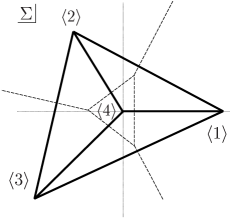
Fig. 3: Grid diagram and web diagram

For simplicity, we set the fourth complex mass parameter to zero and impose the following conditions:

$$\vec{m}_{1}\times\vec{m}_{2}>0,\quad\vec{m}_{2}\times\vec{m}_{3}>0,\quad\vec{m}_{3}\times\vec{m}_{1}>0,$$ (3.18)

where $\vec{m}_{i}\times\vec{m}_{j}\equiv m_{i}n_{j}-m_{j}n_{i}$.

Before constructing the effective action of the wall web, we have to know which mode is normalizable and which is not. In the present case, there exist three walls as external legs (we call them external walls): the wall interpolating $\langle 1\rangle$ and $\langle 2\rangle$, the one interpolating $\langle 2\rangle$ and $\langle 3\rangle$ and the one interpolating $\langle 3\rangle$ and $\langle 1\rangle$. These three walls have semi-infinite length. There also exist three internal walls as segments: the wall interpolating $\langle 1\rangle$ and $\langle 4\rangle$, the one interpolating $\langle 2\rangle$ and $\langle 4\rangle$ and the one interpolating $\langle 3\rangle$ and $\langle 4\rangle$. They constitute the single triangle loop. Zero modes which are related to the positions of the semi-infinite external walls, that is, zero modes which change the boundary condition at infinity are non-normalizable modes in the effective theory of the wall web. We should fix such non-normalizable modes. Therefore, the zero mode which is related to the size of the loop is the only possible normalizable mode.

In order to fix the three external walls, we fix three complex moduli parameters to 1 with leaving single complex parameter $\phi=e^{r+i\theta}$ which corresponds to the (dimensionless) size $r$ of the loop and the associated phase moduli $\theta$:

$$H_{0}=\sqrt{c}(1,1,1,\phi)~{}~{}~{}~{}\text{with}~{}~{}\phi=e^{r+i\theta}.$$ (3.19)

We promote this moduli parameter $\phi$ to a field on the world volume and construct the effective action for that. The configuration of the wall loop is given in Fig.4.

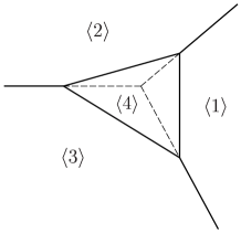
Fig. 4: Configuration of the wall loop

Next we have to solve the master equation (2.9) to explicitly construct the effective action. In order to do that, we take the strong coupling limit $g^{2}\rightarrow\infty$, in which the master equation can be solved algebraically as $\Omega=\Omega_{0}$. In the present case, $\Omega_{0}$ is given by

$$\Omega_{0}=e^{2\vec{m}_{1}\cdot\vec{x}}+e^{2\vec{m}_{2}\cdot\vec{x}}+e^{2\vec{m}_{3}\cdot\vec{x}}+|\phi|^{2}.$$ (3.20)

Substituting this solution to Eq.(3.10) and neglecting the second term ($g^{2}\to\infty$), we obtain the following Kähler potential

$$K=c\int d^{2}x\log\Omega_{0}=c\int d^{2}x\log(e^{2\vec{m}_{1}\cdot\vec{x}}+e^{2\vec{m}_{2}\cdot\vec{x}}+e^{2\vec{m}_{3}\cdot\vec{x}}+|\phi|^{2}).$$ (3.21)

Though this is apparently divergent, we can redefine the Kähler potential using the Kähler transformation to remove the moduli-independent divergence:

$$K_{w} \equiv c\,\int d^{2}x\left[\,\log\Omega_{0}-\log\,\tilde{\Omega}_{0}\,\right]=c\,\int d^{2}x\,\log\left(1+\frac{|\phi|^{2}}{\tilde{\Omega}_{0}}\right),$$ (3.22)

$$\tilde{\Omega}_{0} \equiv e^{2\vec{m}_{1}\cdot\vec{x}}+e^{2\vec{m}_{2}\cdot\vec{x}}+e^{2\vec{m}_{3}\cdot\vec{x}}.$$ (3.23)

We will show in the next section that this Kähler potential can be written as a sum of hypergeometric functions. We will obtain asymptotic metric in Sec. 4 by using another simple approach, which is valid for sufficiently large loop configuration $\phi\gg 1$. We will also calculate the asymptotic value of the second term $K_{g}$ in Eq. (3.10) in Sec. 4 without using explicit solutions. The meaning of the asymptotic metric will be clarified in Sec. 5.

3.3 Kähler Potential in terms of Hypergeometric Functions

Before trying to compute the Kähler potential, we first introduce the following notations:

$$\Delta_{[123]}=\vec{m}_{1}\times\vec{m}_{2}+\vec{m}_{2}\times\vec{m}_{3}+\vec{m}_{3}\times\vec{m}_{1},$$ (3.24)

$$\alpha_{1}\equiv\frac{(\vec{m}_{2}\times\vec{m}_{3})}{\Delta_{[123]}},\quad\alpha_{2}\equiv\frac{(\vec{m}_{3}\times\vec{m}_{1})}{\Delta_{[123]}},\quad\alpha_{3}\equiv\frac{(\vec{m}_{1}\times\vec{m}_{2})}{\Delta_{[123]}}.$$ (3.25)

Since the quantity $\tilde{\Omega}_{0}$ in Eq.(3.23) has the following minimum value

$$\log\tilde{\Omega}_{\rm min}=-\sum_{i=1}^{3}\alpha_{i}\log\alpha_{i}$$ (3.26)

as a function of $x^{1},x^{2}$, we can expand the integrand in powers of $\frac{|\phi|^{2}}{\tilde{\Omega}_{0}}$ as long as $|\phi|^{2}\leq\exp\left(-\sum\alpha_{i}\log\alpha_{i}\right)$

$$K_{w}=c\,\sum_{n=1}^{\infty}\frac{(-1)^{n+1}}{n}\int d^{2}x\frac{|\phi|^{2n}}{\tilde{\Omega}^{n}_{0}}.$$ (3.27)

Let us define the new variables of integration by

$$s_{1}=(\vec{m}_{1}-\vec{m}_{3})\cdot\vec{x},\hskip 14.22636pts_{2}=(\vec{m}_{2}-\vec{m}_{3})\cdot\vec{x}.$$ (3.28)

Then, for each $n$, we can integrate this in the following way:

$$\int^{\infty}_{-\infty}\frac{dx^{1}dx^{2}}{\tilde{\Omega}^{n}_{0}} = \frac{1}{\Delta_{[123]}}\int^{\infty}_{-\infty}ds_{1}ds_{2}\frac{e^{2n\alpha_{1}s_{1}}e^{2n\alpha_{2}s_{2}}}{(e^{2s_{1}}+e^{2s_{2}}+1)^{n}}$$ (3.29)

$$= \frac{1}{4\Delta_{[123]}}\int^{\infty}_{0}dudv\frac{u^{n\alpha_{1}-1}v^{n\alpha_{2}-1}}{\left(u+v+1\right)^{n}}\qquad(u=e^{2s_{1}},v=e^{2s_{2}})$$

$$= \frac{1}{4\Delta_{[123]}\Gamma(n)}\int^{\infty}_{0}dudvds\,u^{n\alpha_{1}-1}v^{n\alpha_{2}-1}s^{n-1}e^{-\left(u+v+1\right)s}$$

$$= \frac{1}{4\Delta_{[123]}}\frac{\Gamma(\alpha_{1}n)\Gamma(\alpha_{2}n)\Gamma(\alpha_{3}n)}{\Gamma(n)}.$$

Therefore we obtain the final form of the Kähler potential $K_{w}$ as

$$K_{w}=\frac{c}{4\Delta_{[123]}}\sum_{n=1}^{\infty}\frac{(-1)^{n+1}}{n}\frac{\Gamma(\alpha_{1}n)\Gamma(\alpha_{2}n)\Gamma(\alpha_{3}n)}{\Gamma(n)}|\phi|^{2n}.$$ (3.30)

We see that this series is convergent for $|\phi|^{2}\leq\exp\left(-\sum\alpha_{i}\log\alpha_{i}\right)$ and defines an analytic function of $|\phi|^{2}$ with a possible pole on the negative real axis. Therefore we know that there exists well-defined smooth function even for $|\phi|^{2}\geq\exp\left(-\sum\alpha_{i}\log\alpha_{i}\right)$. Moreover, this can be written as a sum of hypergeometric functions in cases where ${\alpha_{i}}$ are rational numbers. We can find out the behavior of this function outside the convergence region of the series by using the analytic continuation. In Appendix A, we give the detail of the analytic continuation to study the asymptotic behavior of a more general power series expression (A.2) including $K_{w}$ as a special case, and the expression in terms of hypergeometric functions. In the next section, we will show another simple approach to know the asymptotic metric for $|\phi|^{2}\gg 1$.

By using the expression Eq. (3.30), we can calculate the metric for $|\phi|^{2}\leq\exp\left(-\sum\alpha_{i}\log\alpha_{i}\right)$ as

$$K_{\phi\bar{\phi}}=\frac{\partial^{2}K_{w}}{\partial\phi\partial\bar{\phi}}=\frac{c}{4\Delta_{[123]}}\sum_{n=1}^{\infty}(-1)^{n+1}n\frac{\Gamma(\alpha_{1}n)\Gamma(\alpha_{2}n)\Gamma(\alpha_{3}n)}{\Gamma(n)}|\phi|^{2(n-1)}.$$ (3.31)

Since the loop of walls shrinks completely at $\phi=0$, one might think that the moduli space is singular at $\phi=0$. However, we can exactly calculate the scalar curvature from Eq. (3.31) at $\phi=0$ and find that it is finite:

$$R=\frac{16\Delta_{[123]}}{c}\frac{\Gamma(2\alpha_{1})\Gamma(2\alpha_{2})\Gamma(2\alpha_{3})}{\left(\Gamma(\alpha_{1})\Gamma(\alpha_{2})\Gamma(\alpha_{3})\right)^{2}}+\mathcal{O}(|\phi|^{2}).$$ (3.32)

Therefore, the moduli space of the single loop is non-singular at $\phi=0$.

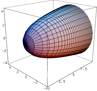
Fig. 5: The moduli space of single triangle loop embedded in $\mathbf{R}^{3}$: The moduli space has a $U(1)$ isometry which corresponds to the direction of the phase modulus. The other direction can be regarded as the direction of size modulus of the loop. The tip of the moduli space corresponds to the point $\phi=0$ where the loop shrinks completely.

Fig. 5 illustrates the moduli space of the single loop embedded into the three dimensional Euclidean space.

4 Large Size Behavior: Tropical Limit

4.1 Tropical Limit

To evaluate the asymptotic metric of the moduli space at large loop size, we note that $\log{\rm det}\Omega$ is well approximated by $\log{\rm det}\Omega_{0}$ apart from tiny finite regions near walls and junctions. By excluding these finite regions near walls and junctions, space is divided into a number of regions corresponding to various vacua. In each region, only the weight of a single vacuum is dominant in $\log{\rm det}\Omega_{0}$

$$\log\det\Omega_{0}=\log\left(\sum_{\langle A_{r}\rangle}e^{2{\cal W}^{\langle A_{r}\rangle}}\right)\to\underset{\langle A\rangle}{\rm max}\,\left(2{\cal W}^{\langle A\rangle}\right),$$ (4.1)

where the weight of the vacuum ${\cal W}^{\langle A\rangle}$ is defined in Eqs.(2.14) and (2.15). We call this procedure “tropical limit”. It will turn out that the tropical limit exactly extracts the leading contribution from the Kähler potential and the correction terms are strongly suppressed in sufficiently large loop configuration $|\phi|^{2}\gg 1$. Moreover, the tropical limit is applicable irrespective of the value of gauge coupling $g$.

As a concrete example, let us take the Abelian gauge theory with four flavors. The configuration of single triangle loop has three external walls and three internal walls, which divide the $x^{1}$-$x^{2}$ plane into four regions, $\langle 1\rangle$, $\langle 2\rangle$, $\langle 3\rangle$ and $\langle 4\rangle$ (See Fig. 4). In each region $\langle A\rangle,\,(A=1,2,3,4)$, the corresponding weight $e^{2{\cal W}^{\langle A\rangle}}$ is largest among four weights. In the present section, we will consider only the largest weight in each region and simply drop the other weights to roughly evaluate the Kähler potential. Namely, we consider the limit in which the logarithmic function becomes

$$\log\Omega_{0}=\log\left(e^{2{\cal W}^{\langle 1\rangle}}+e^{2{\cal W}^{\langle 2\rangle}}+e^{2{\cal W}^{\langle 3\rangle}}+e^{2{\cal W}^{\langle 4\rangle}}\right)\rightarrow\underset{1\leq A\leq 4}{\rm max}\,\left(2{\cal W}^{\langle A\rangle}\right)$$ (4.2)

4.2 Tropical Limit in 1/2 BPS Parallel Walls

Before considering the case of large $|\phi|^{2}$ of the loop of the walls, let us consider simpler example of two parallel walls and evaluate concretely an effective Kähler potential for a relative distance (and a relative phase) between two walls. This computation should serve as a warm-up exercise for the more complicated case of wall loops. The model for $N_{\rm C}=1$ and $N_{\rm F}=3$ with non-degenerate real masses $m_{A}(A=1,2,3)$ have three different vacua characterized by $\Sigma_{1}+i\Sigma_{2}=m_{1},m_{2},m_{3}\in{\bf R}$ and allows a BPS solution of double walls with two complex moduli parameters. We can take one of the two to be the center of mass position and the overall phase which are Nambu-Goldstone modes and normalizable in this case of parallel walls. Therefore we promote it to free particles in the effective action. Let us now concentrate to the other complex moduli $\phi=e^{r+i\theta}$. A real part $r$ can be interpreted as the relative distance if $|\phi|>1$, and it’s imaginary part $\theta$ gives the relative phase between two walls. A Kähler potential of an effective action for a chiral field $\phi$ in the strong coupling limit is obtained by performing the following integral [42],

$$K_{\rm wall}=c\,\int_{-\infty}^{\infty}dy\left\{\log\left(e^{2m\alpha_{1}y}+e^{-2m\alpha_{2}y}+|\phi|^{2}\right)-\log\left(e^{2m\alpha_{1}y}+e^{-2m\alpha_{2}y}\right)\right\}$$ (4.3)

where we denoted the mass parameters as $(m_{1},m_{2},m_{3})=(m\alpha_{1},\,0,\,-m\alpha_{2})$ with $m\equiv m_{1}-m_{3}$, $\alpha_{1}+\alpha_{2}=1$ and $0<\alpha_{1}<1$ without loss of generality. To perform the integration for large $r$, let us decompose the integral into four integrals with respect to intervals $I_{i},(i=1,\cdots,4)$

$$I_{1}\equiv\{y|e_{1}\geq e_{0}\geq e_{2}\}=\big{\{}y\big{|}my\geq\frac{r}{\alpha_{1}}\big{\}},$$

$$I_{2}\equiv\{y|e_{0}>e_{1}\geq e_{2}\}=\big{\{}y\big{|}\frac{r}{\alpha_{1}}>my\geq 0\big{\}},$$

$$I_{3}\equiv\{y|e_{0}\geq e_{2}>e_{1}\}=\big{\{}y\big{|}0>my\geq-\frac{r}{\alpha_{2}}\big{\}},$$

$$I_{4}\equiv\{y|e_{2}>e_{0}>e_{1}\}=\big{\{}y\big{|}my<-\frac{r}{\alpha_{2}}\big{\}},$$ (4.4)

with abbreviations $e_{1}=e^{2m\alpha_{1}y},e_{2}=e^{-2m\alpha_{2}y},e_{0}=e^{2r}$. Here, note that $\frac{r}{\alpha_{1}},-\frac{r}{\alpha_{2}}$ are (dimensionless) positions of walls and the center of mass position is chosen to vanish. The various informations are illustrated in Fig. 6.

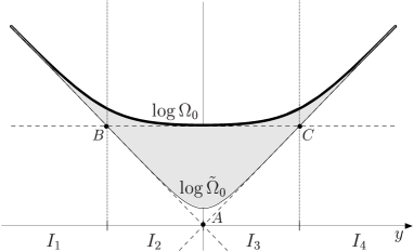
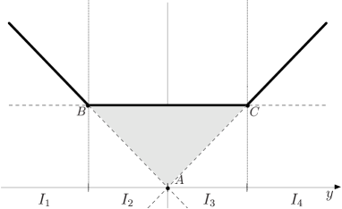
(a) Plot of $\log\Omega_{0}$ and $\log\tilde{\Omega}_{0}$	(b) Tropical limit of $\log\Omega_{0}$

Fig. 6: The Kähler potential is given by the area of the shaded region in (a). The area of the triangle $ABC$ (first term in Eq. (4.12)) gives the leading contribution to the Kähler potential for large $r$.

In the interval $I_{1}$, it is convenient to perform the integral by decomposing the integrand into

$$\log(e_{1}+e_{2}+e_{0})-\log(e_{1}+e_{2})$$ (4.5)

$$= \log\left(1+\frac{e_{0}}{e_{1}}\right)-\log\left(1+\frac{e_{2}}{e_{1}}\right)+\log\left(1+\frac{e_{2}}{e_{1}+e_{0}}\right),$$

so that logarithmic function can be expanded to infinite series as $\log(1+x)=\sum_{n=1}^{\infty}\frac{(-1)^{n-1}}{n}x^{n}$. Note that the term $\log e_{1}$ which gives divergent integral cancels out. In the interval $I_{2}$, we also take a decomposition of the integrand as

$$\left(\log e_{0}-\log e_{1}\right)+\log\left(1+\frac{e_{1}}{e_{0}}\right)-\log\left(1+\frac{e_{2}}{e_{1}}\right)+\log\left(1+\frac{e_{2}}{e_{1}+e_{0}}\right),$$ (4.6)

The first term gives leading terms of the integral as

$$\int_{I_{2}}dy\left(\log e_{0}-\log e_{1}\right)=\int_{\frac{r}{m\alpha_{1}}}^{0}dy\,\left(2r-2m\alpha_{1}y\right)=\frac{1}{m\alpha_{1}}r^{2},$$ (4.7)

and next leading terms are calculated as

$$\int_{I_{1}}dy\log\left(1+\frac{e_{0}}{e_{1}}\right) = \sum_{n=1}^{\infty}\frac{(-1)^{n-1}}{n}e^{2nr}\int_{\frac{r}{\alpha_{1}}}^{\infty}dy\,e^{-2n\alpha_{1}y}=\frac{1}{2m\alpha_{1}}\frac{\pi^{2}}{12},\qquad\quad$$ (4.8)

$$\int_{I_{2}}dy\log\left(1+\frac{e_{1}}{e_{0}}\right) = \frac{1}{2m\alpha_{1}}\left(\frac{\pi^{2}}{12}-\sum_{n=1}^{\infty}\frac{(-1)^{n-1}}{n^{2}}e^{-2nr}\right),$$ (4.9)

$$-\int_{I_{1}+I_{2}}dy\log\left(1+\frac{e_{2}}{e_{1}}\right) = -\frac{1}{2m}\frac{\pi^{2}}{12},$$ (4.10)

where we used an identity $\sum_{n=1}\frac{(-1)^{n-1}}{n^{2}}=\frac{1}{2}\zeta(2)=\frac{\pi^{2}}{12}$. We also find the integrals for the intervals $I_{3}$ and $I_{4}$ give the same contributions as $I_{2}$ and $I_{1}$, respectively, except for exchanging the parameters $\alpha_{1}$ and $\alpha_{2}$. There remain the last terms $\log(1+\frac{e_{2}}{e_{1}+e_{0}})$ in Eqs.(4.5) and (4.6). They should be integrated over $y$ in the region $I_{1}$ and $I_{2}$, respectively, and are evaluated in appendix B. The result can be combined with the last term (sum over $n$ of $e^{-2nr}$ terms) in Eq.(4.9) to give only contributions of order of $e^{-\frac{2}{\alpha_{1}}r}$. These correction terms are guaranteed to be finite by inequalities

$$0<\int_{I_{1},I_{2}}dy\log\left(1+\frac{e_{2}}{e_{1}+e_{0}}\right)<\int_{I_{1},I_{2}}dy\log\left(1+\frac{e_{2}}{e_{1}}\right)={\rm constant}.$$ (4.11)

Thus we obtain

$$K_{\rm wall}=\frac{c}{\alpha_{1}\alpha_{2}m}r^{2}+\frac{c}{2m}\left(\frac{1}{\alpha_{1}}+\frac{1}{\alpha_{2}}-1\right)\frac{\pi^{2}}{6}+{\cal O}(e^{-\frac{2}{\alpha_{1}}r},e^{-\frac{2}{\alpha_{2}}r}).$$ (4.12)

It is remarkable that there are no terms proportional to the length $r$ of the relative distance of walls in the Kähler potential. This is because the deviation from the tropical limit is localized in finite regions around points $A,B,C$ and does not increase as the distance $r$ between $B$ and $C$ increases. This feature holds irrespective of values of gauge coupling $g$. Therefore our approximation with the tropical limit as the leading term is applicable for any finite values of gauge coupling $g$. One should note that the constant contribution (the second term) in the right-hand side of Eq.(4.12) is a nontrivial physical constant, even though the term gives no contribution locally to the Kähler metric. For instance, if we fix the Kähler potential at $\phi=0$ ($r=-\infty$) to vanish, we can no longer eliminate the constant term by Kähler transformations.

4.3 Tropical Limit in Single Triangle Loop

Our starting point is Eq.(3.22) where the moduli-independent divergence has already been removed. As we mentioned before, we divide the integral region to four parts, $\langle 1\rangle,\langle 2\rangle,\langle 3\rangle$ and $\langle 4\rangle$ and pick up only the largest weight in each region. In integrating the second term, we also divide the integral region to three parts, and pick up only single weight which is largest in each region.

To illustrate what we are doing clearly, let us show the division of the integration region in Fig.7.

Fig. 7: Division of the integral region

If we denote each weight $e^{2{\cal W}^{\langle A\rangle}}$ as $e_{A}$, the order of four weights is $e_{1}\geq e_{2}\geq e_{4}\geq e_{3}$ in the region $S_{1}$. The integrand in Eq.(3.22) can be rewritten as

$$\log (e_{1}+e_{2}+e_{3}+e_{4})-\log(e_{1}+e_{2}+e_{3})$$

$$=\log e_{1}+\log\left(1+\frac{e_{2}}{e_{1}}\right)+\log\left(1+\frac{e_{4}}{e_{1}+e_{2}}\right)+\log\left(1+\frac{e_{3}}{e_{1}+e_{2}+e_{4}}\right)$$

$$~{}~{}-\log e_{1}-\log\left(1+\frac{e_{2}}{e_{1}}\right)-\log\left(1+\frac{e_{3}}{e_{1}+e_{2}}\right)$$

$$=\log\left(1+\frac{e_{4}}{e_{1}+e_{2}}\right)-\log\left(1+\frac{e_{3}}{e_{1}+e_{2}}\right)+\log\left(1+\frac{e_{3}}{e_{1}+e_{2}+e_{4}}\right)$$ (4.13)

in the region $S_{1}$. The leading contribution, $\log e_{1}$, cancels here. Similar cancellation occurs in $S_{2},S_{3}$ and $S_{4}$. However, in the region $S_{5}$, the order of four weights is $e_{4}\geq e_{1}\geq e_{2}\geq e_{3}$ and the integrand can be rewritten as

$$\log (e_{1}+e_{2}+e_{3}+e_{4})-\log(e_{1}+e_{2}+e_{3})$$

$$=\log e_{4}+\log\left(1+\frac{e_{1}}{e_{4}}\right)+\log\left(1+\frac{e_{2}}{e_{4}+e_{1}}\right)+\log\left(1+\frac{e_{3}}{e_{4}+e_{1}+e_{2}}\right)$$

$$~{}~{}-\log e_{1}-\log\left(1+\frac{e_{2}}{e_{1}}\right)-\log\left(1+\frac{e_{3}}{e_{1}+e_{2}}\right).$$ (4.14)

The tropical limit yields non-zero value $\log e_{4}-\log e_{1}$ for the leading contribution in the region $S_{5}$. Similarly, in the region $S_{6}$, the leading contribution is $\log e_{4}-\log e_{1}$. Contributions from the other regions can be obtained by rotating the label $i(i=1,2,3)$ cyclically.

Note that the leading contribution can be computed as the volume of the tetrahedron. This can be easily seen from Fig.8.

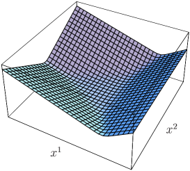
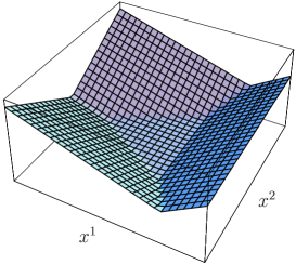
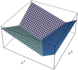
(a)	(b)	(c)

Fig. 8: (a) plot of $\log\Omega_{0},$ (b)  tropical limit of $\log\Omega_{0}$, (c)  tropical limit of $\log\tilde{\Omega}_{0}$

$$K_{w}^{trop} =c\cdot\text{volume of the tetrahedron}$$

$$=\frac{c}{24\Delta_{[123]}}\frac{1}{\alpha_{1}\alpha_{2}\alpha_{3}}(\log|\phi|^{2})^{3}.$$ (4.15)

It is important to note that there are no subleading terms of the form $(\log|\phi|^{2})^{2}$, as shown in Eq.(A.13) in Appendix A.2. Since deviations from the tropical limit are localized in finite regions around walls and junctions, there are contributions proportional to the wall length $\log|\phi|^{2}$ and constant contributions associated with junctions. Therefore there is no contribution proportional to the area $(\log|\phi|^{2})^{2}$ in Fig.8. This tropical approximation should be valid for finite values of coupling constant $g$.

The variation of this potential yields the following simple asymptotic metric:

$$ds_{w}^{2} =\frac{c}{\Delta_{[123]}}\frac{r}{\alpha_{1}\alpha_{2}\alpha_{3}}(dr^{2}+d\theta^{2})$$

$$=\frac{c}{2\Delta_{[123]}}\frac{1}{\alpha_{1}\alpha_{2}\alpha_{3}}\left(dR^{2}+\left(\frac{3}{2}R\right)^{\frac{2}{3}}d\theta^{2}\right),$$ (4.16)

where subleading contributions should be suppressed by powers of $1/|\phi|\sim e^{-r}$, as illustrated in Appendix B for the case of walls. In Fig.9, the numerically evaluated metric $g_{rr}$ of moduli space is compared to the asymptotic metric (4.16) evaluated at $r\to\infty$ with $g\to\infty$.

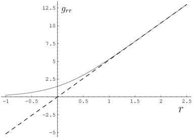
Fig. 9: Metric of moduli space (solid line) $g_{rr}$ and asymptotic metric (dashed line).                       We have chosen $\vec{m}_{1}=(1,~{}0),~{}\vec{m}_{2}=(-1/2,~{}\sqrt{3}/2),~{}\vec{m}_{3}=(-1/2,~{}-\sqrt{3}/2)$, and $c=1,\,g\to\infty$.

4.4 Tropical limit at Finite Couplings

In the previous subsection, we have evaluated the asymptotic behavior for large values of moduli and obtained the Kähler potential in the tropical limit. This tropical limit contains only informations of vacua and does not require the detailed informations on the internal structure of walls and/or junctions. The tropical limit should be applicable to a solution obtained in arbitrary coupling constant. In the following we use vacuum expectation values to evaluate Eq. (3.12).

The key point is that from the second equation of Eq.(2.6) $\Sigma_{\alpha}$ can be written as

$$\Sigma_{\alpha}=\frac{1}{2}S^{-1}\partial_{\alpha}\Omega S^{{\dagger}-1}.$$ (4.17)

Using this relation, the integrand in Eq.(3.12) can be rewritten as

$$\frac{1}{2g^{2}}{\rm Tr}\bigl{[}(\Omega^{-1}\partial_{\alpha}\Omega)^{2}\bigr{]}=\frac{2}{g^{2}}{\rm Tr}~{}\Sigma_{\alpha}^{2}.$$ (4.18)

Note that in the vacuum $\langle A\rangle$, $\Sigma_{\alpha}^{2}$ takes the value

$$\langle\Sigma_{\alpha}^{2}\rangle_{\langle A\rangle}=m_{A}^{2}+n_{A}^{2}.$$ (4.19)

See Eq.(3.14). Therefore, the tropical limit yields

$$\frac{1}{2g^{2}}{\rm Tr}\bigl{[}(\Omega^{-1}\partial_{\alpha}\Omega)^{2}\bigr{]}\rightarrow\frac{2}{g^{2}}|\vec{m}_{A}|^{2}$$ (4.20)

in region $\langle A\rangle$. Note that this is constant and does not depend on the coordinates $x^{1}$ and $x^{2}$.

Before trying to compute, we remove moduli-independent divergence by using the Kähler transformation as before

$$K_{g}\equiv\int d^{2}x\frac{1}{2g^{2}}{\rm Tr}\bigl{[}(\Omega^{-1}\partial_{\alpha}\Omega)^{2}-(\tilde{\Omega}^{-1}\partial_{\alpha}\tilde{\Omega})^{2}\bigr{]}.$$ (4.21)

Here $\tilde{\Omega}$ means $\tilde{\Omega}=\Omega(|\phi|=0)$. In the tropical limit, the external vacuum regions $\langle A\rangle,(A=1,2,3)$ give vanishing contributions, whereas the vacuum region $\langle 4\rangle$ inside the loop gives a non-zero contribution, as before. See Fig. 10 (a) and (b).

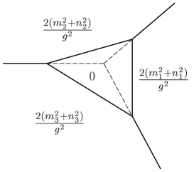
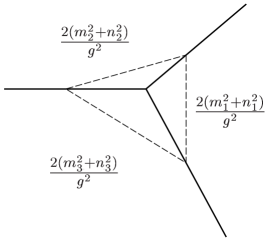
(a)	(b)	(c)

Fig. 10: (a) tropical limit of $\frac{1}{2g^{2}}\text{Tr}\bigl{[}(\Omega^{-1}\partial_{\alpha}\Omega)^{2}\bigr{]},$ (b) tropical limit of $\frac{1}{2g^{2}}\text{Tr}\bigl{[}(\tilde{\Omega}^{-1}\partial_{\alpha}\tilde{\Omega})^{2}\bigr{]}$, (c) division of area of the loop

Therefore, the tropical limit yields

$$K_{g}^{trop} =-\frac{2}{g^{2}}|\vec{m}_{1}|^{2}A_{1}-\frac{2}{g^{2}}|\vec{m}_{2}|^{2}A_{2}-\frac{2}{g^{2}}|\vec{m}_{3}|^{2}A_{3}$$

$$=-\frac{1}{4g^{2}\Delta_{[123]}}\left(\frac{|\vec{m}_{12}|^{2}}{\alpha_{3}}+\frac{|\vec{m}_{23}|^{2}}{\alpha_{1}}+\frac{|\vec{m}_{31}|^{2}}{\alpha_{2}}\right)(\log|\phi|^{2})^{2}.$$ (4.22)

Here $A_{i}$ is the area of the loop, which is given in Fig.10(c) and $\vec{m}_{AB}=\vec{m}_{A}-\vec{m}_{B}$. The variation of this potential leads to the following contribution to the metric.

$$ds_{g}^{2}=-\frac{1}{g^{2}\Delta_{[123]}}\left(\frac{|\vec{m}_{12}|^{2}}{\alpha_{3}}+\frac{|\vec{m}_{23}|^{2}}{\alpha_{1}}+\frac{|\vec{m}_{31}|^{2}}{\alpha_{2}}\right)(dr^{2}+d\theta^{2}).$$ (4.23)

Let us combine the contributions $ds_{w}^{2}$ in Eq.(4.16) and $ds_{g}^{2}$ in Eq.(4.23) together to give the total Kähler metric in the asymptotic region obtained by the tropical limit

$$ds^{2}= \frac{c}{\Delta_{[123]}}\left[\frac{r}{\alpha_{1}\alpha_{2}\alpha_{3}}-\frac{1}{g^{2}c}\left(\frac{|\vec{m}_{12}|^{2}}{\alpha_{3}}+\frac{|\vec{m}_{23}|^{2}}{\alpha_{1}}+\frac{|\vec{m}_{31}|^{2}}{\alpha_{2}}\right)\right](dr^{2}+d\theta^{2}).$$ (4.24)

Since the tropical limit does not require the details of the solution and contains only the information of vacua, this result should be applicable to solutions for the general cases with arbitrary masses and arbitrary coupling $g$. Using the explicit solution in the strong coupling limit $\Omega=\Omega_{0}$, we will estimate the correction terms and show in Appendix B that the corrections to the Kähler metric of the tropical limit should be suppressed exponentially for large $r$.

4.5 Tropical Limit in Non-Abelian Single Triangle Loop

In this section, let us consider the non-Abelian gauge theory with $N_{\rm C}=3$, $N_{\rm F}=4$. This model has also four vacua, $\langle A_{r}\rangle=\langle 123\rangle,\langle 124\rangle,\langle 134\rangle$ and $\langle 234\rangle$. In order to compare with the Abelian model, we choose the same mass parameters as that of the Abelian gauge theory with $N_{\rm C}=1$, $N_{\rm F}=4$ in Sec. 3.2.

Although the moduli matrix $H_{0}$ is $3\times 4$ in this case, we extract $3\times 3$ matrix $H_{0}^{\langle A_{r}\rangle}$ defined by $(H_{0}^{\langle A_{r}\rangle})^{s}_{~{}t}=(H_{0})^{s}_{~{}A_{t}}$. Then we choose moduli parameters as

$$\det H_{0}^{\langle 234\rangle}=\det H_{0}^{\langle 134\rangle}=\det H_{0}^{\langle 124\rangle}=1,\hskip 14.22636pt\det H_{0}^{\langle 123\rangle}=\phi=e^{r+i\theta}.$$ (4.25)

There is an exact correspondence between vacua of the $U(N_{\rm C})$ gauge theory with $N_{\rm F}$ flavors to those of the $U(N_{\rm F}-N_{\rm C})$ gauge theory with $N_{\rm F}$ flavors[56]. The moduli space point (4.25) in the $U(3)$ gauge theory and the moduli space point (3.19) in the $U(1)$ gauge theory give different ${\rm det}\Omega$, which reduces to the same ${\rm det}\Omega_{0}$ near vacuum regions because of this correspondence. In the tropical limit, we evaluate $\Omega$ by replacing it with $\Omega_{0}$ dominated by the single dominant vacuum weight. We only need informations on vacuum regions. Therefore, the asymptotic metric (4.16) corresponding to the first term in Eq.(3.10) is also valid in the $U(3)$ gauge theory.

The difference appears in the second term in Eq.(3.10). From Eq.(4.18), the tropical limit leads to

$$\frac{1}{2g^{2}}{\rm Tr}\bigl{[}(\Omega^{-1}\partial_{\alpha}\Omega)^{2}\bigr{]}\rightarrow\frac{2}{g^{2}}(|\vec{m}_{A}|^{2}+|\vec{m}_{B}|^{2}+|\vec{m}_{C}|^{2})$$ (4.26)

in the vacuum $\langle ABC\rangle$ of the $U(3)$ gauge theory corresponding to the $\langle D\rangle$ of the $U(1)$ gauge theory. If we remove the moduli-independent divergence as before, non-zero contribution comes only from the vacuum $\langle 123\rangle$. Therefore, this yields the same form of the asymptotic metric but its sign is flipped

$$ds_{g}^{2}=\frac{1}{2g^{2}\Delta_{[123]}}\Bigl{(}\frac{|\vec{m}_{12}|^{2}}{\alpha_{3}}+\frac{|\vec{m}_{23}|^{2}}{\alpha_{1}}+\frac{|\vec{m}_{31}|^{2}}{\alpha_{2}}\Bigr{)}(dr^{2}+d\theta^{2}).$$ (4.27)

This result is quite intriguing. The meaning of the plus sign will be clarified in section 5.

5 Understanding of the Asymptotic Metric

In this section we clarify the physical meaning of the asymptotic metric.

5.1 Kinetic Energy of Walls

We are now considering the dynamics of a system which consists of three internal walls and has two kinematic variables $r$ and $\theta$. (Three external walls have been fixed by boundary conditions. ) There is no potential energy among the three walls due to the BPS nature of this system. Therefore, the effective Lagrangian of single triangle loop would be simply given by the kinetic energy of internal walls.

The metric (4.16) expresses this kinetic energy of walls. Let us confirm this statement.
First of all, lengths of internal walls are given by

$$\langle 1\rangle\langle 4\rangle~{}\text{wall}\quad l^{(1,4)}=\frac{|{\vec{m}_{1}}|}{\Delta_{[123]}}\frac{1}{\alpha_{3}\alpha_{2}}r,$$

$$\langle 2\rangle\langle 4\rangle~{}\text{wall}\quad l^{(2,4)}=\frac{|{\vec{m}_{2}}|}{\Delta_{[123]}}\frac{1}{\alpha_{1}\alpha_{3}}r,$$

$$\langle 3\rangle\langle 4\rangle~{}\text{wall}\quad l^{(3,4)}=\frac{|{\vec{m}_{3}}|}{\Delta_{[123]}}\frac{1}{\alpha_{2}\alpha_{1}}r.$$ (5.1)

Tensions of internal walls are

$$\langle 1\rangle\langle 4\rangle~{}\text{wall}\quad T^{(1,4)}=c|\vec{m}_{1}|,$$

$$\langle 2\rangle\langle 4\rangle~{}\text{wall}\quad T^{(2,4)}=c|\vec{m}_{2}|,$$

$$\langle 3\rangle\langle 4\rangle~{}\text{wall}\quad T^{(3,4)}=c|\vec{m}_{3}|.$$ (5.2)

Next we have to know how the internal walls move when the variable $r$ changes. We denote the distances between the origin and internal walls as $l_{0}^{(A4)},(A=1,2,3)$. These are given by

$$\langle 1\rangle\langle 4\rangle~{}\text{wall}\quad l_{0}^{(1,4)}=\frac{r}{|\vec{m}_{1}|},$$

$$\langle 2\rangle\langle 4\rangle~{}\text{wall}\quad l_{0}^{(2,4)}=\frac{r}{|\vec{m}_{2}|},$$

$$\langle 3\rangle\langle 4\rangle~{}\text{wall}\quad l_{0}^{(3,4)}=\frac{r}{|\vec{m}_{3}|}.$$ (5.3)

Therefore, the total kinetic energy of internal walls is

$$T= \sum_{A=1}^{3}\frac{1}{2}T^{(A,4)}l^{(A,4)}\left(\frac{d}{dt}l^{(A,4)}_{0}\right)^{2}=\frac{c}{2\Delta_{[123]}}\frac{r}{\alpha_{1}\alpha_{2}\alpha_{3}}\left(\frac{dr}{dt}\right)^{2}.$$ (5.4)

We observe that the moduli space metric at $g^{2}\to\infty$ in Eq.(4.23) agrees with this result, since the total kinetic energy should be expressed in terms of the metric as

$$T=\frac{1}{2}\left(\frac{ds_{w}}{dt}\right)^{2}.$$ (5.5)

5.2 Kinetic Energy of Junction Charges

In the above, we considered only the kinetic energy of internal walls. However, the mass of a wall web actually consists of energies of walls (tension $T_{w}$ times the length of the walls) and a contribution from the junction charge $Y$. The $Y$ contributes negatively to the energy in the $U(1)$ gauge theory and is interpreted as the binding energy of the three walls. If $r$ changes to $r+dr$, the junction points also moves slightly, which accompanies the movement of junction charges at the junction points. Therefore, it is natural to expect that the metric (4.23) expresses the “kinetic energy” of junction charges, which is negative because of the negative “mass” of the junction. Junction charges are given by

$$\langle 124\rangle~{}\text{junction}\quad Y^{124}=-\frac{\Delta_{[123]}}{g^{2}}\alpha_{3},$$

$$\langle 234\rangle~{}\text{junction}\quad Y^{234}=-\frac{\Delta_{[123]}}{g^{2}}\alpha_{1},$$

$$\langle 314\rangle~{}\text{junction}\quad Y^{314}=-\frac{\Delta_{[123]}}{g^{2}}\alpha_{2}.$$ (5.6)

Distances between the origin and the junctions are

$$\langle 124\rangle~{}\text{junction}\quad l^{124}=\frac{|\vec{m}_{12}|}{\Delta_{[123]}\alpha_{3}}r,$$

$$\langle 234\rangle~{}\text{junction}\quad l^{234}=\frac{|\vec{m}_{23}|}{\Delta_{[123]}\alpha_{1}}r,$$

$$\langle 314\rangle~{}\text{junction}\quad l^{314}=\frac{|\vec{m}_{31}|}{\Delta_{[123]}\alpha_{2}}r.$$ (5.7)

Using these, we obtain the kinetic energy of junction charges

$$T = T^{124}+T^{234}+T^{314}$$ (5.8)

$$= -\frac{1}{2g^{2}\Delta_{[123]}}\left(\frac{|\vec{m}_{12}|^{2}}{\alpha_{3}}+\frac{|\vec{m}_{23}|^{2}}{\alpha_{1}}+\frac{|\vec{m}_{31}|^{2}}{\alpha_{2}}\right)\left(\frac{dr}{dt}\right)^{2}.$$

This agrees with the result in Eq.(4.23) of the Abelian gauge theory.

This interpretation naturally explains the sign difference between Eq.(4.23) and Eq.(4.27). In the non-Abelian junction, junction charge gives a positive contribution to energy of a wall web in contrast to the Abelian junction. This can be interpreted as the $Y$-charge of the Hitchin system. For the details about these issues, see [16].

The non-Abelian junction charges have the same magnitude as the Abelian junction charges (5.6) but its sign is reversed.

$$\langle 234\rangle\langle 134\rangle\langle 123\rangle\quad\text{junction}\quad Y^{124}=\frac{\Delta_{[123]}}{g^{2}}\alpha_{3},$$

$$\langle 134\rangle\langle 124\rangle\langle 123\rangle\quad\text{junction}\quad Y^{234}=\frac{\Delta_{[123]}}{g^{2}}\alpha_{1},$$

$$\langle 124\rangle\langle 234\rangle\langle 123\rangle\quad\text{junction}\quad Y^{124}=\frac{\Delta_{[123]}}{g^{2}}\alpha_{2}.$$ (5.9)

This explains the sign flip in the asymptotic metric of Eq.(4.27) compared to that of Eq.(4.23).

6 Conclusion and Discussion

We have constructed an effective theory of webs/networks of domain walls. The general form of the effective action Eq. (3.9) is written in terms of the Kähler potential given by Eq. (3.10), (3.11), (3.12). In the strong coupling limit $g^{2}\rightarrow\infty$, the Kähler potential for the single triangle loop can be written in the form of the power series as Eq. (3.30). The moduli space is smooth even at the point where the size of the loop shrinks to zero. The large size behavior of the Kähler potential can be calculated as Eq. (4.16) by using the tropical limit. In this limit we can also evaluate the contributions from the junction charges in the Abelian case Eq. (4.23) and in the non-Abelian case Eq. (4.27). These asymptotic metrics can be read from kinetic energy of the constituent walls of the loop and the junction charges.

Let us summarize possible future works. Since the metric of the moduli space of a single loop has been obtained, its dynamics can be discussed by the moduli space (Manton’s) approximation. We also should extend our work to multiple loops of domain walls. These aspects will be reported elsewhere [57].

The parallel domain walls have dyonic extension [45] if we introduce complex masses. In the case of domain wall webs, they admit dyonic extension if the triplet of masses is introduced [46]. In the case of supersymmetric field theory, this is possible in a $d=2+1$ theory which can be obtained by the Scherk-Schwarz dimensional reduction from the $d=3+1$ theory discussed in this paper. The effective action on webs becomes a classical mechanics (a $d=1$ nonlinear sigma model). Since it is known that a potential, which is proportional to a square of a Killing vector of a $U(1)$ isometry of the moduli space, is induced on the effective theory of dyons [58] or dyonic instantons [59], the same kind of a potential, with a $U(1)$ Killing vector associated to a loop, is expected on a classical mechanics on the moduli space of the dyonic webs of domain walls.

As noted in the introduction, the present work may be applied to construction of 1/8 BPS solitons [45, 46] . Unfortunately, as discussed above, only one time dimension is left in the effective theory on the wall web when one needs a potential on the moduli space in the framework of supersymmetric field theory. Therefore one can construct a 1/2 BPS domain wall on the wall web only in an Euclidean theory, which gives a space-like brane. To do this, however, a single triangle loop is not enough because the effective theory on it has only one vacuum due to the fact that the potential is the square of a $U(1)$ Killing vector associated to a loop. One would need at least two loops to obtain two disconnected vacua in the effective theory on the wall web. Sigma model lumps do not require a potential, so lumps on the wall webs could be constructed in four space time dimensions. To do this, the moduli space must contain a non-trivial second homotopy group, $\pi_{2}(M)\neq 0$. One would need at least multiple loops. This case of the lump solution also requires to consider a Euclidean theory.

Acknowledgements

We would like to thank Kazutoshi Ohta for useful discussions on tropical limit and David Tong for valuable comments on $(2,0)$ models. This work is supported in part by Grant-in-Aid for Scientific Research from the Ministry of Education, Culture, Sports, Science and Technology, Japan No.17540237 and No.18204024 (N. S.). The works of K. O. and M. E. are supported by Japan Society for the Promotion of Science under the Post-doctoral Research Program. T. F. gratefully acknowledges support from a 21st Century COE Program at Tokyo Tech “Nanometer-Scale Quantum Physics” by the Ministry of Education, Culture, Sports, Science and Technology, and support from the Iwanami Fujukai Foundation.

Appendix A Hypergeometric functions

In this appendix, we show how to express the Kähler potential $K_{w}$ in Eq.(3.30) in the strong coupling limit in terms of hypergeometric functions provided the parameters $\alpha_{k}$ are rational.

A.1 ${}_{p}F_{q}\left(\{a_{n}\};\{b_{m}\};x\right)$

The hypergeometric functions are defined by the following power series

$${}_{p}F_{q}\left(a_{1},a_{2},\cdots,a_{p};b_{1},b_{2},\cdots,b_{q};x\right) \equiv \sum_{k=0}^{\infty}\frac{1}{k!}\frac{(a_{1})_{k}(a_{2})_{k}\cdots(a_{p})_{k}}{(b_{1})_{k}(b_{2})_{k}\cdots(b_{q})_{k}}x^{k}$$ (A.1)

with $(\nu)_{k}\equiv(k+\nu-1)(k-2+\nu)\cdots(\nu)=\Gamma(k+\nu)/\Gamma(\nu)$, ($k!=(1)_{k}$).

A.2 $G_{p}(\{\alpha_{n}\};x)$

Let us define a function $G_{p}(\{\alpha_{k}\};x)$ for $p=1,2,3,\cdots,$ with positive real parameters $\alpha_{k},(k=1,\cdots,p)$ by an infinite series

$$G_{p}(\alpha_{1},\alpha_{2},\cdots,\alpha_{p};x) \equiv \sum_{n=1}^{\infty}\frac{\Gamma(\alpha_{1}n)\Gamma(\alpha_{2}n)\cdots\Gamma(\alpha_{p}n)}{\Gamma(n+1)}x^{n}.$$ (A.2)

Here, the radius of convergence $R$ is given by

$$R=\lim_{n\rightarrow\infty}(n+1)\frac{\prod_{k=1}^{p}\Gamma(\alpha_{k}n)}{\prod_{k=1}^{p}\Gamma(\alpha_{k}(n+1))}=e^{S}\lim_{n\rightarrow\infty}\frac{(n+1)}{n^{u}}=\left\{\begin{array}[]{cc}\infty&u<1\\ e^{S}&u=1\\ 0&u>1\end{array}\right.\quad$$ (A.6)

with parameters $S,u$ defined by

$$S\equiv-\sum_{i=1}^{p}\alpha_{i}\log\alpha_{i},\quad u\equiv\sum_{i=1}^{p}\alpha_{i}.$$ (A.7)

where we used the formula

$$\lim_{z\rightarrow\infty}e^{-\alpha\log z}\frac{\Gamma(z+\alpha)}{\Gamma(z)}=1$$ (A.8)

derived from the Stirling series. In this paper we are interested in the case of $u=1$ and set $u=1$ from now on. Then $G_{p}$ is convergent for $|x|\leq e^{S}$. In the case where $\{\alpha_{n}\}$ are rational numbers

$$\alpha_{n}=\frac{M_{n}}{N},(M_{n},N\in{\bf N}),\quad\sum_{i=1}^{p}M_{i}=N,$$ (A.9)

the function $G_{p}(\{\alpha_{n}\};x)$ can be rewritten by a finite sum of hypergeometric functions $F$ defined in Eq.(A.1) as

$$G_{p}(\alpha_{1},\cdots,\alpha_{p};x) = \sum_{m=1}^{N}\sum_{k=0}^{\infty}(n\rightarrow kN+m)$$

$$= \sum_{m=1}^{N}\frac{\Gamma(\alpha_{1}m)\Gamma(\alpha_{2}m)\cdots\Gamma(\alpha_{p}m)}{\Gamma(m+1)}x^{m}\times$$

$$\quad\times{}_{N+1}F_{N}\left(1,\{A_{M_{1}}\},\cdots,\{A_{M_{p}}\};\{B_{N}\};e^{-NS}x^{N}\right),$$

with a set of parameters given by

$$A_{M_{i}}=\frac{m}{N},\frac{m}{N}+\frac{1}{M_{i}},\cdots,\frac{m}{N}+1-\frac{1}{M_{i}},$$

$$B_{N}=\frac{m+1}{N},\frac{m+2}{N},\cdots,\frac{m+N}{N},$$

$$1+\sum_{i=1}^{p}\sum_{l=1}^{M_{i}}(A_{M_{i}})_{l}-\sum_{l=1}^{N}(B_{N})_{l}=\frac{1-p}{2},$$ (A.11)

where we used the following identity, with $k,l\in{\bf N}$,

$$\Gamma(kl+\nu) = (kl+\nu-1)\cdots(kl+\nu-l)$$ (A.12)

$$\times((k-1)l+\nu-1)\cdots((k-1)l+\nu-l)\times\cdots$$

$$\times(l+\nu-1)\cdots\nu\times\Gamma(\nu)$$

$$= l^{kl}\left(k+\frac{\nu-1}{l}\right)\cdots\left(k+\frac{\nu-l}{l}\right)$$

$$\times\left(k-1+\frac{\nu-1}{l}\right)\cdots\left(k-1+\frac{\nu-l}{l}\right)\times\cdots$$

$$\times\left(1+\frac{\nu-1}{l}\right)\cdots\frac{\nu}{l}\times\Gamma(\nu)$$

$$= (l^{l})^{k}\Gamma(\nu)\prod_{i=0}^{l-1}\left(\frac{\nu+i}{l}\right)_{k}.$$

By making an analytic continuation of an integral representation of the power series expression (A.2) with the similar method as in Sec.4, one obtains for $x\gg 1$

$$-G_{1}(1;-x) = \log(1+x)\approx\log x+\frac{1}{x}-\frac{1}{2x^{2}}+\cdots,$$

$$-G_{2}(\alpha,\beta;-x) \approx \frac{1}{2\alpha\beta}(\log x)^{2}+\left(\frac{1}{\alpha\beta}-1\right)\frac{\pi^{2}}{6}+{\cal O}(x^{-1}),$$

$$-G_{3}(\alpha_{1},\alpha_{2},\alpha_{3};-x) \approx \frac{1}{6\alpha_{1}\alpha_{2}\alpha_{3}}(\log x)^{3}+A(\{\alpha\})\log x+B(\{\alpha\})+\dots,$$ (A.13)

where the coefficients $A$ and $B$ are given by

$$A(\alpha_{1},\alpha_{2},\alpha_{3}) = \frac{\pi^{2}}{6}\left(\frac{1}{\alpha_{1}\alpha_{2}\alpha_{3}}-\frac{1}{\alpha}_{1}-\frac{1}{\alpha}_{2}-\frac{1}{\alpha}_{3}\right),$$

$$B(\alpha_{1},\alpha_{2},\alpha_{3}) = \zeta(3)\left(\frac{1}{\alpha}_{1}+\frac{1}{\alpha}_{2}+\frac{1}{\alpha}_{3}-1\right).$$ (A.14)

The coefficient $\zeta(3)$ is verified numerically to order $10^{-100}$.

More generally, the leading contribution is given by

$$-G_{p}(\{\alpha_{n}\};-x) \approx \frac{1}{p!\prod_{i=1}^{p}\alpha_{i}}(\log x)^{p}+{\cal O}\left((\log x)^{p-2}\right).$$ (A.15)

Appendix B Correction Terms

The exponentially suppressed term in the Kähler potential in Eq. (4.12) can be calculated as follows:

$$\int_{I_{1}}dy\log\left(1+\frac{e_{2}}{e_{1}+e_{0}}\right) = \sum_{n=1}^{\infty}\frac{(-1)^{n-1}}{n}\int_{I_{1}}dy\left(\frac{e_{2}}{e_{1}+e_{0}}\right)^{n}$$

$$= \sum_{n=1,k=0}^{\infty}(-1)^{n+k-1}\frac{{(n+k-1)!}}{n!k!}e_{0}^{k}\int_{I_{1}}dy\,e_{2}^{n}\,e_{1}^{-(n+k)}$$

$$= \frac{1}{2m}\sum_{n=1,k=0}^{\infty}(-1)^{n+k-1}\frac{{(n+k-1)!}}{n!k!(n+k\alpha_{1})}e^{-n\frac{2}{\alpha_{1}}r}$$

$$\int_{I_{2}}dy\log\left(1+\frac{e_{2}}{e_{1}+e_{0}}\right) = \sum_{n=1,k=0}^{\infty}(-1)^{n+k-1}\frac{{(n+k-1)!}}{n!k!}e_{0}^{-(n+k)}\int_{I_{2}}dy\,e_{2}^{n}\,e_{1}^{k}$$

$$= \frac{1}{2m}\sum_{n=1,k=0}^{\infty}(-1)^{n+k-1}\frac{{(n+k-1)!}}{n!k!(k\alpha_{1}-n\alpha_{2})}e^{-n\frac{2}{\alpha_{1}}r}$$

$${}-\frac{1}{2m}\sum_{n=1,k=0}^{\infty}(-1)^{n+k-1}\frac{{(n+k-1)!}}{n!k!(k\alpha_{1}-n\alpha_{2})}e^{-2(n+k)r}$$

where we assumed, to facilitate the computation, that $\alpha_{1}$ is irrational. The sum of terms proportional to integer powers of $e^{-2r}$, like $e^{-2nr}$ and $e^{-2(n+k)r}$, turns out to vanish. The rest give

$$\frac{1}{2m}\sum_{n=1,k=0}^{\infty}(-1)^{n+k-1}\frac{{(n+k-1)!}}{n!k!}\left(\frac{1}{k\alpha_{1}+n}+\frac{1}{k\alpha_{1}-n\alpha_{2}}\right)e^{-n\frac{2}{\alpha_{1}}r}+(\alpha_{1}\leftrightarrow\alpha_{2})$$ (B.2)

$$= \frac{1}{2m}\frac{\pi}{\alpha_{1}\sin\left(\frac{\pi}{\alpha_{1}}\right)}e^{-\frac{2}{\alpha_{1}}r}+{\cal O}\left(e^{-\frac{4}{\alpha_{1}}r}\right)+(\alpha_{1}\leftrightarrow\alpha_{2}).$$

Although the above result is given under the assumption that $\alpha_{1}(=1-\alpha_{2})$ is irrational, we can confirm directly that the leading term of the above is also finite with rational $\alpha_{1}$, especially a limit of $\alpha_{1}\rightarrow\frac{1}{2}$ gives

$$\frac{1}{2m}\frac{\pi}{\alpha_{1}\sin\left(\frac{\pi}{\alpha_{1}}\right)}e^{-\frac{2}{\alpha_{1}}r}+(\alpha_{1}\leftrightarrow\alpha_{2}) \rightarrow -4re^{-4r}.$$ (B.3)

This result is in accord with the known result[28, 26].

References

- [1] T. W. B. Kibble, J. Phys. A 9, 1387 (1976).
- [2] A. Vilenkin and E. P. S. Shellard, “Cosmic Strings and Other Topological Defects,” Cambridge, UK: Univ. Pr. (1994).
- [3] W. H. Press, B. S. Ryden, D. N. Spergel, Asrtophys J. 347, 590 (1989); H. Kubotani, Prog. Theor. Phys. 87, 387 (1992);
- [4] M. Bucher and D. N. Spergel, Phys. Rev. D 60, 043505 (1999) [arXiv:astro-ph/9812022]; R. A. Battye, M. Bucher and D. Spergel, arXiv:astro-ph/9908047; A. Friedland, H. Murayama and M. Perelstein, Phys. Rev. D 67, 043519 (2003) [arXiv:astro-ph/0205520]; L. Campanelli, P. Cea, G. L. Fogli and L. Tedesco, Int. J. Mod. Phys. D 14, 521 (2005) [arXiv:astro-ph/0309266]; L. Conversi, A. Melchiorri, L. Mersini-Houghton and J. Silk, Astropart. Phys. 21, 443 (2004) [arXiv:astro-ph/0402529]; J. C. R. Oliveira, C. J. A. Martins and P. P. Avelino, Phys. Rev. D 71, 083509 (2005) [arXiv:hep-ph/0410356]; P. P. Avelino, J. C. R. Oliveira and C. J. A. Martins, Phys. Lett. B 610, 1 (2005) [arXiv:hep-th/0503226]; P. P. Avelino, C. J. A. Martins and J. C. R. Oliveira, Phys. Rev. D 72, 083506 (2005) [arXiv:hep-ph/0507272]; P. Pina Avelino, C. J. A. Martins, J. Menezes, R. Menezes and J. C. R. Oliveira, Phys. Rev. D 73, 123519 (2006) [arXiv:astro-ph/0602540]; P. P. Avelino, C. J. A. Martins, J. Menezes, R. Menezes and J. C. R. Oliveira, Phys. Rev. D 73, 123520 (2006) [arXiv:hep-ph/0604250]; B. Carter, arXiv:hep-ph/0605029. R. A. Battye, E. Chachoua and A. Moss, Phys. Rev. D 73, 123528 (2006) [arXiv:hep-th/0512207]; R. A. Battye and A. Moss, Phys. Rev. D 74, 041301 (2006) [arXiv:astro-ph/0602377]; R. A. Battye and A. Moss, Phys. Rev. D 74, 023528 (2006) [arXiv:hep-th/0605057].
- [5] J. Villain, in Ordering in Strongly Fluctuating Condensed Matter Systems, edited by T. Riste (Plenum, New York, 1980), p. 221; J. Villain and M. B. Gordon, Surf. Sci. 125, 1 (1983); F. F. Abraham, W. E. Rudge, D. J. Auerbach, and S. W. Koch, Phys. Rev. Lett. 52, 000445 (1984); H. Park, E. K. Riedel, d. N. Marcel, Annals of Phys. 172, 419-450 (1986).
- [6] S. Isojima, R. Willox and J. Satsuma, J. Phys. A: Math. Gen. 35 (2002) 6893; J. Phys. A: Math. Gen. 36 (2003) 9533; G. Biondini and Y. Kodama, J. Phys. A: Math. Gen. 36 (2003) 10519 [arXiv:nlin.SI/0306003].
- [7] E. R. C. Abraham and P. K. Townsend, Nucl. Phys. B 351, 313 (1991).
- [8] G. W. Gibbons and P. K. Townsend, Phys. Rev. Lett. 83, 1727 (1999) [arXiv:hep-th/9905196]; S. M. Carroll, S. Hellerman and M. Trodden, Phys. Rev. D 61, 065001 (2000) [arXiv:hep-th/9905217].
- [9] H. Oda, K. Ito, M. Naganuma and N. Sakai, Phys. Lett. B 471, 140 (1999) [arXiv:hep-th/9910095]; K. Ito, M. Naganuma, H. Oda and N. Sakai, Nucl. Phys. B 586, 231 (2000) [arXiv:hep-th/0004188]; Nucl. Phys. Proc. Suppl. 101, 304 (2001) [arXiv:hep-th/0012182]; M. Naganuma, M. Nitta and N. Sakai, Phys. Rev. D 65, 045016 (2002) [arXiv:hep-th/0108179]; Proceedings of 3rd International Sakharov Conference On Physics, edited by A. Semikhatov et al. (Scientific World Pub., 2003) p.537 - p.549, [arXiv:hep-th/0210205].
- [10] A. Gorsky and M. A. Shifman, Phys. Rev. D 61, 085001 (2000) [arXiv:hep-th/9909015]; G. Gabadadze and M. A. Shifman, Phys. Rev. D 61, 075014 (2000) [arXiv:hep-th/9910050]; P. K. Townsend, Class. Quant. Grav. 17, 1267 (2000) [arXiv:hep-th/9911154]; D. Binosi and T. ter Veldhuis, Phys. Lett. B 476, 124 (2000) [arXiv:hep-th/9912081]; M. A. Shifman and T. ter Veldhuis, Phys. Rev. D 62, 065004 (2000) [arXiv:hep-th/9912162]; J. P. Gauntlett, G. W. Gibbons, C. M. Hull and P. K. Townsend, Commun. Math. Phys. 216, 431 (2001) [arXiv:hep-th/0001024]; S. K. Nam and K. Olsen, JHEP 0008, 001 (2000) [arXiv:hep-th/0002176]; J. P. Gauntlett, G. W. Gibbons and P. K. Townsend, Phys. Lett. B 483, 240 (2000) [arXiv:hep-th/0004136]; D. Binosi, M. A. Shifman and T. ter Veldhuis, Phys. Rev. D 63, 025006 (2001) [arXiv:hep-th/0006026]; A. Ritz, M. Shifman and A. Vainshtein, Phys. Rev. D 70, 095003 (2004) [arXiv:hep-th/0405175].
- [11] J. P. Gauntlett, D. Tong and P. K. Townsend, Phys. Rev. D 63, 085001 (2001) [arXiv:hep-th/0007124].
- [12] K. Kakimoto and N. Sakai, Phys. Rev. D 68, 065005 (2003) [arXiv:hep-th/0306077].
- [13] S. M. Carroll, S. Hellerman and M. Trodden, Phys. Rev. D 62, 044049 (2000) [arXiv:hep-th/9911083]; T. Nihei, Phys. Rev. D 62, 124017 (2000) [arXiv:hep-th/0005014].
- [14] P. M. Saffin, Phys. Rev. Lett. 83, 4249 (1999) [arXiv:hep-th/9907066]; D. Bazeia and F. A. Brito, Phys. Rev. Lett. 84, 1094 (2000) [arXiv:hep-th/9908090]; S. K. Nam, JHEP 0003, 005 (2000) [arXiv:hep-th/9911104]; D. Bazeia and F. A. Brito, Phys. Rev. D 61, 105019 (2000) [arXiv:hep-th/9912015]; D. Bazeia and F. A. Brito, Phys. Rev. D 62, 101701 (2000) [arXiv:hep-th/0005045]; F. A. Brito and D. Bazeia, Phys. Rev. D 64, 065022 (2001) [arXiv:hep-th/0105296]; P. Sutcliffe, Phys. Rev. D 68, 085004 (2003) [arXiv:hep-th/0305198]; L. Pogosian and T. Vachaspati, Phys. Rev. D 67, 065012 (2003) [arXiv:hep-th/0210232]; N. D. Antunes, L. Pogosian and T. Vachaspati, Phys. Rev. D 69, 043513 (2004) [arXiv:hep-ph/0307349]; N. D. Antunes and T. Vachaspati, Phys. Rev. D 70, 063516 (2004) [arXiv:hep-ph/0404227].
- [15] M. Eto, Y. Isozumi, M. Nitta, K. Ohashi and N. Sakai, Phys. Rev. D 72 (2005) 085004 [arXiv:hep-th/0506135].
- [16] M. Eto, Y. Isozumi, M. Nitta, K. Ohashi and N. Sakai, Phys. Lett. B 632 (2006) 384 [arXiv:hep-th/0508241].
- [17] M. Eto, Y. Isozumi, M. Nitta, K. Ohashi, K. Ohta and N. Sakai, AIP Conf. Proc. 805 (2005) 354 [arXiv:hep-th/0509127].
- [18] N. S. Manton, Phys. Lett. B 110, 54 (1982).
- [19] M. Eto, Y. Isozumi, M. Nitta, K. Ohashi and N. Sakai, J. Phys. A 39, R315 (2006) [arXiv:hep-th/0602170].
- [20] Y. Isozumi, M. Nitta, K. Ohashi and N. Sakai, Proceedings of 12th International Conference on Supersymmetry and Unification of Fundamental Interactions (SUSY 04), Tsukuba, Japan, 17-23 Jun 2004, edited by K. Hagiwara et al. (KEK, 2004) p.1 - p.16 [arXiv:hep-th/0409110]; “Walls and vortices in supersymmetric non-Abelian gauge theories,” to appear in the proceedings of “NathFest” at PASCOS conference, Northeastern University, Boston, Ma, August 2004 [arXiv:hep-th/0410150]; M. Eto, Y. Isozumi, M. Nitta, K. Ohashi and N. Sakai, “Solitons in supersymmetric gauge theories,” AIP Conf. Proc. 805, 266 (2005) [arXiv:hep-th/0508017]; M. Eto, Y. Isozumi, M. Nitta, K. Ohashi and N. Sakai, “Solitons in supersymmetric gauge theories: Moduli matrix approach,” arXiv:hep-th/0607225.
- [21] Y. Isozumi, M. Nitta, K. Ohashi and N. Sakai, Phys. Rev. Lett. 93 (2004) 161601 [arXiv:hep-th/0404198].
- [22] Y. Isozumi, M. Nitta, K. Ohashi and N. Sakai, Phys. Rev. D 70 (2004) 125014 [arXiv:hep-th/0405194].
- [23] M. Eto, Y. Isozumi, M. Nitta, K. Ohashi, K. Ohta and N. Sakai, Phys. Rev. D 71 (2005) 125006 [arXiv:hep-th/0412024].
- [24] M. Eto, Y. Isozumi, M. Nitta, K. Ohashi, K. Ohta, N. Sakai and Y. Tachikawa, Phys. Rev. D 71 (2005) 105009 [arXiv:hep-th/0503033].
- [25] E. R. C. Abraham and P. K. Townsend, Phys. Lett. B 291, 85 (1992); Phys. Lett. B 295, 225 (1992); J. P. Gauntlett, D. Tong and P. K. Townsend, Phys. Rev. D 64, 025010 (2001) [arXiv:hep-th/0012178]; K. S. M. Lee, Phys. Rev. D 67, 045009 (2003) [arXiv:hep-th/0211058]; M. Arai, M. Naganuma, M. Nitta, and N. Sakai, Nucl. Phys. B 652, 35 (2003) [arXiv:hep-th/0211103]; “BPS Wall in N=2 SUSY Nonlinear Sigma Model with Eguchi-Hanson Manifold” in Garden of Quanta - In honor of Hiroshi Ezawa, Eds. by J. Arafune et al. (World Scientific Publishing Co. Pte. Ltd. Singapore, 2003) pp 299-325, [arXiv:hep-th/0302028]; M. Arai, E. Ivanov and J. Niederle, Nucl. Phys. B 680, 23 (2004) [arXiv:hep-th/0312037]; Y. Isozumi, K. Ohashi and N. Sakai, JHEP 0311, 061 (2003) [arXiv:hep-th/0310130].
- [26] D. Tong, Phys. Rev. D 66, 025013 (2002) [arXiv:hep-th/0202012].
- [27] D. Tong, JHEP 0304, 031 (2003) [arXiv:hep-th/0303151].
- [28] Y. Isozumi, K. Ohashi and N. Sakai, JHEP 0311, 060 (2003) [arXiv:hep-th/0310189].
- [29] N. Sakai and Y. Yang, Commun. Math. Phys. 267, 783 (2006) [arXiv:hep-th/0505136].
- [30] A. Hanany and D. Tong, Commun. Math. Phys. 266, 647 (2006) [arXiv:hep-th/0507140].
- [31] M. Shifman and A. Yung, Phys. Rev. D 70, 025013 (2004) [arXiv:hep-th/0312257].
- [32] M. Eto, M. Nitta, K. Ohashi and D. Tong, Phys. Rev. Lett. 95 (2005) 252003 [arXiv:hep-th/0508130].
- [33] A. Hanany and D. Tong, JHEP 0307, 037 (2003) [arXiv:hep-th/0306150]; R. Auzzi, S. Bolognesi, J. Evslin, K. Konishi and A. Yung, Nucl. Phys. B 673, 187 (2003) [arXiv:hep-th/0307287].
- [34] R. Auzzi, S. Bolognesi, J. Evslin and K. Konishi, Nucl. Phys. B 686, 119 (2004) [arXiv:hep-th/0312233]; M. Eto, M. Nitta and N. Sakai, Nucl. Phys. B 701, 247 (2004) [arXiv:hep-th/0405161]; V. Markov, A. Marshakov and A. Yung, Nucl. Phys. B 709, 267 (2005) [arXiv:hep-th/0408235]; R. Auzzi, S. Bolognesi and J. Evslin, JHEP 0502, 046 (2005) [arXiv:hep-th/0411074]; A. Gorsky, M. Shifman and A. Yung, Phys. Rev. D 71, 045010 (2005) [arXiv:hep-th/0412082]; M. Shifman and A. Yung, Phys. Rev. D 72, 085017 (2005) [arXiv:hep-th/0501211]; K. Hashimoto and D. Tong, JCAP 0509, 004 (2005) [arXiv:hep-th/0506022]; R. Auzzi, M. Shifman and A. Yung, Phys. Rev. D 73, 105012 (2006) [arXiv:hep-th/0511150]; M. Shifman and A. Yung, Phys. Rev. D 73, 125012 (2006) [arXiv:hep-th/0603134]; T. Inami, S. Minakami and M. Nitta, Nucl. Phys. B 752, 391 (2006) [arXiv:hep-th/0605064].
- [35] M. Eto, Y. Isozumi, M. Nitta, K. Ohashi and N. Sakai, Phys. Rev. Lett. 96, 161601 (2006) [arXiv:hep-th/0511088].
- [36] M. Eto, T. Fujimori, Y. Isozumi, M. Nitta, K. Ohashi, K. Ohta and N. Sakai, Phys. Rev. D 73, 085008 (2006) [arXiv:hep-th/0601181].
- [37] M. Eto, K. Konishi, G. Marmorini, M. Nitta, K. Ohashi, W. Vinci and N. Yokoi, Phys. Rev. D 74, 065021 (2006) [arXiv:hep-th/0607070].
- [38] M. Eto, K. Hashimoto, G. Marmorini, M. Nitta, K. Ohashi and W. Vinci, to appear in Phys. Rev. Lett., [arXiv:hep-th/0609214].
- [39] A. A. Abrikosov, Sov. Phys. JETP 5, 1174 (1957) [Zh. Eksp. Teor. Fiz. 32, 1442 (1957)]; H. B. Nielsen and P. Olesen, Nucl. Phys. B61, 45 (1973).
- [40] T. Vachaspati and A. Achucarro, Phys. Rev. D 44, 3067 (1991); M. Hindmarsh, Phys. Rev. Lett. 68, 1263 (1992).
- [41] C. H. Taubes, Commun. Math. Phys. 72, 277 (1980).
- [42] M. Eto, Y. Isozumi, M. Nitta, K. Ohashi and N. Sakai, Phys. Rev. D 73, 125008 (2006) [arXiv:hep-th/0602289].
- [43] D. Tong, Phys. Rev. D 69, 065003 (2004) [arXiv:hep-th/0307302].
- [44] M. Eto, Y. Isozumi, M. Nitta, K. Ohashi and N. Sakai, Phys. Rev. D 72 (2005) 025011 [arXiv:hep-th/0412048].
- [45] K. M. Lee and H. U. Yee, Phys. Rev. D 72, 065023 (2005) [arXiv:hep-th/0506256].
- [46] M. Eto, Y. Isozumi, M. Nitta and K. Ohashi, Nucl. Phys. B 752, 140 (2006) [arXiv:hep-th/0506257].
- [47] J. P. Gauntlett, R. Portugues, D. Tong and P. K. Townsend, Phys. Rev. D 63, 085002 (2001) [arXiv:hep-th/0008221]; M. Shifman and A. Yung, Phys. Rev. D 67, 125007 (2003) [arXiv:hep-th/0212293]; N. Sakai and D. Tong, JHEP 0503 (2005) 019 [arXiv:hep-th/0501207]; R. Auzzi, M. Shifman and A. Yung, Phys. Rev. D 72, 025002 (2005) [arXiv:hep-th/0504148].
- [48] Y. Isozumi, M. Nitta, K. Ohashi and N. Sakai, Phys. Rev. D 71 (2005) 065018 [arXiv:hep-th/0405129].
- [49] A. Hanany and E. Witten, Nucl. Phys. B 492, 152 (1997) [arXiv:hep-th/9611230]; E. Witten, Nucl. Phys. B 500, 3 (1997) [arXiv:hep-th/9703166].
- [50] O. Aharony, J. Sonnenschein and S. Yankielowicz, Nucl. Phys. B 474, 309 (1996) [arXiv:hep-th/9603009]; A. Sen, JHEP 9803, 005 (1998) [arXiv:hep-th/9711130]; S. J. Rey and J. T. Yee, Nucl. Phys. B 526, 229 (1998) [arXiv:hep-th/9711202]; M. Krogh and S. M. Lee, Nucl. Phys. B 516, 241 (1998) [arXiv:hep-th/9712050]; Y. Matsuo and K. Okuyama, Phys. Lett. B 426, 294 (1998) [arXiv:hep-th/9712070]; K. Hashimoto, Prog. Theor. Phys. 101, 1353 (1999) [arXiv:hep-th/9808185]; Y. Imamura, Prog. Theor. Phys. 112, 1061 (2004) [arXiv:hep-th/0410138].
- [51] O. Bergman, Nucl. Phys. B 525, 104 (1998) [arXiv:hep-th/9712211]; K. Hashimoto, H. Hata and N. Sasakura, Phys. Lett. B 431, 303 (1998) [arXiv:hep-th/9803127]; O. Bergman and B. Kol, Nucl. Phys. B 536, 149 (1998) [arXiv:hep-th/9804160]; K. Hashimoto, H. Hata and N. Sasakura, Nucl. Phys. B 535, 83 (1998) [arXiv:hep-th/9804164]; K. M. Lee and P. Yi, Phys. Rev. D 58, 066005 (1998) [arXiv:hep-th/9804174]; T. Kawano and K. Okuyama, Phys. Lett. B 432, 338 (1998) [arXiv:hep-th/9804139]; D. Bak, K. Hashimoto, B. H. Lee, H. Min and N. Sasakura, Phys. Rev. D 60, 046005 (1999) [arXiv:hep-th/9901107].
- [52] O. Aharony and A. Hanany, Nucl. Phys. B 504, 239 (1997) [arXiv:hep-th/9704170]; O. Aharony, A. Hanany and B. Kol, JHEP 9801, 002 (1998) [arXiv:hep-th/9710116]; B. Kol and J. Rahmfeld, JHEP 9808, 006 (1998) [arXiv:hep-th/9801067].
- [53] C. M. Hull and E. Witten, Phys. Lett. B 160, 398 (1985).
- [54] E. Witten, arXiv:hep-th/0504078.
- [55] U. Lindström and M. Roček, Nucl. Phys. B 222 (1983) 285.
- [56] M. Arai, M. Nitta and N. Sakai, Prog. Theor. Phys. 113, 657 (2005) [arXiv:hep-th/0307274]; Phys. Atom. Nucl. 68, 1634 (2005) [Yad. Fiz. 68, 1698 (2005)] [arXiv:hep-th/0401102].
- [57] M. Eto, T. Fujimori, T. Nagashima, M. Nitta, K. Ohashi and N. Sakai, in preparation.
- [58] D. Tong, Phys. Lett. B 460, 295 (1999) [arXiv:hep-th/9902005].
- [59] N. D. Lambert and D. Tong, Phys. Lett. B 462, 89 (1999) [arXiv:hep-th/9907014].