GEF-TH-17-2006

The Spectrum of Open String Field Theory
at the Stable Tachyonic Vacuum
C. Imbimbo
Dipartimento di Fisica, Università di Genova
and
Istituto Nazionale di Fisica Nucleare, Sezione di Genova
via Dodecaneso 33, I-16146, Genoa, Italy

We present a level (10,30) numerical computation of the spectrum of quadratic fluctuations of Open String Field Theory around the tachyonic vacuum, both in the scalar and in the vector sector. Our results are consistent with Sen’s conjecture about gauge-triviality of the small excitations. The computation is sufficiently accurate to provide robust evidence for the absence of the photon from the open string spectrum. We also observe that ghost string field propagators develop double poles. We show that this requires non-empty BRST cohomologies at non-standard ghost numbers. We comment about the relations of our results with recent work on the same subject.

1 Introduction, Summary and Discussion

In this paper we extend and improve the analysis of bosonic Open String Field Theory (OSFT) at the stable vacuum that we started in a previous work [1]. OSFT possesses a classical, translational invariant solution whose energy density exactly cancels the brane tension and which is thought to represent the closed string vacuum with no open strings [2, 3]. The existence of such a solution has been persuasively demonstrated first [6, 7, 8] within the level truncation (LT) expansion [5], and, more recently, analytically [9]. The closed string interpretation requires that the spectrum of quadratic fluctuations around this classical solution be not only tachyon-free but also gauge-trivial. This expected property of the tachyonic vacuum goes under the name of Sen’s OSFT third conjecture.

In [1] we explained what Sen’s third conjecture implies for the gauge-fixed quadratic OSFT action expanded around the stable vacuum: each pole of the open string field propagator should cancel with appropriate poles of the (second quantized) ghost string fields. To state it more precisely, let us denote by ${\widetilde{L}}_{0}^{\scriptscriptstyle(n)}(p)$ (where $n=0,1,\ldots$ is (minus) the second quantized ghost number) the gauge-fixed kinetic operators for both matter and ghost string fields acting on states of momentum $p$ and ghost number $n$. ${\widetilde{L}}_{0}^{\scriptscriptstyle(n)}(p)$ is the restriction to states of ghost number $n$ and momentum $p$ of the operator

$${\widetilde{L}}_{0}=\{{\widetilde{Q}},b_{0}\}$$ (1.1)

where ${\widetilde{Q}}$ is the BRS operator associated with the classical stable OSFT solution and $b_{0}$ is the zero mode of the 2d CFT antighost field that implements the Siegel gauge condition. If $\det{\widetilde{L}}_{0}^{\scriptscriptstyle(n)}(p)$ has a zero of order $d_{n}$ for $p^{2}=-m^{2}$, the number of physical — i.e. gauge-invariant — degrees of freedom of mass $m$ is given by the Fadeev-Popov index:

$$I_{FP}(m)=d_{0}-2\,d_{1}+2\,d_{2}+\cdots=\sum_{n=-\infty}^{\infty}(-1)^{n}\,d_{n}$$ (1.2)

The spectrum of gauge-invariant quadratic fluctuations is empty if, and only if, the above index vanishes for all $p^{2}$.

Both [1] and the present paper study the spectrum of quadratic fluctuations of OSFT around the stable vacuum within the framework of the LT expansion. The key drawback of LT expansion is that it breaks (second quantized) BRS invariance of the gauge-fixed OSFT action around the stable vacuum. Consequently, poles of propagators of matter and ghost string fields which are degenerate in the exact theory correspond, in the level truncated theory, to multiplets of poles that are only approximately degenerate. The Fadeev-Popov index (1.2) should therefore be defined, in the level truncated theory, by including zeros of gauge-fixed kinetic operator ${\widetilde{L}}_{0}^{\scriptscriptstyle(n)}(p)$ which belong to the same approximately degenerate multiplet. In order for this definition to make sense the level has to be large enough that the splitting among zeros belonging to the same multiplet is significantly smaller than the separation between multiplets. It is expected — and explicit numerical computations confirm this — that matter and ghost propagators poles begin clustering together into well-defined approximately degenerate multiplets for levels which are increasingly large as $m^{2}=-p^{2}\to\infty$. In practice, therefore, the level truncated numerical analysis can probe reliably only a limited range of values of $m^{2}$.

The analysis of [1] was limited to the Lorentz scalar sector of the theory. Numerical computations were performed using the approximation which, in terminology of [6], was of type $(L,3L)$ for levels $L$ up to 6 and of type $(L,2L)$ for levels $L=7,8,9$. For $p^{2}>-6.0$ propagators poles were found only in the twist-odd sector: it was observed that they form an approximately degenerate multiplet with vanishing Fadeev-Popov index around $-p^{2}=m^{2}_{scalar,-}\approx 2.1$. In the twist-even scalar sector, propagators have no poles up to $-p^{2}\approx 6$: at the level reached by the computation, poles with $p^{2}<-6.0$ do not show yet any clear and stable multiplet structure.

Although these findings are well consistent with gauge-triviality of the spectrum of quadratic excitations, an unexpected result was also obtained in [1]. The non-vanishing Fadeev-Popov degrees $d_{n}$ of the approximately degenerate multiplet of zeros of $\det{\widetilde{L}}_{0}^{\scriptscriptstyle(n)}(p)$ at $p^{2}=-m^{2}_{scalar,-}$ were found to be

$$d_{0}=2\qquad d_{1}=2\qquad d_{2}=1$$ (1.3)

It was moreover observed that while the (approximate) double zero of the determinant of the matter kinetic operator is associated to two distinct vanishing eigenvalues of ${\widetilde{L}}_{0}^{\scriptscriptstyle(0)}(p)$, the double zero of $\det{\widetilde{L}}_{0}^{\scriptscriptstyle(\pm 1)}(p)$ is due to a single eigenvector of the kinetic operator of ghost numbers $\pm 1$ whose eigenvalue

$$\lambda(p^{2})\propto(p^{2}+m^{2}_{scalar,-})^{2}$$ (1.4)

has an (approximate) double zero at $p^{2}=-m^{2}_{scalar,-}$. In other words there exists a ghost-antighost string field pair with ghost number $\pm 1$ whose propagator develops a double pole for $p^{2}=-m^{2}_{scalar,-}$.

Physical states are elements of the ${\widetilde{Q}}$-cohomology with zero ghost number. Let us denote by ${\cal H}^{\scriptscriptstyle(n)}({\widetilde{Q}})$ the cohomology of ${\widetilde{Q}}$ on states of ghost number $n$. Because of (1.1), the zeros of the gauge-fixed kinetic operators also encode properties of ${\widetilde{Q}}$ acting on ${\cal H}^{\scriptscriptstyle(n)}({\widetilde{Q}})$ with $n$ different than zero. In [1] it was argued that the double pole of the propagator of the ghost-antighost string field pair at $p^{2}=-m^{2}_{scalar,-}$, although consistent with the vanishing of ${\cal H}^{\scriptscriptstyle(0)}({\widetilde{Q}})$, requires as well that

$$\dim{\cal H}^{\scriptscriptstyle(-1)}({\widetilde{Q}})=\dim{\cal H}^{\scriptscriptstyle(-2)}({\widetilde{Q}})=1$$ (1.5)

for the same value of $p^{2}$.

In the present paper we confirm and refine this analysis in various ways. First, we compute the gauge-fixed kinetic operators ${\widetilde{L}}_{0}^{\scriptscriptstyle(n)}(p)$ for both the scalar and the vector Lorentz sector. We also improve our LT computation, by performing the numerical evaluations in the $(L,3L)$ approximation up to level $L=10$. We find, on top of the multiplet of poles of the twist-odd scalar propagators already discovered in [1], multiplets of propagator poles, which are approximately degenerate and have vanishing Fadeev-Popov indices, both in the twist-even and in the twist-odd vector sector. The increased level reached by the computation allows for a simple linear extrapolation of the locations of the poles of the approximately degenerate Fadeev-Popov multiplets. The poles of propagators of different ghost numbers when extrapolated at level $L=\infty$ become indeed nearly coincident: See Table 3 and Figures 5-5 of Section 4. The extrapolated values of the masses of the degenerate multiplets are

$$m^{2}_{scalar,-}=-p^{2}=2.0$$

$$m^{2}_{vector,+}=-p^{2}=4.0$$

$$m^{2}_{vector,-}=-p^{2}=5.9$$ (1.6)

where the indices $\pm$ refers to the twist even/odd sectors. The values (1.6) of the poles are intriguingly consistent with integer even values of $m^{2}$. The observed structure of the three multiplets is the same. Fadeev-Popov degrees are as in Eq. (1.3); in all the three cases listed in (1.6), there exists a single ghost-antighost string field pair with ghost numbers $\pm 1$ whose propagator develops an (approximate) double pole.

These numerical results confirm Sen’s conjecture for both scalars and vectors in the region $p^{2}\gtrsim-6$. In particular our approximation should be quite accurate for $p^{2}=0$: hence, our computation provides (the first) robust direct evidence for the absence of the photon in the non-perturbative stable vacuum.

At the same time, the arguments developed in [1] imply that non-empty cohomologies at non-standard ghost numbers must exist in the vector sectors as well as in the scalar sector. Since this conclusion is somewhat unexpected and appears to contradict other works [11],[12],[16], we reconsider and strengthen in the present paper the analysis of [1], which relates the double pole of the ghost-antighost string field pair to non-vanishing cohomologies at non-standard ghost numbers.

The main mathematical tool used in this analysis is the long infinite cohomology sequence

$$\cdots\;{\mathop{\longrightarrow}}\;{\tilde{\mathrm{h}}}^{\scriptscriptstyle(n)}({\widetilde{Q}})\;{\mathop{\longrightarrow}}\;{\cal H}^{\scriptscriptstyle(n)}({\widetilde{Q}})\;{\mathop{\longrightarrow}}\;{\check{\mathrm{h}}}^{\scriptscriptstyle(n-1)}({\widetilde{Q}})\;{\mathop{\longrightarrow}}\;{\tilde{\mathrm{h}}}^{\scriptscriptstyle(n+1)}({\widetilde{Q}})\;{\mathop{\longrightarrow}}\;\cdots$$ (1.7)

that computes the cohomologies ${\cal H}^{\scriptscriptstyle(n)}({\widetilde{Q}})$ in terms of relative tilde ${\tilde{\mathrm{h}}}^{\scriptscriptstyle(n)}({\widetilde{Q}})$ and check ${\check{\mathrm{h}}}^{\scriptscriptstyle(n)}({\widetilde{Q}})$ ${\widetilde{Q}}$-cohomologies. Both tilde and check relative cohomologies are defined on fields which satisfy the Siegel gauge condition. The tilde relative ${\tilde{\mathrm{h}}}^{\scriptscriptstyle(n)}$ cohomology is the cohomology of ${\widetilde{Q}}$ on fields $\phi_{n}$ that are in the kernel of both ${\widetilde{L}}_{0}$ and $b_{0}$

$$b_{0}\,\phi_{n}={\widetilde{L}}_{0}\,\phi_{n}=0$$ (1.8)

This is a consistent cohomological problem since ${\widetilde{L}}_{0}=\{{\widetilde{Q}},b_{0}\}$. In [1] we also introduced the check relative ${\widetilde{Q}}$-cohomology ${\check{\mathrm{h}}}^{\scriptscriptstyle(n)}$ on the space of fields that satisfy both (1.8) and

$${\hat{Z}}\,\phi_{n}={\widehat{L}}_{0}\,\phi_{n+1}$$ (1.9)

where the operators ${\widehat{Z}}$ and ${\widehat{L}}_{0}$ are defined by the decomposition of ${\widetilde{Q}}$ in the $c_{0}$ and $b_{0}$ algebra

$${\widetilde{Q}}=c_{0}\,{\widehat{L}}_{0}+b_{0}\,{\widehat{D}}+{\widehat{M}}+c_{0}\,b_{0}\,{\widehat{Z}}$$ (1.10)

We will review in Section 3 why this also is a well posed cohomological problem for ${\widetilde{Q}}$. Since ${\widehat{Z}}=[c_{0},{\widetilde{L}}_{0}]$, the BRS operator associated with the unstable “perturbative” vacuum represented by the bosonic 25-brane has ${\widehat{Z}}=0$. Consequently, the tilde and the check cohomologies of the “perturbative” BRS operator coincide. Our numerical computations indicate that ${\widehat{Z}}$ does not vanish for the non-perturbative ${\widetilde{Q}}$.

In [1] the cohomology sequence (1.7) was derived by making certain technical assumptions that were not otherwise proven. It was assumed that the space of gauge-fixed states decomposes as the direct sum of the kernel and the image of ${\widetilde{L}}_{0}$. In this paper we relax this hypothesis and establish the validity of (1.7) beyond reasonable doubt. We emphasize that this is an exact result, independent of any numerical computation.

We also show, without invoking any of the mathematical structures provided by the technical assumption made in [1], that the “experimentally” observed propagator double poles of the ghost string field pairs with ghost number $\pm 1$ are compatible with the exact long sequence only if Eq. (1.5) for non-standard cohomologies holds for the corresponding values of $p^{2}$ listed in (1.6). Furthermore we refine this result by making use of the following observation. It is known [20] that ${\widetilde{L}}_{0}$ commutes with an $SU(1,1)$ symmetry whose $J_{3}$ generator is half of the ghost number. Although the full $SU(1,1)$ symmetry does not commute with ${\widetilde{Q}}$, the $J_{+}$ generator does. Exploiting this symmetry we show that the null vectors of the kinetic operators for ghost number -1 and -2 provide explicit representatives of the non-vanishing cohomologies:

$${\widetilde{L}}_{0}^{\scriptscriptstyle(-2)}(p)\,v_{-2}=0\qquad[v_{-2}]\in{\cal H}^{\scriptscriptstyle(-2)}({\widetilde{Q}})$$

$${\widetilde{L}}_{0}^{\scriptscriptstyle(-1)}(p)\,v_{-1}=0\qquad[v_{-1}]\in{\cal H}^{\scriptscriptstyle(-1)}({\widetilde{Q}})$$ (1.11)

We provide the detailed proof of (1.11) in Section 5. However it is useful to summarize here the basic reasons for this result. The important observation is that ${\widetilde{Q}}$ acts on the space ${\widetilde{W}}(p)$ spanned by the vectors which are in the kernel of both $b_{0}$ and ${\widetilde{L}}_{0}$ at a given $p^{2}$. These are the null vectors responsible for the poles of the string field propagators. The approximately degenerate poles that we found numerically correspond in the exact theory to a null space ${\widetilde{W}}(p)$ with the same dimension six for all the three sectors and values of $p^{2}$ listed in Eq. (1.6). For these values of $p^{2}$, ${\widetilde{Q}}$ acting on ${\widetilde{W}}(p)$ reduces to the operator ${\widehat{M}}$ that appears in the decomposition (1.10). Therefore ${\widehat{M}}^{2}=0$ on the six-dimensional space ${\widetilde{W}}(p)$. The (Witten) index of this supersymmetry is $4-2=2$ and equals the index of the relative tilde and check cohomologies

$$\mathrm{index}\,\tilde{\mathrm{h}}=\sum_{n}(-1)^{n}\dim{\tilde{\mathrm{h}}}^{\scriptscriptstyle(n)}=\mathrm{index}\,\check{\mathrm{h}}=\sum_{n}(-1)^{n}\dim{\check{\mathrm{h}}}^{\scriptscriptstyle(n)}=2$$ (1.12)

This implies that the relative cohomologies cannot all vanish.

${\widetilde{W}}(p)$ decomposes into a singlet, a doublet and a triplet representation of the $SU(1,1)$ symmetry. Clearly, there exists only a finite number of inequivalent representations of the supersymmetry operator ${\widehat{M}}$ acting on the finite-dimensional space ${\widetilde{W}}(p)$. Among these representations one should focus on those for which $J_{+}$ commutes with ${\widehat{M}}$. There are four such inequivalent representations, as shown in Section 5. Since ${\widetilde{W}}(p)$ is finite dimensional, the infinite long exact sequence becomes a finite exact sequence. The fact that ${\cal H}^{\scriptscriptstyle(0)}({\widetilde{Q}})=0$ causes the exact sequence to split into four shorter sequences, putting further constrains on the possible representations of ${\widehat{M}}$. In the end, it becomes a matter of simple linear algebra to show that only one representation of ${\widehat{M}}$ is compatible with the exact sequences:

$${\widehat{M}}\,v_{\pm 2}=0\qquad{\widehat{M}}\,v_{\pm 1}=0\qquad{\widehat{M}}\,v_{0}^{t}=0\qquad{\widehat{M}}\,v_{0}^{s}=v_{1}$$ (1.13)

where $v_{0}^{s}$ is the $SU(1,1)$ singlet, $\{v_{\pm 1}\}$ the doublet, and $\{v_{0}^{t},v_{\pm 2}\}$ the triplet.

We went into these details to clarify that the result (1.11) relies exclusively on the assumption that the multiplets of approximately degenerate propagators poles that we found numerically for the values of $p^{2}$ listed in (1.6) do really correspond in the exact theory to multiplets of exactly degenerate poles. This assumption cannot of course rigorously be proven by numerical methods alone. A priori one can imagine that, as the level increases, either some of the poles we found disappear or some new pole shows up. This, although possible in principle, seems however unlikely for the following reasons.

To start with, the zeros $p^{2}_{n}(L)$ of the determinants $\det{\widetilde{L}}_{0}^{{\scriptscriptstyle(n)}}(p)$ as the level is increased from $L=4$ to $L=10$ are nicely interpolated by linear relations

$$p^{2}_{n}(L)=p^{2}_{n}+{q_{n}\over L}$$ (1.14)

with intercepts $p^{2}_{n}$ (corresponding to $L=\infty$) which are independent of the ghost numbers $n=0,1,2$ with remarkably good approximation: See Table 3 and Figures 5- 5 of Section 4. The zeros with $n=0,2$ correspond to eigenvalues which vanish linearly in $p^{2}$: on topological grounds, they are stable and therefore unlikely to disappear altogether. As we have mentioned above, the zeros with $n=1$ correspond instead to eigenvalues which vanish quadratically in $p^{2}$ and thus they are not protected by topological reasons. Therefore one could think that — contrary to what our numerical computations seem to indicate — the pair of zeros with $n=1$ do not correspond, in the exact theory, to a single eigenvalue with a double zero: rather, one might fear that, as the level is increased, this pair of zeros would eventually be lifted. However, if this were the case, the Fadeev-Popov index would become positive and physical degrees of freedom would appear. In other words, if we assume Sen’s conjecture, it becomes very difficult to provide an interpretation of our numerical findings different than what we have proposed.

Two more independent tests support the conclusion about the exotic cohomologies of ${\widetilde{Q}}$ that we inferred from the numerical computation. The first argument was already developed in [1]. If ${\widetilde{Q}}(p)$ has non-vanishing cohomologies for discrete values of $p^{2}$ only and ${\cal H}^{\scriptscriptstyle(0)}({\widetilde{Q}})=0$, then the following equation must hold in the exact theory

$$0=\dim{\cal H}^{\scriptscriptstyle(-1)}({\widetilde{Q}})-\dim{\cal H}^{\scriptscriptstyle(-2)}({\widetilde{Q}})+\cdots$$ (1.15)

Our result (1.11) does satisfy this constraint and this seems to be a non-trivial check of its correctness.

One more reasoning that strengthen our belief in the correctness of our conclusion (1.11) is suggested by the numerical extrapolations (1.6) obtained in the present paper. Poles of propagators that correspond to gauge-trivial excitations are, in general, gauge-dependent. According to our extrapolations, the poles of the string fields seem to correspond, in the exact theory, to integer even values of $m^{2}$. It becomes difficult to understand why this is so unless such poles have a gauge-invariant meaning, like the one provided by (1.5).

After we completed our numerical computations, the paper [16] appeared where, following previous work [12], an analytical proof of the absence of physical states of OSFT around the stable vacuum is presented. The idea of this proof is to show that the identity state $\mathcal{I}$ is ${\widetilde{Q}}$-exact:

$$\mathcal{I}={\widetilde{Q}}\,A$$ (1.16)

The authors of [16] provide an explicit expression for the trivializing state $A$

$$A={1\over\mathcal{L}_{0}}\mathcal{B}_{0}\mathcal{I}$$ (1.17)

where the operators $\mathcal{L}_{0}$ and $\mathcal{B}_{0}$ are obtained from the usual perturbative operators $L_{0}$ and $b_{0}$ by means of a certain coordinate transformation. The exactness of the identity implies not only the emptiness of ${\cal H}^{\scriptscriptstyle(0)}({\widetilde{Q}})$ but also that of ${\cal H}^{\scriptscriptstyle(n)}({\widetilde{Q}})$ for $n$ generic: this of course contradicts our result in (1.11).

We do not have yet a definite understanding of this conflict. The discussion we presented above makes it clear that the only reasonable way to avoid our conclusion regarding cohomologies at non-standard ghost numbers is that level truncation is simply not appropriate to study the spectrum of OSFT at $p^{2}<0$, regardless of the level. In other words one has to admit that the approximately degenerate multiplets of poles that we detected are a finite level artifact that have no correspondence in the exact theory. We just reviewed the reasons why this, although possible in principle, seems difficult to understand.

On the other hand, it should be remarked that the proof presented in [16] has a somewhat formal character. The reason is that the identity state is not a completely “good” state of OSFT star algebra, since it has several “anomalous” properties, discussed for example in [18],[19], [17]. The argument of [16] is that any  state $\psi$ which is ${\widetilde{Q}}$-closed is also ${\widetilde{Q}}$-exact since Eqs. (1.16) and (1.17) imply

$$\psi={\widetilde{Q}}\,\bigl{(}A\star\psi\bigr{)}$$ (1.18)

The question we are raising therefore is if the state $A$ is well-defined or, more precisely, if the star product of $A$ with any string field is well-defined.

We think this question deserves further investigation. Here, we limit ourselves to observe that the assumption of the existence of the identity leads to consequences that look quite dramatic from the point of view of the gauge-fixed second quantized theory. We explained that the absence of physical states is a statement regarding the null vectors of the gauge-fixed kinetic operators ${\widetilde{L}}_{0}^{{\scriptscriptstyle(n)}}(p)$ for any $p^{2}$, any ghost number $n$ and any Lorentz quantum number. Now, assuming that the identity state does exist, one could consider, in analogy with (1.17), the following state

$${\tilde{A}}={1\over{\widetilde{L}}_{0}}b_{0}\mathcal{I}$$ (1.19)

Then

$${\widetilde{Q}}\,{\widetilde{A}}=\mathcal{I}-P_{{\widetilde{V}}_{\scriptscriptstyle-1}}\mathcal{I}$$ (1.20)

where $P_{{\widetilde{V}}_{\scriptscriptstyle-1}}$ is the projector on the subspace ${\widetilde{V}}_{\scriptscriptstyle-1}$ of states that are in the kernel of ${\widetilde{L}}_{0}$, have momentum $p=0$, ghost number -1 and are twist-parity even Lorentz scalars. Therefore if ${\widetilde{V}}_{\scriptscriptstyle-1}$ is empty, ${\widetilde{A}}$ trivializes the identity. In other words, the existence of the identity implies that a property of the propagators at $p^{2}=0$ in some definite Lorentz and ghost sector — the vanishing of ${\widetilde{V}}_{\scriptscriptstyle-1}$ — would determine the behaviour of the propagators for all $p^{2}$ and all quantum numbers. This seems a very (and maybe too) strong statement and, we feel, suggests caution when manipulating the identity.

Note that the vanishing of ${\widetilde{V}}_{\scriptscriptstyle-1}$ is a question that can reliably addressed in the LT expansion, since it involves a sector with vanishing momentum, definite twist parity, Lorentz and ghost quantum numbers. To test the emptiness of ${\widetilde{V}}_{\scriptscriptstyle-1}$ it is enough to compute the determinants of the twist-even scalar kinetic operators at zero momentum and ghost number -1 and -2. In fact, this is a very particular case of the computation we performed in this paper (and in [1], for that matter). For $p=0$ our level 10 approximation should by all means be reliable: the same sector (but with ghost number 0) is the one where the same approximation turned out to capture quite accurately the properties of the stable classical vacuum solution. Since we have not detected any zeros of the determinants of the twist-even scalar kinetic operators (for both ghost numbers -1 and -2) at $p^{2}=0$, we can confidently assert that ${\widetilde{V}}_{\scriptscriptstyle-1}$ is empty.

In this sense therefore the numerical computations presented both in this paper and in [1] are coherent with what proven in [16]. If the expression in Eqs. (1.19) (analogous to Eqs.(1.17)) defined a “good” state, our numerical computations, when restricted to $p=0$, ghost number -1, and to the twist-even scalar sector, could be interpreted as a reliable numerical proof of the triviality of the identity. The extension of the same analysis to non-vanishing $p^{2}$ appears to contradict this conclusion, however: in summary, this might signals either a failure of LT when extended to $p^{2}<0$ or the formal character of expressions like (1.19) and (1.17).

In order to elucidate this question it should be helpful to extend our computations to gauges different than the Siegel gauge. This would allow testing the gauge invariant meaning of the propagator double poles. We leave this to future work.

We add a final comment. In [21] the spectrum of OSFT around so-called universal solutions was studied analytically. It was found there that for such background while ${\cal H}^{\scriptscriptstyle(0)}$ vanishes, BRS cohomologies with ghost number -1 and -2 are not empty. Although this result is intriguingly reminiscent of ours, it also differs from it in various respects. Cohomologies at non-standard ghost numbers around the universal solutions are isomorphic to perturbative, ghost number zero, cohomologies. In particular they exist for $-p^{2}=m^{2}=-2,0,2,..$. We do not find cohomologies for $m^{2}=-2,0$. Moreover the cohomologies that we do find at $m^{2}=2,4,6$ do not have the same quantum numbers as the perturbative ones. More work is needed to understand the relation, if there is one, between cohomologies around the stable classical solution and around universal solutions.

The rest of this paper is organized as follows. In Section 2 we briefly review, for self-containedness, the gauge-fixing procedure of OSFT in the classical stable vacuum. In Section 3 we derive, relaxing the additional technical assumptions of [1], the long exact cohomology sequence (1.7). In Section 4 we report the result of our numerical level (10,30) computation. In Section 5 we work out the unique action (1.13) of ${\widehat{M}}$ on the null vectors of the gauge-fixed kinetic operators, which should correspond, in the exact theory, to the approximately degenerate propagators poles found in Section 4.

2 Gauge-fixed Open String Field Action

The open string field theory (OSFT) action around the tachyonic background writes

$${\widetilde{\Gamma}}[\Psi]={1\over 2}\bigl{(}\Psi,{\widetilde{Q}}\,\Psi\bigr{)}+{1\over 3}\bigl{(}\Psi,\Psi\star\Psi\bigr{)}$$ (2.1)

$\Psi$ is the classical open string field, a state in the open string Fock space of ghost number zero. $(A,B)$ is the bilinear form between states $A$ and $B$ of ghost numbers $g_{A}$ and $g_{B}$ respectively. $(A,B)$ vanishes unless $g_{A}+g_{B}=1$. $\star$ is Witten’s associative and non-commutative open string product. ${\widetilde{Q}}$ is the BRS operator around the non-perturbative vacuum $\phi$

$${\widetilde{Q}}\Psi\equiv Q\,\Psi+\bigl{[}\phi\,\mathop{,}^{\star}\Psi\bigr{]}$$ (2.2)

where

$$\bigl{[}A\,{\mathop{,}^{\star}}B\bigr{]}\equiv A\star B-(-)^{(g_{\scriptscriptstyle A}+1)\,(g_{\scriptscriptstyle B}+1)}B\star A$$ (2.3)

and $Q$ is the perturbative BRS operator, which is (anti)symmetric with respect to the bilinear inner product $(\,\cdot\,,\,\cdot\,)$ based on BPZ conjugation. $\phi$ is the solution of the classical equation of motion

$$Q\,\phi+\phi\star\phi=0$$ (2.4)

that represents the tachyonic vacuum. The flatness equation (2.4), together with the associativity of the $\star$-product, ensures the nilpotency of ${\widetilde{Q}}$. ${\widetilde{Q}}$ is (anti)symmetric with respect to the product $(\,\cdot\,,\,\cdot\,)$ thanks to the property

$$(A,\,\phi\star B)=(A\star\phi,B)$$ (2.5)

The action (2.1) is thus invariant under the following gauge transformations

$$\delta\,\Psi={\widetilde{Q}}\,C+\bigl{[}\Psi\,\mathop{,}^{\star}C\bigr{]}$$ (2.6)

where $C$ is a ghost number -1 gauge parameter.

CFT ghost number $g$ provides a grading for string fields: “matter” string field have $g=0$. It is useful to introduce another grading, the second quantized string field ghost number, that we will denote by $n_{\scriptscriptstyle sft}$. Matter fields have $n_{\scriptscriptstyle sft}=0$, by definition. Fields with second quantized ghost number $n_{\scriptscriptstyle sft}=n$ and CFT ghost number $g$ will be denoted with $\Psi^{{\scriptscriptstyle(n)}}_{\scriptscriptstyle g}$.

The gauge invariance (2.6) of the classical OSFT action translates into the second quantized BRS symmetry

$$\delta_{\rm BRS}\,\Psi^{{\scriptscriptstyle(0)}}_{\scriptscriptstyle 0}={\widetilde{Q}}\,\Psi^{{\scriptscriptstyle(1)}}_{\scriptscriptstyle-1}+\bigl{[}\Psi^{{\scriptscriptstyle(0)}}_{\scriptscriptstyle 0}\,\mathop{,}^{\star}\Psi^{{\scriptscriptstyle(1)}}_{\scriptscriptstyle-1}\bigr{]}$$ (2.7)

where $\Psi^{{\scriptscriptstyle(1)}}_{\scriptscriptstyle-1}$ is the ghost string field of first generation.

We will gauge-fix the invariance (2.7) by going to Siegel gauge:

$$b_{0}\,\Psi^{{\scriptscriptstyle(0)}}_{\scriptscriptstyle 0}=0$$ (2.8)

Gauge-fixing the OSFT action requires an infinite number of ghost field generations [13]. We will adopt the Siegel gauge for all higher-generation ghost string fields:

$$b_{0}\,\Psi^{\scriptscriptstyle(n)}_{\scriptscriptstyle-n}=0$$ (2.9)

For any field $\Psi^{\scriptscriptstyle(n)}_{\scriptscriptstyle m}$ one can write the decomposition

$$\Psi^{{\scriptscriptstyle(n)}}_{\scriptscriptstyle m}=\phi^{{\scriptscriptstyle(n)}}_{\scriptscriptstyle m}+c_{0}\,\phi^{\scriptscriptstyle(n)}_{\scriptscriptstyle m-1}$$ (2.10)

where $\phi^{\scriptscriptstyle(n)}_{\scriptscriptstyle m}$ and $\phi^{\scriptscriptstyle(n)}_{\scriptscriptstyle m-1}$ are fields that do not contain $c_{0}$:

$$b_{0}\,\phi^{\scriptscriptstyle(n)}_{\scriptscriptstyle m}\,=0\qquad\forall\,\,m,\,n$$ (2.11)

The corresponding, completely gauge-fixed, quadratic action is

$${\widetilde{\Gamma}}_{g.f.}^{{\scriptscriptstyle(2)}}={1\over 2}\bigl{(}\phi^{{\scriptscriptstyle(0)}}_{\scriptscriptstyle 0},c_{0}\,{\widetilde{L}}_{0}\,\phi^{{\scriptscriptstyle(0)}}_{\scriptscriptstyle 0}\bigr{)}+\sum_{n=1}^{\infty}\bigl{(}\phi^{\scriptscriptstyle(-n)}_{\scriptscriptstyle n},c_{0}\,{\widetilde{L}}_{0}\,\phi^{\scriptscriptstyle(n)}_{\scriptscriptstyle-n}\bigr{)}$$ (2.12)

where

$${\widetilde{L}}_{0}\equiv\{{\widetilde{Q}},b_{0}\}$$ (2.13)

Thus the gauge-fixed OSFT action depends on fields $\phi^{\scriptscriptstyle(-n)}_{\scriptscriptstyle n}\equiv\varphi_{\scriptscriptstyle n}$ which are $b_{0}$-invariant states of the first quantized Fock space with CFT ghost number $n$ and second quantized ghost number $-n$. We will denote this state space with $\Omega_{\scriptscriptstyle n}$.

It is convenient to define the following non-degenerate bilinear form $\langle\cdot,\cdot\rangle$ on $\Omega_{\scriptscriptstyle-n}\times\Omega_{\scriptscriptstyle n}$

$$\langle\cdot,\cdot\rangle\equiv(\,\cdot\,,c_{0}\,\cdot\,)$$ (2.14)

From the definition (2.13) of ${\widetilde{L}}_{0}$ and from the Jacobi identity one obtains:

$$[{\widetilde{L}}_{0},c_{0}]=[\{{\widetilde{Q}},b_{0}\},c_{0}]=[b_{0},\{{\widetilde{Q}},c_{0}\}]=[b_{0},{\widetilde{D}}]$$ (2.15)

where ${\widetilde{D}}\equiv\{{\widetilde{Q}},c_{0}\}$. This ensures that ${\widetilde{L}}_{0}$ is an operator on $\Omega_{\scriptscriptstyle n}$ which is symmetric with respect the bilinear form $\langle\,\cdot,\cdot\,\rangle$:

$$\langle\varphi_{\scriptscriptstyle n},{\widetilde{L}}_{0}\,\varphi_{\scriptscriptstyle-n}\rangle=\langle{\widetilde{L}}_{0}\,\varphi_{\scriptscriptstyle n},\varphi_{\scriptscriptstyle-n}\rangle$$ (2.16)

In conclusion the quadratic part of the gauge-fixed OSFT action at the tachyonic background writes as

$${\widetilde{\Gamma}}_{g.f.}^{{\scriptscriptstyle(2)}}={1\over 2}\langle\varphi_{\scriptscriptstyle 0},{\widetilde{L}}_{0}\,\varphi_{\scriptscriptstyle 0}\rangle+\sum_{n=1}^{\infty}\langle\varphi_{\scriptscriptstyle n},{\widetilde{L}}_{0}\,\varphi_{\scriptscriptstyle-n}\rangle$$ (2.17)

3 Relative and Absolute Cohomologies

Let ${F}_{\scriptscriptstyle n}$ be the space of states of CFT ghost number $n$. Let us denote by ${\cal H}^{\scriptscriptstyle(n)}({\widetilde{Q}})$ the ${\widetilde{Q}}$-cohomologies on ${F}_{\scriptscriptstyle n}$. We will refer to ${\cal H}^{\scriptscriptstyle(n)}({\widetilde{Q}})$ as the absolute BRS state cohomologies. As we recalled in the Introduction, the number of physical states of open string theory is given by the dimension of the ${\cal H}^{\scriptscriptstyle(0)}({\widetilde{Q}})$ cohomology.

One way to compute ${\cal H}^{\scriptscriptstyle(n)}({\widetilde{Q}})$ is based on the preliminary computation of a different kind of ${\widetilde{Q}}$-cohomologies — the relative cohomologies. Let ${\widetilde{W}}_{\scriptscriptstyle n}$ be the subspace of ${F}_{\scriptscriptstyle n}$ of states $\phi_{n}$ of ghost number $n$ which are both $b_{0}$ and ${\widetilde{L}}_{0}$ invariant:

$$\phi_{n}\in{\widetilde{W}}_{\scriptscriptstyle n}\,\mathrel{\mathop{\iff}^{\rm def}}\,b_{0}\,\phi_{n}={\widetilde{L}}_{0}\,\phi_{n}=0$$ (3.1)

The relative ${\widetilde{Q}}$-cohomology of ghost number $n$ is given by the ${\widetilde{Q}}$-closed states $\phi_{n}\in{\widetilde{W}}_{\scriptscriptstyle n}$

$${\widetilde{Q}}\,\phi_{n}=0$$ (3.2)

modulo the states which are in the ${\widetilde{Q}}$ image of ${\widetilde{W}}_{\scriptscriptstyle n-1}$

$$\phi_{\scriptscriptstyle n}\sim\phi^{\prime}_{\scriptscriptstyle n}=\phi_{\scriptscriptstyle n}+{\widetilde{Q}}\,\phi_{\scriptscriptstyle n-1}$$ (3.3)

where $\phi_{\scriptscriptstyle n-1}\in{\widetilde{W}}_{\scriptscriptstyle n-1}$. Such a definition is consistent since

$$\{{\widetilde{Q}},b_{0}\}={\widetilde{L}}_{0}$$ (3.4)

We will denote the relative cohomologies of ${\widetilde{Q}}$ by ${\tilde{\mathrm{h}}}^{\scriptscriptstyle(n)}$.

Let us decompose ${\widetilde{Q}}$ in the $b_{0},c_{0}$ algebra:

$${\widetilde{Q}}=c_{0}\,{\widehat{L}}_{0}+b_{0}\,{\widehat{D}}+{\widehat{M}}+c_{0}\,b_{0}\,{\widehat{Z}}$$ (3.5)

where ${\widehat{L}}_{0}$, ${\widehat{D}}$, ${\widehat{M}}$ and ${\widehat{Z}}$ are independent of $c_{0}$ and $b_{0}$. The crucial difference between the decomposition (3.5) of the non-perturbative ${\widetilde{Q}}$ and its perturbative analogue is the term proportional to $c_{0}\,b_{0}$, which is absent in the perturbative case. Note that

$${\widetilde{L}}_{0}\equiv\{{\widetilde{Q}},b_{0}\}={\widehat{L}}_{0}+b_{0}\,{\widehat{Z}}\qquad{\widetilde{D}}\equiv\{{\widetilde{Q}},c_{0}\}={\widehat{D}}-c_{0}\,{\widehat{Z}}$$ (3.6)

and therefore $[{\widetilde{L}}_{0},c_{0}]=[b_{0},{\widetilde{D}}]=-{\widehat{Z}}$, in agreement with the Jacobi identity (2.15). The first equation of (3.6) implies that ${\widetilde{W}}_{\scriptscriptstyle n}$ is the kernel of ${\widehat{L}}_{0}$ on $\Omega_{\scriptscriptstyle n}$ (i.e. the space of $b_{0}$-invariant states of ghost number $n$):

$${\widetilde{W}}_{\scriptscriptstyle n}=\ker{\widehat{L}}_{0}^{(n)}$$ (3.7)

The nilpotency of ${\widetilde{Q}}$ are equivalent to the following equations

$${\widehat{M}}^{2}+{\widehat{D}}\,{\widehat{L}}_{0}=0\qquad\{{\widehat{M}},{\widehat{Z}}\}+{\widehat{Z}}^{2}=[{\widehat{D}},\,{\widehat{L}}_{0}]$$

$${\widehat{L}}_{0}\,{\widehat{M}}-({\widehat{M}}+{\widehat{Z}})\,{\widehat{L}}_{0}=0\qquad{\widehat{M}}\,{\widehat{D}}-{\widehat{D}}\,({\widehat{M}}+{\widehat{Z}})=0$$ (3.8)

These equations show that the $b_{0}$-relative cohomology ${\tilde{\mathrm{h}}}^{\scriptscriptstyle(n)}$ is the cohomology of the operator ${\widehat{M}}$ on ${\widetilde{W}}_{\scriptscriptstyle n}$:

$${\tilde{\mathrm{h}}}^{\scriptscriptstyle(n)}={\cal H}^{\scriptscriptstyle(n)}\bigl{(}{\widehat{M}},{\widetilde{W}}_{\scriptscriptstyle n}\bigr{)}$$ (3.9)

Indeed, the first of the equations (3.8) says that ${\widehat{M}}^{2}=0$ on ${\widetilde{W}}_{\scriptscriptstyle n}$ and the third of the equations (3.8) guarantees that ${\widehat{M}}:{\widetilde{W}}_{\scriptscriptstyle n}\to{\widetilde{W}}_{\scriptscriptstyle n+1}$.

Let us denote by ${\widetilde{V}}_{\scriptscriptstyle n}$ the kernel of ${\widetilde{L}}_{0}$ on ${F}_{\scriptscriptstyle n}$:

$${\widetilde{V}}_{\scriptscriptstyle n}=\ker{\widetilde{L}}_{0}^{(n)}$$ (3.10)

Thanks to Eq. (3.4), the cohomology of ${\widetilde{Q}}$ on $F_{n}$ is identical to the cohomology of ${\widetilde{Q}}$ on ${\widetilde{V}}_{\scriptscriptstyle n}$.

Now we come to the main point. We want to describe the cohomology of ${\widetilde{Q}}$ on ${\widetilde{V}}_{\scriptscriptstyle n}$ in terms of cohomologies defined on the ${\widetilde{W}}_{\scriptscriptstyle n}$’s, the gauge-fixed ($b_{0}$-invariant) spaces. There exists two natural maps between these spaces: the immersion map $\imath$

$$\imath\,:{\widetilde{W}}_{\scriptscriptstyle n}\rightarrow{\widetilde{V}}_{\scriptscriptstyle n}\qquad\imath(\phi_{n})=\phi_{n}$$ (3.11)

and the projection $\pi$:

$$\pi\,:{\widetilde{V}}_{\scriptscriptstyle n}\rightarrow{\widetilde{W}}_{\scriptscriptstyle n-1}\qquad\pi(\phi_{n}+c_{0}\phi_{n-1})=\phi_{n-1}$$ (3.12)

The problem is that, although $\imath$ is injective, the projection $\pi$ is not in general surjective — if ${\widehat{Z}}$ is not vanishing. For this reason we introduce the image of ${\widetilde{V}}_{\scriptscriptstyle n}$ by the map $\pi$ and denote it by $\check{W}_{\scriptscriptstyle n-1}$:

$$\phi_{n-1}\in\check{W}_{\scriptscriptstyle n-1}\,\mathrel{\mathop{\iff}^{\rm def}}\,\phi_{n-1}\in{\widetilde{W}}_{\scriptscriptstyle n-1},\,\,{\widehat{Z}}\,\phi_{n-1}={\widehat{L}}_{0}\,\phi_{n},\,\,\phi_{n}\in\Omega_{\scriptscriptstyle n}$$ (3.13)

$\check{W}_{\scriptscriptstyle n}$ is in general a subspace of ${\widetilde{W}}_{\scriptscriptstyle n}$ which reduces to the latter when ${\widehat{Z}}$ vanishes.

Therefore, by construction, the following is an exact short sequence

$$0\;\longrightarrow{\widetilde{W}}_{\scriptscriptstyle n}\;{\mathop{\longrightarrow}^{\imath}}\;{\widetilde{V}}_{\scriptscriptstyle n}\;{\mathop{\longrightarrow}^{\pi}}\;\check{W}_{\scriptscriptstyle n-1}\;\longrightarrow\;0$$ (3.14)

Moreover ${\widetilde{Q}}\,\imath=\imath\,{\widehat{M}}$ and ${\widehat{M}}\,\pi=-\pi\,{\widetilde{Q}}$. Also, it is easily verified that

$${\widehat{M}}:\check{W}_{\scriptscriptstyle n}\to\check{W}_{\scriptscriptstyle n+1}$$ (3.15)

by virtue of the nilpotency relations (3.8).

In conclusion, the following diagram is (anti)-commutative

$$\matrix{0&\smash{\mathop{\longrightarrow}\limits}&{\widetilde{W}}_{\scriptscriptstyle n}&\smash{\mathop{\longrightarrow}\limits^{\imath}}&{\widetilde{V}}_{\scriptscriptstyle n}&\smash{\mathop{\longrightarrow}\limits^{\pi}}&\check{W}_{\scriptscriptstyle n-1}&\smash{\mathop{\longrightarrow}\limits}&0\cr&&\Big{\downarrow}\hbox to0.0pt{$\vbox{\hbox{$\scriptstyle{\widehat{M}}$}}$\hss}&&\Big{\downarrow}\hbox to0.0pt{$\vbox{\hbox{$\scriptstyle{\widetilde{Q}}$}}$\hss}&&\Big{\downarrow}\hbox to0.0pt{$\vbox{\hbox{$\scriptstyle{\widehat{M}}$}}$\hss}\cr 0&\smash{\mathop{\longrightarrow}\limits}&{\widetilde{W}}_{\scriptscriptstyle n+1}&\smash{\mathop{\longrightarrow}\limits^{\imath}}&{\widetilde{V}}_{\scriptscriptstyle n+1}&\smash{\mathop{\longrightarrow}\limits^{\pi}}&\check{W}_{\scriptscriptstyle n}&\smash{\mathop{\longrightarrow}\limits}&0\cr}$$ (3.16)

From this diagram, one obtains (see, for example, [14]), along the usual lines, the following exact long sequence of ${\widetilde{Q}}$-cohomologies

$$\cdots\;{\mathop{\longrightarrow}^{\widetilde{\cal D}}}\;{\tilde{\mathrm{h}}}^{\scriptscriptstyle(n)}\;{\mathop{\longrightarrow}^{\imath}}\;{\cal H}^{\scriptscriptstyle(n)}({\widetilde{Q}})\;{\mathop{\longrightarrow}^{\pi}}\;{\check{\mathrm{h}}}^{\scriptscriptstyle(n-1)}\;{\mathop{\longrightarrow}^{\widetilde{\cal D}}}\;{\tilde{\mathrm{h}}}^{\scriptscriptstyle(n+1)}\;{\mathop{\longrightarrow}^{\imath}}\;\cdots$$ (3.17)

In this exact sequence a new kind of relative cohomology appears, ${\check{\mathrm{h}}}^{\scriptscriptstyle(n)}$, to which we will refer as the check relative cohomology. This is defined as the cohomology of ${\widehat{M}}$ on $\check{W}_{\scriptscriptstyle n}$:

$${\check{\mathrm{h}}}^{\scriptscriptstyle(n)}={\cal H}^{\scriptscriptstyle(n)}\bigl{(}{\widehat{M}},\check{W}_{\scriptscriptstyle n}\bigr{)}$$ (3.18)

The map $\widetilde{\cal D}$ is known in homology theory as the “connecting map” and it is defined as follows. Let $v_{n-1}$ be an element of $\check{W}_{\scriptscriptstyle n-1}$. Thus, there exists $\phi_{n}\in{F}_{\scriptscriptstyle n}$ such that

$${\widehat{Z}}\,v_{n-1}={\widehat{L}}_{0}\,\phi_{n}$$ (3.19)

Therefore $\phi_{n}+c_{0}\,v_{n-1}\in{\widetilde{V}}_{\scriptscriptstyle n}$ and

$$\pi\bigl{(}\phi_{n}+c_{0}\,v_{n-1}\bigr{)}=v_{n-1}$$ (3.20)

We define

$$\widetilde{\cal D}(v_{n-1})\equiv{\widehat{D}}\,v_{n-1}+{\widehat{M}}\,\phi_{n}$$ (3.21)

The commutativity of the diagram (3.16) and the nilpotency relations (3.8) ensure that $\widetilde{\cal D}$ descends to a cohomology map.

Indeed, suppose $v_{n-1}\in\check{W}_{\scriptscriptstyle n-1}$ is in the kernel of ${\widehat{M}}$. Then

$${\widehat{M}}\,\widetilde{\cal D}(v_{n-1})={\widehat{M}}\,{\widehat{D}}\,v_{n-1}+{\widehat{M}}^{2}\,\phi_{n}={\widehat{D}}\,({\widehat{M}}+{\widehat{Z}})\,v_{n-1}-{\widehat{D}}\,{\widehat{L}}_{0}\,\phi_{n}=$$

$$\quad={\widehat{D}}\,({\widehat{M}}+{\widehat{Z}})\,v_{n-1}-{\widehat{D}}\,{\widehat{Z}}\,v_{n-1}=0$$

and

$${\widehat{L}}_{0}\,\widetilde{\cal D}(v_{n-1})={\widehat{L}}_{0}\,{\widehat{D}}\,v_{n-1}+({\widehat{M}}+{\widehat{Z}})\,{\widehat{Z}}\,v_{n-1}={\widehat{D}}\,{\widehat{L}}_{0}\,v_{n-1}-{\widehat{Z}}\,{\widehat{M}}\,v_{n-1}=0$$

Therefore $\widetilde{\cal D}$ maps the kernel of ${\widehat{M}}$ on $\check{W}_{\scriptscriptstyle n-1}$ to kernel of ${\widehat{M}}$ on ${\widetilde{W}}_{\scriptscriptstyle n+1}$.

Suppose now that $v_{n-1}$ is trivial in check cohomology:

$$v_{n-1}={\widehat{M}}\,v_{n-2}\qquad{\widehat{L}}_{0}\,v_{n-2}=0\qquad{\widehat{Z}}\,v_{n-2}={\widehat{L}}_{0}\,\phi_{n-1}$$

Hence

$$\widetilde{\cal D}(v_{n-1})={\widehat{D}}\,{\widehat{M}}v_{n-2}+{\widehat{M}}\,\phi_{n}={\widehat{M}}\,{\widehat{D}}\,v_{n-2}-{\widehat{D}}\,{\widehat{Z}}\,v_{n-2}+{\widehat{M}}\,\phi_{n}=$$

$$\quad={\widehat{M}}\,{\widehat{D}}\,v_{n-2}-{\widehat{D}}\,{\widehat{L}}_{0}\phi_{n-1}+{\widehat{M}}\,\phi_{n}={\widehat{M}}\bigl{(}{\widehat{D}}\,v_{n-2}+{\widehat{M}}\,\phi_{n-1}+\phi_{n}\bigr{)}$$

Moreover

$${\widehat{L}}_{0}\,\bigl{(}{\widehat{D}}\,v_{n-2}+{\widehat{M}}\,\phi_{n-1}+\phi_{n}\bigr{)}={\widehat{L}}_{0}\,{\widehat{D}}\,v_{n-2}+({\widehat{M}}+{\widehat{Z}})\,{\widehat{Z}}\,v_{n-2}+{\widehat{Z}}\,v_{n-1}=$$

$$\quad={\widehat{L}}_{0}\,{\widehat{D}}\,v_{n-2}+({\widehat{M}}+{\widehat{Z}})\,{\widehat{Z}}\,v_{n-2}+{\widehat{Z}}\,v_{n-1}=$$

$$\quad={\widehat{D}}\,{\widehat{L}}_{0}\,v_{n-2}-{\widehat{Z}}\,{\widehat{M}}\,v_{n-2}+{\widehat{Z}}\,{\widehat{M}}\,v_{n-2}=0$$

Thus $\widetilde{\cal D}$ maps trivial states to trivial states. Hence, Eq. (3.21) defines a map between ${\check{\mathrm{h}}}^{\scriptscriptstyle(n-1)}$ and ${\check{\mathrm{h}}}^{\scriptscriptstyle(n+1)}$.

We have observed that in the perturbative case ${\widehat{Z}}=0$ and therefore ${\tilde{\mathrm{h}}}^{\scriptscriptstyle(n)}={\check{\mathrm{h}}}^{\scriptscriptstyle(n)}$. In this case, therefore, the sequence (3.17) allows determining the absolute cohomologies by means of the relative ones. On the other hand, if ${\widehat{Z}}\not=0$, the knowledge of both ${\tilde{\mathrm{h}}}^{\scriptscriptstyle(n)}$ and ${\check{\mathrm{h}}}^{\scriptscriptstyle(n)}$ is needed, in general, for the computation of the absolute cohomologies by means of the exact sequence. One can however derive few general relations connecting tilde and check relative cohomologies.

One such relations is the following: define the tilde relative index,

$$\mathrm{index}\,\tilde{\mathrm{h}}=\sum_{n}(-1)^{n}\dim{\tilde{\mathrm{h}}}^{\scriptscriptstyle(n)}$$ (3.22)

and the check relative index

$$\mathrm{index}\,\check{\mathrm{h}}=\sum_{n}(-1)^{n}\dim{\check{\mathrm{h}}}^{\scriptscriptstyle(n)}$$ (3.23)

Then, the duality between absolute cohomologies,

$${\cal H}^{\scriptscriptstyle(n)}({\widetilde{Q}})\approx{\cal H}^{\scriptscriptstyle(1-n)}({\widetilde{Q}})$$ (3.24)

together with the sequence (3.17) leads to the identity of the relative cohomology indices:

$$\mathrm{index}\,\tilde{\mathrm{h}}=\mathrm{index}\,\check{\mathrm{h}}$$ (3.25)

Further relations between tilde and check cohomologies are somewhat obvious and yet useful inequalities which rest on mathematical properties of the operators ${\widehat{L}}_{0}^{(n)}$ that one can assume on physical grounds. Let us list such properties:

a) For the Siegel gauge to be a “good” gauge, the kernels of ${\widehat{L}}_{0}^{(n)}$ — i.e. ${\widetilde{W}}_{\scriptscriptstyle n}$ — must vanish for $p^{2}$ generic. This is equivalent to the requirement that propagators be well-defined after gauge-fixing.

b) It is also physically reasonable to assume that the dimensions of the kernels ${\widetilde{W}}_{\scriptscriptstyle n}$ — at a given discrete value of $p^{2}$ for which they are not empty — remain finite. This amounts to say that we expect a finite number of fields of a given mass.

c) Last, we should assume that at a given value of $p^{2}$ there is only a finite number of ${\widetilde{W}}_{\scriptscriptstyle n}$ with different ghost number $n$ that are non-empty: in other words, for a given $p^{2}$, there exists a maximal ghost number $g>0$ such that ${\widetilde{W}}_{\scriptscriptstyle n}=0$ for $|n|>g$. This assumption is essential to give a mathematical precise meaning to the Fadeev-Popov index (4.7) that counts the number of physical states. More generally, this assumption gives mathematical sense to the BRS gauge-fixing construction for OSFT which, as we have seen, involves an infinite number of ghost fields generations.

All these three conditions are obviously verified in the level truncated theory, for fixed level $L$. The validity of LT as a computational scheme of OSFT is based on the assumption that these properties are “stable” as $L\to\infty$. This means that for a given interval of $p^{2}$ there should exist a level ${\bar{L}}$ such that for levels $L>{\bar{L}}$ the dimensions of the ${\widetilde{W}}_{\scriptscriptstyle n}$ do not jump even if the values of $p^{2}$ at which non-trivial ${\widetilde{W}}_{\scriptscriptstyle n}$’s appear move a bit. To state it a little more precisely: given $p^{2}$, if $\dim{\widetilde{W}}_{\scriptscriptstyle n}(p_{L})\not=0$ for $p_{L}^{2}>p^{2}$ and $L>{\bar{L}}$, then for any $L^{\prime}>L$ there should exist a $p_{L^{\prime}}^{2}$ for which $\dim{\widetilde{W}}_{\scriptscriptstyle n}(p_{L^{\prime}})=\dim{\widetilde{W}}_{\scriptscriptstyle n}(p_{L})$ and $|p_{L^{\prime}}^{2}-p^{2}_{L}|\to 0$ as both $L$ and $L^{\prime}$ go to infinity.

Let us remark that we are not assuming uniform convergence on the $p^{2}$ axis: ${\bar{L}}$ may well depend on $p^{2}$ and, indeed, our numerical computations suggest that it grows linearly as $p^{2}\to-\infty$.

We have no formal proof of this “stability” property of level truncation, although our numerical computation are consistent with it. On the other hand, if level truncation did not enjoy this property its use in OSFT would have in general no justification, putting aside the specific problem we are considering.

Let us now come back to the inequalities between dimensions of relative cohomologies that one can prove assuming a)-c) in the exact theory. Let $g>0$ be the maximal ghost number, such that ${\widetilde{W}}_{\scriptscriptstyle n}=0$ for $|n|>g$, as specified in c). The image of ${\widehat{M}}$ in ${\widetilde{W}}_{\scriptscriptstyle-g}$ vanishes, since ${\widetilde{W}}_{\scriptscriptstyle-g-1}=0$. Therefore ${\tilde{\mathrm{h}}}^{\scriptscriptstyle(-g)}$ reduces to the kernel of ${\widehat{M}}$ on ${\widetilde{W}}_{\scriptscriptstyle-g}$ while ${\check{\mathrm{h}}}^{\scriptscriptstyle(-g)}$ is the kernel of ${\widehat{M}}$ restricted to $\check{W}_{\scriptscriptstyle-g}\subset{\widetilde{W}}_{\scriptscriptstyle-g}$. Therefore

$$\dim{\check{\mathrm{h}}}^{\scriptscriptstyle(-g)}\leq\dim{\tilde{\mathrm{h}}}^{\scriptscriptstyle(-g)}$$ (3.26)

An analogous inequality is derived as follows. The kernel of ${\widehat{M}}$ at ghost number $g$ consists of the whole ${\widetilde{W}}_{\scriptscriptstyle g}$, since ${\widetilde{W}}_{\scriptscriptstyle g+1}=0$. Given any vector $v_{g}$ in ${\widetilde{W}}_{\scriptscriptstyle g}$ we can decompose it as follows

$${\widehat{Z}}v_{g}={\widehat{L}}_{0}\,\phi_{3}+v_{g+1}^{*}$$ (3.27)

where $\phi_{3}\in\Omega_{3}$ and $v_{g}^{*}$ is an element of the cokernel $\mathrm{coker}{\widehat{L}}_{0}^{(g+1)}$ of ${\widehat{L}}_{0}$ on $\Omega_{3}$

$$v_{g}^{*}\in\mathrm{coker}{\widehat{L}}_{0}^{(g+1)}\equiv\Omega_{3}/\mathrm{img}\,{\widehat{L}}_{0}^{(g+1)}$$ (3.28)

By hypothesis ${\widetilde{W}}_{\scriptscriptstyle g+1}=\ker{\widehat{L}}_{0}^{(g+1)}=0$: therefore

$$\dim\mathrm{coker}{\widehat{L}}_{0}^{(g+1)}=\dim\ker{\widehat{L}}_{0}^{(g+1)}=0$$ (3.29)

In other words, $v_{g+1}^{*}=0$ in the equation (3.27) above and

$${\widetilde{W}}_{\scriptscriptstyle g}=\check{W}_{\scriptscriptstyle g}=\ker{\widehat{M}}^{(g)}$$ (3.30)

On the other hand, $\check{W}_{\scriptscriptstyle g-1}\subset{\widetilde{W}}_{\scriptscriptstyle g-1}$ and thus the image of $\check{W}_{\scriptscriptstyle g-1}$ via ${\widehat{M}}$ is contained in the image of ${\widetilde{W}}_{\scriptscriptstyle g-1}$. We conclude that

$$\dim{\check{\mathrm{h}}}^{\scriptscriptstyle(g)}\geq\dim{\tilde{\mathrm{h}}}^{\scriptscriptstyle(g)}$$ (3.31)

4 The numerical computation

The field spaces $\Omega_{\scriptscriptstyle n}$ can be decomposed as direct sum of spaces with fixed space-time momentum $p^{\mu}$, $\mu=0,1,\ldots,25$:

$$\Omega_{\scriptscriptstyle n}=\oplus_{p}\,\Omega_{\scriptscriptstyle n}(p)$$ (4.1)

Because of translation invariance the kinetic operator ${\widetilde{L}}_{0}$ is diagonal with respect to this decomposition. For each space $\Omega_{\scriptscriptstyle n}(p)$ choose a basis $\{e^{\scriptscriptstyle(n)}_{i_{n}}(p)\}$. Let us denote by ${\widetilde{L}}_{0}^{\scriptscriptstyle(n)}(p)$ the matrix representing in this basis the operator ${\widetilde{L}}_{0}$ acting on $\Omega_{\scriptscriptstyle n}(p)$. Let $G^{\scriptscriptstyle(n)}(p)$ be the square matrix whose elements are given by

$$(G^{\scriptscriptstyle(n)}(p))_{i_{n}\,j_{n}}=\langle e^{\scriptscriptstyle(-n)}_{i_{n}}(p)\,,\,e^{\scriptscriptstyle(n)}_{j_{n}}(p)\rangle$$ (4.2)

For $n>0$ the symmetric square matrix that specifies the kinetic operator for the fields $(\varphi_{\scriptscriptstyle-n},\varphi_{\scriptscriptstyle n})$ is

$$C^{\scriptscriptstyle(-n)}(p)\equiv{1\over 2}\left(\matrix{0&G^{\scriptscriptstyle(n)}(p)\,{\widetilde{L}}_{0}^{{\scriptscriptstyle(n)}}(p)\cr G^{\scriptscriptstyle(-n)}(p)\,{\widetilde{L}}_{0}^{{\scriptscriptstyle(-n)}}(p)&0\cr}\right)$$ (4.3)

For the “matter” string field $\varphi_{\scriptscriptstyle 0}$ the kinetic quadratic form is instead

$$C^{\scriptscriptstyle(0)}\equiv G^{\scriptscriptstyle(0)}(p)\,{\widetilde{L}}_{0}^{{\scriptscriptstyle(0)}}(p)$$ (4.4)

The determinants of the kinetic operators

$$\Delta^{\scriptscriptstyle(n)}(p^{2})\equiv\det{\widetilde{L}}_{0}^{\scriptscriptstyle(n)}(p)$$ (4.5)

are functions of $p^{2}$. The zeros of such determinants encode the information about physical states of OSFT. Suppose that

$$\Delta^{\scriptscriptstyle(n)}(p^{2})=\Delta^{\scriptscriptstyle(-n)}(p^{2})=a_{n}\,(p^{2}+m^{2})^{d_{n}}(1+O(p^{2}+m^{2}))$$ (4.6)

where the first equality is a consequence of the symmetry property (2.16) of ${\widetilde{L}}_{0}$. Then, the number of physical states of mass $m$ is given by the index:

$$I_{FP}(m)=d_{0}-2\,d_{1}+2\,d_{2}+\cdots=\sum_{n=-\infty}^{\infty}(-1)^{n}\,d_{n}$$ (4.7)

This is so since the ghost and anti-ghost pairs $(\varphi_{\scriptscriptstyle-n},\varphi_{\scriptscriptstyle n})$ are complex fields of Grassmanian parity $(-1)^{n}$. The numbers $d_{n}$ are in general gauge-dependent — in our case they capture properties of the $b_{0}$-invariant spaces $\Omega_{\scriptscriptstyle n}$. The index $I_{FP}(m)$ is gauge-invariant and coincides with the dimension of the cohomology ${\cal H}^{\scriptscriptstyle(0)}({\widetilde{Q}})$ of ${\widetilde{Q}}$ on the total space of (non-$b_{0}$-invariant) states of ghost number 0. In a physically sensible theory $I_{FP}(m)$ must be non-negative. Sen’s conjecture is that $I_{FP}$ vanishes for all $m$.

Typically, in the exact (not level truncated) theory, $\Delta^{\scriptscriptstyle(n)}(p^{2})$’s with different ghost numbers $n$ vanish at the same value of $p^{2}$, as a consequence of BRS invariance. Indeed $[{\widetilde{Q}},{\widetilde{L}}_{0}]=0$; so, if $\Delta^{\scriptscriptstyle(n)}(p^{2})$ vanishes for some $p^{2}=-m^{2}$, then there exists a $\varphi_{\scriptscriptstyle n}$ such that

$${\widetilde{L}}_{0}\,\varphi_{\scriptscriptstyle n}=0=b_{0}({\widetilde{Q}}\,\varphi_{\scriptscriptstyle n})$$ (4.8)

Therefore

$${\widetilde{L}}_{0}(\varphi_{\scriptscriptstyle n+1})=0=b_{0}\,\varphi_{\scriptscriptstyle n+1}$$ (4.9)

where $\varphi_{n+1}={\widetilde{Q}}\,\varphi_{\scriptscriptstyle n}$. If $\varphi_{n+1}$ does not vanish, $\Delta^{\scriptscriptstyle(n+1)}(-m^{2})=0$. Thus physical states of mass $m^{2}$ are associated to a multiplet of determinants $\Delta^{\scriptscriptstyle(n)}(p^{2})$ with different $n$’s that vanish simultaneously at $p^{2}=-m^{2}$.

Since level truncation breaks BRS invariance we expect that the zeros of the determinants in the same multiplet, when evaluated at finite $L$, would be only approximately coincident. Thus using the index formula (4.7) to compute the number of physical states is meaningful when the splitting between approximately coincident determinant zeros is significantly smaller than the distance between the masses of different multiplets.

In the theory truncated at level $L$, the operators ${\widetilde{L}}_{0}^{\scriptscriptstyle(n)}(p)$ reduce to finite dimensional matrices; moreover for a given $L$, the ${\widetilde{L}}_{0}^{\scriptscriptstyle(n)}(p)$ vanish identically for $n$ greater than a certain $n_{L}$ which depends on the level. We evaluated the LT matrices ${\widetilde{L}}_{0}^{\scriptscriptstyle(n)}(p)$ on both ${\Omega_{\scriptscriptstyle n}}^{\scriptscriptstyle\!\!\!scalar}(p)$ and ${\Omega_{\scriptscriptstyle n}}^{\scriptscriptstyle\!\!\!vector}(p)$, the subspaces of $\Omega_{\scriptscriptstyle n}(p)$ containing the states which are either scalars or vectors with respect to space-time Lorentz symmetry.

The computation is simplified by noting that the non-perturbative ${\widetilde{Q}}$ commutes with the twist parity operator $(-1)^{\hat{\rm N}}$. Therefore the kinetic operators decompose as follows

$${\widetilde{L}}_{0}^{\scriptscriptstyle(n)}(p)={\widetilde{L}}_{0}^{\scriptscriptstyle(n,+)}(p)\oplus{\widetilde{L}}_{0}^{\scriptscriptstyle(n,-)}(p)$$ (4.10)

where ${\widetilde{L}}_{0}^{\scriptscriptstyle(n,\pm)}(p)$ are the kinetic operators acting on the subspaces $\Omega_{\scriptscriptstyle n}^{\scriptscriptstyle(\pm)}(p)$ of $\Omega_{\scriptscriptstyle n}(p)$ with twist parity $\pm$.

Another symmetry of ${\widetilde{L}}_{0}$ is the $SU(1,1)$ symmetry generated by:

$$J_{+}=\{Q,c_{0}\}=\sum_{n=1}^{\infty}n\,c_{-n}c_{n}\qquad J_{-}=\sum_{n=1}^{\infty}{1\over n}\,b_{-n}b_{n}$$

$$J_{3}={1\over 2}\,\sum_{n=1}^{\infty}(c_{-n}b_{n}-b_{-n}c_{n})$$ (4.11)

$J_{\pm}$ and $J_{3}$ are derivatives of the $\star$-product [20]. They obviously commute both with $b_{0}$ and the perturbative $L_{0}$ and hence they are a symmetry of the OSFT equations of motion in the Siegel gauge:

$$L_{0}\,\phi+b_{0}(\phi\star\phi)=0$$ (4.12)

The tachyon solution turns out to be a singlet of the $SU(1,1)$ algebra: it follows that $J_{\pm}$ and $J_{3}$ commute with ${\widetilde{L}}_{0}$ since

$${\widetilde{L}}_{0}=L_{0}+\{b_{0},[\phi\,\mathop{,}^{\!\!\!\star}\,\cdot]\}$$ (4.13)

Thus the multiplets of determinants $\Delta^{\scriptscriptstyle(n)}(p^{2})$ that vanish at a given $p^{2}=-m^{2}$ organize themselves into representations of $SU(1,1)$. The symmetry (4.11) is not broken by LT since its generators commute with the level: therefore the $SU(1,1)$ symmetry of the multiplets of vanishing determinants $\Delta^{\scriptscriptstyle(n)}(-m^{2})$ is exact even at finite $L$. Because of the $SU(1,1)$ symmetry, the Fadeev-Popov formula for the number of physical states of mass $m$ rewrites in Siegel gauge as follows

$$I_{FP}(m)=\sum_{J}(-1)^{2\,J}(2\,J+1)\,d_{J}$$ (4.14)

where the sum is over the $SU(1,1)$ spin $J$ of the representations formed by the zeros of the determinants of the kinetic operators at $p^{2}=-m^{2}$ and $d_{J}$ are their associated exponents.

We computed numerically the matrices ${\widetilde{L}}_{0}^{\scriptscriptstyle(n)}(p)$ as functions of $p$ in the theory truncated at various levels $L$, from $L=4$ up to $L=10$..

For $L\leq 10$ the subspaces ${\Omega_{\scriptscriptstyle n}}^{\scriptscriptstyle\!\!\!scalar}(p)$ (${\Omega_{\scriptscriptstyle n}}^{\scriptscriptstyle\!\!\!vector}(p)$) are non-empty for $|n|\leq 4$ ($|n|\leq 3$). The dimensions of the matrices ${\widetilde{L}}_{0}^{\scriptscriptstyle(n,+)}(p)$ (${\widetilde{L}}_{0}^{\scriptscriptstyle(n,-)}(p)$) for scalars and vectors at even (odd) levels are listed in Tables  1 and 2.

Table 1: Number of $b_{0}$-invariant scalar states at up to level 10.

Level	ghost # 0	ghost # -1	ghost # -2	ghost # -3	ghost # -4
3 (odd)	9	6	1	0	0
4 (even)	24	13	2	0	0
5 (odd)	45	30	7	0	0
6 (even)	99	61	14	1	0
7 (odd)	183	125	35	2	0
8 (even)	363	240	68	7	0
9 (odd)	655	458	145	15	0
10 (even)	1216	841	272	36	1

Table 2: Number of $b_{0}$-invariant vector states up to level 10.

Level	ghost # 0	ghost # -1	ghost # -2	ghost # -3
3 (odd)	7	3	0	0
4 (even)	16	9	1	0
5 (odd)	40	22	3	0
6 (even)	85	52	10	0
7 (odd)	184	113	24	1
8 (even)	367	238	59	3
9 (odd)	730	478	127	10
10 (even)	1385	936	272	25

We looked for zeros of the determinants

$$\Delta^{\scriptscriptstyle(n)}_{\pm}(p^{2})\equiv\det{\widetilde{L}}_{0}^{\scriptscriptstyle(n,\pm)}(p)$$ (4.15)

in the scalar and vector sector. The zeros of the determinants for $p^{2}>-10$ are plotted in Figure 1.

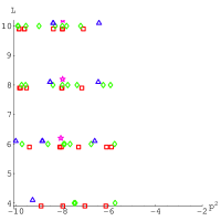
$\scriptstyle{\rm(a)}$  $\scriptstyle{\rm(b)}$

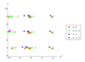
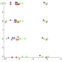
$\scriptstyle{\rm(c)}$  $\scriptstyle{\rm(d)}$

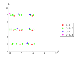
Figure 1: Zeros of scalar $\Delta^{\scriptscriptstyle(n)}_{+}(p^{2})$ (a), scalar $\Delta^{\scriptscriptstyle(n)}_{-}(p^{2})$ (b), vector $\Delta^{\scriptscriptstyle(n)}_{+}(p^{2})$ (c),vector $\Delta^{\scriptscriptstyle(n)}_{-}(p^{2})$ (d) at levels $L=4,\ldots,9$ up to $p^{2}=-10$.

We found that the determinants have zeros only on the negative $p^{2}$ axis, corresponding to physical (positive) values of $m^{2}=-p^{2}$. The first zeros (on the negative $p^{2}$ axis, closest to the origin) of the scalar even determinants are located around $p^{2}=-6$ (Graph (a) of Figure 1). However up to level 10 they are not stable yet. Their number keeps jumping as one increases the level: no multiple structure is detectable up to this level. We cannot therefore draw any conclusions about the fate of the Sen’s conjecture in the even scalar sector.

For scalars in the odd sector and vectors in both odd and even sectors there exists a first group of zeros on the negative $p^{2}$ axis which are closest to $p^{2}=0$ and well separated from other zeros located at more negatives values of $p^{2}$ (Graphs (b),(c),(d) of Figure 1). These groups of “almost degenerate” zeros become stable starting with level $L=4$ or $L=5$. As the level increases these zeros move on the $p^{2}$ axis but their number does not jump. The almost degenerate zeros of the scalar odd determinant are located around $p^{2}=-2$; those of the vector even determinant around $p^{2}=-4$; and those of vector odd determinant around $p^{2}=-6$. In all these three cases, the almost degenerate zeros form a reducible representation of the $SU(1,1)$ which is the sum of a scalar with $J=0$ , two doublets with $J=1/2$ and a vector with $J=1$. The associated Fadeev-Popov index vanishes

$$\sum_{J=0,1/2,1}(-1)^{2\,J}(2\,J+1)\,d_{J}=0$$ (4.16)

The observation which is important for our analysis is the following: the two zeros with $J=1/2$ do correspond to a single eigenvalues of the kinetic operator with a zero of order two. This seems to be unequivocal looking at the graphs of the vanishing eigenvalue that is reported, for level 10 or 9 in Figure 2. The conclusion is that the two doublets with $J=1/2$ should correspond in the exact theory to a single zero with $d_{J}=2$.

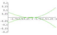
$\scriptstyle{\rm(a)}$  $\scriptstyle{\rm(b)}$

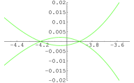
$\scriptstyle{\rm(c)}$

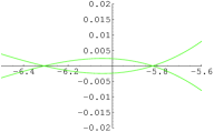
Figure 2: The vanishing eigenvalue of the kinetic operator for ghost number 1, at level 10 (or 9) in the scalar odd sector (a), vector even (b) and vector odd (c)

The almost degenerate zeros of the determinants for the scalar odd, vector even and vector odd sectors, are plotted, with the corresponding levels, in Figures 5,5,5. In the same plots we also show the linear fits of the zeros locations as function of the inverse of the level, $1/L$, for the different $SU(1,1)$ spins $J$.

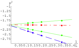
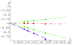
Figure 3: The first group of zeros of $\Delta^{\scriptscriptstyle(n)}_{-}(p^{2})$ in the scalar odd sector at $p^{2}\approx-2.0$ for levels $L=3,5,7,9$. $J=0$ dot-dashed-red, $J=1/2$ solid-green, $J=1$ dashed-blue.

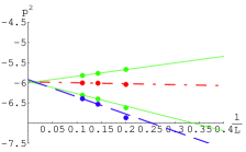
Figure 4: The first group of zeros of $\Delta^{\scriptscriptstyle(n)}_{+}(p^{2})$ in the vector even sector at $p^{2}\approx-4.0$ for levels $L=4,6,8,10$. $J=0$ dot-dashed-red, $J=1/2$ solid-green, $J=1$ dashed-blue.

Figure 5: The first group of zeros of $\Delta^{\scriptscriptstyle(n)}_{-}(p^{2})$ in the vector odd sector at $p^{2}\approx-6.0$ for levels $L=5,7,9$. $J=0$ dot-dashed-red, $J=1/2$ solid-green, $J=1$ dashed-blue.

The linearly extrapolated values of the zeros of the determinants for spins $J=0,1/2,1$ in the various Lorentz/twist-parity sectors are listed in Table 3.

Table 3: Determinant zeros extrapolated at $L=\infty$

Sector	J=0	J=1/2	J=1
scalar odd	-1.99172	-2.03279;  -1.97541	-2.04905
vector even	-3.98938	-3.99494;  -3.99087	-3.98803
vector odd	-5.97751	-5.96576;  -6.00275	-5.78701

Extrapolated zeros with different $J$ agree with remarkable accuracy. It is very tempting to conjecture from these data that the exact values for the degenerate zeros in the corresponding sectors are

$${m^{2}}_{\scriptscriptstyle scalar,-}=2.0$$

$${m^{2}}_{\scriptscriptstyle vector,+}=4.0$$

$${m^{2}}_{\scriptscriptstyle vector,-}=6.0$$

5 The action of ${\widetilde{Q}}$ on the zeros of ${\widetilde{L}}_{0}$

We found, numerically, that the kernels ${\widetilde{W}}_{\scriptscriptstyle n}$ of ${\widehat{L}}_{0}^{(n)}$ corresponding to multiplets of approximately degenerate propagators poles, form a singlet, a doublet and a triplet of the $SU(1,1)$ symmetry, in all sectors listed in Table 3. Let us denote by $v_{\pm 2}$ and $v_{\pm 1}$ the vectors that generate, respectively, the kernels ${\widetilde{W}}_{\scriptscriptstyle\pm 2}$ and ${\widetilde{W}}_{\scriptscriptstyle\pm 1}$. Let $v_{0}^{s}$ and $v_{0}^{t}$ be the vectors in ${\widetilde{W}}_{\scriptscriptstyle 0}$ that belong to, respectively, the singlet and the triplet of $SU(1,1)$. One has

$$J_{+}\,v_{0}^{s}=0\quad v_{0}^{t}=J_{+}\,v_{-2}\quad v_{2}=J_{+}\,v_{0}^{t}\quad J_{+}\,v_{2}=0$$

$$v_{1}=J_{+}\,v_{-1}\qquad J_{+}\,v_{1}=0$$ (5.1)

$J_{+}$ commutes both with ${\widetilde{L}}_{0}$ and with ${\widetilde{Q}}$. It follows that it commutes with ${\widehat{M}}$, ${\widehat{L}}_{0}$, ${\widehat{D}}$, ${\widehat{Z}}$ and $\check{Z}$. Therefore $J_{+}$ maps not only ${\widetilde{W}}_{\scriptscriptstyle n}$ into ${\widetilde{W}}_{\scriptscriptstyle n+2}$ but also $\check{W}_{\scriptscriptstyle n}$ into $\check{W}_{\scriptscriptstyle n+2}$.

The goal of this Section is to evaluate the dimensions of the tilde and check relative cohomologies

$${\tilde{\mathrm{n}}}^{\scriptscriptstyle(n)}\equiv\dim{\tilde{\mathrm{h}}}^{\scriptscriptstyle(n)}\qquad{\check{\mathrm{n}}}^{\scriptscriptstyle(n)}\equiv\dim{\check{\mathrm{h}}}^{\scriptscriptstyle(n)}$$ (5.2)

As explained above, our numerical computations indicate that the dimensions of the kernels ${\widetilde{W}}_{\scriptscriptstyle n}$ of ${\widehat{L}}_{0}^{(n)}$ in the exact theory are

$$\dim{\widetilde{W}}_{\scriptscriptstyle 0}=2\quad\dim{\widetilde{W}}_{\scriptscriptstyle\pm 1}=1\quad\dim{\widetilde{W}}_{\scriptscriptstyle\pm 2}=1\quad\dim{\widetilde{W}}_{\scriptscriptstyle\pm n}=0\quad{\rm for}\;n\geq 3$$ (5.3)

Therefore, for the same values of $p^{2}$, the relative indices are

$$\mathrm{index}\,\tilde{\mathrm{h}}=\mathrm{index}\,\check{\mathrm{h}}=\sum_{n}(-1)^{n}\dim{\widetilde{W}}_{\scriptscriptstyle n}=2$$ (5.4)

while the Fadeev-Popov index vanishes and

$${\cal H}^{\scriptscriptstyle(0)}({\widetilde{Q}})={\cal H}^{\scriptscriptstyle(1)}({\widetilde{Q}})=0$$ (5.5)

in agreement with Sen’s conjecture. When ${\cal H}^{\scriptscriptstyle(0)}({\widetilde{Q}})={\cal H}^{\scriptscriptstyle(1)}({\widetilde{Q}})=0$ the long sequence (3.17) breaks into the short exact sequence

$$0\;{\mathop{\longrightarrow}^{\pi}}\;{\check{\mathrm{h}}}^{\scriptscriptstyle(-1)}\;{\mathop{\longrightarrow}^{\widetilde{\cal D}}}\;{\tilde{\mathrm{h}}}^{\scriptscriptstyle(1)}\;{\mathop{\longrightarrow}^{\imath}}\;0$$ (5.6)

and into the two semi-infinite exact sequences

$$\!\!\!\!\!\!\!\!\cdots\;{\mathop{\longrightarrow}^{\pi}}\;{\check{\mathrm{h}}}^{\scriptscriptstyle(-3)}\;{\mathop{\longrightarrow}^{\widetilde{\cal D}}}\;{\tilde{\mathrm{h}}}^{\scriptscriptstyle(-1)}\;{\mathop{\longrightarrow}^{\imath}}\;{\cal H}^{\scriptscriptstyle(-1)}({\widetilde{Q}})\;{\mathop{\longrightarrow}^{\pi}}\;{\check{\mathrm{h}}}^{\scriptscriptstyle(-2)}\;{\mathop{\longrightarrow}^{\widetilde{\cal D}}}\;{\tilde{\mathrm{h}}}^{\scriptscriptstyle(0)}\;{\mathop{\longrightarrow}^{\imath}}\;0$$

$$\!\!\!0\;{\mathop{\longrightarrow}^{\pi}}\;{\check{\mathrm{h}}}^{\scriptscriptstyle(0)}\;{\mathop{\longrightarrow}^{\widetilde{\cal D}}}\;{\tilde{\mathrm{h}}}^{\scriptscriptstyle(2)}\;{\mathop{\longrightarrow}^{\imath}}\;{\cal H}^{\scriptscriptstyle(-1)}({\widetilde{Q}})\;{\mathop{\longrightarrow}^{\pi}}\;{\check{\mathrm{h}}}^{\scriptscriptstyle(1)}\;{\mathop{\longrightarrow}^{\widetilde{\cal D}}}\;{\tilde{\mathrm{h}}}^{\scriptscriptstyle(3)}\;{\mathop{\longrightarrow}^{\imath}}\;\cdots$$

(5.7)

From (5.6) one obtains

$${\tilde{\mathrm{h}}}^{\scriptscriptstyle(1)}={\check{\mathrm{h}}}^{\scriptscriptstyle(-1)}$$ (5.8)

and this should hold for any $p^{2}$ — if Sen’s conjecture is true.

Eq. (5.3) implies that the semi-infinite exact sequences (5.7) break up into finite sequences

$$0\;{\mathop{\longrightarrow}^{\widetilde{\cal D}}}\;{\tilde{\mathrm{h}}}^{\scriptscriptstyle(-1)}\;{\mathop{\longrightarrow}^{\imath}}\;{\cal H}^{\scriptscriptstyle(-1)}({\widetilde{Q}})\;{\mathop{\longrightarrow}^{\pi}}\;{\check{\mathrm{h}}}^{\scriptscriptstyle(-2)}\;{\mathop{\longrightarrow}^{\widetilde{\cal D}}}\;{\tilde{\mathrm{h}}}^{\scriptscriptstyle(0)}\;{\mathop{\longrightarrow}^{\imath}}\;0$$

$$0\;{\mathop{\longrightarrow}^{\pi}}\;{\check{\mathrm{h}}}^{\scriptscriptstyle(0)}\;{\mathop{\longrightarrow}^{\widetilde{\cal D}}}\;{\tilde{\mathrm{h}}}^{\scriptscriptstyle(2)}\;{\mathop{\longrightarrow}^{\imath}}\;{\cal H}^{\scriptscriptstyle(2)}({\widetilde{Q}})\;{\mathop{\longrightarrow}^{\pi}}\;{\check{\mathrm{h}}}^{\scriptscriptstyle(1)}\;{\mathop{\longrightarrow}^{\widetilde{\cal D}}}\;0$$

$$0\;{\mathop{\longrightarrow}^{\widetilde{\cal D}}}\;{\tilde{\mathrm{h}}}^{\scriptscriptstyle(-2)}\;{\mathop{\longrightarrow}^{\imath}}\;{\cal H}^{\scriptscriptstyle(-2)}({\widetilde{Q}})\;{\mathop{\longrightarrow}^{\pi}}\;0$$

$$0\;{\mathop{\longrightarrow}^{\imath}}\;{\cal H}^{\scriptscriptstyle(3)}({\widetilde{Q}})\;{\mathop{\longrightarrow}^{\pi}}\;{\check{\mathrm{h}}}^{\scriptscriptstyle(2)}\;{\mathop{\longrightarrow}^{\widetilde{\cal D}}}\;0$$ (5.9)

Hence, we obtain

$${\cal H}^{\scriptscriptstyle(-2)}({\widetilde{Q}})={\cal H}^{\scriptscriptstyle(3)}({\widetilde{Q}})={\tilde{\mathrm{h}}}^{\scriptscriptstyle(-2)}={\check{\mathrm{h}}}^{\scriptscriptstyle(2)}$$ (5.10)

from the last two sequences above, while the first two give

$$\dim{\cal H}^{\scriptscriptstyle(-1)}({\widetilde{Q}})={\tilde{\mathrm{n}}}^{\scriptscriptstyle(-1)}+{\check{\mathrm{n}}}^{\scriptscriptstyle(-2)}-{\tilde{\mathrm{n}}}^{\scriptscriptstyle(0)}=\dim{\cal H}^{\scriptscriptstyle(2)}({\widetilde{Q}})=-{\check{\mathrm{n}}}^{\scriptscriptstyle(0)}+{\tilde{\mathrm{n}}}^{\scriptscriptstyle(2)}+{\check{\mathrm{n}}}^{\scriptscriptstyle(1)}$$ (5.11)

Eqs. (5.8), (5.10), and (5.11) establish the following relations between the dimensions of the relative tilde and check cohomologies:

$${\check{\mathrm{n}}}^{\scriptscriptstyle(-1)}={\tilde{\mathrm{n}}}^{\scriptscriptstyle(1)}\qquad{\check{\mathrm{n}}}^{\scriptscriptstyle(0)}=2+{\tilde{\mathrm{n}}}^{\scriptscriptstyle(1)}-{\tilde{\mathrm{n}}}^{\scriptscriptstyle(-2)}+{\check{\mathrm{n}}}^{\scriptscriptstyle(1)}-{\check{\mathrm{n}}}^{\scriptscriptstyle(-2)}\qquad{\check{\mathrm{n}}}^{\scriptscriptstyle(2)}={\tilde{\mathrm{n}}}^{\scriptscriptstyle(-2)}$$ (5.12)

We now want to look for solutions of the equations (5.4-5.11) with

$${\tilde{\mathrm{n}}}^{\scriptscriptstyle(0)},{\check{\mathrm{n}}}^{\scriptscriptstyle(0)}=0,1,2,\qquad{\tilde{\mathrm{n}}}^{\scriptscriptstyle(1)},{\check{\mathrm{n}}}^{\scriptscriptstyle(1)},{\tilde{\mathrm{n}}}^{\scriptscriptstyle(2)},{\check{\mathrm{n}}}^{\scriptscriptstyle(2)}=0,1$$ (5.13)

Moreover, relations (3.26) and (3.31) require that

$${\check{\mathrm{n}}}^{\scriptscriptstyle(-2)}\leq{\tilde{\mathrm{n}}}^{\scriptscriptstyle(-2)}\quad{\rm and}\quad{\check{\mathrm{n}}}^{\scriptscriptstyle(2)}\geq{\tilde{\mathrm{n}}}^{\scriptscriptstyle(2)}$$ (5.14)

The most general action of ${\widehat{M}}$ on the kernel of ${\widehat{L}}_{0}$ takes the form

$${\widehat{M}}\,v_{-2}=\mu\,v_{-1}\qquad\qquad{\widehat{M}}\,v_{2}=0$$

$${\widehat{M}}\,v_{-1}=\alpha\,v_{0}^{s}+\beta\,v_{0}^{t}\qquad{\widehat{M}}\,v_{1}=\beta\,v_{2}$$

$${\widehat{M}}\,v_{0}^{s}=\gamma\,v_{1}\qquad{\widehat{M}}\,v_{0}^{t}={\widehat{M}}\,J_{+}v_{-2}=\mu\,v_{1}$$ (5.15)

where $\mu$, $\alpha$, $\beta$ and $\gamma$ are numbers. (Without loss of generality we can assume these numbers to be real, since their phases can be reabsorbed into the normalizations of the vectors $v_{-n}$). ${\widehat{M}}^{2}=0$ is equivalent to the relations

$$\mu\,\alpha=\mu\,\beta=0$$

$$\alpha\,\gamma=\beta\,\gamma=0$$ (5.16)

The possible solutions of (5.16) are

a) $\alpha=\beta=\gamma=\mu=0$

b) $\mu\not=0$, $\alpha=\beta=0$

c) $\mu=0$, $\gamma=0$, $(\alpha,\beta)\not=(0,0)$

d) $\mu=\alpha=\beta=0$, $\gamma\not=0$

Only d), however, is compatible with the constraints that come from the sequence (5.9) and the fact that $J_{+}$ commutes with ${\widetilde{Q}}$. Let us show why.

Solution a) leads to

$${\tilde{\mathrm{n}}}^{\scriptscriptstyle(-2)}=1\quad{\tilde{\mathrm{n}}}^{\scriptscriptstyle(-1)}=1\quad{\tilde{\mathrm{n}}}^{\scriptscriptstyle(0)}=2\quad{\tilde{\mathrm{n}}}^{\scriptscriptstyle(1)}=1\quad{\tilde{\mathrm{n}}}^{\scriptscriptstyle(2)}=1$$ (5.17)

Since ${\tilde{\mathrm{n}}}^{\scriptscriptstyle(0)}-{\tilde{\mathrm{n}}}^{\scriptscriptstyle(-1)}=1$ it follows from (5.11) that

$${\check{\mathrm{n}}}^{\scriptscriptstyle(-2)}=1\qquad\dim{\cal H}^{\scriptscriptstyle(-1)}({\widetilde{Q}})=0$$ (5.18)

If ${\cal H}^{\scriptscriptstyle(-1)}({\widetilde{Q}})=0$ the first two sequences in (5.9) split farther and give

$${\check{\mathrm{n}}}^{\scriptscriptstyle(1)}={\tilde{\mathrm{n}}}^{\scriptscriptstyle(-1)}=0$$ (5.19)

in conflict with Eq. (5.17) above.

Solution b) leads to the following values for the tilde cohomologies

$${\tilde{\mathrm{n}}}^{\scriptscriptstyle(-2)}=0\quad{\tilde{\mathrm{n}}}^{\scriptscriptstyle(-1)}=0\quad{\tilde{\mathrm{n}}}^{\scriptscriptstyle(0)}=1\quad{\tilde{\mathrm{n}}}^{\scriptscriptstyle(1)}=0\quad{\tilde{\mathrm{n}}}^{\scriptscriptstyle(2)}=1$$ (5.20)

Again, ${\tilde{\mathrm{n}}}^{\scriptscriptstyle(0)}-{\tilde{\mathrm{n}}}^{\scriptscriptstyle(-1)}=1$ and therefore, as in (5.18) ${\check{\mathrm{n}}}^{\scriptscriptstyle(-2)}=1$. But this is inconsistent with the inequalities (5.14) which require ${\check{\mathrm{n}}}^{\scriptscriptstyle(-2)}\leq{\tilde{\mathrm{n}}}^{\scriptscriptstyle(-2)}=0$.

Two different sets of values for tilde cohomologies are a priori possible in case of solution c):

$${\tilde{\mathrm{n}}}^{\scriptscriptstyle(-2)}=1\quad{\tilde{\mathrm{n}}}^{\scriptscriptstyle(-1)}=0\quad{\tilde{\mathrm{n}}}^{\scriptscriptstyle(0)}=1\quad{\tilde{\mathrm{n}}}^{\scriptscriptstyle(1)}=n\quad{\tilde{\mathrm{n}}}^{\scriptscriptstyle(2)}=n$$ (5.21)

with $n=1$ if $\beta=0$ and $n=0$ if $\beta\not=0$. In both cases, ${\tilde{\mathrm{n}}}^{\scriptscriptstyle(0)}-{\tilde{\mathrm{n}}}^{\scriptscriptstyle(-1)}=1$, and therefore Eqs. (5.18) and (5.19) hold as well. Therefore the values of the check cohomologies are

$${\check{\mathrm{n}}}^{\scriptscriptstyle(-2)}=1\quad{\check{\mathrm{n}}}^{\scriptscriptstyle(-1)}=n\quad{\check{\mathrm{n}}}^{\scriptscriptstyle(0)}=n\quad{\check{\mathrm{n}}}^{\scriptscriptstyle(1)}=0\quad{\check{\mathrm{n}}}^{\scriptscriptstyle(2)}=1$$ (5.22)

However, $n=1={\check{\mathrm{n}}}^{\scriptscriptstyle(-1)}$ requires $\alpha=\beta=0$, otherwise ${\widehat{M}}$ would have no kernel on $\check{W}_{\scriptscriptstyle-1}\subset{\widetilde{W}}_{\scriptscriptstyle-1}$. This reduces again to solution a), which we have already ruled out. Therefore $n=0$. Since ${\check{\mathrm{n}}}^{\scriptscriptstyle(-2)}=1$, $v_{-2}\in\check{W}_{\scriptscriptstyle-2}$. Thus $v_{0}^{t}\in\check{W}_{\scriptscriptstyle 0}$ and $v_{2}\in\check{W}_{\scriptscriptstyle 2}$. ${\check{\mathrm{n}}}^{\scriptscriptstyle(0)}=0$ dictates that $v_{0}^{t}$ be trivial in check cohomology. Therefore, $\alpha=0$ and

$${\widehat{M}}\,v_{-1}=\beta\,v_{0}^{t}$$ (5.23)

where $\beta\not=0$ and $v_{-1}\in\check{W}_{\scriptscriptstyle-1}$. As $J_{+}$ sends $\check{W}_{\scriptscriptstyle-1}$ to $\check{W}_{\scriptscriptstyle 1}$ we conclude that

$$v_{1}=J_{+}\,v_{-1}\in\check{W}_{\scriptscriptstyle 1}$$ (5.24)

We reached a contradiction: $v_{2}\in\check{W}_{\scriptscriptstyle 2}$, $v_{1}\in\check{W}_{\scriptscriptstyle 1}$ and $\beta\,v_{2}={\widehat{M}}\,v_{1}$ means that ${\check{\mathrm{n}}}^{\scriptscriptstyle(2)}=0$, in conflict with (5.22).

We are left therefore with solution d), for which

$${\tilde{\mathrm{n}}}^{\scriptscriptstyle(-2)}=1\quad{\tilde{\mathrm{n}}}^{\scriptscriptstyle(-1)}=1\quad{\tilde{\mathrm{n}}}^{\scriptscriptstyle(0)}=1\quad{\tilde{\mathrm{n}}}^{\scriptscriptstyle(1)}=0\quad{\tilde{\mathrm{n}}}^{\scriptscriptstyle(2)}=1$$ (5.25)

The first sequence in (5.9) implies that ${\check{\mathrm{n}}}^{\scriptscriptstyle(-2)}$ does not vanish — since ${\tilde{\mathrm{n}}}^{\scriptscriptstyle(0)}=1$. Thus ${\check{\mathrm{n}}}^{\scriptscriptstyle(-2)}=1$. Therefore $v_{-2}\in\check{W}_{\scriptscriptstyle-2}$ and $v_{0}^{t}=J_{+}\,v_{-2}\in\check{W}_{\scriptscriptstyle 0}$. Since ${\widehat{M}}\,v_{0}^{t}=0$ and ${\widehat{M}}\,v_{-1}=$, we conclude that ${\check{\mathrm{n}}}^{\scriptscriptstyle(0)}=1$. This, together with the general relations (5.12), determines all of the check cohomologies:

$${\check{\mathrm{n}}}^{\scriptscriptstyle(-2)}=1\quad{\check{\mathrm{n}}}^{\scriptscriptstyle(-1)}=0\quad{\check{\mathrm{n}}}^{\scriptscriptstyle(0)}=1\quad{\check{\mathrm{n}}}^{\scriptscriptstyle(1)}=1\quad{\check{\mathrm{n}}}^{\scriptscriptstyle(2)}=1$$ (5.26)

To sum up, the action of the operators ${\widehat{M}}$ on the kernel ${\widetilde{W}}_{\scriptscriptstyle n}$ and the subspaces $\check{W}_{\scriptscriptstyle n}$ which are compatible with our sequence are

$${\widehat{M}}\,v_{\pm 2}=0\qquad{\widehat{M}}\,v_{\pm 1}=0\qquad{\widehat{M}}\,v_{0}^{t}=0\qquad{\widehat{M}}\,v_{0}^{s}=v_{1}$$

$$\check{W}_{\scriptscriptstyle\pm 2}=\{v_{\pm 2}\}\quad\check{W}_{\scriptscriptstyle-1}=0\quad\check{W}_{\scriptscriptstyle 1}=\{v_{1}\}\quad\check{W}_{\scriptscriptstyle 0}=\{v_{0}^{t}\}$$ (5.27)

Non-trivial representatives of ${\cal H}^{\scriptscriptstyle(-1)}({\widetilde{Q}})$ and ${\cal H}^{\scriptscriptstyle(-2)}({\widetilde{Q}})$ are $v_{-1}$ and $v_{-2}$, respectively. The dual non-empty cohomologies ${\cal H}^{\scriptscriptstyle(2)}({\widetilde{Q}})$ and ${\cal H}^{\scriptscriptstyle(3)}({\widetilde{Q}})$ have representatives

$$\phi_{2}=c_{0}\,v_{1}+\phi_{2}^{\prime}$$ (5.28)

and

$$\phi_{3}=c_{0}\,v_{2}+\phi_{3}^{\prime}$$ (5.29)

respectively, where $\phi_{2}^{\prime}$ and $\phi_{3}^{\prime}$ are given by

$$\quad{\widehat{Z}}\,v_{1}={\widehat{L}}_{0}\,\phi^{\prime}_{2}\qquad\quad{\widehat{Z}}\,v_{2}={\widehat{L}}_{0}\,\phi^{\prime}_{3}$$ (5.30)

Note that $\phi^{\prime}_{2}$ and $\phi^{\prime}_{3}$ are defined by these equations up to elements in the kernels of ${\widehat{L}}_{0}$ on ${\widetilde{W}}_{\scriptscriptstyle 2}$ and ${\widetilde{W}}_{\scriptscriptstyle 3}$. The latter is empty and the former is spanned by $v_{2}$: the exactness of the sequence (5.9) ensures that $v_{2}$ is trivial in the ${\widetilde{Q}}$ cohomology.

References

[1]
S. Giusto and C. Imbimbo, “Physical states at the tachyonic vacuum of
open string field theory,” Nucl. Phys. B 677, 52 (2004)
[arXiv:hep-th/0309164].
[2]
A. Sen, “Descent relations among bosonic D-branes,” Int. J. Mod. Phys. A 14, 4061 (1999) [arXiv:hep-th/9902105].
[3]
A. Sen,
“Universality of the tachyon potential,”
JHEP 9912, 027 (1999) [arXiv:hep-th/9911116].
[4]
E. Witten,
“Noncommutative Geometry And String Field Theory,”
Nucl. Phys. B 268, 253 (1986).
[5]
V. A. Kostelecky and S. Samuel,
“On A Nonperturbative Vacuum For The Open Bosonic String,”
Nucl. Phys. B 336, 263 (1990).
[6]
A. Sen and B. Zwiebach, “Tachyon condensation in string field theory,”
JHEP 0003, 002 (2000) [arXiv:hep-th/9912249].
[7]
N. Moeller and W. Taylor,
“Level truncation and the tachyon in open bosonic string field theory,”
Nucl. Phys. B 583, 105 (2000) [arXiv:hep-th/0002237].
[8]
D. Gaiotto and L. Rastelli,
“Experimental string field theory,”
arXiv:hep-th/0211012.
[9]
M. Schnabl,
“Analytic solution for tachyon condensation in open string field
theory,” arXiv:hep-th/0511286.
[10]
I. Ellwood and W. Taylor,
“Open string field theory without open strings,”
Phys. Lett. B 512, 181 (2001)
[arXiv:hep-th/0103085].
[11]
L. Rastelli, A. Sen and B. Zwiebach,
“String field theory around the tachyon vacuum,”
Adv. Theor. Math. Phys. 5, 353 (2002)
[arXiv:hep-th/0012251].
[12]
I. Ellwood, B. Feng, Y. H. He and N. Moeller,
“The identity string field and the tachyon vacuum,”
JHEP 0107, 016 (2001)
[arXiv:hep-th/0105024].
[13]
M. Bochicchio,
“Gauge Fixing For The Field Theory Of The Bosonic String,”
Phys. Lett. B 193, 31 (1987).
C. B. Thorn,
“Perturbation Theory For Quantized String Fields,
Nucl. Phys. B 287, 61 (1987).
[14]
R. Bott and L. W. Tu, “Differential Forms in Algebraic Topology,”
Springer-Verlag, New York, 1997.
[15]
M. Beccaria and C. Rampino,
“Level truncation and the quartic tachyon coupling,”
[arXiv:hep-th/0308059].
[16]
I. Ellwood and M. Schnabl,
“Proof of vanishing cohomology at the tachyon vacuum,”
arXiv:hep-th/0606142.
[17]
M. Schnabl,
“Wedge states in string field theory,”
JHEP 0301, 004 (2003).
[18]
L. Rastelli and B. Zwiebach,
“Tachyon potentials, star products and universality,”
JHEP 0109, 038 (2001).
[19]
I. Kishimoto and K. Ohmori,
“CFT description of identity string field: Toward derivation of the VSFT
action,”
JHEP 0205, 036 (2002).
[20]
B. Zwiebach, “Trimming the tachyon string field with SU(1,1),”
arXiv:hep-th/0010190.
[21]
I. Kishimoto and T. Takahashi,
“Open string field theory around universal solutions,”
Prog. Theor. Phys. 108, 591 (2002)
[arXiv:hep-th/0205275].