Effective potential at finite temperature in a constant hypermagnetic field: Ring diagrams in the Standard Model

Abstract

We study the symmetry breaking phenomenon in the standard model during the electroweak phase transition in the presence of a constant hypermagnetic field. We compute the finite temperature effective potential up to the contribution of ring diagrams in the weak field, high temperature limit and show that under these conditions, the phase transition becomes stronger first order.

I Introduction

The problem of baryogenesis is still one of the outstanding open questions in cosmology, despite the large amount of work devoted to find a viable explanation. The conditions for developing a baryon asymmetry in an initially symmetric universe were established by Sakharov in 1967 Sakharov and the search for a scenario to encompass them continues. These three well-known conditions are: (1) existence of interactions that violate baryon number; (2) C and CP violation and (3) departure from thermal equilibrium.

The Standard Model (SM) of electroweak interactions meets all these requirements, provided the electroweak phase transition (EWPT) be first order, since, at that stage of the universe evolution, this is the only possible source of departure from thermal equilibrium. Nonetheless, it is well known that neither the amount of CP violation within the minimal SM Gavela , nor the strength of the EWPT are enough to generate a sizable baryon number Kajantie1 .

During the EWPT, the Higgs field vacuum expectation value changes from zero (false vacuum) in the symmetric phase, to a finite value $\langle v\rangle$ (true vacuum) in the broken phase. This evolution is determined by the finite temperature effective potential of the theory, that develops a barrier between the two minima if the phase transition is first order. The temperature at which the two minima are degenerate is called the critical temperature $T_{c}$ and this instant is considered the beginning of the phase transition. From there on, the transition is accomplished through the nucleation, expansion and percolation of true vacuum bubbles in the background of false vacuum, leading to a departure from equilibrium conditions.

The existence of baryon number violation is realized in the SM by means of its vacuum structure through sphaleron mediated processes. The sphaleron Klinkhamer is a static and unstable solution of the field equations of non-Abelian gauge theories, corresponding to the top of the energy barrier between topologically distinct vacua, where the minima correspond to configurations with zero gauge field energy but different baryon number. Transitions are associated to baryon number $n_{B}-n_{\bar{B}}$ violation and can either induce or wash out a baryon asymmetry.

The above property of sphalerons makes the preservation of a given baryon asymmetry one of the most difficult conditions to meet during the baryogenesis process in the majority of the proposed scenarios. This requires that the baryon violating transition between different topological vacua is suppressed in the broken phase, when the universe returns to thermal equilibrium. In other words, the sphaleron transitions must be slow compared to the expansion rate of the universe and this in turn translates into the condition $\langle v\rangle/T_{c}\geq 1.0-1.5$ Kajantie1 . Although the above is an estimate emerging from approximate calculations, it is nowadays widely accepted and has proven to be a rather difficult condition to meet.

Although there have been several attempts to link the baryogenesis process to the EWPT reviewsEWPT ; Petropoulos in general these all share the characteristic that the Sakharov conditions are only partially met. Here we want to further explore the possibility to embed the baryogenesis process in the EWPT scenario, including the effect of an extra ingredient: the possible presence of primordial magnetic fields. Before the EWPT, magnetic fields couple to matter through the particle’s hypercharge and thus properly receive the name of hypermagnetic fields.

Magnetic fields seem to pervade the entire universe and their generation may be either primordial or associated to the process of structure formation. They have been observed in galaxies, clusters, intracluster medium and high redshift objects 31 . In order to distinguish between primordial and protogalactic fields, it is useful to search for their imprint on the cosmic microwave background radiation (CMBR). A homogeneous magnetic field would give rise to a dipole anisotropy in the background radiation, on this basis, Cosmic Background Explorer (COBE) results give an upper bound on the present equivalent field strength of $B_{0}\lesssim 10^{-9}$ G Barrow . An upper limit to the field strength of $B_{0}\lesssim 4.7\times 10^{-9}$ G at the present scale of 1 Mpc is obtained by an analysis that includes small scale CMBR anisotropies from Wilkinson Microwave Anisotropy Probe (WMAP), Cosmic Background Imager (CBI) and Arc Minute Cosmology Bolometer Array Receiver (ACBAR) Yamazaki . On the other hand, tangled random fields on small scales could reach up to $\sim 10^{-6}$ G Barrow2 . Nucleosynthesis also imposes limits on primordial magnetic fields since they have an influence on both the universe expansion rate and the electron quantum statistics. The observed helium abundance implies $B\lesssim 10^{12}$ G at scales greater than 10 cm at the end of nucleosynthesis Grasso .

Although at present there is no conclusive evidence about the origin of magnetic fields, their existence prior to the EWPT cannot certainly be ruled out making it important to investigate their effect on the baryogenesis process elreview . In fact, it has been shown that these fields provide mechanisms to affect all the Sakharov conditions: In the presence of a magnetic field, the phase transition becomes stronger first order in analogy to the case of a type I superconductor, where the Meissner effect brings the phase transition from second to first order Giovannini ; Elmfors ; Kajantie ; it has also been shown that extra CP violation is obtained from the segregation of axial charge during the reflection and transmission of fermions through the vacuum bubbles due to the chiral nature of their coupling to the hypermagnetic field Pallares ; finally, regarding the sphaleron transitions the presence of a magnetic field works against the preservation of a baryon asymmetry due to the coupling between the sphaleron dipole moment and the magnetic field that lowers the energy barrier between topologically distinct minima Dario .

The effect of magnetic fields on the EWPT has been analytically studied both classically  Giovannini and to one-loop order Elmfors , as well as by means of lattice simulations Kajantie . These calculations all agree that the strength of the phase transition is enhanced by the presence of hypermagnetic fields, although the ratio $\langle v\rangle/T_{c}$ does not reach the desired value, for a large Higgs boson mass. On the other hand, other analytical approaches where the SM finite temperature effective potential is studied for the case of strong magnetic fields Skalozub1 ; Skalozub2 , reach the conclusion that these fields inhibit the first order phase transition and attribute the result to the contribution of light fermion masses which are generally neglected in other computations.

In this work we concentrate on studying the relation between the presence of a large scale magnetic field and the dynamics of the EWPT by computing the SM finite temperature effective potential in a constant hypermagnetic field up to the contribution of ring diagrams, that have been shown to be crucial for the description of the long wavelength properties of the theory Carrington . We carry out a systematic calculation of each SM sector showing that the major contribution producing an enhancement of the EWPT comes from the Higgs and gauge boson sectors and that fermions do not act against this behavior. Working in the limit where the magnetic field is weak, we find an enhanced value of the ratio $\langle v\rangle/T_{c}$.

The paper is organized as follows: In Sec. II we lay down the formalism to include weak magnetic fields in the computation of hypercharged particle propagators. In Sec. III we write down the SM using the degrees of freedom in the symmetric phase. In Sec. IV, we work with these degrees of freedom to compute particle self energies that are used in Sec. V to compute the SM effective potential up to the contributions of ring diagrams. In Sec. VI we study this effective potential as a function of the Higgs vacuum expectation value and show that the order of the EWPT becomes stronger first order in the presence of the hypermagnetic field. Finally, we conclude and discuss our results in Sec. VII and leave for the appendix the computation of some intermediate results of the analysis.

II Charged particle propagators in the presence of a Hypermagnetic Field

We work with the degrees of freedom of the SM in the symmetric phase, where the external (hyper)magnetic field belongs to the $U(1)_{Y}$ group. To include the effect of the external field, we use Schwinger’s proper time method Schwinger . In the symmetric phase, we have only two kinds of hypercharged particles that couple to the external field namely, scalars and fermions, whose propagators are

$$D_{H}(x,x^{\prime})=\phi(x,x^{\prime})\int\frac{d^{4}K}{(2\pi)^{4}}e^{-ik\cdot(x-x^{\prime})}D_{H}(k),$$ (1)

$$S_{H}(x,x^{\prime})=\phi(x,x^{\prime})\int\frac{d^{4}K}{(2\pi)^{4}}e^{-ik\cdot(x-x^{\prime})}S_{H}(k),$$ (2)

respectively. The phase factor $\phi(x,x^{\prime})$, that breaks translation invariance, is given by

$$\phi(x,x^{\prime}) \equiv e^{i{\mbox{{\bf\tiny{Y}}}}\int^{x}_{x^{\prime}}d\xi^{\mu}\left[B^{{\mbox{\tiny{ext}}}}_{\mu}+\frac{1}{2}F_{\mu\nu}(\xi-x^{\prime})^{\nu}\right]},$$ (3)

where the vector potential $B^{{\mbox{\tiny{ext}}}}_{\mu}=\frac{H}{2}(0,y,-x,0)$ gives rise to a constant hypermagnetic field of strength $H$ along the $\hat{z}$ axis and $F^{{\mbox{\tiny{ext}}}}_{\mu\nu}=\partial_{\mu}B^{{\mbox{\tiny{ext}}}}_{\nu}-\partial_{\nu}B^{{\mbox{\tiny{ext}}}}_{\mu}$ is the external field strength tensor.

The momentum dependent functions $D_{H}(k)$ and $S_{H}(k)$ are given by

$$iD_{H}(k) = \int_{0}^{\infty}\frac{ds}{\cos{{\mbox{{\bf\scriptsize{Y}}}}Hs}}$$ (4)

$$\times \exp\left\{is(k_{||}^{2}-k_{\bot}^{2}\frac{\tan{{\mbox{{\bf\scriptsize{Y}}}}H{s}}}{{\mbox{{\bf\scriptsize{Y}}}}Hs}-m^{2}+i\epsilon)\right\},$$

$$iS_{H}(k) = \int_{0}^{\infty}\frac{ds}{\cos{{\mbox{{\bf\scriptsize{Y}}}}Hs}}$$ (5)

$$\times \exp\left\{is(k_{||}^{2}-k_{\bot}^{2}\frac{\tan{{\mbox{{\bf\scriptsize{Y}}}}H{s}}}{{\mbox{{\bf\scriptsize{Y}}}}Hs}-m^{2}+i\epsilon)\right\}$$

$$\times \left[(m_{f}-{\not\!k}_{||})e^{i{\mbox{{\bf\tiny{Y}}}}Hs\sigma_{3}}-\frac{{\not\!k_{\bot}}}{\cos{{\mbox{{\bf\scriptsize{Y}}}}Hs}}\right],$$

where Y is the particle’s hypercharge and we use the notation $k_{||}^{2}=k_{0}^{2}-k_{3}^{2}$ and $k_{\perp}^{2}=k_{1}^{2}+k_{2}^{2}$.

Since the gauge bosons do not couple to the external field their propagator is given by

$$iD^{\mu\nu}_{ab}(k)=-i\left\{\frac{g^{\mu\nu}-(1-\xi)\frac{k^{\mu}k^{\nu}}{k^{2}-\xi m_{G}^{2}}}{k^{2}-m_{G}^{2}+i\epsilon}\right\}_{ab}$$ (6)

where $a,b=1,2,3,4$ and the first three values correspond to the $SU(2)_{L}$ fields and the fourth to the $U(1)_{Y}$ field. Notice that the matrix $m_{G}^{2}$ is not diagonal in the basis of the weak-interacting fields in the symmetric phase.

It has been show that, by deforming the contour of integration, Eqs. (4) and (5) can be written as nosotros ; Tzuu

$$iD_{H}(k)=2i\sum_{l=0}^{\infty}\frac{(-1)^{l}L_{l}(\frac{2k_{\perp}^{2}}{{\mbox{{\bf\tiny{Y}}}}H})\exp\left\{-\frac{k^{2}_{\perp}}{{\mbox{{\bf\tiny{Y}}}}H}\right\}}{k^{2}_{||}-(2l+1){\mbox{{\bf\scriptsize{Y}}}}H-m^{2}+i\epsilon},$$ (7)

$$iS_{H}(k)=i\sum^{\infty}_{l=0}\frac{d_{l}(\frac{k_{\perp}^{2}}{{\mbox{{\bf\tiny{Y}}}}H})D+d^{\prime}_{l}(\frac{k_{\perp}^{2}}{{\mbox{{\bf\tiny{Y}}}}H})\bar{D}}{k^{2}_{||}-2l{\mbox{{\bf\scriptsize{Y}}}}H-m_{f}^{2}+i\epsilon}+\frac{{\not\!k_{\bot}}}{k^{2}_{\perp}},$$ (8)

where $d_{l}(\alpha)\equiv(-1)^{n}e^{-\alpha}L^{-1}_{l}(2\alpha)$, $d^{\prime}_{n}=\partial d_{n}/\partial\alpha$,

$$D = (m_{f}+{\not\!k_{||}})+{\not\!k_{\perp}}\frac{m_{f}^{2}-k^{2}_{||}}{{k^{2}_{\perp}}},$$

$$\bar{D} = \gamma_{5}{\not\!u}{\not\!b}(m_{f}+{\not\!k_{||}}),$$ (9)

$L_{l}$, $L_{l}^{m}$ are Laguerre and Associated Laguerre polynomials, respectively, and $u^{\mu}$, $b^{\mu}$ are four-vectors describing the plasma rest frame and the direction of the hypermagnetic field, respectively.

In order to set the appropriate hierarchy of energy scales we resort to qualitative cosmological bounds on the possible strength of primordial magnetic fields during the EWPT. CMBR sets stringent bounds on large scale primordial fields but no so much stringent when the fields are tangled. This dependence on the scale makes it difficult to extrapolate these bounds down to the EWPT epoch. We use instead the requirement that the magnetic energy density $\rho_{mag}\sim B^{2}$ should be smaller than the overall radiation energy density $\rho_{rad}\sim T^{4}$ at nucleosynthesis, in order to preserve the estimated abundances of light elements. With this, one obtains the simple bound $B\lesssim T^{2}$ Maartens .

On the other hand stability conditions against the formation of $W$-condensate indicate Ambjorn that the field strength is also weak compared to the square of the $W$ mass, $m_{W}^{2}$. Notice however that when thermal corrections are taken into account, this bound could be avoided Skalozub1 ; Skalozub2 .

We work explicitly with the assumption that the hierarchy of scales

$${\mbox{{\bf\scriptsize{Y}}}}H\ll m^{2}\ll T^{2},$$ (10)

is obeyed, were we consider $m$ as a generic mass of the problem at the electroweak scale.

We can thus perform a weak field expansion in Eqs. (7) and (8) which allows to carry out the summation over Landau levels to write the scalar and fermion propagators as power series in ${\mbox{{\bf\scriptsize{Y}}}}H$, that up to order $({\mbox{{\bf\scriptsize{Y}}}}H)^{2}$ read as nosotros ; Tzuu

$$D(k)_{H}=\frac{1}{k^{2}-m^{2}}\left(1-\frac{({\mbox{{\bf\scriptsize{Y}}}}H)^{2}}{(k^{2}-m^{2})^{2}}-\frac{2({\mbox{{\bf\scriptsize{Y}}}}H)^{2}k_{\perp}^{2}}{(k^{2}-m^{2})^{3}}\right),$$

(11)

and

$${S(k)_{H}}=\frac{{\not\!k}+m_{f}}{{\not\!k}^{2}-m_{f}^{2}}+\frac{\gamma_{5}{\not\!u}{\not\!b}(k_{||}+m_{f})({\mbox{{\bf\scriptsize{Y}}}}H)}{(k^{2}-m_{f}^{2})^{3}}$$

$$-\frac{2({\mbox{{\bf\scriptsize{Y}}}}H)^{2}k_{\perp}^{2}}{(k^{2}-m_{f}^{2})^{4}}(m_{f}+{\not\!k_{||}}+{\not\!k_{\perp}}\frac{m_{f}^{2}-k_{||}^{2}}{k_{\perp}^{2}}),$$ (12)

respectively.

There is an analogous result for gauge bosons, but since in the symmetric phase these do not couple to the external hypermagnetic field, we do not need to account for them.

III Standard Model

In order to consider all the contributions to the SM effective potential, we write the Lagrangian for each sector.

The Lagrangian for the Higgs sector is

$$\mathcal{L}_{H}=(D_{\mu}\Phi)^{\dagger}(D^{\mu}\Phi)+c^{2}(\Phi^{\dagger}\Phi)-\lambda(\Phi^{\dagger}\Phi)^{2},$$ (13)

where $D_{\mu}=\partial_{\mu}+ig\frac{\tau^{a}}{2}{A^{a}_{\mu}}+i\frac{g^{\prime}{\mbox{{\bf\scriptsize{Y}}}}}{2}B^{\prime}_{\mu}$, $\tau^{a}$ are the Pauli matrices, $B^{\prime}_{\mu}=B_{\mu}+B^{\mbox{\tiny{ext}}}_{\mu}$ and $A^{a}_{\mu}$, $B_{\mu}$ are the $SU(2)_{L}$ and $U(1)_{Y}$ gauge bosons, respectively. To allow for spontaneous symmetry breaking the mass parameter $c$ must satisfy $c^{2}>0$.

The Higgs field is a complex doublet with $\mbox{\bf\scriptsize{Y}}=+1$

$$\Phi=\frac{1}{\sqrt{2}}\left(\begin{array}[]{cc}&\phi_{3}+i\phi_{4}\\ &\phi_{1}+i\phi_{2}\end{array}\right),$$ (16)

where $\phi_{i}$ are real scalar fields. We take $\phi_{1}$ as the physical Higgs field that develops a vacuum expectation value $v$. Extremizing the tree level potential, the parameter $c$ is related to the classical minimum $v_{class}$ by

$$c^{2}=\lambda v_{class}^{2}.$$ (17)

For the Higgs field hypercharge conjugate doublet we use ${\tilde{\Phi}}=i\sigma_{2}\Phi^{*}$.

The kinetic energy from the $SU(2)_{L}$ and $U(1)_{Y}$ gauge bosons is

$$\mathcal{L}_{gb}= -\frac{1}{4}{\bf F}^{\mu\nu}\cdot{\bf F}_{\mu\nu}-\frac{1}{4}F^{\prime\mu\nu}F^{\prime}_{\mu\nu},$$ (18)

where

$${\bf F}_{\mu\nu} = \partial_{\mu}{\bf A_{\nu}}-\partial_{\nu}{\bf A}_{\mu}-g{\bf A}_{\mu}\times{\bf A}_{\nu}$$

$$F^{\prime}_{\mu\nu} = \partial_{\mu}B^{\prime}_{\nu}-\partial_{\nu}B^{\prime}_{\mu}.$$ (19)

The Lagrangian for the fermion sector is

$$\mathcal{L}_{f}= \overline{\Psi}_{R}\left(i{\not\!\partial}-\frac{g^{\prime}}{2}{\mbox{{\bf\scriptsize{Y}}}}{\not\!\!B^{\prime}}\right)\Psi_{R}+$$ (20)

$$\overline{\Psi}_{L}\left(i{\not\!\partial}-\frac{g^{\prime}}{2}{\mbox{{\bf\scriptsize{Y}}}}{\not\!\!B^{\prime}}-\frac{g}{2}{\bf\tau}\cdot\bf{{\not\!\!A}}\right)\Psi_{L},$$

where $\Psi_{L}=\frac{1}{2}(1-\gamma_{5})\Psi$ is an $SU(2)$ doublet of left-handed fermions and $\Psi_{R}=\frac{1}{2}(1+\gamma_{5})\Psi$ is an $SU(2)$ singlet of right-handed fermions.

We work in the limit that all fermion masses except the top quark mass are negligible, so that the main contribution to the Yukawa sector is

$$\mathcal{L}_{Yukawa}=f\overline{q_{L}}{\tilde{\Phi}}{t}_{R}+h.c.$$ (21)

Finally, in the $R_{\xi}$ gauge, the gauge fixing Lagrangian is

$$\mathcal{L}_{gf}= - \frac{1}{2\xi}(\partial^{\mu}A_{\mu}^{i}-\frac{1}{2}\xi gv\phi^{i})^{2}-$$ (22)

$$\frac{1}{2\xi}(\partial^{\mu}B_{\mu}-\frac{1}{2}\xi g^{\prime}v\phi_{2})^{2},$$

where $i=2,3,4$ and $\xi$ is the gauge parameter. We choose to work in the Landau gauge ($\xi=0$) in which the ghost fields do not acquire mass and hence do not contribute to the $v$-dependent part of the one-loop effective potential. Note that the effective potential is in principle a gauge dependent object Dolan , however, physical quantities obtained from it are gauge independent Nielsen .

IV Self-energies

In this section we compute the SM self-energies that are in turn used for the computation of the ring diagrams in the effective potential.

It is well known that in the absence of an external magnetic field, the SM thermal self-energies are gauge independent when considering only the leading contributions in temperature LeBellac . However, as we will show, when considering the effects of and external magnetic field, these self-energies turn out to be gauge dependent.

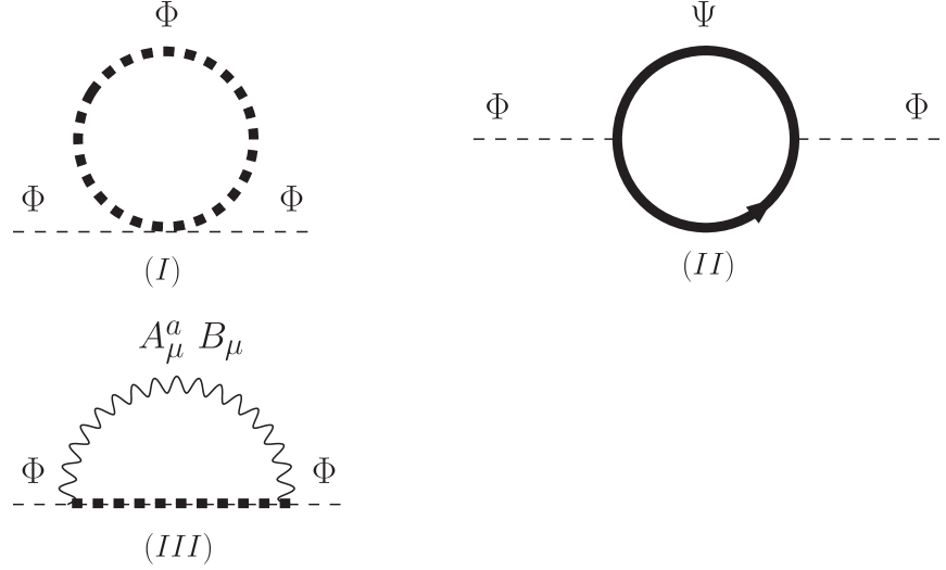
Figure 1: Self-energy Feynman diagrams for the Higgs bosons that contain loop particles affected by the hypermagnetic field. These particles are represented by thick lines. $\Phi$ and $\Psi$ represent Higgs and Fermion fields whereas $A_{\mu}^{a}$ and $B_{\mu}$ represent the $U(1)_{Y}$ and $SU(2)_{L}$ gauge fields, respectively.

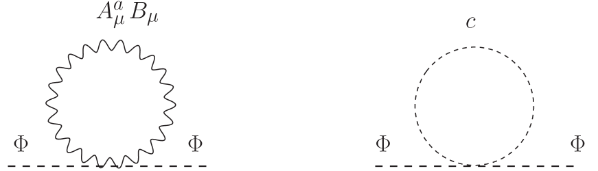
Figure 2: Self-energy Feynman diagrams for the Higgs bosons that contain loop particles not affected by the hypermagnetic field. These particles are represented by thin lines. $c$ represents the ghost fields. Working in the Landau gauge $\xi=0$, the second diagram vanishes.

In what follows, we work in the imaginary-time formalism of thermal field theory. First, we note that the integration over four-momenta is carried out in Euclidean space with $k_{0}=ik_{4}$, this means that

$$\int\frac{d^{4}k}{(2\pi)^{4}}\rightarrow i\int\frac{d^{4}k_{E}}{(2\pi)^{4}}.$$ (23)

Next, we recall that boson energies take discrete values, namely $k_{4}=\omega_{n}=2n\pi T$ with $n$ an integer, and thus

$$\int\frac{d^{4}k_{E}}{(2\pi)^{4}}\rightarrow T\sum_{n}\int\frac{d^{3}k}{(2\pi)^{3}}.$$ (24)

IV.1 Higgs boson

Figure 1 shows the diagrams that contribute to the Higgs boson self-energies affected by the hypermagnetic field. Let us explicitly compute the momentum independent diagram shown in fig. 1($I$) for a single scalar field. In the weak field limit, its expression is

$$\Pi^{Higgs}_{(I)} = \frac{\lambda}{4}T\sum_{n}\int\frac{d^{3}{\bf k}}{(2\pi)^{3}}$$ (25)

$$\times D_{H}(\omega_{n},{\bf k};m^{2}\rightarrow m^{2}+\Pi_{1}),$$

where $D_{H}$ is given by Eq. (11). Notice that Eq. (25) is computed self-consistently, with the approximation that on the right hand-side, $\Pi^{Higgs}_{(I)}\rightarrow\Pi_{1}$, where $\Pi_{1}$ is given by Carrington

$$\Pi_{1} = \frac{T^{2}}{4}\left\{\frac{3}{4}g^{2}+\frac{1}{4}g^{\prime 2}+2\lambda+f^{2}\right\},$$ (26)

and represents the leading temperature contribution to the scalar self-energy. The need to compute $\Pi^{Higgs}$ self-consistently is linked to the fact that, on the one hand, in the SM, scalar masses can vanish as a function of $v$ and, on the other, the presence of the magnetic field originates terms inversely proportional to these masses [see Eq. (34)]. Thus, for soft momentum, where the contribution of the ring diagrams is relevant, a naive perturbative expansion is not sufficient. The well known correction of the infrared behavior is given by the plasma screening properties and in the case of Eq. (25) we approximate such correction as consisting only of the leading temperature contribution to $\Pi^{Higgs}$ which, upon resummation, take care of the most severe infrared divergences Dolan .

Using the Euclidean version of Eq. (11), we have

$$\Pi^{Higgs}_{(I)} = \frac{\lambda}{4}T\sum_{n}\int\frac{d^{3}{\bf k}}{(2\pi)^{3}}\frac{1}{(\omega_{n}^{2}+{\bf k}^{2}+\tilde{m}^{2})}$$ (27)

$$\times \left(1-\frac{({\mbox{{\bf\scriptsize{Y}}}}H)^{2}}{(\omega_{n}^{2}+{\bf k}^{2}+\tilde{m}^{2})^{2}}\right.$$

$$+ \left.\frac{2({\mbox{{\bf\scriptsize{Y}}}}H)^{2}{\bf k}_{\perp}^{2}}{(\omega_{n}^{2}+{\bf k}^{2}+\tilde{m}^{2})^{3}}\right),$$

where we use the short hand notation $\tilde{m}^{2}=m^{2}+\Pi_{1}$.

The integrand in Eq. (27) contains terms whose general form is

$$I_{\alpha\beta}({\bf k},{\bf q})=\frac{1}{[\omega_{n}^{2}+{\bf k}^{2}+\tilde{m}^{2}]^{\alpha}[\omega_{n}^{2}+{({\bf k-q})}^{2}+\tilde{m}^{2}]^{\beta}}.$$

(28)

We make use of the Feynman parametrization to write $I_{\alpha\beta}$ as

$$I_{\alpha\beta}({\bf k},{\bf q})=\frac{\Gamma(\alpha+\beta)}{\Gamma(\alpha)\Gamma(\beta)}\int_{0}^{1}\frac{dx\ x^{\alpha-1}(1-x)^{\beta-1}}{[\omega_{n}^{2}+{\bf k^{\prime}}^{2}(x)+{m^{\prime}}^{2}(x)]^{\alpha+\beta}},$$

(29)

where

$${\bf k^{\prime}}(x) = {\bf k}-(1-x){\bf q}$$

$${m^{\prime}}^{2}(x) = \tilde{m}^{2}+x(1-x){\bf q}^{2},$$ (30)

and $\Gamma$ is the Gamma function. Notice that this parametrization is allowed since we work in the imaginary-time formalism weldon .

To carry out the sum over Matsubara frequencies together with the integration in Eq. (27), we perform an asymptotic expansion in the high temperature limit. This is done by means of a Mellin transform as described in detail in Ref. Bedingham . The explicit result, generalized to also include the fermion case is

$$T\sum_{n}\int\frac{d^{d}k}{(2\pi)^{d}}{\bf k}^{2a}{\omega^{2t}_{n}}I_{\alpha\beta}({\bf k},{\bf q}) = \frac{(2T)(2\pi T)^{d+2a+2t-2(\alpha+\beta)}}{(4\pi)^{d/2}\Gamma(\alpha)\Gamma(\beta)}\frac{\Gamma(\frac{d}{2}+a)}{\Gamma(\frac{d}{2})}\mu^{2\epsilon}\sum_{j=0}^{\infty}\frac{(-1)^{j}}{j!}\zeta(2(j+\alpha+\beta-t-\frac{d}{2}-a),Z)$$ (31)

$$\times \Gamma(j+\alpha+\beta-\frac{d}{2}-a)\int_{0}^{1}dx\ x^{\alpha-1}\ (1-x)^{\beta-1}\left(\frac{m^{\prime}(x)}{2\pi T}\right)^{2j},$$

where $\zeta$ is the modified Riemann Zeta function, $\mu$ is the energy scale of dimensional regularization and $d=3-2\epsilon$. For fermions the sum runs over all integers $n$ and $Z=1/2$, while for bosons the $n=0$ term is excluded and $Z=0$. It is important to stress that the method advocated in Ref. Bedingham to perform an expression such as Eq. (31) calls for the use of dimensional regularization, which is an appropriate method to use for non-Abelian gauge theories.

For the terms involving the $n=0$ Matsubara frequency for bosons, we use the result

$$T\int\frac{d^{d}k}{(2\pi^{d})}{\bf k}^{2a}I_{\alpha\beta}({\bf k},{\bf q}) = \frac{T}{(4\pi)^{d/2}}\frac{\Gamma(\frac{d}{2}+a)}{\Gamma(\frac{d}{2})}\frac{\Gamma(\alpha+\beta-\frac{d}{2})}{\Gamma(\alpha)\Gamma(\beta)}\int_{0}^{1}dx\ x^{\alpha-1}\ (1-x)^{\beta-1}\left(\frac{1}{m^{\prime}(x)}\right)^{2\alpha+2\beta-d+2a}.$$ (32)

In terms of the functions $I_{\alpha\beta}$ defined in Eq. (28) we can write Eq. (27) as

$$\Pi^{Higgs}_{(I)} = \frac{\lambda}{4}T\sum_{n}\int\frac{d^{3}{\bf k}}{(2\pi)^{3}}\Big{[}I_{10}({\bf k},0)+I_{30}({\bf k},0)$$ (33)

$$+ I_{40}({\bf k},0)\Big{]}.$$

Using Eq. (31) for the terms with $n\neq 0$ and Eq. (32) for the term with $n=0$, we get

$$\Pi^{Higgs}_{(I)}=\frac{\lambda}{2}T^{2}\left(1-\sum_{i=1}^{2}\left[\frac{3}{2\pi}\frac{\tilde{m}_{i}}{T}+\frac{({\mbox{{\bf\scriptsize{Y}}}}H)^{2}}{16\pi T\tilde{m}_{i}^{3}}\right]\right),$$ (34)

where we have included the contribution from all scalar fields with $\tilde{m}_{i}^{2}=m_{i}^{2}+\Pi_{1}$, $m_{i}$ standing for the scalar boson masses, given by

$$m_{1}^{2} = 3\lambda v^{2}-c^{2}$$

$$m_{2}^{2} = m^{2}_{3}=m_{4}^{2}=\lambda v^{2}-c^{2}.$$ (35)

In a similar fashion the contribution from the diagram in fig. 1($II$) in the infrared limit, namely $q_{0}=0$, $\mathbf{q}\rightarrow 0$, is

$$\Pi^{Higgs}_{(II)}(0)=\frac{f^{2}}{4}T^{2}\left(1+\frac{14\zeta(3)}{(2\pi)^{4}}\frac{({\mbox{{\bf\scriptsize{Y}}}}H)^{2}}{T^{4}}\right),$$ (36)

where hereafter we use the notation ${\mathcal{F}}(0)\equiv{\mathcal{F}}(q_{0}=0,{\bf q}\rightarrow 0)$ to represent the infrared limit of any function ${\mathcal{F}}$.

We point out that in Eqs. (34) and (36) we have kept terms representing the leading contribution of each kind arising in the calculation, namely, terms of order $({\mbox{{\bf\scriptsize{Y}}}}H)^{2}/T^{4}$, $\tilde{m}_{i}/T$ and $({\mbox{{\bf\scriptsize{Y}}}}H)^{2}/T\tilde{m}_{i}^{3}$. For the hierarchy of scales considered, the first kind of terms can be safely neglected. Recall that terms of order $\tilde{m}_{i}/T$ are usually neglected in a high temperature expansion. However, since we are here interested in keeping the leading contribution in the magnetic field strength, we are forced to keep this kind of terms which, for a large top quark mass, namely a large $f$, are of the same order as terms $({\mbox{{\bf\scriptsize{Y}}}}H)^{2}/T\tilde{m}_{i}^{3}$. Notice that for large values of the coupling constants, a perturbative calculation is not entirely justified. Nevertheless, here we consider our calculation as an analytical tool to explore this non-perturbative domain and regard terms of order $\tilde{m}_{i}/T$ as an estimate of the theoretical uncertainty of our results.

On the other hand, the diagram in fig. 1($III$) is proportional to the parameter $\xi$ and thus vanishes for our gauge parameter choice. Accounting also for the diagrams that are not affected by the hypermagnetic field, and that are depicted in fig. 2, the Higgs field self-energy, in the infrared limit is given by

$$\Pi^{Higgs}(0) = \frac{T^{2}}{4}\left\{\frac{3}{4}g^{2}+\frac{1}{4}g^{\prime 2}+2\lambda+f^{2}\right.$$ (37)

$$- \frac{\lambda}{\pi}\sum_{i=1}^{2}\left[\frac{3(m_{i}^{2}+\Pi_{1})^{1/2}}{T}\right.$$

$$+ \left.\left.\frac{({\mbox{{\bf\scriptsize{Y}}}}H)^{2}}{8T(m_{i}^{2}+\Pi_{1})^{3/2}}\right]\right\}.$$

IV.2 Gauge bosons

To express the gauge boson self-energies, in the presence of the external field, we have three independent vectors to our disposal to form tensor structures transverse to the gauge boson momentum $q^{\mu}$, namely $u^{\mu}$, $q^{\mu}$ and $b^{\mu}$. This means that in general, these self-energies can be written as linear combinations of nine independent structures Dolivo . Since we are interested in considering the infrared limit, $q_{0}=0,{\bf q}\rightarrow 0$, only $u^{\mu}$ and $b^{\mu}$ remain. Notice that the correct symmetry property for the self-energy is $\Pi_{ab}^{\mu\nu}(q)=\Pi_{ab}^{\nu\mu}(-q)$ nievespal . However, in the infrared limit, this condition means that the self-energy must be symmetric under the exchange of the Lorentz indices and therefore we can write.

$$\Pi^{\mu\nu}_{ab}=\Pi^{Q}_{ab}Q^{\mu\nu}+\Pi^{R}_{ab}R^{\mu\nu}+\Pi^{S}_{ab}S^{\mu\nu}+\Pi^{M}_{ab}g^{\mu\nu},$$ (38)

where

$$Q^{\mu\nu} = u^{\mu}u^{\nu},$$

$$R^{\mu\nu} = b^{\mu}b^{\nu},$$

$$S^{\mu\nu} = u^{\mu}b^{\nu}+u^{\nu}b^{\mu},$$ (39)

and the transversality condition $q_{\mu}\Pi^{\mu\nu}_{ab}=0$ is trivially satisfied in the infrared limit.

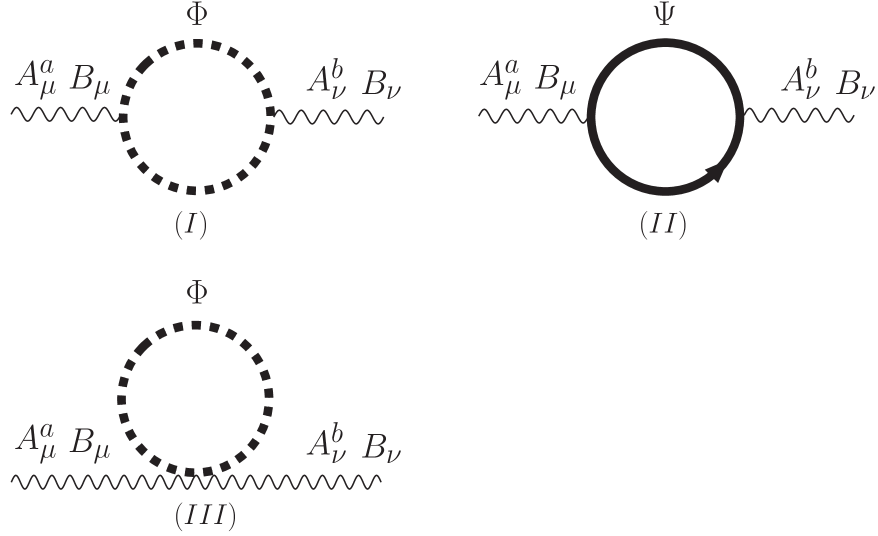
Figure 3: Self-energy Feynman diagrams for the gauge bosons that contain loop particles affected by the hypermagnetic field. These particles are represented by thick lines. $\Phi$ and $\Psi$ represent Higgs and Fermion fields whereas $A_{\mu}^{a}$ and $B_{\mu}$ represent the $U(1)_{Y}$ and $SU(2)_{L}$ gauge fields, respectively.

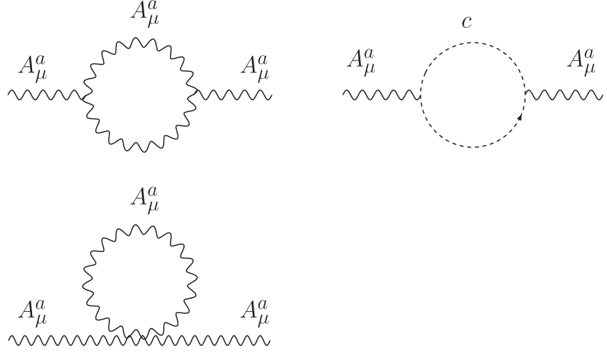
Figure 4: Self-energy Feynman diagrams for the gauge bosons that contain loop particles not affected by the hypermagnetic field. These particles are represented by thin lines. $c$ represents the ghost fields.

Figure 3 shows the gauge boson self-energy diagrams that are affected by the external hypermagnetic field. These include diagrams involving scalars as well as fermions in the loop. Let us explicitly compute the diagram shown in fig. 3($I$) for the $B_{\mu}$ field. Its expression is

$$\Pi^{\mu\nu}_{(I)B}(q) = \left(\frac{g^{\prime}}{2}\right)^{2}\int\frac{d^{4}k}{(2\pi)^{4}}(2k^{\mu}-q^{\mu})(2k^{\nu}-q^{\nu})$$ (40)

$$\times D_{H}(k)D_{H}(k-q).$$

Notice that since the net hypercharge flowing in the loop is zero, the phase factor in Eq. (3) vanishes.

Let us compute $\Pi^{00}_{(I)B}$ for a single scalar field with mass $m$. Working in the rest frame of the medium, $\Pi^{00}_{(I)B}=\Pi^{Q}_{(I)B}+\Pi^{M}_{(I)B}$. From Eq. (40) and at finite temperature this component is given by

$$\Pi^{00}_{(I)B}(q) = -g^{\prime 2}T\sum_{n}\int\frac{d^{3}k}{(2\pi)^{3}}\omega_{n}^{2}$$ (41)

$$\times D_{H}(\omega_{n},{\bf k};m^{2})$$

$$\times D_{H}(\omega_{n},{\bf k-q};m^{2}).$$

Since the integral in Eq. (41) does not give rise to terms inversely proportional to $m$, we have omitted the replacement $m^{2}\rightarrow m^{2}+\Pi_{1}$.

Using the Euclidean version of the scalar propagator $D_{H}$ obtained from Eq. (11), and in terms of the functions $I_{\alpha\beta}$ defined in Eq. (29), we can write Eq. (41) as

$$\Pi^{00}_{(I)B}(0)=-g^{\prime 2}T\sum_{n}\int\frac{d^{3}k}{(2\pi)^{3}}\omega_{n}^{2}\left\{I_{11}({\bf k},0)+({\mbox{{\bf\scriptsize{Y}}}}H)^{2}\left[I_{13}({\bf k},0)+I_{31}({\bf k},0)+2{\bf k}^{2}_{\perp}I_{14}({\bf k},0)+2{\bf k}^{2}_{\perp}I_{41}({\bf k},0)\right]\right\}.$$ (42)

Using Eq. (31) into Eq. (42) and keeping only the leading term as discussed in Sec. IV.1, we get

$$\Pi^{00}_{(I)B}(0) = \frac{g^{\prime 2}}{12}T^{2}$$ (43)

where the contribution from the four real scalar fields has been accounted for.

In a similar fashion, the explicit expressions for $\Pi^{00}_{(II)B}$ and $\Pi^{00}_{(III)B}$ are computed to yield

$$\Pi^{00}_{(II)B}(0) = \frac{5g^{\prime 2}}{3}T^{2}$$

$$\Pi^{00}_{(III)B}(0) = \frac{g^{\prime 2}}{12}T^{2}\left(1-\sum_{i=0}^{4}\left[\frac{3}{4\pi}\frac{\tilde{m}_{i}}{T}+\frac{1}{32\pi}\frac{({\mbox{{\bf\scriptsize{Y}}}}H)^{2}}{T\tilde{m}_{i}^{3}}\right]\right),$$

where in the first of the Eqs. (LABEL:auto1bcres) we have performed the sum over all hypercharged fermions. We stress that the origin of the terms $\sim 1/\tilde{m}_{i}^{3}$ is the topology of diagrams such as the one in fig. 3($III$) or fig. 1($I$), involving a tadpole of hypercharged scalars in the presence of the external field. In the computation of these diagrams, we require to consider the replacement $m^{2}\rightarrow m^{2}+\Pi_{1}$ (see the discussion in Sec. IV.1).

Adding up the above three contributions, we get

$$\Pi^{00}_{B}=\frac{11}{6}g^{\prime 2}T^{2}\left(1-\sum_{i=0}^{4}\left[\frac{3}{88\pi}\frac{\tilde{m}_{i}}{T}+\frac{1}{704\pi}\frac{({\mbox{{\bf\scriptsize{Y}}}}H)^{2}}{T\tilde{m}_{i}^{3}}\right]\right).$$

(45)

Performing a similar exercise for the case of the ${\bf A}_{\mu}$ fields, for which we also include the contribution from the diagrams that are not affected by the hypermagnetic field, depicted in fig. 4, we can write the result for the four gauge bosons as

$${\Pi^{00}_{ab}} = {\tilde{g}}^{2}\frac{11}{6}T^{2}\left(1-\sum_{i=0}^{4}\left[\frac{3}{88\pi}\frac{(m_{i}^{2}+\Pi_{1})^{1/2}}{T}\right.\right.$$ (46)

$$+ \left.\left.\frac{1}{704\pi}\frac{({\mbox{{\bf\scriptsize{Y}}}}H)^{2}}{T(m_{i}^{2}+\Pi_{1})^{3/2}}\right]\right)\delta_{ab}$$

$$\equiv \tilde{g}^{2}\Pi_{G}(T,H)\delta_{ab}.$$

where ${\tilde{g}}=g$ for a=b=1,2,3 and ${\tilde{g}}=g^{\prime}$ for a=b=4.

As is sketched in the appendix, the other non zero components of the gauge boson self-energy are negligible

$$\Pi^{11}_{ab}=\Pi^{22}_{ab},\ \Pi^{33}_{ab} \sim {\mathcal{O}}(m_{i}^{2})$$

$$\Pi^{03}_{ab}=\Pi^{30}_{ab} \sim {\mathcal{O}}({\mbox{{\bf\scriptsize{Y}}}}H),$$ (47)

which means that $\Pi^{00}_{ab}\simeq\Pi^{Q}_{ab}$.

Notice that in Eq. (46) we have not included terms of order ${\mathcal{O}}(M_{ab}/T)$, where $M_{ab}$ is the gauge boson mass matrix. These masses are proportional to $\tilde{g}v$ whereas for large $f$, $\tilde{m}_{i}$ are proportional to $fv$. Thus in this limit, terms of order ${\mathcal{O}}(M_{ab}/T)$ are smaller than terms of order ${\mathcal{O}}(\tilde{m}_{i}/T)$. These terms can in principle be calculated by diagonalization of $M_{ab}$ or else by explicitly considering the calculation in the basis of fields in the broken symmetry phase. We will present such calculation in a forthcoming work along with the gauge parameter dependence of the self-energies and effective potential.

Although in principle the fermion self-energies are also affected by the hypermagnetic field, as in the case of zero external field, their contribution to the ring diagrams is subdominant in the infrared and do not need to be taken into account.

V Effective Potential

V.1 One-loop

In the standard model the tree level potential is

$$V_{tree}(v)=-\frac{1}{2}c^{2}v^{2}+\frac{1}{4}\lambda v^{4}.$$ (48)

To one loop, the effective potential (EP) receives contributions from each sector, namely

$$V^{(1)}(v)=V^{(1)}_{gb}(v)+V^{(1)}_{Higgs}(v)+V^{(1)}_{f}(v),$$ (49)

where in general each one of these contributions is given by

$$V^{(1)}(v)=\frac{T}{2}\sum_{n}\int\frac{d^{3}k}{(2\pi)^{3}}{\mbox{Tr}}\left(\ln\left[D(\omega_{n},{\bf k})^{-1}\right]\right),$$ (50)

with $D$ stands for either the scalar, fermion or gauge boson propagator, and the trace is taken over all internal indices.

In the weak field limit, the contribution from the Higgs sector is given by

$$V^{(1)}_{Higgs} = \sum_{i=1}^{4}\frac{T}{2}\sum_{n}\int\frac{d^{3}k}{(2\pi)^{3}}\ln[D_{H}^{-1}(\omega_{n},{\bf k};m_{i}^{2}\rightarrow m_{i}^{2}+\Pi_{1})]\simeq\sum_{i=1}^{4}\frac{T}{2}\sum_{n}\int\frac{d^{3}k}{(2\pi)^{3}}\Big{\{}\ln(\omega_{n}^{2}+{\mathbf{k}}^{2}+m_{i}^{2}+\Pi_{1})$$ (51)

$$+ ({\mbox{{\bf\scriptsize{Y}}}}H)^{2}\left[\frac{1}{(\omega_{n}^{2}+{\mathbf{k}}^{2}+m_{i}^{2}+\Pi_{1})^{2}}-\frac{2(k_{\perp}^{2})}{(\omega_{n}^{2}+{\mathbf{k}}^{2}+m_{i}^{2}+\Pi_{1})^{3}}\right]\Big{\}}\,.$$

The first term in Eq. (51) with $\Pi_{1}=0$ represents the lowest order contribution to the effective potential at finite temperature and zero external magnetic field, usually referred to as the boson ideal gas contribution LeBellac . In order to keep track of the lowest order corrections in $\lambda$, we set $\Pi_{1}=0$ in Eq. (51). Thus for the hierarchy of scales considered here and dropping out the zero-point energy, this contribution is given by Dolan

$$\sum_{i=1}^{4}\frac{T}{2}\sum_{n}\int\frac{d^{3}k}{(2\pi)^{3}}\ln(\omega_{n}^{2}+{\mathbf{k}}^{2}+m_{i}^{2})\simeq\sum_{i=1}^{4}\left(-\frac{\pi^{2}T^{4}}{90}+\frac{m_{i}^{2}T^{2}}{24}-\frac{m_{i}^{3}T}{12\pi}-\frac{m_{i}^{4}}{32\pi^{2}}\ln\left(\frac{m_{i}}{4\pi T}\right)+{\mathcal{O}}(m_{i}^{4})\right).$$ (52)

Notice that there are potentially dangerous terms $m_{i}^{3}$ in Eq (52) that can become imaginary for negative values of $m_{i}$. However as we will show, these terms cancel when including the Higgs contribution from the ring diagrams.

The second, $H$-dependent term in Eq. (51) vanishes identically nosotros . Therefore, to one-loop order, the contribution to the EP in the weak field case from the Higgs sector is independent of ${\mbox{{\bf\scriptsize{Y}}}}H$ and is given by Eq. (52).

In the weak field limit, the contribution from the fermion sector is given by

$$V^{(1)}_{f}=\sum_{i=1}^{N_{f}}T\sum_{n}\int\frac{d^{3}k}{(2\pi)^{3}}\ln[S_{H}^{-1}(\omega_{n},{\bf k};{m_{f}}_{i})] \simeq \sum_{i=1}^{N_{f}}2T\sum_{n}\int\frac{d^{3}k}{(2\pi)^{3}}\Big{\{}\ln[\omega_{n}^{2}+{\bf k}^{2}+{m_{f}}_{i}^{2}]$$ (53)

$$+ 2({\mbox{{\bf\scriptsize{Y}}}}H)^{2}\frac{\omega_{n}^{2}+k_{3}^{2}+{m_{f}}_{i}^{2}}{(\omega_{n}^{2}+{\bf k}^{2}+{m_{f}}_{i}^{2})^{3}}\Big{\}},$$

where the sum runs over the number of SM fermions, $N_{f}$, with masses ${m_{f}}_{i}=\frac{f}{\sqrt{2}}v$. We emphasize that the only fermion mass we keep in the analysis is the top mass.

The first term in Eq. (53) represents the fermion ideal gas contribution LeBellac , which is explicitly given by Dolan

$$\sum_{i=1}^{N_{f}}2T\sum_{n}\int\frac{d^{3}k}{(2\pi)^{3}}\ln[\omega_{n}^{2}+{\bf k}^{2}+{m_{f}}_{i}^{2}] \simeq \sum_{i=1}^{N_{f}}\Big{\{}-7\frac{\pi^{2}T^{4}}{180}+\frac{{m_{f}}_{i}^{2}T^{2}}{12}+\frac{{m_{f}}_{i}^{4}}{16\pi^{2}}\ln\left(\frac{{m_{f}}_{i}^{2}}{T^{2}}\right)+{\mathcal{O}}({m_{f}}_{i}^{4})\Big{\}}.$$ (54)

The second term in Eq. (53) is subdominant, after taking care of renormalization and running of the coupling constant, as we sketch in the Appendix. Therefore, to one-loop order, the contribution to the EP in the weak field case from the fermion sector is only given by Eq. (54).

Finally, since in the symmetric phase the gauge bosons do not couple to the external field, their contribution to the EP is given by Carrington

$$V^{(1)}_{gb} = \sum_{G}\frac{T}{2}\sum_{n}\int\frac{d^{3}k}{(2\pi)^{3}}{\mbox{Tr}}\ln[{(D^{\mu\nu}_{ab})}^{-1}(\omega_{n},{\bf k};m_{G})]$$ (55)

$$\simeq \frac{T}{2}\sum_{n}\int\frac{d^{3}k}{(2\pi)^{3}}\Big{\{}6\ln(\omega_{n}^{2}+{\mathbf{k}}^{2}+m_{W}^{2})$$

$$+ \ 3\ln(\omega_{n}^{2}+{\mathbf{k}}^{2}+m_{Z}^{2})$$

$$+ 2\ln(\omega_{n}^{2}+{\mathbf{k}}^{2})\Big{\}},$$

where on the right-hand side in the first line, the index $G$ runs over the four SM gauge bosons and thereafter, we have used the mass eigenbasis with $m_{W}^{2}=g^{2}v^{2}/4$ and $m_{Z}^{2}=(g^{2}+g^{\prime 2})v^{2}/4$. The factors in front of each contribution correspond to the two $W^{\prime}$s, the $Z$ and the photon polarizations.

Using Eq. (52) into Eq. (55), the contribution to the EP from the gauge boson sector is

$$V^{(1)}_{gb}=-11\frac{\pi^{2}T^{4}}{90}+3\frac{(2m_{W}^{2}+m_{Z}^{2})T^{2}}{24}-\frac{(2m_{W}^{3}+m_{Z}^{3})T}{12\pi}-6\frac{m_{W}^{4}}{32\pi^{2}}\ln\left(\frac{m_{W}}{4\pi T}\right)-3\frac{m_{Z}^{4}}{32\pi^{2}}\ln\left(\frac{m_{Z}}{4\pi T}\right)+{\mathcal{O}}(m_{W}^{4}).$$ (56)

In our expressions for the 1-loop potential, ultraviolet divergences are absorbed by the standard renormalization procedure arnold .

V.2 Ring diagrams

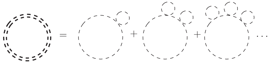
Figure 5: Schematic representation of ring diagrams, that consist in the resummation of successive insertions of self-energies in vacuum bubbles.

It is well known that the next order correction to the EP comes from the so called ring diagrams. These are schematically depicted in fig. 5. Their contribution to the EP is given by

$$V^{(ring)}_{Higgs}(v) = -\sum_{i=1}^{4}\frac{T}{2}\sum_{n}\int\frac{d^{3}k}{(2\pi)^{3}}\mbox{Tr}$$ (57)

$$\times \left\{\sum_{N=1}^{\infty}\frac{1}{N}\left[-D_{H}(\omega_{n},{\bf k};m_{i})\Pi^{Higgs}(0)\right]^{N}\right\}$$

$$= -\sum_{i=1}^{4}\frac{T}{2}\sum_{n}\int\frac{d^{3}k}{(2\pi)^{3}}$$

$$\times \mbox{Tr}\ \ln[1+\Pi^{Higgs}(0)D_{H}(\omega_{n},{\bf k};m_{i})],$$

for the scalar case, and by

$$V^{(ring)}_{gb}(v) = -\frac{T}{2}\sum_{n}\int\frac{d^{3}k}{(2\pi)^{3}}$$

$$\times \mbox{Tr}\left\{\sum_{N=1}^{\infty}\frac{1}{N}\left[-\Pi^{ab}_{\mu\lambda}(0)D_{bc}^{\lambda\nu}(\omega_{n},{\bf k})\right]^{N}\right\},$$

for the gauge boson case. The dominant contribution comes from the mode $n=0$ in Eqs. (57) and (LABEL:ringgb) LeBellac . The scalar case has been treated in detail in Ref. nosotros for the weak field limit and here we just quote the result

$$V^{(ring)}_{Higgs}\!\!=\!\!-\sum_{i=1}^{4}\left\{\frac{T}{12\pi}\left[\left(m_{i}^{2}+\Pi_{1}\right)^{3/2}-m_{i}^{3}\right]-\frac{({\mbox{{\bf\scriptsize{Y}}}}H)^{2}}{4\pi}\left(\frac{\Pi_{1}}{48}\right)\left(\frac{T}{(m_{i}^{2}+\Pi_{1})^{3/2}}\right)\right\},$$ (59)

where the contributions from all scalars has been accounted for.

In order to compute the contribution from the gauge bosons, we have to diagonalize the matrix product $\Pi^{ab}_{\mu\lambda}(0)D_{bc}^{\lambda\nu}(\omega_{n},{\bf k})$ in Eq. (LABEL:ringgb). In the gauge group space, we notice that since $\Pi^{ab}(0)$ is, according to Eq. (46), diagonal we can use the same matrix that diagonalizes the mass matrix, given explicitly for instance in Ref. arnold . On the other hand in Lorentz space, the Euclidean version of the gauge boson propagator in the Landau gauge can be written as

$$D_{\mu\nu} = \Big{\{}P^{L}_{\mu\nu}+P^{T}_{\mu\nu}\Big{\}}\frac{1}{k^{2}+m^{2}},$$ (60)

where

$$P^{T}_{00}=P^{T}_{0i}=0 P^{T}_{ij}=\delta_{ij}-{\bf\hat{k}}_{i}{\bf\hat{k}}_{j}$$

$$P^{L}_{\mu\nu}=\delta^{\mu\nu}\!\! - \!\!\frac{k_{\mu}k_{\nu}}{k^{2}}-P^{T}_{\mu\nu}.$$ (61)

It is easy to see that considering only the dominant term in the product $\Pi_{\mu\lambda}(0)D^{\lambda\nu}(\omega_{n},{\bf k})$ one gets

$$\Pi_{\mu_{\lambda}}D^{\lambda\nu} = \frac{\Pi^{Q}_{ab}}{k^{2}+m^{2}}\left[1+\frac{(k\cdot u)^{2}}{k^{2}}\right]Q_{\mu}^{\nu}.$$ (62)

Considering the $n=0$ term and taking the trace, Eq. (LABEL:ringgb) gives

$$V^{(ring)}_{gb}(v) = -\sum_{G}\frac{1}{2}T\int\frac{d^{3}k}{(2\pi)^{3}}\ln[1+\frac{\Pi^{Q}_{ab}}{{\bf k}^{2}+m_{G}^{2}}]$$ (63)

$$= -\frac{T}{12\pi}\left\{2m_{W}^{3}(T,H)+m_{Z}^{3}(T,H)+m_{\gamma}^{3}(T,H)-2m_{W}^{3}-m_{Z}^{3}\right\},$$

where $m_{G}(T,H)$ are explicitly given by

$$m_{W}^{2}(T,H) = m_{W}^{2}+g^{2}\Pi_{G}$$

$$m_{Z}^{2}(T,H) = \frac{1}{2}\left\{m_{Z}^{2}+(g^{2}+g^{\prime 2})\Pi_{G}+\sqrt{[m_{Z}^{2}+(g^{2}+g^{\prime 2})\Pi_{G}]^{2}-8\frac{g^{2}g^{\prime 2}\Pi_{G}}{(g^{2}+g^{\prime 2})}[m_{Z}^{2}+\frac{(g^{2}+g^{\prime 2})}{2}\Pi_{G}]}\right\}$$

$$m_{\gamma}^{2}(T,H) = \frac{1}{2}\left\{m_{Z}^{2}+(g^{2}+g^{\prime 2})\Pi_{G}-\sqrt{[m_{Z}^{2}+(g^{2}+g^{\prime 2})\Pi_{G}]^{2}-8\frac{g^{2}g^{\prime 2}\Pi_{G}}{(g^{2}+g^{\prime 2})}[m_{Z}^{2}+\frac{(g^{2}+g^{\prime 2})}{2}\Pi_{G}]}\right\}.$$

Note that both the temperature as well as the magnetic field corrections to the gauge boson masses are encoded in $\Pi_{G}$. When $H\rightarrow 0$ the gauge boson masses tend to their usual thermal masses Carrington

$$m_{W}^{2}(T,H\rightarrow 0) \rightarrow m_{W}^{2}(T)$$

$$m_{Z}^{2}(T,H\rightarrow 0) \rightarrow m_{Z}^{2}(T)$$

$$m_{\gamma}^{2}(T,H\rightarrow 0) \rightarrow m_{\gamma}^{2}(T).$$ (65)

where $m_{G}^{2}(T)$ can be obtained from Eqs. (46) and (LABEL:massT) by setting $H=0$.

To bring about the explicit dependence of $V_{gb}^{(ring)}$ on the hypermagnetic field strength, let us expand the the cube of the gauge boson masses appearing in Eq. (63) up to order $({\mbox{{\bf\scriptsize{Y}}}}H)^{2}$, which is our working order. From the expressions in Eqs. (LABEL:massT) this gives

$$V^{(ring)}_{gb}(v) = -\frac{T}{12\pi}\left\{2m_{W}^{3}(T)+m_{Z}^{3}(T)+m_{\gamma}^{3}(T)-2m_{W}^{3}-m_{Z}^{3}\right\}$$ (66)

$$+ \frac{T}{12\pi}\Big{\{}\frac{3}{4}\left[2g^{2}m_{W}(T)+(g^{2}+g^{\prime 2})(m_{Z}(T)R_{Z}-m_{\gamma}(T)R_{\gamma})\right]$$

$$\times \frac{T}{384\pi}\sum_{i=1}^{4}\left(\frac{1}{\left(m_{i}^{2}+\Pi_{1}\right)^{3/2}}\right)\Big{\}}({\mbox{{\bf\scriptsize{Y}}}}H)^{2}$$

where

$$R_{Z} = \frac{2m_{Z}^{2}(T)}{m_{Z}^{2}(T)-m_{\gamma}^{2}(T)}-\frac{g^{2}g^{\prime 2}}{(g^{2}+g^{\prime 2})^{2}}\frac{m_{Z}^{2}(T)+m_{\gamma}^{2}(T)}{m_{Z}^{2}(T)-m_{\gamma}^{2}(T)}$$

$$R_{\gamma} = \frac{2m_{\gamma}^{2}(T)}{m_{Z}^{2}(T)-m_{\gamma}^{2}(T)}-\frac{g^{2}g^{\prime 2}}{(g^{2}+g^{\prime 2})^{2}}\frac{m_{Z}^{2}(T)+m_{\gamma}^{2}(T)}{m_{Z}^{2}(T)-m_{\gamma}^{2}(T)}.$$

The final expression for the effective potential is obtained by adding up the results in Eqs. (48), (52), (54), (56), (59) and (66).

$$V(v) = V_{tree}(v)+V^{(1)}_{Higgs}+V_{f}^{(1)}+V^{(1)}_{gb}$$ (68)

$$+ V^{(ring)}_{Higgs}+V^{(ring)}_{gb}$$

Notice that the dangerous terms $m_{i}^{3}$ which come from $V^{(1)}_{Higgs}$ cancel with the corresponding terms coming from $V^{(ring)}_{Higgs}$. The cubic term in the masses of the gauge bosons do not cancel but since these masses are positive definite, these terms do not pose any problem. Also, in order for the terms involving the square of the bosons’ thermal mass to be real, the temperature must be such that

$$T>T_{1} \equiv \sqrt{\frac{-16m_{1}^{2}(v=0)}{3g^{2}+g^{\prime 2}+8\lambda+4f^{2}}},$$ (69)

which defines a lower bound for the temperature. A more restrictive bound is obtained by requiring that ${\mbox{{\bf\scriptsize{Y}}}}H<\tilde{m}^{2}$ for the weak field expansion to work. This condition translates into the bound

$$T>T_{2} \equiv \sqrt{\frac{{\mbox{{\bf\scriptsize{Y}}}}H-16m_{1}^{2}(v=0)}{3g^{2}+g^{\prime 2}+8\lambda+4f^{2}}}.$$ (70)

The relevant factor that enhances the order of transition, present both in $V^{(ring)}_{Higgs}$ and $V^{(ring)}_{gb}$, is $({\mbox{{\bf\scriptsize{Y}}}}H)^{2}/\tilde{m}_{i}^{3}$ which can be traced back to the boson self-energy diagrams involving a tadpole of hypercharged scalars in the presence of the external field.

VI Symmetry Breaking

In order to quantitatively check the effect of the magnetic field during the EWPT, we proceed to plot $V_{eff}$ as a function of the vacuum expectation value $v$. For the analysis we use $g^{\prime}=0.344$ and $g=0.637$, $m_{Z}=91$ GeV, $m_{W}=80$ GeV, $f=1$, $\lambda=0.11$ which corresponds to the current bound on the Higgs mass.

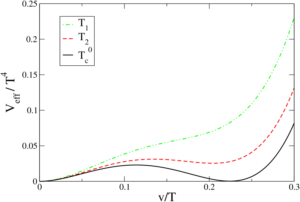
Figure 6: (Color on line) $V_{eff}$ as a function of $v$ for different temperatures and $H=0$. At high temperature ($T_{1}$) the symmetry is restored. Decreasing the temperature ($T_{2}$) causes $V_{eff}$ to develop a secondary minimum that becomes degenerate with the original one for a critical temperature $T_{c}^{0}<T_{1}<T_{2}$, where $v=v^{0}$. Lowering further the temperature below $T_{c}^{0}$ produces the system to spinodaly decompose. For the analysis we use $g^{\prime}=0.344$ and $g=0.637$, $m_{Z}=91$ GeV, $m_{W}=80$ GeV, $f=1$, $\lambda=0.11$.

Figure 6 shows $V_{eff}$ for different temperatures and $H=0$. This figure shows the usual behavior whereby at high temperature the symmetry is restored and, when decreasing the temperature, $V_{eff}$ develops a secondary minimum that becomes degenerate with the original one for a critical temperature $T_{c}^{0}$, where $v=v^{0}$. Lowering further the temperature below $T_{c}^{0}$ produces the system to spinodaly decompose.

To study the effect of the hypermagnetic field on the effective potential, we parametrize $H=h\,(100\ \mbox{GeV})^{2}$. In what follows, we always choose values for $h$ that comply with the condition $h({\mbox{{\bf\scriptsize{Y}}}}\,(100\ \mbox{GeV})^{2})<\tilde{m}_{1}^{2}(v=0)$, as required from our hierarchy of scales, since the smallest possible mass is always that of a scalar boson in the symmetric phase. Figure 7 shows $V_{eff}$ for different field strengths $H_{3}>H_{2}>H_{1}$ and constant $T$ where $T$ is taken as the critical temperature for the $h=0$ case. We can see that for higher field strengths, the phase transition is delayed, favoring higher values of the ratio of the vacuum expectation value $\langle v\rangle$ in the broken symmetry phase to the critical temperature $T_{c}$. This makes the transition stronger first order as the strength of the field increases.

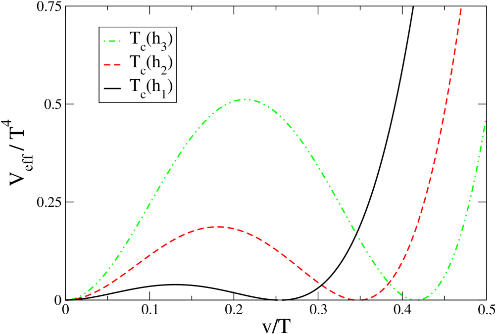
Figure 8: (Color on line) $V_{eff}$ as a function of $v$ for different hypermagnetic field strengths $h_{3}>h_{2}>h_{1}$ at their corresponding critical temperatures $T_{c}(h_{3})<T_{c}(h_{2})<T_{c}(h_{1})$, where $H=h\,(100\ \mbox{GeV})^{2}$. We note that increasing the intensity of the field, the barrier between minima becomes higher and that the ratio $\langle v\rangle/T$ becomes larger. For the analysis we use $g^{\prime}=0.344$ and $g=0.637$, $m_{Z}=91$ GeV, $m_{W}=80$ GeV, $f=1$, $\lambda=0.11$.

Figure 8 shows a comparison of $V_{eff}$ for different field strengths $H_{3}>H_{2}>H_{1}$ at their corresponding critical temperatures with $T_{c}(h_{3})<T_{c}(h_{2})<T_{c}(h_{1})$ for $h_{3}=0.25$, $h_{2}=0.2$ and $h_{1}=0.1$. From this figure we also note that increasing the intensity of the field, the barrier between minima becomes higher and the ratio $\langle v\rangle/T$ becomes larger, making the EWPT become stronger first order Petropoulos .

The effect of the hypermagnetic field is therefore twofold: first it delays the beginning of the phase transition and second the Higgs vacuum expectation value in the broken symmetry phase becomes larger. Both effects favor the suppression of the sphaleron transition rate and therefore help the freezing of a possible baryon asymmetry during the EWPT.

VII Discussion and Conclusions

In conclusion, we have shown that in the presence of an external magnetic field, the EWPT becomes stronger first order. Our treatment has been implemented for the case of weak fields for the hierarchy of scales ${\mbox{{\bf\scriptsize{Y}}}}H\ll m^{2}\ll T^{2}$ where $m$ is taken as a generic mass involved in the calculation. Notice that when this relation is applied to the case of the scalar masses, $m^{2}$ should be regarded as $\tilde{m}^{2}$. We have explicitly worked with the degrees of freedom in the symmetric phase where the external magnetic field belongs to the $U(1)_{Y}$ group and therefore properly receives the name of hypermagnetic field. The calculation is carried out up to the contribution of ring diagrams to the effective potential at finite temperature. To include the effects of this external field, we have made use of the Schwinger proper-time method. In this way, the contribution from all Landau levels has been accounted for. We have carried out a systematic expansion up to order $({\mbox{{\bf\scriptsize{Y}}}}H)^{2}$. The presence of the external hypermagnetic field gives rise to terms in the effective potential proportional to $1/\tilde{m}_{i}^{3}$, where $\tilde{m}_{i}^{2}=m_{i}^{2}+\Pi_{1}$, coming from tadpole diagrams in the boson self-energies where the loop particle is a hypercharged scalar and $m_{i}$ are their masses. These terms are the relevant ones for the strengthening of the order of the phase transition since $\tilde{m}_{i}(v)$ is small for small values of $v$, which enhances the curvature of the effective potential near $v=0$.

The presence of the hypermagnetic field has two simultaneous effects: first it delays the beginning of the phase transition as compared to the case with no hypermagnetic field. Second, the Higgs vacuum expectation value in the broken symmetry phase becomes larger. Both effects favor the suppression of the sphaleron transition rate and therefore help the freezing of a possible baryon asymmetry during the EWPT. Although our study suggests that for reasonable values of the magnetic field strength the ratio $\langle v\rangle/T$ does not reach the necessary values to avoid the sphaleron erasure, we should keep in mind that we have worked under very restrictive assumptions, derived from our assumed hierarchy of scales. Lifting some of the restrictions, in particular the weakness of the magnetic field compared to the mass scale, could open a window to make the above ratio larger, while remaining within the observational bounds. This is a subject under current study and will be reported elsewhere.

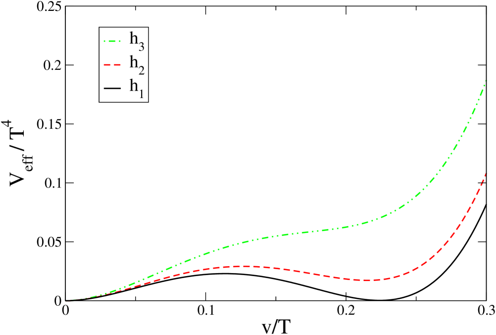
Figure 7: (Color on line) $V_{eff}$ as a function of $v$ for constant $T$ and different values $H=h\,(100\ \mbox{GeV})^{2}$ where $h_{1}=0$, $h_{2}=0.03$ and $h_{3}=0.06$. The choosen temperature $T$ is the critical temperature for $h_{1}=0$. For higher field strengths, the phase transition is delayed, favoring higher values of $\langle v\rangle/T_{c}$. For the analysis we use $g^{\prime}=0.344$ and $g=0.637$, $m_{Z}=91$ GeV, $m_{W}=80$ GeV, $f=1$, $\lambda=0.11$.

The calculation has been carried out in the framework of perturbation theory but in order to make contact with the values for the masses of the top quark and the current bounds on the Higgs mass, in the numerical analysis we have used large values for the coupling constants, in particular we have considered the top Yukawa coupling $f=1$. In this sense, our calculation has to be considered as an analytical tool to explore this non perturbative regime.

Our results go along the same direction as the ones obtained at tree Giovannini and one-loop Elmfors levels. We should however point out that the same problem has been also treated in Refs. Skalozub1 ; Skalozub2 in the context of strong external magnetic/hypermagnetic fields. These authors conclude that the magnetic field gives rise to logarithmic terms of the ratio of the temperature to the fermion masses and that for light fermions, these terms increase the inertia of the Higgs field producing the phase transition to become second order. Similar logarithmic terms appear in a weak field expansion of the effective potential in Ref. Persson although, as pointed out by the authors of that work, their weak field expansion is not necessarily reliable since it is given in terms of a Borel summable rather than a convergent series. In this work we have not come across such terms but a detailed comparison between the methods used in the above mentioned works with ours to include the effects of the magnetic field is certainly called for. Also the study of the gauge parameter dependence and the inclusion of small but not necessarily negligible terms proportional to the gauge boson masses is a natural extension of this work. Progress in this direction is being made and we will report on it elsewhere Jorge .

Appendix

First we sketch the computation of the diagram depicted in fig. 3($II$) representing the fermion contribution to the one-loop gauge boson self-energy tensor up to order $({\mbox{{\bf\scriptsize{Y}}}}H)^{2}$, where it is not evident that the off-diagonal components are negligible. We use the notation ${}^{n}\Pi_{\mu\nu}$, $n=0,1,2$, where $n$ is the power of ${\mbox{{\bf\scriptsize{Y}}}}H$. To zeroth order we have

$${}^{0}\Pi_{\mu\nu} = \left(\frac{g}{4}\right)^{2}T\sum_{n}\int\frac{d^{3}k}{(2\pi)^{3}}$$ (71)

$$\times \frac{16k_{\mu}k_{\nu}-8k^{2}\delta_{\mu\nu}}{[k^{2}+{m_{f}}_{i}^{2}][(k-p)^{2}+{m_{f}}_{i}^{2}]}.$$

Using the result in Eq. (31) for fermions we get

$${}^{0}\Pi_{\mu\nu} = \left(\frac{g}{4}\right)^{2}\Big{\{}\left(\frac{2}{3}T^{2}+\frac{{m_{f}}_{i}^{2}}{2\pi^{2}}\left[\frac{1}{\epsilon}+\gamma_{E}+\ln{\frac{4\mu^{2}}{\pi T^{2}}}-1\right]\right)$$

$$\times \delta_{\mu 0}\delta_{\nu 0}+\frac{{m_{f}}_{i}^{2}}{(4\pi)^{2}}\left[\frac{2}{3}+\frac{1}{\epsilon}+\gamma_{E}+\ln{\frac{4\mu^{2}}{\pi T^{2}}}\right]\delta_{i\mu}\delta_{j\nu}\Big{\}}\!.$$

To first order we have

$${}^{1}\Pi_{\mu\nu} = -8({\mbox{{\bf\scriptsize{Y}}}}H)\left(\frac{g}{4}\right)^{2}T\sum_{n}\int\frac{d^{3}k}{(2\pi)^{3}}$$ (73)

$$\times \left[k_{3}(k_{\mu}u_{\nu}+k_{\nu}u_{\mu})+\omega_{n}(k_{\mu}b_{\nu}+k_{\nu}b_{\mu})\right.$$

$$- \left.2\omega_{n}k_{3}\delta_{\mu\nu}\right][I_{12}({\bf k},{\bf q})+I_{21}({\bf k},{\bf q})]$$

$$+ 8i\epsilon_{\mu\nu\alpha\beta}\left[k_{3}k^{\alpha}u^{\beta}+\omega_{n}k^{\alpha}b^{\beta}\right]$$

$$\times [I_{12}({\bf k},{\bf q})-I_{21}({\bf k},{\bf q})].$$

Using again Eq. (31) we explicitly get

$${}^{1}\Pi_{\mu\nu} = \left(\frac{g}{4}\right)^{2}\frac{({\mbox{{\bf\scriptsize{Y}}}}H)}{2\pi^{2}}\left[\frac{1}{\epsilon}+\gamma_{E}+\ln{\frac{4\mu}{\pi T}}+\frac{1}{3}\right]$$ (74)

$$\times (\delta_{\mu 3}\delta_{\nu 0}+\delta_{\mu 0}\delta_{\nu 3}).$$

To second order we get contributions from two terms

$${}^{2}\Pi_{\mu\nu}^{a} = 8({\mbox{{\bf\scriptsize{Y}}}}H)^{2}\left(\frac{g}{4}\right)^{2}T\sum_{n}\int\frac{d^{3}k}{(2\pi)^{3}}\left[k_{3}^{2}(2u_{\mu}u_{\nu}-\delta_{\mu\nu})\right.$$ (75)

$$+ \left.2\omega_{n}k_{3}(u_{\mu}b_{\nu}+u_{\nu}b_{\mu})+\omega_{n}^{2}(2b_{\mu}b_{\nu}-\delta_{\mu\nu})\right]$$

$$\times I_{22}({\bf k},{\bf q}),$$

and

$${}^{2}\Pi_{\mu\nu}^{b} = -8({\mbox{{\bf\scriptsize{Y}}}}H)^{2}\left(\frac{g}{4}\right)^{2}T\sum_{n}\int\frac{d^{3}k}{(2\pi)^{3}}$$ (76)

$$\times \left[4k_{\mu}k_{\nu}(k_{3}^{2}-\omega_{n}^{2})-2((k_{\mu}b_{\nu}+k_{\nu}b_{\mu})k_{3}\right.$$

$$- \left.(k_{\mu}b_{\nu}+k_{\nu}b_{\mu})\omega_{n})(\omega_{n}^{2}+{\bf k}^{2})\right]$$

$$\times \left(I_{41}({\bf k},{\bf q})+I_{14}({\bf k},{\bf q})\right)$$

$$- 2i\epsilon_{\mu\nu\alpha\beta}\left[k_{3}b^{\alpha}k^{\beta}-\omega_{n}u^{\alpha}k^{\beta}\right]k^{2}$$

$$\times (I_{41}({\bf k},{\bf q})-I_{14}({\bf k},{\bf q})).$$

Using once more Eq. (31) we get

$${}^{2}\Pi_{\mu\nu}^{a} = -8\left(\frac{{\mbox{{\bf\scriptsize{Y}}}}H}{T}\right)^{2}\left(\frac{g}{4}\right)^{2}\frac{7\xi(3)}{48\pi^{4}}\left\{\delta_{\mu 0}\delta_{\nu 0}\right.$$ (77)

$$+ \left.(2+3b^{i}b^{j})\delta_{\mu i}\delta_{\nu j}\right\},$$

and

$${}^{2}\Pi_{\mu\nu}^{b} = 8\left(\frac{{\mbox{{\bf\scriptsize{Y}}}}H}{T}\right)^{2}\left(\frac{g}{4}\right)^{2}\frac{7\xi(3)}{144\pi^{4}}\left\{\delta_{\mu i}\delta_{\nu j}\right.$$ (78)

$$+ \left.6\delta_{\mu 3}\delta_{\nu 3}-9\delta_{\mu 0}\delta_{\nu 0}\right\}.$$

From Eq. (LABEL:A1a), we see that the leading contribution corresponds to the term proportional to $T^{2}$ and thus the result in the first of Eqs. (LABEL:auto1bcres), after summing over all hypercharged fermions. After factorizing the leading contribution, we also notice that the terms proportional to $({m_{f}}_{i}/T)^{2}$ come together with a factor reminiscent of renormalization and running of the fermion mass and couplings with the scale $\mu$. We do not carry out this procedure in detail but when absorbing these factors into the redefinition of the fermion mass, we see that corrections to the leading term are proportional to $({m_{f}}_{i}/T)^{2}$ and therefore for the values taken by $v$ during the EWPT, these corrections can be safely neglected.

From Eq. (74), and by the same procedure as for the case of the zeroth order terms, the off-diagonal terms contribute an amount proportional to ${\mbox{{\bf\scriptsize{Y}}}}H/T^{2}$, compared to the leading term and thus for the hierarchy of scales considered, this term can also be neglected.

Finally from Eqs. (77) and (78) we can see that the second order contributions are proportional to $({\mbox{{\bf\scriptsize{Y}}}}H/T^{2})^{2}$ and therefore can also be safely neglected.

Next, we sketch the computation of the hypermagnetic field contribution to the fermion one-loop effective potential $V_{f}^{(1)}$. According to Eq. (53), this contribution is of second order in ${\mbox{{\bf\scriptsize{Y}}}}H$.

$${}^{2}V_{f}^{(1)}=2({\mbox{{\bf\scriptsize{Y}}}}H)^{2}T\sum_{n}\int\frac{d^{3}k}{(2\pi)^{3}}\frac{\omega_{n}^{2}+k_{3}^{2}+{m_{f}}_{i}^{2}}{(\omega_{n}^{2}+{\bf k}^{2}+{m_{f}}_{i}^{2})^{3}}.$$ (79)

Using Eq. (31) we get

$${}^{2}V_{f}^{(1)} = \frac{2({\mbox{{\bf\scriptsize{Y}}}}H)^{2}}{32\pi^{2}}\left[\frac{1}{\epsilon}-\frac{7\xi(3)}{2\pi^{2}}\frac{{m_{f}}_{i}^{2}}{T^{2}}\right.$$ (80)

$$+ \left.\ln(\frac{4\mu^{2}}{\pi T^{2}})+\gamma_{E}+\frac{2}{3}\right].$$

After renormalization and running of the couplings with the scale $\mu$ we see that this contribution is of order $({\mbox{{\bf\scriptsize{Y}}}}H/T^{2})^{2}$ and can also be safely neglected.

References

- (1) A.D. Sakharov, Pis’ma Zh. Éksp. Teor. Fiz. 5, 32 (1967) [JETP Lett. 5, 24 (1967)].
- (2) M.B. Gavela, P. Hernández, J. Orloff and O. Pène, Mod. Phys. Lett. A 9, 795 (1994).
- (3) K. Kajantie, M. Laine, K. Rummukainen and M. Shaposhnikov, Nucl. Phys. B466, 189 (1996).
- (4) F.R. Klinkhamer and N.S. Manton, Phys. Rev. D30, 2212 (1984).
- (5) For comprehensive reviews on EW baryogenesis see for example: M. Trodden, Rev. Mod. Phys. 71, 1463 (1999); A. Megevand, Int. J. Mod. Phys. D 9, 733 (2000).
- (6) N. Petropoulos, “Baryogenesis at the electroweak phase transition”, hep-ph/0304275.
- (7) For comprehensive reviews see P.P. Kronberg, Rep. Prog. Phys. 57, 325 (1994); R. Beck, A. Brandedenburg, D. Moss, A. Shukurov and D. Sokoloff, Annu. Rev. Astron. Astrophysics, 34, 155 (1996); C.L. Carilli and G.B. Taylor, Ann. Rev. Astron. Astrophysics, 40, 319 (2002).
- (8) J.D. Barrow, P. Ferreira and J. Silk, Phys. Rev. Lett. 78, 3610 (1997).
- (9) D.G. Yamazaki, K. Ichiki, T. Kajino and G.J. Mathews, Constraints on the evolution of the primordial magnetic field from the small scale cmb angular anisotropy, astro-ph/0602224.
- (10) See J.D. Barrow, R. Maartens and C.G. Tsagas, Cosmology with inhomogeneous magnetic fields, astro-ph/0611537 and references therein.
- (11) D. Grasso and H.R. Rubinstein, Phys. Lett. 379 73, (1996)
- (12) See for example: G. Piccinelli and A. Ayala, Lect. Notes Phys. 646, 293-308 (2004).
- (13) M. Giovannini and M. E. Shaposhnikov, Phys. Rev. D57, 2186 (1998).
- (14) P. Elmfors, K. Enqvist and K. Kainulainen, Phys. Lett. B 440, 269 (1998).
- (15) K. Kajantie, M. Laine, J. Peisa, K. Rummukainen and M. Shaposhnikov, Nucl. Phys. B 544, 357 (1999).
- (16) A. Ayala, J. Besprosvany, G. Pallares and G. Piccinelli, Phys. Rev. D64, 123529 (2001); A. Ayala, G. Piccinelli and G. Pallares, Phys. Rev. D66, 103503 (2002), A. Ayala and J. Besprosvany, Nucl. Phys. B651, 211 (2004).
- (17) D. Comelli, D. Grasso, M. Pietroni and A. Riotto, Phys. Lett. B458, 304 (1999).
- (18) V. Skalozub and V. Demchik, Electroweak phase transition in strong magnetic fields in the Standard Model of elementary particles; hep-th/9912071.
- (19) V. Skalozub and M. Bordag, Int. J. Mod. Phys. A 15, 349 (2000).
- (20) M.E. Carrington, Phys. Rev. D45, 2933 (1992).
- (21) J. Schwinger, Phys. Rev. 82, 664 (1951).
- (22) A. Ayala, A. Sánchez, G. Piccinelli and S. Sahu, Phys. Rev. D71, 023004 (2005).
- (23) T.-K. Chyi, C.-W. Hwang, W.F. Kao, G.L. Lin, K.-W. Ng and J.-J. Tseng, Phys. Rev. D 62, 105014, (2000).
- (24) R. Maartens, Pramana 55, 575 (2000).
- (25) J. Ambjørn and P. Olesen, Nucl. Phys. B315, 606 (1989).
- (26) L. Dolan and R. Jackiw, Phys. Rev. D9, 3320 (1974).
- (27) N. K. Nielsen, Nucl. Phys. B 101, 173 (1975).
- (28) M. Le Bellac Thermal Field Theory, Cambridge University Press (1996).
- (29) H.A. Weldon, Phys. Rev. D47, 594 (1993).
- (30) D.J. Bedingham, “Dimensional regularization and Mellin summation in high temperature calculations”, hep-ph/0011012.
- (31) J.C. D’Olivo, J.F. Nieves, S. Sahu, Phys. Rev. D 67, 025018 (2003).
- (32) J.F. Nieves and P.B. Pal, Phys. Rev. D39, 652 (1989).
- (33) P. Arnold and O. Espinosa Phys. Rev. D47, 3546 (1993).
- (34) P. Elmfors, D. Persson and B.-S. Skagerstam, Astropart. Phys. 2 299 (1994).
- (35) J.L. Navarro, A. Ayala, G. Piccinelli, A. Sánchez and M.E. Tejeda, in progress.