A proposal for detecting second order topological quantum phase

Abstract

Gaussian linking of a semiclassical path of a charged particle with a magnetic flux tube is responsible for the Aharonov-Bohm effect, where one observes interference proportional to the magnitude of the enclosed flux. We construct quantum mechanical wave functions where semiclassical paths can have second order linking to two magnetic flux tubes, and show there is interference proportional to the product of the two fluxes.

Topological phases can arise when a particle traverses semiclassical paths that cannot be deformed into each other due to some obstruction in an experimental setup, for example, paths that pass on opposite sides of an infinitely long solenoid. If the particle is charged, and there is a magnetic flux confined within the obstruction, then the two paths experience different vector potentials. This generates a phase difference for the two topologically different paths and causes interference when the particle is detected. The magnitude of the phase is a measure of the Gaussian linking of the particle path with the solenoid. What we have described here is the Aharonov-Bohm effect Aharonov:1959fk . But, this is not the full story, as we will now argue.

Higher order linking is possible. Consider the Borromean rings, an arrangement of three loops inextricably linked Rolfsen but with no first order (Gaussian) linking between any pair (see Fig. 1a).

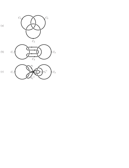
Figure 1: (a) The Borromean rings. The topological significance of this arrangement is that while no pair of loops is linked, the triple of loops is linked. This is the simplest configuration with zero first order (Gaussian) linking and nonzero second order linking. (b) To obtain this figure from (a), pull $C_{1}$ and $C_{2}$ apart for flexible $C_{3}$. (c) To obtain this figure from (b), pinch $C_{3}$ at the point $x_{0}$ so that it becomes a commutator loop $C_{3}=a_{1}a_{2}a_{1}^{-1}a_{2}^{-1}$.

To see the higher order linking in more detail, we let ring $C_{3}$ be flexible and pull rings $C_{1}$ and $C_{2}$ apart while keeping their shapes fixed. This gives Fig. 1b. Next, we pinch the lines of ring $C_{3}$ in Fig. 1b together at point $x_{0}$ to form Fig. 1c Hatcher . Now we follow the semiclassical path of ring $C_{3}$ to see how it is linked with rings $C_{1}$ and $C_{2}$. From Fig. 1c we see that we get four components: $a_{1}$, followed by $a_{2}$, followed by $a_{1}^{-1}$, and then by $a_{2}^{-1}$. Here $a_{1}$ links through $C_{1}$ and $a_{2}$ links through $C_{2}$ in the positive sense respectively, while $a_{1}^{-1}$ and $a_{2}^{-1}$ link through $C_{1}$ and $C_{2}$ in the negative sense pi1 . So the entire path $C_{3}$ runs through $C_{1}$ once in the positive and once in the negative sense for a total Gaussian linking of zero with $C_{1}$. Likewise, there is no Gaussian linking with $C_{2}$. But the total path $C_{3}$ is not trivial. This is because the paths $a_{1}$ and $a_{2}$ do not commute. In fact, $C_{3}$ is just the commutator, which we can write in multiplicative form as $C_{3}=a_{1}a_{2}a_{1}^{-1}a_{2}^{-1}$. It is this commutator that leads to a new phase. To see this, we must introduce a physical system that displays the properties we have been describing. We need the topology of Fig. 1, but in such an arrangement that loop $C_{3}$ corresponds to the path of a particle and loops $C_{1}$ and $C_{2}$ to solenoids. This should not be difficult to arrange experimentally, and a sketch is provided in Fig. 2.

In the Aharonov-Bohm case, the wave function along a path $\varGamma$ can be written as $\psi({\bm{A}})=\psi(0)\exp{({i\int_{\varGamma}{\bm{A}\cdot}d{\bm{x}}})}$, where we are using natural units $\hbar=c=1$ with unit charge to simplify the analysis, but will restore physical units when we reach our results. The interference between wave amplitudes from the two semiclassical paths $C^{\prime}$ and $C^{\prime\prime}$ around a closed path $C=C^{\prime}{C^{\prime\prime}}^{-1}$ is

$$\psi({\bm{A}})=\psi^{\prime}({\bm{A}})+\psi^{\prime\prime}({\bm{A}})=e^{i\beta}\left[\psi^{\prime}(0)+e^{i\phi}\psi^{\prime\prime}(0)\right],$$ (1)

where $\beta$ is an overall irrelevant phase and the important relative phase is

$$\phi=\oint_{C=\partial S}{\bm{A}}\cdot d{\bm{x}}=\int_{S}{\bm{B}}\cdot d{\bm{S}}=\frac{e\varPhi}{\hbar c}.$$ (2)

in SI units, where $\varPhi$ is the magnetic flux enclosed in the solenoid.

Now let us return to the Borromean ring configuration and follow the semiclassical path of a particle around the circuit $C_{3}$ where we now take $C_{1}$ and $C_{2}$ to be a pair of unlinked solenoids. If, and only if, the particle path has no net first order linking with either solenoid $C_{1}$ or $C_{2}$, will we then define a gauge Massey , Berger that describes the higher order linking gauge comment . That gauge is

$${\bm{A}_{12}}=\tfrac{1}{2}(\gamma_{1}{\bm{A}_{2}}-\gamma_{2}{\bm{A}_{1}}),$$ (3)

where subscripts 1 and 2 refer to the solenoids along $C_{1}$ and $C_{2}$, and

$$\gamma_{k}=\delta_{k}+\int_{\varGamma}{\bm{A}_{k}\cdot}d{\bm{x}}.$$ (4)

Here ${\bm{A}_{1}}$ and ${\bm{A}_{2}}$ are the vector potentials due to the two solenoids, and $\varGamma$ is the path that will run along $C_{3}$.

We now want to calculate the overall phase difference $K^{-1}\phi_{12}=\int_{C_{3}}{\bm{A}}_{12}\cdot d{\bm{x}}$. (The $K^{-1}$ normalization factor multiplying $\phi_{12}$ will be discussed below.) Table 1 follows the path step by step through the experimental setup along path $C_{3}$ using the gauge ${\bm{A}_{12}}$.

Table 1: Phase components along the path $C_{3}$.

path segment $\varGamma$	$\gamma_{1}$	$\gamma_{2}$	$K^{-1}\phi_{12}(\varGamma)$
$1$	$\delta_{1}$	$\delta_{2}$	$0$
$a_{1}$	$\delta_{1}+\varPhi_{1}$	$\delta_{2}$	$-\frac{1}{2}\varPhi_{1}\delta_{2}$
$a_{1}a_{2}$	$\delta_{1}+\varPhi_{1}$	$\delta_{2}+\varPhi_{2}$	$\frac{1}{2}[(\delta_{1}+\varPhi_{1})\varPhi_{2}-\varPhi_{1}\delta_{2}]$
$a_{1}a_{2}a_{1}^{-1}$	$\delta_{1}$	$\delta_{2}+\varPhi_{2}$	$\frac{1}{2}[(\delta_{1}+\varPhi_{1})\varPhi_{2}-\varPhi_{1}\delta_{2}+\varPhi_{1}(\delta_{2}+\varPhi_{2})]$
$C_{3}=a_{1}a_{2}a_{1}^{-1}a_{2}^{-1}$	$\delta_{1}$	$\delta_{2}$	$\varPhi_{1}\varPhi_{2}$

The first column labels the current positions on the path, the next two columns are the cumulative values of $\gamma_{1}$ and $\gamma_{2}$ at these points, and the last column gives the value of $\phi_{12}(\varGamma)$ at these points. In the third row we have used $a_{1}$ to take us from $x_{0}$ around $C_{1}$ and back to $x_{0}$. In the process $\gamma_{1}$ has increased by $\varPhi_{1}$ since $\int_{\varGamma=a_{1}}{\bm{A}_{1}}\cdot d{\bm{x}}=\varPhi_{1}$ while $\gamma_{2}$ stays fixed since $\int_{\varGamma=a_{1}}{\bm{A}_{2}\cdot}d{\bm{x}}=0$. Hence we have

$$K^{-1}\phi_{12}(a_{1})=\tfrac{1}{2}\gamma_{1}\int_{\varGamma=a_{1}}{\bm{A}_{2}\cdot}d{\bm{x}}-\tfrac{1}{2}\gamma_{2}\int_{\varGamma=a_{1}}{\bm{A}_{1}\cdot}d{\bm{x}}=-\tfrac{1}{2}\varPhi_{1}\delta_{2}.$$ (5)

From here it is obvious how to generate the remaining entries in the table.

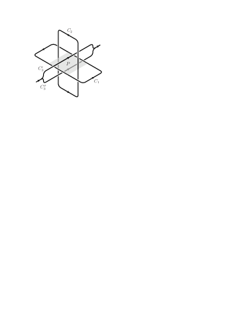
Figure 2: Shown is a schematic of a Borromean ring arrangement to detect the second order phase $\phi_{12}$, where $C_{1}$ and $C_{2}$ are magnetic solenoids (leads not shown) carring flux $\varPhi_{1}$ and $\varPhi_{2}$, and $C_{3}^{\prime}$ and $C_{3}^{\prime\prime}$ correspond to two topologically distinct paths and are parts of the closed path $C_{3}=C^{\prime}_{3}{C^{\prime\prime}_{3}}^{-1}$ of a charged particle path starting from the source and ending at the screen. To prevent second order (gaussian) linking of the wave function with the solenoids one would install a rectangular plate $P$ in the plane of $C_{1}$ that covers the area between the two sides of $C_{1}$ and fills the region between the sides of $C_{2}$. For particle wave packets that do not spread much beyond the center of the region containing the plate, only second order linking will be detected at the screen.

Figure 3: Graphic representation of the information in Table I.

An alternative representation of this information is given in Fig. 3. Here the path $C_{3}$ begins at the initial position $(\delta_{1},\delta_{2})$. We first use $a_{1}$ to travel to $(\delta_{1}+\varPhi_{1},\delta_{2})$, picking up an area $\delta_{2}\varPhi_{1}$, which corresponds to a contribution of $-\frac{1}{2}\delta_{2}\varPhi_{1}$ to $K^{-1}\phi_{12}$ (see Eq. (3)). Next, $a_{2}$ takes us to $(\delta_{1}+\varPhi_{1},\delta_{2}+\varPhi_{2})$ and it generates a contribution $\frac{1}{2}(\delta_{1}+\varPhi_{1})\varPhi_{2}$. Next, $a_{1}^{-1}$ takes us to $(\delta_{1},\delta_{2}+\varPhi_{2})$ and contributes $\frac{1}{2}\varPhi_{1}(\delta_{2}+\varPhi_{2})$. Finally, $a_{2}^{-1}$ returns us to $(\delta_{1},\delta_{2})$ and contributes $-\frac{1}{2}\delta_{1}\varPhi_{2}$, for a total phase of $K^{-1}\phi_{12}=\varPhi_{1}\varPhi_{2}$ for traversing the full loop $C_{3}$. The last row of Table 1 (or the full loop in Fig. 1c) gives the final result for the full path when $\varGamma=C_{3}$. We find

$$\phi_{12}(C_{3})=K\frac{e^{2}}{\hbar^{2}c^{2}}\varPhi_{1}\varPhi_{2}$$ (6)

once physical units have been restored. Figure 2 provides a schematic of the Borromean ring experimental setup with two solenoidal rings and split charged particle path.

Equation (6) is our main result and may be surprising in several respects. First and foremost, $\phi_{12}(C_{3})$ does not vanish, even though the wave function has no first order linking with either solenoid. Second, the overall phase is proportional to the product of the fluxes from the two solenoids. Third, the result is not difficult to generalize to more complicated paths with multiple second order linking as we will show below, and to higher order of linking as we will show elsewhere BK .

Before proceeding let us finally discuss normalization factor in the phase. Recall Dirac’s magnetic monopole requires a string (return flux tube). The string can be made unobservable if it carries an integer number of flux quanta. Likewise the Aharonov-Bohm phase is unobservable if the phase shift is a multiple of $2\pi$, and the magnetic flux enclosed by the particle paths is an integer multiple of the flux quantum. In Fig. 2 we make a similar requirement. If both $C_{1}$ and $C_{2}$ carry quantized flux, i.e., if both $\frac{e\varPhi_{1}}{\hbar c}$ and $\frac{e\varPhi_{2}}{\hbar c}$ are integer multiples of $2\pi$, then we expect the second order linking to be unobservable 2pi . This is the case if we include the $K=\frac{1}{2\pi}$ normalization factor 2pi2 in Eq. (6).

Before concluding let us explore the case of multiple second order linking. Again, consider two unlinked closed rings $C_{1}$ and $C_{2}$ and a third path $C$ that will wrap around them. $C$ starts at point $x_{0}$ and then wraps via subpaths $a_{1}$ and $a_{2}$ some number of times. We define a lattice space of paths where $a_{1}$, $a_{2}$, $a_{1}^{-1}$ and $a_{2}^{-1}$ are right, up, left, and down steps by one lattice spacing, respectively. For example, consider the first frame in Fig. 4, where $\tilde{C}=a_{1}^{3}a_{2}^{2}a_{1}^{-2}$. The accumulated first order linking $\tilde{\phi}_{k}$ is the total number of times $C$ wraps around $C_{k}$ ($k=1,2$), i.e., the projected distance on the $k$-axis from the starting point. Here $\tilde{\phi}_{1}=1$ and $\tilde{\phi}_{2}=2$. But notice the path is not closed, and so ${\bm{A}_{12}}$ cannot be defined, and there can be no second order linking. Next note that any closed path has no net first order linking, i.e., the net numbers of horizontal and vertical moves are both zero, but this is just when we can define ${\bm{A}_{12}}$. Now consider the closed path in the second frame of Fig. 4, where $C=a_{1}^{3}a_{2}^{2}a_{1}^{-2}a_{2}a_{1}^{-1}a_{2}^{-3}$. This path can be written as a product of commutators, $C=C^{(1)}C^{(2)}C^{(3)}$, where the commutators are themselves closed paths (see the bottom row of Fig. 4). The total accumulated phase for $C$ is the sum of those for $C^{(1)}$, $C^{(2)}$, $C^{(3)}$; in this case, $\phi_{12}=6-2+3=7$, and this corresponds to the total number of cells of the lattice enclosed by path $C$. (Recall that the simple Borromean ring commutator is $a_{1}a_{2}a_{1}^{-1}a_{2}^{-1}$, which encloses one lattice cell.) The result for enclosed flux by an arbitrary closed path $C$ is

$$\phi_{12}=nK\frac{e^{2}}{\hbar^{2}c^{2}}\varPhi_{1}\varPhi_{2},$$ (7)

where $n$ is the number of cells enclosed by the path.

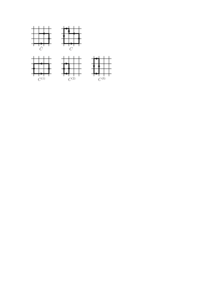
Figure 4: Paths in lattice space generated by $a_{1}$ and $a_{2}$. Open paths have first order linking, closed paths do not.

In summary, first order (Gaussian) linking leads to interference with phase proportional to enclosed flux in the case of the Aharonov-Bohm effect. Higher order linking also leads to interference, but with phases proportional to products of fluxes from different solenoids. Even though path components $a_{1}$ and $a_{2}$ in the above example do not commute, the phase is still abelian as required path-integral . Our analysis needs nothing more than quantum mechanics and a judicious choice of gauge, and our conclusions are easily testable with tabletop experiments using known techniques.

- (1) Y. Aharonov and D. Bohm, Phys. Rev. 115, 485 (1959).
- (2) D. Rolfsen, Knots and Links, Publish or Perish, Wilmington, DE, 1976.
- (3) A. Hatcher, Algebraic topology, Cambridge University Press, Cambridge, 2002.
- (4) and are generators of the fundamental group of the space . If and are unlinked, then , where indicates the free product free-groups . Paths with vanishing first order linking correspond to elements of the commutator subgroup of .
- (5) T. T. Wu and C. N. Yang, Phys. Rev. D 12, 3845 (1975).
- (6) W. S. Massey, Symp. Int. Topologia Algebraica, Mexico, 145 (1959); W. S. Massey, Proc. Conf. on Algebraic Topology, Chicago, University of Illinois at Chicago, p. 174 (1968); D. Kraines, Trans. Amer. Math. Soc. 124, 431 (1966); E. J. O’Neill Trans. Amer. Math. Soc. 248, 37 (1979); R. A. Fenn, Techniques of Geometric Topology, Cambridge University Press, Cambridge, 1983; M. I. Monastyrsky and V. S. Retakh, Commun. Math. Phys. 103, 445 (1986).
- (7) M. A. Berger, J. Phys. A, 23, 2787 (1990).
- (8) is a closed path for the (first order) choice of gauge used in the Aharonov-Bohm case, but it is only part of the path . At second order, a closed path is a commutator of the generators of closed paths at first order. When the phase depends on the choice of the point and we do not have a closed path, we are not measuring interference since we have not recombined the two halves of the wave function. So one can argue that if we are looking for interference, then we should look for a gauge where we have closed paths, and , , and are not closed for . Since for the AB gauge choice , , and deliver interference, while in they give results dependent on the location of the point , we see may be an allowed gauge choice, but it is not a good choice for these paths. It only becomes a good choice when we are looking at the full commutator path.
- (9) R. V. Buniy and T. W. Kephart, in preparation.
- (10) W. Magnus, A. Karrass, D. Solitar, Combinatorial Group Theory: Presentations of Groups in Terms of Generators and Relations, Interscience, New York, 1966.
- (11) Further discussion of the normalization of generalized phases is in order. For the magnetic field in tube choose a gauge , such that vanishes everywhere except in the disk bounded by , and such that picks up a contribution when punches through the disk. Likewise choose to be nonzero only in the disk bounded by . Then along the intersection line there is a virtual flux tube carrying a total generalized flux of generalized magnetic field directed along the intersection line. In Fig. 2 this corresponds to having a virtual flux tube running along the the long symmetry axis of the curve . Having the path linking with generates the phase . Now imposing the Dirac string condition separately on and i.e., is unobservable if is an integer multiple of , likewise for , and simultaneously imposing the requirement (à la Dirac) that the phase be unobservable and the enclosed generalized flux a multiple of , when the “subfluxes” and are unobservable, fixes the normalization and gives . However, this generalized Dirac condition and its normalization must ultimately be checked by experiment.
- (12) Similarly, we expect higher order cases where the phases are proportional to the product of fluxes to have normalization factors as will be discussed in BK .
- (13) L. S. Schulman, J. Math. Phys. 12, 304 (1971); M. G. G. Laidlaw and C. M. DeWitt, Phys. Rev. D 3, 1375 (1971); L. S. Schulman, Techniques and Applications of Path Integration, Wiley-Interscience, New York, 1981.