de Sitter String Vacua from Kähler Uplifting

Abstract:

We present a new way to construct de Sitter vacua in type IIB flux compactifications, in which the interplay of the leading perturbative and non-perturbative effects stabilize all moduli in dS vacua at parametrically large volume. Here, the closed string fluxes fix the dilaton and the complex structure moduli while the universal leading perturbative quantum correction to the Kähler potential together with non-perturbative effects stabilize the volume Kähler modulus in a $dS_{4}$-vacuum. Since the quantum correction is known exactly and can be kept parametrically small, this construction leads to calculable and explicitly realized de Sitter vacua of string theory with spontaneously broken supersymmetry.

1 Introduction

Much of the recent progress in string theory is connected to the discovery of an enormous number [1, 2, 3, 4] of stable and meta-stable 4d vacua in its low-energy effective supergravities. The advent of this ’landscape’ [3] of isolated, moduli stabilizing minima marks considerable progress in the formidable task of constructing realistic 4d string vacua. In particular, one of the most pressing issues has been how to stabilize the geometrical moduli of a compactification, and at the same time address the tiny, positive cosmological constant that is inferred from the present-day accelerated expansion of the universe [5]. Recently, the use of closed string background fluxes in string compactifications has been studied in this context [6, 7, 8, 9, 10, 11, 12, 13, 14, 15, 16, 17, 18, 19, 20, 21, 22, 23, 24, 25]. Such flux compactifications can stabilize the dilaton and the complex structure moduli in type IIB string theory. Non-perturbative effects such as the presence of $D$p-branes [26] and gaugino condensation were then used by Kachru et al (henceforth KKLT) [2] to stabilize the remaining Kähler moduli in such type IIB flux compactifications (for related earlier work in heterotic M-theory see [27]). Simultaneously these vacua allow for SUSY breaking and thus the appearance of metastable $dS_{4}$-minima with a small positive cosmological constant fine-tuned in discrete steps. KKLT [2] used the SUSY breaking effects of an $\overline{D3}$-brane to achieve this. Alternatively the effect of D-terms on $D7$-branes has been considered in this context [28].

Bearing in mind the importance of constructing 4d de Sitter string vacua in a reliable way, one should note the problems of using $\overline{D3}$-branes as uplifts for given volume-stabilizing AdS minima. The SUSY breaking introduced by an $\overline{D3}$-brane is explicit and the uplifting term it generates in the scalar potential cannot be cast into the form of a 4d ${\cal N}=1$ supergravity analysis. Thus, the control that we have on possible corrections in supergravity is lost once we use $\overline{D3}$-branes for SUSY breaking. Replacing them by D-terms driven by gauge fluxes on $D7$-branes [28] is one way to alleviate this problem because then the SUSY breaking is only spontaneous (for a detailed study of the D-terms from magnetized $D7$-branes see e.g. [29]). In this case the requirements of both 4d supergravity and the $U(1)$ gauge invariance necessary for the appearance of a D-term place consistency conditions on the implementation of a D-term (noted in [28], and emphasized in [30, 31, 32, 33]). These conditions have not yet been met by any concrete stringy realization of [28], where the proposal was made in the context of KKLT. More recently, progress has been made in finding ways of having a D-term uplift co-existing consistently with non-perturbative Kähler moduli stabilization both in 4d supergravity [33] and in more stringy contexts [32, 34, 35, 36, 37, 38]. Note, that the implementation of a consistent D-term uplift becomes considerably simplified [39] in the case, that the stabilization of the volume proceeds perturbatively through an interplay of the leading $\alpha^{\prime}$- and string loop corrections to the Kähler potential [40, 41] (related work in the context of 5D supergravity appeared in [42]). Since the calculation of the string loop correction (which has to be carried out for each Calabi-Yau anew) is technically challenging [43], it is not clear how far this dS vacua from Kähler stabilization generalizes.

In view of this situation it becomes appealing to look for a possibility of F-terms generating the dS vacuum. Four lines of access have been studied here: Firstly, one may use the SUSY breaking $(0,3)$ ISD $G_{(3)}$-fluxes of type IIB flux compactifications to stabilize the complex structure moduli in (metastable) minima of non-vanishing F-term [44]. Secondly, one may use F-terms coming from the interactions of hidden sector matter fields to uplift AdS minima towards de Sitter [45] (for a related discussion of dS vacua in M-theory see [46]). The third way considers strong gauge dynamics. This can lead to the existence of metastable F-term SUSY breaking minima along the lines of the ISS proposal [47] which may then be used for uplifting purposes [48, 49]. The effective description of these metastable vacua can be done in terms of generalized O’Raifaertaigh models which has been studied in the context of KKLT recently in [50, 51]. These constructions provide examples of a general analysis of 4d ${\cal N}=1$ supergravity with an F-term uplifting sector which is separated from the moduli sector [52]. The fourth path, which will be pursued in this paper consists of using the leading correction to the Kähler potential given by an ${\cal O}(\alpha^{\prime 3})$-correction [53]. The $\alpha^{\prime}$-correction has recently been used to provide a realization of the simplest KKLT $dS$-vacua with, however, either ${\cal O}(1)$ volume [54] or considerably large values of the $\alpha^{\prime}$-correction [55]. A combination of the contributions to the scalar potential from D-branes and the $\alpha^{\prime}$-correction can also be used to stabilize the volume modulus in a dS minimum [56] (related discussions of the effect of Kähler corrections on the stabilization of light moduli appear in [57]).

The present work, which extends the results of Balasubramanian & Berglund [54], will show that in type IIB flux compactifications the interplay of the leading non-perturbative contributions to the superpotential and the leading $\alpha^{\prime}$-correction to the Kähler potential can lead to volume stabilization in a dS minimum at parametrically large volume while keeping the value of the $\alpha^{\prime}$-correction parametrically small. To get the volume at large values it is necessary to have the rank of the condensing gauge group living on a stack of D7-branes wrapping the 4-cycle dual to the volume modulus at larger values of ${\cal O}(30\ldots 100)$. We will then show that this dS vacuum persists after including the flux stabilization of the dilaton and the complex structure moduli. Thus, the setup will be shown to lead to a full stabilization of all geometric moduli in a parametrically controllable, metastable dS minimum which breaks supersymmetry spontaneously through non-vanishing F-terms. Since the vacuum energy of this dS vacuum is controlled by the magnitude of the flux superpotential, the cosmological constant can be fine-tuned by virtue of the large number of 3-cycles of generic type IIB flux compactifications. Finally, we will show that the quintic $C\mathbb{P}^{4}_{1,1,1,1,1}$ provides a reasonably explicit example realizing this construction of dS vacua from Kähler uplifting. This illustrates the fact, that due to the universal nature of the leading $\alpha^{\prime}$-correction (which contributes on every Calabi-Yau with non-zero Euler number $\chi$) these Kähler uplifted dS vacua should exist on all Calabi-Yau 3-folds with $\chi<0$ and arithmetic genus $\chi(D)=1$ [58]. Here $D$ denotes the divisor of the corresponding 4-fold in F-theory which projects back to the 4-cycle dual to the volume modulus. Of course, an appropriate choice of fluxes is necessary to get the dilaton stabilized at weak coupling and to tune the arising dS minimum to nearly zero vacuum energy.

The paper is organized as follows. Section 2 reviews the leading quantum correction to the Kähler potential of type IIB flux compactifications as well as the general argument that the combined effect of the leading perturbative correction to the Kähler potential and the leading non-perturbative contribution to the superpotential can produce volume stabilization in a metastable dS minimum. These results are then used in Section 3 to show that this structure can be extended to shift the stabilized volume to (in principle) arbitrarily large values. We proceed then in Section 4 to demonstrate that upon the inclusion of flux stabilization of the dilaton as well as of the complex structure moduli we arrive at a full stabilization of all geometric moduli in a true dS minimum which succeeds in keeping the volume parametrically large and the Kähler correction small. This is done using an explicit example given by the quintic hypersurface $C\mathbb{P}^{4}_{1,1,1,1,1}$ providing evidence that these Kähler uplifted metastable $dS$-vacua can be explicitly realized in type IIB string theory, and are thus expected to exist for all Calabi-Yau 3-folds with $h^{2,1}>h^{1,1}=1$, at least. We extend these results to other examples of Calabi-Yau 3-folds with $h^{1,1}=1$. Finally, we discuss and summarize our results in the Conclusion.

2 The leading $\alpha^{\prime}$-correction in KKLT

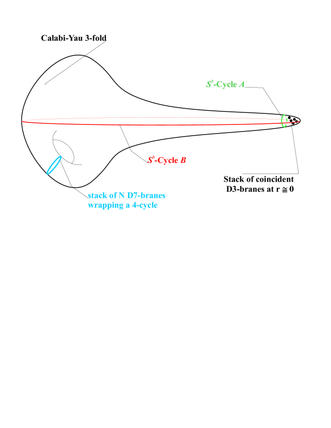
Our discussion will take place in the framework of type IIB string theory compactified to 4d on orientifolded Calabi-Yau threefolds in the presence of RR and NS-NS closed-string background fluxes along the lines of [6]. Thus, it will prove to be useful to recall some of the main results here. Non-zero background flux quantized on the 3-cycles of the Calabi-Yau requires the presence D3-branes or 4-cycle wrapping D7-brane to source the flux and induces a non-trivial warpfactor in the internal dimensions. This leads to a geometry - visualized in Fig. 1 - where the warped manifold is conformally Calabi-Yau. Under certain conditions it develops a region warped into an approximate AdS throat region which ends in the UV on the bulk of the Calabi-Yau and is capped off smoothly in the IR by an appropriate analogue of the Klebanov-Strassler solution.

Figure 1: Flux induced warped Calabi-Yau geometry in type IIB.

A very helpful property of these flux compactifications is the fact that the equations of motion force the 3-form flux $G_{(3)}$ to be ISD and primitive in the $(1,2)$- or $(0,3)$-cohomology classes of the Calabi-Yau. Simultaneously the back-reaction on the geometry is confined to driving the non-trivial warpfactor [6]. This we can see from the equations of motion for the 5-form field strength $\tilde{F}_{(5)}$ and the metric in the combination

$$\tilde{\nabla}^{2}(e^{4A}-\alpha)=e^{2A}\frac{|iG_{(3)}-\ast_{6}\bar{G}_{(3)}|^{2}}{6\;\textrm{Re}\,S}+e^{-6A}\left|\partial(e^{4A}-\alpha)\right|^{2}+2\kappa_{10}^{2}e^{2A}\left[\frac{1}{4}\,(T_{m}^{m}-T_{\mu}^{\mu})^{\textrm{loc}}-\mu_{3}\overline{\rho_{3}^{\textrm{loc}}}\right]$$ (1)

since the vanishing of the LHS requires the D-branes and O-planes as the sources of flux to fulfill a pseudo-BPS condition and $G_{(3)}$ to be ISD. This forces then $G_{(3)}$ to be of $(1,2)$ or $(0,3)$ type and ensures that we stay in a geometry which is conformally the same as the flux-less original Calabi-Yau. The fluxes stabilize the type IIB axio-dilaton and the complex structure moduli $U^{\alpha}$. This is encoded by the fact that the fluxes generate a Gukov-Vafa-Witten type superpotential [12] in the 4d effective supergravity description

$$W_{\rm flux}=\frac{1}{2\pi}\,\int_{\rm CY_{3}}G_{(3)}\wedge\Omega=:W_{0}\;\;.$$ (2)

Then the fact that $G_{(3)}$ being of $(1,2)$ or $(0,3)$ type keeps the back-reaction confined to the warpfactor implies that the flux superpotential can take values larger than ${\cal O}(1)$ while we remain within the same supergravity solution. This will be very helpful in the ensuing discussion.

Stabilization of the remaining Kähler moduli - which at tree-level are no-scale - is then possible along the lines of KKLT [2] by inclusion of the leading non-perturbative effects in the superpotential like instantons from Euclidean $D3$-branes wrapping 4-cycles of the Calabi-Yau or gaugino condensation on 4-cycle wrapping stacked $D7$-branes. Thus, the corresponding 4d ${\cal N}=1$ supergravity given by [2]

$$K = -2\ln{\hat{\cal V}}-\ln(S+\bar{S})-\ln\left(-i\int_{\rm CY_{3}}\bar{\Omega}\wedge\Omega\right)$$

$$W = W_{\rm flux}+\sum_{i}A_{i}e^{-a_{i}T_{i}}$$ (3)

generically manages to stabilize all geometric moduli and the dilaton in a SUSY AdS minimum.

Here $\hat{\cal V}$ denotes the volume of the Calabi-Yau in Einstein frame which is defined as $\hat{\cal V}=\frac{1}{6}\,\kappa_{jkl}\,\hat{t}^{j}\hat{t}^{k}\hat{t}^{l}$ in terms of the $h^{1,1}$ 2-cycle moduli $\hat{t}^{j}$ and the intersection numbers $\kappa_{jkl}$. The 4-cycle Kähler moduli $T_{j}$ are then defined by [53, 56] $T_{j}=\frac{1}{3}\,\partial_{\hat{t}^{j}}\hat{\cal V}+i\int_{D_{j}}C_{(4)}=:T_{j,r}+i\tau_{j}$ where $D_{j}$ denotes the divisor 4-cycle with volume ${\rm Re}\,T_{j}$ and $\hat{\cal V}$ is thus a function of the $T_{i}$ defined implicitly through the inverse of the former relations. For the following discussions we will assume for simplicity the presence of just one Kähler modulus $T$ measuring the overall volume $\hat{\cal V}$ as it is realized, e.g., by the quintic example $C\mathbb{P}^{4}_{1,1,1,1,1}$. Then we have $\hat{\cal V}=\frac{\kappa}{6}\,\hat{t}^{3}=\gamma\,(T+\bar{T})^{3/2}$ where we defined $\gamma=\frac{\sqrt{3}}{2\sqrt{\kappa}}$.

In addition to the leading non-perturbative effects we have now the leading perturbative correction to the Kähler potential of the Kähler moduli arising from the universal ${\cal O}(\alpha^{\prime 3})$ $R^{4}$-correction to the 10d type IIB supergravity action [53, 59]

$$S_{\textrm{IIB}} = -\frac{1}{2\kappa_{10}^{2}}\int d^{10}x\sqrt{-g_{\textrm{s}}}\;e^{-2\phi}\left[R_{\textrm{s}}+4\left(\partial\phi\right)^{2}+\left.\alpha^{\prime}\right.^{3}\frac{\zeta(3)}{3\cdot 2^{11}}\;J_{0}\,+\,\ldots\,\right]\;\;.$$ (4)

Here $J_{0}$ denotes the higher-derivative interaction

$$J_{0}=\left(t^{M_{1}N_{1}\cdots M_{4}N_{4}}t_{M_{1}^{\prime}N_{1}^{\prime}\cdots M_{4}^{\prime}N_{4}^{\prime}}+\frac{1}{8}\;\epsilon^{ABM_{1}N_{1}\cdots M_{4}N_{4}}\epsilon_{ABM_{1}^{\prime}N_{1}^{\prime}\cdots M_{4}^{\prime}N_{4}^{\prime}}\right)\left.R^{M_{1}^{\prime}N_{1}^{\prime}}\right._{M_{1}N_{1}}\cdots\left.R^{M_{4}^{\prime}N_{4}^{\prime}}\right._{M_{4}N_{4}}\;,$$

and the tensor $t$ is defined in [60]. This generates a corrected Kähler potential of the Kähler moduli [53]

$$K = -2\cdot\ln\left({\cal\hat{V}}+\alpha^{\prime 3}\frac{\hat{\xi}}{2}\right)\;,\;\;\;\hat{\xi}=-\frac{\zeta(3)}{4\sqrt{2}(2\pi)^{3}}\;\cdot\chi\cdot(S+\bar{S})^{3/2}=:\xi\cdot(S+\bar{S})^{3/2}\;\;.$$ (5)

Here ${\cal\hat{V}}=\gamma\,(T+\bar{T})^{3/2}$ denotes the Calabi-Yau volume in Einstein frame, $\chi$ is the Euler number of the Calabi-Yau and from now on we set $\alpha^{\prime}=1$.

The inclusion of this correction into the class of models defined by eq. (3) has been shown to lead either to non-SUSY AdS minima for the Kähler moduli at exponentially large volumes [61] or to non-SUSY Minkowski and dS minima at small volume $\hat{\cal V}\sim 2$ [54] without the need of either $\overline{D3}$-branes or D-terms. We shall now summarize the construction of the latter by Balasubramanian & Berglund [54] since their general argument for the existence of dS vacua in the $\alpha^{\prime}$-corrected theory forms the starting point for the further discussion.

Prior to the inclusion of the above leading $\alpha^{\prime}$-correction we have a SUSY AdS minimum for all moduli $U^{\alpha}$, $S$ and $T$ given by $D_{T}W=0$ in the supergravity of eq. (3). Now, in the KKLT regime of $|W_{0}|\ll 1$, $W_{0}<0$ turning on the correction by giving $\hat{\xi}$ some value still gives a solution to the corrected $D_{T}W=0$ as long as the $\alpha^{\prime}$-expansion parameter $\hat{\xi}/(2\,\hat{{\cal V}})$ is small in the minimum. Now increase $|W_{0}|$. Increasing $|W_{0}|$ will shift the solution to the full $\alpha^{\prime}$-corrected SUSY condition $D_{T}W=0$ to ever smaller values of $T$. Hence, there is a value $|W_{0}|=W_{\rm crit}$ where the solution to $D_{T}W=0$ will give $\hat{\cal V}=\hat{\xi}$. At $\hat{\cal V}=\hat{\xi}$, the induced scalar potential [53, 54]

$$V_{F}(T)=e^{K}\,\left(K^{i\bar{j}}D_{T_{i}}W\overline{D_{T_{j}}W}-3|W|^{2}\right)$$ (6)

has a singularity. Thus, for $|W_{0}|=W_{\rm crit}-\epsilon$ we have a SUSY AdS minimum at $\hat{\cal V}>\hat{\xi}$ in the geometric region of moduli space while for $|W_{0}|=W_{\rm crit}+\epsilon$ this SUSY stationary point has passed through $\hat{\cal V}=\hat{\xi}$ towards $\hat{\cal V}<\hat{\xi}$.

However, we have that $\lim_{\hat{\cal V}\to\hat{\xi}^{+}0}V_{F}=+\infty$ and due to the dominance of the perturbative $\alpha^{\prime}$-correction over the non-perturbative superpotential terms at large volume we have $V_{F}$ approaching zero from above for $\hat{\cal V}\to\infty$. Furthermore, the scalar potential eq. (6) is a continuous function of $W_{0}$ for all $\hat{\cal V}\neq\hat{\xi}$. In addition, for very large $|W_{0}|$ the non-perturbative contribution to $W$ becomes negligible implying that then

$$V_{F}(T)=e^{K}\cdot 3\hat{\xi}\cdot\frac{\hat{\xi}^{2}+7\hat{\xi}\hat{\cal V}+\hat{\cal V}^{2}}{(\hat{\cal V}-\hat{\xi})(\hat{\xi}+2\hat{\cal V})^{2}}\,|W_{0}|^{2}$$ (7)

which is positive definite and decreases monotonically from $\infty$ to $0$ for $\hat{\cal V}>\hat{\xi}$. Together, this implies that after increasing $|W_{0}|$ from $|W_{0}|=W_{\rm crit}-\epsilon$ to $|W_{0}|=W_{\rm crit}+\epsilon$ there will be a non-supersymmetric AdS minimum for $T$ at $\hat{\cal V}>\hat{\xi}$. Upon increasing $|W_{0}|$ further this non-SUSY AdS minimum will eventually become a Minkowski and subsequently a dS minimum before disappearing altogether. This general argument shows that there is a regime where the combination of the leading perturbative effects in $K$ and the leading non-perturbative effects in $W$ lead to dS vacua without the need for a D-term or an uplifting $\overline{D3}$-brane.

A toy example was given in [54] where the choice of $A=1$, $a=2\pi/10$, $W_{0}=-1.7$ and $\hat{\xi}\approx 0.4$ (as it is the case, e.g., for the quintic with $\chi=-200$ if we assume $S$ stabilized at ${\rm Re}\,S=1$) led to the existence of a dS minimum for ${\rm Re}\,T$ at ${\rm Re}\,T\approx 5$ corresponding to $\hat{\cal V}\approx 2$. The stabilization of $S$ and the complex structure moduli was assumed there.

In the main part of this paper we will now show that, firstly, certain scaling properties of the scalar potential allow us to stabilize the physical volume $\hat{\cal V}$, measured in Einstein frame, at values of ${\cal O}(10^{2}\ldots 10^{3})$ by fixing the dilaton at weak coupling $g_{S}=({\rm Re}\,S)^{-1}\sim 0.1$. Secondly, the stabilization of the dilaton $S$ and the complex structure moduli $U^{\alpha}$ (at least for the case of a single $U$) can be done explicitly in the above context. Simultaneously, all axionic directions are shown to get lifted as well.

3 Parametrically controllable Kähler uplifting and dS vacua

The starting point of the ensuing discussion is the fact that the $\alpha^{\prime}$-corrected Kähler potential eq. (5) leads to a mixing of the volume and the dilaton in the resulting scalar potential of the theory. Therefore, to begin with we shall have to write down the full F-term scalar potential for the $S$-$T$-moduli sector of the model defined by

$$K = -2\cdot\ln\left({\cal\hat{V}}+\frac{\hat{\xi}}{2}\right)\;\;,\;\hat{\cal V}=\gamma\,(T+\bar{T})^{3/2}$$

$$W = W_{0}+Ae^{-aT}\;\;.$$ (8)

Here $a=2\pi/N$ denotes the beta function of the $SU(N)$ gauge theory living on a stack of $N$ $D7$-branes which undergoes gaugino condensation. We will need the inverse of the Kähler metric $K_{a\bar{b}}$ with $a,b=S,T$ which can be found, e.g., in [56, 61] and is given by

$$K^{a\bar{b}}=\left(\begin{array}[]{ll}\gamma^{-4/3}\frac{\sqrt[3]{\hat{\cal V}}(4\hat{\cal V}^{2}+\hat{\xi}\hat{\cal V}+4\hat{\xi}^{2})}{12(\hat{\cal V}-\hat{\xi})}&-\frac{3(\gamma^{-1}\,\hat{\cal V})^{2/3}\hat{\xi}\text{Re}(S)}{2(\hat{\cal V}-\hat{\xi})}\\ -\frac{3(\gamma^{-1}\,\hat{\cal V})^{2/3}\hat{\xi}\text{Re}(S)}{2(\hat{\cal V}-\hat{\xi})}&\frac{(4\hat{\cal V}-\hat{\xi})\text{Re}(S)^{2}}{\hat{\cal V}-\hat{\xi}}\end{array}\right)\;\;.$$ (9)

The scalar potential then reads

$$V_{F}(S,T) = e^{K}\,\left(K^{a\bar{b}}D_{a}W\overline{D_{b}W}-3|W|^{2}\right)$$ (10)

$$= e^{K}\,\left\{K^{T\bar{T}}[W_{T}\overline{W_{T}}+(W_{T}\cdot\overline{WK_{T}}+c.c.)]\right.$$

$$\;\left.+[K^{T\bar{S}}D_{T}W\overline{D_{S}W}+c.c]+K^{S\bar{S}}|D_{S}W|^{2}\right.$$

$$\left.+3\hat{\xi}\,\frac{\hat{\xi}^{2}+7\hat{\xi}\hat{\cal V}+\hat{\cal V}^{2}}{(\hat{\cal V}-\hat{\xi})(\hat{\xi}+2\hat{\cal V})^{2}}\,|W|^{2}\right\}$$

where in $K_{a}$ and $D_{a}W$ the use of the full corrected Kähler potential is implied. We will now first assume that the dilaton is stabilized by the fluxes in a supersymmetric minimum (this will be justified later on, where we will see that the full solution for $S$ and $T$, in fact, stabilizes $S$ close to the supersymmetric point and we will get $F_{S}\ll F_{T}$ but $m_{S}\gg m_{T}$). Then the scalar potential for $T$ becomes [54]

$$V(T_{r})=e^{K}\,\left\{K^{T\bar{T}}[a^{2}A^{2}e^{-2aT_{r}}+(-aAe^{-aT_{r}}\overline{WK_{T}}+c.c)]+3\hat{\xi}\,\frac{\hat{\xi}^{2}+7\hat{\xi}\hat{\cal V}+\hat{\cal V}^{2}}{(\hat{\cal V}-\hat{\xi})(\hat{\xi}+2\hat{\cal V})^{2}}\,|W|^{2}\right\}\;\;.$$ (11)

Here we used that the $T$-axion is stabilized at $\tau=0$ the same way as in the original KKLT construction since the perturbative correction to $K$ does not depend on $\tau$.

Plugging in here the values $A=1$, $a=2\pi/10$, $W_{0}=-1.7$, and $\hat{\xi}\approx 0.4$ would then reproduce the dS minimum at $\hat{\cal V}\approx 2$ of [54] if we assume ${\rm Re}\,S=1$.

Now, let us note that eq. (11) possesses a scaling property of the following kind: under a rescaling

$$N\to\lambda N\;,\;a=\frac{2\pi}{N}\to\lambda^{-1}a\;,\;T_{r}\to\lambda T_{r}\;,\;\hat{\xi}\to\lambda^{3/2}\hat{\xi}$$ (12)

the scalar potential scales as

$$V_{F}\to\lambda^{-3}V_{F}$$

while its shape remains unchanged up to the fact that the transformation eq (12) stretches it along the $X$-axis.

This scaling behavior allows us to conclude that by choosing a larger gauge group for the gaugino condensate in $W$ and rescaling $T_{r}$ and $\hat{\xi}$ appropriately we can get dS minima for $T$ at parametrically large volumes $\hat{\cal V}={\cal O}(100\ldots 1000)$. To give an example, let us take $W_{0}\approx-1.7$, as before, but for the other parameters  $a=2\pi/100$ and $\hat{\xi}\approx 79.8$ which corresponds to a scaling with $\lambda=10$. In addition, let again $\kappa=5$ as realized later on for $C\mathbb{P}^{4}_{1,1,1,1,1}$.

This choice of numbers then stabilizes $T$ in a dS minimum at parametrically large (compared to the string scale given by $\sqrt{\alpha^{\prime}}$) volume. For the parameters chosen we get ${\rm Re}\,T\approx 49$ which corresponds to $\hat{\cal V}\approx 376$.

Figure 2: Solid black: The F-term scalar potential $V_{F}(T)$ leading to a dS minimum at $T\approx 43$ corresponding to a parametrically large volume $\hat{\cal V}\approx 309$ through the inclusion of the leading perturbative and non-perturbative effects. The choice or parameters here reads $\kappa=5$ (as realized on the quintic), $W_{0}\approx-32.35$, $a=2\pi/100$ and $\hat{\xi}\approx 7.98$. Note the smallness of the $\alpha^{\prime}$-expansion parameter $\hat{\xi}/(2\hat{\cal V})|_{\rm min}\approx 0.01$ in the minimum.

Note that the expansion parameter of the $\alpha^{\prime}$-corrected Kähler potential, $\hat{\xi}/(2\hat{\cal V})$, is invariant under the rescaling eq. (12). It has a value in the above dS minimum of $\hat{\xi}/(2\hat{\cal V})|_{\rm min}\approx 0.1$ which is already small enough to trust the reliability of the $\alpha^{\prime}$-expansion since we neglected higher-order corrections in $\alpha^{\prime}$ to $K$.

However, the reliability of the expansion can be thoroughly improved by noting that the scalar potential eq. (11) allows us trade the size of $\hat{\xi}/(2\hat{\cal V})|_{\rm min}$ for the size of $W_{0}$. Here it is now crucial that, as explained above, having a large $W_{0}$ poses no problematic back-reaction in the type IIB flux compactifications of [6] as there fluxes must be ISD and of $(1,2)$- and $(0,3)$-type which confines the back-reaction to the warp factor.

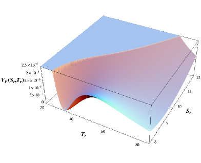
As a demonstration for this we use the explicit example of a parameter choice $\kappa=5$ (as realized on the quintic), $W_{0}\approx-32.35$, $a=2\pi/100$ and $\hat{\xi}\approx 7.98$. This realizes a dS minimum again at $T\approx 43$ but with an expansion parameter $\hat{\xi}/(2\hat{\cal V})|_{\rm min}\approx 0.01$ so small that neglecting the higher-orders in $\alpha^{\prime}$ should now be fully justified. In addition, the non-perturbative contribution to $W$ has a value $\langle A\,\exp(-aT)\rangle\sim 0.05$ which is small enough to trust the validity of the non-perturbative superpotential as well. This result is shown in Fig. 2.

4 The full case - inclusion of $S$ and $U$

The scaling property eq. (12) used in the examples of the previous section clearly neglects the structure of the parameter $\hat{\xi}$ controlling the size of the $\alpha^{\prime}$-correction. $\hat{\xi}$ is not just a parameter but it depends on both $\chi$, the Euler number of the Calabi-Yau, and the value of the dilaton since we have $\hat{\xi}\sim-\chi\,(S+\bar{S})^{3/2}$. Thus, if we speak of rescaling $\hat{\xi}$ this means stabilizing the dilaton at an appropriate value of ${\rm Re}\,S$ since we cannot rescale continuously the discrete, topological quantity $\chi$.

4.1 Stabilizing $S$ and $T$ on the quintic $C\mathbb{P}^{4}_{1,1,1,1,1}$ explicitly

Hence, in order to give a realistic example we shall have to include the stabilization of the dilaton by the fluxes explicitly. The Kähler potential now reads

$$K=-2\cdot\ln\left({\cal\hat{V}}+\frac{\xi}{2}\,(S+\bar{S})^{3/2}\right)-\ln(S+\bar{S})\;\;.$$ (13)

The fluxes induce the GVW superpotential eq. (2) which stabilizes $S$ and the complex structure moduli $U^{\alpha}$.. Its only dependence on $S$ originates in $G_{(3)}=F_{(3)}-S\cdot H_{(3)}$ since the integrals $\int_{\rm CY_{3}}F_{(3)}\wedge\Omega$ and $\int_{\rm CY_{3}}H_{(3)}\wedge\Omega$ in $W_{0}$ are determined entirely by the periods of the Calabi-Yau and thus depend only on the $U^{\alpha}$. After integrating out the $U^{\alpha}$ we can therefore write the superpotential $W_{0}$ with respect to $S$ without loss of generality as

$$W_{0}=C_{1}-C_{2}\cdot S$$ (14)

where we have defined the ($U^{\alpha}$-dependent) constants $C_{1}=\frac{1}{2\pi}\,\int_{\rm CY_{3}}F_{(3)}\wedge\Omega$ and $C_{2}=\frac{1}{2\pi}\,\int_{\rm CY_{3}}H_{(3)}\wedge\Omega$. Integrating out the complex structure moduli is justified at this stage as the next subsection demonstrates that they get masses which are parametrically larger than $S$ and $T$.

In absence of the $\alpha^{\prime}$-correction the supersymmetric stationary point for $S$ is given from $D_{S}W=0$ as

$$S_{0}=-\frac{C_{1}+\langle A\,e^{-aT}\rangle}{C_{2}}\;\;.$$ (15)

Since typically it is $\langle A\,e^{-aT}\rangle\sim 0.1$, $S_{0}$ is determined completely by the flux constants if $|C_{1}|,|C_{2}|>1$.

Turning on the $\alpha^{\prime}$-correction we expect that the true value of the minimum for the dilaton is close by the unperturbed SUSY point, $S_{\rm min}\approx S_{0}$, if we choose $|C_{1}|,|C_{2}|>1$ such that $S_{0}\gg 1$.

As a test this expectation we will now display the complete $S$-$T$-system for the 4 real fields (2 moduli, 2 axions) contained in $T=T_{r}+i\tau$ and $S=S_{r}+i\sigma$. The scalar potential for $S$ and $T$ is then given by eq. (10) as

$$V_{F}(S,T) = e^{K}\,\left\{K^{T\bar{T}}[W_{T}\overline{W_{T}}+(W_{T}\cdot\overline{WK_{T}}+c.c.)]\right.$$ (16)

$$\;\left.+[K^{T\bar{S}}D_{T}W\overline{D_{S}W}+c.c]+K^{S\bar{S}}|D_{S}W|^{2}\right.$$

$$\left.+3\hat{\xi}\,\frac{\hat{\xi}^{2}+7\hat{\xi}\hat{\cal V}+\hat{\cal V}^{2}}{(\hat{\cal V}-\hat{\xi})(\hat{\xi}+2\hat{\cal V})^{2}}\,|W|^{2}\right\}$$

For the sake of explicitness we will take parameters which derive from the Calabi-Yau given by the quintic $C\mathbb{P}^{4}_{1,1,1,1,1}$ which is given by the vanishing locus of the polynomial

$$z_{1}^{5}+z_{2}^{5}+z_{3}^{5}+z_{4}^{5}+z_{5}^{5}=0\;\;.$$ (17)

This threefold has $h^{1,1}=1$, $\kappa=5$ and $\chi=-200$. An orientifold with $O3$- and $O7$-planes can be formed from this manifold by using, e.g., the projection [62]

$${\cal O}=(-1)^{F_{L}}\Omega_{P}\,\sigma^{\ast}\;\;{\rm with}\;\;\sigma:\;\{z_{1},z_{2},z_{3},z_{4},z_{5}\}\to\{z_{2},z_{1},z_{3},z_{4},z_{5}\}$$ (18)

where the holomorphic involution $\sigma$ acts on the holomorphic 3-form $\Omega$ as $\sigma^{\ast}\Omega=-\Omega$. For this Calabi-Yau we get $\xi=0.17133$ and we will further use the choice of flux parameters $C_{1}=-13.743$ and $C_{2}=1.4$ as well as $A=1$ and $a=2\pi/100$ for the non-perturbative sector. For these values we expect then the minimum for $S$ to be close to $S_{0}\approx 9.8$.

Figure 3: The F-term scalar potential $V_{F}(S,T)$ leading to a dS minimum at $T\approx 33.3$ and $S\approx 7.9$ corresponding to a parametrically large volume $\hat{\cal V}\approx 211$ and weak string coupling $g_{S}\approx 0.1$ through the inclusion of the leading perturbative and non-perturbative effects. The choice of the Calabi-Yau, the quintic, gives the parameters $\kappa=5$, $\chi=-200$ and thus $\xi=0.17133$. Further it is chosen $a=2\pi/100$, $A=1$ and $C_{1}=-13.743$ and $C_{2}=1.4$. Note the smallness of the $\alpha^{\prime}$-expansion parameter $\hat{\xi}/(2\hat{\cal V})|_{\rm min}\approx 0.03$ in the minimum.

An analysis of the model yields a dS minimum for all 4 real scalars at

$$T_{r}\approx 33.3\;,\;S_{r}\approx 7.9\;,\;\tau=\sigma=0$$ (19)

and thus at weak string coupling $g_{S}\approx 0.1$ and large volume $\hat{\cal V}\approx 211$. The fact, that this stationary point of the scalar potential is a true minimum one can see at the eigenvalues of the full $4\times 4$ mass matrix $\partial_{m}\partial_{n}V_{F}(T_{r},S_{r},\tau,\sigma)$ (with $m,n\in{T_{r},S_{r},\tau,\sigma}$) which are all positive

$$m_{S_{r}}^{2}\approx 10^{-5}\;,\;m_{\sigma}^{2}\approx 5\cdot 10^{-6}\;,\;m_{T_{r}}^{2}\approx 6\cdot 10^{-8}\;,\;m_{\tau}^{2}\approx 1.4\cdot 10^{-7}\;\;.$$ (20)

The value of $S$ in the minimum deviates from its value in the SUSY stationary point $S_{0}$ by only 20% which justifies the above expectation. Hence, using $D_{S}W=0$ remains a good approximation to determine the vacuum value of $S$.

Note that there is a mass hierarchy of ${\cal O}(10^{-2})$ between the $T$-modulus and the axio-dilaton which is typical for all cases where $S$ is fixed by fluxes while $T$ is stabilized at large values using non-perturbative effects.

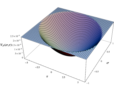
The structure of this $S$- and $T$-stabilizing dS minimum is displayed in Fig. 3. Finally, let us calculate the F-terms in the 2 sectors of the model and the gravitino mass to get a feeling for the supersymmetry breaking occurring here. We have

$$m_{3/2}=\langle e^{K/2}|W|\rangle\approx 3\cdot 10^{-2}$$ (21)

and for the F-terms we get

$$F_{T}=\langle e^{K/2}D_{T}W\rangle\approx 10^{-3}\;,\;F_{S}=\langle e^{K/2}D_{S}W\rangle\approx 3\cdot 10^{-4}\;\;.$$ (22)

Thus, supersymmetry is predominantly broken in the $T$-sector which fits into the former result that the minimum for $S$ is nearly supersymmetric. Let us note here the high supersymmetry breaking scale with a gravitino mass of the order of the GUT scale. This is a generic feature of the construction since there is no suppression of the magnitude of $W_{0}$ as compared with the KKLT construction. In addition, lowering $m_{3/2}$ would require tuning $\hat{\cal V}$ to ever larger values which is done by tuning $a$ smaller and $S$ larger - by fluxes which is, however, limited by the upper bound the flux size in type IIB.

Note further, that here the combination of perturbative and non-perturbative effects succeed to stabilize $S$ and $T$ in a true minimum without the presence of any complex structure modulus. This is different from the case studied, e.g., in [63] where upon using only non-perturbative effects tachyonic directions were found in the absence of complex structure moduli (for a more recent argument in favor of the generic stability of the KKLT vacua see [64]).

4.2 Complex structure

We shall now shortly discuss the inclusion of the complex structure moduli (of which the quintic example contains 101). The crucial point here is to note that the flux stabilization of the $U^{\alpha}$-fields will not be significantly influenced by the $\alpha^{\prime}$-correction of the $S$-$T$-sector since the inverse of the Kähler metric decouples the $U^{\alpha}$ from $S$ and $T$. From

$$K=\underbrace{-2\ln(\hat{\cal V}+\hat{\xi}/2)-\ln(S+\bar{S})}_{K_{1}}\underbrace{-\ln(-i\int_{\rm CY_{3}}\bar{\Omega}\wedge\Omega)}_{K_{c.s.}}\Rightarrow K_{a\alpha}=0$$ (23)

we see immediately that the inverse of the Kähler metric must be block diagonal and thus of the form

$$K^{A\bar{B}}=\left(\begin{array}[]{cc}K_{1}^{a\bar{b}}&0\\ 0&K_{c.s.}^{\alpha\bar{\beta}}\end{array}\right)$$ (24)

where $K_{1}^{a\bar{b}}$ is given by eq. (9). The only place where the $S$-$T$-sector can influence the complex structure moduli is through $W$ itself. However, $W$ appears suppressed by $K_{U^{\alpha}}$ in the supercovariant derivative $D_{\alpha}W$ and thus for sufficiently large ${\rm Re}\,U^{\alpha}$ the solution to $D_{\alpha}W=0$ should give an excellent approximation to the true minimum of $U^{\alpha}$.

For the sake of explicitness we take now the simplified case of one complex structure modulus $U=U_{r}+i\cdot\nu$. Then we have (see e.g. [65])

$$K_{c.s.}=-\ln(U+\bar{U})$$ (25)

and it remains to specify the flux superpotential for $U$. Since this is not known for the example of the quintic, we take guidance in toroidal orientifold examples of Lüst et al. [65] where for those with just one complex structure modulus one can write $W_{0}$ as

$$W_{0}=c_{1}+d_{1}\cdot U-(c_{2}+d_{2}\cdot U)\cdot S\;\;.$$ (26)

Here $c_{1},d_{1},c_{2},d_{2}$ are now true constants determined entirely by topological information of the Calabi-Yau.

Figure 4: The F-term scalar potential $V_{F}(S,U)$ at $T=T_{\rm min}\approx 32.8$ leading to a dS minimum at $S\approx 7.9$ and $U\approx 1.9$. The flux parameters are chosen to be $c_{1}=-6.93$, $c_{2}=0.7$, $d_{1}=-3.46$, $d_{2}=0.35$ while all other parameters remain as they were chosen for the quintic in the previous subsection.

The inverse Kähler metric is now

$$K^{A\bar{B}}=\left(\begin{array}[]{cc}K_{1}^{a\bar{b}}&0\\ 0&(U+\bar{U})^{2}\end{array}\right)$$ (27)

and we get the scalar potential

$$V_{F}(S,T,U) = e^{K}\,\left\{K^{T\bar{T}}[W_{T}\overline{W_{T}}+(W_{T}\cdot\overline{WK_{T}}+c.c.)]\right.$$ (28)

$$\;\left.+[K^{T\bar{S}}D_{T}W\overline{D_{S}W}+c.c]+K^{S\bar{S}}|D_{S}W|^{2}+K^{U\bar{U}}|D_{U}W|^{2}\right.$$

$$\left.+3\hat{\xi}\,\frac{\hat{\xi}^{2}+7\hat{\xi}\hat{\cal V}+\hat{\cal V}^{2}}{(\hat{\cal V}-\hat{\xi})(\hat{\xi}+2\hat{\cal V})^{2}}\,|W|^{2}\right\}\;\;.$$

The supersymmetric stationary points for $S$ and $U$ are now given by

$$S_{0}=-\,\frac{c_{1}+d_{1}\,U_{0}}{c_{2}+d_{2}\,U_{0}}=-\,\frac{d_{1}}{d_{2}}\;,\;U_{0}=\frac{c_{1}}{d_{1}}=\frac{c_{2}}{d_{2}}\;\;.$$ (29)

Here we neglected the contribution $\langle A\exp(-aT)\rangle\sim 0.1$ do to its smallness. Guided by this, a choice of flux parameters

$$c_{1}=-6.93\;,\;c_{2}=0.7\;,\;d_{1}=-3.46\;,\;d_{2}=0.35$$ (30)

should again lead to $S\approx S_{0}=9.8$ and now also $U\approx U_{0}=2$ while giving a $W_{0}$ of the same size as in the previous subsection for the above values of $S$ and $U$. In using the fractional numbers for the constants $c_{1},c_{2},d_{1},d_{2}$ we were borrowing from the fact that in the many complex structure moduli case (as realized on the quintic) the 3-form flux supported on the many different 3-cycles allows for tuning the constants the same way as the total $W_{0}$ is tuned to get the cosmological constant small.

The analysis of the scalar potential eq. (28) reveals a true minimum at

$$T_{r}\approx 32.8\;,\;S_{r}\approx 7.9\;,\;U_{r}\approx 1.9\;\;.$$ (31)

This stationary point is again a minimum as seen from the masses

$$m_{U_{r}}^{2} \approx 3\cdot 10^{-5}\;,\;m_{S_{r}}^{2}\approx 3\cdot 10^{-6}\;,\;m_{T_{r}}^{2}\approx 1.5\cdot 10^{-8}$$

$$m_{\nu}^{2} \approx 3\cdot 10^{-5}\;,\;m_{\sigma}^{2}\approx 10^{-6}\;,\;m_{\tau}^{2}\approx 4\cdot 10^{-8}\;\;.$$ (32)

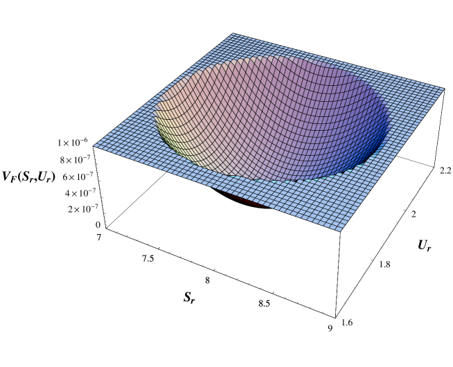
It is de Sitter and looks practically unchanged with respect to $S$ and $T$. The axions of $T$ and $S$ remain stabilized at $\tau=\sigma=0$ as before and it is clear that the axion of $U$ is fixed at $\nu=0$ the same way as $\sigma$ since they enter $W$ in the same way. Fig. 4 displays the minimum for the real parts of $S$ and $U$.

A property of both the $S$-$T$-$U$-model presented here and the $S$-$T$-model of the last subsection is that the volume modulus $T_{r}$ remains to be the lightest field after stabilization.

Note that $U_{r}$ deviates by less than 5% from its supersymmetric stationary point. This fits with the result for the F-terms in the different sectors

$$F_{T}\approx 7\cdot 10^{-4}\;,\;F_{S}\approx 2\cdot 10^{-4}\;,\;F_{U}\approx 9\cdot 10^{-5}$$ (33)

which again shows the dominance of the $T$-sector SUSY breaking as well as that SUSY is most weakly broken in the $U$-sector. The gravitino mass is

$$m_{3/2}\approx 10^{-2}\;\;.$$ (34)

The smallness of the deviation which $U$ has compared with its SUSY stationary point makes it possible to check the numerical results with an analytic expansion of the solution for $U$ away from the SUSY point $U_{0}$ in terms of powers of $\hat{\xi}/(2\hat{\cal V})\approx 0.03$. We use here a method developed in [66] which works as follows: Take the scalar potential for $U$, plug in an expansion $U=U_{0}\cdot(1+a_{1}\frac{\hat{\xi}}{2\hat{\cal V}}+\ldots)$ and determine the perturbed stationary point in $U$ by determining the coefficient $a_{1}$ from $\partial_{a_{1}}V_{F}(U)=0$. Following this recipe we arrive at an expression for the first expansion coefficient

$$a_{1}=-\left\langle 4A\,e^{-aT_{r}}\gamma\,\left(\frac{T_{r}}{S_{r}}\right)^{3/2}\cdot{\cal O}(1)\right\rangle\approx-1.67\;\;.$$ (35)

If we plug this result back into the expansion of $U$ around $U_{0}$ we get

$$U=U_{0}\left(1+a_{1}\frac{\hat{\xi}}{2\hat{\cal V}}\right)\approx 1.91$$ (36)

which agrees with the full numerical solution up to 1% and thus shows the reliability of the numerical result.

We discussed here the case of one complex structure modulus explicitly. However, the example used here, the Calabi-Yau given by the quintic hypersurface $C\mathbb{P}^{4}_{1,1,1,1,1}$, has $h^{2,1}=101$ complex structure moduli. The stabilization of all of them cannot be done explicitly in a practically feasible way. However, since all complex structure moduli enter the flux superpotential in the qualitatively the same way as the first one discussed above, and for this first one the SUSY condition $D_{U}W=0$ gives a rather good approximation for its minimum, the stabilization of several complex structure moduli should proceed without major changes along the lines of [6].

Hence, it seems to be reasonably safe to conclude that this construction stabilizes all geometric moduli in a candidate string example given by $C\mathbb{P}^{4}_{1,1,1,1,1}$ explicitly in a tunable dS vacuum at parametrically large volume and weak string coupling.

4.3 Application to all smooth hypersurfaces in $C\mathbb{P}^{4}$ with $h^{1,1}=1$

We shall now try to extend the results of the previous section to other Calabi-Yau 3-folds than $C\mathbb{P}^{4}_{1,1,1,1,1}$. To carry over as much of the structure as possible, we restrict ourselves to the case $h^{1,1}=1$ although there are no reasons of principle which should prevent us from extending the construction to $h^{1,1}>1$, too (for instance, it should be rather straightforward to apply our construction to the $C\mathbb{P}^{4}_{1,1,1,6,9}$-model of [58]). There are three other non-singular hypersurfaces in projective 4-space $C\mathbb{R}^{4}$ which yield a Calabi-Yau 3-fold with $h^{1,1}=1$ besides $C\mathbb{P}^{4}_{1,1,1,1,1}$. We list in Table 1 the four manifolds and their relevant properties for comparison [67].

	$C\mathbb{P}^{4}_{1,1,1,1,1}$	$C\mathbb{P}^{4}_{2,1,1,1,1}$	$C\mathbb{P}^{4}_{4,1,1,1,1}$	$C\mathbb{P}^{4}_{5,2,1,1,1}$
$h^{2,1}$	101	103	149	145
$\chi$	-200	-204	-296	-288
$\kappa$	5	3	2	1

Table 1: quintic hypersurfaces in $C\mathbb{P}^{4}$

From this synopsis it is clear that all four Calabi-Yau 3-folds satisfy the necessary requirement $h^{2,1}>h^{1,1}$ to be eligible for the procedure of moduli stabilization with Kähler uplifting from the preceding sections. In particular, the results for $C\mathbb{P}^{4}_{1,1,1,1,1}$ should carry over nearly unchanged to $C\mathbb{P}^{4}_{2,1,1,1,1}$ as there $\chi$ is practically the same. The smaller value of the self intersection $\kappa$ on $C\mathbb{P}^{4}_{2,1,1,1,1}$ will require us to stabilize the dilaton at even weaker string coupling compared to the former case of $C\mathbb{P}^{4}_{1,1,1,1,1}$ in order to maintain the same minimum for $T$. The other two possibilities will require stabilizing the dilaton at a relatively stronger string coupling as there the Euler numbers are about 40-50% larger in size.

5 Conclusion

In this paper we discussed (building on an earlier analysis by [54]) de Sitter vacua in string theory which arise by spontaneously breaking supersymmetry through F-terms induced by the leading quantum correction to the Kähler potential of the Kähler moduli. This correction arises from the known $R^{4}$-term of type IIB string theory at ${\cal O}(\alpha^{\prime 3})$. Taking into account the dependence of this correction on the dilaton allows us to stabilize both the volume Kähler modulus and the dilaton in a metastable dS minimum which is at parametrically large volume of ${\cal O}(100)$ and weak string coupling $g_{S}\sim 0.1$. In addition, we are able to take the interplay between the leading non-perturbative contribution to the superpotential and the leading perturbative Kähler correction into a regime where both are ${\cal O}(0.1)$ or even smaller. Hence, these dS minima are reliable as both the perturbative $\alpha^{\prime}$-expansion and the non-perturbative expansion in the superpotential are under parametrical control. It is crucial here, that in type IIB the back-reaction of fluxes of $(1,2)$- and $(0,3)$-type is confined to changes in the warp factor. This, in turn allows us to make the $\alpha^{\prime}$-expansion parameter small by trading its size for that of the flux superpotential.

Let us note here, that the bound on the size of 3-form flux and thus the size of $W_{0}$ in type IIB [68] may prevent us from getting exponentially large volumes: Should the limit on flux size also yield a lower bound of $g_{S}$, then this limits the maximal rank of the gauge groups in the non-perturbative sector usable for tuning the volume to large values. The gauge group rank, however, sets the scale of the achievable volume, which thus can be exponentially large only if the rank can be made very large and $g_{S}$ very small.

As the vacuum value of the superpotential in these vacua is generically ${\cal O}(1\ldots 10)$, any non-exponentially small lower bound on $g_{S}$ in type IIB flux compactifications would imply a necessarily high-scale gravitino mass and supersymmetry breaking scale. In the examples discussed, we get typical values of $m_{3/2}\sim 10^{-3}\ldots 10^{-2}$.

In the next step we included the stabilization of a single complex structure modulus by fluxes explicitly. Since it turns out that this modulus remains stabilized at values very close to the one dictated by the supersymmetry condition in the complex structure moduli sector, this implies that the stabilization of several complex structure moduli is straight forward along the general procedure of type IIB flux compactifications. This feature allows us to conclude that the vacua constructed apply directly to a sub-class of type IIB flux compactifications on Calabi-Yau 3-folds with $h^{1,1}=1$ which is given by the quintic hypersurfaces in projective 4-space $C\mathbb{P}^{4}$. Extending the construction to the case $h^{1,1}>1$ should be straightforward.

All four members of this class ($C\mathbb{P}^{4}_{1,1,1,1,1}$, $C\mathbb{P}^{4}_{2,1,1,1,1}$, $C\mathbb{P}^{4}_{4,1,1,1,1}$, $C\mathbb{P}^{4}_{5,2,1,1,1}$) satisfy the requirements of the construction, namely that $h^{2,1}>h^{1,1}$. Furthermore, the effects used are reasonably sound effects of string theory corroborated by solid string calculations (especially the ${\cal O}(\alpha^{\prime 3})$-correction). Viewed together, this gives an explicit construction of dS vacua in string theory which stabilize all geometric moduli in these four examples.

Interesting cosmological questions arise now in these models. Since the cosmological constant of these dS vacua is amenable to fine-tuning by the fluxes, one may want to look for realizations of inflation in this scenario. Here one may revisit, e.g., the mechanism of inflation driven by open string $D3$-$\overline{D3}$-distance modulus [69] or axionic directions of the closed string moduli potential along the lines of [70, 55, 71, 72], which is however left for future work.

Let us finally mention, that it may be useful to revisit the question of stabilizing the dilaton by a combination of $H_{(3)}$-flux and gaugino condensation in the heterotic string [73], since there the $R^{4}$-term corrects the Kähler potential of the heterotic dilaton [74]. As in the models discussed here, there is no need to have $|W_{0}|$ small while we get large values for $T$. This could translate in the heterotic case into a viable way to stabilize the dilaton at the phenomenologically required value $S\sim 2$ with having a flux superpotential of ${\cal O}(1)$ as required there by flux quantization.