Universality From Very General Nonperturbative Flow Equations in QCD

Abstract

In the context of very general exact renormalization groups, it will be shown that, given a vertex expansion of the Wilsonian effective action, remarkable progress can be made without making any approximations. Working in QCD we will derive, in a manifestly gauge invariant way, an exact diagrammatic expression for the expectation value of an arbitrary gauge invariant operator, in which many of the non-universal details of the setup do not explicitly appear. This provides a new starting point for attacking nonperturbative problems.

In this paper, we will describe a major development in the understanding of how a manifestly gauge invariant approach to QCD, based on the exact renormalization group (ERG) ERG , may be used as a practical tool for extracting nonperturbative information.

Given some field theory, the basic idea of the ERG (for reviews see Reviews ; TRM-elements ; Pawlowski:2005xe ) is the implementation of a momentum cutoff, $\Lambda$, in such a way that the physics at this scale is described in terms of parameters relevant to this scale. The effects of the modes above $\Lambda$, which have been integrated out, are encoded in the Wilsonian effective action, $S_{\Lambda}$. The ERG (or flow) equation determines how $S_{\Lambda}$ evolves with $\Lambda$, thereby linking physics at different energy scales and so providing access to nonperturbative physics. One of the great benefits of the ERG approach is that renormalization is built in: solutions to the flow equation, from which physics can be extracted, are naturally phrased directly in terms of renormalized parameters.

Compared to alternative ERG approaches to QCD (for a comprehensive review of these, see Pawlowski:2005xe ), the manifestly gauge invariant approach advocated by this paper has both a major advantage and a major disadvantage. The benefit of the formalism is that gauge invariance is manifestly preserved along the entire flow: not only are the Ward-Takahashi Identities (WTIs) not modified (as is generically the case), but they are in fact particularly simple as a consequence of the exact preservation of gauge invariance. The drawback of the approach is that the implementation of a manifestly gauge invariant ERG ymi ; aprop ; mgierg1 ; QCD requires considerable complication. A pressing question for this manifestly gauge invariant approach, then, is whether the complications can be reduced to a level where the elegance and power of manifest gauge invariance provides a real, practical advantage.

Already, there have been tantalizing hints that this might be possible, as evidenced by the surprisingly high degree of universality found at intermediate stages of perturbative computations of $\beta$ function coefficients mgierg1 ; mgierg2 ; RG2005 ; mgiuc ; QCD and expectation values of gauge invariant operators evalues . By this, we mean the following. The complications arising in the implementation of a manifestly gauge invariant ERG reside in the regularization and suitable generality of the way in which the high energy modes are integrated out; as such, the complications amount to nonuniversal details of which physical observables must be independent. Now, despite both the $\beta$ function and the expectation values of generic gauge invariant operators being scheme dependent it is found that many (though of course not all) of the explicit nonuniversalities nevertheless cancel out, to all orders in perturbation theory. In this paper, we will show how these cancellations can be extended nonperturbatively, which represents a crucial first step in understanding how to practically use this formalism for nonperturbative calculations.

We now illustrate these considerations in the context of expectation values of gauge invariant operators, whose flow can be computed by taking the ERG equation and considering linear, gauge invariant perturbations to the Wilsonian effective action evalues . Thus, having inserted a gauge invariant operator, $\mathcal{O}$, at the bare scale, we can track its evolution as we integrate out degrees of freedom. In the limit that all fluctuations have been integrated out, the value of this (effective) operator, $\mathcal{O}_{\Lambda=0}$, simply corresponds to the renormalized expectation value we are seeking to compute:

$$\left\langle\mathcal{O}\right\rangle_{R}=\mathcal{O}_{\Lambda=0}.$$ (1)

In evalues , a manifestly gauge invariant, perturbative expression for the $n$-loop contribution to the field independent part of $\mathcal{O}_{\Lambda}$—which is the only contribution that survives the limit $\Lambda\rightarrow 0$—, $g^{2(n-1)}\mathcal{O}_{n}$, was derived, such that

$$\frac{d}{d\Lambda}\sum_{n}\left[g^{2(n-1)}\mathcal{O}_{n}\right]=\frac{d}{d\Lambda}\sum_{n}\left[g^{2(n-1)}\bar{{\cal Q}}_{n}\right],$$ (2)

where $\bar{{\cal Q}}_{n}$ is a set of $n$-loop ERG diagrams. The expression (2) can be directly integrated and so we see that the perturbative contributions to $\left\langle\mathcal{O}\right\rangle_{R}$ are given by sets of terms evaluated at the bare scale, and sets of terms evaluated at $\Lambda=0$. In the perturbative treatment, the latter terms in fact vanish evalues and so $\left\langle\mathcal{O}\right\rangle_{R}$ can be expressed solely as contributions directly fixed by the boundary condition at the bare scale (at the very end of a calculation, the bare scale is tuned to infinity, which essentially corresponds to taking the continuum limit TRM-elements ).

Now, the set of diagrams contributing to (2) exhibit a strong degree of universality, in the sense that many of the nonuniversal details of the setup do not explicitly appear (there is, of course, still some scheme dependence present, as should be expected). To understand this statement better, we now review the nonuniversalities inherent in our ERG approach and discuss how they generically cancel out.

One of the key ingredients of any flow equation is that the partition function (and hence the physics derived from it) is invariant under the flow. As a consequence of this, the family of flow equations for some generic fields, $\varphi$, follows from jose

$$-\Lambda\partial_{\Lambda}\,{\rm e}^{\displaystyle-S[\varphi]}=\int_{x}\frac{\delta}{\delta\varphi(x)}\left(\Psi_{x}[\varphi]\,{\rm e}^{\displaystyle-S[\varphi]}\right),$$ (3)

where the $\Lambda$ derivative is performed at constant $\varphi$, any Lorentz indices etc. have been suppressed and we have written $S_{\Lambda}$ as just $S$. The total derivative on the right-hand side ensures that the partition function $Z=\int\mathcal{D}\varphi\,\!\,{\rm e}^{\displaystyle-S}$ is invariant under the flow.

The primary source of nonuniversal details is $\Psi$, which parametrizes (the continuum version of a) general Kadanoff blocking Kadanoff in the continuum, and for which we take the following form mgierg1 :

$$\Psi_{x}=\frac{1}{2}\{\dot{\Delta}^{\varphi\varphi}(x,y)\}\frac{\delta\Sigma}{\delta\varphi(y)},$$ (4)

where it is understood that we sum over all the elements of the set of fields $\varphi$. We now describe each of the components on the right-hand side of (4). First, there are the ERG kernels, $\dot{\Delta}^{\varphi\varphi}$, which are generally different for each of the elements of $\varphi$. Each kernel incorporates a cutoff function which provides ultraviolet (UV) regularization. The notation $\{\dot{\Delta}\}$ denotes a covariantization of the kernel which may be necessary, depending on the symmetries of the theory. Indeed, it is apparent from (3) and (4) that the kernel essentially ties together two functional derivatives at points $x$ and $y$; in gauge theory, we can covariantize this statement by using e.g. straight Wilson lines between these two points. In practice, we leave the covariantization unspecified, demanding only that it satisfies general requirements ymi ; mgierg1 . The remaining ingredient in (4) is $\Sigma\equiv S-2\hat{S}$, where $\hat{S}$ is the seed action mgierg1 ; mgierg2 ; seed : a functional with the same symmetries as the Wilsonian effective action which partially parametrizes how modes are integrated out along the flow.

The other source of nonuniversality in (3) is more subtle: it might be necessary to include some unphysical regulator fields in the set $\varphi$. Indeed, this is precisely the case in the manifestly gauge invariant ERG formulation of QCD that we employ, where covariantization of the cutoff functions is not sufficient to completely regularize the theory. To furnish a complete regularization of QCD we embed the physical theory into a spontaneously broken $\mathrm{SU}(N|N)$ gauge theory, with the unphysical fields supplying precisely the necessary extra regularization sunn ; QCD .

Substituting (4) into (3) we perform the $\Lambda$-derivative on the left-hand side. Identifying terms with the same number of fields on both sides allows us to write down a flow equation for the vertex coefficient functions of the Wilsonian effective action (i.e. the fields themselves and any symmetry factors have been stripped off). Anticipating specialization to QCD, we recall that, in this case, it is convenient to scale the coupling out of the covariant derivative ymi . This has the effect of causing $S\rightarrow S/g^{2}$ and so we make the replacement $\Sigma\rightarrow\Sigma_{g}\equiv g^{2}S-2\hat{S}$. The flow equation for QCD is shown in figure 1 QCD .

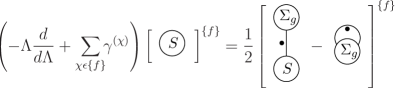
Figure 1: The diagrammatic form of the QCD flow equation for vertices of the Wilsonian effective action.

The first term on the left-hand side represents the flow of all independent Wilsonian effective action vertex coefficient functions corresponding to the set of fields, $\{f\}$. Our notation is slightly different to previous works for later clarity: since the $\Lambda$-derivative strikes just a vertex coefficient function—all fields having been stripped off—we need not write this as a partial derivative with fields held constant (cf. (3)). The term $\sum_{\chi\epsilon\{f\}}\gamma^{(\chi)}$ explicitly takes account of the anomalous dimensions of the fields which suffer field strength renormalization. The field $\chi$ belongs to the set of fields $\{f\}$ and the notation $\gamma^{(\chi)}$ just stands for the anomalous dimension of the field $\chi$ (which is zero for all but the components of the superfields into which the physical quark fields are embedded QCD ).

The lobes on the right-hand side of the flow equation are vertex coefficient functions of $S$ and $\Sigma_{g}$. These lobes are joined together by vertices of the covariantized ERG kernels, denoted by $\stackrel{{\scriptstyle\bullet}}{{\mbox{\rule{28.45274pt}{0.56905pt}}}}$, which, like the action vertices, can be decorated by fields belonging to $\{f\}$. The rule for decorating the diagrams on the right-hand side is simple: the set of fields, $\{f\}$, are distributed in all independent ways between the component objects of each diagram. Embedded within the diagrammatic rules is a prescription for evaluating the group theory factors, for which the reader is referred to mgierg1 .

Now, returning to (2), it is the case that the set of diagrams on the right-hand side contains no explicit dependence on either the seed action or the details of the covariantization of the kernels. Before stating what the right-hand side does depend on, we describe the procedure by which the aforementioned nonuniversal details cancel out. The key is to utilize the (perturbative) diagrammatic calculus, proposed in aprop , refined in mgierg1 ; RG2005 and completed in mgiuc .

The central ingredient to this calculus is the ‘effective propagator relation’ aprop ; mgierg1 ; seed , which arises as follows. First, we perform a perturbative expansion of the actions and flow equation. Secondly, we turn the freedom inherent in the seed action to our advantage by setting the seed action classical, two-point vertices equal to their Wilsonian effective action counterparts. It then follows, from the classical part of the flow equation, that sets of these vertices are related to sets of kernels according to:

$$S_{0MR}^{\ \;\varphi\;\varphi}(p)\Delta^{\,\varphi\,\varphi}_{RN}(p^{2}/\Lambda^{2})=\delta_{MN}-p^{\prime}_{M}p_{N},$$ (5)

where it is understood that we sum not only over the index, $R$, but also over the elements of $\varphi$ which carry this index. $S_{0MR}^{\ \;\varphi\;\varphi}(p)$ is a classical, two-point vertex carrying indices $M$ and $R$ and momenta $p_{\mu}$ and $-p_{\rho}$. $\Delta^{\,\varphi\,\varphi}_{RN}(p^{2}/\Lambda^{2})$ is an integrated kernel a.k.a. effective propagator

$$\stackrel{{\scriptstyle\bullet}}{{\Delta}}\equiv-\Lambda\partial_{\Lambda}\Delta,$$

where the $\Lambda$-derivative is performed with any dimensionless couplings on which $\Delta$ depends held constant mgierg1 ; mgierg2 ; QCD . On the right-hand side of (5) there is a Kronecker-$\delta$ function and a remainder term comprising a function of $p_{\mu}$, $p^{\prime}_{M}$, and a function of $p_{\nu}$, $p_{N}$. In QCD, these functions are non-null in the gauge sector (which we recall is extended due to the embedding into $\mathrm{SU}(N|N)$). For this reason, the remainders are referred to as ‘gauge remainders’. As an example, in the physical gauge sector—which has gauge field $A^{1}_{\mu}$—, the relationship (5) is

$$S^{\ A^{1}A^{1}}_{0\mu\ \;\alpha}(p)\Delta^{A^{1}A^{1}}_{\alpha\ \,\nu}(p)=\delta_{\mu\nu}-\frac{p_{\mu}}{p^{2}}p_{\nu}.$$

From this we see that the effective propagator is the inverse of the classical, two-point vertex only in the transverse space. It is important to note that the effective propagators are by no means propagators in the usual sense; indeed, they cannot be, since we have not fixed the gauge. However, they have a similar form and play a similar diagrammatic role, and so the terminology ‘effective propagator’ is intuitively helpful. The components of the gauge remainder are identified as follows: $p^{\prime}_{M}=p_{\mu}/p^{2}$, $p_{N}=p_{\nu}$.

Equation (5) has a very useful diagrammatic representation, shown below:

We have attached the effective propagator, denoted by a solid line, to an arbitrary structure since it only ever appears as an internal line. The field labeled by $M$ can be any of the physical or regulator fields. The object $\begin{array}[]{c}\includegraphics{GR.eps}\end{array}\!\!\equiv\;>\!\!\!\rhd$ is a gauge remainder. Recalling (5), we identify $>$ with $p^{\prime}_{M}$ and $\rhd$ with $p_{N}$.

The reason that the effective propagator relation is so useful is that it allows diagrams to be simplified: in any term where a classical, two-point vertex is attached to an effective propagator, we can collapse this structure down to Kronecker-$\delta$ and a gauge remainder. When deriving (2) we find that the diagrams formed by the Kronecker-$\delta$ contribution cancel against other terms. This leaves the diagrams containing gauge remainders, which it turns out can be further processed by using the WTIs ymi ; aprop ; mgierg1 . In a subset of the resulting diagrams the effective propagator relation can again be applied. Iterating the procedure, we find that all explicit dependence on the seed action and details of the covariantization of the kernels cancels out. When the dust has settled, the set of diagrams contributing to $\left\langle\mathcal{O}\right\rangle_{R}$ comprise only four ingredients, the first three of which are vertices of $\mathcal{O}_{\Lambda}$, effective propagators and instances of the gauge remainder component $>$. The final ingredient is vertices of the Wilsonian effective action, but where none of these are classical, two-point vertices. This is because all such terms have been removed by application of the effective propagator relation. This has led us, in the past RG2005 ; mgiuc , to introduce reduced vertices, defined as follows: given the loop expansion of a Wilsonian effective action (or seed action) vertex with an arbitrary number of legs we subtract off the classical, two-point component.

The major breakthrough of this paper is the realization that the diagrammatic calculus has a non-perturbative extension. The apparent barrier to this is that the effective propagator relation and the reduction of the Wilsonian effective action vertices are apparently rooted in perturbation theory, since both involve the introduction and utilization of classical vertices. The solution to this problem is as simple as it is obvious: we define a set of two-point vertices $(\Delta^{\!-1})^{\,\varphi\,\varphi}_{S\,T}(p)$, such that

$$(\Delta^{\!-1})^{\;\varphi\;\varphi}_{MR}(p)\Delta^{\,\varphi\,\varphi}_{RN}(p^{2}/\Lambda^{2})=\delta_{MN}-p^{\prime}_{M}p_{N}.$$ (6)

Clearly, $(\Delta^{\!-1})^{\;\varphi\;\varphi}_{MR}(p)$ is just numerically equal to $S_{0MR}^{\ \;\varphi\;\varphi}(p)$, but it makes sense to isolate any instances of $(\Delta^{\!-1})^{\;\varphi\;\varphi}_{MR}(p)$ in action vertices even when no loop expansion has been performed. Essentially, all we have done is change notation to emphasise that the objects of which the integrated kernels are the inverses (in the appropriate space) can be introduced independently of performing a perturbative expansion. This subtle shift of perspective holds the key to extending the diagrammatic calculus nonperturbatively. The complimentary part of this strategy is to generalize the reduction of action vertices according to:

$$\leavevmode\resizebox{113.81102pt}{}{\includegraphics{RWEA.epsi}},\ \leavevmode\resizebox{113.81102pt}{}{\includegraphics{RSA.epsi}},$$

where it is understood that the vertex with argument $\Delta^{\!-1}$ is null unless the number of fields in the set $\{f\}$ is precisely equal to two. In the weak coupling limit, these definitions just reduce to those of RG2005 ; mgiuc : namely that a reduced vertex does not possess a classical, two-point component.

Remarkably, the introduction of the set of vertices, $(\Delta^{\!-1})^{\,\varphi\,\varphi}_{S\,T}(p)$, together with the generalization of the reduced vertices are the only steps necessary to apply the diagrammatic calculus nonperturbatively. Thus, it turns out that we can write, exactly,

$$\frac{d\mathcal{O}}{d\Lambda}=\frac{d\bar{{\cal Q}}}{d\Lambda},$$ (7)

where we take $\mathcal{O}$ to represent the field independent part of $\mathcal{O}_{\Lambda}$. The set of diagrams, $\bar{{\cal Q}}$, is given by

$$\bar{{\cal Q}}\equiv-2\sum_{s=1}^{\infty}\sum_{m=0}^{2s-1}\sum_{j=0}^{s}\frac{\Upsilon_{s,j}}{m!}g^{2s}\left[\begin{array}[]{c}\vspace{1ex}\begin{array}[]{c}\begin{picture}(1.0,1.0)(0.0,0.0)\put(0.0,0.0){\framebox(1.0,1.0)[]{$\,\mathcal{O}\,$}} \end{picture}\end{array}\\ \left[\begin{array}[]{c}\includegraphics{ReducedWEA.epsi}\end{array}\right]^{j}\end{array}\right]^{\Delta^{s}>^{m}},$$ (8)

with, for non-negative integers $a$ and $b$, the definition

$$\Upsilon_{a,b}\equiv\frac{(-1)^{b+1}}{a!b!}\left(\frac{1}{2}\right)^{a+1}.$$

We understand the notation of (8) as follows. The diagrammatic function $\bar{{\cal Q}}$ stands for all connected diagrams which can be created from a single vertex of $\mathcal{O}_{\Lambda}$ (with any number of legs), $j$ reduced Wilsonian effective action vertices (each with any number of legs), $s$ effective propagators and $m$ of the gauge remainder components, $>$. For the rules specifying how to explicitly construct fully fleshed out diagrams contributing to $\bar{{\cal Q}}$ see mgiuc ; RG2005 . Notice that the overall $g$ dependence of $\bar{{\cal Q}}$ comes not just from the factor of $g^{2s}$ sitting in front of the sum over diagrams but also from the vertices of both $\mathcal{O}_{\Lambda}$ and the Wilsonian effective action; this is crucial as it is the nonperturbative contributions to these vertices which will provide the nonperturbative contributions to $\bar{{\cal Q}}$.

Again, we integrate (7) between $\Lambda=0$ and the bare scale. The latter contributions, for which the coupling is small, contain the perturbative contributions, (2), and additional, nonperturbative parts, arising from the fact that the vertices appearing in $\bar{{\cal Q}}$ are exact. The investigation of these contributions is left to the future; similarly, we defer answering the question as to whether the contributions from $\Lambda=0$ survive in this nonperturbative formulation. However, we do note that, to answer this, we must find out whether the coupling grows sufficiently fast in the infrared to prevent the $\Lambda=0$ contributions from vanishing evalues . The investigation of this will be greatly helped by the fact that the nonperturbative generalization of the diagrammatic calculus enables us to derive an exact diagrammatic expression for the $\beta$ function, with no explicit dependence on either the seed action, or details of the covariantization of the kernels.

- (1) K. Wilson and J. Kogut, Phys. Rep. 12 C (1974) 75; F. J. Wegner and A. Houghton, Phys. Rev. A 8 (1973) 401; J. Polchinski, Nucl. Phys. B 231 (1984) 269.
- (2) M. E. Fisher, Rev. Mod. Phys. 70 (1998) 653; D. F. Litim and J. M. Pawlowski, in The Exact Renormalization Group, ed A. Krasnitz et al., World Sci (1999) 168; K. Aoki, Int. J. Mod. Phys. B 14 (2000) 1249; J. Berges, N. Tetradis and C. Wetterich, Phys. Rept. 363 (2002) 223; C. Bagnuls and C. Bervillier, Phys. Rept. 348 (2001) 91; J. Polonyi, Central Eur. J. Phys. 1 (2003) 1; M. Salmhofer and C. Honerkamp, Prog. Theor. Phys. 105 (2001) 1; H. Gies, hep-ph/0611146.
- (3) T. R. Morris, Prog. Theor. Phys. Suppl. 131 (1998) 395.
- (4) J. M. Pawlowski, hep-th/0512261.
- (5) T. R. Morris, in The Exact Renormalization Group, ed A. Krasnitz et al., World Sci (1999) 1; T. R. Morris, Nucl. Phys. B 573 (2000) 97; T. R. Morris, JHEP 0012 (2000) 012.
- (6) S. Arnone, A. Gatti and T. R. Morris, Phys. Rev. D 67 (2003) 085003.
- (7) O. J. Rosten, Ph.D. Thesis, hep-th/0506162; S. Arnone, T. R. Morris and O. J. Rosten, hep-th/0507154; S. Arnone, T. R. Morris and O. J. Rosten, hep-th/0606181.
- (8) T. R. Morris and O. J. Rosten, Phys. Rev. D 73 (2006) 065003.
- (9) T. R. Morris and O. J. Rosten, J. Phys. A 39 (2006) 11657.
- (10) O. J. Rosten, J. Phys. A 39 (2006) 8699; J. Phys. A 39 (2006) 8141.
- (11) O. J. Rosten, Int. J. Mod. Phys. A 21 (2006) 4627.
- (12) O. J. Rosten, hep-th/0604183.
- (13) J. I. Latorre and T. R. Morris, JHEP 0011 (2000) 004; Int. J. Mod. Phys. A 16 (2001) 2071.
- (14) L. P. Kadanoff, Physics 2 (1966) 263.
- (15) S. Arnone, A. Gatti and T. R. Morris, JHEP 0205 (2002) 059; S. Arnone, A. Gatti, T. R. Morris and O. J. Rosten, Phys. Rev. D 69 (2004) 065009; S. Arnone, T. R. Morris and O. J. Rosten, JHEP 0510 (2005) 115.
- (16) S. Arnone, Y. A. Kubyshin, T. R. Morris and J. F. Tighe, Int. J. Mod. Phys. A 17 (2002) 2283.