Proof of triviality of $\lambda\phi^{4}$ theory

Abstract

We show that a recent analysis in the strong coupling limit of the $\lambda\phi^{4}$ theory proves that this theory is indeed trivial giving in this limit the expansion of a free quantum field theory. We can get in this way the propagator with the renormalization constant and the renormalized mass. As expected the theory in this limit has the same spectrum as a harmonic oscillator. Some comments about triviality of the Yang-Mills theory in the infrared are also given.

In a series of papers we showed recently that gradient expansions are to be considered as strong coupling expansions when applied to the study of field theory both classical and quantum. In general relativity this gives a sound proof of the so called Belinski, Khalatnikov and Lifshitz conjecture fra1 . Analysis of a classical scalar theory was also given fra2 . Finally, a quantum theory applied to the symmetric phase of a single component $\lambda\phi^{4}$ theory was given fra3 . Application to the $N$-component theories was also proposed fra4 . The main development of these works arises from a paper about duality principle in perturbation theory fra5 .

The quantum formulation of the strong coupling expansion given in fra3 opened up a problem about an almost completely verified property of the $\lambda\phi^{4}$ theory, that is, this theory is trivial in the limit of the coupling going to infinity for dimensionality greater than four zj . This was proved by Aizenman aiz . In four dimensions the problem is still open but results obtained since eighties through some works by Lüscher and Weisz lw1 ; lw2 ; lw3 ; lw4 and Kati and Shen ks1 seem to give a strong indication that this theory is trivial. The present situation in four dimensions is described by Stevenson ste and by Balog, Niedermayer, and Weisz wei with respect to a fit of the propagator requiring more than one term in the free form. In dimension lesser than four the model is expected to be not trivial. Anyhow, it is interesting to note that this property of the scalar theory helped people to give some limits on the mass of the Higgs boson (see e.g. ks2 ). In this case a current view is given in cc1 ; cc2 analyzing data coming from lattice computations.

The point to be emphasized is that one generally assumes that the theory is trivial when the renormalized coupling constant goes to zero in the limit of a large cut-off and the theory becomes a free theory in this limit. This limit coincides with the one where the bare coupling constant goes to infinity, that is the case we discussed analytically in fra3 . Indeed, we would like to consider a redefinition of the triviality of a quantum field theory in the limit of a bare coupling going to infinity. We define “trivial” a theory that has a two-point function in the form

$$G(p)=\sum_{n}\frac{Z_{n}}{p^{2}+m_{n}^{2}-i\epsilon}$$ (1)

that is a weighted sum of free propagators being $Z_{n}$ the weights and $m_{n}$ what we call the spectrum of the theory. This will include also the particular case of all $Z_{n}$ being zero except one. We will prove in the following that for a $\lambda\phi^{4}$ theory this is indeed the case in the limit $\lambda\rightarrow\infty$ and we do the proof by simply summing the series obtained in fra3 .

In our work fra3 we showed that in the limit $\lambda\rightarrow\infty$ the theory has the same spectrum as a harmonic oscillator and this is a strong clue that the theory is trivial in this limit in the sense given above. We will now see that the proof is indeed complete and perturbation theory is consistent with this conclusion. But before we can go on let us give a simple definition through path integrals of a trivial theory for the scalar field. It is well-known that the generating functional for the scalar theory can be written as zj

$$Z[j]=\int[d\phi]e^{\left\{i\int d^{D}x\left[\frac{1}{2}(\partial\phi)^{2}-V(\phi)+j\phi\right]\right\}}$$ (2)

and a free massive theory is given by taking $V(\phi)=\frac{1}{2}\mu_{0}^{2}\phi^{2}$. This means that the above generating functional can be rewritten immediately in a Gaussian form

$$Z[j]=\exp\left[\frac{i}{2}\int d^{D}y_{1}d^{D}y_{2}\frac{\delta}{\delta j(y_{1})}\mu_{0}^{2}\delta^{D}(y_{1}-y_{2})\frac{\delta}{\delta j(y_{2})}\right]Z_{0}[j]$$ (3)

being

$$Z_{0}[j]=\exp\left[\frac{i}{2}\int d^{D}x_{1}d^{D}x_{2}j(x_{1})\Delta(x_{1}-x_{2})j(x_{2})\right]$$ (4)

with $\Delta(x_{1}-x_{2})$ the propagator of the massless theory. This form of the generating functional produces immediately the well-known form of the two-point function $G(p)=1/(p^{2}+\mu_{0}^{2}-i\epsilon)$. So, whenever we are able to rewrite a theory in the above form for the generating functional, that is the Gaussian form

$$Z[j]=\exp\left[\frac{i}{2}\int d^{D}y_{1}d^{D}y_{2}\frac{\delta}{\delta j(y_{1})}A(x_{1})\delta^{D}(y_{1}-y_{2})\frac{\delta}{\delta j(y_{2})}\right]Z_{0}[j]$$ (5)

with $Z_{0}[j]$ defined by some two-point function of the kind $\Delta(p)=\sum_{n}Z_{n}/(p^{2}+m_{n}^{2}-i\epsilon)$ we can immediately write it down the propagator in the form $\Delta(p)=\sum_{n}Z_{n}/(p^{2}+\tilde{A}(p)+m_{n}^{2}-i\epsilon)$. The theory will be proved trivial if the two-point function is indeed a sum of free particle propagators as defined above.

But this is exactly the case for a scalar theory in the limit $\lambda\rightarrow\infty$ as we have already proved that (assuming $\mu_{0}=1$) fra3

$$Z[j]=\exp\left[\frac{i}{2}\int d^{D}y_{1}d^{D}y_{2}\frac{\delta}{\delta j(y_{1})}(-\nabla^{2}+1)\delta^{D}(y_{1}-y_{2})\frac{\delta}{\delta j(y_{2})}\right]Z_{0}[j]$$ (6)

being in this case

$$Z_{0}[j]=\exp\left[\frac{i}{2}\int d^{D}x_{1}d^{D}x_{2}j(x_{1})\Delta(x_{1}-x_{2})j(x_{2})\right]$$ (7)

and

$$\Delta(\omega)=\sum_{n=0}^{\infty}\frac{B_{n}}{\omega^{2}-\omega_{n}^{2}+i\epsilon}$$ (8)

being $K(i)$ the constant

$$K(i)=\int_{0}^{\frac{\pi}{2}}\frac{d\theta}{\sqrt{1+\sin^{2}\theta}}\approx 1.3111028777,$$ (9)

and

$$B_{n}=(2n+1)\frac{\pi^{2}}{K^{2}(i)}\frac{(-1)^{n+1}e^{-(n+\frac{1}{2})\pi}}{1+e^{-(2n+1)\pi}}.$$ (10)

The mass spectrum of the theory is given by

$$\omega_{n}=\left(n+\frac{1}{2}\right)\frac{\pi}{K(i)}\left(\frac{\lambda}{2}\right)^{\frac{1}{4}}$$ (11)

proper to a harmonic oscillator. Now, let us see why in lattice computations the form of the propagator appears to be ks1

$$\Delta(p)=\frac{Z_{R}}{p^{2}+m_{R}^{2}}$$ (12)

being $Z_{R}$ a renormalization constant and $m_{R}$ the renormalized mass. Indeed, higher order corrections in our expansion gives the missing part between the propagator (8) and (12) in the momentum as we showed above. But one has

$$Z_{R}=B_{0}=\frac{\pi^{2}}{K^{2}(i)}\frac{e^{-\frac{\pi}{2}}}{1+e^{-\pi}}\approx 1.144231098$$ (13)

of the order of unit as it should be ks1 . The next terms are exponentially damped, e.g.

$$Z^{\prime}_{R}=B_{1}=\frac{3\pi^{2}}{K^{2}(i)}\frac{e^{-\frac{3\pi}{2}}}{1+e^{-3\pi}}\approx.1483401274$$ (14)

smaller by one magnitude order due to e-folding. The renormalized mass, here given by $\frac{\pi}{2K(i)}\left(\frac{\lambda}{2}\right)^{\frac{1}{4}}$ for $\lambda$ large enough, contributes to damp out higher order terms as it increases with the square of the order making these terms practically not visible on the lattice. So, it would be really interesting to do some computer work to measure them and see all the spectrum of the theory in this limit. We just notice that a strong indication that a further term should be added to the free propagator for the scalar theory in four dimensions, in order to improve the fit to numerical data, has been given in ste ; wei . This further term has a mass being three times the mass of the first term in the symmetric phase in fully agreement with our analysis.

In order to see how our perturbation theory produces terms proper to a trivial theory we push the analysis to second order for the computation of the generating functional. As we will see, no infinite terms appear, rather one gets only the proper momentum contribution. In Ref.fra3 we obtained

$$Z[j]=\left[1-\frac{i}{2}\int\int d^{D}y_{1}(-\nabla^{2}_{y_{1}}+1)\int d^{D}x_{1}d^{D}x_{2}\Delta(y_{1}-x_{1})\Delta(y_{1}-x_{2})j(x_{1})j(x_{2})+\ldots\right]Z_{0}[j].$$ (15)

Now we have to compute the term

$$Z^{(2)}[j] = -\frac{1}{8}\int d^{D}y_{1}d^{D}_{2}\frac{\delta}{\delta j(y_{1})}(-\nabla^{2}+1)\delta^{D}(y_{1}-y_{2})\frac{\delta}{\delta j(y_{2})}\times$$

$$\int d^{D}y_{3}d^{D}y_{4}\frac{\delta}{\delta j(y_{3})}(-\nabla^{2}+1)\delta^{D}(y_{3}-y_{4})\frac{\delta}{\delta j(y_{4})}Z_{0}[j]$$

being $Z_{0}[j]$ given by eq.(7). The computation is very easy to be carried out to give

$$Z^{(2)}[j] = \frac{1}{8}\int d^{D}y_{1}d^{D}y_{2}(-\nabla^{2}_{y_{1}}+1)(-\nabla^{2}_{y_{2}}+1)\times$$

$$\left[i\int d^{D}x_{2}d^{D}x_{3}\Delta(y_{2}-y_{1})\Delta(y_{2}-x_{2})\Delta(y_{1}-x_{3})j(x_{2})j(x_{3})\right.$$

$$+ i\int d^{D}x_{1}d^{D}x_{3}\Delta(y_{2}-x_{1})\Delta(y_{2}-y_{1})\Delta(y_{1}-x_{3})j(x_{1})j(x_{3})$$

$$+ 2i\int d^{D}x_{1}d^{D}x_{2}\Delta(y_{2}-y_{1})\Delta(y_{2}-x_{1})\Delta(y_{1}-x_{2})j(x_{1})j(x_{2})$$

$$- \left.\int d^{D}x_{1}d^{D}x_{2}d^{D}x_{3}d^{D}x_{4}\Delta(y_{2}-x_{1})\Delta(y_{2}-x_{2})\Delta(y_{1}-x_{3})\Delta(y_{1}-x_{4})j(x_{1})j(x_{2})j(x_{3})j(x_{4})\right]\times$$

$$Z_{0}[j].$$

Doing this computation a term appears having the form

$$\frac{1}{4}\int d^{D}y_{1}d^{D}y_{2}[\Delta(y_{2}-y_{1})]^{2}$$ (18)

that seems to diverge. Indeed, when we introduce a cut-off in momentum and take the limit of the cut-off going to infinity, this term is easily proven to be zero. So, we can conclude that our perturbation theory just produces the missing contribution in momentum to the propagator proper to a free theory and the theory is finally shown to be trivial in the limit of the coupling going to infinity. The value of this result relies also on the fact that results from weak perturbation theory that are used for renormalization group analysis, e.g. to compute the beta function in charge renormalization, can also be trusted and all the picture by both sides of perturbation theory appears fully consistent. So, the two-point function of a scalar theory in the limit of the coupling going to infinity has just the simple form of a weighted sum of free propagators with a mass spectrum being the same of a harmonic oscillator.

Finally, we would like to spend a few words about Yang-Mills theory. It is well-known that on a compact manifold the theory has the renormalized coupling going to zero in the infrared cf1 . This result has been reently confirmed notwithstanding the change into the behavior of the propagator cfn . This result seems to translate to the theory on a non-compact manifold through some lattice computations while disagrees with Dyson-Schwinger equation analysis ste2 . So, let us assume as a working hypothesis that both the results on a compact manifold and lattice computations about the running coupling are the one to be trusted. We can conclude that Yang-Mills theory is trivial, in the sense given above, in the infrared limit. This hypothesis has some interesting consequences. Firstly, one can immediately write down the propagator for the gluon

$$D(p)=\sum_{n=0}^{\infty}\frac{Z_{n}}{p^{2}+m_{n}^{2}}$$ (19)

being $Z_{n}$ renormalization constants to be computed, $m_{n}$ the $0^{++}$ glueball mass spectrum that should go as the one of a harmonic oscillator

$$m_{n}=\left(n+\frac{1}{2}\right)\delta$$ (20)

and $\delta/2$ the mass gap of the theory. This in turn will imply that the propagator is finite in the limit of the momentum going to zero and that the scaling law in the infrared for the propagator has the exponent $\kappa=0.5$. Besides, computations on a lattice for the case of 2+1 dimensions also agree with our analysis of a harmonic oscillator spectrum for Yang-Mills theory mck1 ; mck2 . A full accounting of this situation has been presented in fra4 .

In order to analyze further this hypothesis about the Yang-Mills theory, we compare our propagator to the one obtained in the lattice ste2 . To make sense out of this comparison the agreement must be reached after we fix the only free parameter, that is the factor $\delta/2$ into eq.(20). This is the gluon mass. So we take fra4

$$Z_{n}=(2n+1)\frac{\pi^{2}}{K^{2}(i)}\frac{(-1)^{n+1}e^{-(n+\frac{1}{2})\pi}}{1+e^{-(2n+1)\pi}}$$ (21)

and $m_{n}=(2n+1)m_{g}$ being $m_{g}$ the gluon mass to be fitted.

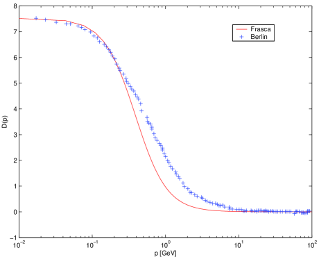
Figure 1: Comparison between lattice gluon propagator and our analytical result.

The result is given in fig.(1) for $m_{g}=389$ MeV. The agreement is excellent supporting our conclusions.

We proved that our approach for strongly coupled quantum field theory applied to a scalar field permits to prove that this theory is trivial in the strong coupling limit. Similar considerations applied to Yang-Mills theory in the infrared permit to obtain some interesting results about the gluon propagator and the mass spectrum of the theory. In this latter case the comparison with lattice results is excellent for a gluon mass of 389 MeV.

- (1) M. Frasca, Int. J. Mod. Phys. D 15, 1373 (2006).
- (2) M. Frasca, hep-th/0509125, to appear in Int. J. Mod. Phys. A.
- (3) M. Frasca, Phys. Rev. D 73, 027701 (2006); Erratum: Phys. Rev. D 73, 049902 (2006).
- (4) M. Frasca, hep-th/0610148, to appear in Int. J. Mod. Phys. A.
- (5) M. Frasca, Phys. Rev. A 58, 3439 (1998).
- (6) J. Zinn-Justin, Quantum Field Theory and Critical Phenomena, (Clarendon Press, 1996) and private communication.
- (7) M. Aizenman, Phys. Rev. Lett. 47, 1 (1981).
- (8) M. Lüscher, P. Weisz, Nucl. Phys. B 290, 25 (1987).
- (9) M. Lüscher, P. Weisz, Nucl. Phys. B 295, 65 (1988).
- (10) M. Lüscher, P. Weisz, Nucl. Phys. B 300, 325 (1988).
- (11) M. Lüscher, P. Weisz, Nucl. Phys. B 318, 705 (1989).
- (12) J. Kuti, Y. Shen, Phys. Rev. Lett. 60, 85 (1988).
- (13) P. M. Stevenson, Nucl. Phys. B 729, 542 (2005).
- (14) J. Balog, F. Niedermayer, P. Weisz, Nucl. Phys. B 741, 390 (2006).
- (15) J. Kuti, L. Lin, Y. Shen, Phys. Rev. Lett. 61, 678 (1988).
- (16) P. Cea, M. Consoli and L. Cosmai, Nucl. Phys. Proc. Suppl. 129, 780 (2004).
- (17) P. Cea, M. Consoli and L. Cosmai, hep-lat/0407024.
- (18) C. S. Fischer, B. Gruter, R. Alkofer, Annals Phys. 321, 1918 (2006).
- (19) C. S. Fischer, A. Maas, J. M. Pawlowski, L. von Smekal, hep-ph/0701050.
- (20) C. S. Fischer, J. Phys. G 32, R253 (2006).
- (21) A.Sternbeck, E.-M.Ilgenfritz, M. Müller-Preussker, A.Schiller, I.L.Bogolubsky, PoS(LAT2006)076.
- (22) B. H. J. McKellar, J. Carlsson, Nucl. Phys. Proc. Suppl. 129-130, 420 (2004).
- (23) B. H. J. McKellar, J. Carlsson, Nucl. Phys. Proc. Suppl. 141, 179 (2005).