DAMTP-2006-114
ITFA-2006-47

Colliding Branes in Heterotic M-Theory
Jean-Luc Lehners^†, Paul McFadden^‡ and Neil Turok^†

^† DAMTP, CMS, Wilberforce Road, CB3 0WA, Cambridge, UK.
^‡ ITFA, Valckenierstraat 65, 1018XE Amsterdam, the Netherlands.

1 Introduction

The riddle of the initial singularity is one of the most basic challenges in cosmology. In standard four-dimensional general relativity, the Riemann curvature diverges at the big bang signalling an irretrievable breakdown of the theory. In higher-dimensional string and M-theory, however, the nature of the initial singularity is significantly altered. Within the higher-dimensional picture, the Riemann curvature may remain bounded all the way to the singularity. In this situation, string and M-theory corrections to the background geometry remain small, allowing one to attempt to study the propagation of strings and branes right up to, and perhaps even across, the singularity.

In this paper, we wish to study such a model of the cosmological background spacetime, within an especially well-motivated theoretical framework. Heterotic M-theory is built on the profound correspondence between supergravity and strongly-coupled heterotic string theory [1, 2], and it remains one of the most promising approaches to the unification of particle physics and gravitation. From the perspective of particle phenomenology, heterotic M-theory makes full use of branes and of the extra M-theory dimension, in order to solve the fundamental puzzles of chirality and of the difference between the GUT and Planck scales. From a cosmological perspective, heterotic M-theory provides a setup in which standard model matter is localised on branes, allowing the background density of such matter to remain finite at the initial singularity.

We consider the collision of two flat, parallel end-of-the-world branes within heterotic M-theory [3, 4]. From the standpoint of the four-dimensional effective theory, this event is a cosmological singularity of the usual catastrophic type. Yet from the higher-dimensional standpoint, the situation is far less singular. The density of standard model matter remains finite. Moreover, even the bulk spacetime between the branes is relatively well-behaved: as we shall show, the Riemann curvature remains finite for all times away from the collision event itself. In the case of trivial, toroidal compactifications of M-theory, this phenomenon is well known. Here, the colliding-brane spacetime is locally flat, a product of two-dimensional compactified Milne space-time, modded out by $\mathbb{Z}_{2}$, with nine-dimensional flat space. At the collision itself, the spacetime is non-Hausdorff since one dimension momentarily disappears. Nevertheless, the low-energy degrees of freedom, described near the collision by winding $M2$ branes (or, equivalently, weakly coupled heterotic strings), possess a regular evolution across the singularity [5].

In more realistic models, six spatial dimensions are compactified on a Calabi-Yau manifold. The dynamics are then described by a five-dimensional effective field theory known as heterotic M-theory, which is a consistent truncation of eleven-dimensional supergravity coupled to the boundary branes [6, 7]. Recently, an improved formulation has been developed which avoids problematic terms involving squares of delta functions [8, 9], giving one greater confidence that classical solutions of the five-dimensional effective theory do indeed provide consistent M-theory backgrounds. In this paper, we shall show that these equations possess a unique global solution representing the collision of two flat end-of-the-world branes which, in the vicinity of the collision, reduces to (2d compactified Milne)/$\mathbb{Z}_{2}\times\mathbb{R}_{3}$, times a finite-volume Calabi-Yau manifold. In this solution, the Riemann curvature is again bounded at all times away from the collision event itself. Our solution offers the intriguing prospect of modelling the big bang as a brane collision in a setup with a high degree of physical realism.

The idea that the big bang was a brane collision in heterotic M-theory was first proposed in [3, 4]. However, the solution representing the approach and collision of two branes has not so far been given in complete form. Important steps towards such a solution were taken by Chamblin and Reall [10], who found a static solution for the bulk geometry in which moving, spatially flat branes can be consistently embedded. The bulk geometry possesses a timelike virtual naked singularity lying ‘beyond’ the negative-tension boundary brane. Two qualitatively different solutions then exist according to whether the boundary branes move through the static bulk in the same, or in opposing, directions. Both of these solutions, together with their time-reverses, are naturally combined within our global solution. In a more recent paper [11], Chen et al. considered the solution where both the positive- and negative-tension boundary branes move towards the virtual singularity. They found an exact solution in a convenient alternative coordinate system which is comoving with the branes. However, Chen et al. found that both branes encounter the naked singularity, resulting in the annihilation of the entire spacetime.

In this paper, we shall argue for a different fate of the Chen et al. solution. We shall show that the naked singularity is ‘repulsive’ as far as the negative-tension brane is concerned, so the brane approaches it with vanishing speed. The ensuing singularity is extremely mild and easily regulated, for example by introducing an arbitrarily small amount of matter on the negative-tension brane. The result is a smooth bounce, at finite Calabi-Yau volume, so that the negative-tension brane recoils from the singularity and collides with the positive-tension brane. The end-of-the-world brane collision is locally (2d compactified Milne)/$\mathbb{Z}_{2}\times\mathbb{R}_{3}$, with a finite-volume Calabi-Yau manifold. Assuming that M-theory can deal with this second singularity in the manner described by [5], we can follow the system through. The M-theory dimension then re-appears and the negative-tension brane is thrown back towards the naked singularity. A second bounce of the negative-tension brane occurs before the system continues into the future with both branes expanding. The complete solution is illustrated in the Kruskal diagram shown in Figure 1.

We will present the single, global solution in two different coordinate systems, each of which has some merit. In the first system, which comoves with the branes so that they are kept at fixed coordinate locations, only the bulk is dynamic. Here, we are able to derive the solution as a series expansion in the relative rapidity of the branes at the collision. This method has been previously applied to solve for the bulk geometry and cosmological perturbations of the Randall-Sundrum model [12]. The chief virtue of this brane-comoving coordinate system is that it simplifies the junction conditions on the branes, and allows for a manageable treatment of cosmological perturbations.

In the second coordinate system, the branes move whereas the bulk is static. The boundary conditions that we impose at the moment of the collision, in conjunction with the assumed cosmological symmetry and spatial flatness of the branes, allows us to derive a modified Birkhoff theorem singling out a unique solution. Away from the brane collision, this solution has finite Riemann curvature throughout, at least after suitable regularisation of the bounce of the negative-tension brane. The ensuing evolution, before and after the latter event, is described by Chamblin and Reall’s two solutions [10], the second of which Chen et al. succeeded in re-writing in a brane-comoving coordinate system.

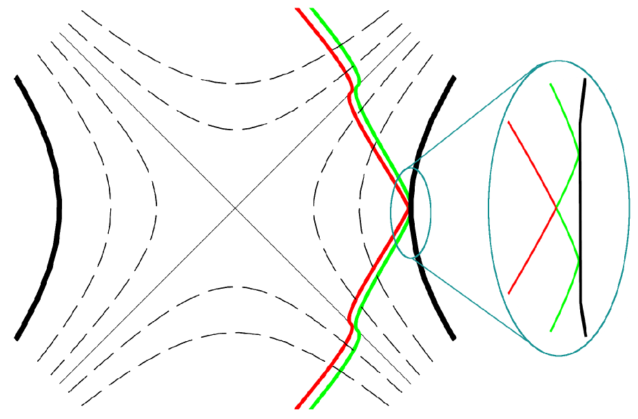
Figure 1: A Kruskal plot of the entire solution, in the spirit of Chen et al. [11]. The exact trajectories of the positive- and negative-tension branes are plotted in red and green respectively, while the naked singularity is indicated by a thick black line. Representative orbits of the bulk Killing vector field are shown with dashed lines, while the solid straight lines indicate the Boyer axes. The bounces of the negative-tension brane off the naked singularity, as well as the collision of the branes themselves, are shown at a magnified scale in the inset. In this plot, we have chosen the relative rapidity of the brane collision to be $2y_{0}=1$. Analogous plots for greater collision rapidities may be found in Figure 4 of Appendix C.

The outline of this paper is as follows. In Section 2, we review the standard static solution of heterotic M-theory and fix notation. In Section 3, we derive the colliding brane solution in brane-comoving coordinates, as an expansion in the rapidity of the brane collision. In Section 4, we discuss the same solution in a coordinate system in which the bulk is static and the branes are moving. Considering the relevant modified Friedmann equation, we then show how the negative-tension brane bounces when an arbitrarily small amount of matter is present on the brane. Three appendices are devoted to technical matters. The first proves a Birkhoff-like theorem for the bulk. The second derives the equations governing the motion of branes in the bulk, and the third discusses the Kruskal extension of the bulk geometry. These calculations are used to make accurate plots of the brane trajectories, like that shown in Figure 1.

2 Heterotic M-theory

Eleven-dimensional supergravity can be compactified on a Calabi-Yau 3-fold to give a minimal five-dimensional supergravity theory [1, 2, 6, 7]. Although the dimensional reduction of the graviton and the 4-form flux generates a large number of fields, it is consistent to retain only the five-dimensional graviton, and a scalar $\phi$ parameterising the volume of the Calabi-Yau manifold (namely $V_{\mathrm{CY}}=e^{\phi}$). This theory can be consistently coupled to two four-dimensional boundary brane actions, provided that one keeps, in addition to gravity and the scalar, the components of the 4-form flux with all indices pointing in the Calabi-Yau directions. This flux thus appears as a scalar in five dimensions (albeit a constant one, as can be seen from its Bianchi identity [6, 7]), and it leads to a potential for $\phi.$ The resulting dimensionally reduced effective action is given by

$$S = \int_{5d}\sqrt{-g}\,[R-\frac{1}{2}(\partial\phi)^{2}-6\alpha^{2}e^{-2\phi}]$$ (2.1)

$$+12\alpha\int_{4d,\,y=-y_{0}}\sqrt{-g^{-}}\,e^{-\phi}-12\alpha\int_{4d,\,y=+y_{0}}\sqrt{-g^{+}}\,e^{-\phi},$$

where $\alpha$ is related to the number of units of 4-form flux, and where we have placed branes of opposite tensions at $y=\pm y_{0}$ ($y$ being the coordinate transverse to the branes). In brane-comoving coordinates, the resulting equations of motion are

$$G_{ab} = \frac{1}{2}\phi_{,a}\phi_{,b}-\frac{1}{4}g_{ab}\phi^{,c}\phi_{,c}-3g_{ab}\,\alpha^{2}e^{-2\phi}$$ (2.2)

$$+6\alpha[\delta(y+y_{0})-\delta(y-y_{0})]\delta_{a}^{\mu}\delta_{b}^{\nu}g_{\mu\nu}\frac{1}{\sqrt{g_{yy}}}\,e^{-\phi},$$

$$\Box\phi = -12\alpha^{2}e^{-2\phi}+12\alpha[\delta(y+y_{0})-\delta(y-y_{0})]\frac{1}{\sqrt{g_{yy}}}\,e^{-\phi},$$ (2.3)

where Latin indices run over all five dimensions, but Greek indices run over only the four dimensions to which the $y$ coordinate is normal. The static domain wall vacuum solution is given by

$$\mathrm{d}s^{2} = h^{2/5}(y)(\eta_{\mu\nu}\mathrm{d}x^{\mu}\mathrm{d}x^{\nu}+\mathrm{d}y^{2}),$$

$$e^{\phi} = h^{6/5}(y),$$

$$h(y) = 5\alpha(y+y_{0})+c,\qquad-y_{0}\leq y\leq y_{0}.$$ (2.4)

The $y$ coordinate is taken to span the orbifold $S^{1}/\mathbb{Z}_{2}$, with fixed points at $\pm y_{0}$. In an ‘extended’ picture of the solution, obtained by $\mathbb{Z}_{2}$-reflecting the solution across the branes, there is a downward-pointing kink at $y=-y_{0}$ and an upward-pointing kink at $y=+y_{0}$. These ensure that the appropriate Israel matching conditions are satisfied, with the negative-tension brane being located at $y=-y_{0}$ and the positive-tension brane at $y=+y_{0}$. The integration constant $c$ is arbitrary.

3 A cosmological solution with colliding branes

We now wish to generalise the static solution above to allow for time dependence. In particular, we are interested in cosmological solutions in which the two boundary branes collide, with the five-dimensional spacetime geometry about the collision reducing to (2d compactified Milne)$/\mathbb{Z}_{2}\times\mathbb{R}^{3}$. We will therefore take as our metric ansatz

$$\mathrm{d}s^{2}=n^{2}(t,y)(-\mathrm{d}t^{2}+t^{2}\mathrm{d}y^{2})+b^{2}(t,y)\,\mathrm{d}\vec{x}\,^{2},$$ (3.1)

where the $x^{i}$ span the three-dimensional spatial worldvolume of the branes, which we are assuming to be flat. This ansatz is in fact the most general form consistent with three-dimensional spatial homogeneity and isotropy, after we have made use of our freedom to write the ($t$, $y$) part of the metric in conformally flat Milne form. In the above, and throughout this section, we will take the branes to be fixed at the constant coordinate locations $y=\pm y_{0}$.

The functions $n$ and $b$, as well as the scalar field $\phi$, are arbitrary functions of $t$ and $y$. In order that the collision be the ‘least singular’ possible, we require that the brane scale factors, as well as the Calabi-Yau volume, be finite and non-zero at the collision. By an appropriate choice of units, we will therefore demand that $n$, $b$ and $e^{\phi}$ all tend to unity as $t\rightarrow 0$. In this way the geometry about the collision reduces to the desired (2d compactified Milne)$/\mathbb{Z}_{2}\times\mathbb{R}^{3}$ times a finite-volume Calabi-Yau manifold. Since the five-dimensional part of this geometry is flat, our solution will be protected from higher-derivative string or M-theory corrections in the vicinity of the collision.

To solve the relevant equations of motion, (2.2) and (2.3), we will perform a perturbative expansion in the rapidity of the brane collision. This latter quantity is given by $2y_{0}$ (see e.g. [14]), and so we are interested in the case in which $y_{0}\ll 1$, i.e., the case in which the relative velocity of the branes at the collision is small. (See [12] for an analogous procedure in the case of the Randall-Sundrum model).

To implement this expansion, we first introduce the re-scaled time and orbifold coordinates

$$\omega=y/y_{0},\qquad T=y_{0}t,$$ (3.2)

so that the branes are now located at $\omega=\pm 1$, independent of the rapidity of the brane collision. For convenience, we will also adopt the convention that primes denote derivatives with respect to $\omega$ and dots denote derivatives with respect to $\ln{T}$, i.e.,

$${}^{\prime}\equiv\partial_{\omega},\qquad\dot{\,}\equiv T\partial_{T}.$$ (3.3)

In order to write down the junction conditions and the Einstein equations, it is useful to work with the variables $e^{\beta}=b^{3}$ and $e^{\nu}=y_{0}nt=nT$. The junction conditions [15], valid when evaluated at $\omega=-1^{+}$ or $\omega=+1^{-}$, are then

$$\nu^{\prime}=\alpha\,e^{\nu-\phi},\qquad\beta^{\prime}=3\alpha\,e^{\nu-\phi},\qquad\phi^{\prime}=6\alpha\,e^{\nu-\phi}.$$ (3.4)

Evaluating the $\phi$, $G^{0}_{0}+G^{5}_{5}$, $G^{5}_{5}$, $G^{0}_{0}+G^{5}_{5}-(1/2)G^{i}_{i}$, and $G_{05}$ equations in the bulk, we obtain the following set of equations:

$$\phi^{\prime\prime}+\beta^{\prime}\phi^{\prime}+12\alpha^{2}e^{2\nu-2\phi} = y_{0}^{2}\,(\ddot{\phi}+\dot{\beta}\dot{\phi}),$$ (3.5)

$$\beta^{\prime\prime}+\beta^{\prime 2}+6\alpha^{2}e^{2\nu-2\phi} = y_{0}^{2}\,(\ddot{\beta}+\dot{\beta}^{2}),$$ (3.6)

$$\frac{1}{3}\,\beta^{\prime 2}+\beta^{\prime}\nu^{\prime}-\frac{1}{4}\,\phi^{\prime 2}+3\alpha^{2}e^{2\nu-2\phi} = y_{0}^{2}\,(\ddot{\beta}+\frac{2}{3}\dot{\beta}^{2}-\dot{\beta}\dot{\nu}+\frac{1}{4}\,\dot{\phi}^{2}),$$ (3.7)

$$\nu^{\prime\prime}-\frac{1}{3}\,\beta^{\prime 2}+\frac{1}{4}\,\phi^{\prime 2}-\alpha^{2}e^{2\nu-2\phi} = y_{0}^{2}\,(\ddot{\nu}-\frac{1}{3}\,\dot{\beta}^{2}+\frac{1}{4}\,\dot{\phi}^{2}),$$ (3.8)

$$\dot{\beta}^{\prime}+\frac{1}{3}\,\dot{\beta}\beta^{\prime}-\dot{\nu}\beta^{\prime}-\nu^{\prime}\dot{\beta}+\frac{1}{2}\,\dot{\phi}\phi^{\prime} = 0.$$ (3.9)

In the above, both the $G^{5}_{5}$ equation (3.7) and the $G_{05}$ equation (3.9) involve only single derivatives with respect to $\omega$. Applying the junction conditions, we find that both left-hand sides vanish when evaluated on the branes. The $G_{05}$ equation is then trivially satisfied, while the $G^{5}_{5}$ equation yields the relation

$$\frac{b_{,TT}}{b}+\frac{b_{,T}^{2}}{b^{2}}-\frac{b_{,T}\,n_{,T}}{bn}+\frac{1}{12}\,\phi_{,T}^{2}=0,$$ (3.10)

valid on both branes. Introducing the brane conformal time $\tau$, defined on either brane via $b\,y_{0}\,\mathrm{d}\tau=n\,\mathrm{d}T$, this relation can be re-expressed as

$$\frac{b_{,\tau\tau}}{b}+\frac{1}{12}\,\phi_{,\tau}^{2}=0.$$ (3.11)

Notice that in the Einstein equations (3.5)-(3.8), all terms involving time derivatives appear at $O(y_{0}^{2})$ higher than the terms involving derivatives along the orbifold direction. Thus, solving the equations of motion perturbatively in powers of $y_{0}^{2}$, at zeroth order we have a set of ordinary differential equations in $\omega$. Integrating these differential equations, we obtain the $\omega$ dependence of the solution at leading order, along with three arbitrary functions of time. How these functions are determined will be explained below in Section 3.2. Then, at next-to-leading order, we have a set of ordinary differential equations for the $\omega$ dependence of the solution at $O(y_{0}^{2})$, involving source terms constructed from the time dependence at leading order. Thus, solving the Einstein equations is reduced to an iterative procedure involving the solution of a finite number of ordinary differential equations at each new order in $y_{0}^{2}$.

3.1 Initial conditions

In order to fix the initial conditions for our expansion in $y_{0}^{2}$, it is useful to solve for the bulk geometry about the collision as a series expansion in $t$ (in this section we revert briefly to our original $t$ and $y$ coordinates). Up to terms of order $t^{3}$, the solution corresponding to the Kaluza-Klein zero mode is:

$$n = 1+\alpha\,(\mathrm{sech}{y_{0}}\sinh{y})\,t+\frac{\alpha^{2}}{8}\,\mathrm{sech}^{2}y_{0}\,(9-\cosh{2y_{0}}-8\cosh{2y})\,t^{2},\qquad$$ (3.12)

$$b = 1+\alpha\,(\mathrm{sech}{y_{0}}\sinh{y})\,t+\frac{\alpha^{2}}{4}\,\mathrm{sech}^{2}y_{0}(3+\cosh{2y_{0}}-4\cosh{2y})\,t^{2},\qquad$$ (3.13)

$$e^{\phi} = 1+6\alpha\,(\mathrm{sech}{y_{0}}\sinh{y})\,t-\frac{3\alpha^{2}}{2}\,\mathrm{sech}^{2}y_{0}(2-\cosh{2y_{0}}-\cosh{2y})\,t^{2},\qquad$$ (3.14)

where we have used the junction conditions to fix the arbitrary constants arising in the integration of the bulk equations with respect to $y$. The brane conformal times $\tau_{\pm}$ (where the subscript $\pm$ refers to the brane locations $\omega=\pm 1$, or equivalently, to their tensions) are then given by

$$\tau_{\pm}=\int\frac{n_{\pm}}{b_{\pm}}\,\mathrm{d}t=t+O(t^{3}),$$ (3.15)

in terms of which the brane scale factors $b_{\pm}$ are

$$b_{\pm}=1\pm\alpha\,\tau_{\pm}\tanh{y_{0}}-\frac{3}{2}\,\alpha^{2}\tau_{\pm}^{2}\tanh^{2}{y_{0}}+O(\tau_{\pm})^{3}.$$ (3.16)

3.2 A conserved quantity

As explained above, every time we integrate the bulk Einstein equations at a given order in $y_{0}^{2}$ with respect to $\omega$ we pick up three arbitrary functions of time. Two of these three functions may be determined with the help of the $G^{5}_{5}$ equation evaluated on both branes, namely (3.11). To fix the third arbitrary function, however, a further equation is needed, which we derive below.

Introducing the variable $\chi=\phi-2\beta$, upon subtracting twice (3.6) from (3.5) we find

$$(\chi^{\prime}e^{\beta})^{\prime}=y_{0}^{2}(\dot{\chi}e^{\beta})\dot{\,},$$ (3.17)

which is the massless wave equation $\raise-1.13809pt\hbox{$\Box$}\chi=0$ in this background. Since the junction conditions imply $\chi^{\prime}=0$ on the branes, the left-hand side vanishes upon integrating over $\omega$. A second integration over $\ln T$ then yields

$$\int_{-1}^{+1}\mathrm{d}\omega\,\dot{\chi}e^{\beta}=\gamma,$$ (3.18)

for some constant $\gamma$, which we can set to zero since our initial conditions are such that $\dot{\chi}e^{\beta}\rightarrow 0$ as $T\rightarrow 0$.

Let us now consider solving (3.17) for $\chi$, as a perturbation expansion in $y_{0}^{2}$. Setting $\chi=\chi_{0}+y_{0}^{2}\,\chi_{1}+O(y_{0}^{4})$, and similarly for $\beta$, at zeroth order we have $(\chi_{0}^{\prime}e^{\beta_{0}})^{\prime}=0$. Integrating with respect to $\omega$ introduces an arbitrary function of $T$ which we can immediately set to zero using the boundary condition on the branes, which, when evaluated to this order, read $\chi_{0}^{\prime}=0$. This tells us that $\chi_{0}^{\prime}=0$ throughout the bulk; $\chi_{0}$ is then a function of $T$ only, and can be taken outside the integral in (3.18). Since $\gamma=0$, yet the integral of $e^{\beta}$ across the bulk cannot vanish, it follows that $\chi_{0}$ must be a constant.

At order $y_{0}^{2}$, the right-hand side of (3.17) evaluates to $y_{0}^{2}(\dot{\chi}_{0}e^{\beta_{0}})\dot{\,}$, which vanishes. Evaluating the left-hand side, we have $(\chi_{1}^{\prime}e^{\beta_{0}})^{\prime}=0$, and hence, by a sequence of steps analogous to those above, we find that $\chi_{1}$ must also be constant. It is easy to see that this behavior continues to all orders in $y_{0}^{2}$. We therefore deduce that $\chi=\phi-2\beta$ is exactly constant. Since both $\phi$ and $\beta$ tend to zero as $T\rightarrow 0$, this constant must be zero, and so we find

$$\phi=2\beta.$$ (3.19)

The essence of this result is that a perturbative solution in powers of $y_{0}^{2}$ exists only when $\chi$ is in the Kaluza-Klein zero mode. This may be seen from (3.17), which reduces, in the limit where $T\rightarrow 0$ and $\beta\rightarrow 0$, to $\chi^{\prime\prime}=y_{0}^{2}\ddot{\chi}$. The existence of a perturbative expansion in $y_{0}^{2}$ requires the right-hand side of this equation to vanish at leading order. This is only the case, however, for the Kaluza-Klein zero mode: all the higher modes have a rapid oscillatory time dependence such that the right-hand side does contribute at leading order. For these higher Kaluza-Klein modes, therefore, a gradient expansion does not exist.

Setting $\phi=2\beta$ from now on, returning to (3.11) and recalling that $\beta=3\ln b$, we immediately obtain the equivalent of the Friedmann equation on the branes, namely

$$\Big{(}\frac{b_{,\tau}}{b}\Big{)}_{,\tau}+4\,\Big{(}\frac{b_{,\tau}}{b}\Big{)}^{2}=0.$$ (3.20)

Integrating, the brane scale factors are given by

$$b_{\pm}=\bar{A}_{\pm}(\tau_{\pm}-c_{\pm})^{1/4}.$$ (3.21)

To fix the arbitrary constants $\bar{A}_{\pm}$ and $c_{\pm}$, we need only to expand the above in powers of $\tau_{\pm}$ and compare with (3.16). We find

$$b_{\pm}=\big{[}1\pm(4\alpha\tanh{y_{0}})\,\tau_{\pm}\big{]}^{1/4}.$$ (3.22)

This equation determines the brane scale factors to all orders in $y_{0}^{2}$ in terms of the conformal time on each brane. (As a straightforward check, it is easy to confirm that the $O(\tau_{\pm}^{2})$ terms in (3.16) are correctly reproduced).

3.3 The scaling solution

We are now in a position to solve the bulk equations of motion perturbatively in $y_{0}^{2}$. Setting

$$\beta=\beta_{0}+y_{0}^{2}\,\beta_{1}+O(y_{0}^{4}),\qquad\nu=\nu_{0}+y_{0}^{2}\,\nu_{1}+O(y_{0}^{4}),$$ (3.23)

the leading terms of this expansion (namely $\beta_{0}$ and $\nu_{0}$) constitute a scaling solution, whose form is independent of $y_{0}$ for all $y_{0}\ll 1$. To determine the $\omega$ dependence of this scaling solution, we must solve the bulk equations of motion at zeroth order in $y_{0}^{2}$. Evaluating the linear combination $(\ref{MG00p55})-3[(\ref{MG55})+(\ref{MG0055ii})]$, noting that at this order the right-hand sides all vanish automatically, we find

$$((\beta^{\prime}_{0}-3\nu^{\prime}_{0})e^{\beta_{0}})^{\prime}=0.$$ (3.24)

Using the boundary condition $\beta^{\prime}_{0}-3\nu^{\prime}_{0}=0$ on the branes, we then obtain $\beta_{0}=3\nu_{0}+f(T)$, for some arbitrary function $f(T)$. Substituting back into (3.7) and taking the square root then yields

$$\nu^{\prime}_{0}=\alpha\,e^{-5\nu_{0}-2f},$$ (3.25)

where consistency with the junction conditions (3.4) forced us to take the positive root. Integrating a second time, and re-writing $e^{f}=B^{-15}$, we find

$$e^{\nu_{0}}=B^{6}(T)\,h^{1/5},\qquad e^{\beta_{0}}=B^{3}(T)\,h^{3/5},$$ (3.26)

where $h=5\alpha\omega+C(T)$, with $C(T)$ arbitrary.

In the special case where $B$ and $C$ are both constant, we recover the exact static domain wall solution (2), up to a trivial coordinate transformation. In general, however, these two moduli will be time-dependent. Inverting the relation $b_{\pm}^{5}=B^{5}(\pm 5\alpha+C)$ to re-express $B$ and $C$ in terms of the brane scale factors $b_{\pm}(T)$, we find

$$B^{5}=\frac{1}{10\alpha}\,(b_{+}^{5}-b_{-}^{5}),\qquad C=5\alpha\left(\frac{b_{+}^{5}+b_{-}^{5}}{b_{+}^{5}-b_{-}^{5}}\right).$$ (3.27)

Furthermore, at zeroth order in $y_{0}^{2}$, the conformal times on both branes are equal, since

$$y_{0}\,\mathrm{d}\tau=\frac{n}{b}\,\mathrm{d}T=e^{\nu_{0}-\beta_{0}/3}\,\frac{\mathrm{d}T}{T}=B^{5}(T)\,\frac{\mathrm{d}T}{T}$$ (3.28)

is independent of $\omega$. To this order then, (3.22) reduces to

$$b_{\pm}=(1\pm 4\alpha y_{0}\tau)^{1/4},$$ (3.29)

allowing us to express the moduli in terms of $\tau$ as

$$B^{5}(\tau) = \frac{1}{10\alpha}\,[(1+4\alpha y_{0}\tau)^{5/4}-(1-4\alpha y_{0}\tau)^{5/4}],$$ (3.30)

$$C(\tau) = 5\alpha\left[\frac{(1+4\alpha y_{0}\tau)^{5/4}+(1-4\alpha y_{0}\tau)^{5/4}}{(1+4\alpha y_{0}\tau)^{5/4}-(1-4\alpha y_{0}\tau)^{5/4}}\right].$$ (3.31)

The brane conformal time $\tau$ and the Milne time $T$ are then related by

$$\ln T=10\alpha y_{0}\int[(1+4\alpha y_{0}\tau)^{5/4}-(1-4\alpha y_{0}\tau)^{5/4}]^{-1}\mathrm{d}\tau.$$ (3.32)

Rather than attempting to evaluate this integral analytically, we will simply adopt $\tau$ as our time coordinate in place of $T$. The complete scaling solution is then given by

$$\mathrm{d}s^{2} = h^{2/5}(\tau,\omega)\,\Big{[}B^{2}(\tau)(-\mathrm{d}\tau^{2}+\mathrm{d}\vec{x}\,^{2})+B^{12}(\tau)\mathrm{d}\omega^{2}\Big{]},$$

$$e^{\phi} = B^{6}(\tau)\,h^{6/5}(\tau,\omega),$$

$$h(\tau,\omega) = 5\alpha\omega+C(\tau),$$ (3.33)

with $B(\tau)$ and $C(\tau)$ given in (3.30) and (3.31). This scaling solution solves the bulk Einstein equations and the junction conditions to leading order in our expansion in $y_{0}^{2}$. The subleading corrections at $y_{0}^{2}$ higher order may be obtained in an analogous fashion, although we will not pursue them here.

The expressions above for the scaling solution can also be used to calculate the slope of the ‘warp factor’ appearing in the metric (3.3), namely $hB^{5}$. The slope, which from the Israel matching condition represents the effective strength of the two brane tensions, is given by

$$(hB^{5})^{\prime}=\frac{1}{2}\,\big{[}(1+4\alpha y_{0}\tau)^{5/4}-(1-4\alpha y_{0}\tau)^{5/4}\big{]}.$$ (3.34)

Thus we can picture the brane tensions to be evolving in time. In particular, note that what was a downward-pointing kink before the collision turns into an upward-pointing kink after the collision (and vice versa), while at the collision itself the slope is zero. Thus the tension of the branes swaps over at the collision, with both branes becoming effectively tensionless at the collision itself. (This is another indication that the collision represents a rather mild singularity).

The scaling solution is valid for times in the range $-(4\alpha y_{0})^{-1}<\tau<(4\alpha y_{0})^{-1}$. At $\tau=\pm(4\alpha y_{0})^{-1}$, however, the scale factor on the negative-tension brane vanishes from (3.29) (recalling that the tension of the branes is reversed for $\tau<0$). Since the physical interpretation of these events is much clearer in the alternative coordinate system in which the bulk is static and the branes are moving, we will postpone a full discussion until Section 4.1. (In fact, it will turn out that to continue the solution to times $\tau>(4\alpha y_{0})^{-1}$, we simply need to introduce absolute value signs around all factors of $(1-4\alpha y_{0}\tau)$).

A further quantity of interest, the distance between the branes, evolves as

$$d=\int_{-1}^{+1}h^{1/5}B^{6}=\frac{1}{6\alpha}\,[(1+4\alpha y_{0}\tau)^{3/2}-(1-4\alpha y_{0}\tau)^{3/2}].$$ (3.35)

Thus, for small $\tau$ we have $d\simeq 2y_{0}\tau$, independent of $\alpha$, and for large $\tau$ (imposing an absolute value on the second term), we have $d\simeq(y_{0}\tau/\alpha)^{1/2}$.

3.4 Lifting to eleven dimensions

It is straightforward to lift the scaling solution to eleven dimensions, where the five-dimensional metric and scalar field are both part of the eleven-dimensional metric. The 4-form field strength has a non-zero component in the Calabi-Yau directions only:

$$G_{abcd}=\frac{\alpha}{\sqrt{2}}\,{\epsilon_{abcd}}^{ef}\,\omega_{ef},\qquad y_{0}<y<y_{0},$$ (3.36)

where $\omega_{ef}$ is the Kähler form on the Calabi-Yau. In the extended picture, the sign of $G_{abcd}$ reverses across the branes. The metric in eleven dimensions reads

$$\mathrm{d}s_{11}^{2} = e^{-2\phi/3}\mathrm{d}s_{5}^{2}+e^{\phi/3}\mathrm{d}s_{\mathrm{CY}}^{2}$$ (3.37)

$$= h^{-2/5}B^{-2}\,(-\mathrm{d}\tau^{2}+\mathrm{d}\vec{x}\,^{2})+h^{-2/5}B^{8}\mathrm{d}\omega^{2}+h^{2/5}B^{2}\mathrm{d}s_{\mathrm{CY}}^{2},$$

and the 4-form flux is proportional to $\alpha$ when all its indices are pointing in a Calabi-Yau direction. Thus the eleven-dimensional distance between the branes is given, to leading order in $y_{0}^{2}$, by

$$d_{11}=B^{4}\int_{-1}^{+1}\mathrm{d}\omega\,h^{-1/5}=2y_{0}\tau.$$ (3.38)

This simple relationship underlies the utility of $\tau$ as a time coordinate.

Finally, the volume of the Calabi-Yau manifold, averaged over the orbifold, is

$$\langle e^{\phi}\rangle=\frac{1}{2}B^{6}\int_{-1}^{+1}\mathrm{d}\omega\,h^{6/5}=\frac{5}{11}\left[\frac{(1+4\alpha y_{0}\tau)^{11/4}-|1-4\alpha y_{0}\tau|^{11/4}}{(1+4\alpha y_{0}\tau)^{5/4}-|1-4\alpha y_{0}\tau|^{5/4}}\right],$$ (3.39)

where we have imposed the absolute values to permit a continuation to late times, as will be explained in Section 4.1. Thus the radius of the Calabi-Yau grows at large times as $\langle e^{\phi/6}\rangle\sim\tau^{1/4}$, whereas the distance between the branes $d_{11}$ grows linearly in $\tau$. A phenomenologically acceptable configuration where $d_{11}\simeq 30\,e^{\phi/6}$ [16] is therefore quite naturally obtained, assuming that both the distance between the branes and the Calabi-Yau volume modulus are stabilised by an inter-brane potential when they reach large values. We will leave a more detailed investigation of the eleven-dimensional properties of our solution to future work.

4 An alternative perspective: moving branes in
a static bulk

Let us now consider an alternative coordinate system in which the bulk is static and the branes are moving. To find the bulk metric in this coordinate system we can make use of a modified version of Birkhoff’s theorem, as shown in Appendix A. Assuming only three-dimensional homogeneity and isotropy, as consistent with cosmological symmetry on the branes, in addition to the exact relation $\phi=2\beta$ (motivated in Section 3.2 through considerations of regularity at the brane collision), the bulk Einstein equations can be integrated exactly. One can then choose the static parameterisation:

$$\mathrm{d}s^{2} = -f\,\mathrm{d}t^{2}+\frac{r^{12}}{f}\,dr^{2}+r^{2}\,\mathrm{d}\vec{x}^{2},$$

$$f(r) = \alpha^{2}r^{2}-\mu r^{4},\qquad e^{\phi}=r^{6},$$ (4.1)

where $0\leq r\leq\sqrt{\mu}/\alpha$, and the coordinate $t$ is unrelated to the Milne time appearing in the previous section. Physically, this solution describes a timelike naked singularity located at $r=0$, and was first discovered by Chamblin and Reall in [10] (who instead looked directly for solutions in which the bulk was static). Since the coordinates above do not cover the whole spacetime manifold, the maximal extension may easily be constructed following the usual Kruskal procedure, as detailed in Appendix C.

To find the trajectories of a pair of positive- and negative-tension branes embedded in this static bulk spacetime we solve the Israel matching conditions in the usual fashion. After performing this calculation (see Appendix B, and also [10]), one finds that the induced brane metrics are indeed cosmological, with scale factors given by

$$b_{\pm}=(1\pm 4\sqrt{\mu}\,\tau_{\pm})^{1/4},$$ (4.2)

where $\tau_{\pm}$ is the brane conformal time, and we have rescaled $b_{\pm}$ to unity at the collision, which is taken to occur at $\tau_{\pm}=0$.

Upon setting $\mu=0$, we immediately recover the static domain wall solution (2), after a suitable change of coordinates. More generally, we require $\mu\geq 0$ to avoid the appearance of imaginary scale factors. Through comparison with our earlier result (3.22), we also find

$$\sqrt{\mu}=\alpha\,\tanh{y_{0}}.$$ (4.3)

Thus, for $\mu>0$, after starting off coincident, the two branes proceed to separate. However, while the positive-tension brane travels out to large radii unchecked, the negative-tension brane reaches the naked singularity (at which $b_{-}$ and $e^{\phi}$ tend to zero) in a finite brane conformal time $\tau_{-}=(4\sqrt{\mu})^{-1}$.

In the following section we will argue that the resulting singularity is extremely mild, and simple to regularise. If almost any type of well-behaved matter is present on the negative-tension brane – even in only vanishing quantities – then, rather than hitting the singularity, the negative-tension brane will instead undergo a bounce at some small finite value of the scale factor and move away from the singularity.

4.1 The bounce of the negative-tension brane

The Friedmann equation for the negative-tension brane is derived in Appendix B. For the case in which a time-dependent scalar field (with an $e^{\phi}$ coupling to the Calabi-Yau volume scalar) is present on the brane, this equation takes the form (see (B.13))

$$H_{-}^{2}=\frac{\dot{b}_{-}^{2}}{b_{-}^{2}}=-2\alpha\,\frac{A_{-}}{b_{-}^{18}}+\frac{A_{-}^{2}}{b_{-}^{24}}+\frac{\mu}{b_{-}^{10}},$$ (4.4)

where the constant $A_{-}$ parameterises the scalar kinetic energy density.

The key feature of this equation is the negative sign in front of the first term on the right-hand side, reflecting the fact that matter on the negative-tension brane couples to gravity with the wrong sign. For sufficiently large values of the scale factor the right-hand side is dominated by the $\mu\,b_{-}^{-10}$ term. If we further assume that the matter density on the branes is small compared to the brane tension (i.e. $A_{-}\ll\alpha$), so that the term linear in $A_{-}$ dominates over the quadratic term, then it follows that at some small value of the scale factor the entire right-hand side must vanish. Thus a negative-tension brane, initially travelling towards the singularity, will generically undergo a smooth bounce at some small value of the scale factor. After this bounce the brane travels away from the singularity back towards large values of the scale factor. This behaviour is specific to the negative-tension brane, and moreover, persists even in the limit in which $A_{-}$ (and hence the initial matter density) is negligibly small.

In fact, even in the complete absence of matter on the negative-tension brane, the bounce off the naked singularity is still a relatively smooth event: converting to Kruskal coordinates so that light rays are at $\pm\pi/4$ angles, using our exact solution we show in Appendix C that the trajectory of the negative-tension brane becomes precisely tangential to the singularity at the moment of the bounce. In these coordinates then, the negative-tension brane merely grazes the singularity with zero velocity, before moving away again according to a well-defined smooth continuation. The complete solution is illustrated in Figures 1 and 4.

In this solution, the scale factor on the negative-tension brane is given exactly for all times post-collision by

$$b_{-}=|1-4\sqrt{\mu}\,\tau_{-}|^{1/4},$$ (4.5)

where $\tau_{-}$ is the conformal time on the negative-tension brane. This result shows us how to continue our earlier scaling solution in brane-comoving coordinates (see Section 3.3) to times after the bounce of the negative-tension brane: we simply insert an absolute value sign into the expression (3.29) for $b_{-}$ (recalling that $\tau$ is indeed the brane conformal time in these coordinates). The moduli $B(\tau)$ and $C(\tau)$ then follow from (3.27), which amounts to replacing all factors of $(1-4\alpha y_{0}\tau)$ in (3.30) and (3.31) with $|1-4\alpha y_{0}\tau|$. It is easy to check that this continuation does not affect the smooth evolution of quantities defined on the positive-tension brane, and that the range of the coordinate $\omega$ along the extra dimension is unaltered by this continuation (see Figure 2). Nevertheless, this brane-comoving coordinate system is not particularly well-adapted to deal with the actual moment of the bounce itself, as evidenced by the ‘kinks’ in Figure 2. With the presence of regulatory matter on the negative-tension brane, however, the bounce will occur at some small non-zero $b_{-}$, smoothing out these kinks.

\psfrag{b4}{$b^{4}$}\psfrag{t}{$\alpha y_{0}\tau$}\includegraphics[width=341.43306pt]{newHWplot.eps}

Figure 2: Continuation of the scaling solution (accurate to leading order in $y_{0}$) beyond the bounce of the negative-tension brane at $\alpha y_{0}\tau=1/4$, using the absolute value prescription. Contours of constant $\omega$ are plotted against the fourth power of the three-dimensional scale factor $b$ and the brane conformal time $\tau$. The contours shown are, from left to right, $\omega=-1$, $-0.75$, $-0.5$, $0$, $0.5$, and $1$. Thus the left-most and right-most trajectories correspond to the negative- and positive-tension branes respectively (for which $b_{\pm}^{4}=|1\pm 4\alpha y_{0}\tau|$), with the region in between representing the bulk.

To check that the scaling solution is qualitatively correct near the bounce of the negative-tension brane, it is interesting to examine the leading behaviour of the exact bulk metric about the singularity. Setting $r^{5}=5\rho+c$, for some constant $c$, the metric (4) becomes

$$\mathrm{d}s^{2}=(5\rho+c)^{2/5}\left[-\big{(}\alpha^{2}-\mu(5\rho+c)^{2/5}\big{)}\mathrm{d}t^{2}+\mathrm{d}\vec{x}^{2}+\frac{\mathrm{d}\rho^{2}}{\alpha^{2}-\mu(5\rho+c)^{2/5}}\right],$$ (4.6)

which, after trivial re-scalings, to leading order in $r$ reads

$$\mathrm{d}s^{2}=(5\rho+c)^{2/5}[-\mathrm{d}t^{2}+\mathrm{d}\vec{x}^{2}+\mathrm{d}\rho^{2}].$$ (4.7)

This is precisely the form of our scaling solution (3.3) at a given instant in time.

Note also that in the exact solution, the proper velocity of the negative-tension brane vanishes as it approaches the naked singularity: from (4) the proper velocity is $r^{6}\mathrm{d}r/(f\mathrm{d}t)$, which scales as $r^{4}\mathrm{d}r/\mathrm{d}t$ at small $r$. Yet from (C.5), $\mathrm{d}r/\mathrm{d}t$ scales as $f/r^{5}\sim 1/r^{3}$, and so the proper velocity tends to zero linearly with $r$. This result, that the proper velocity of the negative-tension brane tends to zero linearly with $r$ as it approaches the naked singularity, is also found in Kruskal coordinates, as shown in (C.14).

5 Conclusions

We have presented a cosmological solution describing the collision of the two flat boundary branes in heterotic M-theory. This solution is a significant step towards our goal of describing the cosmic singularity as a brane collision within the well-motivated framework of Hořava-Witten theory. Requiring the collision to be the ‘least singular’ possible, i.e., that the metric tends towards (2d compactified Milne)$/\mathbb{Z}_{2}\times\mathbb{R}_{3}$ times a finite-volume Calabi-Yau, has two important consequences. First, it selects a single solution to the equations of motion. Second, it shifts the singularity in the Calabi-Yau volume that one might have naively expected at the brane collision to two spacetime events before and after the brane collision. We have shown these two events to be very mild singularities, which are easily removed by including an arbitrarily small amount of matter (for example scalar field kinetic energy) on the negative-tension brane. Before the initial bounce of the negative-tension brane, and after the final bounce, the solution presented here can be identified with that described by Chen et al. [11].

When the branes move at a small velocity, we expect to be able to accurately describe the solution using a four-dimensional effective theory (see e.g. [18, 19, 21, 22, 20] and also [12]). We shall present such a description in a companion publication [23].

If our colliding brane solution is to successfully describe the universe, we must also add potentials capable of stabilising the moduli; in particular the volume of the Calabi-Yau manifold, which determines the value of gauge couplings, and the distance between the branes, which determines Newton’s constant of gravitation. These potentials also permit us to generate an interesting spectrum of cosmological perturbations. Although the required potentials cannot yet be derived from first principles, we can study the consequences of various simple assumed forms. The results will be presented elsewhere [24].

***

Acknowledgements: The authors wish to thank Mariusz Dabrowski, Gary Gibbons, André Lukas, Ian Moss, Chris Pope, Paul Steinhardt, Kelly Stelle and Andrew Tolley for useful discussions. JLL and NT acknowledge the support of PPARC and of the Centre for Theoretical Cosmology, in Cambridge. PLM is supported through a Spinoza Grant of the Dutch Science Organisation (NWO).

Appendix A A modified Birkhoff theorem

In this appendix we show how the assumption of cosmological symmetry on the branes, coupled with the exact result $\phi=2\beta$ (derived in Section 3.2 following from our assumption that the Riemann curvature remains bounded as we approach the collision), is sufficient to uniquely determine the bulk metric. Moreover, with an appropriate choice of time-slicing, the bulk geometry can be written in static form. Our derivation closely parallels the analogous case for the Randall-Sundrum model [25].

We start with the fully-general metric ansatz

$$\mathrm{d}s^{2}=e^{2\sigma-2\psi/3}(-\mathrm{d}t^{2}+\mathrm{d}y^{2})+e^{2\psi/3}\mathrm{d}\Omega_{3}^{2},$$ (A.1)

where $\sigma(t,y)$ and $\psi(t,y)$ are arbitrary functions, and the coordinates $t$ and $y$ are fresh, unrelated to those appearing earlier. To allow for the possibility of open, flat or closed brane geometries, we will take

$$\mathrm{d}\Omega_{3}^{2}=(1-k\rho^{2})^{-1}\mathrm{d}\rho^{2}+\rho^{2}\mathrm{d}\Omega_{2}^{2},$$ (A.2)

where $k=-1$, $0$ or $+1$ respectively, and $\mathrm{d}\Omega_{2}^{2}$ denotes the usual line element on a unit two-sphere. The above choice represents the most general bulk metric consistent with three-dimensional spatial homogeneity and isotropy, after we have made use of our freedom to write the ($t$, $y$) part of the metric in a conformally flat form.

In light of Section 3.2, we will additionally set $\phi=2\psi$. Then, evaluating the Einstein equations (3.5)-(3.9) in the bulk, after taking appropriate linear combinations we find

$$\psi_{,ty} = \sigma_{,y}\psi_{,t}+\sigma_{,t}\psi_{,y}-3\psi_{,t}\psi_{,y},$$ (A.3)

$$\psi_{,tt}+\psi_{,yy} = 2\sigma_{,t}\psi_{,t}+2\sigma_{,y}\psi_{,y}-3\psi_{,t}^{2}-3\psi_{,y}^{2},$$ (A.4)

$$\psi_{,tt}-\psi_{,yy} = -\psi_{,t}^{2}+\psi_{,y}^{2}+6\alpha^{2}e^{2\sigma-14\psi/3},$$ (A.5)

$$\sigma_{,tt}-\sigma_{,yy} = -\psi_{,t}^{2}+\psi_{,y}^{2}+\alpha^{2}e^{2\sigma-14\psi/3}+2ke^{2\sigma-4\psi/3}.$$ (A.6)

Switching to the light-cone coordinates,

$$u=\frac{1}{2}\,(t-y),\qquad v=\frac{1}{2}\,(t+y),$$ (A.7)

these become

$$\psi_{,uu} = 2\sigma_{,u}\psi_{,u}-3\psi_{,u}^{2},$$ (A.8)

$$\psi_{,vv} = 2\sigma_{,v}\psi_{,v}-3\psi_{,v}^{2},$$ (A.9)

$$\psi_{,uv} = -\psi_{,u}\psi_{,v}+6\alpha^{2}e^{2\sigma-14\psi/3},$$ (A.10)

$$\sigma_{,uv} = -\psi_{,u}\psi_{,v}+\alpha^{2}e^{2\sigma-14\psi/3}+2ke^{2\sigma-4\psi/3}.$$ (A.11)

Integrating the first two equations, we find

$$e^{2\sigma-3\psi}=\psi_{,u}V^{\prime}(v)=\psi_{,v}U^{\prime}(u),$$ (A.12)

where $U^{\prime}(u)$ and $V^{\prime}(v)$ are arbitrary non-zero functions, and we will use primes to denote ordinary differentiation wherever the argument of a function is unique. It follows that $\psi$ and $\sigma$ take the form

$$\psi=\psi(U(u)+V(v)),\qquad e^{2\sigma-3\psi}=\psi^{\prime}U^{\prime}V^{\prime}.$$ (A.13)

Consistency between (A.10) and (A.11) then requires $k=0$, and so only spatially flat three-geometries are permitted. Integrating once, we find

$$\psi^{\prime}e^{\psi}=9\mu-9\alpha^{2}e^{-2\psi/3},$$ (A.14)

where $\mu$ is an arbitrary constant.

The metric

$$\mathrm{d}s^{2}=-4\psi^{\prime}e^{7\psi/3}\mathrm{d}U\mathrm{d}V+e^{2\psi/3}\mathrm{d}\vec{x}^{2},$$ (A.15)

upon changing coordinates to

$$r=e^{\psi/3},\qquad t=3(V-U),$$ (A.16)

then takes the static form

$$\mathrm{d}s^{2}=-(\alpha^{2}r^{2}-\mu r^{4})\,\mathrm{d}t^{2}+\frac{r^{12}\mathrm{d}r^{2}}{(\alpha^{2}r^{2}-\mu r^{4})}+r^{2}\mathrm{d}\vec{x}^{2}.$$ (A.17)

The corresponding Calabi-Yau volume is given by

$$e^{\phi}=r^{6}.$$ (A.18)

Appendix B Brane trajectories

In this appendix we embed a pair of moving branes into the static bulk spacetime (A.17) and derive the Friedmann equations describing their trajectories. This is accomplished by solving the Israel matching conditions [15]:

$$K^{\pm}_{ab}=-\frac{1}{2}\,\big{(}T^{\pm}_{ab}-\frac{1}{3}\,g^{\pm}_{ab}\,T^{\pm}\big{)},$$ (B.1)

where $K^{\pm}_{ab}$, $T^{\pm}_{ab}$ and $g^{\pm}_{ab}$ denote the brane extrinsic curvature, stress tensor and induced metric respectively, and we are assuming a $\mathbb{Z}_{2}$ symmetry about each brane.

Parameterising the trajectory of a given brane as $t=T\,(t_{p})$ and $r=R\,(t_{p})$, where $t_{p}$ is the brane proper time, the induced metric is

$$\mathrm{d}s^{2}=-\mathrm{d}t_{p}^{2}+R^{2}(t_{p})\,\mathrm{d}\vec{x}^{2},$$ (B.2)

hence $R$ may be associated with the relevant brane scale factor $b_{\pm}$. The brane 4-velocity is then $u^{a}=(\dot{T},\,\dot{R},\,\vec{0})$, where, throughout this appendix, we will use dots to indicate differentiation with respect to $t_{p}$. The constraint $u^{a}u_{a}=-1$ yields the additional relation $\dot{T}=(f+R^{12}\dot{R}^{2})^{1/2}/f$. Similarly, the unit normal vector $n^{a}$ is given by

$$n_{a}=\pm(R^{6}\dot{R},\,-\frac{R^{6}}{f}\,(f+R^{12}\dot{R}^{2})^{1/2},\,\vec{0}),$$ (B.3)

where the function $f(r)$ is as defined in (4). (Note that the choice of sign corresponds to our choice of which side of the bulk we keep prior to imposing the $\mathbb{Z}_{2}$ symmetry. Keeping the side for which $r\leq R(t_{p})$ leads to the creation of a positive-tension brane, with normal pointing in the direction of decreasing $r$, requiring the positive sign for $n_{a}$. Conversely, if we retain the $r\geq R(t_{p})$ side of the bulk creating a negative-tension brane, the normal points in the direction of increasing $r$ and we must take the negative sign for $n_{a}$).

The three-spatial components of the brane extrinsic curvature are then

$$K^{\pm}_{ij}=\nabla_{i}n_{j}^{\pm}=\mp R^{-7}(f+R^{12}\dot{R}^{2})^{1/2}\,g^{\pm}_{ij},$$ (B.4)

while the brane stress-energy is given by $T^{\pm}_{ab}=\mp 6\alpha e^{-\phi}g^{\pm}_{ab}$. The Israel matching condition then yields the Friedmann equation $H_{\pm}^{2}=\dot{R}^{2}/R^{2}=\dot{b}_{\pm}^{2}/b_{\pm}^{2}=\mu/b_{\pm}^{10}$. Integrating, we find [10]

$$b_{\pm}=(1\pm 5\sqrt{\mu}\,t_{p}^{\pm})^{1/5},$$ (B.5)

where the constants of integration have been fixed by re-scaling $b_{\pm}$ to unity at the collision, which is taken to occur at $t_{p}^{\pm}=0$. In terms of brane conformal time $\tau_{\pm}$, this relation reads

$$b_{\pm}=(1\pm 4\sqrt{\mu}\,\tau_{\pm})^{1/4},$$ (B.6)

where the origins of $\tau_{\pm}$ are chosen so that the branes collide at $\tau_{\pm}=0$.

This result may easily be generalised to scenarios in which matter is incorporated on one or both of the branes. For example, in the case where we add a scalar field $\chi$ on each brane, allowing for an arbitrary coupling $F(\phi)$ to the Calabi-Yau volume modulus $\phi$, the action should be augmented by the terms

$$-\int_{4d,\,\omega=\pm 1}\sqrt{-g^{\pm}}\,\frac{1}{2}\,(\partial\chi)^{2}\,F(\phi).$$ (B.7)

The brane stress-energy is now

$$T^{\pm}_{ab}=\mp 6\alpha e^{-\phi}g^{\pm}_{ab}+\frac{1}{2}F(\phi)\,[\chi_{,a}\chi_{,b}-\frac{1}{2}\,g^{\pm}_{ab}\,(\partial\chi)^{2}].$$ (B.8)

Since we are interested in cosmological solutions, we will consider the scalar field $\chi$ to be a function of time only. Evaluating the three-spatial components of (B.1) then yields the modified Friedmann equation

$$H_{\pm}^{2}=\pm\frac{\alpha}{12}\,\frac{\dot{\chi}^{2}F}{b_{\pm}^{6}}+\frac{\dot{\chi}^{4}F^{2}}{24^{2}}+\frac{\mu}{b_{\pm}^{10}}.$$ (B.9)

To find the dependence of $\chi$ on the scale factor $b_{\pm}$, it is necessary to evaluate the $t_{p}t_{p}$ component of (B.1). This yields the equivalent of the usual cosmological energy conservation equations. We start with

$$K_{t_{p}t_{p}}=K_{ab}u^{a}u^{b}=u^{a}u^{b}\nabla_{a}n_{b}=-n_{c}a^{c},$$ (B.10)

where the acceleration $a^{c}=u^{b}\nabla_{b}u^{c}$. Since $a^{c}u_{c}=0$, the acceleration may also be written as $a^{c}=an^{c}$, where $a=-K_{t_{p}t_{p}}$. Then, since $\partial_{t}$ is a Killing vector of the background, we have $a=\dot{u}_{t}/n_{t}$. Thus (B.1) reads

$$K^{\pm}_{t_{p}t_{p}}=\pm\frac{1}{R^{6}\dot{R}}\,\frac{\mathrm{d}}{\mathrm{d}t_{p}}\,\big{(}\alpha R\pm\frac{1}{24}\,R^{7}\dot{\chi}^{2}F)=\pm\frac{\alpha}{R^{6}}-\frac{5}{24}\,\dot{\chi}^{2}F,$$ (B.11)

where we have used (B.9). This leads to

$$R\,(\dot{\chi}^{2}F)_{,R}=-12\,\dot{\chi}^{2}F,$$ (B.12)

i.e. we have $\dot{\chi}^{2}F=24\,A_{\pm}\,R^{-12}$, for some constant $A_{\pm}$. Thus the Friedmann equation becomes

$$H_{\pm}^{2}=\pm\frac{2\alpha A_{\pm}}{b_{\pm}^{18}}+\frac{A_{\pm}^{2}}{b_{\pm}^{24}}+\frac{\mu}{b_{\pm}^{10}}.$$ (B.13)

We must also satisfy the junction condition arising from the $\phi$ equation of motion. This is given by

$$2\,n^{a}\partial_{a}\phi_{\pm}=\mp 12\alpha\,e^{-\phi}_{\pm}-\frac{1}{2}\,\dot{\chi}^{2}F_{,\phi},$$ (B.14)

which leads to

$$H_{\pm}^{2}=\pm\frac{\alpha}{12}\,\frac{\dot{\chi}^{2}F_{,\phi}}{b_{\pm}^{6}}+\frac{\dot{\chi}^{4}F_{,\phi}^{2}}{24^{2}}+\frac{\mu}{b_{\pm}^{10}}.$$ (B.15)

Consistency with (B.9) then requires the coupling to be

$$F(\phi)=e^{\phi}.$$ (B.16)

It can be verified that this coupling is also consistent with the equation of motion for $\chi$.

Another form of brane-bound matter that alters the Friedmann equations on the branes, while remaining consistent with the bulk geometry, is a cosmological constant $\Lambda$ with $e^{-\phi}$ coupling to the Calabi-Yau volume scalar. In this case, the modified Friedmann equation is given by

$$H_{\pm}^{2}=\pm\frac{\alpha}{3}\,\frac{\Lambda}{b_{\pm}^{12}}+\frac{1}{36}\,\frac{\Lambda^{2}}{b_{\pm}^{12}}+\frac{\mu}{b_{-}^{10}}.$$ (B.17)

We will use the modified Friedmann equations (which are generally similar in form to (B.13)) in Section 4.1, to understand the bounce of the negative-tension brane in the vicinity of the singularity.

Appendix C Kruskal extension of the bulk geometry

In this appendix we consider the maximal extension of the bulk geometry (4), beyond the range $0\leq r\leq\sqrt{\mu}/\alpha$ for which $f\geq 0$. These calculations will lead us to the Kruskal diagram in Figure 1. Following Chen et al. [11], we start with the Eddington-Finkelstein coordinates $u$ and $v$, defined via

$$\mathrm{d}u=4\alpha^{2}\big{(}\mathrm{d}t+\frac{r^{6}}{f}\,\mathrm{d}r\big{)},\qquad\mathrm{d}v=4\alpha^{2}\big{(}\mathrm{d}t-\frac{r^{6}}{f}\,\mathrm{d}r\big{)}.$$ (C.1)

The entire spacetime manifold is then covered by the Kruskal coordinates

$$U=\exp\left(-\frac{\lambda^{2}}{4}\,u\right),\qquad V=\exp\left(\frac{\lambda^{2}}{4}\,v\right),$$ (C.2)

where, for later convenience, we have introduced the constant $\lambda=\sqrt{\mu}/\alpha=\tanh y_{0}$. In these coordinates, the metric then reads

$$\mathrm{d}s^{2}=\frac{f}{\alpha^{4}\lambda^{4}}\,\frac{\mathrm{d}U\mathrm{d}V}{UV}+r^{2}\mathrm{d}\vec{x}^{2}.$$ (C.3)

Note that $r$ should be understood here as a function of $UV$, given implicitly by

$$UV=\sigma\exp\left[\frac{2}{\lambda^{3}}\,\left(\bar{r}+\frac{1}{3}\,\bar{r}^{3}-\frac{1}{2}\,\ln\left|\frac{1+\bar{r}}{1-\bar{r}}\right|\right)\right],$$ (C.4)

where the re-scaled radial coordinate $\bar{r}=\lambda r$, and $\sigma$ is defined such that $\sigma=+1$ for $0\leq\bar{r}\leq 1$, while $\sigma=-1$ for $\bar{r}>1$. (This choice generates the smooth continuation illustrated in Figure 3).

\psfrag{UV}{$UV$}\psfrag{r}{$\bar{r}$}\includegraphics[width=284.52756pt]{UVr.eps}

Figure 3: $UV$ plotted as a function of $\bar{r}$, according to (C.4) (taking $\lambda=1$). Note in particular the smooth continuation to $\bar{r}>1$ generated by the sign flip in $\sigma$. The surfaces of constant $\bar{r}$ correspond to the hyperbolae $UV=\mathrm{constant}$, with this constant being positive for $0\leq\bar{r}<1$, and negative for $\bar{r}>1$.

Surfaces of constant $\bar{r}$ thus correspond to the hyperbolae $UV=\mathrm{constant}$. In particular, we have chosen the constant of integration deriving from (C.1) such that the singularity at $\bar{r}=0$ maps to the hyperbola $UV=1$. The second constant of integration implicit in (C.1) may then be fixed by requiring that the time slice $t=0$ corresponds to the line $U=V$ for $0\leq\bar{r}\leq 1$, in which case $V/U=\exp(2\lambda^{2}\alpha^{2}t)$.

From the results of the preceding appendix, the trajectory of a brane (in the absence of any additional matter) is given, for $0\leq\bar{r}\leq 1$, by

$$\frac{\mathrm{d}r}{\mathrm{d}t}=\pm\frac{\lambda f}{r^{5}},$$ (C.5)

with the upper and lower signs corresponding respectively to a brane moving away from, and a brane moving towards, the singularity. Specialising to the case of two branes moving in opposite directions, upon integrating we find

$$\mp 2\lambda^{5}\alpha^{2}t=\bar{r}^{2}+\ln(1-\bar{r}^{2})-\lambda^{2}-\ln(1-\lambda^{2}),$$ (C.6)

where we have fixed the constants of integration by requiring that the brane scale factors are unity at the collision (hence $\bar{r}=\lambda$ at $t=0$).

Converting now to Kruskal coordinates, we find the trajectories of the branes are given parametrically, for all $0\leq\bar{r}<\infty$, by

$$U = {\cal F}(\bar{r}),\qquad V=\mathcal{G}(\bar{r})\qquad\mathrm{(outgoing)};$$ (C.7)

$$U = \mathcal{G}(\bar{r}),\qquad V={\cal F}(\bar{r})\qquad\mathrm{(infalling)};$$ (C.8)

where the smooth functions

$${\cal F}(\bar{r}) = \sigma\exp\Big{[}\frac{1}{\lambda^{3}}\,\big{(}\bar{r}+\frac{1}{2}\,\bar{r}^{2}+\frac{1}{3}\,\bar{r}^{3}+\ln|1-\bar{r}|-\frac{1}{2}\,\lambda^{2}-\frac{1}{2}\,\ln(1-\lambda^{2})\big{)}\Big{]},$$ (C.9)

$$\mathcal{G}(\bar{r}) = \ \ \exp\Big{[}\frac{1}{\lambda^{3}}\,\big{(}\bar{r}-\frac{1}{2}\,\bar{r}^{2}+\frac{1}{3}\,\bar{r}^{3}-\ln(1+\bar{r})+\frac{1}{2}\,\lambda^{2}+\frac{1}{2}\,\ln(1-\lambda^{2})\big{)}\Big{]}.$$ (C.10)

As previously, $\sigma=+1$ for $0\leq\bar{r}\leq 1$, but $\sigma=-1$ for $\bar{r}>1$, ensuring that $UV<0$ for the portion of the trajectories parameterised by $\bar{r}>1$.

To extend the brane trajectories beyond the bounce off the naked singularity, we first of all write down the ‘extended’ trajectories in terms of the original $\bar{r}$ and $t$ coordinates. Altering the constants of integration in (C.6) so that the different branches of the trajectories match up at the bounce, we find

$$\mp 2\lambda^{5}\alpha^{2}t=\bar{r}^{2}+\ln(1-\bar{r}^{2})+\lambda^{2}+\ln(1-\lambda^{2}),$$ (C.11)

for $0\leq\bar{r}\leq 1$, where the upper and lower signs correspond respectively to an outgoing, and an infalling, brane. Converting to Kruskal coordinates, this becomes

$$U = {\cal F}(\bar{r})\,\mathcal{G}^{2}(0),\qquad V=\mathcal{G}(\bar{r})\,{\cal F}^{2}(0)\qquad\mathrm{(outgoing)};$$ (C.12)

$$U = \mathcal{G}(\bar{r})\,{\cal F}^{2}(0),\qquad V={\cal F}(\bar{r})\,\mathcal{G}^{2}(0)\qquad\mathrm{(infalling)};$$ (C.13)

where $\bar{r}$ now takes values in the entire range $0\leq r<\infty$. Finally, plotting (C.7), (C.8), (C.12) and (C.13), we obtain the full Kruskal diagrams shown in Figure 1 (for $y_{0}=0.5$), and in Figure 4 (for $y_{0}=1$ and $1.5$).

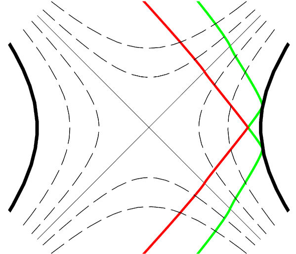
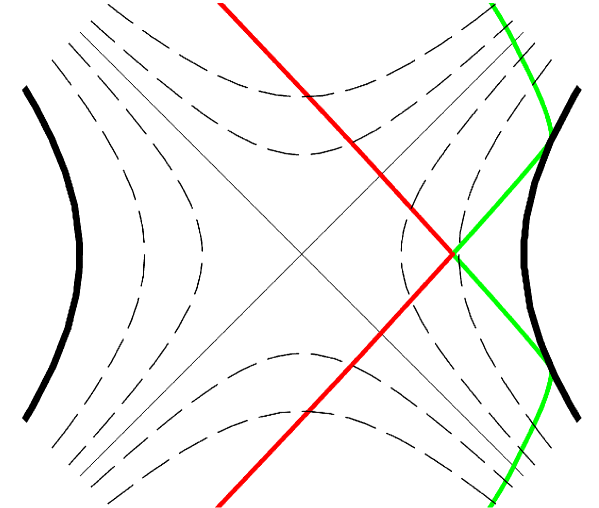
Figure 4: Kruskal diagrams illustrating the brane trajectories for different collision rapidities. In the upper plot $y_{0}=1$, and in the lower plot $y_{0}=1.5$. The corresponding plot for $y_{0}=0.5$ appeared previously in Figure 1.

An interesting feature of the brane trajectories revealed by these plots are the points of inflection that occur whenever the brane trajectories intersect the Boyer axes $UV=0$ (see Figure 1 especially). These may be understood as a consequence of the vanishing of $f$ in (C.5) whenever $\bar{r}=1$.

Note also that at the singularity ($\bar{r}=0$ corresponding to $UV=1$), the slope of the negative-tension brane trajectory is exactly $-1/U^{2}$. For example, using (C.7),

$$\frac{\mathrm{d}V}{\mathrm{d}U}=-\left(\frac{1-\bar{r}}{1+\bar{r}}\right)\frac{V}{U},$$ (C.14)

which reduces to $-1/U^{2}$ when $\bar{r}=0$ and $UV=1$. A similar conclusion applies for each of the other solution branches (C.8), (C.12), (C.13). Consequently, the brane trajectory at the bounce is tangent to the singularity itself. This means that the brane simply grazes the singularity with vanishing normal velocity. Similarly for the Calabi-Yau volume at the branes, $V_{\mathrm{CY}}=r^{6}$, we find

$$\frac{\mathrm{d}V_{\mathrm{CY}}}{\mathrm{d}t}=\pm 6\lambda f=\pm 6\lambda\alpha^{2}r^{2}+O(r^{4}),$$ (C.15)

and hence the rate of change of the Calabi-Yau volume on the negative-tension brane, as it bounces off the singularity, is zero. The above considerations suggest that the bounce of the negative-tension brane is a relatively smooth event, even in the absence of regulatory matter on the brane.

References

- Horava and Witten [1996a] P. Horava and E. Witten, Nucl. Phys. B460, 506 (1996a), hep-th/9510209.
- Horava and Witten [1996b] P. Horava and E. Witten, Nucl. Phys. B475, 94 (1996b), hep-th/9603142.
- Khoury et al. [2001] J. Khoury, B. A. Ovrut, P. J. Steinhardt, and N. Turok, Phys. Rev. D64, 123522 (2001), hep-th/0103239.
- Khoury et al. [2002] J. Khoury, B. A. Ovrut, N. Seiberg, P. J. Steinhardt, and N. Turok, Phys. Rev. D65, 086007 (2002), hep-th/0108187.
- Turok et al. [2004] N. Turok, M. Perry, and P. J. Steinhardt, Phys. Rev. D70, 106004 (2004), hep-th/0408083.
- Lukas et al. [1999a] A. Lukas, B. A. Ovrut, K. S. Stelle, and D. Waldram, Phys. Rev. D59, 086001 (1999a), hep-th/9803235.
- Lukas et al. [1999b] A. Lukas, B. A. Ovrut, K. S. Stelle, and D. Waldram, Nucl. Phys. B552, 246 (1999b), hep-th/9806051.
- Moss [2003] I. G. Moss, Phys. Lett. B577, 71 (2003), hep-th/0308159.
- Moss [2005] I. G. Moss, Nucl. Phys. B729, 179 (2005), hep-th/0403106.
- Chamblin and Reall [1999] H. A. Chamblin and H. S. Reall, Nucl. Phys. B562, 133 (1999), hep-th/9903225.
- Chen et al. [2006] W. Chen, Z. W. Chong, G. W. Gibbons, H. Lu, and C. N. Pope, Nucl. Phys. B732, 118 (2006), hep-th/0502077.
- McFadden et al. [2005] P. L. McFadden, N. Turok, and P. J. Steinhardt (2005), hep-th/0512123.
- Lehners and Stelle [2003] J.-L. Lehners and K. S. Stelle, Nucl. Phys. B661, 273 (2003), hep-th/0210228.
- Tolley et al. [2004] A. J. Tolley, N. Turok, and P. J. Steinhardt, Phys. Rev. D69, 106005 (2004), hep-th/0306109.
- Israel [1966] W. Israel, Nuovo Cim. B44S10, 1 (1966).
- Banks and Dine [1996] T. Banks and M. Dine, Nucl. Phys. B479, 173 (1996), hep-th/9605136.
- Shiromizu et al. [2000] T. Shiromizu, K.-i. Maeda, and M. Sasaki, Phys. Rev. D62, 024012 (2000), gr-qc/9910076.
- Kanno [2005] S. Kanno, Phys. Rev. D72, 024009 (2005), hep-th/0504087.
- Kim et al. [2005] J. E. Kim, G. B. Tupper, and R. D. Viollier, Phys. Lett. B612, 293 (2005), hep-th/0503097.
- Arroja and Koyama [2006] F. Arroja and K. Koyama, Class. Quant. Grav. 23, 4249 (2006), hep-th/0602068.
- Palma and Davis [2004a] G. A. Palma and A.-C. Davis, Phys. Rev. D70, 106003 (2004a), hep-th/0407036.
- Palma and Davis [2004b] G. A. Palma and A.-C. Davis, Phys. Rev. D70, 064021 (2004b), hep-th/0406091.
- Lehners et al. [2006] J.-L. Lehners, P. McFadden, and N. Turok (2006), hep-th/0612026.
- [24] J.-L. Lehners, P. L. McFadden, N. Turok, and P. J. Steinhardt, to appear.
- Bowcock et al. [2000] P. Bowcock, C. Charmousis, and R. Gregory, Class. Quant. Grav. 17, 4745 (2000), hep-th/0007177.