Probabilities in the Arkani-Hamed-Dimopolous-Kachru landscape

Abstract

In a previous paper we found that in the context of the string theory “discretuum” proposed by Bousso and Polchinski, the cosmological constant probability distribution varies wildly. However, the successful anthropic predictions of the cosmological constant depend crucially on the assumption of a flat prior distribution. We conjectured that the staggered character of our Bousso-Polchinski distribution will arise in any landscape model which generates a dense spectrum of low-energy constants from a wide distribution of states in the parameter space of the fundamental theory. Here we calculate the volume distribution for $\Lambda$ in the simpler Arkani-Hamed-Dimopolous-Kachru landscape model, and indeed this conjecture is borne out.

I Introduction

While inflationary cosmologists AV83 ; Linde86 ; Starobinsky have long since realized that inflation generically gives rise to a multiverse, much more recently string theorists have arrived at a complementary world view BP ; Susskind ; duff . Despite a quest to uncover a single unique solution to the Laws of Nature, it seems as though string theory admits a vast array of possible solutions. Each solution, or vacuum state, represents a possible type of bubble universe, governed by its own low-energy laws of physics.

One can depict each string theory vacuum solution as a local minimum in a multidimensional potential energy diagram known as the string theory landscape as illustrated in Fig. 1. This landscape of possibilities is expected to have many high-energy metastable false vacua which can decay through bubble nucleationCdL ; Parke ; BT . Bubbles of lower-energy vacuum can nucleate and expand in the high-energy vacuum background. If the “daughter” vacuum has a positive energy density, then inverse transitions are also possible, allowing bubbles of high-energy vacuum to nucleate within low-energy vacua EWeinberg ; recycling . But if the “daughter” vacuum has negative or zero-energy, recycling cannot take place. We will call vacua from which new bubbles can nucleate non-terminal, or recyclable vacua, while those which do not recycle will be called terminal vacua. This recycling process will populate the multiverse with bubbles nested within bubbles of each and every possible type.

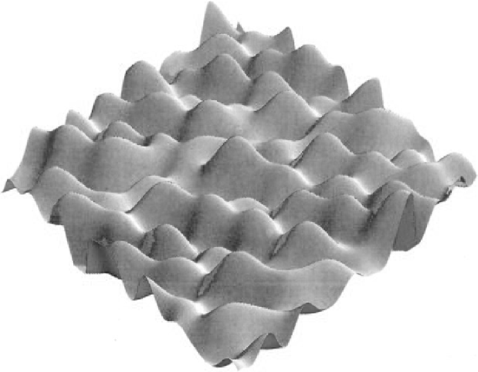
Figure 1: The string theory landscape. The vertical axis represents the value of potential energy density (or equivalently, the cosmological constant), and the two horizontal directions represent two out of hundreds of directions in parameter space, which characterize each vacuum solution. Each valley represents a metastable vacuum solution which may have negative, zero or positive cosmological constant.

Most of these bubbles will never be hospitable to life. For example, bubbles with large positive cosmological constant do not allow for structures such as galaxies or atoms to form Weinberg87 ; Linde87 . And bubbles with large negative cosmological constant collapse long before life has a chance to evolve. However, because the landscape of possibilities is so large, there will also be many bubbles which do provide a suitable environment for life to flourish. Obviously we live in one of these “friendly” bubbles.

In the framework of the multiverse, some physical parameters that were once thought of as fundamental universal parameters get demoted to local environmental parameters. We no longer expect to calculate the “constants” from first principles. Instead we are compelled to calculate how the “constants” are distributed throughout the multiverse. If we assume we are a typical civilization, we should expect to observe values near the peak of the distribution AV95 .

The multiverse paradigm has led to the successful so-called anthropic prediction of the cosmological constant Weinberg87 ; Linde87 ; AV95 ; Efstathiou ; MSW ; GLV ; Bludman ; AV05 . Theoretically we expect the magnitude of the cosmological constant $\Lambda\sim 1$, but the observed value is $\Lambda_{0}\sim 10^{-120}$. This has been one of the biggest problems in theoretical physics.

The probability for a randomly picked observer to measure a given value of $\Lambda$ can be expressed as AV95

$$P_{\text{obs}}(\Lambda)\propto P(\Lambda)n_{\text{obs}}(\Lambda),$$ (1)

where $P(\Lambda)$ is the volume fraction of regions with a given value of $\Lambda$ and $n_{\text{obs}}(\Lambda)$ is the number of observers per unit thermalized volume.

The factor $n_{\text{obs}}(\Lambda)$ takes into account selection effects and is sometimes called the anthropic factor. It is in general very difficult to calculate. However, it has been shown Weinberg87 that the function $n_{\text{obs}}(\Lambda)$ is only substantially different from zero in a tiny window of width

$$\Delta\Lambda_{A}\sim 100\Lambda_{0}\sim 10^{-118}$$ (2)

around $\Lambda=0$. $\Delta\Lambda_{A}$ is sometimes called the Weinberg window or the anthropic range.

The volume factor $P(\Lambda)$ depends on the dynamics of eternal inflation and on the underlying fundamental theory. However, it has been argued AV96 ; Weinberg96 that it should be accurately approximated by a flat distribution,

$$P(\Lambda)\approx{\rm const}$$ (3)

because the anthropic range (2) is vastly less than the expected Planck scale range of variation of $\Lambda$. A smooth function varying on this large characteristic scale will be nearly constant within the minute anthropic interval.

A tiny non-zero value for $\Lambda$ was predicted Weinberg87 ; Linde87 ; AV95 ; BP when the theoretical vogue was to believe that a deep symmetry forced the cosmological constant to be zero. One should keep in mind, however, that the successful anthropic prediction for $\Lambda$ depends critically on the assumption of a flat volume distribution (3).

In SPV we used the new prescription introduced in GSPVW to calculate bubble abundances in an eternally inflating spacetime to actually calculate the volume distribution for the cosmological constant $\Lambda$ in the context of the Bousso-Polchinski (hereafter BP) landscape model. We found that the resulting distribution has a staggered appearance, in conflict with the heuristically expected flat distribution.

One might think that the staggered distribution is a feature of the BP model. However, in this paper we calculate the volume distribution for $\Lambda$ in a simpler landscape model proposed by Arkani-Hamed, Dimopolous and Kachru AHDK (hereafter called the ADK model) and once again find a wildly varying distribution for $\Lambda$.

The outline of this paper is as follows: In section II we will describe the ADK landscape model. In section III we use the new prescription GSPVW for calculating probabilities to calculate the volume distribution for $\Lambda$ in the ADK model. We will conclude with a discussion in section IV.

II The ADK landscape

Following Ref. AHDK we consider a single scalar field $\phi$ with a general quartic potential. Also we assume that the theory has two minima at $\phi_{\pm}$ with vacuum energies $V_{\pm}$, and we take $V_{+}\geq V_{-}$. Thus $V_{+}$ ($V_{-}$) represents the energy of the false vacuum (true vacuum) at $\phi_{+}$ ($\phi_{-}$)(see Fig. 2). We can label the vacua by $\eta=\pm 1$, and define

$$V_{\eta}=V_{av}+\eta V_{\text{dif}}$$ (4)

with

$$V_{av}={\frac{1}{2}}(V_{+}+V_{-})$$ (5)

and

$$V_{\text{dif}}={\frac{1}{2}}(V_{+}-V_{-})$$ (6)

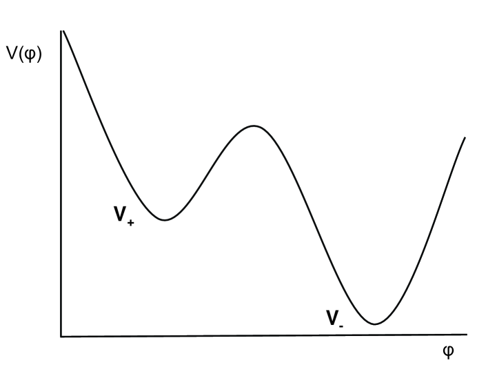
Figure 2: Potential with two metastable minima.

Now consider a theory with J scalar fields $\phi_{a}$, $a=1,...,J$, each having independent quartic potentials $V_{a}(\phi_{a})$ such that the potential is the sum of $J$ independent potentials

$$V=\sum_{a=1}^{J}V_{a}(\phi_{a})$$ (7)

This theory represents a landscape of $2^{J}$ vacua labeled by $\{\eta\}=\{\eta_{1},...,\eta_{J}\}$ with $\eta_{a}=\pm 1$.

The cosmological constant is given by

$$\Lambda_{\{\eta\}}=\bar{\Lambda}+\sum_{a=1}^{J}\eta_{a}V_{{\text{dif}}~{}a}$$ (8)

where

$$\bar{\Lambda}=\sum_{a=1}^{J}V_{{av~{}}a}=J\bar{V}_{av~{}}$$ (9)

If we consider a specific bubble which is completely specified by $\{\eta_{1},...,\eta_{a},...\eta_{J}\}$, the field configuration in an inflating region can change to $\{\eta_{1},...,\eta_{a}\pm 2,...\eta_{J}\}$ when one of the fields $\phi_{a}$ tunnels to its other minimum through bubble nucleation. Thus, as in the BP model, the universe can start off with an arbitrary large cosmological constant, and then diffuse through the ADK landscape of possible vacua as bubbles nucleate one within the other.

ADK asked the question, does a landscape with $2^{J}$ vacua guarantee that we can solve the cosmological constant problem? In the ADK model the histogram of the number of vacua per bin of $\Lambda$ is well approximated by a Gaussian distribution because $\Lambda$ is the sum of many independent components. If $\Lambda=0$ is on the tail of the Gaussian the cosmological constant will not scan around $0$, but if it is near the peak we can expect to find a dense enough spectrum of vacua to account for $\Lambda_{0}$. Thus ADK concluded that for the landscape to solve the cosmological constant problem, either a tiny cosmological constant can accidentally arise on the tail of the Gaussian or the Gaussian must be peaked close enough to $\Lambda=0$.

We wish to point out that even if the Gaussian is peaked around $\Lambda=0$, yielding a sufficiently dense spectrum of $\Lambda$ in the anthropic range $\Delta\Lambda_{A}$, this is still not good enough to validate the anthropic resolution of the cosmological constant problems. It could be that the probabilities of these anthropic vacua differ dramatically (we have learned from our calculation in the BP model SPV that the probabilities tend to span many orders of magnitude) with one or two dominating the distribution.

We will now calculate the volume distribution $P(\Lambda)$ for the ADK model.

III Probabilities in the ADK landscape

In this section we study the volume distribution for $\Lambda$ in the ADK landscape using the prescription of GSPVW which we outline below. We expect to find a wildly varying distribution like the one found for the BP model studied in SPV .

III.1 Summary of probability prescription

Suppose we have a theory with a discrete set of vacua, labeled by index $j$, and having cosmological constants $\Lambda_{j}$. The volume distribution is given by GSPVW

$$P_{j}\propto p_{j}Z_{j}^{3},$$ (10)

where $p_{j}$ is the relative abundance of bubbles of type $j$ and $Z_{j}$ is (roughly) the amount of slow-roll inflationary expansion inside the bubble after nucleation (so that $Z_{j}^{3}$ is the volume slow-roll expansion factor).

The bubble abundances $p_{j}$ can be related to the comoving volume fractions $f_{j}(t)$ which obey the evolution equation recycling

$${df_{j}\over{dt}}=\sum_{i}(-\kappa_{ij}f_{j}+\kappa_{ji}f_{i}),$$ (11)

where the first term on the right-hand side accounts for loss of comoving volume due to bubbles of type $i$ nucleating within those of type $j$, and the second term reflects the increase of comoving volume due to nucleation of type-$j$ bubbles within type-$i$ bubbles.

The transition rate $\kappa_{ij}$ is defined as the probability per unit time for an observer who is currently in vacuum $j$ to find herself in vacuum $i$ and is given by

$$\kappa_{ij}=\Gamma_{ij}{4\pi\over{3}}H_{j}^{-4},$$ (12)

where $\Gamma_{ij}$ is the bubble nucleation rate per unit physical spacetime volume (same as $\lambda_{ij}$ in GSPVW ) and

$$H_{j}=(\Lambda_{j}/3)^{1/2}$$ (13)

is the expansion rate in vacuum $j$.

Eq. (11) can be written in a vector form,

$${d{\bf f}\over{dt}}={\mathbf{M}}{\bf f},$$ (14)

where ${\bf f(t)}\equiv\{f_{j}(t)\}$ and

$$M_{ij}=\kappa_{ij}-\delta_{ij}\sum_{r}\kappa_{ri}.$$ (15)

Let’s label the eigenvalue (of the transition matrix ${\mathbf{M}}$) which has the smallest negative real part (in magnitude), $-q$, and the corresponding eigenvector, $\mathbf{s}$. Then it can be shown that the bubble abundances $p_{j}$ are given by

$$p_{j}\propto\sum_{\alpha}H_{\alpha}^{q}\kappa_{j\alpha}s_{\alpha}.$$ (16)

where the summation is over all recyclable vacua which can directly tunnel to $j$.

The problem of calculating $p_{j}$ has thus been reduced to finding the dominant eigenvalue $q$ and the corresponding eigenvector ${\bf s}$ of the transition matrix $\mathbf{M}$. To calculate the elements of $\mathbf{M}$ we need to calculate the bubble nucleation rates specific to the landscape model we are studying.

III.2 Nucleation rates in the ADK landscape

Transitions between neighboring vacua, which change one of the integers $\eta_{a}$ by $\pm 2$ can occur through bubble nucleation. The bubbles are bounded by thin branes, with tension $\tau_{a}$. By analogy with the BP model we will take the brane tension in the ADK model to be

$$\tau_{a}\equiv\sqrt{\Delta\Lambda_{a}}=\sqrt{2V_{\text{dif},a}}$$ (17)

Transitions with multiple brane nucleation, in which several $\eta_{a}$ are changed at once, are likely to be strongly suppressed Megevand , and we shall disregard them here.

The bubble nucleation rate $\Gamma_{ij}$ per unit spacetime volume can be expressed as CdL

$$\Gamma_{ij}=A_{ij}\exp^{-B_{ij}}$$ (18)

with

$$B_{ij}=I_{ij}-S_{j}$$ (19)

Here, $I_{ij}$ is the Coleman-DeLuccia instanton action and

$$S_{j}=-{8\pi^{2}\over{H_{j}^{2}}}$$ (20)

is the background Euclidean action of de Sitter space with expansion rate

$$H_{j}=\sqrt{\Lambda_{j}/3}.$$ (21)

In the relevant case of a thin-wall bubble, the instanton action $I_{ij}$ has been calculated in Refs. CdL ; BT . It depends on the values of $\Lambda$ inside and outside the bubble and on the brane tension $\tau$.

Let us first consider a bubble which changes one $\eta_{a}$ from $\eta_{a}=+1$ to $\eta_{a}=-1$. The resulting change in the cosmological constant is given by

$$|\Delta\Lambda_{a}|=2V_{\text{dif},a}$$ (22)

and the exponent in the tunneling rate (18) can be expressed as

$$B_{a\downarrow}=B_{a\downarrow}^{flatspace}r(x,y).$$ (23)

$B_{a\downarrow}^{flatspace}$ is the flat space bounce action,

$$B_{a\downarrow}^{flatspace}=\frac{27\pi^{2}}{2}\frac{\tau_{a}^{4}}{|\Delta\Lambda_{a}|^{3}}.$$ (24)

With the aid of Eqs. (17),(22) it can be expressed as

$$B_{a\downarrow}^{flatspace}=\frac{27\pi^{2}}{4V_{\text{dif},a}}$$ (25)

The gravitational correction factor $r(x,y)$ is given by Parke

$$r(x,y)=\frac{2[(1+xy)-(1+2xy+x^{2})^{\frac{1}{2}}]}{x^{2}(y^{2}-1)(1+2xy+x^{2})^{\frac{1}{2}}}$$ (26)

with the dimensionless parameters

$$x\equiv\frac{3\tau_{a}^{2}}{4|\Delta\Lambda_{a}|}=\frac{3}{4}$$ (27)

and

$$y\equiv\frac{2\Lambda}{|\Delta\Lambda_{a}|}-1,$$ (28)

where $\Lambda$ is the background value prior to nucleation.

The prefactors $A_{ij}$ in (18) can be estimated as Jaume

$$A_{ij}\sim 1$$ (29)

If the vacuum $\{\eta_{1}...\eta_{a-1},\eta_{a}-2,\eta_{a+1}....\}$ still has a positive energy density, then an upward transition from $\{\eta_{1}...\eta_{a-1},\eta_{a}-2,\eta_{a+1}....\}$ to $\{\eta_{1}...\eta_{a-1},\eta_{a},\eta_{a+1}....\}$ is also possible. The corresponding transition rate is characterized by the same instanton action and the same prefactor EWeinberg , and it follows from Eqs. (18), (19) and (21) that the upward and downward nucleation rates are related by

$$\Gamma_{ji}=\Gamma_{ij}\exp\left[-24\pi^{2}\left(\frac{1}{\Lambda_{i}}-\frac{1}{\Lambda_{j}}\right)\right]$$ (30)

where $\Lambda_{j}>\Lambda_{i}$. As expected the transition rate from $\eta_{a}=-1$ up to $\eta_{a}=+1$ is suppressed relative to that from $\eta_{a}=+1$ down to $\eta_{a}=-1$. The closer we are to $\Lambda_{i}=0$, the more suppressed are the upward transitions $i\to j$ relative to the downward ones.

We will now investigate the dependence of the tunneling exponent $B_{a\downarrow}$ on the parameters of the model in the limits of small and large $\Lambda$. For $\Lambda\ll|\Delta\Lambda_{a}|$, we have $y\approx-1$, and Eq. (26) gives

$$r(y\to-1)=16.$$ (31)

The inclusion of gravity increases the tunneling exponent causing a suppression of the nucleation rate.

In the opposite limit, $\Lambda\gg|\Delta\Lambda_{a}|$, $y\gg 1$,

$$r(y\gg 1)\approx\sqrt{2}(xy)^{-3/2},$$ (32)

and

$$B_{a\downarrow}\approx 27\pi^{2}\sqrt{V_{\text{dif},a}}\left(\frac{2}{3\Lambda}\right)^{3/2}.$$ (33)

For large values of $\Lambda$, $r\ll 1$, so the nucleation rate is enhanced. The tunneling action must always be large enough to justify the use of the semi-classical approximation: $B_{a\downarrow}\gg 1$, or

$$\Lambda\ll 30V_{\text{dif},a}^{1/3}.$$ (34)

If $V_{\text{dif},a}$ and $\Lambda$ are changed simultaneously, keeping the ratios $\Lambda/V_{\text{dif},a}$ fixed, then $x$ and $y$ do not change, and it is clear from Eqs. (23),(25),(26) that the nucleation exponents scale as $B_{ij}\propto\Lambda^{-1}$. This shows that bubble nucleation rates are strongly suppressed when the energy scales of $V_{\text{dif},a}$ and $\Lambda$ are well below the Planck scale.

III.3 Bubble abundances in the ADK model

We will calculate the bubble abundances for a $J=10$ ADK model, containing $2^{10}$ vacua, with parameter values:

$$V_{\text{dif},a}=\{0.0514,0.0814,0.0885,0.1081,0.1378,0.1475,0.1790,0.2226,0.2467,0.2523\}$$ (35)

and $\bar{\Lambda}=0$. A histogram of the number of vacua vs. $\Lambda$ for this model is given in Fig. 3.

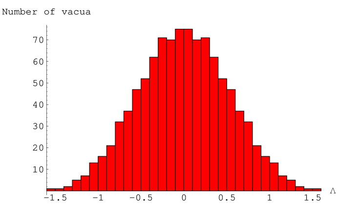
Figure 3: The spectrum of vacua for a $J=10$ ADK landscape with parameters given in Eq. (35)

In direct analogy with our calculation of probabilities for the BP landscape SPV , we resort to perturbative techniques, where we use the smallness of upward transitions as a small parameter. The slowest vacuum to decay was singled out as the dominant vacuum $\alpha_{*}$. To zero’th order in perturbation theory (hereafter PT) the only vacua which aquire non-zero probabilities are those that are direct offspring from the dominant vacuum $\alpha_{*}$. These vacua will have large negative cosmological constants.

The results for the first order bubble abundance factors $p_{j}$ are shown in Fig.4.

Figure 4: Plot of $\log_{10}(1/p_{j})$ vs. $\Lambda_{j}$ for the ADK model with parameters given in (35) and $x=3/4$ (see (27)). The star marks the dominant vacuum $\alpha_{*}$.

The dominant site in Fig. 4 has “coordinates” (-1, 1, -1, 1, 1, -1, 1, -1, -1, 1) and has a very small cosmological constant $\Lambda_{*}=0.0019$. The five squares represent the vacua which can be reached from $\alpha_{*}$ via one upward jump. Their bubble abundances are so low because $\Lambda_{*}$ is so small resulting in very suppressed upward jumps (see Eq. (30)). Each site represented by a square can then jump down in 5 ways (excluding jumps back to the dominant site itself) to the sites depicted as triangles which can in turn jump down to the circles followed by crosses.

The probabilities $p_{j}$ shown here are more suppressed than the BP results in SPV because $\Lambda_{*}$ happens to be much smaller. This is simply a consequence of the different parameters. Also, unlike the BP results, it appears as though vacua which result from downward jumps from a given up jump, have almost the same probability. This “flatness” is fictitious - there are actually a few orders of magnitude difference amongst these vacua which is hard to see graphically because of the scale. However, overall the “staggered” nature of the distribution is evident and the similarity to the BP model is clear.

In addition to the bubble abundance factor $p_{j}$, the volume distribution (10) includes the slow-roll expansion factor $Z_{j}$. There is no reason to expect the expansion factor to tame the wildly varying bubble abundance distribution, and thus we conclude that the volume distribution for $\Lambda$ will have the same form as that calculated for the bubble abundances.

IV Conclusions and Discussion

In SPV we found that for the Bousso-Polchinski string theory landscape, the cosmological constant probability distribution varies dramatically for vacua which have close values of $\Lambda$. We have shown that this behavior persists in the case of the Arkani-Hamed-Dimopolous-Kachru landscape model.

This result was expected. Our probability prescription picks a dominant vacuum and all other vacua are reached from it via a sequence of upward and downward jumps. To zero’th order in PT only the progeny of the dominant vacuum have non-zero probabilities. These vacua were shown to have large negative $\Lambda$. To the first order in PT only a small subset of vacua related to the dominant site via one upward jump and any number of downward jumps gain non-zero probabilities. The probabilities of these vacua are proportional to the tunneling transition rates of the jumps. The tunneling transition rates have an exponential dependence on the parameters of the theory and consequently the probabilities span many orders of magnitude, in both landscape models considered.

Furthermore, it is exceedingly unlikely that one of these first order vacua should be in the anthropic range - we just don’t have enough of them. So what happens if we go to second order in PT?

Calculations indicate that vacua which can be reached via two upward jumps and subsequent downward jumps would gain some tiny probabilities. There would be many more vacua which can be reached via paths including two upward jumps instead of only one, but we would still need to consider higher and higher orders of PT before a sufficient fraction of the theory’s vacua can be infused with probability. Going to higher orders is technically prohibitive.

Although the distributions we have calculated do not give a flat distribution to first order, we cannot conclude that the anthropic prediction of the cosmological constant was a fluke. The distributions we are able to calculate are simply the tip of the iceberg. It is still entirely possible that vacua in the anthropic range are smoothly distributed.

So how do we proceed from here? How do we look beyond the first order results we have found for a tiny subset of vacua in our landscape? Currently we do not have a definitive answer to this question. But work is underway to try to elucidate what essential features of a given landscape model will guarantee that (once we have many vacua in the anthropic range) a sufficient number of the most probable anthropic vacua will have close enough probabilities to ensure that the distribution can be considered to be smooth.

V Acknowledgements

I would like to thank Ken Olum and Alex Vilenkin for their support and also for many useful suggestions for this manuscript.

References

- (1) A. Vilenkin, Phys. Rev. D27, 2848-2855 (1983).
- (2) A. D. Linde, Mod. Phys. Lett. A1, 81 (1986); A. D. Linde, Phys. Lett. 175B, 395-400 (1986); A.S. Goncharov, A. D. Linde, and V. F. Mukhanov, Int. J. Mod. Phys. A2, 561-591 (1987).
- (3) A. Starobinsky, in Field Theory, Quantum Gravity and Strings, eds: H. J. de Vega and N. Sánchez, Lecture Notes in Phyics (Springer Verlag) Vol. 246, pp. 107-126 (1986).
- (4) R. Bousso and J. Polchinski, JHEP 0006, 006 (2000).
- (5) L. Susskind, “The anthropic landscape of string theory,” arXiv:hep-th/0302219.
- (6) M. J. Duff, B. E. W. Nilsson, and C. N. Pope, Phys. Rept. 130, 1 (1986).
- (7) S. Coleman and F. DeLuccia, Phys. Rev. D21, 3305 (1980).
- (8) S. Parke, “Gravity and the decay of the false vacuum”, Phys. Letters B 121 (1983) 313.
- (9) J. D. Brown and C. Teitelboim, Phys. Lett. B195, 177 (1987); Nucl. Phys. B297, 787 (1988).
- (10) K. M. Lee and E. J. Weinberg, Phys. Rev. D 36, 1088 (1987).
- (11) J. Garriga and A. Vilenkin, Phys. Rev. D57, 2230 (1998).
- (12) S. Weinberg, Phys. Rev. Lett. 59, 2607 (1987).
- (13) A.D. Linde, in 300 Years of Gravitation, ed. by S.W. Hawking and W. Israel, (Cambridge University Press, Cambridge, 1987).
- (14) A. Vilenkin, Phys. Rev. Lett. 74, 846 (1995).
- (15) G. Efstathiou, M.N.R.A.S. 274, L73 (1995).
- (16) H. Martel, P. R. Shapiro and S. Weinberg, Ap.J. 492, 29 (1998).
- (17) J. Garriga, M. Livio and A. Vilenkin, Phys. Rev. D61, 023503 (2000).
- (18) S. Bludman, Nucl. Phys. A663-664,865 (2000).
- (19) For a review, see, e.g., A. Vilenkin, “Anthropic predictions: the case of the cosmological constant”, astro-ph/0407586.
- (20) A. Vilenkin, in Cosmological Constant and the Evolution of the Universe, ed by K. Sato, T. Suginohara and N. Sugiyama (Universal Academy Press, Tokyo, 1996).
- (21) S. Weinberg, in Critical Dialogues in Cosmology, ed. by N. G. Turok (World Scientific, Singapore, 1997).
- (22) D. Schwartz-Perlov and A. Vilenkin, “Probabilities in the Bousso-Polchinski multiverse”, JCAP 0606:010, 2006, hep-th/0601162.
- (23) J. Garriga, D. Schwartz-Perlov, A. Vilenkin and S. Winitzki, “Probabilities in the inflationary multiverse”, hep-th/0509184.
- (24) N. Arkani-Hamed, S. Dimopoulos and S. Kachru, “Predictive landscapes and new physics at a TeV”, arXiv:hep-th/0501082.
- (25) J. Garriga and A. Megevand, Phys. Rev. D69, 083510 (2004).
- (26) J. Garriga, Phys. Rev. D 49 (1994) 6327.
- (27) R. Easther, E.A. Lim and M.R. Martin, “Counting pockets with world lines in eternal inflation”, arXiv:astro-ph/0511233.