Gravitational spectrum of black holes in the Einstein-Aether theory.

Abstract

Evolution of gravitational perturbations, both in time and frequency domains, is considered for a spherically symmetric black hole in the non-reduced Einstein-Aether theory. It is shown that real oscillation frequency and damping rate are larger for the Einstein-Aether black hole than for the Schwarzschild black hole. This may provide an opportunity to observe aether in the forthcoming experiments with new generation of gravitational antennas.

One of the most intriguing issues of modern physics consists in attempts to go beyond local Lorentz symmetry LV . In theory of gravity, breaking of local Lorentz invariance leads to a general relativity coupled to a dynamical time-like vector field $u^{a}$, called “aether”. More exactly, $u^{a}$ breaks local boost invariance, while rotational symmetry in a preferred frame is preserved AEreview . Thereby, aether is a kind of locally preferred state of rest at each point of space-time due-to some unknown physics. Recently observable consequences of Einstein-Aether theory attracted considerable interest AEobserve . Gravitational consequences of Local Lorentz symmetry violation must show themselves in radiative processes around black holes. It is known that gravitational radiation damping of binary pulsars orbits reproduces the weak field general relativity at lowest post- Newtonian order Foster . Yet, the significant difference between Einstein and Einstein-Aether theories should be seen in the regime of strong field, for instance in observing of the characteristic quasi-normal spectrum of black holes. Thus, existence of aether could be tested in the forthcoming experiments with new generation of gravitational antennas. Motivated by the above reasons, in a previous letter Konoplya-Zhidenko-PLB2 we developed a method for finding of the quasinormal modes for the perturbations of metrics which are not known analytically, but instead are given only numerically in some region near black holes. That is the case of the Einstein-Aether black holes found in Jacobson . In Konoplya-Zhidenko-PLB2 , there were found the quasinormal modes for test scalar and electromagnetic fields in the vicinity of the Einstein-Aether black holes. It was shown that the scalar and electromagnetic quasinormal modes in the Einstein-Aether theory, have larger real oscillation frequency and damping rate than those of the Schwarzschild black holes in the Einstein theory. As quasinormal spectrum does not depend on the spin of the field in eikonal regime, qualitatively the same QN behavior was suggested in Konoplya-Zhidenko-PLB2 for the gravitational perturbations as for scalar and electromagnetic ones. In the present work we show that it is indeed true, and analyze gravitational perturbations of the Einstein-Aether black holes both in frequency and time domain.

We shall start from the lagrangian of the full Einstein-Aether theory forms the most general diffeomorphism invariant action of the space-time metric $g_{ab}$ and the aether field $u^{a}$ involving no more than two derivatives given by

$$L=-R-K^{ab}_{\leavevmode\nobreak\ \leavevmode\nobreak\ \leavevmode\nobreak\ mn}\nabla_{a}u^{m}\nabla_{b}u^{n}-\lambda(g_{ab}u^{a}u^{b}-1),$$ (1)

here $R$ is the Ricci scalar, $\lambda$ is a Lagrange multiplier which provides the unit time-like constraint,

$$K^{ab}_{\leavevmode\nobreak\ \leavevmode\nobreak\ \leavevmode\nobreak\ mn}=c_{1}g^{ab}g_{mn}+c_{2}\delta^{a}_{m}\delta^{b}_{n}+c_{3}\delta^{a}_{n}\delta^{b}_{m}+c_{4}u^{a}u^{b}g_{mn},$$

where the $c_{i}$ are dimensionless constants.

Spherically symmetry allows to fix $c_{4}=0$. In this letter, following Jacobson , we shall consider the so-called non-reduced Einstein-Aether theory, for which $c_{3}=0$, and we can use the field redefinition that fixes the coefficient $c_{2}$ Jacobson :

$$c_{2}=-\frac{c_{1}^{3}}{2-4c_{1}+3c_{1}^{2}},$$

so that $c_{1}$ is the free parameter.

The metric for a spherically symmetric static black holes in Eddington-Finkelstein coordinates can be written in the form Jacobson :

$$ds^{2}=N(r)dv^{2}-2B(r)dvdr-r^{2}d\Omega^{2},$$ (2)

where the functions $N(r)$ and $B(r)$ are given by numerical integration near the black hole event horizon Jacobson . One can re-write this metric in a Schwarzschild like form:

$$ds^{2}=-N(r)dt^{2}+\frac{B^{2}(r)}{N(r)}dr^{2}+r^{2}d\Omega^{2}.$$ (3)

Since the background value of aether coupling, determined by constants $c_{i}$ is small in comparison with the background characteristics of large black hole, determined by the mass of the black hole $M$. Therefore, the background black hole metric is, in fact, the Schwarzschild metric slightly corrected by the aether. Thus, one can neglect small perturbations of aether, keeping only linear perturbations of Ricci tensor. Then the perturbation equations with unperturbed aether have the form:

$$\delta R_{\alpha\beta}=0.$$ (4)

The general form of the perturbed metric, according to Chandrasekhar designations, is

$$ds^{2}=e^{2\nu}dt^{2}-e^{2\psi}(d\phi^{2}-\omega dt-q_{2}dr-q_{3}d\theta)^{2}-$$

$$e^{-2\mu_{2}}dr^{2}-e^{-2\mu_{3}}d\theta^{2}.$$ (5)

Here

$$e^{2\nu}=N(r),\quad e^{2\mu_{2}}=N(r)/B^{2}(r),$$

$$e^{2\mu_{3}}=r^{2},\quad e^{2\psi}=r^{2}\sin^{2}\theta.$$ (6)

Let us introduce new variables

$$Q_{ik}=q_{i,k}-q_{k,i},\quad Q_{i0}=q_{i,0}-\omega_{,i},\quad i,k=2,3.$$ (7)

Here we used $0,1,2,3$ for $t$, $\phi$, $r$ and $\theta$ coordinates respectively. Here we shall consider the axial type of gravitational perturbations. The equations (11),(12) on p.143 of Chandra can be reduced to a single equation

$$\frac{r^{4}}{B}\left(\frac{N}{Br^{2}}\frac{\partial Q}{\partial r}\right)_{,r}-\frac{r^{2}}{B}\frac{\partial^{2}Q}{\partial t^{2}}+\sin^{3}\theta\frac{\partial}{\partial\theta}\left(\frac{1}{sin^{3}\theta}\frac{\partial Q}{\partial\theta}\right)=0$$ (8)

where we used

$$Q=e^{3\psi+\nu-\mu_{2}-\mu_{3}}Q_{23}.$$ (9)

The following representation of the function $Q(t,r,\theta)$

$$Q(t,r,\theta)=rR_{\ell}(t,r)C_{\ell+2}^{-3/2}(\theta)$$ (10)

leads to separation of angular variable $\theta$.

Finally we have the wave-like equation for the radial coordinate

$$\frac{d^{2}\Psi}{dr_{*}^{2}}+(\omega^{2}-V(r))\Psi=0,\qquad dr_{*}=\frac{B(r)}{N(r)}dr.$$ (11)

with the effective potential

$$V(r)=N(r)\frac{(\ell+2)(\ell-1)}{r^{2}}+\frac{2N^{2}(r)}{B^{2}(r)r^{2}}-\frac{1}{r}\frac{d(N(r)/B(r))}{dr^{*}}.$$ (12)

Quasi-normal modes of asymptotically AdS black holes have been studies recent years extensively, because of their interpretation in Conformal Field Theory CFT with some specific boundary conditions. In astrophysically relevant problem, one should require natural boundary conditions for QN modes of purely in-going waves at the event horizon and purely out-going waves at spatial infinity

$$\Psi\sim e^{\pm ir_{*}\omega}\quad r_{*}\rightarrow\pm\infty.$$ (13)

Under these boundary conditions, the quasinormal modes were studied in a great number of papers QNMs , yet in those cases the background metric and the effective potential were known in analytical form. For the case of Einstein-Aether theory, we are in position to apply the method developed in our previous paper Konoplya-Zhidenko-PLB2 . Here we shall give only a brief summary of the whole procedure of Konoplya-Zhidenko-PLB2 .

We approximate the numerical data for the metric by a fit of the form

$$N(r)=\frac{\displaystyle\sum_{i=0}^{N_{N}}a^{(N)}_{i}r^{i}}{\displaystyle 1+\sum_{i=1}^{N_{N}}b^{(N)}_{i}r^{i}},\quad B(r)=\frac{\displaystyle\sum_{i=0}^{N_{B}}a^{(B)}_{i}r^{i}}{\displaystyle 1+\sum_{i=1}^{N_{B}}b^{(B)}_{i}r^{i}}.$$

which are substituted into equations (11) and (12). The numbers $N_{N}$ and $N_{B}$ determine the number of terms in the polynomials and are chosen in order to provide best convergence of the WKB series. Coefficients $a^{(N)}_{i}$, $b^{(N)}_{i}$, $a^{(B)}_{i}$, $b^{(B)}_{i}$ are determined by the fitting procedure. The WKB expansion has the form

$$\frac{\imath Q_{0}}{\sqrt{2Q_{0}^{\prime\prime}}}-\sum_{i=2}^{6}\Lambda_{i}=n+\frac{1}{2},$$ (14)

where the correction terms of the i-th WKB order $\Lambda_{i}$ can be found in WKB ; Will-Schutz and Konoplya-prd3 , $Q=V-\omega^{2}$ and $Q_{0}^{i}$ means the i-th derivative of $Q$ at its maximum.

Alternatively, we shall use the above mentioned fits of the metric functions, and consequently of the effective potential, in the time-domain analysis: using the integration scheme described for instance in Price-Pullin . In detail, we used a numerical characteristic integration scheme, based in the light-cone variables $u=t-r_{\star}$ and $v=t+r_{\star}$. In the characteristic initial value problem, initial data are specified on the two null surfaces $u=u_{0}$ and $v=v_{0}$. The discretization scheme applied, is

$$\Psi(N)=\Psi(W)+\Psi(E)-\Psi(S)$$ (15)

$$\mbox{}-\Delta^{2}V(S)\frac{\Psi(W)+\Psi(E)}{8}+\mathcal{O}(\Delta^{4})\ ,$$

where we have used the definitions for the points: $N=(u+\Delta,v+\Delta)$, $W=(u+\Delta,v)$, $E=(u,v+\Delta)$ and $S=(u,v)$.

The application of the above two methods shows excellent agreement: for instance the fundamental mode $0.7686-0.1887i$ in time domain is very close to the WKB value $0.769470-0.187783i$ for $c_{1}=0.4$, as can be seen in Fig. 2. From the obtained numerical data in Table I and time domain pictures in Fig. 1-2, one can see that when increasing $c_{1}$, both real oscillation frequency and damping rate are increasing. Even for a small aether $c_{1}\sim 0.1$, the increase in $Re\omega$ and $Im\omega$ is of about half percent, and could, in principle, be detected by new generation of gravitational antennas. For larger $c_{1}$, the difference between, Schwarzschild and Einstein-Aether QNMs can be very significant and reach six-seven percents. From the Table I, it is evident that both real and imaginary parts of $\omega$ grows when increasing the multipole number $\ell$. Here we considered only axial gravitational perturbations, which are iso-spectral with polar gravitational perturbations for Schwarzschild black holes. For black holes in Einstein-Aether theory this iso-spectrality will be broken, and QNMs for polar perturbations should slightly differ from axial, when considering the full perturbations of Einstein-Aether equations. The same breaking of iso-spectrality happens, for instance, when perturbing dilaton black holes or black holes in higher than four dimensional space-times Konoplya:2003dd . In our approach, the perturbations of aether were neglected in comparison with perturbations of the metric of a large astrophysical black hole. Therefore this difference between axial and polar QN spectra was neglected as well.

Note that we used here the method based on the supposition that QN frequencies are determined mainly near the peak of the potential barrier, while behavior of the potential barrier far from black hole is not significant. Even despite this idea was inspired by WKB approach, it is not dependent on WKB technique, as was shown here by computations in time domain.

Table 1: Axial gravitational perturbations for the non-reduced Einstein-Aether theory: The fundamental mode.

$c_{1}$	$\ell=2$	$\ell=3$	$\ell=4$	$\ell=5$
$0.1$	$0.751958-0.179578i$	$1.206905-0.187387i$	$1.629395-0.190378i$	$2.038526-0.191824i$
$0.2$	$0.757144-0.180786i$	$1.215669-0.188850i$	$1.641492-0.191932i$	$2.053816-0.193422i$
$0.3$	$0.762871-0.184443i$	$1.225598-0.192601i$	$1.655131-0.195746i$	$2.071021-0.197268i$
$0.4$	$0.769470-0.187783i$	$1.236966-0.196172i$	$1.670792-0.199412i$	$2.090803-0.200981i$
$0.5$	$0.777059-0.192176i$	$1.250474-0.200794i$	$1.689421-0.204151i$	$2.114345-0.205777i$
$0.6$	$0.786784-0.198087i$	$1.267215-0.207061i$	$1.712545-0.210574i$	$2.143595-0.212276i$
$0.7$	$0.799391-0.206961i$	$1.289844-0.216264i$	$1.743878-0.220000i$	$2.183271-0.221813i$
$0.77$	$0.811083-0.216302i$	$1.311449-0.225807i$	$1.773893-0.229784i$	$2.221342-0.231720i$

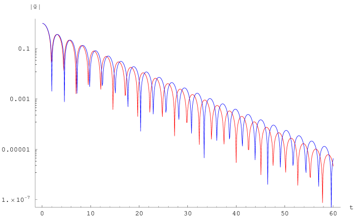
Figure 1: Evolution of axial gravitational perturbations in time domain $c_{1}=0.4$, $\ell=3$, non-reduced theory (red line) in comparison with the Schwarzschild case (blue line).

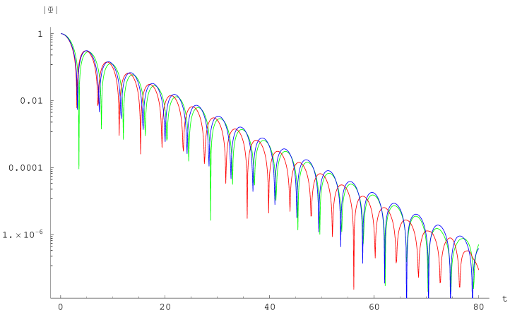
Figure 2: Evolution of axial gravitational perturbations in time domain $c_{1}=0.1$ (green line), $c_{1}=0.4$ (red line), $\ell=2$, non-reduced theory in comparison with the Schwarzschild case (blue line).

- (1) F. Ahmadi, S. Jalalzadeh and H. R. Sepangi, arXiv:gr-qc/0605038; Q. G. Bailey and V. A. Kostelecky, arXiv:gr-qc/0603030; G.L. Alberghi, R. Casadio, A. Tronconi, hep-ph/0310052; V. A. Kostelecky and R. Potting, Gen. Rel. Grav. 37, 1675 (2005) [Int. J. Mod. Phys. D 14, 2341 (2005)] [arXiv:gr-qc/0510124]; B. Altschul, Phys. Rev. D 72, 085003 (2005) [arXiv:hep-th/0507258]; T. G. Rizzo, JHEP 0509, 036 (2005) [arXiv:hep-ph/0506056]; T. Jacobson, S. Liberati and D. Mattingly, Annals Phys. 321, 150 (2006) [arXiv:astro-ph/0505267]; S. Groot Nibbelink and M. Pospelov, Phys. Rev. Lett. 94, 081601 (2005) [arXiv:hep-ph/0404271].
- (2) C. Eling, T. Jacobson and D. Mattingly, arXiv:gr-qc/0410001.
- (3) C. Heinicke, P. Baekler and F. W. Hehl, Phys. Rev. D 72, 025012 (2005) [arXiv:gr-qc/0504005]; M. L. Graesser, A. Jenkins and M. B. Wise, Phys. Lett. B 613, 5 (2005) [arXiv:hep-th/0501223]; R. Bluhm and V. A. Kostelecky, Phys. Rev. D 71, 065008 (2005) [arXiv:hep-th/0412320]; T. Jacobson, S. Liberati and D. Mattingly, Lect. Notes Phys. 669, 101 (2005) [arXiv:hep-ph/0407370]. B. Z. Foster, Phys. Rev. D 73, 024005 (2006) [arXiv:gr-qc/0509121]; B. Z. Foster and T. Jacobson, Phys. Rev. D 73, 064015 (2006) [arXiv:gr-qc/0509083]; C. M. L. de Aragao, M. Consoli and A. Grillo, arXiv:gr-qc/0507048; T. Jacobson and D. Mattingly, Phys. Rev. D 70, 024003 (2004) [arXiv:gr-qc/0402005];
- (4) B. Z. Foster, arXiv:gr-qc/0602004;
- (5) R. A. Konoplya, A. Zhidenko, gr-qc/0605082, Phys. Lett. B, in press
- (6) C. Eling and T. Jacobson, arXiv:gr-qc/0604088; C. Eling and T. Jacobson, arXiv:gr-qc/0603058.
- (7) S. Chandrasekhar, Mathematical Theory of black holes, (Oxford University Press, Oxford, 1983).
- (8) G. T. Horowitz and V. E. Hubeny, Phys. Rev. D 62, 024027 (2000); D. Birmingham, I. Sachs and S. N. Solodukhin, Phys. Rev. Lett. 88, 151301 (2002) [arXiv:hep-th/0112055]; V. Cardoso, R. Konoplya and J. P. S. Lemos, Phys. Rev. D 68, 044024 (2003) [arXiv:gr-qc/0305037]; R. A. Konoplya, Phys. Rev. D 66, 044009 (2002) [arXiv:hep-th/0205142]; V. Cardoso and J. P. S. Lemos, Phys. Rev. D 63, 124015 (2001) [arXiv:gr-qc/0101052].
- (9) A. Lopez-Ortega, arXiv:gr-qc/0605034. P. Kanti and R. A. Konoplya, Phys. Rev. D 73, 044002 (2006) [arXiv:hep-th/0512257]; S. Musiri, S. Ness and G. Siopsis, Phys. Rev. D 73, 064001 (2006) [arXiv:hep-th/0511113]; A. Ghosh, S. Shankaranarayanan and S. Das, Class. Quant. Grav. 23, 1851 (2006) [arXiv:hep-th/0510186]; R. Konoplya, Phys. Rev. D 71, 024038 (2005) [arXiv:hep-th/0410057]; C. G. Shao, B. Wang, E. Abdalla and R. K. Su, Phys. Rev. D 71, 044003 (2005) [arXiv:gr-qc/0410025]; R. A. Konoplya and E. Abdalla, Phys. Rev. D 71, 084015 (2005) [arXiv:hep-th/0503029]. T. Padmanabhan, Class. Quant. Grav. 21, L1 (2004) [arXiv:gr-qc/0310027]; Phys. Rev. D 73, 024009 (2006) [arXiv:gr-qc/0509026]; M. R. Setare Class. Quant. Grav. 21 1453 (2004) [hep-th/0311221]; R. A. Konoplya and A. Zhidenko, Physical Review D73 (2006), 124040, [arXiv:gr-qc/0605013]; S. Fernando, Gen. Rel. Grav. 36, 71 (2004) [arXiv:hep-th/0306214];
- (10) B.F.Schutz and C.M.Will Astrophys.J.Lett 291 L33 (1985);
- (11) S.Iyer and C.M.Will, Phys.Rev. D35 3621 (1987)
- (12) R. A. Konoplya, Phys.Rev D 68, 024018 (2003); R. A. Konoplya, J. Phys. Stud. 8, 93 (2004);
- (13) C. Gundlach, R. H. Price and J. Pullin, Phys. Rev. D 49, 883 (1994); E. Abdalla, R. A. Konoplya and C. Molina, Phys. Rev. D72, 084006 (2005) [arXiv:hep-th/0507100].
- (14) R. A. Konoplya, Phys. Rev. D68, 124017 (2003) [arXiv:hep-th/0309030];