String Tension and String Susceptibility
in two-dimensional generalized Weingarten model

Abstract

We study the two-dimensional generalized Weingarten model reduced to a point, which interpolates between the reduced Weingarten model and the large-$N$ gauge theory. We calculate the expectation value of the Wilson loop using a Monte Carlo method and determine the string tension and string susceptibility. The numerical result suggests that the string susceptibility approaches $-2$ in a certain parametric region, which implies that the branched-polymer configurations are suppressed.

1 Introduction

In this paper, we study a model defined by the action

$$S=-\beta N\sum_{\mu\neq\nu}^{d}\mathrm{Tr}\left(A_{\mu}^{\dagger}A_{\nu}^{\dagger}A_{\mu}A_{\nu}\right)+\alpha N\sum_{\mu=1}^{d}\mathrm{Tr}\left(A_{\mu}^{\dagger}A_{\mu}-1+\frac{1}{\alpha}\right)^{2},$$ (1)

where $A_{\mu}$ $(\mu=1,2,\cdots,d)$ are complex $N\times N$ matrices. (In the actual numerical calculation describe in §  3, we consider only the case $d=2$.) This model interpolates [1] between the reduced Weingarten model [3] and the large-$N$ reduced $U(N)$ gauge theory.[4] We regard the model (1) as describing an ensemble of random surfaces and study whether it can describe the Nambu-Goto string.

The original Weingarten model [5] was proposed as a nonperturbative description of the Nambu-Goto string. This model is defined as follows. Consider a $d$-dimensional square lattice ${\mathbb{Z}}^{d}$ and introduce a complex $N\times N$ matrix $A_{x,\mu}$ for each link connecting the sites $x$ and $x+\hat{\mu}$ in such a way that $A_{x+\hat{\mu},-\mu}=A_{x,\mu}^{\dagger}$. Then the action of the Weingarten model is given by

$$S_{W}=-N\beta\sum_{x}\sum_{\mu\neq\nu}\mathrm{Tr}\left(A_{x,\mu}A_{x+\hat{\mu},\nu}A^{\dagger}_{x+\hat{\nu},\mu}A^{\dagger}_{x,\nu}\right)+N\sum_{x}\sum_{\mu=1}^{d}\mathrm{Tr}\left(A_{x,\mu}^{\dagger}A_{x,\mu}\right).$$ (4)

The partition function is given by

$$Z_{W}=\int dm_{N}\exp\left(-S_{W}\right),$$ (5)

where the measure $dm_{N}$ is defined by

$$dm_{N}=\prod_{x,\mu}\prod_{i,j}\left(\frac{N}{\pi}d\left[{\rm Re}(A_{x,\mu})_{ij}\right]d\left[{\rm Im}(A_{x,\mu})_{ij}\right]\right).$$ (6)

Let $C_{i}$ represent closed contours on the lattice. Then, multiplying $A_{\mu}$ along $C_{i}$ and taking the trace, we obtain Wilson loops $w(C_{i})$. The correlator of $w(C_{i})$, defined by

$$W(C_{1},\cdots,C_{n})=\frac{1}{Z_{W}}\int dm_{N}\exp\left(-S_{W}\right)\frac{1}{N}w(C_{1})\cdots\frac{1}{N}w(C_{n}),$$ (7)

is evaluated as

$$W(C_{1},\cdots,C_{n})=N^{2-2n}\sum_{s\in S(\{C_{i}\})}\exp\left(-a(s)\log\beta^{-1}-h(s)\log N^{2}\right),$$ (8)

where $S(\{C_{i}\})$ is the set of surfaces on the lattice whose boundary is $C_{1}\cup\cdots\cup C_{n}$, $a(s)$ is the area of the surface $s$, and $h(s)$ is the number of handles of $s$. If we regard $\log\beta^{-1}$ and $\frac{1}{N^{2}}$ as the string tension and the string coupling, respectively, then Eq. (8) can be interpreted as the sum of random surfaces weighted by the Nambu-Goto action.

Next, let us consider the reduced Weingarten model [3], whose action is given by

$$S_{RW}=-N\beta\sum_{\mu\neq\nu}\mathrm{Tr}\left(A_{\mu}A_{\nu}A^{\dagger}_{\mu}A^{\dagger}_{\nu}\right)+N\sum_{\mu=1}^{d}\mathrm{Tr}\left(A_{\mu}^{\dagger}A_{\mu}\right).$$ (9)

This action is invariant under the $U(1)^{d}$ transformation

$$A_{\mu}\to e^{i\theta_{\mu}}A_{\mu}.$$ (10)

If this symmetry is not broken spontaneously in the large-$N$ limit, the correlators of the Wilson loops in this model are identical to those of the original Weingarten model, (4). Because the reduced Weingarten model has only $d$ matrices, numerical calculations are more tractable. This model was studied numerically [6] in the cases $d=2,3$, and it was shown that the Weingarten model does not describe smooth surfaces but, rather, branched polymers [7].

One possibility to overcome this difficulty is to consider the modified action (1). This action is motivated by the following observations. First, this model interpolates [1] between the original Weingarten model ($\alpha=0$) and the reduced $U(N)$ gauge theory [4]($\alpha=\infty$). Because both of those models are thought to be related to string theory, it is natural to consider the intermediate region. In this region, this model allows a lattice string interpretation similar to that of the original Weingarten model, because the relation (8) holds also in this model, as long as the surface $s$ does not intersect itself. Second, the action (1) becomes a set of $d$ copies of a complex one-matrix model with a double-well potential. In the case of the Hermitian matrix model, we can describe a type 0B string by flipping the sign of the double-well potential [8]. Therefore we conjecture that also in the case of the Weingarten model, a worldsheet supersymmetry can be introduced by modifying the potential, and this may prevent the worldsheet from becoming branched polymer.

This model has been solved analytically only in the special cases $\beta=0$ [1] and $\alpha=\infty$ for $d=2$.[9, 10] In Ref. HKKK, the parametric region $\alpha\gtrsim 1$ is studied. For sufficiently large $\alpha$, there are $d$ phase transitions that correspond to the partial breakdowns of $U(1)^{d}$ symmetry. For $d\geq 3$, these phase transitions smoothly approach the known phase transitions of the large-$N$ reduced $U(N)$ gauge theory [11, 12] as $\alpha\to\infty$. For sufficiently small $\alpha$ ($\alpha\lesssim 2$ in the case $d=2$), these two transitions seem to occur simultaneously. In this paper, we study the parametric region $\alpha\lesssim 1$ in detail in the case $d=2$. For a technical reason, we study the maximally twisted model.

The organization of this paper is as follows. In § 2, we present theoretical preliminaries. In § 3, we present the numerical result. We study the phase diagram in § 3.1 and then determine the string tension and string susceptibility in § 3.2. Section 4 is devoted to conclusions and discussion of future directions. In Appendix A we comment on numerical results concerning the generalized Weingarten model without a twist.

2 Theoretical preliminaries

2.1 Parametric region of the generalized Weingarten model

We begin by considering the parametric region in which the model defined by the action (1) is well-defined. As shown in REf. [2], the action is bounded from below if and only if

$$\beta\alpha^{-1}\leq\frac{1}{d-1}.$$ (12)

This can be seen as follows. In order to determine whether the action is bounded, it is sufficient to consider the quartic term,

$$S|_{\mathrm{quartic}}=-\beta N\sum_{\mu\neq\nu}^{d}\mathrm{Tr}\left(A_{\mu}^{\dagger}A_{\nu}^{\dagger}A_{\mu}A_{\nu}\right)+\alpha N\sum_{\mu=1}^{d}\mathrm{Tr}\left(A_{\mu}^{\dagger}A_{\mu}A_{\mu}^{\dagger}A_{\mu}\right).$$ (13)

Then, using the inequality

$$2\mathrm{Re}\ \mathrm{Tr}\left(AB^{\dagger}\right)\leq\mathrm{Tr}\left(AA^{\dagger}\right)+\mathrm{Tr}\left(BB^{\dagger}\right),$$ (14)

we have

$$2\mathrm{Re}\ \mathrm{Tr}\left(A_{\mu}A_{\nu}A_{\mu}^{\dagger}A_{\nu}^{\dagger}\right) \leq \mathrm{Tr}\left(A_{\mu}^{\dagger}A_{\mu}A_{\nu}A_{\nu}^{\dagger}\right)+\left(A_{\mu}A_{\mu}^{\dagger}A_{\nu}^{\dagger}A_{\nu}\right)$$ (15)

$$\leq \mathrm{Tr}\left(A_{\mu}^{\dagger}A_{\mu}A_{\mu}^{\dagger}A_{\mu}\right)+\left(A_{\nu}^{\dagger}A_{\nu}A_{\nu}^{\dagger}A_{\nu}\right).$$

Summing over the spacetime subscripts, we obtain

$$\sum_{\mu\neq\nu}^{d}\mathrm{Tr}\left(A_{\mu}^{\dagger}A_{\nu}^{\dagger}A_{\mu}A_{\nu}\right)\leq(d-1)\sum_{\mu=1}^{d}\mathrm{Tr}\left(A_{\mu}^{\dagger}A_{\mu}\right)^{2}.$$ (16)

Combining this relation with (13), we obtain the bound (12). This bound is indeed realized in the case of the unit matrix, for example.

For $\beta\alpha^{-1}>\frac{1}{d-1}$, although the action is not bounded from below, the model still can be well-defined for large-$N$.[3] In the original Weingarten model, the free energy per unit volume, $F(N,\beta)$, is given by

$$\frac{1}{N^{2}}F(N,\beta)=\sum_{g=0}^{\infty}\sum_{A=0}^{\infty}\frac{n_{g}(A)}{N^{2g}}\beta^{A},$$ (17)

where $n_{g}(A)$ represents the number of closed surfaces with genus $g$ and area $A$. By taking the planar limit $N\to\infty$, with $\beta$ kept fixed, we obtain

$$\frac{1}{N^{2}}F(N,\beta)=\sum_{A=0}^{\infty}n_{0}(A)\beta^{A}.$$ (18)

In Refs. EK81 and DFJ83, it is argued that $n_{0}(A)$ behaves as

$$n_{0}(A)\sim A^{b-1}k^{A}$$ (19)

for sufficiently large $A$, where $b$ and $k$ are universal and regularization-dependent constants, respectively. Then, we have

$$\frac{1}{N^{2}}F(N,\beta)\sim\sum_{A=0}^{\infty}A^{b-1}(k\beta)^{A},$$ (20)

and this quantity is finite for $\beta<\beta_{c}=\frac{1}{k}$. In the same way, it can be shown that the expectation value of the Wilson loop is also finite. Therefore, the original Weingarten model is well-defined for $\beta<\beta_{c}$ in the large-$N$ limit.[3]

In numerical simulations, obviously we cannot make $N$ infinite. However, for large enough $N$, there is a metastable state corresponding to the planar limit. The “lifetime” of this metastable state becomes longer as $N$ increases.[6]

For generic $\alpha$, the measure in the strong coupling expansion changes from the Gaussian one in the original Weingarten model as

$$\exp\left(-N\sum_{\mu=1}^{d}\mathrm{Tr}A_{\mu}^{\dagger}A_{\mu}\right)dm_{N}\ \longrightarrow\ \exp\left(-\alpha N\sum_{\mu=1}^{d}\mathrm{Tr}\left(A_{\mu}^{\dagger}A_{\mu}-1+\frac{1}{\alpha}\right)^{2}\right)dm_{N}.$$ (21)

Because we cannot evaluate the strong coupling expansion exactly, we simply assume that the effect of the change of the measure can be absorbed into changes of $b$ and $\beta_{c}$:

$$b,\ \beta_{c}\ \longrightarrow\ b(\alpha),\ \beta_{c}(\alpha).$$ (22)

If this assumption is correct, then the planar limit exists for $\beta<\beta_{c}(\alpha)$ also in this case. As we see in § 3, the numerical data seem to be consistent with this assumption.

2.2 String tension and string susceptibility

First, let us consider the case of the original Weingarten model. Then, the number of planar random surfaces on a lattice with boundary $C$ and area $A$ is given by [13, 14]

$$n_{0}(A;C)\sim A^{b}k^{A}=A^{b}\beta_{c}^{-A}$$ (23)

for large $A$. Note that $n_{0}(A;C)$ is $A$ times larger than $n_{0}(A)$, because there is a degree of freedom corresponding to the choice of the location of a puncture. Then, the expectation value of the Wilson loop is evaluated as

$$W(C) = \sum n_{0}(A;C)\beta^{A}$$ (24)

$$\sim \mbox{const.}\times\sum_{A\geq A_{0}}A^{b}(\beta/\beta_{c})^{A}$$

$$\sim W_{c}(C)-\mbox{const.}\times\left|\beta-\beta_{c}\right|^{-b-1}+\cdots,$$

where $W_{c}(C)=\left.W(C)\right|_{\beta=\beta_{c}}$ and $A_{0}$ represents the minimum area surrounded by $C$. Because the relation (23) can hold only for sufficiently large $A$, only the leading order singularity in the limit $\beta\to\beta_{c}$ is reliable in the expression (24).

We can readily determine $b$ from (24). In Refs. DFJ84 and KO, $b$ is determined to be $-1.5$. However, as we see later in this section, branched polymers dominate the path integral if $b>-2$ [7]. Furthermore, the string tension is finite even at $\beta=\beta_{c}$ [15], although, in order to take the continuum limit, the string tension must approach zero. For these reasons, the original Weingarten model does not allow a meaningful continuum limit.

Next let us consider the parametric region $\alpha>0$. In this case, if we assume the number of random surfaces is changed effectively as Eq. (22), then we can expect the following behavior at $\beta\sim\beta_{c}(\alpha)$:

$$W(C) \sim \sum_{A\geq A_{0}}\ A^{b(\alpha)}(\beta/\beta_{c}(\alpha))^{A}.$$ (25)

$$\sim W_{c}(C)-\mbox{const.}\times\left|\beta-\beta_{c}(\alpha)\right|^{-b(\alpha)-1}+\cdots.$$

In § 3 we determine the value of the “string susceptibility”, $b(\alpha)$, on the basis of this relation.

Figure 1: A surface with a pinch.

In the latter part of this section, following Ref. Kawai we show that smooth surfaces (resp., branched polymers) dominate the path integral if the string susceptibility $b$ is smaller (resp., larger) than $-2$. The number of planar surfaces with sufficiently large area $A$ is given by Eq. (19). Now, let us assume that smooth surfaces are dominant for a given $b$. Then, the number of surfaces with a pinch (Fig. 1) is

$$\sum_{A^{\prime}=0}^{A}n_{0}(A^{\prime};C)n_{0}(A-A^{\prime};C)\sim k^{A}\sum_{A^{\prime}=0}^{A}A^{\prime b}(A-A^{\prime})^{b}\sim k^{A}A^{2b+1},$$ (26)

where $C$ represents the punctures to be connected. In order for the smooth surfaces to dominate the pathintegral, the number of smooth surfaces $n_{0}(A)$ must be larger than the number of surfaces with a pinch. Therefore, we have the following relation:

$$n_{0}(A)\sim k^{A}A^{b-1}>k^{A}A^{2b+1}\Leftrightarrow b<-2.$$ (27)

By contrast, if $b>-2$, surfaces with more pinches contribute more, and hence branched polymers dominate the path integral.

3 Numerical results for the two-dimensional generalized Weingarten model with maximal twist

In this section, we present the numerical result for the two-dimensional generalized Weingarten model. In order to determine the string susceptibility using the ansatz (25), we need to study the metastable region. Therefore, in order to suppress the tunneling effect, [6] we studied the maximally twisted reduced model [16]. This is obtained by making the replacements

$$\beta\to-\beta,\qquad W[m,n]\to(-)^{mn}W[m,n],$$ (28)

where $W[m,n]$ represents the expectation value of an $m\times n$ rectangular Wilson loop.

3.1 Phase diagram

A schematic picture of the phase diagram for the maximally twisted reduced model is displayed in Fig. 2. The line $\beta=\beta_{c}$ represents the boundary of the metastable region; i.e., for $\beta<\beta_{c}$, the “lifetime” of the metastable state becomes longer as $N$ becomes larger. As the value of $\alpha$ increases, this line approaches the boundary of the stable region, $\alpha=\beta$. For $\alpha\sim 1.2$, a phase transition takes place at $\beta=\beta_{\mathrm{breakdown}}$. The values of $\beta_{\mathrm{breakdown}}$ seem to diverge as $\alpha\to\infty$. This is consistent with the analytic result at $\alpha=\infty$ (i.e., the unitary limit), according to which no first-order or second-order phase transition exists.

Figure 2: Phase diagram of the two-dimensional generalized Weingarten model with a twist for $\alpha\lesssim 1$.

A remark is in order here. As shown in Appendix A, $\beta_{breakdown}$ seems to coincide with $\beta_{1}$ in untwisted model. This represents the breakdown of the $U(1)^{2}$ symmetry. Furthermore, the expectation value of the Wilson loop seems to coincide with that in the untwisted model not only for $\beta<\beta_{\mathrm{breakdown}}=\beta_{1}$ but also for $\beta>\beta_{\mathrm{breakdown}}=\beta_{1}$. Therefore, it is plausible that the phase transition at $\beta=\beta_{\mathrm{breakdown}}$ corresponds to the breakdown of the $U(1)^{2}$ symmetry. If this is indeed the case, then the large-$N$ reduction[3, 4] cannot be applied for $\beta>\beta_{breakdown}$ and hence the lattice-string interpretation would not be possible for this model in this parametric region.

3.2 Wilson loop

Let $W[m,n]$ be the expectation value of the $m\times n$ rectangular Wilson loop. We calculated the values of $W[m,n]$ with $m,n=1,\cdots,5$. For each $\alpha$ and $\beta$, we fitted the data numerically by using the ansatz

$$W[m,n]=c\cdot p^{2(m+n)}\cdot e^{-T\cdot mn},$$ (29)

where $c,p$ and $T$ are constants. There is a subtlety here: The numerical result suggests that the effect of the perimeter $p$ depends not only on $\alpha$ but also on $\beta$. Therefore, we expect the behavior described by Eq. (25) only when the loop is large enough. In numerical simulations, because we can only study small loops, we should take the perimeter effect into account. Then, we expect

$$p^{-L}W[m,n]\equiv W^{\prime}[m,n]\sim W^{\prime}_{c}[m,n]-\mbox{const.}\times\left|\beta-\beta_{c}(\alpha)\right|^{-b(\alpha)-1}+\cdots$$ (30)

instead of Eq. (25). As we see below, this ansatz appears to be consistent with the numerical data.

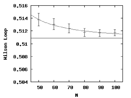
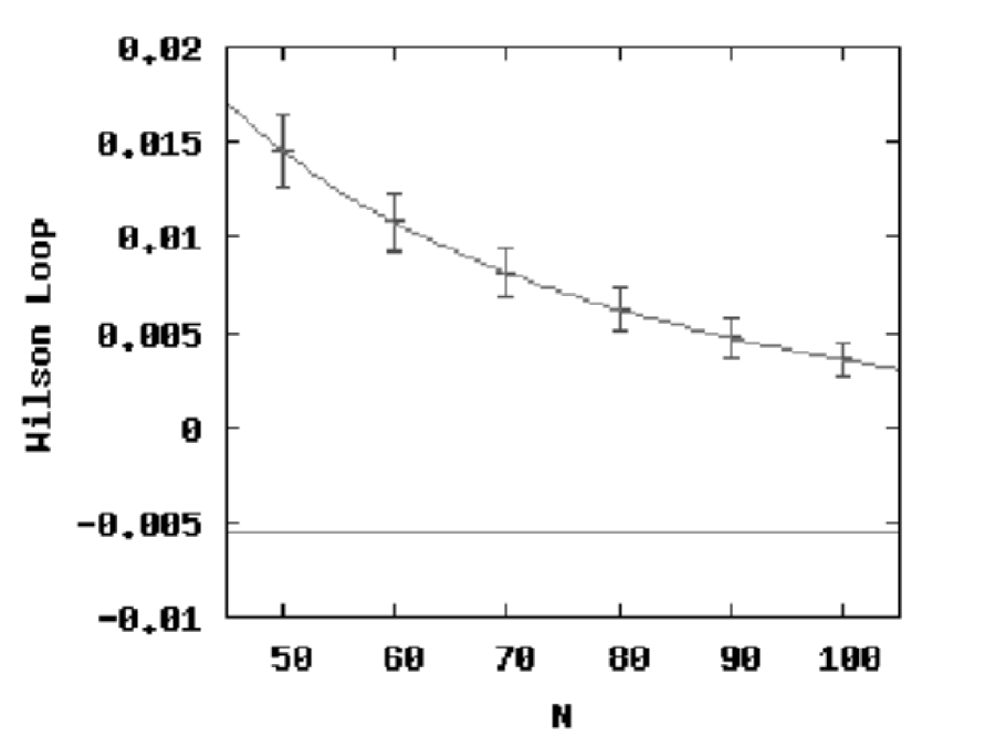
For $N=100$, only the loops satisfying $mn<10$ seem to converge (see Figs. 4 and 4). For this reason, we use only such values to extract the string tension and the string susceptibility.

Figure 3: $W[1,1]$ for $\alpha=3.73,\ \beta=0.4$. The horizontal line represents the estimated value in the large-$N$ limit, obtained by fitting the form $W[1,1]=c_{1}+c_{2}N^{c_{3}}$, where $c_{1},c_{2}$ and $c_{3}$ are constants. We find good convergence at $N=100$.

Figure 4: $W[5,5]$ for $\alpha=3.73,\ \beta=0.4$. The horizontal line represents the estimated value in the large-$N$ limit, obtained by fitting the form $W[5,5]=c_{1}+c_{2}N^{c_{3}}$, where $c_{1},c_{2}$ and $c_{3}$ are constants. We cannot find good convergence at this level.

3.2.1 $\alpha=0$: Original Weingarten model

For $\alpha=0$, it is known that [15, 6]

$$b=-1.5.\qquad(\mbox{theoretical})$$ (31)

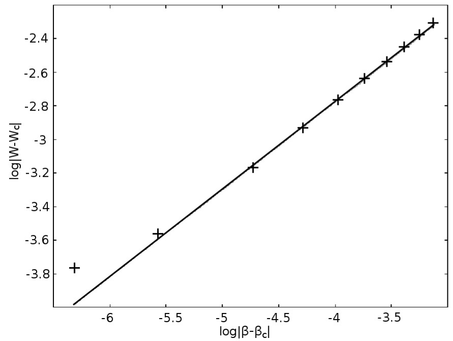
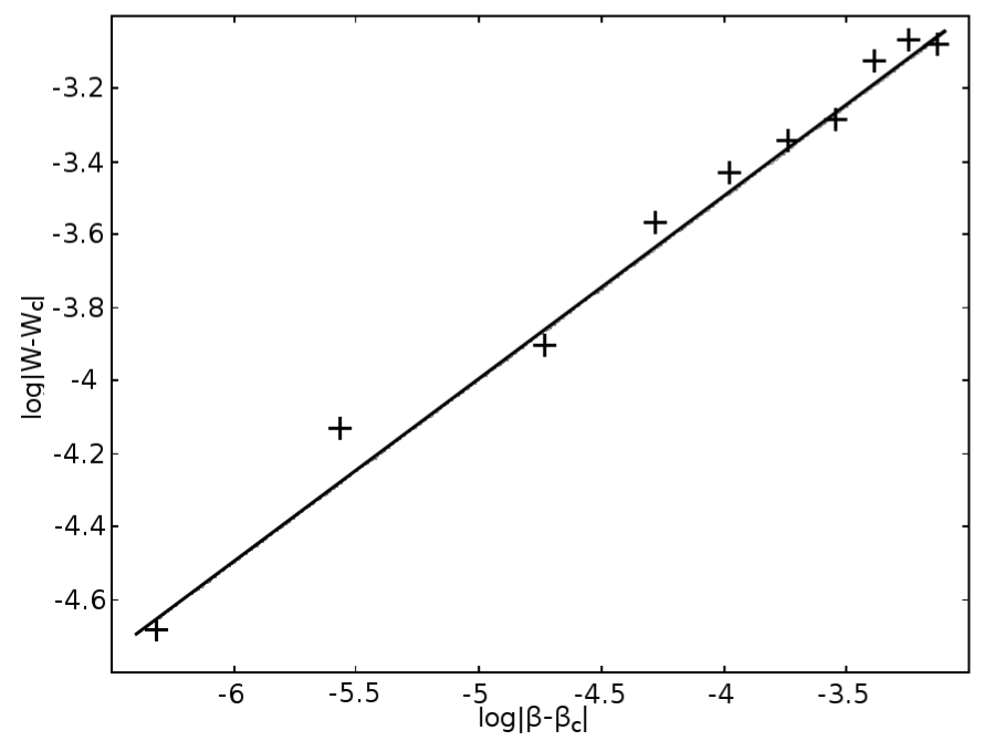
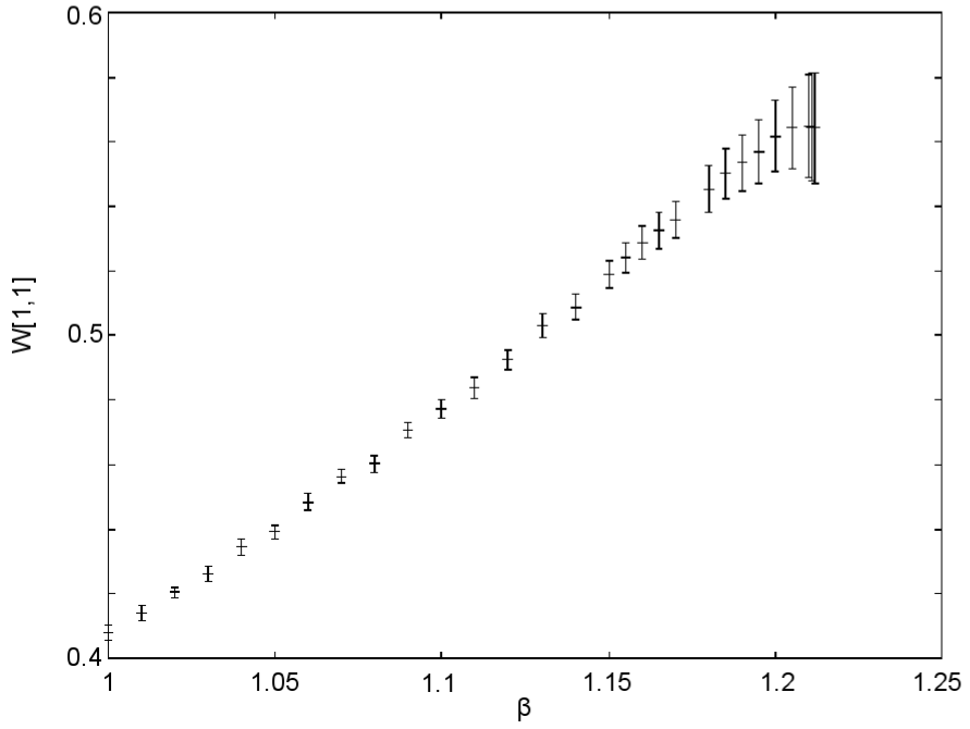
Then, taking the perimeter effect into account, we find that the numerical data are consistent with this value (Fig. 5). From the value of $W[1,1]$, we obtained

$$b=-1.50\pm 0.02.\qquad(\mbox{numerical})$$ (32)

Figure 5: $\log|W_{c}[m,n]-W[m,n]|$ as a function of $\log|\beta-\beta_{c}|$ for $\alpha=0$ (original Weingarten model), with $N=100$. Here, the perimeter effect is taken into account. The slope of the line is $0.5$. [Left] $(m,n)=(1,1)$. [Right] $(m,n)=(2,1)$.

3.2.2 $0<\alpha\lesssim 1.2$

String tension
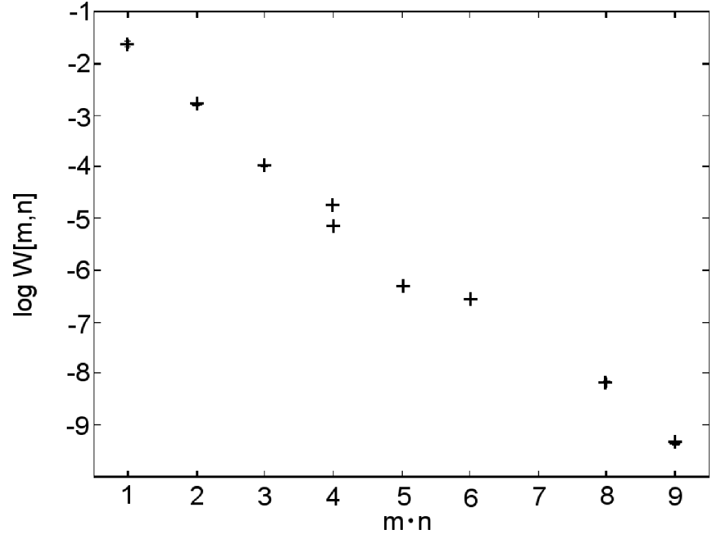
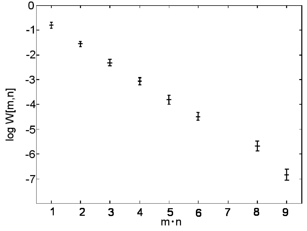
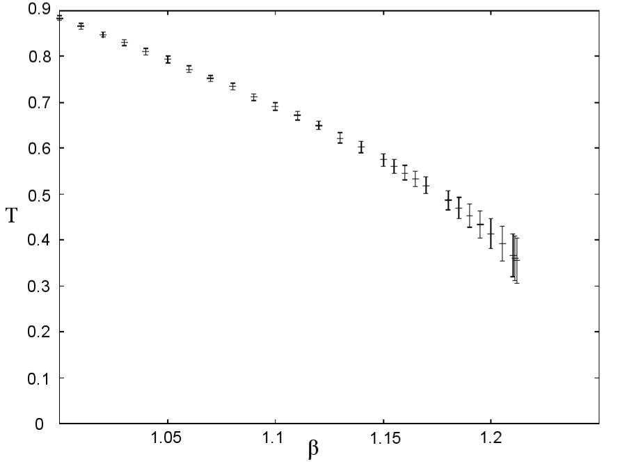
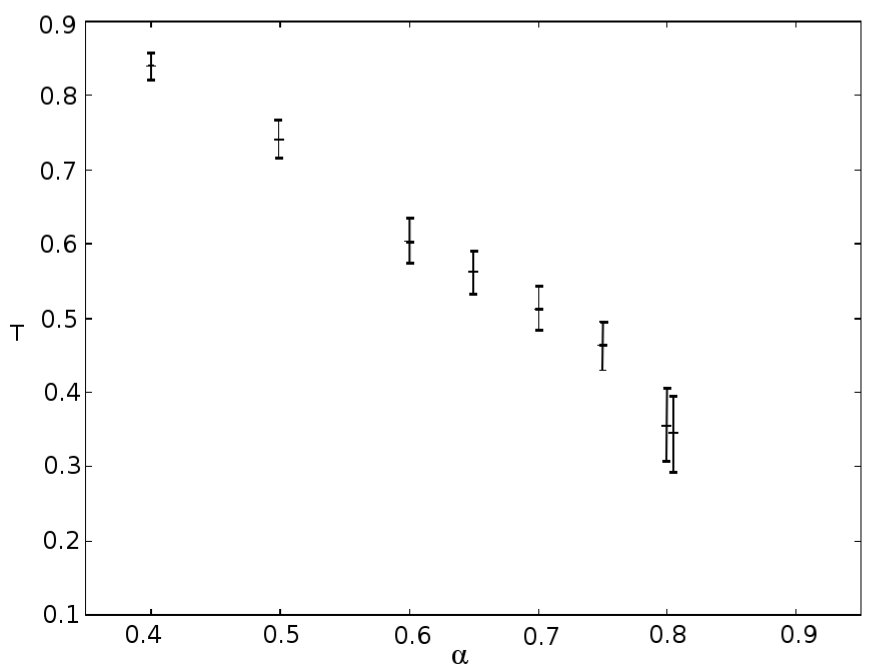
Taking the perimeter effect into account, we can determine the string tension $T$ (see Fig. 6). For fixed $\alpha$, the string tension $T$ decreases as $\beta\to\beta_{c}(\alpha)$ (Fig. 8). Although the value $T\left(\alpha,\beta_{c}(\alpha)\right)$ decreases as $\alpha$ becomes large, it remains positive (see Fig. 8).

Figure 6: $\log W[m,n]$ as a function of the $A=mn$ for $\alpha=1,N=100$. [Left] Without the perimeter effect taken into consideration. [Right] With the perimeter effect taken into consideration. The slope corresponds to $-T$. The error bars become larger due to ambiguity in $p$.

Figure 7: The string tension $T$ for $\alpha=1.2,N=100$.

Figure 8: The string tension $T$ for $\beta=\beta_{c}(\alpha),N=100$ as a function of $\alpha$.

String susceptibility
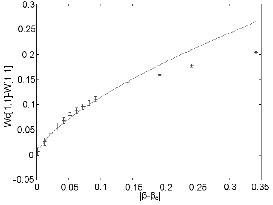
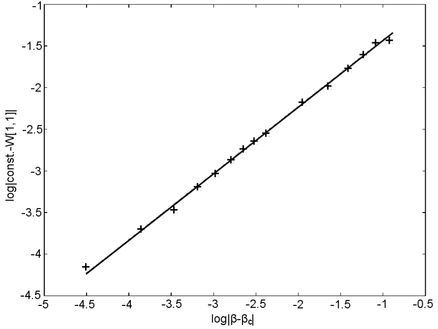
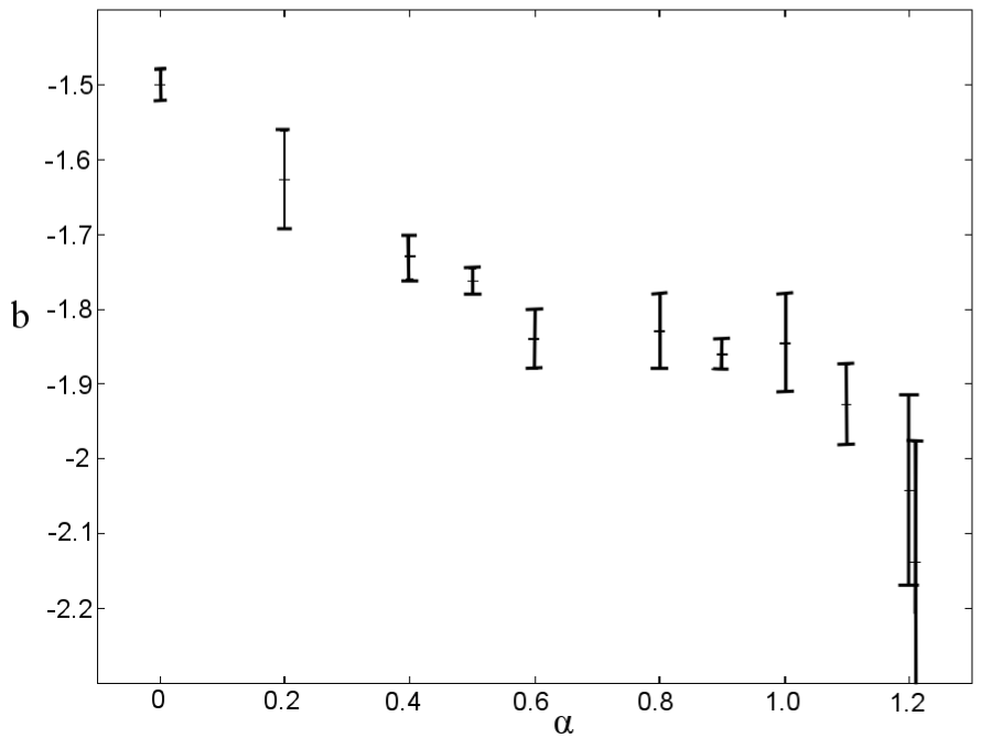
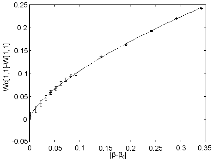
We next determine the “string susceptibility” $b(\alpha)$ using the numerical data and the expression (30). As can be seen from Fig. 9, the ansatz (30) agrees better with the data than the ansatz (25). Figure 11 displays a plot of $\log|W_{c}[1,1]-W[1,1]|$ as a function of $\log|\beta-\beta_{c}|$ for $\alpha=1$. We can read off the value $-b-1$ from the slope of the fitting line. The value of $b(\alpha)$ is plotted in Fig. 12. For $\alpha\sim 1.2$, $b(\alpha)$ seems to approach $-2$ (Fig. 12). The uncertainties here are rather large, and they come mainly from an ambiguity in the perimeter effect $p$. One of the reasons that they are so large is that the deviation of the value of the Wilson loop (at $N=100$) from that in the large-$N$ limit is not uniform but depends on the size of the loop and the parameters $\alpha$ and $\beta$. If we can use larger matrix size $N$, we would be able to make the uncertainties smaller.

Figure 9: $W_{c}[1,1]-W[1,1]$ is as a function of $\beta_{c}-\beta$ for $\alpha=1,N=100$. The curves represent the fitted form $W=W_{c}-\mbox{const}\cdot|\beta-\beta_{c}|^{-b-1}$. [Left] With the perimeter effect taken into consideration. [Right] Without the perimeter effect taken into consideration.

Figure 10: $\log|W_{c}[1,1]-W[1,1]|$ as a function of $\log|\beta-\beta_{c}|$ for $\alpha=1,N=100$. Here, the perimeter effect is taken into consideration. The line represents the fitted form, whose slope is $-b-1$.

Figure 11: $W[1,1]$ as a function of $\beta$ for $\alpha=1.2,N=100$. Here, the perimeter effect is taken into account.

Figure 12: String susceptibility $b$ as a function of $\alpha$. The result, $b=-1.50\pm 0.02$ at $\alpha=0$, is consistent with the result found in Refs. DFJ84, and KO.

3.2.3 $1.2\lesssim\alpha<\infty$

In this parametric region, a phase transition takes place at $\beta=\beta_{\mathrm{breakdown}}<\beta_{c}$. As remarked in § 3.1, the $U(1)^{2}$ symmetry seems to be broken for $\beta>\beta_{\mathrm{breakdown}}$. Therefore, it is plausible that the reduced model deviates from that on a lattice, and thus the lattice-string interpretation is not possible.

4 Conclusions and discussions

In this paper, we have reported the results of a a numerical study of the two-dimensional generalized Weingarten model (1). If we assume the relations (22) and (30), then the numerical data show that the string susceptibility approaches $-2$ as we increase the value of the parameter $\alpha$ to $\sim 1.2$. This result suggests that branched-polymer configurations are suppressed in this parametric region. We also found that the string tension decreases. However, we encountered a phase transition before the string tension becomes zero. Therefore, we cannot take the continuum limit in the reduced model studied in this paper.

There are several pontential directions for future studies. First, it is necessary to understand the present model in terms of the random surface and explain why the assumption (22) seems to be consistent with the numerical data. Doing so, we would be able to clarify whether or not our numerical result actually indicates that the branched polymer configurations are suppressed. In addition, such an understanding would be helpful for finding better models. Second, it would be interesting to study the model defined on a lattice [1]. In the case of the large-$N$ reduced $d$-dimensional $U(N)$ gauge theory ($d\geq 3$), the breakdown of $U(1)^{d}$ is an artifact of the reduced model; if the model is defined on a lattice of size $L^{d}$, then the $U(1)^{d}$ symmetry is not broken to the weaker coupling as $L$ increases [11]. If similar phenomena exist in the present case, then using the model with $L>1$, we could study the larger parametric region, and we may be able to find a point at which we can take the continuum limit. Third, we can also consider higher-dimensional models. In this case, the lattice-string interpretation may be valid in the parametric region in which some of the $U(1)$s remain unbroken. This point is worth studying. We hope to report analysis of these models in future publications.

Appendix A Comparison with the Two-Dimensional Generalized Weingarten Model without a Twist

A.1 Two-dimensional generalized Weingarten model without a twist

Figure 13: Phase diagram of the two-dimensional generalized Weingarten model without a twist for $\alpha\lesssim 1$.

Figure 14: Phase diagram of the two-dimensional generalized Weingarten model without a twist for $\alpha\gtrsim 1$. (This figure is based on Fig. 10 of Ref. HKKK.)

In this section, we consider the original, untwisted generalized Weingarten model in two dimensions.

For large, fixed $\alpha$ there are two curves of first-order phase transitions. We call them $\beta_{1}$ and $\beta_{2}$ in ascending order. They correspond to the breakdown of the $U(1)^{2}$ symmetry. If we increase $\beta$ with $\alpha$ fixed, $U(1)^{2}$ is broken to $U(1)$ at $\beta_{1}$, and then it is broken completely at $\beta_{2}$. The values of $\beta_{1}$ and $\beta_{2}$ seem to diverge as $\alpha^{-1}\to 0$. This is consistent with the analytic result, in which $U(1)^{2}$ is not broken. At small $\alpha$, $\beta_{1}$ and $\beta_{2}$ seem to become equal. This transition persists to $\alpha\sim 1.2$ where it merges with the boundary of the metastable parametric region. Near the boundary of the well-defined region $\beta<\alpha$, the $U(1)^{2}$ symmetry is restored. In Fig. 14, this line of restoration of $U(1)^{2}$ is drawn by a dotted line near $\alpha\sim 1.2$, because the restoration cannot be seen clearly in this region.

In the parametric region where the $U(1)^{2}$ symmetry is not broken, our reduced model is equivalent to the model defined on a lattice [1] through the large-$N$ reduction. If this symmetry is broken, then the reduced model deviates from that on a lattice, and the lattice-string interpretation is not valid .

A.2 Comparison of untwisted and twisted models

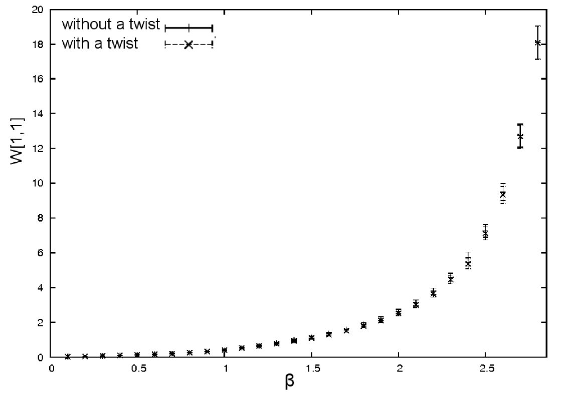
Figure 15: Plot of the expectation value of $1\times 1$ Wilson loop for $\alpha^{-1}=0.3,N=50$.

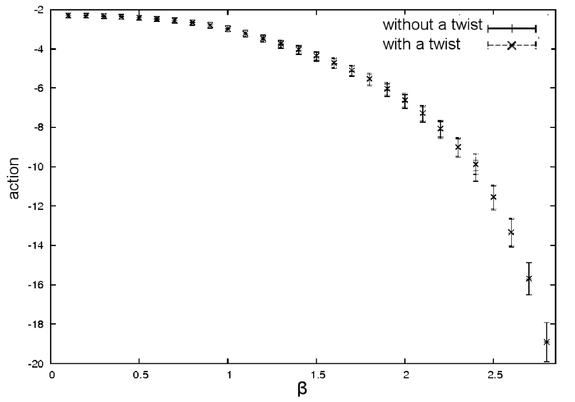
Figure 16: Plot of the expectation value of the action for $\alpha^{-1}=0.3,N=50$.

In this subsection, in order to avoid confusion, we indicate the physical quantities in the twisted model with the subscript $T$. For example, Wilson loops are denoted as

$$W[m,n](\alpha,\beta),\quad\quad(\mbox{without twist})$$ (33)

$$W_{T}[m,n](\alpha,\beta)=(-)^{mn}W[m,n](\alpha,-\beta).\quad\quad(\mbox{with maximal twist})$$ (34)

Here we have included the phase $(-)^{mn}$ so that the two prescriptions give the same value in the strong coupling region:

$$W[m,n](\alpha,\beta)=W_{T}[m,n](\alpha,\beta).\qquad(\mbox{strong coupling})$$ (35)

In Fig. 16, we plot the expectation values of $1\times 1$ Wilson loops for $\alpha^{-1}=0.3$. We see that $W[1,1]$ and $W_{T}[1,1]$ indeed take the same value. We can also see that the expectation values of the action are nearly equal (Fig. 16).

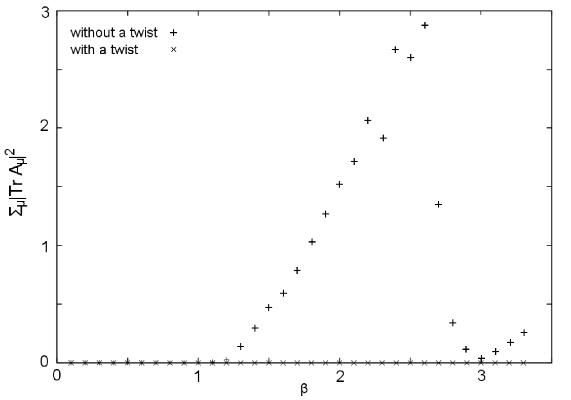
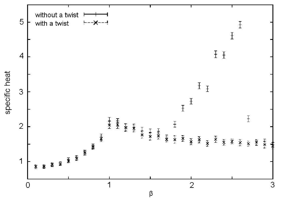
It is interesting that the two prescriptions seem to give the same expectation values for the Wilson loops not only in the strong coupling region but also in the weak coupling region, which is separated from the strong coupling region by a phase transition; indeed, as can be seen from Fig. 18, phase transitions take place naer $\beta_{1}(\alpha^{-1}=0.3)=1$ both in the twisted and untwisted models. In the case of the untwisted model, this transition corresponds to the breakdown of $U(1)^{2}$ (see Fig. 18). In the case of the twisted model, because the expectation value of $\sum_{\mu}|\mathrm{Tr}A_{\mu}|$ remains nearly equal to zero, this transition does not correspond to the complete breakdown of one of the $U(1)$s; it may represent a breakdown to ${\mathbb{Z}}_{n}$ for some integer $n$.

Figure 17: Plot of the specific heat for $\alpha^{-1}=0.3,N=50$.

Figure 18: Plot of the expectation value of $\sum_{\mu}|\mathrm{Tr}A_{\mu}|^{2}$ for $\alpha^{-1}=0.3,N=50$.

References

• [1] E-M. Ilgenfritz, Y.ย M. Makeenko and T.ย V. Shakhbazian, \PLB172,1986,81.
• [2] M.ย Hanada, T.ย Kanai, H.ย Kawai and F.ย Kubo, \PTP115,2006,1167.
• [3] T. Eguchi and H. Kawai, \PLB114,1982,247.
• [4] T. Eguchi and H. Kawai, \PRL48,1982,1063.
• [5] D. Weingarten, \PLB90,1980,280.
• [6] H. Kawai and Y. Okamoto, \PLB130,1983,415.
• [7] H. Kawai, Nucl. Phys. B (Proc. Suppl.) 26 (1992), 93.
• [8] T. Takayanagi and N. Toumbas, \JHEP0307,2003,064.
M. R. Douglas, I. R. Klebanov, D. Kutasov, J. Maldacena, E. Martinec and N. Seiberg, in From fields to strings, vol. 3:1758, M. Shifman, (ed.) et al; hep-th/0307195.
• [9] G. Paffuti and P. Rossi, \PLB92,1980,321.
• [10] D. J. Gross and E. Witten, \PRD21,1980,446.
• [11] R. Narayanan and H. Neuberger, \PRL91,2003,081601.
J. Kiskis, R. Narayanan and H. Neuberger, \PLB574,2003,65.
• [12] T. Hotta, J. Nishimura and A. Tsuchiya, \NPB545,1999,543.
• [13] T.ย Eguchi and H.ย Kawai, \PLB110,1982,143.
• [14] B.ย Durhuus, J.ย Frohlich and T.ย Jonsson, \NPB225,1983,185.
• [15] B.ย Durhuus, J.ย Frohlich and T.ย Jonsson, \NPB240,1984,453.
• [16] A.ย Gonzalez-Arroyo and M.ย Okawa, \PRD27,1983,2397.
• [17] A.ย Gonzalez-Arroyo, R.ย Narayanan and H.ย Neuberger, \PLB631,2005,133.