Abstract

As the Hubbard energy at half filling is believed to reproduce at strong coupling (part of) the all loop expansion of the dimensions in the $SU(2)$ sector of the planar ${\cal N}=4$ SYM, we compute an exact non-perturbative expression for it. For this aim, we use the effective and well-known idea in 2D statistical field theory to convert the Bethe Ansatz equations into two coupled non-linear integral equations (NLIEs). We focus our attention on the highest anomalous dimension for fixed bare dimension or length, $L$, analysing the many advantages of this method for extracting exact behaviours varying the length and the ’t Hooft coupling, $\lambda$. For instance, we will show that the large $L$ (asymptotic) expansion is exactly reproduced by its analogue in the BDS Bethe Ansatz, though the exact expression clearly differs from the BDS one (by non-analytic terms). Performing the limits on $L$ and $\lambda$ in different orders is also under strict control. Eventually, the precision of numerical integration of the NLIEs is as much impressive as in other easier-looking theories.

Keywords: Quantum Integrability (Bethe Ansatz); Non-Linear Integral Equation; Hubbard model; Super Yang-Mills theories.

1 Prologue

It is a modern achievement that gauge theories and in particular supersymmetric gauge theories hide many realisations of the algebraic geometry theorisation (cf. [1] just as a recent monumental reference on the last discovered parallel and many other features).

More in specific, the AdS/CFT correspondence [2] should be a general dictionary, which would equate – among other physical objects – energies of string states to anomalous dimensions of local gauge-invariant operators of a dual conformal quantum field theory. Proving or even testing this duality in full generality may be a formidable task, but the integrability properties of the ${\cal N}=4$ super Yang-Mills (SYM) theory have proved to be extremely useful to understand how it may work and to which extent.

The identification [3] of the one-loop dilatation operator of scalar gauge-invariant fields with bare dimension $L$ with an $SO(6)$ integrable chain with $L$ sites, reducing in the $SU(2)$ subspace to the spin $1/2$-XXX Heisenberg chain, allowed, by using the Bethe Ansatz technique [4], to test the one-loop AdS/CFT duality in many cases [5, 6, 7] beyond the BMN conditions [8]. In the aforementioned cases, special emphasis has been delivered to the $1/L$ correction, as this would result as the first quantum correction in string theory; and more generally all the finite size $L$ corrections would have a similar stringy origin and importance. Soon afterwards, integrability of ${\cal N}=4$ SYM at higher loops started to be hinted and hunted [9]. After various attempts and tests (cf. for instance [10]), eventually in [11] an all loop asymptotic expression has been proposed for the eigenvalues of the dilatation operator in the $SU(2)$ sub-sector, in terms of the solutions of Bethe Ansatz-like equations, derived by assuming BMN scaling and perturbative integrability. Moreover, this proposal (named after them BDS equations) was shown to give the correct (truncated) Bethe equations for the five loop dilatation operator, after deriving the latter as an operator. Nevertheless, the BDS equations are valid only asymptotically, that is for fixed $L$ when the ’t Hooft coupling $\lambda$ is small enough that the ${\cal O}(\lambda^{L})$ term ($L$ loops) may be neglected along with the higher order powers. In fact, the higher loops are clearly affected by the chain wrapping problem – namely an interaction range longer than the chain length – which is not taken into account by the BDS proposal. In this respect, an important progress was the remark, by Rej, Serban and Staudacher [12], that the $SU(2)$ dilatation operator could be reproduced up to three loops by the strong coupling expansion of the Hamiltonian of the half-filled Hubbard model. Many tests of the proposal [12] started to be performed (cf. for instance [13]), while it seems now clear that starting from four loops the Hubbard model will reproduce only part of the entire contributions (likely the ’rational ones’), the string theory/gauge theory discrepancies motivating the introduction of a specific dressing factor [14] also in gauge theory. Indeed, although the dressing factor would also care for the large $\lambda$ behaviour, it is unclear for now how to insert it into the two Lieb-Wu Bethe equations for the Hubbard model [15]. On the contrary, it is manifest its introduction into the BDS Bethe Ansatz, and therefore a comparative study of BDS versus Hubbard model is one of the motivations of this paper.

In a previous paper [16] we proposed a description of the highest and immediately lower energy states, for both the $SO(6)$ chain and the BDS model, based on the non-linear integral equation (NLIE). The NLIE was first introduced in [17, 18, 19] for studying the finite size scaling of the ground state and of the excited states in (critical and off-critical) statistical (lattice) field theories respectively. Although it is equivalent to the set of all the Bethe Ansatz equations, it is often more suitable for numerical and analytical calculations, especially when it is important, like in the present case, to detect how the anomalous dimension (energy) behaves with the length $L$ (especially in large $L$ investigations). In fact, it condensates into a single (or only very few) integral equation(s) many algebraic equations. In this respect, we will prove here that it is a right tool to deal with the two possible ordering of the limits of large size $L$ and large coupling $\lambda$. Furthermore, we will find a systematic way to perform the two expansions for small coupling and large coupling at any fixed size.

In this paper we want to introduce the NLIEs as a profitable treatment of the Hubbard model, especially for the understanding of the exact scaling behaviour of the dimension (energy) with $\lambda$ and $L$. We will concentrate on the highest energy (anomalous dimension) state of the half-filled Hubbard model ($SU(2)$ sub-sector of ${\cal N}=4$ SYM). This state is described by two coupled NLIEs which will be written in Section 3. In Section 4 we will give an exact expression for its energy, as a function of the coupling $g$ and the length of the chain $L$, in terms of the solution of the two coupled NLIEs. This peculiar expression for the energy allows a comparison at large length $L$ (Section 5) with the analogous result coming from the BDS chain: we will show that the $1/L$ leading term and all the next finite size corrections (power-like and logarithmic) in fact coincide (i.e. the usual large $L$ asymptotic expansion do coincide), the difference being captured by exponentially small corrections (whose leading contribution we estimated at strong coupling). Moreover, as a consistency check of our findings, in Section 6 the weak and strong coupling limits of the NLIEs on one hand and of the energy on the other hand will be studied and shown to reproduce the known results. The strong coupling for the BDS model is also carefully analysed. As a consequence, Section 7 is devoted to the understanding of the ordering of the two distinct limits $\lambda\rightarrow+\infty$ and $L\rightarrow+\infty$, both in the Hubbard and BDS models. Eventually, a detailed numerical analysis is carried out in the last Section 8.

2 The Hubbard model: a bird’s-eye view

The Hubbard model was introduced as a simplified model for strongly correlated electrons on a lattice [20]. In one dimension, it describes $N_{\text{e}}$ electrons moving on a chain with $L$ sites and interacting via the Hamiltonian

$$H=-t\sum_{i=1}^{L}\sum_{\sigma=\uparrow,\downarrow}\left(c_{i,\sigma}^{\dagger}c_{i+1,\sigma}+c_{i+1,\sigma}^{\dagger}c_{i,\sigma}\right)+U\sum_{i=1}^{L}c_{i,\uparrow}^{\dagger}c_{i,\uparrow}c_{i,\downarrow}^{\dagger}c_{i,\downarrow}\,,$$ (2.1)

where $c_{i,\sigma}^{\dagger}$, $c_{i,\sigma}$ are (fermionic) canonical creation and annihilation operators respectively, $t$ is the strength of the kinetic nearest-neighbour hopping term, $U$ the coupling constant of the density potential and, for our interests, periodic boundary conditions are assumed, i.e. $c_{i+L,\sigma}=c_{i,\sigma}$, $c_{i+L,\sigma}^{\dagger}=c_{i,\sigma}^{\dagger}$.

In the relevant paper [12], a precise sub-set of the energies $E$ of (2.1) was conjectured to be proportional to the anomalous contribution $\gamma$ to the conformal dimensions in the $SU(2)$ scalar sector of ${\cal N}=4$ super Yang-Mills theory in the planar limit,

$$\gamma=\frac{\lambda}{8\pi^{2}}E\,,$$ (2.2)

provided we restrict ourselves to the half-filling case $N_{\text{e}}=L$ and also equate the length $L$ to the number of constituent operators.

Now, a very important part of the correspondence between an integrable system and a gauge theory is the mapping of the coupling constants, and the latter can be easily argued to be a strong-weak coupling duality for many reasons. Therefore, one possible choice, reproducing the known results up to three loops, may well be [12]

$$t=-\frac{1}{{\sqrt{2}}g}=-\frac{2\pi}{\sqrt{\lambda}}\,,\quad U=-\frac{1}{g^{2}}=-\frac{8\pi^{2}}{\lambda}\,,$$ (2.3)

where $\lambda=Ng_{YM}^{2}=8\pi^{2}g^{2}$ is the ’t Hooft coupling of the $SU(N)$ SYM theory in the planar limit ($N\rightarrow\infty$). But this can be modified by higher order contributions still preserving, of course, the matching outcomes. Actually, to have a loop expansion of (2.2) in $g^{2}$ with the right wrapping phenomenon occurring at ${\cal O}(g^{2L})$, we need to introduce a constant magnetic flux $\phi$ [12],

$$H=\frac{1}{{\sqrt{2}}g}\sum_{i=1}^{L}\sum_{\sigma=\uparrow,\downarrow}\left(e^{i\phi}c_{i,\sigma}^{\dagger}c_{i+1,\sigma}+e^{-i\phi}c_{i+1,\sigma}^{\dagger}c_{i,\sigma}\right)-\frac{1}{g^{2}}\sum_{i=1}^{L}c_{i,\uparrow}^{\dagger}c_{i,\uparrow}c_{i,\downarrow}^{\dagger}c_{i,\downarrow}\,,$$ (2.4)

distinguishing odd and even lengths: $\phi=0$ when $L$ is odd and $\phi=\frac{\pi}{2L}$ when $L$ is even.

The Hubbard hamiltonian (2.1) describes an integrable model (infinite many conserved charges in involution), which was diagonalised by Lieb and Wu by Bethe Ansatz in 1968 [15]. The twisted Hamiltonian (2.4) is still integrable and the Lieb-Wu equations easily generalise. In the half-filling case they read [12]

$$e^{i\hat{k}_{j}L} = \prod_{l=1}^{M}\frac{u_{l}-\frac{2t}{U}\sin(\hat{k}_{j}+\phi)-\frac{i}{2}}{u_{l}-\frac{2t}{U}\sin(\hat{k}_{j}+\phi)+\frac{i}{2}}$$

$$\prod_{j=1}^{L}\frac{u_{l}-\frac{2t}{U}\sin(\hat{k}_{j}+\phi)+\frac{i}{2}}{u_{l}-\frac{2t}{U}\sin(\hat{k}_{j}+\phi)-\frac{i}{2}} = \mathop{\prod_{m=1}}_{m\not=l}^{M}\frac{u_{l}-u_{m}+i}{u_{l}-u_{m}-i}\,,$$ (2.5)

where $M$ is the number of down spins. The spectrum of the Hamiltonian is then given in terms of the pseudo-momenta $\hat{k}_{j}$, by the free dispersion relation

$$E=-2t\sum_{j=1}^{L}\cos(\hat{k}_{j}+\phi)\,.$$ (2.6)

Starting from here, we will equivalently derive two coupled nonlinear integral equations (NLIEs) for the antiferromagnetic state of the model at any value of $L$, thanks to the methods used in [16]. For reason of completeness, we point out that the thermodynamics (infinite length $L$, but finite temperature) of the Hubbard model has been studied [22, 23] by means of three NLIEs (for a summary of the procedure and a complete list of references see [24]). This approach was based on the equivalence of the (quantum) one-dimensional Hubbard model with the (classical) two-dimensional Shastry model. For the gauge theory understanding, we need to obtain energies of the Hubbard model at zero temperature, but at any value of the length $L$. This completely justifies our approach, and a fortiori in the perspective of extending our calculations to excited states (i.e. lower dimension operators in the SYM spectrum).

3 Two non-linear integral equations (NLIEs)

Looking at the Bethe equations (2.5), we define the function

$$\Phi(x,\xi)=i\ln\frac{i\xi+x}{i\xi-x}\,,$$ (3.1)

with the branch cut of $\ln(z)$ along the real negative $z$-axis in such a way that $-\pi<\arg z<\pi$. Then, we perform a gauge transformation which amounts to adding the magnetic flux:

$$k_{j}=\hat{k}_{j}+\phi\,.$$ (3.2)

After a possible choice of the counting functions as

$$W(k) = L(k-\phi)-\sum_{l=1}^{M}\Phi\left(u_{l}-\frac{2t}{U}\sin k,\frac{1}{2}\right)\,,$$ (3.3)

$$Z(u) = \sum_{j=1}^{L}\Phi\left(u-\frac{2t}{U}\sin k_{j},\frac{1}{2}\right)-\sum_{m=1}^{M}\Phi\left(u-u_{m},1\right)\,,$$ (3.4)

we can rewrite the Bethe equations, by taking their logarithm, in the usual form of quantisation conditions for the Bethe roots $\{k_{j},u_{l}\}$,

$$W(k_{j}) = \pi M+2\pi I^{w}_{j}\,,$$ (3.5)

$$Z(u_{l}) = \pi(M-L+1+2I^{z}_{l})\,.$$ (3.6)

From now on, we specialise our treatment to the highest energy state, consisting of the maximum number $M=L/2$ of real roots $u_{l}$ and of $L$ real roots $k_{j}$. For simplicity reasons, we restrict ourselves to the case $M\in 2{{{{N}}}}$ (the remaining case $M\in 2{{{{N}}}}+1$ is a simple modification of this case), which obviously implies $L\in 4{{{{N}}}}$.

In the definition of the counting functions (3.3, 3.4) we have to deal with sums of functions computed on real Bethe roots, $k_{j}$ and $u_{l}$. Let us first concentrate on functions of $k_{j}$. We notice that $k_{j}$ may run only within the first Brillouin zone $[-\pi,\pi)$ and that the functions of $k_{j}$ involved are periodic with period $2\pi$. On the other hand, the counting function $W(k)$ is quasi-periodic on that interval and $e^{iW(k)}$ and $W^{\prime}(k)$ are indeed periodic. Using the Cauchy theorem to circulate the interval $[-\pi,\pi)$ by a small displacement $\epsilon>0$ (this periodic case has been developed in [25]), we get

$$\sum_{j=1}^{L}f(k_{j})= - \int_{\pi}^{-\pi}\frac{dk}{2\pi i}f(k+i\epsilon)\frac{iW^{\prime}(k+i\epsilon)e^{iW(k+i\epsilon)}}{1-e^{iW(k+i\epsilon)}}-$$ (3.7)

$$- \int_{-\pi}^{\pi}\frac{dk}{2\pi i}f(k-i\epsilon)\frac{iW^{\prime}(k-i\epsilon)e^{iW(k-i\epsilon)}}{1-e^{iW(k-i\epsilon)}}\,,$$

where the two complex integrals along $-\epsilon<{\mbox{ Im}}k<\epsilon$ at ${\mbox{Re}}k=\pm\pi$ have been neglected thanks to the periodicity properties of $f(k)$ and $e^{iW(k)}$. A thumb rule to understand this logarithmic indicator formula goes as follows: since $W^{\prime}(k)>0$ , the first integral is simply the logarithmic derivative in the following formula, but the second one is not because of the non-analyticity of the logarithm . Nevertheless, the latter can be simply manipulated into a logarithmic derivative of an analytic function plus an extra piece:

$$\sum_{j=1}^{L}f(k_{j}) = -\int_{-\pi}^{\pi}\frac{dk}{2\pi i}f(k+i\epsilon)\frac{d}{dk}\ln\left[1-e^{iW(k+i\epsilon)}\right]+$$

$$+ \int_{-\pi}^{\pi}\frac{dk}{2\pi i}f(k-i\epsilon)\frac{d}{dk}\ln\left[1-e^{-iW(k-i\epsilon)}\right]+\int_{-\pi}^{\pi}\frac{dk}{2\pi}f(k-i\epsilon)W^{\prime}(k-i\epsilon)\,.$$

To make the last term useful, we can compute it along the real axis without any harm, because of the periodicity of $f(k)$ and $W^{\prime}(k)$; then, after integrating by parts the two integrals before it, we arrive at

$$\sum_{j=1}^{L}f(k_{j}) = \int_{-\pi}^{\pi}\frac{dk}{2\pi i}f^{\prime}(k+i\epsilon)\ln\left[1-e^{iW(k+i\epsilon)}\right]-$$

$$- \int_{-\pi}^{\pi}\frac{dk}{2\pi i}f^{\prime}(k-i\epsilon)\ln\left[1-e^{-iW(k-i\epsilon)}\right]+\int_{-\pi}^{\pi}\frac{dk}{2\pi}f(k)W^{\prime}(k)\,,$$

because the boundary terms vanish as a consequence of the periodicity of $f(k)$ and $e^{iW(k)}$. Upon integrating by parts the last term, we finally obtain

$$\sum_{j=1}^{L}f(k_{j}) = -\int_{-\pi}^{\pi}\frac{dk}{2\pi}f^{\prime}(k)W(k)+{\mbox{ Im}}\int_{-\pi}^{\pi}\frac{dk}{\pi}f^{\prime}(k+i\epsilon)\ln\left[1-e^{iW(k+i\epsilon)}\right]+$$ (3.10)

$$+ \left[\frac{f(k)W(k)}{2\pi}\right]^{\pi}_{-\pi}\,.$$

We will mainly use such formula in the $\epsilon\rightarrow 0^{+}$ limit,

$$\sum_{j=1}^{L}f(k_{j})=-\int_{-\pi}^{\pi}\frac{dk}{2\pi}f^{\prime}(k)W(k)+\int_{-\pi}^{\pi}\frac{dk}{\pi}f^{\prime}(k){\mbox{ Im}}\ln\left[1-e^{iW(k+i0)}\right]+\left[\frac{f(k)W(k)}{2\pi}\right]^{\pi}_{-\pi}\,,$$ (3.11)

which reads as (3.11) because of the supposed analyticity of $f(k)$ on the real axis.

For what concerns a sum of a generic function $g(x)$ for $x$ being any root $u_{l}$ (which is in principle everywhere in the real axis for the ground state), we can go along similar steps and repeat the original procedure for $x\in\mathbb{R}$ [18, 19]. In this case the boundary terms appearing during the computations can be neglected thanks to different applicable reasons. One sufficient set of conditions, which apply to the case $g=\Phi$, relevant for the derivations of the NLIEs for $W$ and $Z$, turns out to be

$$Z^{\prime}(\pm\infty+iy)=0\,,\,-\epsilon<y<\epsilon\,;\quad g(+\infty)=-g(-\infty)\,,\quad Z(+\infty)=-Z(-\infty)\,,$$

$$\quad Z(+\infty\pm i\epsilon)=-Z(-\infty\mp i\epsilon)\,,\quad g(+\infty\pm i\epsilon)=-g(-\infty\mp i\epsilon).$$ (3.12)

In formulæ  we can write

$$\sum_{l=1}^{M}g(u_{l})=-\int_{-\infty}^{\infty}\frac{dx}{2\pi}g^{\prime}(x)Z(x)+{\mbox{ Im}}\int_{-\infty}^{\infty}\frac{dx}{\pi}g^{\prime}(x+i\epsilon)\ln\left[1+e^{iZ(x+i\epsilon)}\right]\,,$$ (3.13)

or, in the $\epsilon\rightarrow 0^{+}$ limit,

$$\sum_{l=1}^{M}g(u_{l})=-\int_{-\infty}^{\infty}\frac{dx}{2\pi}g^{\prime}(x)Z(x)+\int_{-\infty}^{\infty}\frac{dx}{\pi}g^{\prime}(x){\mbox{ Im}}\ln\left[1+e^{iZ(x+i0)}\right]\,.$$ (3.14)

Eventually, we have our building blocks in formulæ  (3.11) and (3.14), where the r.h.s. is written through each counting function respectively. Let us apply them to the definition of the $W(k)$,

$$W(k) = L(k-\phi)+\int_{-\infty}^{\infty}\frac{dx}{2\pi}\Phi^{\prime}\left(x-\frac{2t}{U}\sin k,\frac{1}{2}\right)Z(x)-$$ (3.15)

$$- \int_{-\infty}^{\infty}\frac{dx}{\pi}\Phi^{\prime}\left(x-\frac{2t}{U}\sin k,\frac{1}{2}\right){\mbox{Im}}\ln\left[1+e^{iZ(x+i0)}\right]\,,$$

and to the definition of $Z(u)$,

$$Z(u) = L\Phi\left(u,\frac{1}{2}\right)+\frac{2t}{U}\int_{-\pi}^{\pi}\frac{dk}{2\pi}\Phi^{\prime}\left(u-\frac{2t}{U}\sin k,\frac{1}{2}\right)\cos k\>W(k)-$$

$$- \frac{2t}{U}\int_{-\pi}^{\pi}\frac{dk}{\pi}\Phi^{\prime}\left(u-\frac{2t}{U}\sin k,\frac{1}{2}\right)\cos k{\mbox{ Im}}\ln\left[1-e^{iW(k+i0)}\right]-$$

$$- \int_{-\infty}^{\infty}\frac{dy}{2\pi}\Phi^{\prime}(u-y,1)Z(y)+\int_{-\infty}^{\infty}\frac{dy}{\pi}\Phi^{\prime}(u-y,1){\mbox{ Im}}\ln\left[1+e^{iZ(y+i0)}\right]\,.$$

Inserting in the equation for $Z$ the expression for $W$ coming from (3.15), we get

$$Z(u) = L\Phi\left(u,\frac{1}{2}\right)+L\frac{2t}{U}\int_{-\pi}^{\pi}\frac{dk}{2\pi}\Phi^{\prime}\left(u-\frac{2t}{U}\sin k,\frac{1}{2}\right)\cos k\>(k-\phi)-$$ (3.17)

$$- \int_{-\infty}^{\infty}\frac{dy}{2\pi}\Phi^{\prime}(u-y,1)\,Z(y)+\int_{-\infty}^{\infty}\frac{dy}{\pi}\Phi^{\prime}(u-y,1){\mbox{ Im}}\ln\left[1+e^{iZ(y+i0)}\right]-$$

$$- \frac{2t}{U}\int_{-\pi}^{\pi}\frac{dk}{\pi}\Phi^{\prime}\left(u-\frac{2t}{U}\sin k,\frac{1}{2}\right)\cos k{\mbox{ Im}}\ln\left[1-e^{iW(k+i0)}\right]\,,$$

where we used the following cancellation of terms,

$$\int_{-\pi}^{\pi}dk~{}\Phi^{\prime}\left(x-\frac{2t}{U}\sin k,\frac{1}{2}\right)\cos k~{}\Phi^{\prime}\left(y-\frac{2t}{U}\sin k,\frac{1}{2}\right)=0\,,$$ (3.18)

which can be easily proven by performing the change of variable $k\rightarrow\pi-k$. We now write the equation for $Z(u)$ (3.17) in terms of Fourier transforms, using

$$\hat{\Phi}(p,\xi)=\frac{2\pi}{i}P\left(\frac{1}{p}\right)e^{-\xi|p|}\,,$$ (3.20)

where $P$ indicates the principal value distribution. We obtain the following expression,

$$\hat{Z}(p) = L2\pi\frac{e^{-\frac{|p|}{2}}}{i}P\left(\frac{1}{p}\right)+L\frac{2t}{U}\int_{-\pi}^{\pi}dk\ e^{-i\frac{2tp}{U}\sin k}e^{-\frac{|p|}{2}}\cos k~{}(k-\phi)-$$ (3.21)

$$- e^{-|p|}\hat{Z}(p)+2e^{-|p|}\hat{L}_{Z}(p)-\frac{4t}{U}e^{-\frac{|p|}{2}}\int_{-\pi}^{\pi}dk\ e^{-i\frac{2tp}{U}\sin k}\cos k~{}L_{W}(k)=$$

$$= L\frac{2\pi}{i}P\left(\frac{1}{p}\right)e^{-\frac{|p|}{2}}J_{0}\left(\frac{2tp}{U}\right)-e^{-|p|}\hat{Z}(p)+2e^{-|p|}\hat{L}_{Z}(p)-$$

$$- \frac{4t}{U}e^{-\frac{|p|}{2}}\int_{-\pi}^{\pi}dk\,e^{-i\frac{2tp}{U}\sin k}\cos k~{}L_{W}(k)\,,$$

where we used the integral definition of the Bessel function $J_{0}(z)$,

$$J_{0}(z)=\int_{-\pi}^{\pi}\frac{dk}{2\pi}\,e^{i\,z\sin k}\,,$$ (3.22)

and also the following shorthand notations

$$L_{W}(k)={\mbox{Im}}\ln\left[1-e^{iW(k+i0)}\right]\,,\quad L_{Z}(x)={\mbox{Im}}\ln\left[1+e^{iZ(x+i0)}\right]\,.$$ (3.23)

The terms proportional to $\hat{Z}(p)$ are now collected and reorganized as

$$\hat{Z}(p)=L\frac{\pi}{i}P\left(\frac{1}{p}\right)\frac{J_{0}\left(\frac{2tp}{U}\right)}{\cosh\frac{p}{2}}+\frac{2}{1+e^{|p|}}\hat{L}_{Z}(p)-\frac{2t}{U}\frac{1}{\cosh\frac{p}{2}}\int_{-\pi}^{\pi}dk~{}e^{-i\frac{2tp}{U}\sin k}\cos k\>L_{W}(k)\,,$$

and, coming back to the ’coordinate’ space, we obtain the first of two nonlinear integral equations for our counting functions,

$$Z(u) = L\int_{-\infty}^{\infty}\frac{dp}{2p}\sin(pu)\frac{J_{0}\left(\frac{2tp}{U}\right)}{\cosh\frac{p}{2}}+2\int_{-\infty}^{\infty}dy\ G(u-y)\ {\mbox{Im}}\ln\left[1+e^{iZ(y+i0)}\right]-$$ (3.24)

$$- \frac{2t}{U}\int_{-\pi}^{\pi}dk\cos k\frac{1}{\cosh\left(\pi u-\frac{2t\pi}{U}\sin k\right)}\ {\mbox{Im}}\ln\left[1-e^{iW(k+i0)}\right]\,,$$

where $G(x)$ is the same kernel function that appears in the spin $1/2$-XXX chain and in the BDS Bethe Ansatz (eq. 2.24 of [16]),

$$G(x)=\int_{-\infty}^{\infty}\frac{dp}{2\pi}e^{ipx}\frac{1}{1+e^{|p|}}\,.$$ (3.25)

We notice that the first line of the NLIE for $Z$ (3.24) coincides with the NLIE (eq. 3.15 of [16]) for the counting function of the highest energy state of the BDS model. The second line of (3.24) is the genuine contribution of the Hubbard model.

We finally remark that NLIE (3.24) can be written in the alternative form

$$Z(u) = L\int_{-\pi}^{\pi}\frac{dk}{2\pi}{\mbox{ gd}}\left(\pi u-\frac{2t\pi}{U}\sin k\right)+2\int_{-\infty}^{\infty}dy\ G(u-y)\ {\mbox{Im}}\ln\left[1+e^{iZ(y+i0)}\right]+$$ (3.26)

$$+ \int_{-\pi}^{\pi}\frac{dk}{\pi}\ \frac{d}{dk}{\mbox{gd}}\left(\pi u-\frac{2t\pi}{U}\sin k\right){\mbox{Im}}\ln\left[1-e^{iW(k+i0)}\right]\,,$$

after introducing the hyperbolic amplitude (the Gudermannian) ${\mbox{gd}}(x)$:

$${\mbox{gd}}(x)=\int_{0}^{x}\frac{dt}{\cosh t}=2\arctan e^{x}-\frac{\pi}{2}\,.$$ (3.27)

On the other hand, starting from (3.15) and inserting in it the equation for $Z$ (3.24), we obtain the second of our nonlinear integral equations:

$$W(k) = L\left[(k-\phi)+\int_{-\infty}^{\infty}\frac{dp}{p}\sin\left({\frac{2tp}{U}\sin k}\right)\frac{J_{0}\left(\frac{2tp}{U}\right)}{1+e^{|p|}}\right]-$$

$$- \int_{-\infty}^{\infty}dx\,\frac{1}{\cosh\left(\frac{2t\pi}{U}\sin k-\pi x\right)}\,{\mbox{Im}}\ln\left[1+e^{iZ(x+i0)}\right]-$$

$$- \frac{4t}{U}\int_{-\pi}^{\pi}dh\ G\left(\frac{2t}{U}\sin h-\frac{2t}{U}\sin k\right)\cos h\mbox{ Im}\ln\left[1-e^{iW(h+i0)}\right]\,.$$

The two equations (3.24, 3) are coupled by integral terms and are completely equivalent to the Bethe equations for the highest energy state.

4 The energy or anomalous dimension.

The eigenvalues of the Hamiltonian (2.4) on the Bethe states are given by (2.6). The highest eigenvalue can be worked out by using (3.11). We get:

$$E=-2t\left\{\int_{-\pi}^{\pi}\frac{dk}{2\pi}\sin k~{}W(k)-\int_{-\pi}^{\pi}\frac{dk}{\pi}\sin k{\mbox{ Im}}\ln\left[1-e^{iW(k+i0)}\right]-L\right\}\,.$$ (4.1)

We now insert the NLIE for $W$ (3) and observe the cancellation of the first and last terms:

$$\int_{-\pi}^{\pi}\frac{dk}{2\pi}\sin k~{}(k-\phi)-1=0\,.$$ (4.2)

Therefore, we are left with

$$E = -2t\left\{L\int_{-\pi}^{\pi}\frac{dk}{2\pi}\sin k\int_{-\infty}^{\infty}\frac{dp}{p}\sin\left(\frac{2tp}{U}\sin k\right)\frac{J_{0}\left(\frac{2tp}{U}\right)}{e^{|p|}+1}\right.$$ (4.3)

$$- \int_{-\pi}^{\pi}\frac{dk}{2\pi}\sin k\int_{-\infty}^{\infty}dx\frac{L_{Z}(x)}{\cosh\left(\frac{2\pi t}{U}\sin k-\pi x\right)}$$

$$- \frac{2t}{U}\int_{-\pi}^{\pi}\frac{dk}{\pi}\sin k\int_{-\pi}^{\pi}dh~{}G\left[\frac{2t}{U}(\sin h-\sin k)\right]\cos h~{}L_{W}(h)$$

$$- \left.\int_{-\pi}^{\pi}\frac{dk}{\pi}\sin k~{}L_{W}(k)\right\}\,.$$

We recognize the presence of the Bessel function

$$J_{1}(z)=\frac{1}{2\pi i}\int_{-\pi}^{\pi}dk\sin k~{}e^{iz\sin k}\,,$$ (4.4)

in the first three terms of the right hand side (in second and third we have used the Fourier representations, e.g. (3.25) for $G$). We finally obtain that the highest eigenvalue of (2.4) is expressed in terms of the counting functions $Z$ and $W$ as follows,

$$E = -2t\left\{L\int_{-\infty}^{\infty}\frac{dp}{p}\frac{J_{0}\left(\frac{2tp}{U}\right)J_{1}\left(\frac{2tp}{U}\right)}{e^{|p|}+1}+\int_{-\infty}^{\infty}dx\left[\int_{-\infty}^{\infty}\frac{dp}{2\pi}\frac{e^{ipx}}{\cosh\frac{p}{2}}iJ_{1}\left(\frac{2tp}{U}\right)\right]L_{Z}(x)-\right.$$ (4.5)

$$- \frac{2t}{U}\left.\int_{-\pi}^{\pi}\frac{dh}{\pi}L_{W}(h)\cos h\left[\int_{-\infty}^{\infty}\frac{dp}{i}e^{i\frac{2tp}{U}\sin h}\frac{J_{1}\left(\frac{2tp}{U}\right)}{e^{|p|}+1}\right]-\int_{-\pi}^{\pi}\frac{dh}{\pi}L_{W}(h)\sin h\right\}$$

$$\equiv E_{L}+E_{Z}+E_{W1}+E_{W2}\,,\quad\text{and}\quad E_{W}\equiv E_{W1}+E_{W2}.$$

The first line of (4.5), namely $E_{L}+E_{Z}$, coincides formally with the expression of the highest energy of the BDS chain as given in equation (3.24) of [16]. However, we have to remember that for the Hubbard model $Z$ satisfies a NLIE which is different from that of the BDS model. On the other hand, the second line, i.e. $E_{W}=E_{W1}+E_{W2}$, is a completely new contribution.

5 The large $L$ expansions of Hubbard and BDS energies in comparison

As it was first noticed by [12], in the $L=\infty$ limit (thermodynamic limit) the leading term of the highest energy $E_{\text{BDS}}$ of the BDS model coincides with the thermodynamical expression of the Hubbard model, the first contribution in (4.5). Since we can provide exact expressions for energies at any length $L$, we want to extract more information about the difference $E_{\text{BDS}}-E$ when $L$ is large, but finite. And we are in the position to obtain this for any value of the coupling constant $g$.

For the highest energy $E_{\text{BDS}}$, many detailed results were given in [16], where it was expressed as (cf. equation 3.24)

$$E_{\text{BDS}} = \frac{\sqrt{2}}{g}\left\{L\int_{-\infty}^{\infty}\frac{dp}{p}\frac{J_{0}(\sqrt{2}gp)J_{1}(\sqrt{2}gp)}{e^{|p|}+1}+\right.$$ (5.1)

$$+ \left.\int_{-\infty}^{\infty}dx\left[\int_{-\infty}^{\infty}\frac{dp}{2\pi}\frac{e^{ipx}}{\cosh\frac{p}{2}}iJ_{1}(\sqrt{2}gp)\right]L_{Z_{\text{BDS}}}(x)\right\}\,,$$

(with the usual shorthand $L_{Z_{\text{BDS}}}(x)={\mbox{Im}}\ln[1+e^{iZ_{\text{BDS}}(x+i0)}]$), in terms of the solution of the NLIE

$$Z_{\text{BDS}}(x)=L\int_{-\infty}^{\infty}\frac{dp}{2p}\sin px\frac{J_{0}(\sqrt{2}gp)}{\cosh\frac{p}{2}}+2\int_{-\infty}^{\infty}dy\ G(x-y)\ {\mbox{Im}}\ln\left[1+e^{iZ_{\text{BDS}}(y+i0)}\right].$$ (5.2)

We use in this section the parametrization (2.3) and we focus our attention on the energy formula (4.5). For the purposes of this section, it is convenient to restore a finite (but small) value for the parameter $\epsilon>0$, used in the treatment of the function $W$.

As an effect of that, the last term of (3.24) becomes

$$-\sqrt{2}g\ {\mbox{Im}}\int_{-\pi}^{\pi}dk\cos(k+i\epsilon)\frac{1}{\cosh\left[\pi u-\pi\sqrt{2}g\sin(k+i\epsilon)\right]}\ \ln\left[1-e^{iW(k+i\epsilon)}\right]\,.$$ (5.3)

On the other hand, the last term of the NLIE (3) for $W$ takes the form

$$-2\sqrt{2}g\mbox{ Im}\int_{-\pi}^{\pi}dh\ G\left[\sqrt{2}g\sin(h+i\epsilon)-\sqrt{2}g\sin k\right]\cos(h+i\epsilon)\ln\left[1-e^{iW(h+i\epsilon)}\right]\,.$$ (5.4)

Finally, $E_{W_{1}}$ and $E_{W_{2}}$ (4.5) are rewritten as

$$E_{W_{1}}=-2\mbox{ Im}\int_{-\pi}^{\pi}\frac{dh}{\pi}\cos(h+i\epsilon)\left[\int_{-\infty}^{\infty}\frac{dp}{i}e^{i\sqrt{2}gp\sin(h+i\epsilon)}\frac{J_{1}\left(\sqrt{2}gp\right)}{e^{|p|}+1}\right]\ln\left[1-e^{iW(h+i\epsilon)}\right]$$

$$E_{W_{2}}=-\frac{\sqrt{2}}{g}\mbox{ Im}\int_{-\pi}^{\pi}\frac{dh}{\pi}\sin(h+i\epsilon)\ln\left[1-e^{iW(h+i\epsilon)}\right]\,.$$

All these formulæ depend on $L$ through the function $\ln\left[1-e^{iW(k+i\epsilon)}\right]$. Therefore, we have to study such a function when $L$ is large. Since $\epsilon\ll 1$ (see Footnote 2), we can approximate, at first order,

$$\ln[1-e^{iW(k+i\epsilon)}]=\ln[1-e^{iW(k)-\epsilon W^{\prime}(k)}]+{\cal O}(\epsilon^{2})\,.$$ (5.5)

If we suppose also that

$$\epsilon\,W^{\prime}(k)\gg 1\qquad\forall~{}k\in[-\pi,\pi]\,,$$ (5.6)

(this condition will be better stated in few lines), then the factor $\exp[-\epsilon\,W^{\prime}(k)]$ becomes very small and we are led to the final approximation:

$$\ln[1-e^{iW(k+i\epsilon)}]\simeq-e^{iW(k)}e^{-\epsilon W^{\prime}(k)}\,.$$ (5.7)

On the other hand, when $L\rightarrow\infty$ we can approximate $W(k)$ by its ’forcing term’,

$$W(k)\simeq L\left[k+\int_{-\infty}^{\infty}\frac{dp}{p}\sin\left(\sqrt{2}gp\sin k\right)\frac{J_{0}\left(\sqrt{2}gp\right)}{1+e^{|p|}}\right]\,,$$ (5.8)

and, consequently, its derivative by

$$W^{\prime}(k)\simeq L\left[1+{\sqrt{2}}g\cos k\int_{-\infty}^{\infty}dp~{}\cos\left(\sqrt{2}gp\sin k\right)\frac{J_{0}(\sqrt{2}gp)}{1+e^{|p|}}\right]\,.$$ (5.9)

The function in the square brackets has a minimum at $k=\pm\pi$, which we call $\omega(g)$:

$$\omega(g)=1-{\sqrt{2}}g\int_{-\infty}^{\infty}dp~{}\frac{J_{0}(\sqrt{2}gp)}{1+e^{|p|}}=1-2\int_{0}^{\infty}dx\frac{J_{0}(x)}{1+e^{\frac{x}{\sqrt{2}g}}}\,.$$ (5.10)

Expanding the denominator in power series and integrating term by term we get

$$\omega(g)=1-2\int_{0}^{\infty}dxJ_{0}(x)\sum_{n=1}^{\infty}(-1)^{n+1}e^{-n\frac{x}{\sqrt{2}g}}=1-2\sum_{n=1}^{\infty}(-1)^{n+1}\frac{1}{\sqrt{1+\frac{n^{2}}{2g^{2}}}}\,.$$ (5.11)

The last expression can be seen as a result of an integration in the complex plane

$$\omega(g)=1+\int_{\Gamma}\frac{dz}{i}\frac{1}{\sin\pi z}\frac{1}{\sqrt{1+\frac{z^{2}}{2g^{2}}}}\,,$$ (5.12)

on a curve $\Gamma$ (see Figure 6.4 of Takahashi’s book [26]), which surrounds the poles on the positive real axis of $\frac{1}{\sin\pi z}$, excluding the origin. We can deform the integration contour to the curve consisting of the points $\delta+iy$, with $\delta>0$ fixed and $|y|>\rho>0$, and of a semicircle of radius $\rho$ around the origin; then we let $\delta$ and $\rho$ go to zero. The pole at $z=0$ gives a contribution $-1$ to the integral in the previous formula. The integral on the points $|y|<{\sqrt{2}g}$ is zero by disparity of the integrand. On the other hand, the integrand computed for $\bar{y}>{\sqrt{2}g}$ equals the integrand in $-\bar{y}$, because they contain square roots of complex numbers of the same modulus, but lying just above (for $\bar{y}>{\sqrt{2}g}$) or just below (for $\bar{y}<-{\sqrt{2}g}$) the cut. Therefore we are left with

$$\omega(g)=2\int_{{\sqrt{2}g}}^{\infty}dy\frac{1}{\sinh\pi y}\frac{1}{\sqrt{\frac{y^{2}}{2g^{2}}-1}}\,.$$ (5.13)

From this expression, it easily follows that $\omega(g)>0$. Moreover, one can show that $\omega(0)=1$ and that

$$g\rightarrow\infty\,\Rightarrow\omega(g)\simeq g\,{\mbox{exp}}(-\pi{\sqrt{2}}g)\,.$$ (5.14)

We conclude that $\forall\,g$ the derivative $W^{\prime}$ is everywhere greater than a positive constant: $W^{\prime}(k)>L~{}\omega(g)>0,\,\forall~{}k\in[-\pi,\pi]$. As a consequence of this, the assumed conditions on $\epsilon$ and $L$ can be stated as

$$\frac{1}{L~{}\omega(g)}\ll\epsilon\ll 1\,.$$ (5.15)

We now consider the two $W$-depending terms of (4.5), $E_{W1}$ and $E_{W2}$, when (5.15) holds. We have the following inequalities:

$$|E_{W1}|\leq 2\int_{-\pi}^{\pi}\frac{dh}{\pi}~{}|\cos(h+i\epsilon)|~{}e^{-\epsilon W^{\prime}(h)}~{}\left|\int_{-\infty}^{\infty}\frac{dp}{i}e^{i\sqrt{2}gp\sin(h+i\epsilon)}\frac{J_{1}\left(\sqrt{2}gp\right)}{e^{|p|}+1}\right|$$

$$<2e^{-\epsilon L\,\omega(g)}\int_{-\pi}^{\pi}\frac{dh}{\pi}~{}|\cos(h+i\epsilon)|~{}\left|\int_{-\infty}^{\infty}\frac{dp}{i}e^{i\sqrt{2}gp\sin(h+i\epsilon)}\frac{J_{1}\left(\sqrt{2}gp\right)}{e^{|p|}+1}\right|\,.$$ (5.16)

The integral contained in this last line is finite, as far as $\epsilon$ is sufficiently small: it should be $\sinh\epsilon<\frac{1}{\sqrt{2}g}$ and this condition is always satisfied, as we will show in the following Remark 1. Therefore, we conclude that, in the limit $L\rightarrow\infty$,

$$|E_{W_{1}}|<f_{1}(g)\,e^{-\epsilon L\,\omega(g)}\,,$$ (5.17)

where we have indicated with $f_{1}$ the function of $g$ (but not of $L$) appearing in (5.16). The same conclusion for $E_{W2}$,

$$|E_{W_{2}}|<f_{2}(g)\,e^{-\epsilon L\,\omega(g)}\,,$$ (5.18)

can be obtained, in the limit $L\rightarrow\infty$, by a similar reasoning.

On the other hand, the same procedure can be applied to the third term of the r.h.s. of the NLIE for $Z$ (3.24), which we have rewritten for finite $\epsilon$ in (5.3). This term marks the difference between the NLIE for $Z$ in the Hubbard model and for $Z_{\text{BDS}}$ in the BDS Ansatz and acts a a forcing term in the NLIE for the difference $Z_{\text{BDS}}-Z$. One concludes that, in the limit $L\rightarrow\infty$, such a term is exponentially small and, consequently, that

$$|Z_{\text{BDS}}(x)-Z(x)|<f_{Z}(x,g)\,e^{-\epsilon L\,\omega(g)}\,,$$ (5.19)

with an analogous meaning of the function $f_{Z}(x,g)$.

Now, we turn to the expression for the highest energy in the Hubbard model (4.5) and discuss its relation with the analogous one (5.1) in the BDS context, when $L$ is large. We remark that the second term in the r.h.s. of (4.5) is formally identical to the second term of (5.1), the only difference being that in the latter $Z$ is replaced by $Z_{\text{BDS}}$. However, the result (5.19) implies that the difference between these two terms is indeed smaller than $f_{E_{Z}}(g)\,e^{-\epsilon L\,\omega(g)}$, with $f_{E_{Z}}$ a positive function of $g$. This finding, together with (5.17, 5.18), allows us to state that, for all finite values of $g$,

$$L\rightarrow\infty\quad\Rightarrow\,|E_{\text{BDS}}-E|<f_{E}(g)\,e^{-\epsilon L\,\omega(g)}\,,$$ (5.20)

i.e. the difference between the highest energies in the Hubbard and in the BDS model is exponentially small at large $L$. Therefore, not only their leading terms coincide, but also all the power-like and logarithmic finite size corrections: this is exactly the usual asymptotic expansion for large volume in statistical field theory. As a confirmation of this statement, we observe that the $1/L$ correction to the highest energy of the BDS model, found in [16] and expressed in terms of the modified Bessel functions $I_{0},\,I_{1}$ by

$$\frac{\sqrt{2}}{L\pi g}\ \frac{I_{1}(\sqrt{2}\pi g)}{I_{0}(\sqrt{2}\pi g)}\ \frac{\pi^{2}}{6}\,,$$ (5.21)

exactly matches the same result for the Hubbard model, obtained with different methods by [27, 24]. This has been studied numerically in Fig. 7.

Remark 1. The variable $\epsilon>0$ introduced in (3.7) has to satisfy the condition $\epsilon\ll 1$ (see Footnote 2). In any case, an upper bound for $\epsilon$ comes from the condition that the integration contour of (3.7) contains no singularities of the functions $f(x)$ appearing in the integrand. As far as the NLIE for $W$ is concerned, the function appearing in the integrations is $\Phi$ (3.3). Therefore, the singularities come from terms like

$$\log\left(\frac{i}{2}\pm(u_{l}-\frac{2t}{U}\sin k)\right)\,.$$ (5.22)

More precisely, $\bar{k}$ is a singularity if

$$\frac{1}{2}\pm[-\frac{2t}{U}\mbox{ Im}(\sin\bar{k})]=0\,,\qquad u_{l}-\frac{2t}{U}\mbox{ Re}(\sin\bar{k})=0\,.$$ (5.23)

We concentrate on the first equation that takes the form

$$|\sinh(\mbox{Im }\bar{k})|=\frac{U}{4t}~{}\frac{1}{|\cos(\mbox{Re }\bar{k})|}\geq\frac{U}{4t}\,.$$ (5.24)

The upper bound for $\epsilon$, $\epsilon_{M}>\epsilon$, is given by the smallest value of $\mbox{Im }\bar{k}$, namely

$$\epsilon_{M}=\mbox{arcsinh}{\frac{U}{4t}}=\mbox{arcsinh}\frac{1}{2\sqrt{2}g}\,.$$ (5.25)

Remark 2. When $g\ll 1$, we already know that $E_{\text{BDS}}-E={\cal{O}}(g^{2L})={\cal{O}}(e^{2L\ln g})$. In consequence of that, statement (5.20) is already known to be valid when $g\ll 1$. The results of this section allow to extend the validity of (5.20) – for the highest energy state – also to the non-perturbative region.

Remark 3. On the other hand, when $g\gg 1$, we can give an explicit expression for the estimated difference (5.20). More precisely, we can exactly evaluate $E-E_{\text{BDS}}$ in the double limit $L\rightarrow\infty$, $g\rightarrow\infty$.

When $g\rightarrow\infty$, we have $\epsilon\leq\epsilon_{M}=\frac{1}{2{\sqrt{2}}g}\ll 1$. Performing the $g\rightarrow\infty$ limit of the $L\rightarrow\infty$ limit of $W(k+i\epsilon)$, we get

$$W(k+i\epsilon)\simeq L[k+i\epsilon+\arcsin\sin k+i\epsilon\,{\mbox{sgn}}(\cos k)]\,.$$ (5.26)

The choice $\epsilon=\epsilon_{M}$ allows this expression to be an expansion in powers of $\frac{1}{g}$, exact up to terms ${\cal O}(1/g)$. In the same limit, the $p$-integral contained in the formula for $E_{W_{1}}$ becomes

$$\int_{-\infty}^{\infty}\frac{dp}{i}e^{i\sqrt{2}gp\sin(h+i\epsilon)}\frac{J_{1}\left(\sqrt{2}gp\right)}{e^{|p|}+1}\rightarrow\frac{1}{{\sqrt{2}}g}\frac{\sin h}{|\cos h|}\,.$$ (5.27)

It follows that in the double limit $L\rightarrow\infty$, $g\rightarrow\infty$,

$$E_{W_{1}} = -\frac{{\sqrt{2}}}{g}\mbox{ Im}\int_{-\pi}^{\pi}\frac{dh}{\pi}\sin h\,{\mbox{sgn}}(\cos h)\,\ln\left[1-e^{iL(h+\arcsin\sin h)-\epsilon L(1+{\text{sgn}}\cos h)}\right]\,,$$

$$E_{W_{2}} = -\frac{{\sqrt{2}}}{g}\mbox{ Im}\int_{-\pi}^{\pi}\frac{dh}{\pi}\sin h\,\ln\left[1-e^{iL(h+\arcsin\sin h)-\epsilon L(1+{\text{sgn}}\cos h)}\right]\,.$$

Therefore,

$$E_{W_{1}}+E_{W_{2}} = -2\frac{{\sqrt{2}}}{g}\mbox{ Im}\int_{-\pi/2}^{\pi/2}\frac{dh}{\pi}\sin h\,\ln\left[1-e^{2iLh-2\epsilon L}\right]\simeq$$

$$\simeq 2\frac{{\sqrt{2}}}{g}e^{-2\epsilon L}\int_{-\pi/2}^{\pi/2}\frac{dh}{\pi}\sin h\,\sin 2Lh\simeq$$

$$\simeq -\frac{2{\sqrt{2}}}{\pi Lg}e^{-\frac{L}{{\sqrt{2}}g}}\,,$$

where we have kept only the leading term proportional to $1/L$ and we have chosen $\epsilon=\epsilon_{M}=\frac{1}{2{\sqrt{2}}g}$.

On the other hand, the term (5.3), which marks the difference between $Z$ and $Z_{\text{BDS}}$, in the double limit $L\rightarrow\infty$, $g\rightarrow\infty$ becomes

$$-\mbox{ Im}\int_{-\pi}^{\pi}dk\cos k\,\delta(\sin k)\,\ln\left[1-e^{iL(k+\arcsin\sin k)-\epsilon L(1+{\text{sgn}}\cos k)}\right]=$$ (5.29)

$$= -\mbox{ Im}\left[\ln\left(1-e^{-2\epsilon L}\right)-\ln\left(1-e^{iL\pi}\right)\right]=0$$

Therefore, in the double limit $L\rightarrow\infty$, $g\rightarrow\infty$ we have $Z=Z_{\text{BDS}}$ and, consequently,

$$E-E_{\text{BDS}}=E_{W_{1}}+E_{W_{2}}=-\frac{2{\sqrt{2}}}{\pi Lg}e^{-\frac{L}{{\sqrt{2}}g}}\,.$$ (5.30)

This behaviour is typical of the ”wrapping effects”. A similar results in the context of string theory was found in [28].

Remark 4. For intermediate values of $g$ we can not make a prediction for the ”velocity” of the exponential damping at large $L$ of $|E_{\text{BDS}}-E|$. However, numerical data in Section 8.3 are consistent with (5.20).

6 Two limiting regimes: strong and weak coupling.

Conversely to the previous Section, we want now to explore the Hubbard energy (4.5) in two limiting regimes, $\frac{t}{U}\rightarrow 0$ and $\frac{U}{t}\rightarrow 0$ for any fixed $L$. They define, respectively, the strong and the weak coupling in the Hubbard model and allow for simplifications and comparison between our results and analogous ones obtained by other methods. These computations are also useful as tests for the NLIEs of $W$ (3) and of $Z$ (3.24). Besides, we analyse the analogous limit $g\rightarrow+\infty$ of the BDS energy for any fixed value of $L$.

6.1 Strong coupling limit in the Hubbard model, i.e. weak coupling in SYM: large $\frac{U}{t}$.

A well known result of the perturbative expansion of the Hubbard Hamiltonian around $\frac{t}{U}=0$ at (strong) half filling shows that the leading term is the Heisenberg $1/2$-XXX spin chain Hamiltonian [29]. This Section is devoted to derive how our formalism consistently reproduces this result and makes natural a linear expansion beyond this order. For this aim it is crucial to observe that the NLIE for $W$ becomes redundant for very small $\frac{t}{U}=0$. Indeed, the NLIE for $Z(x)$ (3.24) easily reduces to

$$Z(x) = L\int_{-\infty}^{\infty}\frac{dp}{2p}~{}\frac{\sin px}{\cosh\frac{p}{2}}+2\int_{-\infty}^{\infty}dy\ G(x-y){\mbox{ Im}}\ln\left[1+e^{iZ(y+i0)}\right]+{\cal O}\left(\frac{t}{U}\right)$$ (6.1)

$$= L\ {\mbox{gd }}\pi x+2\int_{-\infty}^{\infty}dy\ G(x-y){\mbox{ Im}}\ln\left[1+e^{iZ(y+i0)}\right]+{\cal O}\left(\frac{t}{U}\right)\,,$$

and hence it precisely agree with the single NLIE for the spin $1/2$-XXX chain (equation (2.25) of [16]) upon forgetting the ${\cal O}\left(\frac{t}{U}\right)$ terms, namely

$$Z(x)=Z_{\text{XXX}}(x)+{\cal O}\left(\frac{t}{U}\right)\,.$$ (6.2)

In the same limit we evaluate the terms entering the rhs of the NLIE for $W$ (3). The integration term on the first line behaves as follows:

$$L\int_{-\infty}^{\infty}\frac{dp}{p}\ \frac{\sin\left(\frac{2tp}{U}\sin k\right)}{1+e^{|p|}}J_{0}\left(\frac{2tp}{U}\right)=\frac{2tL}{U}\sin k\int_{-\infty}^{\infty}dp\frac{1}{1+e^{|p|}}+{\cal O}\left(\frac{t^{3}}{U^{3}}\right)$$ (6.3)

$$= \frac{4tL}{U}\sin k\ln 2+{\cal O}\left(\frac{t^{3}}{U^{3}}\right)\,.$$

The term on the second line contains $L_{Z}$ and is (at least) ${\cal O}\left(\frac{t}{U}\right)$, since

$$\int_{-\infty}^{\infty}dx~{}\frac{L_{Z_{\text{XXX}}}(x)}{\cosh\pi x}=0\,.$$ (6.4)

The two terms just computed are enough to distinguish the leading order of $W$,

$$W(k)=L(k-\phi)+{\cal O}\left(\frac{t}{U}\right)\,.$$ (6.5)

This result can be used in the NLIE (3.24) for $Z$ to show that the third term of the r.h.s. is ${\cal O}\left(\frac{t^{2}}{U^{2}}\right)$, because

$$\int_{-\pi}^{\pi}dk\cos k{\mbox{ Im}}\ln\left[1-e^{iL(k-\phi+i0)}\right]=0\,.$$ (6.6)

Since also the first term of the r.h.s. of (3.24) is ${\cal O}\left(\frac{t^{2}}{U^{2}}\right)$, we can correct (6.2) as

$$Z(x)=Z_{\text{XXX}}(x)+{\cal O}\left(\frac{t^{2}}{U^{2}}\right)\,.$$ (6.7)

Consequently, the term on the second line of (3) is

$$-\int_{-\infty}^{\infty}dx\frac{L_{Z}(x)}{\cosh\left[\frac{2t\pi}{U}\sin k-\pi x\right]}=-\frac{2t\pi}{U}\sin k\int_{-\infty}^{\infty}dx~{}\frac{L_{Z_{\text{XXX}}}(x)\sinh\pi x}{\cosh^{2}\pi x}+{\cal O}\left(\frac{t^{2}}{U^{2}}\right)\,.$$ (6.8)

For what concerns the third line of (3), we use (6.5) to get

$$-\frac{4t}{U}\int_{-\pi}^{\pi}dh~{}G\left[\frac{2t}{U}(\sin h-\sin k)\right]\cos h{\mbox{ Im}}\ln\left[1-e^{iW(h+i0)}\right]=$$ (6.9)

$$=-\frac{4t}{U}\,G(0)\int_{-\pi}^{\pi}dh\ \cos h{\mbox{ Im}}\ln\left[1-e^{iL(h-\phi+i0)}\right]+{\cal O}\left(\frac{t^{2}}{U^{2}}\right)={\cal O}\left(\frac{t^{2}}{U^{2}}\right)\,.$$

The integral in the last line vanishes, as one can see from the following calculation:

$$\int_{-\pi}^{\pi}dh~{}\cos h~{}\ln\frac{1-e^{iL(h-\phi+i0)}}{1-e^{-iL(h-\phi-i0)}}=\int_{-\pi}^{\pi}dh~{}\cos(h+\phi)~{}\ln\frac{1-e^{iL(h+i0)}}{1-e^{-iL(h-i0)}}=$$

$$=\int_{-\pi}^{\pi}dh~{}(\cos h\cos\phi-\sin h\sin\phi)~{}\ln\frac{1-e^{iL(h+i0)}}{1-e^{-iL(h-i0)}}=0-0=0\,.$$ (6.10)

The summand containing $\cos h\cos\phi$ is odd under the change $h\rightarrow-h$, so its integral is zero. The remaining term is also odd under the change $h\rightarrow\pi-h$, thanks to the parity of $L$. Therefore, we conclude that in the limit $\frac{t}{U}\rightarrow 0$ the solution of (3) becomes

$$W(k)=L(k-\phi)+\frac{4tL}{U}\ \sin k\ln 2-\frac{2t\pi}{U}\sin k\int_{-\infty}^{\infty}dx\frac{L_{Z_{\text{XXX}}}(x)\sinh\pi x}{\cosh^{2}\pi x}+{\cal O}\left(\frac{t^{2}}{U^{2}}\right)\,.$$ (6.11)

Curiously enough, we recognize in (6.11) the highest energy $E_{\text{AFX}}$ of the ferromagnetic spin $1/2$-XXX chain (eq. 2.33 of [16]):

$$W(k)=L(k-\phi)+\frac{2t}{U}\sin k\ E_{\text{AFX}}+{\cal O}\left(\frac{t^{2}}{U^{2}}\right)\,.$$ (6.12)

We now compute the highest energy (4.5) in that limit. Using (6.2), it is easy to see that the first line of (4.5), $E_{L}+E_{Z}$, is proportional to the highest energy $E_{\text{AFX}}$ of the ferromagnetic spin $1/2$-XXX chain:

$$E_{L}+E_{Z}=-2t\left[\frac{t}{U}E_{\text{AFX}}+{\cal O}\left(\frac{t^{3}}{U^{3}}\right)\right]\,.$$ (6.13)

Among the remaining terms, the first one, $E_{W1}$, is $2t\,{\cal O}\left(\frac{t^{3}}{U^{3}}\right)$: therefore, it can be neglected, with respect to $E_{L}+E_{Z}$, in the same limit.

The last term to evaluate, $E_{W2}$, deserves more attention. We evaluate it using (6.12) and expanding the logarithm where it appears:

$$E_{W2} = 2t\int_{-\pi}^{\pi}\frac{dh}{\pi}\sin h\,\frac{1}{2i}\ln\frac{1-e^{iW(h+i0)}}{1-e^{-iW(h-i0)}}$$

$$= 2t\left[\int_{-\pi}^{\pi}\frac{dh}{\pi}\sin h\,\frac{1}{2i}\ln\frac{1-e^{iL(h-\phi+i0)+i\frac{2t}{U}\sin(h+i0)E_{\text{AFX}}}}{1-e^{-iL(h-\phi-i0)-i\frac{2t}{U}\sin(h-i0)E_{\text{AFX}}}}+{\cal O}\left(\frac{t^{2}}{U^{2}}\right)\right]$$

$$= 2t\left\{\int_{-\pi}^{\pi}\frac{dh}{\pi}\ \sin h\,\frac{1}{2i}\ln\frac{1-e^{iL(h-\phi+i0)}}{1-e^{-iL(h-\phi-i0)}}+\right.$$

$$+ \left.\frac{t}{U}E_{\text{AFX}}\int_{-\pi}^{\pi}\frac{dh}{\pi}\ \sin^{2}h\left[\frac{-e^{iL(h-\phi+i0)}}{1-{e^{iL(h-\phi+i0)}}}-\frac{e^{-iL(h-\phi-i0)}}{1-{e^{-iL(h-\phi-i0)}}}\right]+{\cal O}\left(\frac{t^{2}}{U^{2}}\right)\right\}\,.$$

Now, we now shift the integration variable $h\rightarrow h+\phi$

$$E_{W2} = 2t\left[\int_{-\pi}^{\pi}\frac{dh}{\pi}\ \sin\left(h+\phi\right)\frac{1}{2i}\ln\frac{1-e^{iL(h+i0)}}{1-e^{-iL(h-i0)}}+\right.$$ (6.14)

$$+ \left.\frac{t}{U}\frac{E_{\text{AFX}}}{iL}\int_{-\pi}^{\pi}\frac{dh}{\pi}\ \sin^{2}(h+\phi)\frac{d}{dh}\ln\frac{1-e^{iL(h+i0)}}{1-e^{-iL(h-i0)}}+{\cal O}\left(\frac{t^{2}}{U^{2}}\right)\right]\,.$$

The first integral is very similar to (6.10) and it vanishes in the same way as (6.10) does. After an integration by parts, the second integral is brought into the form

$$-2t\ \frac{t}{U}\frac{E_{\text{AFX}}}{iL}\int_{-\pi}^{\pi}\frac{dh}{\pi}\ \sin[2(h+\phi)]\ \ln\frac{1-e^{iL(h+i0)}}{1-e^{-iL(h-i0)}}=$$

$$-2t\ \frac{t}{U}\frac{E_{\text{AFX}}}{iL}\int_{-\pi}^{\pi}\frac{dh}{\pi}(\sin 2h\cos 2\phi+\cos 2h\sin 2\phi)\ln\frac{1-e^{iL(h+i0)}}{1-e^{-iL(h-i0)}}\,.$$

The second integral is zero by parity; the first one can be shown to vanish by using the change of variable $h\rightarrow\frac{\pi}{2}-h$, remembering (Section 2) that $L\in 4{{{{N}}}}$. We conclude that, when $\frac{t}{U}\rightarrow 0$, $E_{W2}$ is $2t\,{\cal O}\left(\frac{t^{2}}{U^{2}}\right)$: so, it can be neglected with respect to $E_{L}+E_{Z}$. We conclude that in the limit $t/U\rightarrow 0$ the energy (4.5) behaves as

$$E = -2t\left\{\frac{t}{U}\left[2L\ln 2+\int_{-\infty}^{\infty}dy\left(\frac{d}{dy}\frac{1}{\cosh{\pi y}}\right)L_{Z_{\text{XXX}}}(y)\right]+{\cal O}\left(\frac{t^{2}}{U^{2}}\right)\right\}=$$ (6.15)

$$= -2t\left[\frac{t}{U}E_{\text{AFX}}+{\cal O}\left(\frac{t^{2}}{U^{2}}\right)\right]\,,$$

i.e. the Hubbard energy coincides – except for an overall factor – with the same quantity of the ferromagnetic spin $1/2$-XXX chain (equation 2.33 of [16]). Besides, with the parametrization (2.3) the overall constant in (6.15) $-2t^{2}/U=1$. Therefore, in that case we have the exact coincidence

$$\lim_{\frac{t}{U}\rightarrow 0}E=E_{\text{AFX}}\,,$$ (6.16)

which actually encodes all the non-linearity of this expansion, being the rest, which we omit here, just a linear order by order addition to this.

6.2 Weak coupling limit in the Hubbard model, i.e. strong coupling in SYM: small $\frac{U}{t}$.

On the contrary, we now expand the Hubbard energy around $\frac{U}{t}=0$ in a systematic way, though we will stop at the first perturbative order. In fact, by means of the usual (time independent) perturbation theory the first terms of the expansion were produced by [32]. Instead, here we study the NLIE for $W$ (3) by expanding

$$W(k;\frac{U}{t})=W_{0}(k)+\frac{U}{t}W_{1}(k)+o\left(\frac{U}{t}\right)\,.$$ (6.17)

The second term of the r.h.s. of (3) is expanded as

$$L\int_{-\infty}^{+\infty}\frac{dp}{p}\,\sin(p\sin k)\frac{J_{0}\left({p}\right)}{1+e^{\frac{U|p|}{2t}}}=L\int_{-\infty}^{+\infty}\frac{dp}{p}\,\sin(p\sin k)\frac{J_{0}\left({p}\right)}{2}+o\left(\frac{U}{t}\right)=$$

$$=L\arcsin\sin k+o\left(\frac{U}{t}\right)\,,$$ (6.18)

since the order ${\cal O}(U/t)$ contribution vanishes:

$$-\frac{UL}{4t}\int_{0}^{+\infty}dp\sin(p\sin k)J_{0}(p)=0\,.$$ (6.19)

The third term on the right hand side is

$$- \int_{-\infty}^{+\infty}dx\,\frac{L_{Z}(x)}{\cosh\left[\frac{2t\pi}{U}\sin k-\pi x\right]}=-\frac{U}{2t}\int_{-\infty}^{+\infty}dx\left[\int_{-\infty}^{+\infty}\frac{dp}{2\pi}\frac{e^{ip\left(\sin k-\frac{U}{2t}x\right)}}{\cosh\frac{pU}{4t}}\right]L_{Z}(x)=$$ (6.20)

$$= -\frac{U}{2t}\delta(\sin k)\int_{-\infty}^{+\infty}dx~{}L_{Z_{0}}(x)+{\cal O}\left(\frac{U^{2}}{t^{2}}\right)\,,$$

where $Z_{0}$ indicates the order zero of $Z$ in the limit $U/t\rightarrow 0$.

For what concerns the fourth term, we obtain

$$- \frac{4t}{U}\int_{-\pi}^{\pi}dh\,G\left[\frac{2t}{U}\sin h-\frac{2t}{U}\sin k\right]\cos h\,L_{W}(h)=$$

$$- \int_{-\pi}^{+\pi}dh\,\cos h\,\delta(\sin h-\sin k)\,\left[L_{W_{0}}(h)-\frac{U}{t}\,{\mbox{Re}}\,\frac{e^{iW_{0}(h+i0)}}{1-e^{iW_{0}(h+i0)}}\,W_{1}(h)+o\left(\frac{U}{t}\right)\right]\,,$$

since as a distribution

$$\lim_{U/t\rightarrow 0}\frac{2t}{U}G\left(\frac{2t}{U}x\right)=\frac{1}{2}\delta(x)+{\cal O}\left(\frac{U^{2}}{t^{2}}\right)\,.$$ (6.21)

Therefore, at the order zero in $U/t$ the NLIE for $W$ reduces to

$$W_{0}(k) = L(k-\phi)+L\int_{-\infty}^{+\infty}\frac{dp}{2p}\sin(p\sin k)J_{0}(p)-$$

$$- \int_{-\pi}^{+\pi}dh\cos h\,\delta(\sin h-\sin k)\,L_{W_{0}}(h)=$$

$$= L(k-\phi)+L\,{\mbox{arcsin}}\sin k-{\mbox{sgn}}(\cos k)\,[L_{W_{0}}(k)-L_{W_{0}}(\pi{\mbox{sgn}}k-k)]\,.$$

In the last step we used formula (6.693.1) from [30].

Now, it is not difficult to show that the solution of (6.2) is

$$W_{0}(k)=L(k-\phi)+2\pi N(k)\,,$$ (6.23)

where the function $N(k)$ takes only integer values. As far as energy calculations (4.5) are concerned, the knowledge of $N(k)$ is not required.

Let us now focus ourselves on the NLIE for $Z$ (3.24). After the change of variable $p\rightarrow pU/2t$ in the integrand of the forcing term, we can rewrite it as follows:

$$Z(x) = L\int_{-\infty}^{+\infty}\frac{dp}{2p}\,\sin\frac{pUx}{2t}\,\frac{J_{0}\left({p}\right)}{\cosh\frac{pU}{4t}}+2\int_{-\infty}^{+\infty}dy\,G(x-y)\,{\mbox{Im}}\ln\left[1+e^{iZ(y+i0)}\right]-$$ (6.24)

$$- \frac{2t}{U}\int_{-\pi}^{\pi}dk\,\cos k\frac{1}{\cosh\left[\pi x-\frac{2t\pi}{U}\sin k\right]}\,{\mbox{Im}}\ln\left[1-e^{iW(k+i0)}\right]\,.$$

When $\frac{U}{t}\rightarrow 0$ the forcing term is clearly ${\cal O}(U/t)$. In order to estimate the last term we express the inverse of the $\cosh$ function in terms of its Fourier transform and we get

$$- \frac{2t}{U}\int_{-\pi}^{\pi}dk\,\cos k\int_{-\infty}^{\infty}\frac{dp}{2\pi}{e^{ip\left(x-\frac{2t}{U}\sin k\right)}}\frac{1}{{\cosh\frac{p}{2}}}L_{W}(k)=$$ (6.25)

$$= -\int_{-\pi}^{\pi}dk\,\cos k\int_{-\infty}^{\infty}\frac{dp}{2\pi}\frac{e^{ip\left(\frac{U}{2t}x-\sin k\right)}}{\cosh\frac{pU}{4t}}L_{W}(k)=$$

$$= -\int_{-\pi}^{\pi}dk\,\cos k\,\delta(\sin k)\,L_{W_{0}}(k)+{\cal O}\left(\frac{U}{t}\right)=-L_{W_{0}}(0)+L_{W_{0}}(\pi)+{\cal O}\left(\frac{U}{t}\right)$$

$$= {\cal O}\left(\frac{U}{t}\right)\,,$$

as follows from the form (6.23) of $W_{0}(k)$. This allows us to say that the solution of the NLIE for $Z$ in the limit $U/t\rightarrow 0$ is ${\cal O}(U/t)$.

Stepping back to the $U/t$ expansion for $W$, the results on $Z$ allow to say that the term (6.20) is in fact ${\cal O}(U^{2}/t^{2})$. It follows that, at order $U/t$, the NLIE for $W$ reads

$$W_{1}(k)=\int_{-\pi}^{+\pi}dh\,\cos h\,\delta(\sin h-\sin k)\,{\mbox{Re}}\frac{e^{iW_{0}(h+i0)}}{1-e^{iW_{0}(h+i0)}}\,W_{1}(h)\,,$$ (6.26)

whose solution is $W_{1}(k)=0$. Therefore, we can write that

$$W(k)=L(k-\phi)+2\pi N(k)+o\left(\frac{U}{t}\right)\,.$$ (6.27)

We are now ready to compute the leading term and its first correction for the energy (4.5) of the highest energy state in the limit $U/t\rightarrow 0$. For what concerns $E_{L}$, Economou and Poulopoulos re-casted it [31] as an asymptotic series in powers of $U/t$. We write only the first three terms of such series:

$$E_{L}=-2t\left[\frac{2L}{\pi}-\frac{UL}{8t}+\frac{7L\zeta(3)U^{2}}{32\pi^{3}t^{2}}+{\cal O}\left(\frac{U^{3}}{t^{3}}\right)\right]\,.$$ (6.28)

We rewrite $E_{Z}$ after the change of variable $p\rightarrow pU/2t$ as

$$E_{Z}=2t\,\frac{U}{2t}\int_{-\infty}^{\infty}dx\left[\int_{-\infty}^{\infty}\frac{dp}{2\pi}\frac{\sin\frac{pUx}{2t}}{\cosh\frac{pU}{4t}}J_{1}(p)\right]L_{Z}(x)\,.$$ (6.29)

Since ${\mbox{Im}}\ln\left[1+e^{iZ(x+i0)}\right]$ is ${\cal O}(U/t)$ and the $p$-integral is also ${\cal O}(U/t)$, we conclude that

$$E_{Z}=2t\,{\cal O}(U^{3}/t^{3})\,.$$ (6.30)

We are left with the contributions coming from the third and the fourth term of (4.5), $E_{W_{1}}$ and $E_{W_{2}}$, which we rearrange, by reintroducing the function $G$, as follows

$$2t\int_{-\pi}^{\pi}\frac{dh}{\pi}\cos h\,L_{W}(h)\int_{-\pi}^{+\pi}dk\ \frac{2t}{U}\sin k\ G\left[\frac{2t}{U}(\sin h-\sin k)\right]+2t\int_{-\pi}^{\pi}\frac{dh}{\pi}\sin h\ L_{W}(h)\,.$$ (6.31)

Using (6.21), we get

$$E_{W_{1}}+E_{W_{2}}=2t\left[\int_{-\pi}^{\pi}\frac{dh}{\pi}\cos h\ L_{W_{0}}(h)\frac{\sin h}{|\cos h|}+\int_{-\pi}^{\pi}\frac{dh}{\pi}\sin h\ L_{W_{0}}(h)+o\left(\frac{U}{t}\right)\right]\,.$$ (6.32)

Putting together these two integrals, we are left with the following addition to (6.28):

$$E_{W_{1}}+E_{W_{2}}=4t\lim_{\epsilon\rightarrow 0}\left[\int_{-\frac{\pi}{2}}^{\frac{\pi}{2}}\frac{dh}{\pi}\sin h\ {\mbox{Im}}\ln\left[1-e^{iW_{0}(h+i\epsilon)}\right]+o\left(\frac{U}{t}\right)\right]\,.$$ (6.33)

After the insertion of (6.23) in (6.33), we are left with the computation of

$$4t\int_{-\frac{\pi}{2}}^{\frac{\pi}{2}}\frac{dh}{\pi}\sin h\ {\mbox{Im}}\ln\left[1-e^{iL(h-\phi+i\epsilon)}\right]=$$ (6.34)

$$\frac{2t}{i}\int_{-\frac{\pi}{2}}^{\frac{\pi}{2}}\frac{dh}{\pi}\sin h\ \ln\frac{1-e^{iL(h-\phi)-L\epsilon}}{1-e^{-iL(h-\phi)-L\epsilon}}\,.$$ (6.35)

Integrating by parts gives

$$-\frac{2Lt}{\pi}\int_{-\frac{\pi}{2}}^{\frac{\pi}{2}}dh\ \cos h\left[\frac{e^{iL(h-\phi)-L\epsilon}}{1-e^{iL(h-\phi)-L\epsilon}}+\frac{e^{-iL(h-\phi)-L\epsilon}}{1-e^{-iL(h-\phi)-L\epsilon}}\right]\,.$$ (6.36)

In order to perform these integrations, we can see the ratios involved as sums of geometric series

$$-\frac{2Lt}{\pi}\int_{-\frac{\pi}{2}}^{\frac{\pi}{2}}dh\cos h\left[\sum_{n=1}^{\infty}e^{iLn(h-\phi)-Ln\epsilon}+\sum_{n=1}^{\infty}e^{-iLn(h-\phi)-Ln\epsilon}\right]\,.$$ (6.37)

Now the integrations can be easily performed, giving

$$-\frac{2Lt}{\pi}\sum_{n=1}^{\infty}e^{-Ln\epsilon}\left[\frac{2\cos Ln\phi}{1-Ln}+\frac{2\cos Ln\phi}{1+Ln}\right]=-\frac{8Lt}{\pi}\sum_{n=1}^{\infty}e^{-Ln\epsilon}\cos Ln\phi\frac{1}{1-L^{2}n^{2}}\,.$$ (6.38)

Going to the limit $\epsilon\rightarrow 0$ and rearranging this series we get

$$E_{W_{1}}+E_{W_{2}}=2t\left[\frac{4}{L\pi}\sum_{n=1}^{\infty}\frac{\cos Ln\phi}{n^{2}-\frac{1}{L^{2}}}+o\left(\frac{U}{t}\right)\right]\,.$$ (6.39)

When $0\leq\phi<2\pi$ the sum of this series is (relation 1.445.6 of [30])

$$E_{W_{1}}+E_{W_{2}}=2t\left[\frac{2L}{\pi}-2\frac{\cos\left(\frac{\pi}{L}-\phi\right)}{\sin\frac{\pi}{L}}+o\left(\frac{U}{t}\right)\right]\,.$$ (6.40)

Summing (6.28) with (6.40), we conclude that in the limit $U/t\rightarrow 0$ the energy of the anti-ferromagnetic state of the twisted Hubbard model behaves as

$$E=-2t\left[\frac{2\cos\left(\frac{\pi}{L}-\phi\right)}{\sin\frac{\pi}{L}}-\frac{UL}{8t}+o\left(\frac{U}{t}\right)\right]\,.$$ (6.41)

When $\phi=0$ we get the highest energy of the Hubbard model at small coupling [32],

$$E=-2t\left[2\,{\mbox{cotan}}\frac{\pi}{L}-\frac{UL}{8t}+o\left(\frac{U}{t}\right)\right]\,.$$ (6.42)

On the other hand, according to [12], the Hamiltonian of the twisted Hubbard model makes contact with the dilatation operator of the $SU(2)$ sector of ${\cal N}=4$ SYM if $\phi=\pi/2L$. In this case we get

$$E=-2t\left[\frac{1}{\sin\frac{\pi}{2L}}-\frac{UL}{8t}+o\left(\frac{U}{t}\right)\right]\,.$$ (6.43)

We could go to higher orders, but this result already matches the findings of [33] obtained by the usual first order perturbation theory.

6.2.1 On the strong coupling of the BDS Bethe Ansatz

In [16] we proposed a NLIE for the BDS Bethe Ansatz and we analysed in a careful detail the analytic form of the finite size corrections. Because of the asymptotic nature of such an Ansatz, we limited our discussion to the case when the limit $L\to\infty$ is taken first, i.e. for finite $g$.

However, in the following we will compare the Hubbard model and the BDS Ansatz for any range of $g$, and hence it is interesting to return on the subject and discuss the structure of the finite size corrections of the strong coupling limit of the NLIEs derived in [16], i.e. the residual $L$ dependence when the $g\to\infty$ limit is taken first.

In the previous sections we have shown that the BDS Ansatz NLIE can be formally obtained by those of the Hubbard model by simply taking $W(k)=0$ tout court. We can apply the same reasoning here and derive the strong coupling behaviour of the energy for the BDS Ansatz from the computation of the previous section.

Hence, by neglecting all those contributions coming from the counting function $W(k)$ and collecting only those coming from $Z(x)$, i.e. $E_{L}+E_{Z}$, we obtain

$$g\rightarrow\infty\,\Rightarrow E_{\text{BDS}}=\frac{2L\sqrt{2}}{\pi\,g}\,-\frac{L}{4\,g^{2}}+\frac{7L\zeta(3){\sqrt{2}}}{16\pi^{3}g^{3}}+{\cal O}\left(\frac{1}{g^{4}}\right)\,,\quad\forall L\,.$$ (6.44)

Obviously, we have reintroduced the parametrization (2.3) for the constants $t$ and $U$. It follows that the first three terms of (6.44), all coming from $E_{L}$, provide, up to order ${\cal O}(g^{-3})$, the exact large $g$ limit of $E_{\text{BDS}}$ for any $L$.

One can immediately realize that there is a stark difference between the finite length corrections of this expression and those obtained in [16]. We will return to this point in the next section.

7 Order of limits analysis

In order to achieve a satisfactory understanding of the behaviour of the anomalous dimension for any value of the coupling constant, it is important to analyse what happens to our equations when the order of the limits $g,L\to\infty$ is changed. Such an aspect can be addressed both in the twisted Hubbard model (with $\phi=\pi/2L$) and in the BDS Ansatz, allowing us to compare them explicitly.

It is important to stress that the NLIEs derived for those models play a crucial role in order to have the sub-leading corrections (in $g$ and $L$) under control. With this a piece of information we will be able to infer some interesting properties about the global behaviour of the anomalous dimension.

The Hubbard model.
$L,g\to\infty$: The analysis of Section 5 allows us to immediately write down the following expression in the limit $L\to\infty$ and fixed $g$

$$L\to\infty\ \ \ \ \ \ E=\frac{\sqrt{2}\,L}{g}\int_{-\infty}^{+\infty}\frac{dp}{p}\frac{J_{0}(\sqrt{2}g\,p)J_{1}(\sqrt{2}g\,p)}{e^{|p|}+1}+\frac{\sqrt{2}}{L\pi g}\ \frac{I_{1}(\sqrt{2}\pi g)}{I_{0}(\sqrt{2}\pi g)}\ \frac{\pi^{2}}{6}\,+\dots$$ (7.1)

where we have an explicit expression of the $g$-dependent coefficient of the $L$ and $1/L$ terms of the $L\to\infty$ expansion. A further expansion in $g$ gives

$$g\to\infty\ \ \ \ \ \ E^{(L,g)}=\frac{2L\sqrt{2}}{\pi\,g}+\frac{\pi\,\sqrt{2}}{6\,L\,g}\,-\frac{L}{4\,g^{2}}\,+\dots$$ (7.2)

$g,L\to\infty$: Let us repeat the same calculation, but reversing the order of the limits. Upon exploiting one (known) result of Section 6.2, we easily conclude

$$g\to\infty\ \ \ \ \ \ E=\frac{\sqrt{2}}{g\;\sin\frac{\pi}{2L}}\,-\frac{L}{4\,g^{2}}+\dots$$ (7.3)

which gives the exact $L$-dependence of the $1/g$ term. By expanding in $L$ we have

$$L\to\infty\ \ \ \ \ \ E^{(g,L)}=\frac{2L\sqrt{2}}{\pi\,g}+\frac{1}{2}\,\frac{\pi\,\sqrt{2}}{6\,L\,g}\,-\frac{L}{4\,g^{2}}\,+\dots$$ (7.4)

The conclusion is that, for the Hubbard model, the limits commute only at leading order in both $L$ and $g$. The disagreement begins with the first sub-leading correction: it is interesting to remark that when the order of the limits is exchanged, such a correction conserves the same functional form and the only change is in the numerical coefficient in front of it.

The BDS Bethe Ansatz.
$L,g\to\infty$: In ref. [16] we computed explicitly the large $L$ behaviour of the anomalous dimension which turned out to be

$$L\to\infty\ \ \ \ \ \ E_{\text{BDS}}=\frac{\sqrt{2}\,L}{g}\int_{-\infty}^{+\infty}\frac{dp}{p}\frac{J_{0}(\sqrt{2}g\,p)J_{1}(\sqrt{2}g\,p)}{e^{|p|}+1}+\frac{\sqrt{2}}{L\pi g}\ \frac{I_{1}(\sqrt{2}\pi g)}{I_{0}(\sqrt{2}\pi g)}\ \frac{\pi^{2}}{6}\,+\dots$$ (7.5)

As explained in Section 5, when $L\rightarrow\infty$ the highest energies of BDS and Hubbard models coincide, up to exponentially small terms. Hence, expanding in $g$, we have again

$$g\to\infty\ \ \ \ \ \ E_{\text{BDS}}^{(L,g)}=\frac{2L\sqrt{2}}{\pi\,g}+\frac{\pi\,\sqrt{2}}{6\,L\,g}\,\,-\frac{L}{4\,g^{2}}+\dots$$ (7.6)

$g,L\to\infty$: This case was discussed in Section 6.2.1. The $g\to\infty$ limit gives

$$g\to\infty\ \ \ \ \ \ E_{\text{BDS}}=\frac{2L\sqrt{2}}{\pi\,g}\,-\frac{L}{4\,g^{2}}+\frac{7L\zeta(3){\sqrt{2}}}{16\pi^{3}g^{3}}+\dots$$ (7.7)

Therefore, we conclude that

$$L\to\infty\ \ \ \ \ \ E_{\text{BDS}}^{(g,L)}=\frac{2L\sqrt{2}}{\pi\,g}\,-\frac{L}{4\,g^{2}}+\frac{7L\zeta(3){\sqrt{2}}}{16\pi^{3}g^{3}}+\dots$$ (7.8)

As expected, in the BDS Bethe Ansatz the order of the limits commutes only at leading order in $g$ and $L$. It is important to point out that the sub-leading corrections differs also in their functional form, because the term which behaves as $1/(g\,L)$ is absent.

Remarks.

1. The discussion of this section has many points of contact with that of Section 3 of [34]. The main difference is related to the treatment of the sub-leading corrections in $L$ for $E_{\text{BDS}}^{(g,L)}$. If one takes the $g\to\infty$ limit starting from the NLIEs of [16], one immediately realizes that the sub-leading correction used in ref. [34] (given by equation (7.6)) is not the correct one, because in this limit the structure of the counting function changes dramatically giving the structure observed in (7.8). In particular our analysis of Section 6.2.1 shows that sub-leading corrections in $1/L$ will appear only beyond the order $1/g^{3}$.

2. As expected from the results of Section 5, if we take first the limit $L\to\infty$, the Hubbard and BDS Ansatz behave the same way. This is because, in such a limit the charge degrees of freedom (described by the counting function $W$ in the language of the NLIEs) are exponentially depressed.

3. In the BDS Ansatz it was somehow expected that the limits do not commute, in particular because of the so-called ”wrapping problem”. What is more surprising is that the limits do not commute also in the Hubbard model which is believed not to be plagued by such a pathology.

4. As previously pointed out in [34], the leading strong coupling behaviour at infinite length is the same, no matter what the model and order of limits are considered.

In the following sections about the numerical analysis at fixed $L$ we will use the following expressions for the strong coupling expansion

$$E = \frac{\sqrt{2}}{g\;\sin\frac{\pi}{2L}}\,-\frac{L}{4\,g^{2}}+\dots$$

$$E_{\text{BDS}} = \frac{2L\sqrt{2}}{\pi\,g}\,-\frac{L}{4\,g^{2}}+\dots.$$ (7.9)

8 Numerical analysis

The equations obtained in the previous sections are suitable for numerical evaluations, and, as in [16], it is not difficult to solve them by iteration. Our analysis is mainly devoted to investigate the difference between the highest energies (or anomalous dimensions) in the Hubbard model and in the BDS Bethe Ansatz. For this reason, we will uniquely use the coupling $g$ and we will use (2.3) to express $t$ and $U$. In particular, we observe the value of the ratio

$$\frac{t}{U}=\frac{g}{\sqrt{2}}\,.$$ (8.1)

For BDS, calculations were also performed in [16]. We remember that this model is conjectured to work only when $g\ll 1$ and up to the order $g^{2L-2}$, after which the wrapping problem is present. In spite of this we will compare the energies of Hubbard and BDS predictions out of the strictly perturbative regime. We will begin with the analysis of the Konishi operator ($L=4$), then we will study the behaviour of the highest energy state in the case of chains with an intermediate number of sites. We conclude with a numerical study of the difference between the BDS Ansatz and the Hubbard model for large $L$ and finite $g$ in order to provide a numerical support to the analytic results of Section 5.

8.1 A test for the NLIEs: the Konishi operator

Figure 1: Comparison of the highest Hubbard and BDS energies (anomalous dimensions) for a system with $L=4$ sites, corresponding to the anomalous dimension of the Konishi operator. The curves indicated by “NLIE” are obtained by the non-linear integral equation – (4.5) for Hubbard and eq. 3.24 of [16] for BDS – and those indicated by “power” are obtained with the power expansions (8.2 and 8.3) up to the thirtieth order. The value of $g$ where they get far away gives an idea of the convergence radius. The small image is a zoom of the surrounded area of the largest one.

Figure 2: Comparison of numerical NLIE data (the same as in Fig. 1) and the exact albeit implicit solution of [13], from weak to strong coupling. The two curves perfectly overlap in the common interval $g\in[0,1.5]$.

The highest energy state with $L=4$, corresponding to the Konishi operator, has been extensively studied from the perturbative point of view, both in the context of the BDS Ansatz and within the Hubbard model. Furthermore, for the latter, an exact implicit expression for the anomalous dimension has been found by Minahan [13].

In the present section we will use such known results as a test for the validity of the NLIEs derived in this paper.

Let us begin with the comparison between our NLIE and the perturbative expansions calculated in [12] (for our convenience we pushed the computation up to the thirtieth order by using the Mathematica routines in Appendix B of [12], see below).

The result of such a comparison is summarized in Fig. 1. Firstly, it is impressing the behaviour of the perturbative expansion when compared to the exact result coming from the NLIEs: the convergence seems to be quite slow and the perturbative window turns out to be very small. We can also observe in Fig. 1 that the first line which separates is the one corresponding to (8.2) and the second is (8.3). In the small image we have magnified the region where the perturbative expansions and the exact curves separate.

The emergence of such a behaviour can be explained by the appearance of rapidly growing coefficients in both the Hubbard model and BDS Ansatz cases

$$E = 6-12\ g^{2}+42\ g^{4}-318\ g^{6}+4524\ g^{8}-63786\ g^{10}+783924\ g^{12}-$$ (8.2)

$$-8728086\ g^{14}+93893622\ g^{16}-1038217494\ g^{18}+12181236666\ g^{20}-$$

$$-150141359712\ g^{22}+1888713236976\ g^{24}-23751656065164\ g^{26}$$

$$+297019282258320\ g^{28}-3710023076959086\ g^{30}+\dots\,,$$

$$E_{\text{BDS}} = 6-12\ g^{2}+42\ g^{4}-\frac{705}{4}\ g^{6}+\frac{6627}{8}g^{8}-\frac{67287}{16}\ g^{10}+\frac{359655}{16}\ g^{12}-$$ (8.3)

$$-\frac{7964283}{64}\ g^{14}+\frac{22613385}{32}\ g^{16}-\frac{261928101}{64}\ g^{18}+\frac{6164759913}{256}\ g^{20}-$$

$$-\frac{147007778043}{1024}\ g^{22}+\frac{1772167996011}{2048}\ g^{24}-\frac{10781715497325}{2048}\ g^{26}$$

$$+\frac{66122074282395}{2048}\ g^{28}-\frac{3266715687275811}{16384}\ g^{30}+\dots\,.$$

Another interesting check is given by the comparison of our numerical results with the exact (implicit) form for the anomalous dimension of the Konishi operator given by Minahan in [13]. As shown in Fig. 2, we found a complete agreement within the numerical precision of our computation. This allowed us to estimate our relative error to be less than $2\cdot 10^{-6}$.

It is interesting to notice that, even if $L$ is not at all large, the difference between the exact curves for Hubbard and BDS remains small as $g$ is increased. This fact seems to suggest that the BDS Ansatz can be considered as a good approximation of the Hubbard model even when $g$ is large (i.e. non-perturbative) and $L$ is fixed to a small value (and not only in the limit of infinite chain).

From this point of view it would be nice to study what happens in the strong coupling regime. Unfortunately such a regime is difficult to reach with the numerical integration of our NLIEs, because of a reduced numerical precision for large $g$.

However, it is possible to use the strong coupling expansions eq. (7) for the present $L=4$ case. We obtain

$$E = \frac{3.69552}{g}-\frac{1}{g^{2}}+\dots$$ (8.4)

$$E_{\text{BDS}} = \frac{3.60127}{g}-\frac{1}{g^{2}}+\dots.$$ (8.5)

This result is interesting for two reasons. Firstly, it shows that already for $L=4$ the strong coupling prediction for the BDS Ansatz is a good approximation of the corresponding result obtained in the Hubbard model. Moreover, one can see that the strong coupling expansions smoothly joins the numerical data in Fig. 1: we will further comment on this issue in the next section where we will analyse operators of intermediate length.

8.2 Intermediate length operators

Since our equations are suitable to the study of the energy at any $L$, we can use them to analyze operators of intermediate length. This is the case where the NLIEs can be exploited at their best, because in such an intermediate regime it is quite difficult to directly use the Bethe Ansatz equations due to the large number of terms. In particular we choose to analyze highest energy states with length $L=12$ and $L=40$.

Figure 3: Comparison of Hubbard and BDS energies (anomalous dimensions) for $L=12$. The two curves are almost indistinguishable in this range of $g$ and start to separate at the right border of the plot.

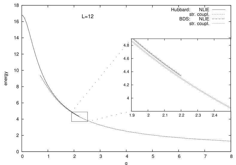
Figure 4: The behaviour of the energies $E(g)$ and $E_{\text{BDS}}$ from small to strong coupling is plotted here for a lattice of 12 sites. The left branches of the curves are the same as in Fig. 3 while the right branches are given by the strong coupling expansions (8.6). In the small picture there is a zoom of the region where the branches overlap.

Figure 5: Comparison of Hubbard and BDS energies (anomalous dimensions) for $L=40$. The two curves are visibly hard to distinguish in this range of $g$. The largest reached absolute difference is 0.0038 namely a relative difference of $0.019\%$.

Let us begin with $L=12$. Figure 3 shows that already at such a small value of $L$, and beyond the perturbative region in the coupling $g$, the curves computed by means of both BDS Ansatz and Hubbard model overlap almost completely. This is an indication that even if we are dealing with a chain which is far from the thermodynamic limit, the predictions of the BDS Ansatz can be considered as a good effective approximation of the Hubbard model behaviour.

Hence, even if the BDS Ansatz is plagued by the wrapping problem, at a quantitative level it is able to reproduce all the significant features of the Hubbard model, beginning from $L\simeq 12$.

Again, we use eqs. (7) to describe the strong coupling behaviour

$$E = \frac{10.8347}{g}-\frac{3}{g^{2}}+\dots$$

$$E_{\text{BDS}} = \frac{10.8038}{g}-\frac{3}{g^{2}}+\dots.$$ (8.6)

The behaviour from weak to strong coupling for both the Hubbard model and the BDS anstaz is plotted in Fig. 4: the left branches are the same as in Fig. 3 (numerical solution of the NLIEs), while the right branches are given by the equations (8.6) (strong coupling expansions). As we stated at the end of previous subsection, left and right branches smoothly join.

Let us remark that it was quite unexpected to find the observed good agreement between the Hubbard model and the BDS Ansatz predictions for such a small value of $L$. It is also important to stress the crucial role played by the NLIEs in order to obtain the exact behaviour of the energy outside the perturbative domain. As shown in the study of the anomalous dimension of the Konishi operator, the perturbation theory alone is not enough to reach an overlap with the strong coupling expansion.

Finally, we compared the Hubbard and BDS anomalous dimensions for $L=40$ in the range $g\in[0,3]$: as expected, the agreement between them is further enhanced and the two curves can be hardly distinguished, see Fig. 5.

The interesting feature of this case is that we were able to explicitly follow the evolution of the relative difference between Hubbard and BDS from weak to strong coupling. We observed that the two curves begin to separate at small $g$, then they achieve a maximum in the relative difference, and after that they start to approach again. We think that such a pattern is valid at any $L$, but the reduced numerical precision does not allow us to observe it for smaller values of $L$.

Remark. The fact that $E_{\text{BDS}}>E$ at weak coupling, but $E_{\text{BDS}}<E$ at strong coupling suggests that the curves will cross at some intermediate value of $g$. This is consistent with our numerical observation of the approaching of them as $g$ increases. Unfortunately, the reduced precision of our data at large $g$ prevented us to observe such a crossing explicitly.

8.3 Large operators at fixed $g$

Table 1: Table of data concerning the exponential damping $|E_{\text{BDS}}-E|\propto e^{-a(g)L}$ as in (8.7) and in Section 5. Two significant digits are available for the data obtained by numerical integration of the NLIEs namely for $a(g)$. The inequality (8.8) is satisfied with a slowly changing or possibly constant ratio.

$$\begin{array}[]{r|ccc}g&1.2&1.6&2\\ \hline\cr a(g)&0.0076&0.0011&0.00017\\ \omega(g)&0.0174422&0.00342347&0.000649349\\ \epsilon_{M}&0.290524&0.219211&0.175869\\ \epsilon_{M}\omega(g)&0.00506738&0.000750462&0.000114200\\ \frac{a(g)}{\epsilon_{M}\,\omega(g)}&1.5&1.5&1.5\end{array}$$

Figure 6: Difference between the highest Hubbard and BDS energies (anomalous dimensions) at different sizes of the system and at two fixed values of the coupling, $g=1.2$ and $g=2$. A logarithmic scale is used on the vertical axis. The linear behaviour is clear indication of the exponential damping discussed in Section 5 and summarized in (8.7). Related numerical data are provided in Table 1.

Another interesting analysis concerns the difference between the highest energies of Hubbard and BDS as a function of $L$ and at fixed coupling. Our choices were the values $g=1.2,~{}1.6$ and $g=2$, which lie in an intermediate region for which our asymptotic result (5.30) does not apply. The solution of our NLIEs gives the result depicted in Table 1 and in Fig. 6 on a log diagram: for large $L$ ($L>300$) the behaviour is linear, meaning that the difference between the energies decays exponentially as the length $L$ is increased. This confirms our analytical findings of Section 5. Consistently with that Section, we introduce the numerical rate of decay $a(g)$ and write

$$|E_{\text{BDS}}-E|\propto e^{-a(g)L}\,,\qquad a(g)>0\,.$$ (8.7)

According to our results of Section 5, the inequality

$$\epsilon\,\omega(g)\leq\epsilon_{M}\,\omega(g)\leq a(g)\,$$ (8.8)

must hold and in this respect, Table 1 suggests that (8.8) is actually correct for the values of $g$ chosen.

The values of $a(g)$ shown in Table 1 interpolate between the behaviour at small $g$, $a(g)=-2\ln g$, and at large $g$, $a(g)=\frac{1}{\sqrt{2}g}$. Consistently, the values of $a(g)$ in Table 1 decrease as $g$ increases. However, understanding how $a(g)$ passes from the small coupling to the large coupling behaviour on the basis of numerical data seems difficult. Indeed, the comparison of the two plots in Fig. 6 shows that the exponential behaviour in $L$ of $E-E_{\text{BDS}}$ is strongly dependent on the actual value of the coupling. In addition, it is clear that linearity (i.e. exponential damping) is reached at values of $L$ which rapidly increase with $g$.

Figure 7: The finite size correction $1/L$ is compared with the theoretical BDS prediction (5.21), represented with the dashed straight line. As observed in Fig. 6, for higher values of $g$ linearity is reached at higher values of L.

Finally, we remember, as pointed out before equation (5.21), that the exponential damping of $E-E_{\text{BDS}}$ forces the equality of logarithmic-like and power-like finite size corrections in the Hubbard and BDS models. The most relevant case is the $1/L$ behaviour, that is explicitly plotted for the Hubbard model in Fig. 7 and compared with the analytical prediction (5.21) coming from the BDS Ansatz.

9 Summary and perspective

In this paper we have derived the NLIEs describing the highest energy state of the half-filled (attractive) Hubbard model with and without a suitable flux which is responsible for a precise contact with the highest possible anomalous dimension (at fixed bare dimension $L$). In particular, according to the important correspondence pioneered in [12], we computed the energy/anomalous dimension for this state/operator, and all the other conserved quantity eigenvalues may find an exact expression. The dimension is of course a function of the ’t Hooft coupling $\lambda$ (and of the operator bare dimension $L$), thanks to a duality connexion between this latter and the Hubbard coupling. While exact analytical formulæ  for energy/dimension have been extracted only in the strong and weak coupling perturbative regime, numerical solutions of the NLIEs and corresponding energy values can be obtained for arbitrary values of $g$ and $L$. In this respect, we have been able to provide many plots showing clearly the dependence of the highest energy (anomalous dimension) on the coupling $g$. In particular, we have concentrated ourselves on the comparison with the highest energy of the (simpler) BDS model. We have shown, first analytically then numerically, that at large sizes ($L\rightarrow\infty$), they coincide up to corrections exponentially small (i.e. $o(L^{-\infty}$)), i.e. of non-analytic form. Of course, the finite size corrections are also important in the string theory since they come out as quantum loop corrections. As regards future perspectives, we would like to stress that the NLIE approach is a very good and effective method to provide the observables dependence on the model parameters and size. One good quality is that the NLIE can be written whenever the Bethe Ansatz equations are available, and even under more general circumstances, thanks to its equivalence to some functional equations. In particular the application of the NLIE to the so-called string Bethe Ansatz [14] and larger field sectors is particularly desirable, in view of tests of the AdS/CFT correspondence. For the time being, indeed, in spite of the progress following the discovery of integrability in both sides of the duality, such tests could be performed only for a limited number of cases, because of the technical difficulty in handling the Bethe equations for general length and coupling. In the previous work [16] and in the present one we have showed that by means of the NLIE framework we are able to overcome this difficulty and provide exact analytic scaling with the length $L$ and the coupling $\lambda$ (and also numerical evaluation of the conformal dimensions).

References

• [1] A. Kapustin, E. Witten, Electric-Magnetic Duality and the Geometric Langlands Program, hep-th/0604151;
• [2] J.M. Maldacena, The large N limit of superconformal field theories and supergravity, Adv. Theor. Math. Phys. 2 (1998) 231 and hep-th/9711200;
E. Witten, Anti-de Sitter space and holography, Adv. Theor. Math. Phys. 2 (1998) 253 and hep-th/9802150;
S.S. Gubser, I.R. Klebanov, A.M. Polyakov, Gauge theory correlators from non-critical string theory, Phys.Lett. B428 (1998) 105 and hep-th/9802109;
• [3] J.A. Minahan, K. Zarembo, The Bethe Ansatz for ${\cal N}=4$ Super Yang-Mills, JHEP03 (2003) 013 and hep-th/0212208;
• [4] H. Bethe, On the theory of metals, 1. Eigenvalues and eigenfunctions for the linear atomic chain, Z. Phys. 71 (1931) 205;
• [5] R. Hernandez, E. Lopez, A. Perianez, G. Sierra, Finite size effects in ferromagnetic spin chains and quantum corrections to classical strings, JHEP06 (2005) 011 and hep-th/0502188;
• [6] N. Beisert, A.A. Tseytlin, K. Zarembo, Matching quantum strings to quantum spins: one-loop vs. finite size corrections, Nucl. Phys. B715 (2005) 190 and hep-th/0502173;
• [7] N. Gromov, V. Kazakov, Double scaling and Finite Size Corrections in $sl(2)$ Spin Chain, Nucl. Phys. B736 (2006) 224 and hep-th/0510194;
• [8] D. Berenstein, J.M. Maldacena, H. Nastase, Strings in flat space and pp waves from ${\cal N}=4$ super Yang-Mills, JHEP 04 (2002) 013 and hep-th/0202021;
• [9] N. Beisert, C. Kristjansen, M. Staudacher, The dilatation operator of ${\cal N}=4$ super Yang-Mills theory, Nucl. Phys. B664 (2003) 131 and hep-th/0303060;
• [10] D. Serban, M. Staudacher, Planar ${\cal N}=4$ gauge theory and the Inozemtsev long range spin chain, JHEP06 (2004) 001 and hep-th/0401057;
• [11] N. Beisert, V. Dippel, M. Staudacher, A novel long range spin chain and planar ${\cal N}=4$ super Yang-Mills, JHEP07 (2004) 075 and hep-th/0405001;
• [12] A. Rej, D. Serban, M. Staudacher, Planar ${\cal N}=4$ gauge theory and the Hubbard model, JHEP03 (2006) 018 and hep-th/0512077;
• [13] J.A. Minahan, Strong coupling from the Hubbard model, J.Phys.A39 (2006) 13083 and hep-th/0603175;
• [14] N. Beisert, B. Eden, M. Staudacher, Trascendentality and Crossing, hep-th/0610251;
• [15] E.H. Lieb, F.Y. Wu, Absence of Mott-transition in an exact solution of the short-range, one-band model in one dimension, Phys. Rev. Lett. 20 (1968) 1445;
E.H. Lieb, F.Y. Wu, The one-dimensional Hubbard model: A reminiscence, cond-mat/0207529;
• [16] G.Feverati, D.Fioravanti, P.Grinza, M.Rossi, On the finite size corrections of anti-ferromagnetic anomalous dimensions in ${\cal N}=4$ SYM, JHEP05 (2006) 068 and hep-th/0602189;
• [17] P.A. Pearce, A. KlΓΌmper, Finite-size corrections and scaling dimensions of solvable lattice models: an analytic method, Phys. Rev. Lett. 66, volume 8 (1991) 974;
A. KlΓΌmper, M.T. Batchelor and P.A. Pearce, Central charges of the 6- and 19-vertex models with twisted boundary conditions, J. Phys. A24 (1991) 3111;
• [18] C. Destri, H.J. de Vega, New thermodynamic Bethe Ansatz equations without strings, Phys. Rev. Lett. 69 (1992) 2313;
C. Destri, H.J. de Vega, Unified approach to Thermodynamic Bethe Ansatz and finite size corrections for lattice models and field theories, Nucl. Phys. B438 (1995) 413 and hep-th/9407117;
• [19] D. Fioravanti, A. Mariottini, E. Quattrini, F. Ravanini, Excited state Destri-de Vega equation for sine-Gordon and restricted sine-Gordon models, Phys. Lett. B390 (1997) 243 and hep-th/9608091;
C. Destri, H.J. de Vega, Non linear integral equation and excited–states scaling functions in the sine-Gordon model, Nucl. Phys. B504 (1997) 621 and hep-th/9701107;
• [20] J. Hubbard, Electron correlation in narrow energy bands, Proc. Roy. Soc. (London) A276 (1963) 238;
• [21] E. Ercolessi, G. Morandi, A. M. Srivastava, A. P. Balachandran, The Hubbard Model and Anyon Superconductivity, World Scientific;
• [22] A.KlΓΌmper, R.Z. Bariev, Exact thermodynamics of the Hubbard chain: free energy and correlation lengths, Nucl. Phys. B458 (1996) 623;
• [23] G. JΓΌttner, A. KlΓΌmper, J.Suzuki, The Hubbard chain at finite temperatures: ab initio calculations of Tomonaga-Luttinger liquid properties, Nucl. Phys. B522 (1998) 471 and cond-mat/9711310;
• [24] T. Deguchi, F. H. L. Essler, F. GΓΆhmann, A. KlΓΌmper, V. E. Korepin, K. Kusakabe, Thermodynamics and excitations of the one-dimensional Hubbard model, Phys. Rep. 331 (2000) 197 and cond-mat/9904398;
• [25] D. Fioravanti, M. Rossi, From finite geometry exact quantities to (elliptic) scattering amplitudes for spin chains: the 1/2-XYZ, JHEP08(2005) 010 and hep-th/0504122;
• [26] M. Takahashi, Thermodynamics of one-dimensional solvable models, Cambridge University Press;
• [27] F. Woynarovich, H.P. Eckle, Finite-size corrections for the low lying states of a half-filled Hubbard chain, J. Phys. A 20 (1987) L443;
• [28] S. SchΓ€fer-Nameki, M. Zamaklar, K. Zarembo, How accurate is the quantum string Bethe Ansatz, hep-th/0610250;
• [29] P.W. Anderson, New Approach to the Theory of Superexchange Interactions, Phys. Rev. 115 (1959) 2;
• [30] I.S. Gradshteyn, I.M. Ryzhik, Table of integrals, series and products, Academic Press;
• [31] E.N. Economou, P.N. Poulopoulos, Ground state energy of the half-filled one-dimensional Hubbard model, Phys. Rev. B20 (1979) 4756;
• [32] W. Metzner, D. Vohllhardt, Ground state energy of the $d=1,2,3$ dimensional Hubbard model in the weak-coupling limit, Phys. Rev. B39 (1989) 4462;
• [33] M. Beccaria, C. Ortix, Strong coupling anomalous dimensions of ${\cal N}=4$ super Yang-Mills, JHEP 0609 (2006) 016 and hep-th/0606138;
• [34] M. Beccaria, C. Ortix, AdS/CFT duality at strong coupling, hep-th/0610215.