Eikonal Approximation in AdS/CFT:
Conformal Partial Waves and Finite N Four–Point Functions

Abstract:

We introduce the impact parameter representation for conformal field theory correlators of the form $\mathcal{A}\sim\left\langle\mathcal{O}_{1}\mathcal{O}_{2}\mathcal{O}_{1}\mathcal{O}_{2}\right\rangle$. This representation is appropriate in the eikonal kinematical regime, and approximates the conformal partial wave decomposition in the limit of large spin and dimension of the exchanged primary. Using recent results on the two–point function $\left\langle\mathcal{O}_{1}\mathcal{O}_{1}\right\rangle_{\textrm{shock}}$ in the presence of a shock wave in Anti–de Sitter, and its relation to the discontinuity of the four–point amplitude $\mathcal{A}$ across a kinematical branch cut, we find the high spin and dimension conformal partial wave decomposition of all tree–level Anti–de Sitter Witten diagrams. We show that, as in flat space, the eikonal kinematical regime is dominated by the T–channel exchange of the massless particle with highest spin (graviton dominance). We also compute the anomalous dimensions of the high spin $\mathcal{O}_{1}\mathcal{O}_{2}$ composites. Finally, we conjecture a formula re–summing crossed–ladder Witten diagrams to all orders in the gravitational coupling.

1 Introduction and Summary

The AdS/CFT correspondence opens the fascinating possibility of describing quantum gravitational interactions using gauge theories and vice–versa [1, 2, 3, 4, 5]. When the radius $\ell$ of Anti–de Sitter (AdS) is much larger than the string length, the correspondence relates a local gravitational theory, describing the dynamics of string massless modes in AdS, to a strongly coupled gauge theory defined on the AdS boundary. The perturbative expansion in the AdS gravitational coupling $G$ corresponds, in general, to the $1/N$ expansion in the gauge theory. However, the understanding of loop corrections in AdS quantum gravity is presently beyond our reach and it is therefore difficult to check the correspondence beyond the planar limit or to use it to derive finite $N$ effects of strongly coupled gauge theories. In flat space, where similar problems are present, it is nonetheless possible to re–sum the gravitational loop expansion when considering four–point amplitudes in the specific eikonal kinematical regime. In a companion paper [6], we generalize the eikonal approximation to the calculation of four–point amplitudes in AdS spaces. In the sequel, we shall explore the consequences of these results for the dual conformal field theory (CFT), therefore initiating a program to probe finite $N$ effects of strongly coupled gauge theories.

We shall concentrate on CFT correlators like $\mathcal{A}\sim\left\langle\mathcal{O}_{1}\mathcal{O}_{2}\mathcal{O}_{1}\mathcal{O}_{2}\right\rangle$, which can in general be decomposed in conformal partial waves in various channels, thus giving information about the CFT spectrum and three–point couplings. Neglecting string corrections, these correlators can be computed gravitationally using Witten diagrams, which describe interactions in AdS. Unfortunately, it is a hard problem to decompose a given AdS diagram in conformal partial waves and therefore to improve our understanding of the dual CFT. Recall that, in flat space, the eikonal kinematical regime of small scattering angle controls the large spin behavior of the partial wave decomposition. Analogously, we shall use the results derived in [6] to prove a similar result in AdS. We will show, in particular, how to determine directly the high spin and dimension decomposition of tree–level Witten diagrams and how to compute the anomalous dimensions of certain high spin composite operators.

Let us recall some relevant facts on the eikonal formalism in flat space. Consider the scattering of two scalar particles in flat Minkowski space $\mathbb{M}^{d+1}$, working at high energies and neglecting particles masses. The scattering amplitude $\mathcal{A}$ is a function of the Mandelstam invariants $s$, $t$, and can be conveniently decomposed in S–channel partial waves

$$\mathcal{A=}s^{\frac{3-d}{2}}~{}\sum_{J\geq 0}\mathcal{S}_{J}\left(z\right)~{}e^{-2\pi i\,\sigma_{J}\left(s\right)}~{},$$

with

$$z=\sin^{2}\left(\frac{\theta}{2}\right)=-\frac{t}{s}$$

related to the scattering angle $\theta$ and with $\sigma_{J}\left(s\right)$ the phase shift for the spin $J$ partial wave. The angular functions $\mathcal{S}_{J}\left(z\right)$ are eigenfunctions of the Laplacian on the sphere at infinity, with eigenvalue $-J\left(J+d-2\right)$, and are polynomials in $z$ of order $J$, whose explicit form depends on the dimension of spacetime. They can be written as hypergeometric functions

$$\mathcal{S}_{J}\left(z\right)\propto F\left.\left(-J,J+d-2,\frac{d-1}{2}\right|z\right).$$

and they are normalized so that $\sigma=0$ corresponds to free propagation with no interactions. Unitarity then implies $\mathrm{Im}\,\sigma\leq 0$. The amplitude itself can be computed in perturbation theory

$$\mathcal{A}=\mathcal{A}_{0}+\mathcal{A}_{1}+\cdots~{},$$

where $\mathcal{A}_{0}=s^{\frac{3-d}{2}}\sum_{J}\mathcal{S}_{J}\left(z\right)~{}$ corresponds to graph $\left(a\right)$ in figure 1 describing free propagation in spacetime. All S–channel partial waves contribute to $\mathcal{A}_{0}$ with equal weight one, and vanishing phase shift.

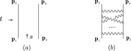
Figure 1: In the eikonal regime, free propagation $\left(a\right)$ is modified primarily by interactions described by crossed–ladder graphs $\left(b\right)$.

In the eikonal regime we are interested in the limit $z\ll 1$ of small scattering angle, where the amplitude is dominated by partial waves with large intermediate spin $J$. One may then replace the sum over $J$ with an integral over the impact parameter $r$,

$$\frac{r}{2}=\frac{J}{\sqrt{s}}~{},$$

denoting the phase shifts by $\sigma\left(s,r\right)$ from now on. More precisely, if we consider the double limit

$$z\rightarrow 0\,,~{}\ \ \ \ \ \ J\rightarrow\infty\,,~{}\ \ \ \ \ \ \ \ \ \ \ \ \ \left(z\sim J^{-2}\right),$$ (1.1)

we may approximate the sphere at infinity by a transverse euclidean plane $\mathbb{E}^{d-1}$ and the angular functions $\mathcal{S}_{J}\left(z\right)$ become, in this limit, the impact parameter partial waves $\mathcal{I}_{J}$,

$$\mathcal{I}_{J}\propto\int_{\mathbb{E}^{d-1}}~{}dx~{}\delta\left(x^{2}-r^{2}\right)~{}e^{iq\cdot x}~{}\propto z^{\frac{3-d}{4}}\,\mathbf{J}_{\frac{d-3}{2}}\left(2J\sqrt{z}\right),$$ (1.2)

with $q^{2}=-t$ and $\mathbf{J}_{\nu}$ the Bessel function. One then obtains the impact parameter representation of the amplitude

$$\mathcal{A}\,\simeq\,2s\int_{\mathbb{E}^{d-1}}~{}dx\;e^{iq\cdot x}\;e^{-2\pi i\,\sigma\left(s,r\right)}\,,$$ (1.3)

where $r=\sqrt{x^{2}}$. In general, the phase shift receives contributions at all orders in perturbation theory. On the other hand, the leading behavior of $\sigma\left(s,r\right)$ for large $r$, which controls small angle scattering, is uniquely dominated by the leading tree–level interaction $\mathcal{A}_{1}$ and it is therefore determined by a simple Fourier transform

$$\mathcal{A}_{1}\,\simeq\,-4\pi i~{}s\int_{\mathbb{E}^{d-1}}~{}dx\;e^{iq\cdot x}\;\sigma(s,r)\,.$$ (1.4)

The main result of the eikonal approximation is that the knowledge of the tree–level amplitude $\mathcal{A}_{1}$ is enough to compute the amplitude (1.3) in the $z\rightarrow 0$ limit to all orders in the coupling. Moreover, the dominant interaction in $\mathcal{A}_{1}$ comes from T–channel exchanges of spin $j$ massless particles, so that the full amplitude (1.3) approximately re–sums the crossed–ladder graphs in figure 1$(b)$. In the limit of high energy $s$, the mediating particle with maximal $j$ dominates the interaction. In theories of gravity, this particle is the graviton, with $j=2$.

To understand in more detail the generic behavior of amplitudes for small scattering angle and large energies, consider some sample interactions shown in figure 2 contributing to $\mathcal{A}_{1}$, where the exchanged particle has spin $j$.

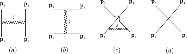
Figure 2: Some possible interactions at tree–level, both in flat space and in $\mathrm{AdS}$. When decomposing the amplitude in the $S$–channel, only graph $(a)$, with maximal spin $j=2$, dominates the dynamics at large intermediate spin and energy.

The contribution of graph $2(a)$ to $\mathcal{A}_{1}$ has the form

$$4^{3-j}~{}2\pi i\,G~{}\frac{s^{j}-c_{1}s^{j-1}t+\cdots}{-t}\propto s^{j-1}\left(\frac{1}{z}+c_{1}+\cdots+c_{j}z^{j-1}\right).$$

The polynomial part in $z$ contributes to partial waves with spin $J<j$. This can also be understood in the impact parameter representation (1.4), since polynomial terms in $z=q^{2}s$ give, after Fourier transform, delta function contributions to the phase shift localized at $r=0$. The universal term $s^{j-1}/z$ contributes, on the other hand, to partial waves of all spins and gives a phase shift at large $r$ given by

$$\sigma\left(s,r\right)\simeq-8G\left(\frac{s}{4}\right)^{j-1}\Pi\left(r\right)~{},$$ (1.5)

where $\Pi\left(r\right)$ is the massless Euclidean propagator in transverse space $\mathbb{E}^{d-1}$. At high energies, the maximal $j$ dominates. Graph $2(b)$ is obtained by interchanging the role of $s$ and $t$, and therefore is proportional to $s^{j-1}\left(z^{j}+c_{1}z^{j-1}+\cdots+c_{j}\right)$. The corresponding intermediate partial waves have spin $J\leq j$. Finally, graph $2(c)$ is obtained from $2(a)$ by replacing $t$ by $u=-\left(s+t\right)$ and therefore by sending $z\rightarrow 1-z$. Using the fact that $\mathcal{S}_{J}(1-z)=(-)^{J}\mathcal{S}_{J}(z)$, we can again expand the U–channel exchange graph $2(c)$ in the form $s^{\frac{3-d}{2}}\sum_{J}\left(-\right)^{J}\mathcal{S}_{J}~{}\sigma_{J}\left(s\right)$ where $\sigma_{J}(s)$ are the phase shifts of the T–channel exchange, whose large spin behavior is given by (1.5). At large spins, the contribution to the various partial waves is alternating in sign and averages to a sub–leading contribution. Finally, the contact graph $2(d)$ only contains a spin zero contribution. We conclude that, at large spins and energies, the T–channel exchange of a graviton in graph $2(a)$ dominates all other interactions.

We shall study the CFT analogue of $2\rightarrow 2$ scattering of scalars in flat space. More precisely, we will study the CFT correlator

$$\left\langle\mathcal{O}_{1}\left(\mathbf{p}_{1}\right)\mathcal{O}_{2}\left(\mathbf{p}_{2}\right)\mathcal{O}_{1}\left(\mathbf{p}_{3}\right)\mathcal{O}_{2}\left(\mathbf{p}_{4}\right)\right\rangle_{\text{{CFT}}_{d}}\equiv\frac{1}{\mathbf{p}_{13}^{\Delta_{1}}\mathbf{p}_{24}^{\Delta_{2}}}\,\,\mathcal{A}\left(z,\bar{z}\right)~{},$$

where the scalar primary operators $\mathcal{O}_{1}$, $\mathcal{O}_{2}$ have conformal dimensions $\Delta_{1}$, $\Delta_{2}$, respectively. The $\mathbf{p}_{i}$ are now points on the boundary of $\mathrm{AdS}$, and the amplitude $\mathcal{A}$ is now a function of two cross–ratios $z$, $\bar{z}$, whose precise definition is given in section 2. Neglecting string effects, the function $\mathcal{A}$ can be computed in the dual $\mathrm{AdS}$ formulation as a field theoretic perturbation series in the gravitational coupling [2, 3, 4, 7, 8]

$$\mathcal{A}=\mathcal{A}_{0}+\mathcal{A}_{1}+\cdots~{},$$

where $\mathcal{A}_{0}=1$ corresponds to free propagation described again in figure 1$(a)$. The amplitude $\mathcal{A}$ can be decomposed, as in flat space, in S–channel partial waves. These are know, in the CFT litterature, as conformal partial waves and correspond to the exchange of the conformal primaries that appear in the operator product expansion (OPE) of $\mathcal{O}_{1}$ with $\mathcal{O}_{2}$ as $\mathbf{p}_{1}\rightarrow\mathbf{p}_{2}$, together with their descendants. In particular, the free amplitude $\mathcal{A}_{0}$ corresponds to the exchange of an infinite set of $\mathcal{O}_{1}\partial_{\mu_{1}}\cdots\partial_{\mu_{J}}\partial^{2n}\mathcal{O}_{2}$ composites of spin $J$ and dimension $E=\Delta_{1}+\Delta_{2}+J+2n$, with $J,n$ non–negative integers.

As the coupling is turned on, we expect that the above lattice of intermediate primaries acquires anomalous dimensions, and also that new intermediate states appear in the partial wave decomposition. We shall show that the large spin and dimension S–channel decomposition of the tree level amplitude $\mathcal{A}_{1}$ is dominated, as in flat space, by the T–channel exchange of massless particles of maximal spin $j$. In fact, in this limit, this decomposition is determined by the small $z$, $\bar{z}$ behavior of the discontinuity across a kinematical branch cut of the T–channel exchange Witten diagram 2$(a)$, which we derived in [6]. This result is central in the derivation of our main findings:

• The AdS graph 2$(a)$ contributes to all partial waves corresponding to the $\mathcal{O}_{1}\partial^{N}\mathcal{O}_{2}$ composites of spin $J$ and dimension $E$ already present in $\mathcal{A}_{0}$. For large $E$, $J$ these composites acquire anomalous dimensions given by

  $$2\sigma\left(s,r\right)~{},$$

  where $\sigma\left(s,r\right)$ is again given by (1.5), but where now

  $$s =\left(E^{2}-J^{2}\right)/\ell^{2}~{},$$

  $$\tanh\left(\frac{r}{2\ell}\right) =\frac{J}{E}~{},$$

  and where $\Pi\left(r\right)$ is the massive Euclidean propagator on transverse space, which is now the hyperbolic space $\mathrm{H}_{d-1}$ with radius $\ell$. The mass–squared is given by $\left(d-1\right)/\ell^{2}$ and $r$ is the geodesic distance on $\mathrm{H}_{d-1}$. Once again, the dominant contribution to $\sigma$ comes from the exchange of the graviton. Note that the flat space limit can be obtained letting $\ell\rightarrow\infty$ keeping the physical $\mathrm{AdS}$ energy $E/\ell$ fixed. (Sections 4.2 and 5)

• The AdS graph 2$(b)$ contributes to partial waves with spin $J\leq j$ and with dimensions $E=d$, $E=\Delta_{1}+\Delta_{2}+n$. These partial waves correspond to the massless exchanged particle and to corrections to the composites $\mathcal{O}_{1}\partial^{N}\mathcal{O}_{2}$ with bounded spin. Moreover, the contribution with maximal spin $J=j$ can be determined explicitly without computing the full graph. (Sections 4.3 and 5)

• The AdS graph 2$(c)$ is similar to graph 2$(a)$, but with alternating signs $\left(-\right)^{J}$. Graph 2$(d)$ contributes to partial waves with spin $J=0$ only. Comments similar to the flat space case apply. (Section 5)

• In order to arrive at the above results, we have extended the impact parameter representations (1.2) and (1.4) to the decomposition of $\mathrm{CFT}$ amplitudes in terms of conformal partial waves, using the approach of [9, 10]. (Section 3.2)

Finally, in section 6, we conjecture a formula for $\mathcal{A}$ which resums the perturbative expansion in the AdS gravitational coupling $G$ in the eikonal limit. This formula also predicts the anomalous dimensions of $\mathcal{O}_{1}\partial^{N}\mathcal{O}_{2}$ composites with large spin and conformal dimension to all orders in $G$.

2 Preliminaries and Notation

This section follows closely section 2 of [6] and is included for completeness. Recall that AdS_d+1 space, of dimension $d+1$, can be defined as a pseudo–sphere in the embedding space $\mathbb{M}^{2}\times\mathbb{M}^{d}$. We denote with $\mathbf{x}=\left(x^{+},x^{-},x\right)$ a point in $\mathbb{M}^{2}\times\mathbb{M}^{d}$, where $x^{\pm}$ are light–cone coordinates on $\mathbb{M}^{2}$ and $x$ denotes a point in $\mathbb{M}^{d}$. Then, the AdS space of radius $\ell$ is described by

$$\mathbf{x}^{2}=-x^{+}x^{-}+x^{2}=-\ell^{2}~{}.$$ (2.6)

Similarly, a point on the holographic boundary of AdS_d+1 can be described by a ray on the light–cone in $\mathbb{M}^{2}\times\mathbb{M}^{d}$, that is by a point $\mathbf{p}$ with

$$\mathbf{p}^{2}=-p^{+}p^{-}+p^{2}=0~{},$$

defined up to re–scaling

$$\mathbf{p}\sim\lambda\mathbf{p}\qquad\left(\lambda>0\right).$$

From now on we choose units such that $\ell=1$.

The AdS/CFT correspondence predicts the existence of a dual CFT_d living on the boundary of AdS_d+1. In particular, a CFT correlator of scalar primary operators located at points $\mathbf{p}_{1},\ldots,\mathbf{p}_{n}$ can be conveniently described by an amplitude

$$A\left(\mathbf{p}_{1},\ldots,\mathbf{p}_{n}\right)$$

invariant under $SO\left(2,d\right)$ and therefore only a function of the invariants

$$\mathbf{p}_{ij}=-2\mathbf{p}_{i}\cdot\mathbf{p}_{j}~{}.$$

Since the boundary points $\mathbf{p}_{i}$ are defined only up to re–scaling, the amplitude $A$ will be homogeneous in each entry

$$A\left(\ldots,\lambda\mathbf{p}_{i},\ldots\right)=\lambda^{-\Delta_{i}}A\left(\ldots,\mathbf{p}_{i},\ldots\right)~{},$$

where $\Delta_{i}$ is the conformal dimension of the $i$–th scalar primary operator.

Throughout this paper we will focus our attention on four–point amplitudes of scalar primary operators. More precisely, we shall consider correlators of the form

$$A\left(\mathbf{p}_{1},\mathbf{p}_{2},\mathbf{p}_{3},\mathbf{p}_{4}\right)=\left\langle\mathcal{O}_{1}\left(\mathbf{p}_{1}\right)\mathcal{O}_{2}\left(\mathbf{p}_{2}\right)\mathcal{O}_{1}\left(\mathbf{p}_{3}\right)\mathcal{O}_{2}\left(\mathbf{p}_{4}\right)\right\rangle_{\text{{CFT}}_{d}}$$

where the scalar operators $\mathcal{O}_{1},\mathcal{O}_{2}$ have dimensions

$$\Delta_{1}=\Delta+\nu~{},~{}\ \ \ \ \ \ \ \ \ \ \ \ \ \ \ \ \ \ \ \Delta_{2}=\Delta-\nu~{},$$

respectively. The four–point amplitude $A$ is just a function of two cross ratios $z,\bar{z}$ which we define, following [9, 10], in terms of the kinematical invariants $\mathbf{p}_{ij}$ as

$$z\bar{z} =\frac{\mathbf{p}_{13}\mathbf{p}_{24}}{\mathbf{p}_{12}\mathbf{p}_{34}}~{},$$

$$\left(1-z\right)\left(1-\bar{z}\right) =\frac{\mathbf{p}_{14}\mathbf{p}_{23}}{\mathbf{p}_{12}\mathbf{p}_{34}}~{}.$$

Then, the four–point amplitude can be written as

$$A\left(\mathbf{p}_{i}\right)=\frac{1}{\mathbf{p}_{13}^{\Delta_{1}}\mathbf{p}_{24}^{\Delta_{2}}}\,\,\mathcal{A}\left(z,\bar{z}\right)~{},$$

where $\mathcal{A}$ is a generic function of $z,\bar{z}$. By conformal invariance, we can fix the position of up to three of the external points $\mathbf{p}_{i}$. In what follows, we shall often choose the external kinematics by placing the four points $\mathbf{p}_{i}$ at

$$\mathbf{p}_{1} =\left(0,1,0\right)~{},\ \ \ \ \ \ \ \ \ \ \ \ \ \ \ \ \ \ \ \ \ \ \ \mathbf{p}_{2}=-\left(1,p^{2},p\right)~{},$$ (2.7)

$$\mathbf{p}_{3} =-\left(q^{2},1,q\right)~{},\ \ \ \ \ \ \ \ \ \ \ \ \ \ \ \ \ \ \ \mathbf{p}_{4}=\left(1,0,0\right)~{},$$

and we shall view the amplitude as a function of $p,q\in\mathbb{M}^{d}$. The cross ratios $z,\bar{z}$ are in particular determined by

$$z\bar{z}=q^{2}p^{2},~{}\ \ \ \ \ \ \ \ \ \ \ \ \ \ \ \ z+\bar{z}=2p\cdot q~{}.$$

When $d=2$ it is convenient to parameterize $\mathbb{M}^{d}$ by light–cone coordinates $x=x^{0}+x^{1}$, $\bar{x}=x^{0}-x^{1}$ with metric $-dxd\bar{x}$. Then, if we choose $p=\bar{p}=-1$ we have $q=z$, $\bar{q}=\bar{z}$.

In the sequel, we will denote with $\mathrm{H}_{d-1}\subset\mathbb{M}^{d}$ the transverse hyperbolic space, given by the upper mass–shell

$$x^{2}=-1~{},\ \ \ \ \ \ \ \ \ \ \ \ \ \ \left(x^{0}>0\right)$$

where $x\in\mathbb{M}^{d}$. We will also denote with $\mathrm{M}\subset\mathbb{M}^{d}$ the future Milne wedge given by $x^{2}\leq 0$,  $x^{0}\geq 0$. Similarly, we denote with $-\mathrm{M}$ the past Milne wedge and with $-\mathrm{H}_{d-1}$ the corresponding transverse hyperbolic space. Finally we denote with

$$\widetilde{dx}=2dx~{}\delta\left(x^{2}+1\right),$$

the volume element on $\mathrm{H}_{d-1}$, such that

$$\int_{\mathrm{M}}dx=\int_{\mathrm{M}}d(ty)\int_{0}^{\infty}t^{d-1}dt\int_{\mathrm{H}_{d-1}}\widetilde{dy}~{},$$

where $x=ty$ and $y\in\mathrm{H}_{d-1}$.

Throughout the paper, we will often need the massive Euclidean scalar propagator $\Pi\left(x,y\right)$ on $\mathrm{H}_{d-1}$, of mass–squared $d-1\,$, defined by

$$\left[\square_{\mathrm{H}_{d-1}}-\left(d-1\right)\right]\,\Pi\left(x,y\right)=-~{}\delta\left(x,y\right)~{},$$

and explicitly given in terms of the hypergeometric function

$$\Pi\left(x,y\right)=\left(4\pi\right)^{\frac{1-d}{2}}\frac{\Gamma\left(\frac{d+1}{2}\right)}{d(d-1)}\left(-z\right)^{1-d}F\left.\left(d-1,\frac{d+1}{2},d+1\right|\frac{1}{z}\right)\ ,$$ (2.8)

where $2z=1+x\cdot y$.

3 Conformal Partial Waves

The amplitude $\mathcal{A}\left(z,\bar{z}\right)$ can be expanded using the OPE around $z,\bar{z}=0,1,\infty$, corresponding to the point $\mathbf{p}_{3}$ getting close to $\mathbf{p}_{1}$, $\mathbf{p}_{2}$ and $\mathbf{p}_{4}$, respectively. In particular, we will be interested in the contribution to the amplitude $\mathcal{A}$ coming from the exchange of a conformal primary operator of dimension $E$ and integer spin $J\geq 0$ in the two channels

$$z,\bar{z} \rightarrow 0\ ,\ \ \ \ \ \ \ \ \ \ \ \ \ \ \ \ \ \ \ \ \ \ \text{\emph{T}--channel},$$

$$z,\bar{z} \rightarrow\infty\ ,\ \ \ \ \ \ \ \ \ \ \ \ \ \ \ \ \ \ \ \ \ \text{\emph{S}--channel},$$

together with all of its conformal descendants. It will be convenient in the following to use different labels for energy and spin $E,J$. We shall use most frequently conformal dimensions $h,\bar{h}$ defined by

$$E =h+\bar{h}~{},$$

$$J =h-\bar{h}~{}.$$

We will also use the so called impact parameter labels $s,r$ defined by

$$s =4h\bar{h}=E^{2}-J^{2}~{},$$

$$e^{-r} =\frac{\bar{h}}{h}=\frac{E-J}{E+J}~{}.$$ (3.9)

In terms of these variables, the present equations closely resemble eikonal results in flat space, with $s$ playing the role of the total center–of–mass energy squared, and with $r$ being the physical transverse impact parameter. We shall justify this interpretation more clearly in section 4.1. We also recall the unitarity bounds $E\geq d-2+J$ for $J\geq 1$ and $E\geq\left(d-2\right)/2$ for $J=0$, with the single exception of the vacuum with $E=J=0$. This translates into

$$\bar{h} \geq\frac{d-2}{2}~{},\ \ \ \ \ \ \ \ \ \ \ \ \ \ \ \ \ \ \ \ \left(J\geq 1\right),$$

$$\bar{h} \geq\frac{d-2}{4}~{},\ \ \ \ \ \ \ \ \ \ \ \ \ \ \ \ \ \ \ \ \left(J=0\right),$$

again with the exception of the vacuum at $h=\bar{h}=0$. Figure 3 summarizes the basic notation regarding the intermediate conformal primaries.

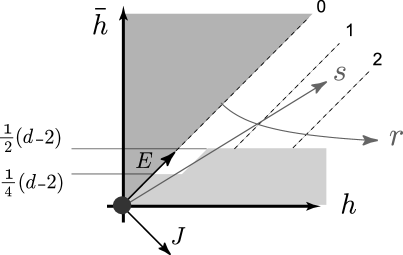
Figure 3: Intermediate primaries of dimension $E=h+\bar{h}$ and integer spin $J=h-\bar{h}\geq 0$ can exist in the white region along the dashed lines. The light grey region is excluded due to the unitarity constraint, with the vacuum at $h=\bar{h}=0$ being the unique exception. Also shown are the impact parameter labels $s=4h\bar{h}$ and $r=\ln\left(h/\bar{h}\right)$.

The amplitude $\mathcal{A}\left(z,\bar{z}\right)$ can be expanded in the basis of conformal partial waves in either the T or S–channels, whose elements we shall denote by

$$\mathcal{T}_{h,\bar{h}}~{}\left(z,\bar{z}\right)~{},\ \ \ \ \ \ \ \ \ \ \ \ \ \ \ \ \ \ \ \ \mathcal{S}_{h,\bar{h}}~{}\left(z,\bar{z}\right)~{}.$$

Following [9, 10], the functions $\mathcal{T}_{h,\bar{h}}$ and $\mathcal{S}_{h,\bar{h}}$ must be symmetric in $z,\bar{z}$ and must satisfy the differential equations

$$D_{T}~{}\mathcal{T}_{h,\bar{h}}=c_{h,\bar{h}}~{}\mathcal{T}_{h,\bar{h}}~{},$$

$$\left(z\bar{z}\right)^{\Delta}D_{S}~{}\left[\left(z\bar{z}\right)^{-\Delta}\mathcal{S}_{h,\bar{h}}\right]=c_{h,\bar{h}}~{}\mathcal{S}_{h,\bar{h}}~{},$$

where the constant $c_{h,\bar{h}}$ is the Casimir of the conformal group given by

$$c_{h,\bar{h}}=h\left(h-1\right)+\bar{h}\left(\bar{h}-d+1\right),$$

and where the differential operators $D_{T},~{}D_{S}$ have the explicit form

$$D_{T} =z^{2}\left(1-z\right)\partial^{2}-z^{2}\partial+\bar{z}^{2}\left(1-\bar{z}\right)\bar{\partial}^{2}-\bar{z}^{2}\bar{\partial}+$$ (3.10)

$$+\left(d-2\right)\frac{z\bar{z}}{z-\bar{z}}\left[\left(1-z\right)\partial-\left(1-\bar{z}\right)\bar{\partial}\right]$$

and

$$D_{S} =z\left(z-1\right)\partial^{2}+\left(2z-1\right)\partial+\frac{\nu^{2}}{z}+$$

$$+\bar{z}\left(\bar{z}-1\right)\bar{\partial}^{2}+\left(2\bar{z}-1\right)\bar{\partial}+\frac{\nu^{2}}{\bar{z}}+$$ (3.11)

$$+\frac{d-2}{z-\bar{z}}\left[z\left(z-1\right)\partial-\bar{z}\left(\bar{z}-1\right)\bar{\partial}\right]~{}.$$

Moreover, the partial waves $\mathcal{T}_{h,\bar{h}}$ and $\mathcal{S}_{h,\bar{h}}$ satisfy the boundary conditions

$$\lim_{z,\bar{z}\rightarrow 0}\mathcal{T}_{h,\bar{h}} \sim z^{h}~{}\bar{z}^{\bar{h}}~{},$$

$$\lim_{z,\bar{z}\rightarrow\infty}\mathcal{S}_{h,\bar{h}} \sim z^{\Delta-h}~{}\bar{z}^{\Delta-\bar{h}}~{},$$

where we choose to take the limit $\bar{z}\rightarrow 0,\infty$ first. The symmetric term with $h$ and $\bar{h}$ interchanged is then sub–leading since $h\geq\bar{h}$.

3.1 The $d=2$ Case

Explicit expressions for the partial waves $\mathcal{T}_{h,\bar{h}}$ and $\mathcal{S}_{h,\bar{h}}$ exist for $d$ even [9, 10], and are particularly simple in $d=2$ where the problem factorizes in left/right equations for $z$ and $\bar{z}$. In this case we have the explicit expressions

$$\mathcal{T}_{h,\bar{h}}\left(z,\bar{z}\right) =\mathcal{T}_{h}\left(z\right)\mathcal{T}_{\bar{h}}\left(\bar{z}\right)+\mathcal{T}_{\bar{h}}\left(z\right)\mathcal{T}_{h}\left(\bar{z}\right)~{},$$ (3.12)

$$\mathcal{S}_{h,\bar{h}}\left(z,\bar{z}\right) =\mathcal{S}_{h}\left(z\right)\mathcal{S}_{\bar{h}}\left(\bar{z}\right)+\mathcal{S}_{\bar{h}}\left(z\right)\mathcal{S}_{h}\left(\bar{z}\right)~{},$$

for $h>\bar{h}$ and

$$\mathcal{T}_{h,h}\left(z,\bar{z}\right) =\mathcal{T}_{h}\left(z\right)\mathcal{T}_{h}\left(\bar{z}\right)~{},$$

$$\mathcal{S}_{h,h}\left(z,\bar{z}\right) =\mathcal{S}_{h}\left(z\right)\mathcal{S}_{h}\left(\bar{z}\right)~{},$$

for $h=\bar{h}$, where

$$\mathcal{T}_{h}\left(z\right) =\left(-z\right)^{h}~{}F\Big{(}h,h,2h\Big{|}z\Big{)}~{},$$

$$\mathcal{S}_{h}\left(z\right) =a_{h}~{}\left(-z\right)^{\Delta-h}~{}F\Big{(}h+\nu,h-\nu,2h\Big{|}z^{-1}\Big{)}~{}.$$ (3.13)

The specific normalization of the S–channel partial waves

$$a_{h}=\frac{\Gamma\left(h+\nu\right)\Gamma\left(h-\nu\right)\Gamma\left(h+\Delta-1\right)}{\Gamma\left(\Delta+\nu\right)\Gamma\left(\Delta-\nu\right)\Gamma\left(2h-1\right)\Gamma\left(h-\Delta+1\right)}$$

is chosen for later convenience, and it is such that

$$\sum_{h\in\Delta+\mathbb{N}_{0}}\mathcal{S}_{h}\left(z\right)=1~{},$$ (3.14)

where $\mathbb{N}_{0}$ is the set of non–negative integers.

It is clear from (3.12) that the $h,\bar{h}$ partial waves correspond to the exchange of a pair of primary operators of holomorphic/antiholomorphic dimension $\left(h,\bar{h}\right)$ and $\left(\bar{h},h\right)$, together with their descendants.

3.2 Impact Parameter Representation

We now move back to general dimension $d$, and we consider the behavior of the S–channel partial waves $\mathcal{S}_{h,\bar{h}}\left(z,\bar{z}\right)$ for $z,\,\bar{z}\to 0$, i.e., in the dual T–channel. More precisely, in strict analogy with the case of flat space, we analyze the double limit

$$z,\bar{z} \rightarrow 0~{},$$

$$h,\bar{h} \rightarrow\infty~{},$$

as in (1.1), with

$$z\sim\bar{z}\sim h^{-2}\sim\bar{h}^{-2}~{}.$$

In this limit, the differential operator $D_{S}$ in (3.11) and the constant $c_{h,\bar{h}}$ reduce to

$$-\tilde{D}_{S}=z\partial^{2}+\bar{z}\bar{\partial}^{2}+\partial+\bar{\partial}-\frac{\nu^{2}}{z}-\frac{\nu^{2}}{\bar{z}}+\frac{d-2}{z-\bar{z}}\left(z\partial-\bar{z}\bar{\partial}\right)~{}$$

and

$$\tilde{c}_{h,\bar{h}}=h^{2}+\bar{h}^{2}~{}.$$

We shall denote with $\mathcal{I}_{h,\bar{h}}\left(z,\bar{z}\right)$ the approximate impact parameter S–channel partial wave, which satisfies

$$\left(-\tilde{D}_{S}+\tilde{c}_{h,\bar{h}}\right)\left[\left(z\bar{z}\right)^{-\Delta}\mathcal{I}_{h,\bar{h}}\right]=0~{}.$$ (3.15)

Fixing the external points $\mathbf{p}_{i}$ as in (2.7), we view the S–channel impact parameter amplitude $\mathcal{I}_{h,\bar{h}}$ as a function of $q$ and $p$. In analogy with the flat space case (1.2), the function $\mathcal{I}_{h,\bar{h}}$ admits the following integral representation over the future Milne wedge $M$

$$\mathcal{I}_{h,\bar{h}} =\mathcal{N}_{\Delta_{1}}\mathcal{N}_{\Delta_{2}}~{}\left(-q^{2}\right)^{\Delta_{1}}\left(-p^{2}\right)^{\Delta_{2}}\int_{\mathrm{M}}\frac{dx}{\left|x\right|^{d-2\Delta_{1}}}\frac{dy}{\left|y\right|^{d-2\Delta_{2}}}~{}~{}e^{-2q\cdot x-2p\cdot y}~{}\times$$

$$\times~{}4h\bar{h}\left(h^{2}-\bar{h}^{2}\right)~{}\delta\left(2x\cdot y~{}+h^{2}+\bar{h}^{2}\right)~{}\delta\left(x^{2}y^{2}-h^{2}\bar{h}^{2}\right)~{},$$ (3.16)

where

$$\mathcal{N}_{\Delta}^{-1}=\int_{\mathrm{M}}\frac{dy}{\left|y\right|^{d-2\Delta}}~{}~{}e^{2k\cdot y}=\Gamma\left(2\Delta\right)\int_{\mathrm{H}_{d-1}}\frac{\widetilde{dy}}{\left(-2k\cdot y\right)^{2\Delta}}\frac{\pi^{\frac{d}{2}-1}}{2}\Gamma\left(\Delta\right)\Gamma\left(\Delta-\frac{d}{2}+1\right)~{},$$

with $k\in\mathrm{H}_{d-1}$ arbitrary. Any function $\Sigma(z,\bar{z})$ can be decomposed in the impact parameter partial waves $\mathcal{I}_{h,\bar{h}}$ and we have chosen the normalization of $\mathcal{I}_{h,\bar{h}}$ such that

$$\Sigma\left(z,\bar{z}\right) =\int_{0}^{\infty}dh\int_{0}^{h}d\bar{h}~{}~{}\sigma\left(h^{2}\bar{h}^{2},h^{2}+\bar{h}^{2}\right)~{}~{}\mathcal{I}_{h,\bar{h}}\left(z,\bar{z}\right)$$ (3.17)

$$=\mathcal{N}_{\Delta_{1}}\mathcal{N}_{\Delta_{2}}~{}\left(-q^{2}\right)^{\Delta_{1}}\left(-p^{2}\right)^{\Delta_{2}}\times$$

$$\ \ \ \times\int_{\mathrm{M}}\frac{dx}{\left|x\right|^{d-2\Delta_{1}}}\frac{dy}{\left|y\right|^{d-2\Delta_{2}}}~{}~{}e^{-2q\cdot x-2p\cdot y}~{}\sigma\left(x^{2}y^{2},-2x\cdot y\right)~{}.$$

In particular, setting $\sigma=1$ we get

$$\int_{0}^{\infty}dh\int_{0}^{h}d\bar{h}~{}~{}~{}\mathcal{I}_{h,\bar{h}}=1~{}.$$

Note that, in (3.17), the leading behavior of the function $\Sigma$ for $z,\bar{z}\rightarrow 0$ is controlled by the behavior of $\sigma$ for $h,\bar{h}\rightarrow\infty$. In fact, when $\sigma\sim\left(h\bar{h}\right)^{-a}$ for large $h,\bar{h}$ with $a<2\Delta_{1}$ and $a<2\Delta_{2}$, then $\Sigma\sim\left(z\bar{z}\right)^{a/2}$ for small $z,\bar{z}$.

3.3 Impact Parameter Representation in $d=2$

In $d=2$ the constant $\mathcal{N}_{\Delta}$ is given explicitly by $2/\Gamma\left(\Delta\right)^{2}$. Choosing $p=\bar{p}=-1$ and $q=z,$ $\bar{q}=\bar{z}$, the general expression (3.16) reduces to

$$\mathcal{I}_{h,\bar{h}} =\frac{\left(z\bar{z}\right)^{\Delta_{1}}}{\Gamma\left(\Delta_{1}\right)^{2}\Gamma\left(\Delta_{2}\right)^{2}}~{}\int_{0}^{\infty}\frac{dxd\bar{x}}{\left(x\bar{x}\right)^{1-\Delta_{1}}}\frac{dyd\bar{y}}{\left(y\bar{y}\right)^{1-\Delta_{2}}}~{}~{}e^{z\bar{x}+z\bar{x}-y-\bar{y}}\times$$

$$\times 4h\bar{h}\left(h^{2}-\bar{h}^{2}\right)~{}\delta\left(x\bar{y}+y\bar{x}~{}-h^{2}-\bar{h}^{2}\right)~{}\delta\left(x\bar{x}y\bar{y}-h^{2}\bar{h}^{2}\right)~{}.$$

The $y,\bar{y}$ integrals localize at two points, namely at

$$y=\bar{x}^{-1}h^{2},~{}\ \ \ \ \ \ \ \ \ \ \ \ \ \ \bar{y}=x^{-1}\bar{h}^{2}~{},$$

and at the point obtained by exchanging $h$ with $\bar{h}$. Summing the two contributions we obtain

$$\mathcal{I}_{h,\bar{h}}\left(z,\bar{z}\right)=\mathcal{I}_{h}\left(z\right)\mathcal{I}_{\bar{h}}\left(\bar{z}\right)+\mathcal{I}_{\bar{h}}\left(z\right)\mathcal{I}_{h}\left(\bar{z}\right)~{},$$

where

$$\mathcal{I}_{h}\left(z\right) =2\,\frac{h^{2\Delta_{2}-1}~{}\left(-z\right)^{\Delta_{1}}}{\Gamma\left(\Delta_{1}\right)\Gamma\left(\Delta_{2}\right)}\int_{0}^{\infty}\frac{d\bar{x}}{\bar{x}^{1-2\nu}}~{}~{}e^{z\bar{x}-h^{2}\bar{x}^{-1}}$$

$$=4\,\frac{h^{2\Delta-1}\left(-z\right)^{\Delta}}{\Gamma\left(\Delta_{1}\right)\Gamma\left(\Delta_{2}\right)}~{}~{}K_{2\nu}\left(2h\sqrt{-z}\right)~{}.$$

One can check that the function $\mathcal{I}_{h}\left(z\right)$ is indeed the impact parameter approximation of $\mathcal{S}_{h}\left(z\right)$ in (3.13). Moreover it satisfies

$$\int_{0}^{\infty}dh~{}\mathcal{I}_{h}\left(z\right)=1~{},$$

which corresponds to (3.14).

4 Propagation in AdS

The impact parameter $r$ in (3.9) has a natural interpretation in the dual AdS geometry. Writing the metric of AdS_d+1 in global coordinates

$$-\cosh^{2}\rho~{}d\tau^{2}+d\rho^{2}+\sinh^{2}\rho~{}\left(d\theta^{2}+\sin^{2}\theta~{}d\Omega_{d-2}^{2}\right)~{},$$

we can analyze the geodesic motion of a massless particle of energy $E/2$ and spin $J/2$, conjugate to translations in $\tau$ and $\theta$. This gives the first order equation

$$\dot{\rho}^{2}+\frac{J^{2}}{4\sinh^{2}\rho}=\frac{E^{2}}{4\cosh^{2}\rho}$$

where $E=2\cosh^{2}\left(\rho\right)\dot{\tau}$ and $J=2\sinh^{2}\left(\rho\right)\dot{\theta}$, and where the dot denotes differentiation with respect to an affine parameter. The particle reaches a minimum geodesic distance $\rho_{\mathrm{\min}}$ to the origin when $\dot{\rho}=0$, that is at $\tanh\rho_{\min}=J/E$. We now consider two particles in a symmetric collision with total energy $E$ and spin $J$, as in figure 4.

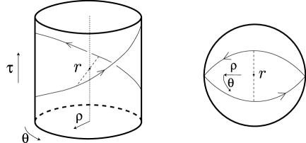
Figure 4: Collision of two particles in AdS. The trajectories are shown both in the full space $\tau,\rho,\theta$ as well as projected onto a spatial slice $\rho,\theta$. The full configuration has total energy $E$ and spin $J$, with the particles reaching a minimum geodesic distance $r$ given by $\tanh\left(r/2\right)=J/E$.

They reach a minimum relative geodesic distance $r=2\rho_{\min}$ given by

$$\tanh\left(\frac{r}{2}\right)=\frac{J}{E}~{},$$

thus justifying geometrically the definition (3.9).

4.1 Free Propagation

The four–point amplitude $\mathcal{A}$ can be described dually as gravitational interaction in AdS space. In particular, neglecting string corrections, we have the expansion

$$\mathcal{A}=\mathcal{A}_{0}+\mathcal{A}_{1}+\mathcal{A}_{2}+\cdots,$$

in powers of the coupling constant $G$. The above expansion starts with the contribution from the disconnected graph in figure 1$(a)$, which describes free propagation in AdS and is given by the product of two–point functions $\left\langle\mathcal{O}_{1}\left(\mathbf{p}_{1}\right)\mathcal{O}_{1}\left(\mathbf{p}_{3}\right)\right\rangle\left\langle\mathcal{O}_{2}\left(\mathbf{p}_{2}\right)\mathcal{O}_{2}\left(\mathbf{p}_{4}\right)\right\rangle$. Choosing appropriate normalization for the external operators $\mathcal{O}_{1}$, $\mathcal{O}_{2}$ we have that

$$\mathcal{A}_{0}=1~{}.$$

From the graph, it is intuitively clear that, in the T–channel, only the vacuum state with $h=\bar{h}=0$ contributes, as shown in figure 5$(a)$.

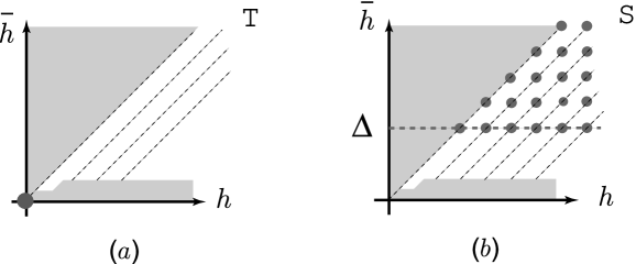
Figure 5: Partial wave decomposition of the amplitude $\mathcal{A}_{0}=1$ corresponding to free propagation in AdS in figure $1(a)$. In the T–channel decomposition only the vacuum contributes, whereas the S–channel decomposition receives contributions from a full lattice of $\mathcal{O}_{1}\mathcal{\partial}^{N}\mathcal{O}_{2}$ composites of dimensions $h,\bar{h}\in\Delta+\mathbb{N}_{0}$.

In fact, with an appropriate normalization for $\mathcal{T}_{h,\bar{h}}$ we have that

$$\mathcal{A}_{0}=\mathcal{T}_{0,0}~{}.$$ (4.18)

On the other hand, the S–channel decomposition of $\mathcal{A}_{0}$ is more subtle. In fact, as shown in figure 5$(b)$, we expect that the composites

$$\mathcal{O}_{1}\partial_{\mu_{1}}\cdots\partial_{\mu_{J}}\partial^{2n}\mathcal{O}_{2}\,,$$

of dimension $E=2\Delta+J+2n$ and spin $J$, contribute to the S–channel decomposition and define a lattice of operators of dimension $h=\Delta+J+n$, $\bar{h}=\Delta+n$ given by

$$h,\bar{h}\in\Delta+\mathbb{N}_{0}\text{ },~{}\ \ \ \ \ \ \ \ \ \ \ \ \ \ \ \ \ \ \ \Delta\leq\bar{h}\leq h~{}.$$

Again, with an appropriate normalization for the S–channel partial waves $\mathcal{S}_{h,\bar{h}}$, we have the decomposition

$$\mathcal{A}_{0}=\sum_{\Delta\leq\bar{h}\leq h}\ \mathcal{S}_{h,\bar{h}}~{},$$ (4.19)

where it is understood that the sum is restricted to $h,\bar{h}\in\Delta+\mathbb{N}_{0}$. Finally, we have the impact parameter representation corresponding to (4.19)

$$\mathcal{A}_{0}=\int_{0}^{\infty}dh\int_{0}^{h}d\bar{h}~{}~{}~{}\mathcal{I}_{h,\bar{h}}~{}.$$

Note that the normalizations chosen for the specific case $d=2$ are compatible with (4.18) and (4.19).

4.2 Tree–Level Interaction in the S–Channel

We expect that the full amplitude $\mathcal{A}$ can be expanded in S–channel partial waves as

$$\mathcal{A}\simeq\sum_{h\geq\bar{h}\geq\Delta}\left(1+R(h,\bar{h})\right)~{}\mathcal{S}_{h+\Gamma(h,\bar{h}),~{}\bar{h}+\Gamma(h,\bar{h})}~{}\ ,$$

where $2\Gamma(h,\bar{h})$ is the anomalous dimension of the intermediate primary and $R(h,\bar{h})$ is related to its three–point coupling to the external operators. We are assuming, by analogy with the flat space situation, that in the large $h$, $\bar{h}$ limit the relevant intermediate primaries are the composites $\mathcal{O}_{1}\partial^{N}\mathcal{O}_{2}$ that already contribute at leading order. Let us now analyze the tree–level graph $\mathcal{A}_{1}$ in figure 2$(a)$, corresponding to the exchange of a spin $j$ massless particle in AdS_d+1. Denoting by $\sigma_{h,\bar{h}}$ and $\rho_{h,\bar{h}}$ the contribution of this graph to $\Gamma(h,\bar{h})$ and $R(h,\bar{h})$, we can write

$$\mathcal{A}_{1}=\sum_{\Delta\leq\bar{h}\leq h}\ \sigma_{h,\bar{h}}\left(\frac{\partial}{\partial h}+\frac{\partial}{\partial\bar{h}}\right)\mathcal{S}_{h,\bar{h}}+\sum_{\Delta\leq\bar{h}\leq h}\ \rho_{h,\bar{h}}~{}\mathcal{S}_{h,\bar{h}}\ .$$ (4.20)

The tree–level eikonal computation of the graph 2$(a)$ does not give an approximation to the amplitude $\mathcal{A}_{1}$, as one would expect by analogy with the flat space result. Rather, as was shown in [6], it computes the small $z,\bar{z}$ behavior of the discontinuity function (or monodromy of the amplitude around the point at infinity)

$$\mathcal{M}_{1}\left(z,\bar{z}\right)=\operatorname{Disc}{}_{z}~{}\mathcal{A}_{1}\left(z,\bar{z}\right)\equiv\frac{1}{2\pi i}\left(\mathcal{A}_{1}^{\circlearrowright}\left(z,\bar{z}\right)-\mathcal{A}_{1}\left(z,\bar{z}\right)\right),$$

where $\mathcal{A}_{1}^{\circlearrowright}$ is the analytic continuation of $\mathcal{A}_{1}$ obtained by keeping $\bar{z}$ fixed and by transporting $z$ clockwise around the point at infinity as in figure 6.

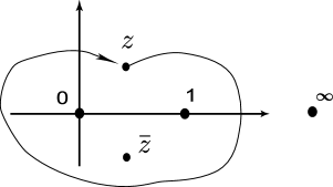
Figure 6: Analytic continuation of $\mathcal{A}_{1}$ to obtain $\mathcal{A}_{1}^{\circlearrowright}$. The variable $\bar{z}$ is kept fixed and $z$ is transported clockwise around the point at infinity, circling the points $0,1,\bar{z}$.

Since $\mathcal{S}_{h,\bar{h}}$ behaves around $z,\bar{z}\sim\infty$ as

$$z^{\Delta-h}\bar{z}^{\Delta-\bar{h}}\sum_{n,\bar{n}\geq 0}z^{-n}\bar{z}^{-\bar{n}}c_{n,\bar{n}}\left(h,\bar{h}\right)+\left(z\leftrightarrow\bar{z}\right)~{},$$

we have that, for $h,\bar{h}\in\Delta+\mathbb{N}_{0}$,

$$\left(\frac{\partial}{\partial h}+\frac{\partial}{\partial\bar{h}}\right)\mathcal{S}_{h,\bar{h}}=-\ln\left(z\bar{z}\right)\mathcal{S}_{h,\bar{h}}+\cdots~{},$$

where the terms in the dots have an expansion around $z,\bar{z}\sim\infty$ with integer powers of $z^{-1},\bar{z}^{-1}$ and do not contribute to $\mathcal{M}_{1}$. It is then clear that

$$\mathcal{M}_{1}\left(z,\bar{z}\right)=\sum_{\Delta\leq\bar{h}\leq h}\ \sigma_{h,\bar{h}}~{}\mathcal{S}_{h,\bar{h}}\left(z,\bar{z}\right)$$ (4.21)

carries all the information about the anomalous dimensions $\sigma_{h,\bar{h}}$.

In [6] it was shown that the leading behavior of $\mathcal{M}_{1}$ for small $z,\bar{z}$ is given by

$$\mathcal{M}_{1}\simeq -8G\mathcal{N}_{\Delta_{1}}\mathcal{N}_{\Delta_{2}}\Gamma\left(2\Delta_{1}-1+j\right)\Gamma\left(2\Delta_{2}-1+j\right)\times$$ (4.22)

$$\times~{}\left(-q^{2}\right)^{\Delta_{1}}\left(-p^{2}\right)^{\Delta_{2}}\int_{\mathrm{H}_{d-1}}\widetilde{dx}\widetilde{dy}~{}\frac{\Pi\left(x,y\right)}{\left(2q\cdot x\right)^{2\Delta_{1}-1+j}\left(2p\cdot y\right)^{2\Delta_{2}-1+j}}~{},$$

where $\Pi\left(x,y\right)$ is the Euclidean scalar propagator on the hyperbolic space $\mathrm{H}_{d-1}$ with mass squared $d-1$ given in (2.8). The leading behavior is then of the form

$$\mathcal{M}_{1}\left(z,\bar{z}\right)\simeq\left(-z\right)^{1-j}M\left(\frac{\bar{z}}{z}\right)~{},$$

with $M\left(w\right)^{\star}=M\left(w^{\star}\right)$ and $M\left(w\right)=w^{1-j}M\left(1/w\right)$. Recall from section 3.2 that, in the limit of small $z,\bar{z}$, we may approximate $\mathcal{M}_{1}$ with the impact parameter representation

$$\mathcal{M}_{1}\simeq\int dhd\bar{h}\ \sigma_{h,\bar{h}}~{}\mathcal{I}_{h,\bar{h}}~{},$$ (4.23)

where the leading behavior of $\sigma_{h,\bar{h}}$ for large $h,\bar{h}$ determines the leading behavior of $\mathcal{M}_{1}$ at small $z,\bar{z}$. To match (4.23) with (4.22) using the integral representation (3.17) it is convenient to express the integral over the hyperboloids in (4.22) as an integral over Milne wedges

$$\mathcal{M}_{1}\simeq -8G\mathcal{N}_{\Delta_{1}}\mathcal{N}_{\Delta_{2}}\left(-q^{2}\right)^{\Delta_{1}}\left(-p^{2}\right)^{\Delta_{2}}\times$$

$$\times~{}\int_{M}\,\frac{d(t_{1}\,x)}{t_{1}^{d-2\Delta_{1}-j+1}}\,\frac{d(t_{2}\,y)}{t_{2}^{d-2\Delta_{2}-j+1}}\,e^{-2q\cdot(t_{1}\,x)-2p\cdot(t_{2}\,y)}\,\Pi\left(x,y\right)\ .$$

We then conclude that the leading behavior of the anomalous dimensions $\sigma_{h,\bar{h}}$ for large $h,\bar{h}$ is given by

$$\sigma_{h,\bar{h}}\simeq-8G~{}\left(\frac{s}{4}\right)^{j-1}\Pi\left(x,y\right)~{},~{}\;\ \ \ \ \ \ \ \ \ \ \left(s\rightarrow\infty\right),$$ (4.24)

where $s=4h\bar{h}$. The propagator $\Pi\left(x,y\right)$ depends only on the geodesic distance $r$ between $x,y\in\mathrm{H}_{d-1}$, which is given by $\cosh r=-x\cdot y$ and it is related to the conformal dimensions by

$$e^{-r}=\frac{\bar{h}}{h}~{}.$$

Using the explicit form (2.8) of the propagator, we can express $\Pi$ in terms of the conformal dimensions $h,\bar{h}$ for various dimensions $d$, as shown in the following table:

$$d$$

The eikonal result (4.22) allowed us to determine, in the S–channel partial wave decomposition (4.20), the high spin and energy behavior of the anomalous dimensions $\sigma_{h,\bar{h}}$, but not of the coefficients $\rho_{h,\bar{h}}$. We will now show that in fact

$$\rho_{h,\bar{h}}\simeq\partial\sigma_{h,\bar{h}}$$ (4.25)

up to sub–leading terms, where we use the notation

$$\partial=\partial_{h}+\partial_{\bar{h}}\,.$$

In this case, the high $h,\bar{h}$ behavior of the amplitude $\mathcal{A}_{1}$ can be fully reconstructed from $\mathcal{M}_{1}$ and is given by

$$\mathcal{A}_{1}\simeq\sum_{h\geq\bar{h}\geq\Delta}\partial\left(\sigma_{h,\bar{h}}\mathcal{S}_{h,\bar{h}}\right)~{}.$$ (4.26)

In order to show this, consider the part of $\mathcal{A}_{1}$ which is of the form $\sum\sigma_{h,\bar{h}}\partial\mathcal{S}_{h,\bar{h}}$. It is approximated by $\int dhd\bar{h}~{}\left(\partial\sigma_{h,\bar{h}}\right)\mathcal{I}_{h,\bar{h}}$, where we have replaced $\sum\rightarrow\int$, $\mathcal{S}\rightarrow\mathcal{I}$ and where we have integrated by parts. The leading behavior of the above integral for $z,\bar{z}\rightarrow 0$ is $\left(z\bar{z}\right)^{\frac{3}{4}-\frac{j}{2}}$, since $\partial\sigma_{h,\bar{h}}\sim\left(h\bar{h}\right)^{j-\frac{3}{2}}$. On the other hand, the OPE expansion of $\mathcal{A}_{1}$ is dominated by the exchange of the massless particle and must start with $\left(z\bar{z}\right)^{\frac{d}{2}}$. Therefore, the term in $\mathcal{A}_{1}$ of the form $\sum\rho_{h,\bar{h}}\mathcal{S}_{h,\bar{h}}$ must compensate the anomalous dimension contribution, giving (4.26), which is a total derivative in the impact parameter approximation and which is therefore sub–leading near $z,\bar{z}\sim 0$.

4.3 Tree–Level Interaction in the T–Channel

The function $\mathcal{M}_{1}$ can also be used to obtain information regarding the decomposition of the tree–level graph $\mathcal{A}_{1}$ in T–channel partial waves. Decomposing the amplitude $\mathcal{A}_{1}$ as

$$\mathcal{A}_{1}=\sum\ \mu_{h,\bar{h}}~{}\mathcal{T}_{h,\bar{h}}~{},$$ (4.27)

the function $\mathcal{M}_{1}$ can be written as

$$\mathcal{M}_{1}=\sum\ \mu_{h,\bar{h}}\operatorname{Disc}{}_{z}~{}\mathcal{T}_{h,\bar{h}}~{}.$$

Thus, we must first analyze in detail the behavior of the functions $\mathcal{T}_{h,\bar{h}}\left(z,\bar{z}\right)$ as we rotate the point $z$ clockwise around infinity, keeping $\bar{z}$ fixed. Since the eikonal result (4.22) holds around $z,\bar{z}\sim 0$, we shall need only the leading behavior of $\operatorname{Disc}{}_{z}~{}\mathcal{T}_{h,\bar{h}}$ around the origin.

Consider first the behavior of $\mathcal{T}_{h,\bar{h}}$ in the limit $\bar{z}\rightarrow 0$, with $z$ fix. The operator $D_{T}$ in (3.10) reduces to

$$z^{2}\left(1-z\right)\partial^{2}-z^{2}\partial+\bar{z}^{2}\bar{\partial}^{2}-\left(d-2\right)\bar{z}\bar{\partial}~{}.$$

Using the boundary condition $\mathcal{T}_{h,\bar{h}}\sim\left(-z\right)^{h}\left(-\bar{z}\right)^{\bar{h}}$ around the origin, we conclude that

$$\mathcal{T}_{h,\bar{h}}\sim\left(-\bar{z}\right)^{\bar{h}}\left(-z\right)^{h}F\Big{(}h,h,2h\Big{|}z\Big{)}~{}.$$

Since

$$\left(-z\right)^{h}F\Big{(}h,h,2h\Big{|}z\Big{)} =\frac{\Gamma\left(2h\right)}{\Gamma\left(h\right)^{2}}\sum_{n\geq 0}\frac{\left(h\right)_{n}\left(1-h\right)_{n}}{\left(n!\right)^{2}}z^{-n}\times$$

$$\times\bigg{(}\ln\left(-z\right)+2\psi\left(n+1\right)-\psi\left(h+n\right)-\psi\left(h-n\right)\bigg{)}$$

we obtain that

$$\operatorname{Disc}{}_{z}~{}\mathcal{T}_{h,\bar{h}}\sim-\frac{\Gamma\left(2h\right)}{\Gamma\left(h\right)^{2}}\left(-\bar{z}\right)^{\bar{h}}F\Big{(}h,1-h,1\Big{|}z^{-1}\Big{)}~{}.$$

In the limit of small $z$ the leading behavior is

$$\operatorname{Disc}{}_{z}~{}\mathcal{T}_{h,\bar{h}}\sim-\frac{\Gamma\left(2h\right)\Gamma\left(2h-1\right)}{\Gamma\left(h\right)^{4}}~{}\left(-z\right)^{1-h}\left(-\bar{z}\right)^{\bar{h}}~{}.$$ (4.28)

Recall that we derived this result in the limit $\bar{z}\rightarrow 0$. To understand the general behavior around $z,\bar{z}\sim 0$ of $\operatorname{Disc}{}_{z}~{}\mathcal{T}_{h,\bar{h}}$, we expand $\mathcal{T}_{h,\bar{h}}$ in powers of $\bar{z}$ as

$$\mathcal{T}_{h,\bar{h}}\sim\sum_{n\geq 0}\left(-\bar{z}\right)^{\bar{h}+n}g_{n}\left(z\right)~{}.$$ (4.29)

We have just determined that $\operatorname{Disc}{}_{z}~{}g_{0}\sim z^{1-h}$ for small $z$. The other functions $g_{n}$ are determined recursively by expanding the differential equation $D_{T}=c_{h,\bar{h}}$ in powers of $\bar{z}$. A rather cumbersome but straightforward computation shows that $\operatorname{Disc}{}_{z}~{}g_{n}\sim z^{1-h-n}$ for small $z$. Therefore, we conclude in general that

$$\operatorname{Disc}{}_{z}~{}\mathcal{T}_{h,\bar{h}}\sim\left(-z\right)^{1-h}\left(-\bar{z}\right)^{\bar{h}}~{}G_{h,\bar{h}}\left(\frac{\bar{z}}{z}\right)$$ (4.30)

around $z,\bar{z}\sim 0$. The function $G_{h,\bar{h}}\left(w\right)$ is regular around $w=0$ and, using (4.28), satisfies $G_{h,\bar{h}}\left(0\right)=-\Gamma\left(2h\right)\Gamma\left(2h-1\right)/\Gamma\left(h\right)^{4}$. The careful reader will have noticed that in equation (4.29) we have implicitly neglected to symmetrize in $z\leftrightarrow\bar{z}$. Had we not, the function $\mathcal{T}_{h,\bar{h}}$ would have had an extra contribution of the form $\sum_{n\geq 0}\left(-\bar{z}\right)^{h+n}f_{n}\left(z\right)$ with $\operatorname{Disc}{}_{z}~{}f_{n}\sim z^{1-\bar{h}-n}$. These terms then give sub–leading contributions to (4.30).

To compute explicitly the function $G_{h,\bar{h}}$, we consider the operator $D_{T}$ in (3.10) near $z,\bar{z}\sim 0$, which reduces to

$$z^{2}\partial^{2}+\bar{z}^{2}\bar{\partial}^{2}+\left(d-2\right)\frac{z\bar{z}}{z-\bar{z}}\left(\partial-\bar{\partial}\right)~{}.$$

Acting on (4.30) the differential equation $D_{T}=c_{h,\bar{h}}$ becomes of the hypergeometric form

$$2w\left(1-w\right)G^{\prime\prime}+\left[2\left(h+\bar{h}\right)\left(1-w\right)-\left(d-2\right)\left(1+w\right)\right]G^{\prime}=\left(d-2\right)\left(h+\bar{h}-1\right)G~{},$$

in terms of $w=\bar{z}/z$. We then arrive at the result

$$G_{h,\bar{h}}=-\frac{\Gamma\left(2h\right)\Gamma\left(2h-1\right)}{\Gamma\left(h\right)^{4}}~{}F\left.\left(\frac{d}{2}-1,h+\bar{h}-1,h+\bar{h}+1-\frac{d}{2}\right|\frac{\bar{z}}{z}\right)~{}.$$ (4.31)

We are now in a position to determine the implications of the eikonal result (4.22) for the T–channel expansion coefficients $\mu_{h,\bar{h}}$ in (4.27).

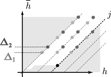
Figure 7: T–channel decomposition of the spin $j$ exchange graph in figure $2(a)$. Only partial waves with spin $J\leq j$ contribute. The eikonal integral determines the contributions with $J=j$, along the thick dashed line. We display with a black dot the contribution from the operator dual to the exchanged particle, with spin $j$ and energy $d-j$. We also show, with light and dark grey dots, the contributions from the $\mathcal{O}_{1}\partial^{N}\mathcal{O}_{1}$ and $\mathcal{O}_{2}\partial^{N}\mathcal{O}_{2}$ composites, with dimensions $h,\bar{h}\in\Delta_{1}+\mathbb{N}_{0}$ and $h,\bar{h}\in\Delta_{2}+\mathbb{N}_{0}$, respectively.

Recall that the leading behavior of $\mathcal{M}_{1}$ for small $z,\bar{z}$ is controlled by

$$\mathcal{M}_{1}\simeq\left(-z\right)^{1-j}M\left(\frac{\bar{z}}{z}\right),$$

as derived in the dual AdS description. We therefore immediately conclude from (4.30) that, in the decomposition (4.27), only partial waves with

$$J=h-\bar{h}\leq j$$

can appear, as shown in figure 7. Moreover, the coefficients $\mu_{h,\bar{h}}$ for $J=h-\bar{h}=j$ are determined directly by the function $M\left(w\right)$ from

$$\sum_{h-\bar{h}=j}\mu_{h,\bar{h}}~{}w^{\bar{h}}~{}G_{h,\bar{h}}\left(w\right)=M\left(w\right)~{}.$$ (4.32)

In the simple case of $d=2$ the functions $G_{h,\bar{h}}$ are constants, so that the coefficients $\mu_{h,\bar{h}}$ are simply obtained by expanding $M$ in increasing powers of $w$.

4.4 An Example in $d=2$

To be more explicit we conclude this section with a simple example where we can check our results. We shall consider the case $d=\Delta_{2}=2$ and $j=0$ corresponding to massless scalar exchange in AdS₃. As shown in [6], the basic amplitude $\mathcal{A}_{1}$ is given by

$$\mathcal{A}_{1}=\frac{8G}{\pi}~{}\mathbf{p}_{13}^{\Delta_{1}}\mathbf{p}_{24}~{}D_{\Delta_{1},\Delta_{1},1,1}^{2}\left(\mathbf{p}_{1},\mathbf{p}_{3},\mathbf{p}_{2},\mathbf{p}_{4}\right)~{}.$$ (4.33)

where $D^{d}_{\Delta_{i}}\left(\mathbf{p}_{i}\right)$ are the standard $D$–functions [11, 6]. On the other hand, in [6] we have also explicitly computed the integral (4.22), which controls the leading behavior of $\mathcal{M}_{1}=\operatorname*{Disc}_{z}\mathcal{A}_{1}$ as $z,\bar{z}\rightarrow 0$, obtaining $\mathcal{M}_{1}\simeq-zM\left(\bar{z}/{z}\right),$ with $M\left(w\right)$ given by

$$M\left(w\right)=-\frac{4G}{2\Delta_{1}-1}\,wF\Big{(}1,\Delta_{1},2\Delta_{1}\Big{|}1-w\Big{)}.$$ (4.34)

Recall, from the discussion in section 4.3, that the function $M\left(w\right)$ contains information about the T–channel expansion of $\mathcal{A}_{1}$

$$\mathcal{A}_{1}=\sum_{h}\mu_{h,h}~{}\mathcal{T}_{h,h}~{},$$

which has only spin zero contributions. More precisely, the expansion (4.32), with the explicit form of $G_{h,\bar{h}}$ in (4.31), becomes

$$M\left(w\right)=-\sum_{h}\mu_{h,h}~{}\frac{\Gamma\left(2h\right)\Gamma\left(2h-1\right)}{\Gamma\left(h\right)^{4}}w^{h}~{}.$$

Using the standard properties of the hypergeometric functions, we may expand $M\left(w\right)$ in (4.34) around $w=0$ as

$$M\left(w\right) =4G\frac{\Gamma\left(1-\Delta_{1}\right)}{\Gamma\left(\Delta_{1}\right)}\sum_{h\in 1+\mathbb{N}_{0}}\frac{\Gamma\left(\Delta_{1}-1+h\right)}{\Gamma\left(1-\Delta_{1}+h\right)}w^{h}-$$

$$-4G\frac{\Gamma\left(1-\Delta_{1}\right)}{\Gamma\left(\Delta_{1}\right)}\sum_{h\in\Delta_{1}+\mathbb{N}_{0}}\frac{\Gamma\left(\Delta_{1}-1+h\right)}{\Gamma\left(1-\Delta_{1}+h\right)}w^{h},$$

finally concluding that

$$\mathcal{A}_{1}=-\mu_{1}\mathcal{T}_{1,1}+\sum_{h\in\Delta_{1}+\mathbb{N}_{0}}\mu_{h}\mathcal{T}_{h,h}-\sum_{h\in\Delta_{2}+\mathbb{N}_{0}}\mu_{h}\mathcal{T}_{h,h}~{},$$

with

$$\mu_{h}=4G\frac{\Gamma\left(1-\Delta_{1}\right)}{\Gamma\left(\Delta_{1}\right)}\frac{\Gamma\left(\Delta_{1}-1+h\right)}{\Gamma\left(1-\Delta_{1}+h\right)}\frac{\Gamma\left(h\right)^{4}}{\Gamma\left(2h\right)\Gamma\left(2h-1\right)}~{}.$$

The contributions come from the operator dual to the exchanged particle, with spin $j=0$ and energy $2$, as well as from the $\mathcal{O}_{1}\partial^{N}\mathcal{O}_{1}$ and $\mathcal{O}_{2}\partial^{N}\mathcal{O}_{2}$ composites, with dimensions $h=\bar{h}\in\Delta_{1}+\mathbb{N}_{0}$ and $h=\bar{h}\in\Delta_{2}+\mathbb{N}_{0}$ respectively, as shown in figures 7 and 8.

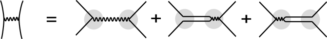
Figure 8: T–channel decomposition of the graph in figure $2(a)$. The contributions come from the operator dual to the exchanged particle as well as from the $\mathcal{O}_{1}\partial^{N}\mathcal{O}_{1}$ and $\mathcal{O}_{2}\partial^{N}\mathcal{O}_{2}$ composites.

Finally let us consider the expansion of $\mathcal{A}_{1}\,$ in the $S$–channel. We shall restrict further our attention to the special case of $\Delta_{1}=2$, where the amplitude (4.33) can be explicitly computed [12]

$$\mathcal{A}_{1}\left(z,\bar{z}\right)=-8G\frac{z^{2}\bar{z}^{2}}{\left(\bar{z}-z\right)}\left[\frac{1}{1-\bar{z}}\partial-\frac{1}{1-z}\bar{\partial}\right]a\left(z,\bar{z}\right)~{},$$

where

$$a\left(z,\bar{z}\right)=\frac{\left(1-z\right)\left(1-\bar{z}\right)}{\left(z-\bar{z}\right)}\left[\mathrm{Li}_{2}\left(z\right)-\mathrm{Li}_{2}\left(\bar{z}\right)+\frac{1}{2}\mathrm{\ln}\left(z\bar{z}\right)\mathrm{\ln}\left(\frac{1-z}{1-\bar{z}}\right)\right]~{},$$

with $\mathrm{Li}_{2}$ the dilogarithm. Using a symbolic manipulation program we can check the decomposition (4.20) up to very high order, with

$$\sigma_{h,\bar{h}} =-\frac{4G}{h\left(h-1\right)}~{},$$

$$\rho_{h,\bar{h}} =\left(\frac{\partial}{\partial h}+\frac{\partial}{\partial\bar{h}}\right)\sigma_{h,\bar{h}}+\frac{4G}{h\left(h-1\right)\bar{h}\left(\bar{h}-1\right)}~{}.$$

In the limit of large dimensions  $h$,$\bar{h}\rightarrow\infty$, we have $\sigma_{h,\bar{h}}\sim-4G/h^{2}$, as predicted from the general formula (4.24). In the same limit, we have $\rho_{h,\bar{h}}\simeq\partial\sigma_{h,\bar{h}}$, in agreement with (4.25).

5 Graviton Dominance

We have analyzed in great detail the tree–level exchange of a spin $j$ particle in the T–channel, given by graph 2$(a)$ in the introduction. We have noticed that, decomposing this graph in the S–channel and considering its contribution to partial waves of large spin and energy, the dominant amplitude has the maximal value for the spin $j$ of the exchanged particle. In gravitational theories in AdS, this particle is the graviton, whose exchange dominates the interaction and determines the tree–level anomalous dimensions of the double trace $\mathcal{O}_{1}\mathcal{O}_{2}$ composites to be $2\sigma_{h,\bar{h}}\simeq-4Gs\Pi\left(x,y\right)$ for large $h,\bar{h}$. On the other hand, the full gravitational theory in AdS will have more interactions at tree–level, like $S$ and $U$–channel exchanges, as well as contact and non–minimal interactions. Just as in flat space, though, all these other interactions are subdominant in the large spin and energy limit, and can be neglected in first approximation. We will not give a complete proof of this fact, but we shall rather concentrate on some specific significant examples. In particular, we will analyze the graphs already considered in the introduction (in figure 2), and we will concentrate on the case $\Delta_{1}=\Delta_{2}$ for simplicity.

Letting $\mathcal{A}_{1}(z,\bar{z})$ be the amplitude for graph 2$(a)$, the amplitudes for graphs 2$(b)$ and 2$(c)$ are simply obtained by permuting the external particles and are given explicitly by

$$\left(z\bar{z}\right)^{\Delta}\mathcal{A}_{1}\left(\frac{1}{z},\frac{1}{\bar{z}}\right),\text{ \ \ \ \ \ \ \ \ \ \ \ \ \ \ \ \ \ \ \ \ \ \ \ \ \ } \text{(graph }2(b)\text{)},$$

$$\left(\frac{z\bar{z}}{\left(1-z\right)\left(1-\bar{z}\right)}\right)^{\Delta}\mathcal{A}_{1}\left(1-z,1-\bar{z}\right),\text{ \ \ \ \ \ \ \ \ \ \ \ \ \ \ \ \ \ \ \ \ \ } \text{(graph }2(c)\text{)}.$$

The $S$–channel decomposition of graph 2$(b)$ can be trivially deduced from the results of section (4.3), which considers the mirror $T$–channel decomposition of graph 2$(a)$. Without any further analysis, we conclude that 2$(b)$ contributes only to $S$–channel partial waves of spin $J\leq j$, and is therefore local in spin as in flat space. It is therefore irrelevant when considering large spin and energy decomposition of the full tree–level amplitude.

To analyze the $S$–channel decomposition of graph 2$(c)$, let us first note that the differential operator $D_{S}$ in (3.11) is invariant under $z\rightarrow 1-z$ and $\bar{z}\rightarrow 1-\bar{z}$, whenever $2\nu=\Delta_{1}-\Delta_{2}=0$. We therefore conclude that

$$\left(\frac{z\bar{z}}{\left(1-z\right)\left(1-\bar{z}\right)}\right)^{\Delta}\mathcal{S}_{h,\bar{h}}\left(1-z,1-\bar{z}\right)=\left(-\right)^{h-\bar{h}}\mathcal{S}_{h,\bar{h}}\left(z,\bar{z}\right)~{},$$

where the normalization is fixed by recalling the leading behavior of $\mathcal{S}_{h,\bar{h}}\sim z^{\Delta-h}\bar{z}^{\Delta-\bar{h}}$ when $z,\bar{z}\rightarrow\infty$. In fact, if we choose $z=i\lambda$, $\bar{z}=-i\lambda$ to avoid branch cuts on the real axis, we have that $\mathcal{S}_{h,\bar{h}}\left(z,\bar{z}\right)\sim\left(i\lambda\right)^{\Delta-h}\left(-i\lambda\right)^{\Delta-\bar{h}}$ and that $\mathcal{S}_{h,\bar{h}}\left(1-z,1-\bar{z}\right)\sim\left(-i\lambda\right)^{\Delta-h}\left(i\lambda\right)^{\Delta-\bar{h}}$, thus fixing the relative normalization to $\left(-\right)^{h-\bar{h}}$. We then conclude that, if the $S$–channel expansion of $\mathcal{A}_{1}$ is given by (4.20), then graph 2$(c)$ is given by

$$\sum_{\Delta\leq\bar{h}\leq h}\ \left(-\right)^{h-\bar{h}}~{}\sigma_{h,\bar{h}}\left(\frac{\partial}{\partial h}+\frac{\partial}{\partial\bar{h}}\right)\mathcal{S}_{h,\bar{h}}+\sum_{\Delta\leq\bar{h}\leq h}\left(-\right)^{h-\bar{h}}\ \rho_{h,\bar{h}}~{}\mathcal{S}_{h,\bar{h}}~{}.$$

Therefore, for instance, the extra contribution to the anomalous dimension is given by

$$\left(-\right)^{h-\bar{h}}~{}2\sigma_{h,\bar{h}}~{},$$

which oscillates as a function of spin. In a coarse–grained picture in which we consider large impact parameters and continuous spins, these oscillations average to a vanishing function, just as in the flat space case considered in the introduction.

Finally, let us analyze the contact interaction of graph 2$(d)$. Using the techniques developed in [6], one can easily establish that the discontinuity $\operatorname*{Disc}{}_{z}$ of the amplitude corresponding to graph 2$(d)$ is proportional to

$$\left(-q^{2}\right)^{\Delta}\left(-p^{2}\right)^{\Delta}\int_{\mathrm{H}_{d-1}}\widetilde{dx}~{}\frac{1}{\left(2q\cdot x\right)^{2\Delta-1}\left(2p\cdot x\right)^{2\Delta-1}}~{}.$$ (5.35)

This expression is essentially equation (4.22) with $j=0$ and the propagator $\Pi\left(x,y\right)$ replaced by the delta function $\delta\left(x,y\right)$ on the transverse space $\mathrm{H}_{d-1}$. It is therefore easy to follow section 4 and interpret it in the S and in the T–channel partial wave expansions. On one hand, the discontinuity function is an impact parameter approximation to the high spin and energy anomalous dimensions, which are now proportional to

$$\frac{1}{s}\delta\left(x,y\right)~{},$$

where we recall that $s=4h\bar{h}$ and $-2x\cdot y=\bar{h}/h+h/\bar{h}$. Therefore the delta function fixes $h=\bar{h}$, i.e., spin $J=0$. On the other hand, since the discontinuity function (5.35) goes like $z$ for small $z,\bar{z}$, we have only spin $J=0$ partial waves appearing in the T–channel decomposition. Expression (5.35) also generates the relative weights of all these spin zero contributions. In both channels, as expected, graph 2$(d)$ only contains spin zero intermediate primaries, and therefore does not effect the large spin results which are only controlled by graph 2$(a)$.

6 A Conjecture and Conclusions

To complete the eikonal program, one crucial step is missing. In flat space, one can approximately reconstruct the full amplitude from the phase shift $\sigma$ using (1.3). This step cannot be immediately done in $\mathrm{AdS}_{d+1}$, even at tree–level, since the eikonal two–point function computed in [6] determines only the leading behavior of the discontinuity $\mathcal{M}_{1}$ of the relevant tree–level amplitude $\mathcal{A}_{1}$ in figure 2a. Nevertheless, we can be bold and try to reconstruct the full amplitude $\mathcal{A}$ from $\sigma_{h,\bar{h}}$. We shall assume that $\mathcal{A}$ is dominated at large $h,\bar{h}$ only by the $\mathcal{O}_{1}\mathcal{O}_{2}$ composites with finite anomalous dimensions $\Gamma(h,\bar{h})$. This implies a decomposition of the form

$$\mathcal{A}\simeq\sum_{h\geq\bar{h}\geq\Delta}\left(1+R(h,\bar{h})\right)~{}\mathcal{S}_{h+\Gamma(h,\bar{h}),~{}\bar{h}+\Gamma(h,\bar{h})}~{}\ ,$$ (6.36)

where $R(h,\bar{h})$ are now finite coefficients. Expanding in powers of $\Gamma$ and dropping the explicit reference to $h,\bar{h}$, the above equation reads

$$\mathcal{A}\simeq\sum~{}\left(1+R\right)\left(1+\Gamma\partial+\frac{1}{2}\Gamma^{2}\partial^{2}+\cdots\right)~{}\mathcal{S}\text{~{}}.$$

The coefficients $R=R_{1}+R_{2}+\cdots$ and the anomalous dimensions $\Gamma=\Gamma_{1}+\Gamma_{2}+\cdots$ are computed in perturbation theory, with $\Gamma_{1}\simeq\sigma$ and $R_{1}\simeq\partial\sigma$. Order by order in the loop expansion, we then have the following expansions

$$\mathcal{A}_{0} \simeq\sum~{}\mathcal{S}~{},$$

$$\mathcal{A}_{1} \simeq\sum~{}R_{1}\,\mathcal{S}+\Gamma_{1}\,\partial\mathcal{S}~{},$$

$$\mathcal{A}_{2} \simeq\sum~{}R_{2}\,\mathcal{S}+\left(\Gamma_{2}+R_{1}\Gamma_{1}\right)\,\partial\mathcal{S+}\frac{1}{2}\Gamma_{1}^{2}\,\partial^{2}\mathcal{S}~{},$$

$$\cdots$$

Since $\Gamma_{1}\simeq\sigma$, it is tempting to assume, in analogy with (4.26), that in general

$$\mathcal{A}_{n}\simeq\frac{1}{n!}\sum~{}\partial^{n}\,\left(\sigma^{n}\mathcal{S}\right)~{}.$$

This is compatible with (6.36) provided that

$$\Gamma\simeq\sum_{n\geq 1}\frac{1}{n!}\partial^{n-1}\sigma^{n}~{},~{}\ \ \ \ \ \ \ \ \ \ \ \ \ \ \ R=\partial\Gamma~{}.\,$$

For example, consider graviton exchange in $d=2$, where $\sigma\simeq-4G\bar{h}^{2}$. The sum over $n$ can be done explicitly, arriving at the following intriguing formula for the anomalous dimension

$$\Gamma\simeq\frac{2\bar{h}}{1+\sqrt{1+16G\bar{h}}}-\bar{h}\ ,\ \ \ \ \ \ \ \ \ \ \ \ \ \ \ \ \ \ \ \ \ \ \ \ \ \ \ \ \left(j=2,~{}d=2\right).$$

Clearly the results above are purely conjectural, and we must leave a complete discussion of these issues for future research.

Finally, it would be very interesting to apply the techniques developed in this paper to specific realizations of the AdS/CFT correspondence. All of our discussion has been carried out for pure AdS, decomposing the amplitudes in conformal partial waves related to the isometries $SO\left(2,d\right)$ of the underlying spacetime. The impact parameter representation has also been derived accordingly. It is thus important to generalize the discussion to AdS $\times$ compact spaces and to superspaces, with partial waves and impact parameter representations appropriate for the isometry group of the full (super)space, including internal (and possibly super) symmetries. This could then allow us to test our results against computations performed directly in CFT duals at finite $N$.

Even though all computations in this paper are done in the gravity regime, neglecting string effects, it known [13] that, in some cases, string effects do not alter the general eikonal results in flat space. It is therefore tempting to speculate that some of the results of this paper could be already visible in weakly coupled CFT’s at finite $N$.

Appendix A Impact Parameter Representation

In this appendix we show that the integral representation (3.16) of the impact parameter representation partial wave $\mathcal{I}_{h,\bar{h}}$ solves the differential equation (3.15). We start by recalling the relevant kinematics. Choosing the four external points $\mathbf{p}_{i}$ as

$$\mathbf{p}_{1} =\left(0,1,0\right)~{},\ \ \ \ \ \ \ \ \ \ \ \ \ \ \ \ \ \ \ \ \ \ \ \mathbf{p}_{2}=-\left(1,p^{2},p\right)~{},$$

$$\mathbf{p}_{3} =-\left(q^{2},1,q\right)~{},\ \ \ \ \ \ \ \ \ \ \ \ \ \ \ \ \ \ \ \mathbf{p}_{4}=\left(1,0,0\right)~{},$$

the cross ratios $z,\bar{z}$ are determined by

$$z\bar{z}=q^{2}p^{2},~{}\ \ \ \ \ \ \ \ \ \ \ \ \ \ \ \ z+\bar{z}=2p\cdot q~{}.$$

In what follows, we choose once and for all a fixed point $p\in-\mathrm{H}_{d-1}$, so that $p^{2}=-1$. We then view the S–channel impact parameter amplitude $\mathcal{I}_{h,\bar{h}}$ as a function just of $q$. Recall that, in terms of $z,\bar{z}$, the function $\left(z\bar{z}\right)^{-\Delta}\mathcal{I}_{h,\bar{h}}$ satisfies the following differential equation

$$z\partial^{2}+\bar{z}\bar{\partial}^{2}+\partial+\bar{\partial}+\frac{d-2}{z-\bar{z}}\left(z\partial-\bar{z}\bar{\partial}\right)=\frac{\nu^{2}}{z}+\frac{\nu^{2}}{\bar{z}}-h^{2}-\bar{h}^{2}.$$

A tedious computation shows that, in terms of $q$, the above equation can be written as

$$\left(q^{i}p^{j}-\frac{1}{2}\eta^{ij}q\cdot p\right)\frac{\partial}{\partial q^{i}}\frac{\partial}{\partial q^{j}}+\frac{d}{2}p^{i}\frac{\partial}{\partial q^{i}}=\nu^{2}\frac{2p\cdot q}{q^{2}}+h^{2}+\bar{h}^{2}~{}.$$ (A.37)

Consider first the following function

$$f\left(x\right)=\left|x\right|^{d}\int_{\mathrm{M}}dy~{}~{}e^{-2p\cdot y}~{}\delta\left(2y\cdot x~{}+h^{2}+\bar{h}^{2}\right)~{}\delta\left(x^{2}y^{2}-h^{2}\bar{h}^{2}\right)~{},$$

where we integrate over the future Milne cone $\mathrm{M}\in\mathbb{M}^{d}$ given by $y^{2}\leq 0,~{}y^{0}\geq 0$. Changing integration variable to

$$z=-x\frac{\left(x\cdot y\right)\left(x\cdot p\right)-x^{2}\left(y\cdot p\right)}{\left(x\cdot p\right)^{2}+x^{2}}+px^{2}\frac{\left(x\cdot p\right)\left(y\cdot p\right)+\left(y\cdot x\right)}{\left(x\cdot p\right)^{2}+x^{2}},$$

with $z^{2}=-x^{2}y^{2}$, $z\cdot p=-y\cdot x$, $z\cdot x=-x^{2}p\cdot y$ and $dz=\left|x\right|^{d}dy$, we also have the integral representation

$$f\left(x\right)=\int_{\mathrm{M}}dz~{}~{}e^{-\frac{2x\cdot z}{x^{2}}}~{}\delta\left(2z\cdot p~{}-h^{2}-\bar{h}^{2}\right)~{}\delta\left(z^{2}+h^{2}\bar{h}^{2}\right)~{},$$

from which it is clear that the function $f\left(x\right)$ satisfies

$$~{}p^{i}\frac{\partial}{\partial\left(x^{i}/x^{2}\right)}f=\left(x^{2}p^{j}-2p\cdot x~{}x^{j}\right)\frac{\partial}{\partial x^{j}}f=-\left(h^{2}+\bar{h}^{2}\right)~{}f~{}.$$ (A.38)

We now consider the following function

$$g\left(q\right)=\left(-q^{2}\right)^{\nu}\int_{\mathrm{M}}\frac{dx}{\left|x\right|^{d-4\nu}}~{}e^{-2q\cdot x}~{}f\left(x\right)~{}.$$ (A.39)

We claim that $g\left(q\right)$ satisfies the differential equation (A.37). Replacing

$$\frac{\partial}{\partial q^{i}} \rightarrow 2\left(\nu\frac{q_{i}}{q^{2}}-x_{i}\right),$$

$$\frac{\partial}{\partial q^{i}}\frac{\partial}{\partial q^{j}} \rightarrow 2\nu\left(\frac{\eta_{ij}}{q^{2}}-2\frac{q_{i}q_{j}}{q^{4}}\right)+4\left(\nu\frac{q_{i}}{q^{2}}-x_{i}\right)\left(\nu\frac{q_{j}}{q^{2}}-x_{j}\right),$$

one can easily show that (A.37) is equivalent to

$$\left(-q^{2}\right)^{\nu}\int_{\mathrm{M}}\frac{dx}{\left|x\right|^{d-4\nu}}~{}e^{-2q\cdot x}~{}\left[4\left(q\cdot x\right)\left(p\cdot x\right)-2x^{2}\left(q\cdot p\right)-\right.$$

$$\left.-\left(d+4\nu\right)\left(p\cdot x\right)-h^{2}-\bar{h}^{2}\right]~{}f\left(x\right)=0~{}.$$

Using (A.38) the above is equivalent to

$$\left(-q^{2}\right)^{\nu}\int_{\mathrm{M}}\frac{dx}{\left|x\right|^{d-4\nu}}~{}e^{-2q\cdot x}~{}\left[4\left(q\cdot x\right)\left(p\cdot x\right)-2x^{2}\left(q\cdot p\right)-\right.$$

$$\left.-\left(d+4\nu\right)\left(p\cdot x\right)+\left(x^{2}p^{j}-2p\cdot x~{}x^{j}\right)\frac{\partial}{\partial x^{j}}\right]~{}f\left(x\right)=0~{},$$

which in turn is equal to

$$\int_{\mathrm{M}}dx~{}\frac{\partial}{\partial x^{j}}\left[\left(-x^{2}\right)^{-\frac{d}{2}+2\nu}\left(x^{2}p^{j}-2p\cdot x~{}x^{j}\right)e^{-2q\cdot x}~{}f\left(x\right)\right]=0~{}.$$

This last equation is true since the boundary value on $\partial\mathrm{M}$, of the term in the square brackets, vanishes.

We have therefore proved that $\left(-q^{2}\right)^{-\Delta}\mathcal{I}_{h,\bar{h}}\propto g$. Choosing a convenient normalization and going back to a general choice of $p$ we have arrived at the result (3.16).

References

- [1] J. M. Maldacena, The Large Limit of Superconformal Field Theories and Supergravity, Adv. Theor. Math. Phys. 2 (1998) 231, [arXiv:hep-th/9711200].
- [2] S. S. Gubser, I. R. Klebanov and A. M. Polyakov, Gauge Theory Correlators from Non–Critical String Theory, Phys. Lett. B428 (1998) 105, [arXiv:hep-th/9802109].
- [3] E. Witten, Anti–de Sitter Space and Holography, Adv. Theor. Math. Phys. 2 (1998) 253, [arXiv:hep-th/9802150].
- [4] D. Z. Freedman, S. D. Mathur, A. Matusis and L. Rastelli, Correlation Functions in the CFTd/AdSd+1 Correspondence, Nucl. Phys. B546 (1999) 96, [arXiv:hep-th/9804058].
- [5] O. Aharony, S. S. Gubser, J. M. Maldacena, H. Ooguri and Y. Oz, Large N Field Theories, String Theory and Gravity, Phys. Rept. 323 (2000) 183, [arXiv:hep-th/9905111].
- [6] L. Cornalba, M. S. Costa, J. Penedones and R. Schiappa, Eikonal Approximation in AdS/CFT: From Shock Waves to Four–Point Functions, [arXiv:hep-th/0611122].
- [7] E. D’Hoker, D. Z. Freedman, S. D. Mathur, A. Matusis and L. Rastelli, Graviton Exchange and Complete 4–Point Functions in the AdS/CFT Correspondence, Nucl. Phys. B562 (1999) 353, [arXiv:hep-th/9903196].
- [8] E. D’Hoker, S. D. Mathur, A. Matusis and L. Rastelli, The Operator Product Expansion of SYM and the 4–Point Functions of Supergravity, Nucl. Phys. B589 (2000) 38, [arXiv:hep-th/9911222].
- [9] F. A. Dolan and H. Osborn, Conformal Partial Waves and the Operator Product Expansion, Nucl. Phys. B678 (2004) 491, [arXiv:hep-th/0309180].
- [10] F. A. Dolan and H. Osborn, Conformal Four–Point Functions and the Operator Product Expansion, Nucl. Phys. B599 (2001) 459, [arXiv:hep-th/0011040].
- [11] E. D’Hoker and D. Z. Freedman, Supersymmetric Gauge Theories and the AdS/CFT Correspondence, [arXiv:hep-th/0201253].
- [12] M. Bianchi, M. B. Green, S. Kovacs and G. Rossi, Instantons in Supersymmetric Yang–Mills and D–Instantons in IIB Superstring Theory, JHEP 9808 (1998) 013, [arXiv:hep-th/9807033].
- [13] D. Amati, M. Ciafaloni and G. Veneziano, Superstring Collisions at Planckian Energies, Phys. Lett. B197 (1987) 81.