Making a Universe

Abstract

For understanding the origin of anisotropies in the cosmic microwave background, rules to construct a quantized universe is proposed based on the dynamical triangulation method of the simplicial quantum gravity. A $d$-dimensional universe having the topology $D^{d}$ is created numerically in terms of a simplicial manifold with $d$-simplices as the building blocks. The space coordinates of a universe are identified on the boundary surface $S^{d-1}$, and the time coordinate is defined along the direction perpendicular to $S^{d-1}$. Numerical simulations are made mainly for 2-dimensional universes, and analyzed to examine appropriateness of the construction rules by comparing to analytic results of the matrix model and the Liouville theory. Furthermore, a simulation in 4-dimension is made, and the result suggests an ability to analyze the observations on anisotropies by comparing to the scalar curvature correlation of a $S^{2}$-surface formed as the last scattering surface in the $S^{3}$ universe.

1 Introduction

Recent observations of anisotropies in the cosmic microwave background (CMB) by COBE and WMAP [1, 2, 3] extend our knowledge on the history of the universe beyond the big bang. They imply as follows: about 14 billion years ago, the universe started expanding with extremely rapid acceleration, now known as inflation [4, 5], from a micro-universe of quantum mechanical scale. Because of the expansion speed exceeding the light velocity, the pattern of original quantum fluctuations in space could not be disturbed dynamically, and was kept intact during the expansion something like a picture printed on an inflating balloon. After a little while($10^{-33}\sim 10^{-32}$ sec) the expansion was slowed down through coupling to matter fields, and fluctuations developed in the space curvature transferred to matter density fluctuations. They eventually are observed as the temperature anisotropies in the CMB, caused by the photon energy dissipation in fluctuating media known as the Sachs-Wolfe mechanism [6].

Although the observed data are rather well-understood by known physical processes with several phenomenological parameters, questions such as how and what kind of fluctuations were created initially, and why the universe could expand so rapidly are left to be the matters which essentially belong to the fundamental lows of space-time. In the history of studies on quantum gravity it is the most remarkable occasion where the theory is required to be phenomenological, apart from describing quantum fluctuation of geometry, the graviton, whose appearance is beyond the current experimental scope. It is a common belief that there exists no consistent theory that combines quantum mechanics and gravity at the moment. Among various efforts to establish quantum theory of gravity the super-string is regarded to be the most promising candidate as far as quantization of the graviton is concerned. It is extraordinary that the superstring theory can unify all the known interactions on the way of quantizing graviton. However, it does not say much about how the space-time is created. While absence of a consistent theory of quantum gravity is true in 4-dimension, we certainly have consistent theories of quantum gravity at least in 2-dimension. One of them is a standard field theory called the Liouville field theory [7], and the other is the matrix model [8]. In addition, the latter model has a numerical realization known as the dynamical triangulation (DT) [9].

The existence of analytic theories is closely tied to the dimensionality of space, and it is not a straightforward task at all to extend those theories into higher dimensions. The conformal gravity [10, 11] is one of possible generalizations of the Liouville theory into 4-dimension. It is free from space singularities such as the black hole of quantum mechanical size, and claimed to be renormalizable. However, it is unfortunate that the non-unitary nature inherited in any higher derivative field theory masks charms of the theory[12]. An extension of the discretized space model into higher dimensions beyond the matrix model has been proposed for the 3-dimensional space by adopting the $6j$-symbols as the elementary unit of space [13]. In an analogous manner it may be possible to extend further to the 4-dimensional space by introducing an appropriate elementary unit[14]. The simplicial quantum gravity is one of the constructive generalizations in the discretized space approach, selecting a $d$-simplex as the elementary block of the $d$-dimensional space. Numerical simulations have been performed for the $2,3,$ and $4$-dimensional simplicial spaces[15], and the grand canonical Monte Carlo simulations have produced significant results not only for the 2-dimensional case [16], but also for 4-dimension [17] in calculations of the string susceptibility which plays the role of a universal observable of the space geometry. As far as the possibility of extending the method into 4-dimension is concerned the simplicial quantum gravity is one of the promising cases so far exhibiting its applicability.

In modern field theories, quantization is often carried out by the Feynman path integral in which the Euclidean metric is adopted for definiteness of integrations. For a system having the stable vacuum it is always possible to transform the metric from the Euclidean to the Lorentzian and vice versa, by picking up one coordinate, which is regarded as the time coordinate, and making the Wick rotation. However, this procedure cannot be applied for a system without the stable vacuum. Quantum gravity is one of the systems having non-stationary vacuum of expanding space. Even though there exists no standard method of quantizing such a system, we employ the path integral method as a possibility to a space with open topology. While our final goal is to establish a method to construct the quantized universe in the 4-dimensional space-time, the following discussions are mainly proceeded on two dimensional space concerning the difficult circumstance of knowing no guiding theory. Besides its simplicity, analytic studies compiled extensively in 2-dimension are inevitable for achieving some hints required in this totally new subject. We would like to stress, however, that the constructive nature of the method will make it readily applicable to higher dimensional cases as well.

In the next section, we review the DT method mostly concentrating on the 2-dimensional space with the $S^{2}$ topology, and show that it provides a natural extension to a system with the open topology $D^{3}$. In Sec. 3, we shall practice to build an ensemble of 2-dimensional quantum universes based on two fundamental rules. In order to check the construction method we calculate observables of the space for systems with the stable vacua, by tuning the cosmological constant so that we can compare them to analytical results of the matrix model and the boundary Liouville theory [18]. In Sec. 4 we define the time and space coordinates of fluctuating manifold, and calculate the two point correlation function for the expanding universe. In the last section we give a summary and discussions on future directions such as a method extending into 4-dimension and problems related to the introduction of matter contents of the universe. There, we show a numerical result of the simulation in 4-dimension, which clearly indicates the applicability of the present method to the CMB anisotropies.

2 Methods of simplicial quantum gravity and their extension

The dynamical triangulation (DT) has been a standard method of non-perturbative quantum gravity [19] known as the simplicial quantum gravity. It was intensively studied in 2-dimension mainly because of its close connection to the string theory. Although we cannot expect new results from the 2-dimensional DT more than those already known from the matrix model and the Liouville theory, the achieved consistent results encourage us to adopt this method as a reliable technique for investigations beyond 2-dimension[12]. One of the drawbacks of the simplicial quantum gravity used to be the restriction to spaces with closed topologies with the Euclidean metric. In the followings, we would like to show how to extend the $d$-dimensional DT technique to a space with the open topology $D^{d}$ for $d\geq 2$. Besides the space-time topology the dynamics requires a proper signature of the metric, which is known to be Lorentzian in this universe. We regard the selection of the signature should come out naturally when we consider dynamics, since the correct signature, which is required by dynamical laws, supposed to emerge in the process of establishing the space-time.

Quantum gravity is formally defined in a form of the path integral,

$$Z=\int{\cal D}[g_{ab}]\exp(-S[g_{ab}]).$$ (1)

Here, we consider the simplest case that the metric tensor $g_{ab}$ is the unique dynamical variable. The space is assumed to have the dimension $d$ and the topology $S^{d}$ unless specified. The simplicial quantum gravity interprets the path integral to be a sum over all the distinct configurations of space discretized by $d$-simplices. For a $d$-dimensional manifold the action $S[g_{ab}]$ is given by a linear combination of the variables, $\{N_{n}\}$ with $n=0\cdots d$. It is considered to be natural, since we regard the diffeomorphysm invariance as its independence of the local geometry, or in other words, local variables. Thus only global variables such as the total number of $n$-simplices $N_{n}$ are proper, and linearity comes from the extensive property of the action function. The $(d+1)$ variables $\{N_{n}\}$ are not all independent. The Euler relationship and the manifold conditions reduce the number of independent variables. For example in 2-dimension, they are $N_{0}-N_{1}+N_{2}=\chi$ with $\chi$ being the Euler characteristic, and $3N_{2}=2N_{1}$. This makes the action to be $S^{(2)}=\mu N_{2}$ with a parameter$\mu$, which we call the lattice cosmological constant.

The set of distinct triangulations is collected computationally by the Metropolis Monte Carlo method creating a Markov chain of configurations $\{\alpha_{i}\}$,

$$\alpha_{0}\rightarrow\cdots\rightarrow\alpha_{i}\rightarrow\alpha_{i+1}\rightarrow\cdots.$$ (2)

Among possible methods of generating configurations one after another, we employ the so-called $(p,q)$-moves which allow us a systematic extension into higher dimensions. These moves are known to conserve the topology. There are three types of $(p,q)$-moves in 2-dimension as shown in Fig. 1. From the figures it is clear that $p$ and $q$ stand for the numbers of triangles disappeared and appeared by the $(p,q)$-move, respectively.

Figure 1: $(p,q)$-moves in the 2-dimensional simplicial gravity.

The Metropolis Monte Carlo method employs the importance sampling, accepting or non-accepting a new configuration created from an old configuration by a randomly selected move according to the detailed balance condition,

$$\frac{p_{\alpha}}{n_{\alpha}}w_{\alpha\rightarrow\beta}=\frac{p_{\beta}}{n_{\beta}}w_{\beta\rightarrow\alpha},$$ (3)

with the given probability $p_{\alpha}$ for a configuration $\alpha$. The factor $n_{\alpha}$ counts the number of possible moves starting from a configuration $\alpha$. This is an important factor for simulations with varying the number of the degree of freedom in order to obtain the proper statistical weight for each configuration.

The number of distinct triangulations is known to grow exponentially in $N_{2}$ for 2-dimension, and the partition function behaves as

$$Z\sim N_{2}^{\gamma-3}\exp\left\{-(\mu-\mu_{c})N_{2}\right\},$$ (4)

where $\gamma$ is historically called the string susceptibility. As $\mu$ approaches to a critical value $\mu_{c}$ from above, the average value of $N_{2}$ tends to diverge as $(\mu-\mu_{c})^{-1}$, and the system reaches to the continuum limit where the simulation meets the Liouville field theory with the field theoretical cosmological constant,

$$\lambda=\frac{\mu-\mu_{c}}{\frac{\sqrt{3}}{4}a^{2}},$$ (5)

for space with a fixed volume $A=\frac{\sqrt{3}}{4}a^{2}N_{2}$, where $a$ is the lattice constant. If we choose the parameter $\mu$ below $\mu_{c}$, configurations with more triangles become favorable, and $N_{2}$ rapidly increases as a simulation proceeds. Although it is beyond cases where the standard quantization procedure is applicable, we regard the partition function obtained by this method as the quantization of a system with an unstable vacuum, simply because the method is a trivial extension of quantization for a system with the stable vacuum.

Another important setup we need to modify for a practical application of the method to a system with an unstable vacuum is the topological structure. The simplicial quantum gravity usually consider the space manifold within a closed topology. Of course we may regard it corresponds to a case of oscillating universe, if we take the space topology seriously as a real universe. However, it is widely believed that our universe has an open topology and it is expanding indefinitely in both space and time. Then, we wish to extend the DT method so that we can create the space with a boundary such as the $d$-disk $D^{d}$. In order to show how it is possible, let us take the 2-dimensional simplicial gravity as an example. Among the three $(p,q)$-moves we examine the $(1,3)$-move, firstly.

Figure 2: $(p,q)$-moves in $S^{2}$ and $[\Delta V,\Delta S]$-moves in $D^{3}$.

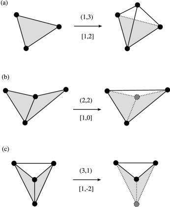
This move can be described either by dividing a triangle into three triangles by adding a vertex in the triangle, or by attaching one tetrahedron on a triangulated surface with one triangle face-to-face, which we call the $[1,2]$-moves representing changes of the volume $\Delta V$ and the surface area $\Delta S$, as shown in Fig. 2 (a).

In the similar manner the $(2,2)$-move as well as the $(3,1)$-move can be done by attaching a tetrahedron with 2 or 3 triangles glued to those neighboring triangles of the $S^{2}$-surface, which can be written in terms of $[\Delta V,\Delta S]$-moves as $[1,0]$ and $[1,-2]$ shown in Fig. 2 (b) and (c), respectively. In addition to these three moves it is also possible to make the three types of $(p,q)$-moves by detaching one tetrahedron from a $S^{2}$-surface in just the opposite manners to attaching a tetrahedron…. It is clear these six moves constitute a set of ergodic moves of triangulations for the 3-dimensional space with $D^{3}$ topology. Each move changes the number of total tetrahedron, $N_{3}$, by one unit, and at the same time it makes one of the three $(p,q)$-moves on the boundary $S^{2}$-surface. This method can be extended straightforwardly to other dimensions, such as the 2-dimensional disk, $D^{2}$, and the 4-dimensional disk, $D^{4}$ as we will see in the following sections. Each case constitutes the four and eight $[\Delta V,\Delta S]$-moves, respectively.

3 Creation of simplicial universe

When the lattice cosmological constant is below the critical value, the simplicial space tends to expand exponentially as a simulation proceeds. If we can regard this phenomenon to be the simplicial space analog of what happened in our universe at its very beginning, the inflation, the simulation can serve as a good numerical tool to study early stages of the evolution of universe. However, when we try to simulate the birth of a universe we find ourselves in a state of complete ignorance: we know neither dynamics nor initial condition. We have to recognize that there is no dynamical law to start with, since any physical law is considered to appear only at or after the space-time is settled in its classical sense. Also, there is no universe but a fluctuation at the beginning, and thus no initial condition. Under these circumstances we are forced to accept a priori elementary rules, but they should be as few as possible with the least prejudice. We shall employ an analogy of the creation of the natural number space where two rules known as the Peano axioms are essential: 1) there is an elementary unit, which is denoted by $1$, and 2) there is the next neighbor $S(a)$ of a natural number $a$. We are surprised by many profound mathematical laws such as Fermat’s last theorem hidden in this simple space.

Figure 3: 2-dimensional $[\Delta V,\Delta S]$-moves. The vertices and links on the boundary $S^{1}$ are denoted as white circles and the dash lines.

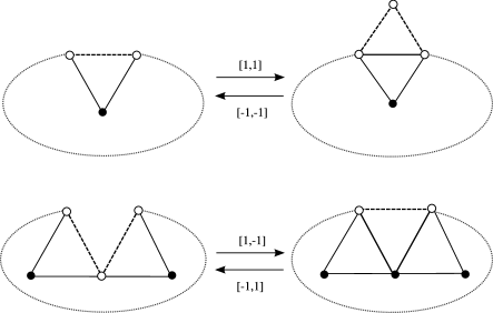
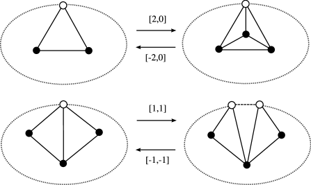
The axioms for the $d$-dimensional simplicial universe we propose are constituted by 1) there is an elementary unit of universe, which we choose a $d$-simplex, and 2) there is a set of neighbor universes $S(\alpha)$, constructed by either attaching or removing an elementary $d$-simplex to or from a universe $\alpha$. There will be many neighbor universes possible. Among them we accept only those universes which fulfill the manifold conditions: 1) at most two $d$-simplices can attach through one $(d-1)$-simplex called the face, and 2) $d$-simplices sharing one vertex form a $(d+1)$-disk, or a $(d+1)$-semi disk for the case when the vertex is on the boundary. According to our least prejudice principle this kind of manifold conditions may not be necessary, but we expect those universes which can grow indefinitely large will naturally select configurations following appropriate manifold conditions from mathematical consistency. We shall impose these manifold conditions at the beginning just for computational simplicity. However, the condition may not be unique. In Appendix B we define a different type of moves which create a manifold having more severely restricted configurations, while the manifold belongs in the same universality class. There even exist manifold conditions which allow topology changes. Inclusion of various possible topologies in the partition function is beyond the scope of this paper, and we restrict moves which conserve the topology.

Figure 4: 2-dimensional universes up to 4 triangles

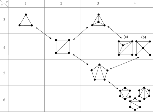
Now, let us start making a two dimensional universe as an exercise. The 2-dimensional minimum universe is a triangle, which acts also as the elementary unit. There exist four moves satisfying the manifold conditions as shown in Fig. 3, where we have denoted each move as [$\Delta N_{2},\Delta\tilde{N}_{1}$] with the boundary link number $\tilde{N}_{1}$, instead of $N_{1}$, which is related as $\tilde{N}_{1}=2N_{1}-3N_{2}$. Quantization of the simplicial universe is carried out by constructing the partition function to be a set of all the possible distinct triangulations. Possible configurations are collected as a Markov chain formed by selecting one of the four moves one after another, with appropriate weights imposed by the detailed balance condition. In Fig. 4, we show first few possible configurations up to universes made of 4-triangles. A configuration is specified by four quantum numbers, ($N_{2}$, $\tilde{N}_{1}$, $k$, $s$). The third quantum number $k$ represents the type of a diagram. For example, they are assigned to be (a) and (b) in Fig. 4 for universes with ($N_{2}=4$, $\tilde{N}_{1}=4$). The forth letter $s$ specifies the point group quantum number of a diagram with multiplicity $m_{k}$, which is $\tilde{N}_{1}$ for most of the cases except point symmetric diagrams such as Fig. 4 (b) which has $m_{k}=1$.

In general, moves are independent of the quantum number $s$, and when we denote a set of the first three quantum numbers as $a=\{N_{2},\tilde{N}_{1},k\}$, the detailed balance condition reduces to

$$\frac{p_{a}m_{a}}{n_{a}}w_{a\rightarrow b}=\frac{p_{b}m_{b}}{n_{b}}w_{b\rightarrow a},$$ (6)

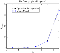
where $m_{a}$ is the point group symmetry factor of the configuration $a$. For configurations with large $N_{2}$ there are seldom diagrams having point symmetries, and we can approximate $m_{a}=\tilde{N}_{1}$, which we assume in our simulation. This assumption is checked by comparing to the matrix model prediction (Appendix A) obtained from expansion coefficients of the generating function restricting diagrams without tadpoles and self-energy insertions, for a fixed peripheral length $l$ in Fig. 6 and a fixed area $A$ in Fig. 6.

Figure 5: Number of configurations for fixed $l$ = 3.

Figure 6: Number of configurations for fixed $A$ = 20.

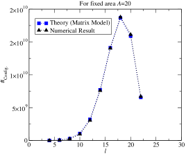
The distribution is obtained by counting the number of states with equal weight $p_{a}=1$ for each distinct configuration. The equal probability for each distinct configuration is also a natural rule for the quantized universe according to our least prejudice principle. Besides, we may give an arbitral probability $\{p_{a}\}$ through an appropriate action function $S_{a}$ as $p_{a}=\exp(-S_{a})$ depending on the purpose of a simulation. (Here, it may not be relevant to call $S_{a}$ the action for such a system without dynamics. Nevertheless, we adopt the name only because of the familiarity accustomed in statistical physics.) In $d$-dimension it is written as $\{N_{i}\}$, as

$$S^{(d)}\simeq\sum_{i=0}^{d}\mu^{(i)}N_{i}.$$ (7)

By the topological and the manifold constraints, parameters in the action function will be reduced. For the disk topology only the Euler relation is required to satisfy and the action is expressed as

$$S^{(2)}=\mu N_{2}+\mu^{B}\tilde{N}_{1},$$ (8)

in 2-dimension, where we use $\tilde{N}_{1}$ instead of the total number of links $N_{1}$. We remind these parameters are introduced only for the convenience to search possible types of universes in the followings.

Figure 7: Three types of Universes.

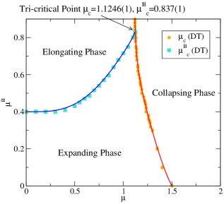
In the two dimensional parameter space ($\mu,\mu^{B}$) the numerical simulation reveals two critical lines separating into three regions corresponding to three types of universes as shown in Fig. 7. When $\mu$ is greater than the critical values $\mu_{c}$, the volume tends to decrease resulting a collapsing universe having a fate to disappear, while when $\mu$ and $\mu^{B}$ are smaller than the critical values both the volume and the surface area grow and the universe keeps expanding. The region where $\mu<\mu_{c}$ and $\mu^{B}>\mu_{c}^{B}$ the volume increases while the surface decreases and the universe looks like an elongating tube with fluctuating radii. The critical parameters $\mu_{c}=1.1247(1)$ and $\mu_{c}^{B}=0.837(1)$ at the tri-critical point coincide to the values predicted by the matrix model, which we briefly describe in the Appendix A and B for two types of manifolds.

Figure 8: The surface area distribution at the tri-critical point for a fixed volume $A=100,1000$, and $2000$.

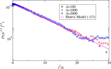
In the numerical simulation, $\mu_{c}$ can be easily identified by inspecting the tendency of volume increase. However, the critical point $\mu_{c}^{B}$ is not easily determined, because it does not cause any divergence like $\mu$. We fix this parameter so that the surface area distribution for a fixed volume coincides to the volume-area distribution function predicted by the matrix model as derived in Appendix A,

$$P_{M}(N_{2},\tilde{N}_{1})\approx N_{2}^{-2.5}\tilde{N}_{1}^{0.5}\exp\left(-\frac{1}{3}\frac{\tilde{N}_{1}^{2}}{N_{2}}\right)\exp\{-(\mu-\mu_{c})N_{2}\}\exp\{-(\mu^{B}-\mu_{c}^{B})\tilde{N}_{1}\}.$$ (9)

When we identify the volume and the peripheral length of the boundary Liouville theory and the matrix model as $A=\frac{\sqrt{3}}{4}a^{2}N_{2}$ and $l=a\tilde{N}_{1}$, the distribution function (9) is rewritten as

$$A^{-2.5}l^{0.5}\exp\left(-\frac{1}{4\sqrt{3}}\frac{l^{2}}{A}\right)\exp(-\lambda A)\exp(-\lambda^{B}l)$$ (10)

with $\lambda^{B}=(\mu^{B}-\mu_{c}^{B})/a$, which differs from the Liouville theory prediction (C $\cdot$ 10) in two points, namely the sign in front of the exponent of $l$, and the factor $2$ in the coefficient of $\frac{l^{2}}{A}$. These differences is considered to be due to the way of counting the distinct configurations. In the boundary Liouville theory those configurations which differ only in numbering of external lines are thought to be equivalent[20], and the exponent takes minus sign (Appendix C). While in the matrix model the point group symmetry factor is taken into account, and it chooses the plus sign (Appendix A,and B). The coefficient of $\frac{l^{2}}{A}$ depends on the way to choose acceptable diagrams, and in facts, the Tuute algorithm gives $192/625$ instead of $1/3$ as described in Appendix A,and B. We can perform simulations either by the matrix model convention or the Liouville theory convention selecting the multiplicity factor $m_{a}$ in Eq. (6) to be ${\tilde{N}}_{1}$ or $1$, respectively. In any way, this ambiguity will not cause any problem practically, since the multiplicity of a universe cannot be observed.

The parameter $b$ appearing in the distribution function is related to the background charge defined by $Q=b+b^{-1}$ in the Liouville theory. The exponent of $A$ is given by $-\left(\frac{Q\chi}{2b}+\frac{5}{4}\right)$ and for the disk topology the Eular characteristic $\chi=1$. For the pure gravity with the central charge $c_{L}=26$ it is known to be $b^{2}=2/3$. The numerical simulation shows the value very close to the theoretical prediction $-2.5$. The coefficient of $\frac{\tilde{N}_{1}^{2}}{N_{2}}$ in the exponent near the tri-critical point of the distribution function appears in the simulation as $0.30(4)$ as shown in Fig.[FIG_LNP] which is consistent to the theoretical value $1/3$. From these agreements between simulations and theoretical predictions in the distribution function, we feel sure that the algorithm can indeed reproduce the universe predicted by the 2-dimensional quantum gravity.

4 Introducing time and space

Without knowing what is time the definition is inevitably heuristic expecting it will appear naturally reflecting the specific property of a universe. The reason why there are two types of directions in coordinates, time and space, is a reflection of the specific topology of our universe. For a universe with the disk topology $D^{d}$ it is natural to identify the space coordinate on the boundary $S^{d-1}$, and the time coordinate along the direction perpendicular to the surface. A definition of the physical time can be found in the trivial relationship between the volume and the area of a universe,

$$V(t)=\int_{0}^{t}S(t^{\prime})dt^{\prime},$$ (11)

where $V(t)$ and $S(t)$ represent the volume ($\sim N_{d}a^{d}$) and the surface area ($\sim\tilde{N}_{d-1}a^{d-1}$), respectively. In the numerical simulation for the expanding phase both the volume and the area increase as the simulation proceeds, which we record as functions of the diffusion time $\tau$, defined by counts of the number of throwing dice in a Monte Carlo simulation. Above relation can be rewritten in terms of $\tau$ as

$$t=\int_{0}^{\tau}\frac{1}{S(\tau^{\prime})}\frac{dV(\tau^{\prime})}{d\tau^{\prime}}d\tau^{\prime},$$ (12)

indicating the growing rate of physical time is proportional to the volume increasing rate per unit area. The physical time we define has the unique direction of arrow only in the expanding universe which occurs when the cosmological constant is below the critical value. It becomes negative for the case if the volume decreases in $\tau$.

Figure 9: The ratio of $V/S$ for the expanding phase.

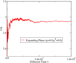
Simulations of the 2-dimensional universe in the expanding phase show the surface area increases approximately proportional to the volume as Fig. 9,

$$V(\tau)\simeq\sigma^{-1}S(\tau).$$ (13)

Thus, from the definition of the physical time, we obtain

$$t=\sigma^{-1}\log\left\{S(\tau)/S(0)\right\},$$ (14)

or $S(t)=S(0)e^{\sigma t}$, exhibiting the exponential expansion of the universe. As a matter of fact the inflational expansion is a phenomenon we expect in the classical Liouville theory with the negative cosmological constant as shown in the Appendix D. A homogeneous classical solution for the expanding mode is given by

$$e^{2b\phi(\eta)}=a^{2}(\eta)e^{2b\phi(0)},$$ (15)

where $a(\eta)=(\cos\omega\eta)^{-1}$ is the conformal scale factor at the conformal time $\eta$. The surface area of a homogeneous universe is the cross-section at $\eta$ given by $L_{\xi}/\cos(\omega\eta)$, where $L_{\xi}$ is the initial size along the conformal space coordinate $\xi$. The volume of the universe at $\eta$ is then given by

$$\int_{0}^{\eta}\frac{1}{\cos^{2}(\omega\eta^{\prime})}L_{\xi}d\eta^{\prime}.$$ (16)

We can obtain the physical time through our heuristic definition, using the volume and the surface area, which gives

$$t=\frac{1}{\omega}\log\left|\frac{1+\sin\omega\eta}{\cos\omega\eta}\right|.$$ (17)

It coincides with the standard relation between the conformal time and the physical time, $dt=a(\eta)d\eta$. Once the time coordinate is determined the space coordinate is defined on the equal time hyper-surface, $S^{d-1}$. In the 2-dimensional universe it is unique to choose the coordinate axis along the periphery.

Figure 10: Example of the 2-dimensional configuration with $(N_{2},\tilde{N}_{1})=(19,17)$.

The simplest definition of distance is the geodesic distance counting the number of links on the hyper-surface connecting two vertices with the shortest path. In terms of the distance we can measure the correlation function between points on the hyper-surface. The Liouville theory predicts the two point correlation function of the boundary primary operator $B_{\beta}(x)=\exp\{\beta\phi(x)\}$ to be

$$\left<B_{\beta}(0)B_{\beta}(x)\right>\sim\frac{1}{|x|^{2\Delta_{\beta}}},$$ (18)

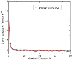
where $\Delta_{\beta}=\beta(Q-\beta)$. Assuming the coordination number of a boundary vertex corresponds to be the boundary primary operator $B_{\beta}(x)$ with $\beta=b$ in the simplicial space, we measured the correlation function of coordination numbers of two vertices on the boundary using configurations simulated with $\mu=\mu^{B}=0$. We found that this correlation function showed a delta-function type singular behavior which had not been expected at all from the Liouville theory.

Figure 11: Typical $[\Delta V,\Delta S]$-moves for the Tutte algorithm. The vertices and a link on the boundary $S^{1}$ are denoted as white circles and a dashed line.

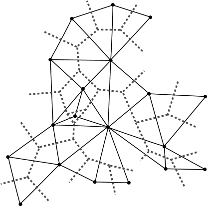
The main reason of this property was thought to come from the singular nature of the surface created under the moves we have employed. The $[\Delta V,\Delta S]$-moves were designed to generate diagrams within connected and one-particle irreducible types, forbidding tad-poles and self-energy insertions at least for the manifolds with closed topologies. However, when we applied it to generate a surface with a boundary, it was found that the one-particle irreducible nature was lost. In fact, most of the configurations had many branches on the boundary such as the one shown in Fig. 10 .

The matrix model also contains those diagrams which can be found in the table for the distribution of diagrams given in Appendix A. Under the condition of inflating space, most of the accepted moves are of the $[\Delta V,\Delta S]=[1,1]$ type, and it obviously generates an uncorrelated branches on the boundary. In order to keep diagrams within the one-particle irreducible type even for a surface with a boundary, we define a new set of moves as shown in Fig.11, consisting $[\Delta V,\Delta S]=[{\pm 2},0]$, $[1,1]$ and $[-1,-1]$. The configurations created by these moves coincide with the manifold studied by Tutte [21], which we introduce in Appendix B. The table for the distribution of diagrams generated by the Tutte algorithm clearly shows it prohibits branched surface.

Figure 12: The 2-point correlation function for the boundary operator $B^{(n)}$.

Figure 13: 2-point correlation averaged over an ensemble of $10^{4}$ universes of typically $N_{2}=10^{3}$ sizes.

Figure 14: 2-point correlation function of super-long distances, choosing one universe at $\tau=5000$, which has $N_{2}\sim 10^{3}$.

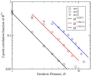
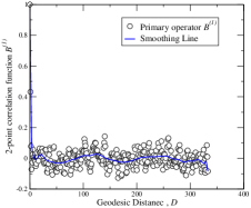
We measured the correlation function with the new configuration, but the results still exhibited the singular behavior. There seemed yet another important ingredient missing for obtaining the theoretically expected correlation function. We supposed it might be due to the improper definition of the primary operator in the simplicial space. In the previous simulations we chose the local coordination number as the simplicial primary operator. Instead, we defined a new primary operator $B^{(n)}(i)$ in the simplicial space by the average of coordination numbers of those vertices covered within $n$-steps from a vertex at $i$. Results are shown in Fig. 12 for $n=1,2,3$ using a configuration generated by the Tutte algorithm. The space dependence shows the predicted exponent, $-2$, beyond the separation $2n$ where the overlap of two operators terminates. We note that the correlation function using the old configuration remains singular even for the new operator.

In quantum gravity the range of significant correlation is typically the Planck scale reflecting the characteristic length of dynamical influence. When the space expands so rapidly, any dynamical perturbation cannot act on environments, and the quantum fluctuation will be expanded to macroscopic scale without much disturbance. In the construction of the partition function we have assumed that any possible configuration can be equally a member. As the consequence, the two point correlation function averaged over an ensemble of universes shows the short-distance nature of quantum mechanical scale shown in Fig. 14, where the long range correlation specific in each universe is wiped out after averaging over the ensemble consisting $10^{4}$ universes of $N_{2}\sim 10^{3}$ sizes.

Figure 15: Evolution of the 2-point function in the physical time $t$.

Figure 16: Power spectrum at $\tau=4000,5000\,{\rm and}\,6000$.

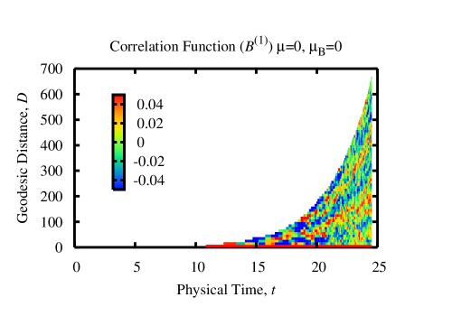
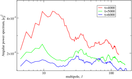
In this respect one of the most interesting phenomena of the space-time geometry can be found in the observations of CMB anisotropies. An ultimate source of the anisotropies only we can imagine is the accidental creation of a seed universe by quantum fluctuation, and random expansion of space by accumulations of elementary units according to our model. When we measure the two-point correlation function, selecting one universe as COBE and WMAP observations did, it exhibits significant super-long distance correlation as shown in Fig. 14. The pattern of this fluctuation seems to be conserved in some degree during the expansion (Fig. 15) as we have imagined in analogy to a picture on an inflating balloon. We also calculate the angular power spectrum of the two point correlation function defined by $|a_{l}|^{2}$ with

$$a_{l}=\int d\theta P_{l}(\cos\theta)f(\cos\theta),$$ (19)

where $\theta=x/r(\tau)$ is the ratio of geodesic distance and the peripheral length at $\tau$. It shows the persistence of long distance correlation Fig. 16.

5 Discussions and Conclusion

Stimulated by the recent observations on the CMB anisotropies, a model to construct a quantized universe is proposed. Reexamining the DT-method developed in the simplicial quantum gravity, we extend the algorithm so that it can create a manifold with a boundary. Numerical simulation is made mostly on the 2-dimensional universe. Three types of universes, expanding, elongating and collapsing, are observed by varying two cosmological constants. Numerical results are closely examined by comparing to the matrix model and the Liouville theory predictions, which are considered to be the consistent theories of quantum gravity in 2-dimension. The results exhibits fair agreements to the theoretical predictions. Physical time is defined based on the standard relation between volume and surface area, and the surface expands exponentially in the physical time. The exponential expansion is regarded as the quantum gravity realization of the inflation of the universe. Then, the two point correlation function on the equal-time hyper-surface is analyzed as the function of the geodesic distance. It shows the proper exponent expected by the Liouville field theory in the quantum scale after averaging over an ensemble of universes, while each universe has an extremely long distance correlation. The anisotropies originated from quantum fluctuations and the subsequent inflationary expansion is one of the most significant findings of COBE and WMAP missions.

Among many problems we need to clarify, the next step we should take is a numerical study on the universe in 4-dimension. We have already reported a few preliminary works on the algorithm and numerical results in several occasions [22]. In 4-dimension there are eight [$\Delta V,\Delta S$]-moves, corresponding to the four ($p,q$)-moves of the 3-dimensional DT and two types of attaching or removing a 4-simplex to or from the $S^{3}$ boundary for each ($p,q$)-move. Starting with a 4-simplex the Monte Carlo simulation is carried out for the partition function by constructing a Markov chain under the detailed balance condition accepting moves which fulfill the manifold conditions in exactly the same manner as the 2-dimensional simulation. The action to be used for the a priori probability $p_{a}\simeq\exp(-S_{a})$ is assumed to be

$$S=\mu N_{4}+\mu^{B}\tilde{N}_{3}+\kappa N_{2}+\kappa^{B}\tilde{N}_{1},$$ (20)

where $\kappa$ and $\kappa^{B}$ are referred to be the gravitational constant and the boundary gravitational constant. Extra two boundary terms are due to lack of relations existing in closed manifolds. Varying these parameters we can obtain several types of universes. For example, three kinds of universes similar to the 2-dimensional case are observed by varying $\mu$ and $\mu^{B}$ while two parameters, $\kappa$ and $\kappa^{B}$, are fixed to be zero. The expansion is exponential type in terms of the physical time in the simulation with $\mu=\mu^{B}=0$.

The equal-time hyper surface $S^{3}$ is considered to be a model for the very early universe. In order to appeal the fair possibility of the method we present here a comparison of the two point correlation function obtained from simulations and the WMAP data. The operator is chosen to be the scalar curvatures which are defined by the number of 4-simplices sharing one triangle. We use the simulation data of the space with the topology $D^{4}$ and $N_{4}\sim 10,000$. In its $S^{3}$ boundary we create a $B^{3}$ cavity removing about half of the total 4-simplices covered within certain geodesic distance from an arbitrarily selected 4-simplex, and regard the $S^{2}$ boundary with the area $\tilde{N}_{2}$ as the last scattering surface(lss). Then, we choose one triangle $i$ on the lss and collect all the triangles $\{j(i,x)\}$ with geodesic distance $x$ from $i$ measured in the dual lattice space. The two point correlation function is defined by

$$f(x)=\frac{1}{\tilde{N}_{2}}\sum_{i=1}^{\tilde{N}_{2}}\frac{1}{\tilde{n}_{2}(i,x)}\sum_{j(i,x)}\frac{(R_{i}-\bar{R})}{\bar{R}}\frac{(R_{j}-\bar{R})}{\bar{R}},$$ (21)

where $R_{i}$ and $\bar{R}$ are the scalar curvature at a triangle $i$ and the average over $\tilde{N}_{2}$ triangles, respectively. In order to compare to the observations, we also measure the two point correlation function of WMAP[3] in the same manner as we have done for the simulation data: choose a point $i$, collect points $\{j(i,x)\}$ with the distance $x$ apart from $i$, and calculate the temperature correlation function. The results are compared in Fig. 17.

Figure 17: Comparison of 2-point correlation functions of the 4-dimensional simulation and the WMAP third year data. Normalization constant is $f(0)$ for both cases.

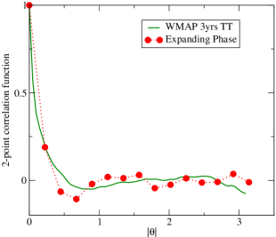
As far as the two point correlation function is concerned the agreement to the observation data is significant comparing to the $\Lambda$CDM[2].

Studies on the effects of extra two parameters to the structure of universe is one of the imminent problems. As in the 2-dimensional case, there is no reason to select specific values for these parameters. If the nature selects any, it should be the consequence of additional degrees of freedom. Therefore, the most important step we have to take is to go beyond the pure gravity by introducing the matter degrees of freedom. Without matter fields only the inflational expansion will continue forever. The universe is considered to have made a transition from the inflation to the big-bang by the deceleration effect of matter fields[23]. Following the same kind of procedures as the construction of simplicial manifold the additional variables are attached to each sub-simplex with appropriate rules for defining the neighbors. We should remember at this moment there exists no a priori laws of physics and thus no action function. The laws of physics which we expected to appear from the appropriate rules are the relativistic kinematics and quantum dynamics, which will be a primitive form of the relativistic quantum field theory.

We have just started the study of the origin of a universe in 2-dimension as the first step. It is a small universe, but the necessary step toward the universe in 4-dimension. After all there should be universes in any dimension, if it is mathematically consistent. We recall the a mathematician’s monologue[24] ‘Is mathematics reality?’. We also agree his answer the reality lies outside us, and we physicists discover dynamical laws, which is a reflection of the mathematical reality….

We would like to give our sincere thanks to Dr.’s K. Hamada, A. Zamolodchikov, and H. Kawai for their stimulating discussions and especially N. D. Hari Dass for his careful reading of the manuscript….

Appendix A Matrix model

Figure 18: Correspondence diagram between the matrix model and the triangulated manifold

The one matrix model of cubic vertex is defined by the partition function,

$$Z_{M}=\int D[M]\exp\left\{-\left(\frac{1}{2}{\rm tr}M^{2}-g{\rm tr}M^{3}\right)\right\},$$ (22)

with $N\times N$ Hermitian matrix $M$ as the dynamical variable, where

$$D[M]=\prod_{i}dM_{ii}\prod_{i>j}d[\Re M_{ij}]d[\Im M_{ij}].$$ (23)

Our main interest is one point Green’s function,

$$G_{l}(g)=\int D[M]{\rm tr}(M^{l})\exp\left\{-\left(\frac{1}{2}{\rm tr}M^{2}-g{\rm tr}M^{3}\right)\right\},$$ (24)

and its generating function $F(j,g)=\sum_{l}G_{l}(g)j^{l}$. Expanding $F(j,g)$ in powers of $g$ and $j$ as $\sum_{l,k}f_{l,k}g^{k}j^{l}$ the coefficient $f_{l,k}$ represents the number of diagrams with $k$ vertices and $l$ external lines. The significance of this coefficient lies on the fact that the dual graph of a diagram corresponds to the two dimensional triangulated manifold with $k$ triangles and $l$ boundary links as Fig. A$\cdot$1.

After a few steps of mathematical manipulations for selecting connected planer diagrams excluding tadpoles and self-energy insertions, the equation for the generating function is obtained to be[25]

$$gF^{2}-[g+j(1+s)]F+j(1+s)-gj^{2}+j^{3}=0$$ (25)

with $s(g)=gG_{3}(g)$. The first few components of Green’s function, $G_{0}(g)=1,G_{1}(g)=0$ and, $G_{2}(g)=1$, reflect the constraints which we have imposed as the acceptable diagrams. This equation contains two unknown functions, $F(j,g)$ and $s(g)$. By requiring that they are both analytic at $g=j=0$, $s(g)$ is found to satisfy

$$s^{4}+3s^{3}+8g^{2}s^{2}+3s^{2}-20g^{2}s+s+16g^{4}-g^{2}=0.$$ (26)

Expanding these equations in terms of $g$ and $j$ recursively we obtain the distribution $f_{l,k}$. We list first several coefficients in Table  1. From this table we notice that the branching polymer type diagrams such as the one with $k$ vertices and $k+2$ external lines are not forbidden. Diagrams we have accepted are the one particle irreducible type only for those without boundaries or a minimum boundary with 3-external lines. In the subsequent Appendix we introduce another type of generating function which counts only diagrams of one particle irreducible type even with a boundary.

Table 1: The coefficients $f_{l,k}$ -the distribution of diagrams with $l$-links and $k$-triangles.

$(l|k)$	1	2	3	4	5	6	7	8	9	10
3	1	0	1	0	3	0	13	0	68	0
4		2	0	5	0	20	0	100	0	570
5			5	0	21	0	105	0	595	0
6				14	0	84	0	504	0	3192
7					42	0	330	0	2130	0
8						132	0	1287	0	10296
9							429	0	5005	0
10								1430	0	19448
11									4862	0
12										16796

From the singularity analysis, $s(g)$ is shown to be singular at $g=g_{c}=\sqrt{27/256}$, and $F(j,g)$ becomes singular at $g=g_{c}$, $j=j_{c}=\sqrt{3}/4$. Logarithm of these two critical couplings correspond to the critical (lattice) cosmological constant $\mu_{c}=1.125$ and the critical (lattice) boundary cosmological constant $\mu_{c}^{B}=0.837$. Expanding at the tri-critical point the first three leading singular terms of the generating function is given by

$$F(j,g)\sim(j-j_{c})^{-\frac{3}{2}}(g-g_{c})^{\frac{3}{2}}+2^{-1}3^{-\frac{1}{2}}(j-j_{c})^{-\frac{7}{2}}(g-g_{c})^{\frac{5}{2}}+2^{-3}(j-j_{c})^{-\frac{11}{2}}(g-g_{c})^{\frac{7}{2}}+\dots.$$ (27)

Using the binomial expansion formula, $(x-x_{c})^{\alpha}=\sum_{n}Z^{\alpha}_{n}(x_{c})^{n}$, with $Z^{\alpha}_{n}\sim\frac{\sin\pi\alpha}{\pi}(-1)^{1+\alpha}n^{-(1+\alpha)}\Gamma(1+\alpha)(g_{c})^{n}$ for a large $n$, the expansion coefficient of the distribution function can be written as

$$f_{n,m}\sim m^{-2.5}n^{0.5}\exp\{-(\mu-\mu_{c})m\}\exp\{-(\mu^{B}-\mu_{c}^{B})n\}(1-\frac{1}{3}\frac{n^{2}}{m}+\frac{1}{18}\frac{n^{4}}{m^{2}}+\dots).$$ (28)

If we assume the exponential form as eq.(9) of the Liouville theory prediction the distribution function of the matrix model is expected to be

$$f_{n,m}\sim m^{-2.5}n^{+0.5}\exp\{-(\mu-\mu_{c})m\}\exp\{-(\mu^{B}-\mu_{c}^{B})n\}\exp\left(-\frac{1}{3}\frac{n^{2}}{m}\right),$$ (29)

or in terms of the area $A=\frac{\sqrt{3}}{4}a^{2}m$ and the peripheral length $l=an$, it is written as

$$P_{M}(l,A)\sim A^{-2.5}l^{0.5}\exp(-\lambda A)\exp(-\lambda^{B}l)\exp\left(-\frac{1}{4\sqrt{3}}\frac{l^{2}}{A}\right).$$ (30)

Difference of the coefficient of the $\frac{l^{2}}{A}$ from the Liouville theory by the factor $2$ is also due to the symmetric factor.

Appendix B Tutte algorithm

Tutte has been successful to obtain an equation for the generating function of the distribution of diagrams in the cubic vertex matrix model restricting within connected, and one-particle irreducible types. The generating function $T(y,x)$ are expanded as $\sum_{m,n}t_{m,n}x^{n}y^{m}$, where $n$ is the number of loops and $m+3$ is the number of external lines. The exponent $m$ and $n$ are related to the number of vertices $k$ and links $l$ of the last Appendix as $k=2n+m+1$ and $l=m+3$. The equation for $T(y,x)$ satisfies,

$$y^{2}T^{2}+(x+x{\tilde{s}}y-y-y^{2})T+y-x{\tilde{s}}=0,$$ (31)

where the unknown function ${\tilde{s}}(x)=T(0,x)$ is determined by the analyticity condition of $T(y,x)$ at $x=y=0$, which leads

$$(8x^{2}{\tilde{s}}^{2}+-20x{\tilde{s}}+32x-1)^{2}+(8x{\tilde{s}}-1)^{3}=0.$$ (32)

This equation is the same as Eq($A\cdot 4$), if we set $s=x{\tilde{s}}$ and $x=g^{2}$. The importance of the Tutte distribution function is the one-particle irreducible property of diagrams with a boundary. For example, the branching polymer type diagrams of $m+3$ external lines with zero loops are forbidden as $t_{m,0}=\delta_{m,0}$. The first few terms of the coefficients are listed in the Table 2.

Table 2: The coefficients $t_{m,n}$ -the distribution of diagrams with $(m+3)$-links and $n$-loops.

$(m|n)$	0	1	2	3	4	5	6	7	8	9
0	1	0	1	0	3	0	13	0	68	0
1		0	0	1	0	6	0	36	0	228
2			0	0	1	0	10	0	80	0
3				0	0	1	0	15	0	155
4					0	0	1	0	21	0
5						0	0	1	0	28
6							0	0	1	0
7								0	0	1
8									0	0
9										0

The singularity of ${\tilde{s}}(x)$ is identical to that of $s(x)$ of Appendix A at $x=x_{c}=27/256$, and $T(y,x)$ becomes singular at $x=x_{c}$, $y=y_{c}=3/16$, or in terms of the variables $g$ and $j$ it is at $g_{c}=\sqrt{x_{c}}$, $j_{c}=\frac{y_{c}}{\sqrt{x_{c}}}$…. Logarithm of the surface critical couplings correspond to the critical (lattice) boundary cosmological constant $\mu_{c}^{B}=0.5493$, which differs from the value given in Appendix A. The generating function is expanded near the singularity similar to the last Appendix as

$$T(y,x)\sim(j-j_{c})^{-\frac{3}{2}}(g-g_{c})^{\frac{3}{2}}+3^{\frac{3}{2}}(\frac{2}{5})^{5}(j-j_{c})^{-\frac{7}{2}}(g-g_{c})^{\frac{5}{2}}+3^{4}(\frac{2}{5})^{9}(j-j_{c})^{-\frac{11}{2}}(g-g_{c})^{\frac{7}{2}},$$ (33)

which lead the expansion coefficient of the distribution function to be

$$f_{n,m}\sim m^{-2.5}n^{+0.5}\exp\{-(\mu-\mu_{c})m\}\exp\{-(\mu^{B}-\mu_{c}^{B})n\}\exp(-\frac{192}{625}\frac{n^{2}}{m}).$$ (34)

The exponents coincide with the previous case, and the distribution function has the same asymptotic form as the previous case with the different value for $\mu_{c}^{B}$ and the coefficient in front of $\frac{n^{2}}{m}$.

We also can construct the moves which generate the diagrams satisfying the Tutte manifold conditions. They constitute four moves: $[\Delta V,\Delta S]=[2,0]$, and $[1,1]$, and their inverse moves, $[-2,0]$, and $[-1,-1]$. They are shown graphically in Fig. 3.

Appendix C Boundary Liouville field theory

The partition function of the Liouville field theory with the conformally invariant boundary is defined by[18]

$$Z_{L}=\int D[\phi]\exp\left(-A_{bulk}-A_{bound}\right).$$ (35)

The bulk Liouville action $A_{bulk}$ is given by

$$A_{bulk}=\frac{1}{4\pi}\int_{\Gamma}\left[\hat{g}^{ab}\partial_{a}\partial_{b}\phi+Q\hat{R}\phi+4\pi\lambda e^{2b\phi}\right]\sqrt{\hat{g}}d^{2}x,$$ (36)

where $\hat{R}$ is the scalar curvature associate with the background metric $\hat{g}_{ab}$ while $Q(=b+1/b)$ is the background charge. We consider only the geometry of a disk which can be represented as a simply connected domain $\Gamma$. The conformally invariant boundary action is written as

$$A_{bound}=\frac{1}{2\pi}\int_{\partial\Gamma}\left[Q\hat{K}\phi+2\pi\lambda^{B}e^{b\phi}\right]\hat{g}^{1/4}d\xi,$$ (37)

where $\hat{K}$ is the scalar curvature of the boundary associated with the background metric $\hat{g}_{ab}$. The integration over $\xi$ is taken along the boundary.

Since the partition function is invariant under a constant shift $\phi\rightarrow\phi+\frac{\sigma}{2b}$, the scaling relation,

$$Z[\lambda,\lambda^{B}]=e^{-\frac{\sigma}{2b}\chi Q}Z[\lambda e^{\sigma},\lambda^{B}e^{\sigma/2}],$$ (38)

holds, where $\chi$ is the Euler characteristic of the 2-dimensional surface. Choosing $e^{\sigma}=\lambda^{-1}$, the partition function is expected to be the homogeneous function,

$$Z[\lambda,\lambda^{B}]=\lambda^{\chi Q/2b}Z[1,\frac{\lambda^{B}}{\sqrt{\lambda}}].$$ (39)

This relation can be written in terms of the Laplace transformed variables defined by

$$Z[\lambda,\lambda^{B}]=\int_{0}^{\infty}dA\int_{0}^{\infty}dl~{}e^{-\lambda A-\lambda^{B}l}\tilde{Z}[A,l],$$ (40)

where $A$ and $l$ are the variables corresponding to the area and the boundary length of the 2-dimensional manifold, respectively. In terms of these variables the scaling relation reads,

$$\tilde{Z}[A,l]=e^{-\frac{\sigma}{2b}\chi Q-\frac{3\sigma}{2}}\tilde{Z}[e^{-\sigma}A,e^{-\sigma/2}l].$$ (41)

Choosing $e^{\sigma}=A$, we have

$$\tilde{Z}[A,l]=A^{-\left(\frac{\chi Q}{2b}+\frac{3}{2}\right)}\tilde{Z}[1,\frac{l}{\sqrt{A}}].$$ (42)

According to Ref[18] the scaling function is given by,

$$\tilde{Z}[1,\frac{l}{\sqrt{A}}]=\left(\frac{l}{\sqrt{A}}\right)^{\frac{Q}{b}-3}e^{-\frac{1}{4\sin\pi b^{2}}\frac{l^{2}}{A}}.$$ (43)

For the case of pure gravity, $b=\sqrt{2/3}$, with the disk topology, $\chi=1$, the distribution function reads,

$$\tilde{Z}[A,l]=A^{-2.5}l^{-0.5}\exp\left(-\frac{1}{2\sqrt{3}}\frac{l^{2}}{A}\right).$$ (44)

which differs from the matrix model prediction by a factor $l$. The partition function is given by

$$Z[\lambda,\lambda^{B}]=\lambda^{5/4}\left(1+\sqrt{\sin\pi b^{2}}\frac{\lambda^{B}}{\sqrt{\lambda}}\right)^{3/2}\left(1-\frac{2}{3}\sqrt{\sin\pi b^{2}}\frac{\lambda^{B}}{\sqrt{\lambda}}\right),$$ (45)

apart from a numerical factor.

There are various correlation functions known analytically. Among them we write here necessary correlation functions for the primary vertex operators, $V_{b}=e^{2b\phi}$ and $B_{b}=e^{b\phi}$,which correspond to the bulk density operator and the boundary density operator, respectively,

$$\left<V_{b}(z)\right> \simeq \frac{U(b)}{|z-\bar{z}|^{2\Delta_{b}}}$$ (46)

$$\left<B_{b}(0)B_{b}(x)\right> \simeq \frac{d(b)}{|x|^{2\Delta_{b}}},$$ (47)

where the dimension $\Delta_{\beta}=1$ for $\beta=b$. The coefficients $U(b)$ is related to the distribution function as $U(b)\sim-\frac{\partial}{\partial\lambda}Z[\lambda,\lambda^{B}]$,

$$U(b)\sim\lambda^{1/4}\left(1+\sqrt{\sin\pi b^{2}}\frac{\lambda^{B}}{\sqrt{\lambda}}\right)^{1/2},$$ (48)

while the coefficient $d(b)$ is proportional to $\frac{\partial^{2}}{\partial(\lambda^{B})^{2}}Z[\lambda,\lambda^{B}]$,

$$d(b)\sim\lambda^{1/4}\left(1+\sqrt{\sin\pi b^{2}}\frac{\lambda^{B}}{\sqrt{\lambda}}\right)^{-1/2}\left(1+2\sqrt{\sin\pi b^{2}}\frac{\lambda^{B}}{\sqrt{\lambda}}\right),$$ (49)

within a numerical factor.

Appendix D Classical Liouville equation

The Liouville field theory is considered to be valid only in the region where the stable vacuum exists. However, solutions of the classical equation of motion derived from the Liouville action,

$$S_{L}=\frac{1}{4\pi}\int d\eta d\xi\left[(\partial_{\eta}\phi)^{2}-(\partial_{\xi}\phi)^{2}+4\pi\lambda e^{2b\phi}\right],$$ (50)

are known after J. Liouville. Here, the metric is taken to be Lorenzian and the sign of the cosmological constant is opposite to the Liouville field theory. The classical equation is written as,

$$\partial_{\eta}^{2}\phi=\partial_{\xi}^{2}\phi+4\pi\lambda be^{2b\phi}$$ (51)

Changing the variables as $y=\xi+\eta$ and $z=\xi-\eta$, the solution $w(y,z)$ follows the equation

$$\partial_{y}\partial_{z}w=-\pi\lambda be^{2bw}.$$ (52)

The solution is known to have the following form,

$$e^{2bw}=-\frac{1}{\pi\lambda b^{2}}\frac{(\partial_{z}A)(\partial_{y}B)}{\{1-A(z)B(y)\}^{2}},$$ (53)

where unknown functions $A(z)$ and $B(y)$ are fixed by the initial conditions.

We consider a case when the initial conditions are given by

$$e^{2b\phi(0,\xi)}=\rho_{0}(\xi),~{}\partial_{\eta}\phi(\eta,\xi)|_{\eta=0}=0.$$ (54)

The second condition requires $B(\xi)=\pm A(\xi)$. From the positivity of the density, $e^{2b\phi(\eta,\xi)}$, we need to choose the minus sign for $\mu>0$ case. Writing $\rho(\eta,\xi)=e^{2b\phi(\eta,\xi)}$ the solution is given by

$$\rho(\eta,\xi)=\frac{\rho_{0}^{1/2}(\xi-\eta)\rho_{0}^{1/2}{(\xi+\eta)}}{{\cos^{2}\{F(\xi-\eta)-F(\xi+\eta)\}}},$$ (55)

where

$$F(\xi)=(\pi\mu b^{2})^{1/2}\int^{\xi}\rho_{0}^{1/2}(\xi^{\prime})d\xi^{\prime}.$$ (56)

For the homogeneous case, $\rho_{0}(\xi)=\rho_{0}$ (Const.), the solution is given by

$$\rho(\eta)=\frac{\rho_{0}}{\cos^{2}(\omega\eta)},~{}\omega=(4\pi\lambda b^{2}\rho_{0})^{1/2}.$$ (57)

Then the conformal scale factor $a(\eta)=e^{b\phi}$ is written as $a(\eta)=\cos^{-1}(\omega\eta)$, and the physical time $t$ defined by $dt=a(\eta)d\eta$ is expressed as

$$t=\frac{1}{\omega}\log\left|\frac{1+\sin\omega\eta}{\cos\omega\eta}\right|,$$ (58)

or $\cosh\omega t=1/\cos(\omega\eta)$. The boundary length $a(\eta)l_{0}$ represented in terms of the physical time is expanding exponentially as $l(t)=l(0)\cosh(\omega t)$.