Non-Perturbative Decay of a Monopole:
the Semiclassical Pre-Exponential Factor

Abstract

The rate of the non-perturbative decay of a ’t Hooft–Polyakov monopole in an external electric field into a dyon and a charged fermion is calculated. The sub-leading semiclassical pre-exponential factor is presented for the first time for this process. The leading exponential factor is shown to be in full agreement with the previous results derived in a different technique. Analogous treatment is shown to hold for the two-fermionic decay of the lightest bound state in Thirring model. Thus restoring the “effective meson–fermion vertex” becomes possible.

I Introduction

The physics of magnetic monopoles has attracted attention for a long time. Charge quantization Dirac:1948um , baryon decay Rubakov:1984bw , duality in gauge theories Montonen:1977sn , confinement description Seiberg:1994rs are just a few examples of important issues associated with monopoles.

The ’t Hooft–Polyakov monopole, which will be the main object of our study, is stable; its decay is impossible unless some external field comes into play. There exists a growing interest to the spontaneous and induced Schwinger decay processes in external fields, as well as to the induced vacuum decay processes, see e.g. Gorsky:2001up . Therefore it is natural to study the non-perturbatively allowed decay of a monopole into a dyon and a fermion. This paper is organized as follows. In Section II some general facts on monopole physics and induced decays are reviewed. We examine the conditions under which a semiclassical treatment is valid for the considered problem. The decay rate is calculated in Section III. The elaborated technique is simplified and applied to the bound state decay of the Thirring model in Section IV, and the results are summarized in Section V.

II Preliminaries

II.1 Monopoles: Non-Perturbative and Non-Local Objects

Since the historic paper by Dirac Dirac:1948um the question how to incorporate the dynamics of magnetic monopoles into the standard quantum field-theoretical paradigm has been non-trivial. Treating monopoles and charges within the same framework is hindered by the two obstructions: inapplicability of the perturbation theory and non-locality.

Due to Dirac’s quantization condition Dirac:1931kp , the charge $g$ of a monopole is $g^{2}\sim\frac{1}{\alpha}\sim 137$ so that no reasonable perturbation series can be derived with respect to this parameter, unlike the standard QED perturbation theory in powers of $\alpha$. Several attempts have been made to elaborate a self-contained QED with monopoles Zwanziger:1970hk ; Gamberg:1999hq .

These two fundamental problems inevitable for the point-like Dirac monopoles arise under a different guise for the ’t Hooft–Polyakov monopole. The monopole configuration is a priori a solution to the classical field equations. It exhibits some properties of a point particle, but it cannot be treated as if it were generated by some local field operator. The ’t Hooft–Polyakov monopole should be thought of as a kind of semiclassical object rather than a quantum particle since its characteristic size is roughly $1/\alpha$ times greater than its de Broglie wavelength. In the dual theory Montonen:1977sn the monopoles correspond to the original gauge bosons, which do have a local description; however, in the original theory itself no local description is possible.

The non-perturbative issues of monopole dynamics can be studied via geometric and topological methods, permitting description of dynamics of monopoles and dyons in terms of geodesics on the moduli spaces of solutions to the Bogomolny equations Atiyah:1985fd ; Gibbons:1986df . Processes which have an explicit quantum field-theoretical interpretation like scattering of monopoles into monopoles or dyons have been shown to take place. However, no quantum field theoretical model of these processes exists so far.

String theory suggests describing dyons as $(p,q)$ strings with ends fixed on some D-branes Polchinski:1998rq . This description was recently proposed to induce the process “gauge boson $\to$ monopole, dyon” or “monopole $\to$ dyon, charge” in an external field  by Gorsky, Saraikin and Selivanov Gorsky:2001up . The existence of a corresponding vertex in string theory is mentioned to show that there are some attempts to elaborate a local perturbative-like treatment of monopoles. The string vertex is not directly used in the calculations below. However, its existence provides us with a heuristic apology to validate introducing an “effective coupling”, which is absent at the perturbation theory level.

There exists a wide class of processes in field theory becoming non-perturbatively allowed once an external field comes into play. The obvious example is the Schwinger spontaneous $e^{+}e^{-}$ pair production in an external electric field (for a review see Dunne:2004nc ), or an analogous process for the spontaneous Schwinger-like monopole pair production in the static magnetic field Affleck:1981ag . Another class of non-perturbative phenomena consists of false vacuum decay processes in a scalar field theory. The generic case of false vacuum decay in a distorted Higgs-like potential was initially discussed in Kobzarev:1974cp ; Coleman:1977py . There exists a deep similarity between spontaneous Schwinger processes and false vacuum decay. Formally, these two phenomena are identical in $1+1$ dimensions Voloshin:1985id . The action $S_{cl}$ of a classical configuration of $e^{+}e^{-}$ paths in Euclidean domain contributing to the semiclassical pair creation probability $w\sim e^{-S_{cl}}$ behaves like “$const_{1}\mathrm{(volume)}-const_{2}\mathrm{(surface)}$”. The same behaviour is typical for the action of a classical bubble in the thin wall approximation, describing, in its turn, a semiclassical vacuum decay probability. This statement can be considered as a hint to a better understanding of more general cases for the both types of processes.

II.2 Induced vs. Spontaneous

History of the false vacuum decay teaches us a lesson that if a process is possible as a spontaneous one, there should exist related induced ones Affleck:1979px ; Selivanov:1985vt . The same argument works for the Schwinger processes. A possibility of an induced Schwinger-type monopole decay was first suggested in Gorsky:2001up . Monopoles were first treated as triggers for vacuum decay in a scalar field theory long ago Steinhardt:1981ec .

This interpretation allows one to symbolically introduce an effective “charge–monopole–dyon” vertex, although it does not exist at the level of perturbation theory. As in our previous papers Monin:2005wz ; Monin:2006dt , ’t Hooft–Polyakov monopole is treated as a semi-classical object, for which the notion of the trajectory is well defined. Only trajectories far larger than the monopole size are dealt with, in order not to break down the semiclassical approximation. The trajectory of the monopole is analytically continued into the Euclidean domain, where a correction to its Green function is calculated, yielding the decay rate.

We can not describe monopole in terms of a second-quantized theory. What is meant here then by “the Green function of a monopole”? This Green function stands for an effective one-particle description. One is incapable of writing down a quantum field theoretical path integral for it, nevertheless, a 1-particle quantum-mechanical path integral for a particle with a given spin, electric charge $e$ and magnetic charge $g$ in an external vector-potential $A_{\mu}$ is meaningful in the semiclassical approximation.

The close relation of the present problem to the issue of false vacuum induced decay has already been pointed out. In the course of calculations, both problems are dealt in a semiclassical technique very close to that of world-line instantons by Dunne and Schubert Dunne:2005sx . Therefore, the structure of the result is similar:

$$\Gamma\sim Ke^{-S_{cl}},$$

where the leading exponent behavior is governed by the action on a classical configuration $S_{cl}$, be it a field distribution in field theory or a 1-particle trajectory in quantum mechanics; the subleading pre-exponential factor $K$ generally costs more efforts to be extracted Dunne:2006st . It contains the fluctuation determinants as well as contributions from Jacobians, which arise when integrating out the collective coordinates.

Basically, two techniques exist for calculating this prefactor. One can either study the fluctuation determinant of the operator describing oscillations around the classical solutions Kiselev:1975eq or one can reduce the field-theoretical problem to that of 1-particle relativistic quantum mechanics and obtain the prefactor in terms of the WKB method Voloshin:1985id .

The level of complexity of the prefactor calculation depends on the method applied. E.g., the prefactor in Schwinger’s derivation of $e^{+}e^{-}$ production rate comes at the same price with the exponent. On the other hand, when time-dependent field enters the play it often comes out to be useful to calculate the determinants via the Gelfand–Yaglom or Levit–Smilansky Levit:1976fv method, or via the Riccati equation method Kleinert:2004ev .

In a paper by one of us (A.K.M.) Monin:2005wz the monopole decay was studied by means of Feynman path integrals in the leading semiclassical approximation. Proof of the existence of a negative mode in the spectrum was also given, however, the full fluctuation determinant was not calculated. In our preceding paper this technique was extended to inhomogeneous fields Monin:2006dt . Here a calculation giving the exponential and the pre-exponential factor simultaneously is presented.

III Monopole in 4D

A monopole with a magnetic charge $g$, mass $M_{m}\sim M_{W}/\alpha$ ($M_{W}$ is the $W$-boson mass) is considered in a constant external electric field in a four-dimensional space-time. The rate of its decay into a dyon of mass $M_{d}$ with electric and magnetic charges $e,g$ respectively, and a charged fermion of mass $m_{e}$ will be calculated. First the reader is reminded how Green functions can be obtained for an electrically and magnetically charged particle in an external field. Then a “loop correction” is calculated, although this notion has a limited applicability, as commented above.

It has already been mentioned that the monopole Green function has got only a semiclassical meaning in the proposed approach. This means that one is bound by the requirement for the charge-dyon loop to be larger than the ’t Hooft–Polyakov monopole size. Technically this will imply taking all loop integrals in the saddle-point approximation. On the other hand, the saddle–point approximation does a good job: it yields the imaginary part of mass correction directly, avoiding the infinite real mass renormalization part .

A self-consistent field-theoretical treatment of Abelian monopoles not requiring introduction of Dirac strings was performed by Zwanziger. Let us consider fermionic fields $\psi_{i}$ carrying both electric charge $e_{i}$ and magnetic charges $g_{i}$. Then two $U(1)$ currents will be describing the interaction of the system with the external field, electric current $j_{e}$ and magnetic current $j_{g}$

$$j_{e}^{\mu}=\sum_{i}e_{i}\bar{\psi}_{i}\gamma^{\mu}\psi_{i}$$ (1)

$$j_{g}^{\mu}=\sum_{i}g_{i}\bar{\psi}_{i}\gamma^{\mu}\psi_{i}$$ (2)

which are subject to condition

$$\begin{array}[]{l}F^{\mu\nu}=\partial^{\mu}A^{\nu}-\partial^{\nu}A^{\mu}+(\mbox{non-local terms})\\ \tilde{F}^{\mu\nu}=\partial^{\mu}\tilde{A}^{\nu}-\partial^{\nu}\tilde{A}^{\mu}+(\mbox{non-local terms})\end{array}$$ (3)

Interaction Lagrangian will then be organized as

$$L_{int}=j_{\mu}^{e}A^{\mu}+j_{\mu}^{g}\tilde{A}^{\mu}$$ (4)

It is argued by Zwanziger Zwanziger:1970hk that the non-local terms have zero-measure support and thus they can be neglected for practical purposes. Moreover, in present case the non-local terms may be neglected due to the non-Abelian nature of the initial field configuration.

The Green function for a scalar particle with electric charge $e$ and magnetic charge $g$ can be given in terms of first-quantized formalism suggested by Affleck et al. Affleck:1981bm

$$G(y,x)=\int dse^{im^{2}s}\int^{\tiny\hbox to0.0pt{$\displaystyle x(s)=y$\hss}}_{\tiny\hbox to0.0pt{$\displaystyle x(0)=x$\hss}}\mathcal{D}x(t)e^{i\int_{0}^{s}\dot{x}^{2}/4+e\int A_{\mu}dx^{\mu}+g\int\tilde{A}_{\mu}dx^{\mu}}$$

In a constant external field this can be calculated exactly. On the other hand, this Green function is nothing else than the matrix element

$$G(y,x)=\left\langle y\left|\frac{1}{D^{2}+m^{2}}\right|x\right\rangle.$$

The covariant derivative for a particle with both electric and magnetic charges $e$ and $g$ in an external field should look like

$$D_{\mu}=\partial_{\mu}+ieA_{\mu}+ig\tilde{A}_{\mu}.$$

This was justified by Gibbons and Manton Gibbons:1995yw .

First-quantized treatment exists for fermions as well, but it is easier for us to write down the fermionic Green function by virtue of similarity

$$G_{F}(y,x)=\left\langle y\left|\frac{1}{m-i\hat{D}}\right|x\right\rangle$$

Consider now a constant electric field ${\bf E}=(0,0,E)$. Let us choose a vector potential in the form $A_{\mu}(x)=\frac{E}{2}(-x_{3},0,0,x_{0})$, hence $\tilde{A}_{\mu}=\frac{E}{2}(0,-x_{2},x_{1},0)$. The Dirac operator takes the form

$$i\hat{D}-m=i\gamma^{\mu}D_{\mu}-m=i\gamma^{\mu}(\partial_{\mu}+ieA_{\mu}+ig\tilde{A}_{\mu})-m.$$ (5)

A propagator of a fermionic particle with an electric charge $e$ and magnetic charge $g$ is given by

$$G_{F}(y,x)=(m+i\hat{D_{y}})G^{(0)}(y,x),$$ (6)

where the following auxiliary function is introduced

$$\begin{array}[]{lll}\displaystyle G^{(0)}(y,x)&=&-\displaystyle\frac{i}{32\pi^{2}}\,egE^{2}\times\\ &\times\displaystyle\int\limits_{0}^{\infty}&\!\displaystyle ds\frac{\mathrm{e}^{i\frac{(m^{2}+i\epsilon)s}{2}}\mathrm{e}^{-\frac{1}{2}(eEs\gamma^{0}\gamma^{3}+gEs\gamma^{1}\gamma^{2})}\mathrm{e}^{iS}}{\sinh\left(\frac{eEs}{2}\right)\sin\left(\frac{gEs}{2}\right)}\end{array}$$ (7)

Terms $i\epsilon$ will be omitted further. Here

$$\begin{array}[]{lll}S=\frac{eE}{4}(y-x)_{\|}^{2}\coth\frac{eEs}{2}+\frac{eE}{2}(y_{0}x_{3}-y_{3}x_{0})+\\ +\frac{gE}{4}(y-x)_{\bot}^{2}\cot\frac{gEs}{2}+\frac{gE}{2}(y_{1}x_{2}-y_{2}x_{1}),\end{array}$$ (8)

indices $\|$ and $\bot$ denote the $(0,3)$ and $(1,2)$ components of 4-vector correspondingly. Deforming the $s$ integration contour (roughly speaking, turning it like $s\to is$) and making a transition to Euclidean quantities like $x_{0}\to-ix_{0}$, one writes down the Euclidean Green function

$$\begin{array}[]{lll}G_{E}^{(0)}(y,x)&=&\displaystyle\frac{1}{32\pi^{2}}\,egE^{2}\times\\ &\times\displaystyle\int\limits_{0}^{\infty}&\!\displaystyle ds\frac{\mathrm{e}^{-\frac{m^{2}s}{2}}\mathrm{e}^{\frac{1}{2}(eEs\gamma^{0}\gamma^{3}+igEs\gamma^{1}\gamma^{2})}\mathrm{e}^{-S_{s}}}{\sin(\frac{eEs}{2})\sinh(\frac{gEs}{2})}\,,\end{array}$$ (9)

where

$$\begin{array}[]{l}S_{s}=\frac{eE}{4}(y-x)_{\|}^{2}\cot\frac{eEs}{2}-\frac{eE}{2}(y_{0}x_{3}-y_{3}x_{0})+\\ +\frac{gE}{4}(y-x)_{\bot}^{2}\coth\frac{gEs}{2}-i\frac{gE}{2}(y_{1}x_{2}-y_{2}x_{1}),\end{array}$$

all the four-vectors in this expression are supposed to be taken in Euclidean space with the positive overall metric sign; the index $E$ will be omitted further. The fermionic propagator thus takes the form

$$G_{F}(y,x)=\left(m+\gamma^{\mu}a_{\mu}(y,x)\right)G^{(0)}(y,x),$$ (10)

where

$$\begin{array}[]{lll}a_{\|}(y,x)&=&\Bigl{(}\frac{eE}{2}(y_{0}-x_{0})\cot\alpha+\frac{eE}{2}(y_{3}-x_{3}),\\ &&\qquad\frac{eE}{2}(y_{3}-x_{3})\cot\alpha-\frac{eE}{2}(y_{0}-x_{0})\Bigr{)},\\ a_{\bot}(y,x)&=&\Bigl{(}\frac{gE}{2}(y_{1}-x_{1})\coth\beta+i\frac{gE}{2}(y_{2}-x_{2}),\\ &&\qquad\frac{gE}{2}(y_{2}-x_{2})\coth\beta-i\frac{gE}{2}(y_{1}-x_{1})\Bigr{)},\end{array}$$ (11)

with $\alpha=\frac{eEs}{2}$ and $\beta=\frac{gEs}{2}$.

There are arguments in favour of thinking (0,1)-monopole to be a scalar particle and a (1,1)-dyon to be a spin-$\frac{1}{2}$ particle Coleman:1982cx , thus fermionic Green function above refers to dyons. It describes charged fermions as well in the limit $g=0$.

The correction to monopole’s Green function propagating from $(0,0,0,0)$ to $T=(0,0,0,T)$ may be expressed in terms of Feynman path integrals Monin:2005wz and reduced to a contraction of Green functions (here the “effective vertex” of monopole-dyon-charged fermion interaction is suggested to be of the form $\,\lambda\phi\bar{\psi}\psi$)

$$\begin{array}[]{lll}\delta G_{m}(T,0)&=&\displaystyle\lambda^{2}\int G_{m}(z,0)G_{m}(T,w)\times\\ &&\qquad\displaystyle\times\>\mathrm{tr}[G_{e}(w,z)G_{d}(w,z)]dw\,dz,\end{array}$$ (12)

$\lambda$ being (an unknown) dimensionless factor, indices $m,e,d$ belonging here and everywhere below to a monopole, a charged fermion, and a dyon respectively. Substituting the above Green functions for their Schwinger representations (7), one can express the trace in (12) in terms of Schwinger parameters $\alpha_{i}$

$$\begin{array}[]{lll}\mathrm{Tr}&\equiv&\mathrm{tr}(M_{d}+\hat{a})(\cos\alpha_{2}+\gamma^{0}\gamma^{3}\sin\alpha_{2})\times\\ &\times&(\cosh\beta_{2}+i\gamma^{1}\gamma^{2}\sinh\beta_{2})\times\\ &\times&(m_{e}+\hat{b})(\cos\alpha_{1}-\gamma^{0}\gamma^{3}\sin\alpha_{1}),\end{array}$$ (13)

here $a$, $\alpha_{2}$, $\beta_{2}\equiv\frac{g}{e}\alpha_{2}$ correspond to the dyon propagator and $b$, $\alpha_{1}$ to that of the charged fermion. Schwinger parameters $\alpha_{3}$, $\alpha_{4}$ coresponding to monopole propagation are also present in (12). Calculating the trace one obtains

$$\begin{array}[]{lll}\mathrm{Tr}&=&\displaystyle 4\Biggl{(}(m_{e}M_{d}\cosh(\frac{g}{e}\alpha_{2})\cos(\alpha_{1}-\alpha_{2})+\\ &+&\displaystyle\left(\frac{eE}{2}\right)^{2}(w-z)_{\|}^{2}\frac{\cosh(\frac{g}{e})\alpha_{2}}{\sin\alpha_{1}\,\sin\alpha_{2}}+\\ &+&\displaystyle\frac{egE^{2}}{4}(w-z)_{\bot}^{2}\frac{\cos(\alpha_{1}-\alpha_{2})}{\sinh(\frac{g}{e}\alpha_{2})}\Biggr{)}.\end{array}$$

Performing Gaussian integrals over $z$ and $w$, and introducing Feynman variables $\alpha_{3}=Ax,\alpha_{4}=A(1-x),$ with the Jacobian of the substitution being $A$, one notes that no dependence on $x$ enters formula (12), thus the $x$-integration is taken off trivially, after which the correction to Green function becomes

$$\begin{array}[]{lll}\delta G&=&const\displaystyle\int\frac{d\alpha_{1}\,d\alpha_{2}\,A\,dA}{\alpha_{1}\,\sin\alpha_{1}\,\sin\alpha_{2}\,\sinh(\frac{g}{e}\alpha_{2})}\displaystyle\frac{\displaystyle\mathrm{\displaystyle e}^{-\left[\frac{m_{e}^{2}}{eE}\alpha_{1}+\frac{M_{d}^{2}}{eE}\alpha_{2}+\frac{M_{m}^{2}}{eE}A+\frac{\frac{eE}{4}T^{2}}{A+\frac{\sin\alpha_{1}\,\sin\alpha_{2}}{\sin(\alpha_{1}+\alpha_{2})}}\right]}}{\displaystyle\Bigl{[}\bigl{(}\frac{e}{\alpha_{1}}+g\cot\frac{g\alpha_{2}}{e}\bigr{)}\sinh\frac{gA}{e}+g\cosh\frac{gA}{e}\Bigr{]}\displaystyle\bigl{[}A(\cot\alpha_{1}+\cot\alpha_{2})+1\bigr{]}}\times\\ &\times&\displaystyle\Biggl{\{}m_{e}M_{d}\cosh(\frac{g}{e}\alpha_{2})\cos(\alpha_{1}-\alpha_{2})+\displaystyle eE\frac{\cosh(\frac{g}{e}\alpha_{2})A}{\sin\alpha_{1}\,\sin\alpha_{2}[A(\cot\alpha_{1}+\cot\alpha_{2})+1]}+\\ &+&\displaystyle\Bigl{(}\frac{eET}{2}\Bigr{)}^{2}\frac{\cosh(\frac{g}{e}\alpha_{2})}{\sin\alpha_{1}\,\sin\alpha_{2}[A(\cot\alpha_{1}+\cot\alpha_{2})+1]^{2}}+\displaystyle\frac{egE\cos(\alpha_{1}-\alpha_{2})\,\sinh(\frac{g}{e}A)}{\alpha_{1}\sinh(\frac{g}{e}\alpha_{2})\displaystyle\Bigl{[}\bigl{(}\frac{e}{\alpha_{1}}+g\cot\frac{g\alpha_{2}}{e}\bigr{)}\sinh\frac{gA}{e}+g\cosh\frac{gA}{e}\bigr{)}\Bigr{]}}\Biggr{\}}.\end{array}$$ (14)

To integrate over variable $A$, the saddle-point approximation is employed. Generally, the saddle-point approximation works for the integrals

$$\int_{0}^{+\infty}e^{\nu f(s)}g(s)ds=\sqrt{\frac{2\pi}{-\nu f^{\prime\prime}(s_{0})}}e^{\nu f(s_{0})}g(s_{0})+\mathrm{O}\left(\frac{1}{\nu}\right)$$ (15)

[$s_{0}$ being the minimum point of $f(s)$], when $\nu\to\infty$. In the present case,

$$\nu f(A)=-\frac{M_{m}^{2}}{eE}\left[A+\frac{(eE)^{2}}{4M_{m}^{2}}T^{2}\frac{1}{A+const}\right]$$ (16)

satisfies this requirement since $\nu=\frac{M_{m}^{2}}{eE}$ is a large parameter indeed, coefficient $\frac{(eE)^{2}}{4M_{m}^{2}}T^{2}$ being not infinitesimal as $T$ may be made large enough for our purposes. In fact, the limit $T\to\infty$ will be used, so the latter statement is fairly justified.

The saddle point value $A_{0}$ in the integral (14) over $A$ is assumed to satisfy $A_{0}\gg 1$, so in principle one could consider asymptotics for hyperbolic functions in the form $\sinh\frac{gA}{e}\approx\cosh\frac{gA}{e}\approx\frac{1}{2}\,\mathrm{e}^{\frac{gA}{e}}$, and raise $\frac{gA}{e}$ to the exponent. However, one should remember that since the monopole and the dyon are being treated as point-like particles, it is obligatory to consider an external field small enough so that the size of the loop (see Fig. 1) is larger than the size of the monopole.

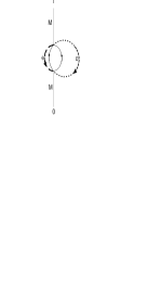
Figure 1: Classical paths in $(x_{3},x_{0})$ plane with arbitrary winding numbers.

For such a field it is easy to show that $\frac{M^{2}_{m}}{gE}\gg g^{2}$. So the term $gA/e$ must be neglected in the exponent compared to $m^{2}A/eE$. But $gA/e$ is still large enough to consider hyperbolic functions $\cosh(\frac{g}{e}A)$ and $\sinh(\frac{g}{e}A)$ approximately equal. Then the saddle point value for $A$ is

$$A_{0}=\frac{eET}{2M_{m}}-\frac{\sin\alpha_{1}\/\sin\alpha_{2}}{\sin(\alpha_{1}+\alpha_{2})},$$

and the second derivative is

$$\frac{\partial^{2}f}{\partial A^{2}}=\frac{4M_{m}^{3}}{(eE)^{2}T}.$$

In order to find the monopole mass correction one should know the asymptotic form of the propagator of a scalar particle in an external field. The scalar Euclidean propagator has the following asymptotics

$$G_{m}(T,0)=\frac{1}{16\pi^{3/2}}\frac{gE}{\sqrt{M_{m}T}}\,\frac{\mathrm{e}^{-M_{m}T}}{\sinh\frac{gET}{2M_{m}}},$$ (17)

and the leading-order (in powers of $T$) contribution to its variation due to the variation of the monopole mass

$$\delta G_{m}(T,0)=-\frac{1}{8\sqrt{2}\pi^{3/2}}\delta M_{m}\,gE\sqrt{\frac{T}{M_{m}}}\,\frac{\mathrm{e}^{-M_{m}T}}{\sinh\frac{gET}{2M_{m}}}.$$ (18)

Comparing this result with the one obtained after integration (14) over $A$ one gets the mass correction

$$\begin{array}[]{lll}\delta M_{m}&=&\displaystyle\frac{\lambda^{2}g}{(32\pi)^{3/2}M}\displaystyle\int\frac{d\alpha_{1}\,d\alpha_{2}}{\alpha_{1}\,\sinh(\frac{g}{e}\alpha_{2})\,\sin(\alpha_{1}+\alpha_{2})}\times\vspace{0.4cm}\\ &\times&\frac{\displaystyle\mathrm{\displaystyle e}^{\displaystyle-\left(\frac{m_{e}^{2}}{eE}\alpha_{1}+\frac{M_{d}^{2}}{eE}\alpha_{2}-\frac{M_{m}^{2}}{eE}\frac{\sin\alpha_{1}\,\sin\alpha_{2}}{\sin(\alpha_{1}+\alpha_{2})}\right)}\vspace{0.2cm}}{\displaystyle\bigl{(}\frac{e}{\alpha_{1}}+g\cot(\frac{g}{e}\alpha_{2})+g\bigr{)}}\times\\ &\times&\displaystyle\biggl{[}m_{e}M_{d}\cosh\left(\frac{g\alpha_{2}}{e}\right)\cos(\alpha_{1}-\alpha_{2})+\\ &&\displaystyle\qquad+M_{m}^{2}\cosh\left(\frac{g\alpha_{2}}{e}\right)\frac{\sin\alpha_{1}\sin\alpha_{2}}{\sin^{2}(\alpha_{1}+\alpha_{2})}\biggr{]}.\end{array}$$ (19)

The terms proportional to $E$ compared to the ones proportional to any bilinear combination of masses have already been neglected here. It was reasonable to leave them out since such an assumption had already been taken when integrating over $A$ in the saddle-point technique. The last step is to integrate over $\alpha_{1}$ and $\alpha_{2}$ using the saddle point method. Note that the custom integration via methods of the theory of complex variable functions fails, due to an essential non-analyticity in $\alpha_{1}+\alpha_{2}$ present in the expression being studied (roughly speaking, it is like $e^{-1/z}$ in the vicinity of $z=0$, as can be seen from (19) above). On the contrary, saddle-point approximation remains valid, because all massive parameters are considered to be large compared to $\sqrt{eE}$.

However, due to the specified essential singularities, a complicated deformation of the integration contour should be performed. Formula (19) should rather be understood in the following way: one starts with the Minkowskian Green functions, for which path of integration is directed along the imaginary axis of $z\equiv\alpha_{1}+\alpha_{2}$, being away from essential singularities. Such a contour rotation refers not only to (19), but to (6) and (7) as well. The original Minkowskian Green function was defined with a contour directed along imaginary $s$ axis. When writing down the Euclidean Green function (6), one should already have given a prescription for turning the integration contour to the real $s$ axis. How it should have been done is shown in Fig. 2.

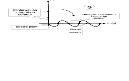
Figure 2: Integration contour for Minkowskian and Euclidean Green Functions.

Here singularities do not lie on integration path; and saddle-points are passed in the (imaginary) direction prescribed by steepest descent condition. The deformation was performed in the domain of analyticity of the integrand, without traversing the singularities. The integral is dominated by saddle points, and may be evaluated as sum of integrals in the vicinities of each saddle-point. A contour (of real dimension 2) in $\mathbb{C}^{2}$ for (19) is constructed in a similar way. It is not shown here due to high dimensionality.

The function $f(\alpha_{1}\,,\alpha_{2})=\frac{m_{e}^{2}}{eE}\alpha_{1}+\frac{M_{d}^{2}}{eE}\alpha_{2}-\frac{M_{m}^{2}}{eE}\frac{\sin\alpha_{1}\,\sin\alpha_{2}}{\sin(\alpha_{1}+\alpha_{2})}$ is to be minimized. One gets the saddle point values $\theta_{i}^{(n)}$ for $\alpha_{i}$, which come out to be the same as were obtained in Monin:2005wz by a different method

$$\begin{array}[]{lllllll}\left(\begin{array}[]{c}\theta_{1}^{\pm(n)}\\ \theta_{2}^{\pm(m)}\end{array}\right)&=&\pm\left(\begin{array}[]{c}\cos^{-1}\frac{M_{m}^{2}+m_{e}^{2}-M_{d}^{2}}{2m_{e}M_{m}}\\ \cos^{-1}\frac{M_{m}^{2}-m_{e}^{2}+M_{d}^{2}}{2M_{d}M_{m}}\end{array}\right)+\left(\begin{array}[]{c}2\pi n\\ 2\pi m\end{array}\right)\equiv\\ &\equiv&\left(\begin{array}[]{c}\pm\theta_{1}+2\pi n\\ \pm\theta_{2}+2\pi m\end{array}\right),\\ &&n,\,m\in\mathbb{Z},\theta_{i}^{\pm(n)}>0\par\end{array}$$

the corresponding determinant being

$$\begin{array}[]{lll}\displaystyle\det\vphantom{|}_{ij}\left(\frac{\partial^{2}f}{\partial\alpha_{i}\partial\alpha_{j}}\right)&=&\displaystyle-4\frac{\sin^{2}\theta_{1}\,\sin^{2}\theta_{2}}{\sin^{4}(\theta_{1}+\theta_{2})}\left(\frac{M_{m}^{2}}{eE}\right)^{2}=\\ &=&\displaystyle-4\frac{(m_{e}M_{d})^{2}}{(eE)^{2}}.\end{array}$$ (20)

One can see that there exists a two-parameter family of local minima of the saddle-point integral. Geometrically, the integer parameters $m,n$ denote multiply-wound classical solutions. The result is a sum over all saddle points. The physical meaning of such a sum was discussed in Monin:2006dt . The semiclassical approximation counts all possible classical sub-barrier trajectories, which are arcs of a circle, $\theta_{i}$ having direct meaning of an angular coordinate on the particle trajectory in the Euclidean plane, taking them with weights $e^{-S^{\pm}_{n,m}}$ given below.

Finally one obtains the mass correction as a sum over winding numbers $m,n$

$$\begin{array}[]{lll}\displaystyle\mathrm{Im}\,\delta M_{m}&=&\displaystyle-\frac{\lambda^{2}}{8\pi}\,\displaystyle\frac{eE}{M_{m}}\displaystyle\left\{\displaystyle\sum_{n,m=0}\frac{\mathrm{e}^{-S^{+}_{n,m}}\cos^{2}(\frac{\theta_{1}-\theta_{2}}{2})}{\sin(\theta_{1}+\theta_{2})\bigl{(}\frac{e}{\theta_{1}+2\pi n}+g\cot(\frac{g}{e}(\theta_{2}+2\pi m))+g\bigr{)}}\right.\displaystyle\frac{g}{(\theta_{1}+2\pi n)\tanh(\frac{g}{e}(\theta_{2}+2\pi m))}\,-\\ &-&\left.\displaystyle\sum_{n,m=1}\frac{\mathrm{e}^{-S^{-}_{n,m}}\cos^{2}(\frac{\theta_{1}-\theta_{2}}{2})}{\sin(\theta_{1}+\theta_{2})\bigl{(}\frac{e}{2\pi n-\theta_{1}}+g\cot(\frac{g}{e}(2\pi m-\theta_{2}))+g\bigr{)}}\displaystyle\frac{g}{(2\pi n-\theta_{1})\tanh(\frac{g}{e}(2\pi m-\theta_{2}))}\right\},\end{array}$$

with

$$\begin{array}[]{lll}S_{n,m}^{+}&=&\frac{m_{e}^{2}}{eE}\,\theta_{1}^{+(n)}+\frac{M_{d}^{2}}{eE}\,\theta_{2}^{+(m)}-\frac{m_{e}M_{d}}{eE}\sin(\theta_{1}+\theta_{2}),\vspace{0.2cm}\\ S_{n,m}^{-}&=&\frac{m_{e}^{2}}{eE}\,\theta_{1}^{-(n)}+\frac{M_{d}^{2}}{eE}\,\theta_{2}^{-(m)}+\frac{m_{e}M_{d}}{eE}\sin(\theta_{1}+\theta_{2}).\end{array}$$

This sum looks rather ugly, however, the contributions of higher winding paths are suppressed by the factor of $\exp[-(\frac{m_{e}^{2}}{eE}2\pi n+\frac{M_{d}^{2}}{eE}2\pi m)]$. So, for practical calculations only the leading term should be left in the sum. The leading term is the one with “$+$” and zero winding numbers. It is given by

$$\mathrm{Im}\,\delta M_{m}=-\frac{\lambda^{2}}{4\sqrt{2}\pi}\frac{eE}{M_{m}}\,\mathrm{e}^{-S_{0}}\frac{\cos^{2}(\frac{\theta_{1}-\theta_{2}}{2})}{\sin(\theta_{1}+\theta_{2})\bigl{(}\frac{e}{\theta_{1}}+g\cot(\frac{g}{e}\theta_{2})+g\bigr{)}}\frac{g}{\theta_{1}\tanh(\frac{g}{e}\theta_{2})},$$ (21)

with the corresponding value of $S_{0}$

$$S_{0}=\frac{m_{e}^{2}}{eE}\theta_{1}+\frac{M_{d}^{2}}{eE}\theta_{2}-\frac{m_{e}M_{d}}{eE}\sin(\theta_{1}+\theta_{2}).$$

IV Bound state in 2D

If previous considerations are reduced to two dimensions, then the situation would be technically simpler, because instead of a monopole one would have a free scalar particle, and a fermion–antifermion pair instead of a dyon and a charged fermion. Thus the problem studied above directly reduces to the decay of a bound state into a fermion–antifermion pair in Thirring model. For an induced Schwinger process in Thirring model there exists a calculation of the pre-exponential factor in terms of the dual (Sine-Gordon) theory by Gorsky and Voloshin Gorsky:2005yq . This process is forbidden, as the bound state is lighter than the two fermions, but again, it becomes allowed when an external field is on.

One should note here that the first bound state of the massive Thirring model should rather be rendered as a pseudoscalar. Due to duality, a bound state in Thirring model corresponds to a special kind of a soliton-antisoliton classical configuration (the so-called “doublet”) in the Sine-Gordon model. A fermionic current $j^{\mu}$ corresponds in the dual picture to the topological current in sine-Gordon

$$\bar{\psi}\gamma^{\mu}\psi=\epsilon^{\mu\nu}\partial_{\nu}\phi$$

which can be rewritten as

$$\bar{\psi}\sigma^{3}\gamma^{\mu}\psi=\partial^{\mu}\phi.$$

This suggests that the matrix element $\langle 0|\bar{\psi}\sigma^{3}\psi|\pi\rangle$ is non-zero, $\sigma^{3}$ playing the same role for the 2-dimensional case as $\gamma^{5}$ for the 4-dimensional. Thus an “effective vertex” for the considered 2D case should necessarily contain the $\sigma^{3}=-i\sigma^{1}\sigma^{2}$ Pauli matrix. Let us show the final result of the calculation. Here the resummation over winding numbers is done exactly, factors like $\frac{1}{1-e^{-\frac{2\pi\mu^{2}}{eE}}}$ being a consequence thereof, $\mu_{1}$ and $\mu_{2}$ denoting masses of the fermions, which are held arbitrary for the sake of generality:

$$\begin{array}[]{rcl}\displaystyle\mathrm{Im}\,\delta m&=&\frac{-\lambda^{2}}{4m\left(1-e^{-\frac{2\pi\mu_{1}^{2}}{eE}}\right)\left(1-e^{-\frac{2\pi\mu_{2}^{2}}{eE}}\right)\sin(\theta_{1}+\theta_{2})}\times\\ &\times&\left\{\mathrm{e}^{-S^{+}_{0}}\left[2\cos^{2}\left(\frac{\theta_{1}-\theta_{2}}{2}\right)-\frac{eE}{\mu_{1}\mu_{2}}\frac{1}{\sin(\theta_{1}+\theta_{2})}\right]\right.-\vspace{0.2cm}\\ &&-\left.\mathrm{e}^{-S^{-}_{0}}\left[2\cos^{2}\left(\frac{\theta_{1}-\theta_{2}}{2}\right)+\frac{eE}{\mu_{1}\mu_{2}}\frac{1}{\sin(\theta_{1}+\theta_{2})}\right]\par\right\},\end{array}$$

where

$$\begin{array}[]{c}\theta_{1}=\cos^{-1}\frac{m^{2}+\mu_{1}^{2}-\mu_{2}^{2}}{2m\mu_{1}}\\ \theta_{2}=\cos^{-1}\frac{m^{2}-\mu_{1}^{2}+\mu_{2}^{2}}{2m\mu_{2}}\end{array}$$

$$\begin{array}[]{c}S^{+}=\frac{\mu_{1}^{2}}{eE}\theta_{1}+\frac{\mu_{2}^{2}}{eE}\theta_{2}-\frac{\mu_{1}\mu_{2}}{eE}\sin(\theta_{1}+\theta_{2}),\\ S^{-}=\frac{\mu_{1}^{2}}{eE}(2\pi-\theta_{1})+\frac{\mu_{2}^{2}}{eE}(2\pi-\theta_{2})+\frac{\mu_{1}\mu_{2}}{eE}\sin(\theta_{1}+\theta_{2})\end{array}$$

Note that $\lambda$ is an essential parameter here, having the dimension of a mass. Thirring model calculations for a decay of bound state with mass $m$ into two fermions with equal masses $\mu$ lead us to

$$\mathrm{Im}\,\delta m=-\frac{\lambda^{2}}{4m}\frac{\mathrm{e}^{-S_{0}}}{\sin 2\theta}\left(2-\frac{eE}{\mu^{2}}\frac{1}{\sin 2\theta}\right),$$

where

$$\theta=\cos^{-1}\frac{m}{2\mu}$$

(resummation factor $\frac{1}{\left(1-e^{-\frac{2\pi\mu^{2}}{eE}}\right)^{2}}$ omitted here).

On the other hand, the decay rate in Thirring model in the strong coupling limit (weak coupling limit of Sine-Gordon model) is given Gorsky:2005yq as

$$\Gamma=\frac{4g\mu}{\pi^{3}}e^{-S_{0}}$$

where $g$ is Thirring coupling constant, $g\gg 1$; $\mu$ is the mass of Thirring fermions, $S_{0}$ is the classical action. Let us suggest that the external meson is the lightest bound state in the theory, for which in the mentioned limit $m=\frac{\pi^{2}\mu}{2g}$. It has been obtained by us $\Gamma=2\mathrm{Im}\delta m=\frac{4\lambda^{2}g^{2}}{\mu\pi^{4}}e^{-S_{0}}$ in terms of Thirring model parameters. Comparison of these two formulae yields

$$\lambda=\mu\sqrt{\frac{\pi}{g}}$$

which restores coupling constant $\lambda$ in an induced Schwinger process for the lightest Thirring meson.

V Conclusion

The pre-exponential subleading asymptotic is obtained for the non-perturbative monopole decay into a charged fermion and a dyon in 3+1 dimensions, as well as for the decay of a bound state into a fermion-antifermion pair in 1+1 dimensions. These are the main features of our work, since these quantities have never been estimated before up to this order. In the two-dimensional case the “effective vertex” $\lambda\sim\frac{\mu}{\sqrt{g}}$ has been restored for the decay of a bound state in the Thirring model. Generalization to inhomogeneous fields, thermal field theory as well as to charged fermion decay into a monopole-dyon pair are going to be considered as the next problems.

VI Appendix

In order to obtain the (9) one can act in the following way. Green function of an electrically and magnetically charged particle can be represented in terms of a Feynman path integral:

$$\begin{array}[]{lll}\langle y|\frac{1}{m^{2}-D^{2}+(eF_{\mu\nu}+g\tilde{F}_{\mu\nu})\sigma^{\mu\nu}}|x\rangle=\mathrm{e}^{\frac{1}{2}(eEs\gamma^{0}\gamma^{3}+igEs\gamma^{1}\gamma^{2})}\times\\ \times\int\mathcal{D}x_{\|}\mathrm{e}^{-\int_{0}^{s}(\frac{\dot{x}_{\|}^{2}}{4}+ieA_{\|}\dot{x}_{\|})dt}\int\mathcal{D}x_{\perp}\mathrm{e}^{-\int_{0}^{s}(\frac{\dot{x}_{\perp}^{2}}{4}+igA_{\perp}\dot{x}_{\perp})dt}.\end{array}$$ (22)

The above integrals are Gaussian, so the Green function can be calculated by means of steepest descent method. The value of the on-shell action is given in (III). The preexponential factor is given by a product of two determinants for $\|$ and $\perp$ components being proportional to

$$\begin{array}[]{lll}\frac{1}{\sqrt{\det(\|)}}\sim\frac{eE}{\sin\frac{eEs}{2}},\\ \frac{1}{\sqrt{\det(\perp)}}\sim\frac{gE}{\sinh\frac{gEs}{2}}.\end{array}$$ (23)

Collecting everything together one gets expression (9).
The differential operator $m-\hat{D}_{y}$ (Euclidean version of (5)) acts only on the terms that contain variable $y$. This action gives the values of $a_{\|}$ and $a_{\perp}$

$$\begin{array}[]{lll}&\Bigl{(}m-\gamma^{\mu}\bigl{(}\partial_{\mu}+ieA_{\mu}(y)+ig\tilde{A}_{\mu}(y)\bigr{)}\Bigr{)}\mathrm{e}^{-S_{s}(y,x)}&=\\ =&\Bigl{(}m+\frac{eE}{2}\gamma^{\|}(y-x)_{\|}\cot\frac{eEs}{2}+\\ +&\frac{eE}{2}\gamma^{0}(y_{3}-x_{3})-\frac{eE}{2}\gamma^{3}(y_{0}-x_{0})+\\ +&\frac{gE}{2}\gamma^{\perp}(y-x)_{\perp}\coth\frac{gEs}{2}+\\ +&i\frac{gE}{2}\gamma^{1}(y_{2}-x_{2})-i\frac{gE}{2}\gamma^{2}(y_{1}-x_{1})\Bigr{)}\mathrm{e}^{-S_{s}(y,x)}=\\ =&\bigl{(}m+\gamma_{\mu}a^{\mu}(y,x)\bigr{)}\mathrm{e}^{-S_{s}(y,x)}.\end{array}$$ (24)

Formula (13) can be obtained by substituting the propagator in the expression (12) by (10)

$$\mathrm{tr}(G_{e}G_{d})=\mathrm{tr}\Bigl{(}(M_{d}+a^{d}_{\mu}\gamma^{\mu})G_{E}^{d(0)}(m+a^{e}_{\mu}\gamma^{\mu})G_{E}^{e(0)}\Bigr{)}.$$ (25)

Note that $G^{(0)}_{E}$ also possesses matrix structure (see (22)). Using the well-known formula for the exponent of a combination of $\gamma$-matrices one gets (III). After the trace has been calculated, integration over $w$ and $z$ should be done, being of the form

$$\begin{array}[]{lll}\displaystyle\int d^{2}z_{\|}d^{2}w_{\|}d^{2}z_{\perp}d^{2}w_{\perp}(B+A_{\|}(w-z)_{\|}^{2}+A_{\perp}(w-z)^{2}_{\perp})\times\\ \displaystyle\times\displaystyle\mathrm{e}^{\displaystyle-(a_{\|}(w-z)^{2}_{\|}+b_{\|}z_{\|}^{2}+c_{\|}(y-w)^{2}_{\|})}\times\\ \times\displaystyle\mathrm{e}^{\displaystyle-(a_{\perp}(w-z)^{2}_{\perp}+b_{\perp}z_{\perp}^{2}+c_{\perp}(y-w)^{2}_{\perp})-2\epsilon(w_{1}z_{2}-w_{2}z_{1})}=\\ =(B-A_{\|}\frac{\partial}{\partial a_{\|}}-A_{\perp}\frac{\partial}{\partial a_{\perp}})\frac{\pi^{4}\mathrm{e}^{-\frac{T^{2}}{\frac{1}{a_{\|}}+\frac{1}{b_{\|}}+\frac{1}{c_{\|}}}}}{(a_{\|}b_{\|}+a_{\|}c_{\|}+b_{\|}c_{\|})(a_{\perp}b_{\perp}+a_{\perp}c_{\perp}+b_{\perp}c_{\perp})},\end{array}$$ (26)

where $a$, $b$, $c$, $A$, $B$, $\epsilon$ are some constants. If the values of these constants are substituted one obtains (14).

References

- (1) P. A. M. Dirac, Phys. Rev. 74, 817 (1948).
- (2) V. A. Rubakov, Sov. Phys. Usp. 26, 1111 (1983) [Usp. Fiz. Nauk 141, 714 (1983)].
- (3) N. Seiberg and E. Witten, Nucl. Phys. B 426, 19 (1994) [Erratum-ibid. B 430, 485 (1994)] [arXiv:hep-th/9407087].
- (4) C. Montonen and D. I. Olive, Phys. Lett. B 72, 117 (1977).
- (5) A. S. Gorsky, K. A. Saraikin and K. G. Selivanov, Nucl. Phys. B 628, 270 (2002) [arXiv:hep-th/0110178].
- (6) P. A. M. Dirac, Proc. Roy. Soc. Lond. A 133, 60 (1931).
- (7) D. Zwanziger, Phys. Rev. D 66, 010001 (2002).
- (8) L. P. Gamberg and K. A. Milton, Phys. Rev. D 61, 075013 (2000) [arXiv:hep-ph/9910526].
- (9) R. Rajaraman, Solitons And Instantons. An Introduction To Solitons And Instantons In Quantum Field Theory, (North Holland Publishing Company, 1982).
- (10) J. Frohlich and P. A. Marchetti, Nucl. Phys. B 551, 770 (1999) [arXiv:hep-th/9812004].
- (11) M. F. Atiyah and N. J. Hitchin, Phil. Trans. Roy. Soc. Lond. A 315, 459 (1985) .
- (12) G. W. Gibbons and N. S. Manton, Nucl. Phys. B 274, 183 (1986).
- (13) J. Polchinski, String theory. Vol. 2: Superstring theory and beyond, (Cambridge, UK: Univ. Pr., 1998).
- (14) B. Julia and A. Zee, Phys. Rev. D 11, 2227 (1975).
- (15) G. V. Dunne, arXiv:hep-th/0406216.
- (16) I. K. Affleck and N. S. Manton, Nucl. Phys. B 194, 38 (1982).
- (17) I. Y. Kobzarev, L. B. Okun and M. B. Voloshin, Sov. J. Nucl. Phys. 20, 644 (1975) [Yad. Fiz. 20, 1229 (1974)].
- (18) S. R. Coleman, Phys. Rev. D 15, 2929 (1977) [Erratum-ibid. D 16, 1248 (1977)].
- (19) C. G. Callan and S. R. Coleman, Phys. Rev. D 16, 1762 (1977).
- (20) I. K. Affleck and F. De Luccia, Phys. Rev. D 20, 3168 (1979).
- (21) K. B. Selivanov and M. B. Voloshin, JETP Lett. 42, 422 (1985).
- (22) P. J. Steinhardt, Nucl. Phys. B 190, 583 (1981).
- (23) A. K. Monin, JHEP 0510, 109 (2005) [arXiv:hep-th/0509047].
- (24) A. K. Monin and A. V. Zayakin, JETP Lett. 84, (2006) 5 [arXiv:hep-ph/0605079].
- (25) V. G. Kiselev and K. G. Selivanov, Phys. Lett. B 213, 165 (1988).
- (26) G. W. Gibbons and N. S. Manton, Phys. Lett. B 356, 32 (1995) [arXiv:hep-th/9506052].
- (27) H. Kleinert, Path Integrals in Quantum Mechanics, Statistics, Polymer Physics, and Financial Markets , (World Scientific, Singapore, 2004).
- (28) V. G. Kiselev and K. G. Selivanov, JETP Lett. 39, 85 (1984) [Pisma Zh. Eksp. Teor. Fiz. 39, 72 (1984)].
- (29) M. B. Voloshin, Yad. Fiz. 42, 1017 (1985) [Sov. J. Nucl. Phys. 42, 644 (1985)].
- (30) G. V. Dunne and C. Schubert, Phys. Rev. D 72, 105004 (2005) [arXiv:hep-th/0507174].
- (31) G. V. Dunne, Q. h. Wang, H. Gies and C. Schubert, Phys. Rev. D 73, 065028 (2006) [arXiv:hep-th/0602176].
- (32) S. Levit and U. Smilansky, Annals Phys. 103, 198 (1977).
- (33) I. K. Affleck, O. Alvarez and N. S. Manton, Fields,” Nucl. Phys. B 197, 509 (1982).
- (34) S. R. Coleman, HUTP-82/A032 (unpublished).
- (35) A. S. Gorsky and M. B. Voloshin, Phys. Rev. D 73, 025015 (2006) [arXiv:hep-th/0511095].