DO-TH-06/11

hep-th/0611004

October 2006

False vacuum decay by self-consistent bounces in four dimensions

Jürgen Baacke ^a and Nina Kevlishvili ^a,b

^a Institut für Physik, Universität Dortmund
D - 44221 Dortmund, Germany
and
^b Andronikashvili Institute of Physics,
GAS, 0177 Tbilisi, Georgia

Abstract

We compute bounce solutions describing false vacuum decay in a $\Phi^{4}$ model in four dimensions with quantum back-reaction. The back-reaction of the quantum fluctuations on the bounce profiles is computed in the one-loop and Hartree approximations. This is to be compared with the usual semiclassical approach where one computes the profile from the classical action and determines the one-loop correction from this profile. The computation of the fluctuation determinant is performed using a theorem on functional determinants, in addition we here need the Green’ s function of the fluctuation operator in oder to compute the quantum back-reaction. As we are able to separate from the determinant and from the Green’ s function the leading perturbative orders, we can regularize and renormalize analytically, in analogy of standard perturbation theory. The iteration towards self-consistent solutions is found to converge for some range of the parameters. Within this range the corrections to the semiclassical action are at most a few percent, the corrections to the transition rate can amount to several orders of magnitude. The strongest deviations happen for large couplings, as to be expected. Beyond some limit, there are no self-consistent bounce solutions.

1 Introduction

False vacuum decay [1, 2, 3] is one of the basic mechanisms which are often invoked in the construction of cosmological models or scenarios. False vacuum decay may initiate inflation, or it may happen after inflation, if the universe gets trapped in one of the local minima of the Higgs potential in Grand Unified Theories. The false vacuum may decay by spinodal decomposition [4, 5, 6] if the minimum becomes a maximum by a change of the effective potential, e.g., with decreasing temperature or cosmological expansion, or triggered by another field (inflaton)[7]. If this does not happen it may decay by an over-the-barrier transition at finite temperature, the process of bubble nucleation, or it may tunnel to the true vacuum, a process that is described semiclassically by bounce solutions of the associated Euclidean theory. If gravity is included, such a solution is the Coleman-de Luccia bounce [8, 9]. We will concentrate here on bounce solutions in a theory with one single scalar field and an asymmetric double-well potential. The methods described here may be transferred to more realistic models. In particular, they may also be used for the multifield case with coupled equations for the classical and fluctuations fields.

The most common approach to computing the tunneling rate is the semiclassical one. The bounce profile is determined by minimizing the classical Euclidean action while in the calculation of the transition rate one includes the one-loop prefactor, i.e., the fluctuation determinant computed around the classical profile. For false vacuum decay in $3+1$ dimensions this computation to one-loop accuracy has been presented in Ref. [10], based on methods developed in [11]. Recently similar computations have been presented in Ref. [12] using $\zeta$ function regularization. A different technique for computing the fluctuation determinant has been used in [13, 14, 15].

Once the quantum corrections become important one may ask whether these quantum fluctuations react back upon the bounce profile. Two ways of including the quantum backreaction for such semiclassical systems have been discussed in the literature: the one-loop backreaction and the Hartree backreaction. The backreaction to one-loop order consists in determining the classical field in such a way that it is an extremum of the one-loop effective action, the sum of classical and one-loop action. This has been discussed by Surig [16] in the context of bubble nucleation in a $SU(2)$ gauge theory (a multifield case). We will call this the one-loop backreaction. In the Hartree approximation one takes into account the backreaction not only upon the classical field, but also upon the quantum fluctuations. We will call this the Hartree backreaction. This approach has been applied recently, using quite different mathematical and numerical approaches, by Bergner and Bettencourt [17] and by the present authors [18] to the case of false vacuum decay in two space-time dimensions. Here we extend the latter scheme to $3+1$ space-time dimensions, i.e. four Euclidean dimensions for the bounce. We also present results for the one-loop backreaction.

The methods used for the one-loop and the Hartree approaches are closely related. In both cases one has to compute not only the fluctuation determinant but also the Green function ${\cal G}(x,x^{\prime})$ of the fluctuation operator. This is done in analogy to the two-dimensional case [18]. For the case of a bounce in four Euclidean dimensions renormalization becomes more involved than the one in two dimensions, by the occurrence of logarithmic, quadratic and quartic divergences, both in the Green’s function at $x=x^{\prime}$ and in the fluctuation determinant. So regularization and renormalization have to be discussed more extensively. Besides the regularization technique we will have to discuss the renormalization conditions. One way of renormalizing is to use the $\overline{MS}$ prescription on the basis of dimensional regularization. This implies a rather transparent choice of counterterms and it would be appropriate if the bounce were computed for a theory, in which the parameters are determined from experiment, using the same prescription. This prescription has been used in Refs. [10, 18, 12]. On the other hand, in our toy world, one may wish to compare the results of the various approaches for situations were the effective potentials have similar ”physical” properties, e.g. the same position of the local minima and the same energy differences between the two vacua. This approach is intuitively more appealing, while the determination of the counterterms gets somewhat less transparent. These renormalization conditions were used in Ref.[11]. In the latter publication the authors have used Pauli-Villars regularization. This could have been done here as well; as the divergent parts are separated in a Lorentz-invariant way from the finite parts which are computed numerically, the method of regularization can be chosen freely, as in usual perturbative calculations.

The plan of the paper is as follows: In section 2 we present the basic equations of the theoretical model and for the tunneling rate. In section 3 we introduce the formalism used to compute the quantum backreaction in the Hartree approximation, using the $2PPI$ expansion for the effective action. In section 4 we present the formalism for computing the quantum backreaction to one-loop accuracy, as the lowest order of the $1PI$ action. We then turn to the analytical and numerical methods. In sections 5 and 6 we introduce the mathematical formalism used for the numerical computation of the Green’s function and of the fluctuation determinant, respectively. In section 7 we discuss the particularities associated with the unstable mode in the $n=0$ and with the translation mode in the $n=1$ partial waves, and the numerical techniques used to overcome these problems. The renormalization of the dynamics is discussed in section 8, the technical details are deferred to Appendices A and B. The numerical results are presented and discussed in section 9. We summarize our approach and the results in section 10.

2 Basic relations

We consider a scalar field theory in $3+1$ dimensions, with the Lagrange density

$${\cal L}=\frac{1}{2}\partial_{\mu}\Phi\partial^{\mu}\Phi-U(\Phi)\;.$$ (2.1)

The potential $U(\Phi)$ is given by

$$U(\Phi)=\frac{1}{2}m^{2}\Phi^{2}-\eta\Phi^{3}+\frac{1}{8}\lambda\Phi^{4}\;,$$ (2.2)

and is represented in Fig. 1 (solid line). It displays two minima, one at $\Phi=0$, representing the false vacuum, and the other one at $\Phi=\phi_{\rm tv}>0$ corresponding to the true vacuum.

The classical Euclidean action of this theory is given by

$$S_{\rm cl}[\phi]=\int d^{4}x\left[\frac{1}{2}\left(\nabla\phi\right)^{2}+U(\phi)\right]\;,$$ (2.3)

and the bounce which minimizes this action satisfies

$$\left[-\left(\frac{\partial}{\partial t}\right)^{2}-\Delta\right]\phi+U^{\prime}(\phi)=0\;,$$ (2.4)

or, using its spherical symmetry,

$$-\frac{d^{2}\phi}{dr^{2}}-\frac{3}{r}\frac{d\phi}{dr}+U^{\prime}(\phi)=0\;.$$ (2.5)

The boundary conditions are

$$\frac{d\phi}{dr}|_{r=0}=0,\qquad\phi_{r\to\infty}=\phi_{\rm tv}\;.$$ (2.6)

The one-loop correction to the classical action is given by

$$S_{\rm 1-l}=\frac{1}{2}\ln{\det}^{\prime}\frac{-\partial^{2}+U^{\prime\prime}(\phi(x))}{-\partial^{2}+m^{2}}=\frac{1}{2}\ln{\cal D}[\phi]\;,$$ (2.7)

where $\partial^{2}$ is the Laplace operator in four dimensions, $m$ is the mass in the false vacuum,

$$m^{2}=U^{\prime\prime}(0)\;.$$ (2.8)

and where the prime indicates that the translation zero mode is removed and that one replaces the imaginary frequency of the unstable mode by its absolute value.

The transition rate from the false to the true vacuum is given, in the semiclassical approximation without backreaction, by

$$\Gamma^{1-\rm{loop}}=\left(\frac{S_{\rm cl}}{2\pi}\right)^{2}{\cal D}^{-1/2}\exp(-S_{\rm cl})=\left(\frac{S_{\rm cl}}{2\pi}\right)^{2}\exp(-S_{\rm cl}-S_{\rm 1-l})\;,$$ (2.9)

where

$${\cal D}[\phi]={\det}^{\prime}\frac{-\partial^{2}+{\cal M}^{2}}{-\partial^{2}+m^{2}}\;.$$ (2.10)

We recall (see e.g. [19]) that the prefactor arises from the quantization of the collective coordinate associated with the translation zero mode. The presence of a zero mode $\eta_{0}$ in this approximation is demonstrated by taking the gradient of the classical equation of motion:

$$\nabla_{i}\left[-\partial^{2}\phi+U^{\prime}(\phi)\right]=\left[-\partial^{2}+U^{\prime\prime}(\phi)\right]\nabla_{i}\phi=0\;.$$ (2.11)

Its normalization, defined by $\eta_{0i}={\cal N}_{0}\nabla_{i}\phi$, and the condition that $\eta_{0i}$ is normalized to unity, is given by

$${\cal N}_{0}^{-2}=\int d^{4}x\left(\nabla_{i}\phi\right)^{2}=T/2\;,$$ (2.12)

where there is no summation over $i$ and where $T$ is the kinetic part of the action. Quantization of the collective coordinates yields the prefactor $({\cal N}_{0}^{-2}/2\pi)^{2}=(T/4\pi)^{2}$. Furthermore, one finds in four dimensions, using a scaling argument, that $V=\int d^{4}xU(\phi)=-T/2$. We then obtain $T=2S_{\rm cl}$ and the prefactor becomes $(T/4\pi)^{2}=(S_{\rm cl}/2\pi)^{2}$, as written down in Eq. (2.9).

3 The bounce in the Hartree approximation

The Hartree approximation can be derived in various ways, in the most intuitive approach from a variational principle using a wave function which is a direct product. Within the so-called 2PPI formalism [20, 21, 22] it is the lowest quantum approximation. In terms of Feynman graphs it represents a resummation of daisy and super-daisy diagrams, like in the large-$N$ effective action. The effective action in this formalism is given by

$$S_{\rm eff}[{\cal M}^{2},\phi]=S_{\rm cl}[\phi]+\Gamma^{2PPI}[{\cal M}^{2},\phi]-\frac{3\lambda}{8}\int d^{4}x\Delta^{2}(x)\;,$$ (3.1)

up to renormalization counterterms discussed in section 8. Here $\Delta$ is a local insertion into the propagator which has the form

$${\cal G}^{-1}(x)=-\partial^{2}+{\cal M}^{2}(x)\;,$$ (3.2)

with the definition

$${\cal M}^{2}=m^{2}-6\eta\phi+\frac{3}{2}\lambda\phi^{2}+\frac{3}{2}\lambda\Delta=U^{\prime\prime}(\phi)+\frac{3}{2}\lambda\Delta\;.$$ (3.3)

$\Delta$ itself is defined by the equation

$$\frac{1}{2}\Delta(x)=\frac{\delta}{\delta{\cal M}^{2}(x)}\Gamma^{2PPI}[\phi,{\cal M}^{2}]\;.$$ (3.4)

With this definition Eq. (3.3) becomes a self-consistent equation, the gap equation. Finally $\Gamma^{2PPI}$ is the sum of all two-particle point-irreducible graphs, in which all internal propagators have the effective masses ${\cal M}^{2}$. A graph is two particle point reducible (2PPR) if it falls apart when two lines meeting at a point are cut. To lowest order in a loop expansion $\Gamma^{2PPI}$ is given by a simple loop, i.e.

$$\Gamma^{2PPI}=\frac{1}{2}\ln{\det}^{\prime}\frac{-\partial^{2}+{\cal M}^{2}}{-\partial^{2}+m^{2}}\;,$$ (3.5)

and this is equivalwent to the Hartree approximation. We will discuss the modifications arising from the zero and unstable modes later. In this lowest approximation, $\Delta$ is given by

$$\Delta(x)=2\frac{\delta\Gamma^{2PPI}}{\delta{\cal M}^{2}(x)}=<x|\frac{1}{-\partial^{2}+{\cal M}^{2}}|x>={\cal G}(x,x)\equiv{\cal F}(x)\;.$$ (3.6)

Here the Green’s function ${\cal G}$ is defined by

$$(-\partial^{2}+{\cal M}^{2}){\cal G}(x,y)=\delta^{4}(x-y)\;,$$ (3.7)

and where we have introduced the fluctuation integral

$${\cal F}(x)={\cal G}(x,x)\;.$$ (3.8)

In taking variational derivatives of the effective action we have to consider $\Delta$ as a functional of ${\cal M}^{2}$ and $\phi$, i.e., in the last term of Eq. (3.1) we have to replace

$$\Delta=-\phi^{2}+\frac{2}{3\lambda}\left({\cal M}^{2}-m^{2}+6\eta\phi\right)=\frac{2}{3\lambda}({\cal M}^{2}-U^{\prime\prime}(\phi))\;,$$ (3.9)

see Eq. (3.3).

Taking the variational derivative of the effective action with respect to ${\cal M}^{2}$ leads back to Eq. (3.3). The partial derivative with respect to the field $\phi$ leads to the equation for the bounce profile

$$-\partial^{2}\phi+U^{\prime}(\phi(x))+\frac{3}{2}\left[\lambda\phi(x)-2\eta\right]{\cal F}(x)=0\;.$$ (3.10)

It is not a simple differential or integro-differential equation as ${\cal F}(x)$ is a nonlinear functional of $\phi$.

Using rotational symmetry we obtain explicitly

$$-\frac{d^{2}\phi(r)}{dr^{2}}-\frac{3}{r}\frac{d\phi(r)}{dr}+m^{2}\phi(r)-3\eta\phi^{2}(r)+\frac{\lambda}{2}\phi^{3}(r)$$

$$\hskip 28.45274pt+\frac{3}{2}\left[\lambda\phi(r)-2\eta\right]{\cal F}(x)\biggl{|}_{|x|=r}=0\;.$$

The backreaction of the quantum modes upon themselves is contained in ${\cal F}(x)$, or, equivalently, in ${\cal M}^{2}(x)$. For a spherical background field, as we have it here, these functions are themselves spherically symmetric.

Of course ${\cal F}(x)$ as the limit $x^{\prime}\to x$ of the Green’s function ${\cal G}(x,x^{\prime})$ is ill-defined, as is the fluctuation determinant in Eq. (3.5). This problem will be dicussed in section 8.

4 The bounce with one-loop backreaction

The one-loop backreaction can be derived using the $1PI$ formalism and represents in fact a simplification in comparison with the Hartree backreaction. The action is given by

$$S_{\rm eff,1-l}[{\cal M}^{2},\phi]=S_{\rm cl}[\phi]+\Gamma^{1PI}[\phi]\;,$$ (4.1)

up to renormalization counterterms. Here $\Gamma^{1PI}[\phi]$ is the sum of all one-particle irreducible graphs with the propagators

$${\cal G}^{-1}(x)=-\partial^{2}+{\cal M}^{2}(x)\;,$$ (4.2)

where here ${\cal M}^{2}$ is given by

$${\cal M}^{2}=m^{2}-6\eta\phi+\frac{3}{2}\lambda\phi^{2}=U^{\prime\prime}(\phi)\;.$$ (4.3)

To the lowest order $\Gamma^{1PI}(\phi)$ is given by

$$\Gamma^{1PI}=\frac{1}{2}\ln{\det}^{\prime}\frac{-\partial^{2}+{\cal M}^{2}}{-\partial^{2}+m^{2}}\;.$$ (4.4)

Taking the partial derivative with respect to the field $\phi$ leads to the equation for the bounce profile

$$-\partial^{2}\phi+U^{\prime}(\phi(x))+\frac{3}{2}\left[\lambda\phi(x)-2\eta\right]{\cal F}(x)=0\;.$$ (4.5)

The last term in this equation arises by

$$\frac{\delta\Gamma^{1PI}}{\delta\phi(x)}=\frac{\delta\Gamma^{1PI}}{\delta{\cal M}^{2}(x)}\frac{d{\cal M}^{2}(x)}{d\phi(x)}=\frac{1}{2}{\cal F}(x)(3\lambda\phi(x)-6\eta)\;,$$ (4.6)

where again ${\cal F}(x)={\cal G}(x,x)$. The similarities with the Hartree backreaction are obvious, we will need analogous numerical techniques, the main difference are in the effective mass, which in the one-loop formalism is simply a function of $\phi$, whereas in the Hartree approximation it is determined in a self-consistent way.

5 Computation of the Green’s Function

In order to include the backreaction of the quantum fluctuations on the bounce in the Hartree approximation we need the Green’s function ${\cal G}(x,x^{\prime})$ of the (new) fluctuation operator. In fact the Green’s function is usually discussed in a more general form, as a function of energy. We will need to take this more general approach in order to be able to discuss the translation mode and in order to discuss the determinant theorem in the next section. Such a concept corresponds to introducing an additional fifth dimension. We will choose it spacelike, thus introducing an additional Euclidean time. As $\phi$ still lives in four Euclidean dimensions, we have translation invariance in the new time direction. So we can introduce the Fourier transform ${\cal G}(x,x^{\prime},\nu^{2})$, where $\nu$ is the Euclidean frequency. The Green’s function now satisfies

$$[-\partial^{2}+m^{2}+V(r)+\nu^{2}]{\cal G}(x,x^{\prime},\nu^{2})=\delta^{4}(x-x^{\prime})\;,$$ (5.1)

with

$$V(r)={\cal M}^{2}(\phi)-m^{2}\;.$$ (5.2)

Here ${\cal M}^{2}(\phi)$ is given either by Eq. (3.3) or by Eq. (4.3) in the Hartree and in the one-loop formalism, respectively. In the one-loop formalism ${\cal M}^{2}(0)=m^{2}$, so with the boundary conditions (2.6) $V(r)\to 0$ as $r\to\infty$. In the Hartree formalism ${\cal M}^{2}$ is, via the Green function, a functional of $\phi$. Here ${\cal M}^{2}$ should be equal to $m^{2}$ for a constant field $\phi(x)\equiv 0$. This has to be imposed as a renormalization condition. Alternatively, in the definition of $V(r)$ one replaces the bare mass $m^{2}$ with the renormalized mass in the false vacuum.

The Green’s function can be expressed by the eigenfunctions of the fluctuation operator. We denote them by $\psi_{\alpha}(x)$, they satisfy

$$[-\partial^{2}+m^{2}+V(r)]\psi_{\alpha}(x)=\omega_{\alpha}^{2}\psi_{\alpha}(x)\;.$$ (5.3)

In terms of these eigenfunctions the Green’s function can be written as

$${\cal G}(x,x^{\prime},\nu^{2})=\sum_{\alpha}\frac{\psi_{\alpha}(x)\psi_{\alpha}(x^{\prime})}{\omega_{\alpha}^{2}+\nu^{2}}\;.$$ (5.4)

We may, furthermore, decompose the Hilbert space into angular momentum subspaces, introducing eigenfunctions $Y_{nlm}(\Omega_{3})R^{\alpha}_{k}(r)$, where $Y_{nlm}(\Omega_{3})$ are the spherical functions on the $3$-sphere (see e.g. the Appendix of Ref. [23]) and where the radial wave functions $R_{n\alpha}(r)$ are eigenfunctions of the partial wave fluctuation operator:

$$\left[-\frac{d^{2}}{dr^{2}}-\frac{3}{r}\frac{d}{dr}+\frac{n(n+2)}{r^{2}}+m^{2}+V(r)\right]R_{n\alpha}(r)=\omega_{n\alpha}^{2}R_{n\alpha}(r)\;.$$ (5.5)

The index $\alpha$ labels the radial excitations, the spectrum is continuous, but may include some discrete states, e.g., the unstable and translation modes. In terms of these eigenfunctions the Green’s function takes the form

$${\cal G}(x,x^{\prime},\nu^{2})=\sum_{nlm}\sum_{\alpha}Y_{nlm}(\Omega_{3})Y_{nlm}(\Omega_{3}^{\prime})\frac{R_{n\alpha}(r)R^{*}_{n\alpha}(r^{\prime})}{\omega_{n\alpha}^{2}+\nu^{2}}\;.$$ (5.6)

While these expressions are very suitable for discussions on the formal level, they are not very suitable for numerical computation. In particular, if one uses these expressions for the numerical computation, it becomes necessary to discretize the continuum states by introducing a finite spatial boundary.

There is a well known alternative way of expressing Green’s functions. Consider first the free Green’s function obtained for $V(r)=0$. It can be written as

$$G_{0}(x,x^{\prime},\nu^{2})=\int{\frac{d^{4}k}{(2\pi)^{4}}\frac{e^{ik\cdot(x-x^{\prime})}}{k^{2}+m^{2}+\nu^{2}}}\;,$$ (5.7)

and this may be expanded as

$$\int\frac{d^{4}k}{(2\pi)^{4}}\frac{e^{ik\cdot(x-x^{\prime})}}{{k}^{2}+m^{2}+\nu^{2}}=\frac{\kappa^{2}}{4\pi^{2}}\frac{K_{1}(\kappa R)}{\kappa R}$$

$$=\frac{1}{2\pi^{2}}\sum_{n=0}^{\infty}(n+1)C_{n}^{1}(\cos\chi)\frac{I_{n+1}(\kappa r_{<})}{r_{<}}\frac{K_{n+1}(\kappa r_{>})}{r_{>}}$$

$$=\frac{1}{2\pi^{2}}\sum_{n=0}^{\infty}(n+1)C_{n}^{1}(\cos\chi){\cal I}_{n-}^{(0)}(r_{<},\kappa){\cal K}_{n+}^{(0)}(r_{>},\kappa)\;.$$

With $r=|x|$ and $r^{\prime}=|x^{\prime}|$ we have $r_{<}=\min\{r,r^{\prime}\}$, $r_{>}=\max\{r,r^{\prime}\}$, $\kappa$ is defined as $\kappa=\sqrt{m^{2}+\nu^{2}}$. $R$ and $\chi$ are defined by

$$R^{2}=|x-x^{\prime}|^{2}=r^{2}+r^{\prime 2}-2rr^{\prime}\cos\chi\;,$$ (5.8)

i.e., $\chi$ is the angle between the directions $\Omega_{3}$ and $\Omega_{3}^{\prime}$ of $x$ and $x^{\prime}$. The functions $C_{n}^{1}$ are Gegenbauer polynomials, see section of Ref. [24]. The expansion of $K_{1}(\kappa R)$ in terms of products of $I_{l}(\kappa r_{<})$ and $K_{l}(\kappa r_{>})$ is the Gegenbauer expansion, given in section 7.61, Eq. (3) of Ref.[24]. For the case $x=x^{\prime}$ one has $C_{n}^{1}(\cos\chi)=C_{n}^{1}(1)=n+1$. For convenience we have introduced the functions ${\cal I}_{n}$ and ${\cal K}_{n}$ as

$${\cal I}_{n}(r,\kappa) = I_{n+1}(\kappa r)/r\;,$$

$${\cal K}_{n}(r,\kappa) = K_{n+1}(\kappa r)/r\;.$$ (5.9)

They satisfy

$$\left[-\frac{d^{2}}{dr^{2}}-\frac{3}{r}\frac{d}{dr}+\frac{n(n+2)}{r^{2}}+\kappa^{2}\right]{\cal B}_{n}(r,\kappa)=0\;,$$ (5.10)

where ${\cal B}_{n}$ stands for ${\cal I}_{n}$ or ${\cal K}_{n}$. Their Wronskian is given by

$${\cal K}_{n}(r,\kappa)d{\cal I}_{n}(r,\kappa)/dr-{\cal I}_{n}(\kappa,r)d{\cal K}_{n}(r,\kappa)/dr=1/r^{3}\;.$$

We expand the exact Green’s function in an analogous way with the ansatz

$${\cal G}(x,x^{\prime},\nu^{2})=\frac{1}{2\pi^{2}}\sum_{n=0}^{\infty}(n+1)C_{n}^{1}(\cos\chi)f_{n}^{-}(r_{<},\kappa)f_{n}^{+}(r_{>},\kappa)\;.$$ (5.11)

The functions $f_{n}^{\pm}(r,\kappa)$ satisfy the mode equations

$$\left[-\frac{d^{2}}{dr^{2}}-\frac{3}{r}\frac{d}{dr}+\frac{n(n+2)}{r^{2}}+\kappa^{2}+V(r)\right]f_{n}^{\pm}(r,\kappa)=0\;,$$ (5.12)

and the following boundary conditions:

$$\begin{array}[]{ll}f_{n}^{-}(r,\kappa)\propto r^{n}&r\to 0\;,\\ f_{n}^{+}(r,\kappa)\propto\exp(-\kappa r)/\sqrt{\kappa r^{3}}&r\to\infty\;.\end{array}$$ (5.13)

So $f_{n}^{-}$ is regular at $r=0$ and $f_{n}^{+}$ is regular, i.e., bounded, as $r\to\infty$. For $V(r)=0$ these boundary conditions are those satisfied by ${\cal I}_{n}(r,\kappa)$ and ${\cal K}_{n}(r,\kappa)$, respectively. Furthermore, as the behaviour at $r=0$ is determined by the centrifugal barrier, and the behaviour for $r\to\infty$ by the mass term, these boundary conditions are independent of the potential. If we write

$$f_{n}^{-}(r,\kappa) = {\cal I}_{n}(r,\kappa)[1+h_{n}^{-}(r,\kappa)]\;,$$ (5.14)

$$f_{n}^{+}(r,\kappa) = {\cal K}_{n}(r,\kappa)[1+h_{n}^{+}(r,\kappa)]\;,$$ (5.15)

then the functions $h^{\pm}_{n}(r,\kappa)$ become constant as $r\to 0$ and as $r\to\infty$, and for finite $r$ they interpolate smoothly between these asymptotic constants. If we impose, for $r\to\infty$ the boundary conditions $h^{\pm}(r,\kappa)\to 0$ the Wronskian of $f_{n}^{+}$ and $f_{n}^{-}$ becomes identical to the one between $K_{n}(\kappa r)$ and $I_{n}(\kappa r)$, i.e., equal to $1/r^{3}$. Applying the fluctuation operator to our ansatz, Eq. (5.11), we then find

$$\left[-\partial^{2}+\kappa^{2}+V(r)\right]G(x,x^{\prime},\nu^{2})=\frac{1}{2\pi^{2}}\frac{1}{r^{3}}\delta(r-r^{\prime})\sum_{n=0}^{\infty}(n+1)C_{n}^{1}(\cos\chi)$$

$$=\frac{1}{r^{3}}\delta(r-r^{\prime})\frac{1}{\sin^{2}\chi}\delta(\chi-\chi^{\prime})\frac{1}{\sin\theta}\delta(\theta-\theta^{\prime})\delta(\varphi-\varphi^{\prime})\;,$$ (5.16)

where we have used the addition theorem

$$\sum_{l=0}^{n}\sum_{m=-l}^{l}Y_{nlm}(\Omega_{3})Y_{nlm}^{*}(\Omega_{3}^{\prime})=\frac{n+1}{2\pi^{2}}C_{n}^{1}(\cos\chi)$$ (5.17)

and the completeness relation for the $O(4)$ spherical harmonics.

Numerically we proceed as follows: the functions $h_{n}^{\pm}$ satisfy

$$\{\frac{d^{2}}{dr^{2}}+[2\kappa\frac{I_{n+1}^{\prime}(\kappa r)}{I_{n+1}(\kappa r)}+\frac{1}{r}]\frac{d}{dr}\}h_{n}^{-}(r,\kappa)=V(r)[1+h_{n}^{-}(r,\kappa)]\;,$$ (5.18)

$$\{\frac{d^{2}}{dr^{2}}+[2\kappa\frac{K_{n+1}^{\prime}(\kappa r)}{K_{n+1}(\kappa r)}+\frac{1}{r}]\frac{d}{dr}\}h_{n}^{+}(r,\kappa)=V(r)[1+h_{n}^{+}(r,\kappa)]\;,$$ (5.19)

which can be solved numerically. The second differential equation is solved starting at large $r=\bar{r}$ with $h_{n}^{+}(\bar{r},\kappa)=h_{n}^{+^{\prime}}(\bar{r},\kappa)=0$, and running backward. In principle we should take $\bar{r}=\infty$. However, if$\bar{r}$ is chosen far outside the range of the potential the fucntions $h_{n}^{\pm}(r,\kappa)$ are already constant with high accuracy. In the numerical computation $r=\infty$ always means $r=\bar{r}$ with a suitable value of $\bar{r}$.

For the first differential equation we first obtain a solution $\tilde{h}_{n}(r,\kappa)$ starting at $r=0$, with $\tilde{h}_{n}(0,\kappa)=\tilde{h}_{n}^{\prime}(0,\kappa)=0$. This function does not satisfy the boundary condition required for the Green’s function. The function $h_{n}^{-}(r,\kappa)$ is obtained from $\tilde{h}_{n}(r,\kappa)$ in the following way: from the definition of the functions $h_{n}$ we have

$$f_{n}^{-}={\cal I}_{n}(1+h_{n}^{-})\;,$$

$$\tilde{f}_{n}^{-}={\cal I}_{n}(1+\tilde{h}_{n}^{-})\;.$$ (5.20)

$f_{n}^{-}$ and $\tilde{f}_{n}^{-}$ are both solutions of the same linear homogeneous differential equation and regular at $r=0$, so they are proportional to each other, $f_{n}^{-}=C\tilde{f}_{n}^{-}$. The constant $C$ follows from the boundary condition at $r\to\infty$ as

$$C=\frac{1}{1+\tilde{h}_{n}^{-}(\infty)}\;,$$ (5.21)

and we obtain

$$h_{n}^{-}(r,\kappa)=\frac{\tilde{h}_{n}(r,\kappa)-\tilde{h}_{n}(\infty,\kappa)}{1+\tilde{h}_{n}(\infty,\kappa)}\;,$$ (5.22)

which obviously solves the differential equation with the appropriate boundary conditions. Of course in the numerical implementation $r=\infty$ is taken as $r=\bar{r}$ (see above).

Finally the Green’s function is given by

$${\cal G}(x,x^{\prime},\nu^{2}) = \frac{1}{2\pi^{2}}\sum_{n=0}^{\infty}(n+1)C_{n}^{1}(\cos\chi){\cal I}_{n}(r_{<},\kappa){\cal K}_{n}(r_{>},\kappa)$$ (5.23)

$$(1+h_{n}^{-}(r_{<},\nu^{2}))(1+h_{n}^{+}(r_{>},\nu^{2}))\;.$$

In order to perform the subtractions needed in the process of renormalization, we not only need the functions $h_{n}^{\pm}$ which are exact to all orders in the potential $V(r)$, but also the functions which are of first and second order, $h_{n}^{(1)\pm}$ and $h_{n}^{(2)\pm}$, and the inclusive sums

$$h_{n}^{\overline{(m)}\pm}=\sum_{j=m}^{\infty}h_{n}^{(j)\pm}\;.$$ (5.24)

This has been discussed in Refs. [25, 26, 11]. Obviously $h_{n}^{\pm}=h_{n}^{\overline{(1)}}$ as it includes all orders of $V(r)$ except the zero order part. Writing the mode equations (5.18) in the form

$${\cal D}h=V(1+h)\;,$$ (5.25)

where ${\cal D}$ denotes the differential operator on the left hand side,we have

$${\cal D}h^{(1)} = V\;,$$ (5.26)

$${\cal D}h^{(2)} = Vh^{(1)}\;,$$ (5.27)

$${\cal D}h^{\overline{(2)}} = Vh^{\overline{(1)}}\;,$$ (5.28)

and so on. Solving these and similar equations we find the parts of $h_{n}^{\pm}$ that correspond to a precise order in $V(r)$. As $V(r)$ is of a specific order in the couplings we thus may single out precisely specific perturbative parts.

The rescaling needed in order to pass from $\tilde{h}_{n}^{-}$ to $h_{n}^{-}$ complicates affairs as it mixes orders. After some algebra one obtains

$$h^{(1)-}=\tilde{h}^{(1)-}-\tilde{h}_{\infty}^{(1)-}$$ (5.29)

and

$$h^{\overline{(2)}-}=\frac{\tilde{h}^{\bar{(2)}-}-\tilde{h}_{\infty}^{\overline{(2)}-}+\tilde{h}_{\infty}^{\overline{(1)}-}\tilde{h}_{\infty}^{(1)-}-\tilde{h}^{(1)-}\tilde{h}_{\infty}^{\overline{(1)}-}}{1+\tilde{h}_{\infty}^{\overline{(1)}-}}\;.$$ (5.30)

For the Green’s function we likewise may define parts of a precise order in $V(r)$; for $x=x^{\prime}$ we have

$${\cal F}(x) = {\cal G}(x,x)=\frac{1}{2\pi^{2}}\sum_{n=0}^{\infty}(n+1)^{2}{\cal I}_{n}(r,\kappa){\cal K}_{n}(r,\kappa)$$

$$\times\left[1+h_{+}^{\overline{(1)}}(r,\kappa)+h_{-}^{\overline{(1)}}(r,\kappa)+h_{+}^{\overline{(1)}}(r,\kappa)h_{-}^{\overline{(1)}}(r,\kappa)\right]\;,$$

$${\cal F}^{\overline{(1)}}(x) = {\cal G}^{\overline{(1)}}(x,x)=\frac{1}{2\pi^{2}}\sum_{n=0}^{\infty}(n+1)^{2}{\cal I}_{n}(r,\kappa){\cal K}_{n}(r,\kappa)$$

$$\times\left[h_{+}^{\overline{(1)}}(r,\kappa)+h_{-}^{\overline{(1)}}(r,\kappa)+h_{+}^{\overline{(1)}}(r,\kappa)h_{-}^{\overline{(1)}}(r,\kappa)\right]\;,$$

$${\cal F}^{\overline{(2)}}(x) = {\cal G}^{\overline{(2)}}(x,x)=\frac{1}{2\pi^{2}}\sum_{n=0}^{\infty}(n+1)^{2}{\cal I}_{n}(r,\kappa){\cal K}_{n}(r,\kappa)$$

$$\times\left[h_{+}^{\overline{(2)}}(r,\kappa)+h_{-}^{\overline{(2)}}(r,\kappa)+h_{+}^{\overline{(1)}}(r,\kappa)h_{-}^{\overline{(1)}}(r,\kappa)\right]\;.$$

While ${\cal G}^{\overline{(2)}}(x,x)$ is finite, ${\cal G}^{(0)}(x,x)$ and ${\cal G}^{(1)}(x,x)$ are divergent. Renormalization will be discussed in section 8.

6 Computation of the Fluctuation Determinant

The fluctuation determinant which appears in the rate formula

$${\cal D}={\det}^{\prime}\frac{-\partial^{2}+{\cal M}^{2}}{-\partial^{2}+m^{2}}\;,$$ (6.1)

can be written formally as an infinite product of eigenvalues of the fluctuation operator. The prime denotes taking the absolute value and removing the translation mode. As in the previous section we introduce the generalization

$$\tilde{\cal D}(\nu^{2})=\det\frac{-\partial^{2}+{\cal M}^{2}+\nu^{2}}{-\partial^{2}+m^{2}+\nu^{2}}\;.$$ (6.2)

Note that we omit the prime, here. Using the decomposition of the Hilbert space into angular momentum subspaces we can write

$$\tilde{\cal D}(\nu^{2})=\prod_{l,n}\left[\frac{\omega^{2}_{ln}+\nu^{2}}{{\omega^{{}2}_{ln{(0)}}+\nu^{2}}}\right]=\prod_{n=0}^{\infty}\left[\frac{\det{\bf M}_{n}(\nu^{2})}{\det{\bf M}_{n}^{(0)}(\nu^{2})}\right]^{d_{n}}\;,$$ (6.3)

with the radial fluctuation operators

$${\bf M}_{n}(\nu^{2})=-\frac{d^{2}}{dr^{2}}-\frac{3}{r}\frac{d}{dr}+\frac{n(n+2)}{r^{2}}+m^{2}+V(r)+\nu^{2}\;.$$ (6.4)

$d_{n}$ denotes the degeneracy, in four dimensions we have $d_{n}=(n+1)^{2}$.

According to a theorem on functional determinants of ordinary differential operators [19, 27, 28] we can express the ratios of the partial wave determinants via

$$\frac{\det{\bf M}_{n}(\nu^{2})}{\det{\bf M}_{n}^{(0)}(\nu^{2})}=\lim_{r\to\infty}\frac{\psi_{n}(\nu^{2},r)}{\psi_{n}^{(0)}(\nu^{2},r)}\;,$$ (6.5)

where $\psi_{n}(\nu^{2},r)$ and $\psi_{n}^{(0)}(\nu^{2},r)$ are solutions to equations

$${\bf M}_{n}(\nu^{2})\psi_{n}(\nu^{2},r)=0\;,~{}~{}~{}~{}~{}~{}{\bf M}_{n}^{(0)}(\nu^{2})\psi_{n}^{(0)}(\nu^{2},r)=0$$ (6.6)

with identical regular boundary conditions at $r=0$. Of course

$$\psi_{n}^{(0)}(\nu^{2},r)={\cal I}_{n}(r,\kappa)\;.$$ (6.7)

Furthermore, we have

$$\psi_{n}(\nu^{2},r)=\left[1+\tilde{h}_{n}(r,\kappa)\right]{\cal I}_{n}(r,\kappa)\;,$$ (6.8)

where $\tilde{h}_{n}(r,\kappa)$ has been defined in the previous section. So we obtain

$$\frac{\det{\bf M}_{n}(\nu^{2})}{\det{\bf M}_{n}^{(0)}(\nu^{2})}=1+\tilde{h}_{n}(\infty,\kappa)\;,$$ (6.9)

and

$$\ln\tilde{\cal D}(\nu^{2})=\sum_{n=0}^{\infty}d_{n}\ln\left[1+\tilde{h}_{n}(\infty,\kappa)\right]\;.$$ (6.10)

The fluctuation determinant in the transition rate formula and in the $2PPI$ formalism refers to the fluctuation operators at $\nu^{2}=0$, and so in the numerical computation we just need the functions $\tilde{h}_{n}(0,\infty)$, as for the Green’s function. The only exception is the translation mode we will discuss in the next section.

7 Unstable and translation modes

In the one-loop formula for the transition rate the determinant of the fluctuation operator appears as ${\det}^{\prime}(-\partial^{2}+{\cal M}^{2})$, and the prime denotes two modifications with respect to the naive determinant:

(i) the unstable mode has an imaginary frequency, corresponding to a negative eigenvalue $\omega_{u}^{2}=-\nu_{u}^{2}$ of the fluctuation operator. It is to replaced by its absolute value. This mode appears in the $s$-wave $n=0$ and manifests itself by a negative value of $1+\tilde{h}_{0}(0,\infty)$. So here we have to take the absolute value when computing the fluctuation determinant. There are no modifications of the fluctuation integral.

(ii) the translation mode manifests itself, in the semiclassical approximation, by the asymptotic limit $1+\tilde{h}_{1}(\nu^{2}=0,\infty)=0$. When backreaction is included, there is no exact zero mode, but a similar zero of $1+\tilde{h}_{1}(-\omega_{t}^{2},\infty)$ persists for a value of $\omega_{t}^{2}$ close to zero. We will identify it as the “would-be” translation mode, that would be again at $\omega_{t}^{2}=0$ in the exact theory and, accordingly, we will treat it in analogy to the exact zero mode of the semiclassical approximation. Of course this is justified only as long as $\omega_{i}^{2}$ remains much smaller than the typical energy scales such as $m^{2}$ or $\omega_{u}^{2}$.

The fluctuation determinant (6.2) has a factor $\omega_{t}^{2}+\nu^{2}$ which has to be removed, according to the definition of ${\det}^{\prime}$. Otherwise the logarithm of this expression, appearing in the functional determinant, does not exist. Furthermore the Green’s function is not defined either at $\nu^{2}=-\omega_{t}^{2}$.

In the semiclassical approximation the translation mode is removed from the fluctuation determinant numerically in the following way [11]: we compute $\tilde{h}_{1}(\infty,\pm\epsilon^{2})$ for some sufficiently small $\epsilon$ and replace in Eq. (6.9)

$$\left[1+\tilde{h}_{1}(0,\infty)\right]\to\frac{\tilde{h}_{1}(\epsilon^{2},\infty)-\tilde{h}_{1}(-\epsilon^{2},\infty)}{2\epsilon^{2}}\;,$$ (7.1)

i.e., we take the numerical derivative at $\omega^{2}=0$.

In the backreaction computations we first determine the position of the eigenvalue by requiring $1+\tilde{h}_{1}(-\omega_{t}^{2},\infty)$ to vanish, and compute the numerical derivative not at $\nu^{2}=0$ but at $\nu^{2}=-\omega_{t}^{2}$, i.e., we remove a factor $\omega_{t}^{2}+\nu^{2}$.

As the Green’ s function is a functional derivative of the effective action we have to remove the zero mode from it as well. The Green’s function in the $n=1$ channel has, at $r=r^{\prime}$, the form

$${\cal G}_{n}(r,r,\nu^{2})=\frac{R_{t}(r)^{2}}{\nu^{2}+\omega_{t}^{2}}+\sum_{n\neq 0}\frac{R_{1,n}^{2}(r)}{\nu^{2}+\omega_{1n}^{2}}\;.$$ (7.2)

We can use the fact that the pole term is antisymmetric with respect to $\nu^{2}+\omega_{t}^{2}$ by computing the Green’s function at $\nu^{2}=-\omega_{t}^{2}\pm\epsilon^{2}$ and by taking the average of these two values. Then the pole term has disappeared and the averaged Green’s function takes the form

$$\frac{1}{2}\left[{\cal G}_{1}(r,r,-\omega_{t}^{2}+\epsilon^{2})+{\cal G}_{1}(r,r,-\omega_{t}^{2}-\epsilon^{2})\right]=\sum_{n\neq 0}R_{1n}^{2}(r)\frac{\omega_{1n}^{2}-\omega_{t}^{2}}{(\omega_{1n}^{2}-\omega_{t}^{2})^{2}-\epsilon^{4}}\;.$$ (7.3)

As long as $\omega_{t}^{2}$ and $\epsilon^{2}$ are much smaller than the $\omega_{1n}^{2}$ this is a good approximation to the desired reduced Green’s function

$$\left[{\cal G}_{1}(r,r,0)\right]_{\rm red}=\sum_{n\neq 0}\frac{R_{1n}^{2}(r)}{\omega_{1n}^{2}}\;.$$ (7.4)

In the explicit numerical computation of the Green’s function we use of course the expression (5.11). As evident from Eqs. (5.22) the pole arises from the rescaling of the mode function $\tilde{h}_{1}(\nu^{2},r)$, i.e., from dividing by $1+\tilde{h}_{-}(\nu^{2},\infty)$. In averaging over the Green’s functions at $\nu^{2}=-\omega_{t}^{2}\pm\epsilon^{2}$ we add two very large terms which almost cancel. This can be done in a somewhat smoother way: if $\epsilon^{2}$ is sufficiently small we can assume that $1+\tilde{h}_{1}(\nu^{2},\infty)$ passes through zero linearly and we may replace

$$1+\tilde{h}_{1}(-\omega_{t}^{2}\pm\epsilon^{2},\infty)\to\pm\frac{1}{2}\left[\tilde{h}_{1}(-\omega_{t}^{2}+\epsilon^{2},\infty)-\tilde{h}_{1}(-\omega_{t}^{2}-\epsilon^{2},\infty)\right]\;.$$ (7.5)

The average over the Green’s functions can then be cast into the form

$$\left[{\cal G}_{1}(r,r,0)\right]_{\rm red}\simeq\frac{f_{1}^{+}(-\omega_{t}^{2}+\epsilon^{2},r)\tilde{f}_{1}(-\omega_{t}^{2}+\epsilon^{2},r)-f_{1}^{+}(-\omega_{t}^{2}-\epsilon^{2},r)\tilde{f}_{1}(-\omega_{t}^{2}-\epsilon^{2},r)}{\tilde{h}_{1}(-\omega_{t}^{2}+\epsilon^{2},\infty)-\tilde{h}_{1}(-\omega_{t}^{2}-\epsilon^{2},\infty)}\;,$$ (7.6)

where $\tilde{f}_{1}(\nu^{2},r)=I_{1}(\kappa r)[1+\tilde{h}_{1}(\nu^{2},r)]$ is the mode function $f_{1}^{-}$ before the re-normalization.

As the translation mode is only approximate, the virial theorem mentioned in section 2 no longer holds and we have to go back to the original expression for the prefactor, which is the normalization of the zero mode, so we compute the false vacuum decay rates via

$$\Gamma=\left(\frac{1}{2\pi{\cal N}_{0}^{2}}\right)^{2}\exp(-S_{\rm eff})$$ (7.7)

Of course the treatment of the approximate zero mode is an additional approximation, beyond the one-loop or Hartree approximations. In the numerical computations the squared frequency of the zero mode $\omega_{t}^{2}$ is generally of the order $10^{-3}$ in mass units. It becomes at most of order $10^{-1}$ near the critical points where our iteration ceases to converge, see section 9. So the approximation seems to be justified.

8 Renormalization

In the previous sections we have presented the basic formalism and its numerical implementation. There is still one point to be discussed: divergences and renormalization. As we are able to single out precise perturbative orders of the Green’s functions and of the functional determinants, we can do the regularization of the leading orders analytically; we will use dimensional regularization. In particular we have

$${\cal F}(x)={\cal F}^{(0)}(x)+{\cal F}^{(1)}(x)+{\cal F}^{\overline{(2)}}(x)$$ (8.1)

and

$${\cal D}={\cal D}^{(1)}+{\cal D}^{(2)}+{\cal D}^{\overline{(3)}}\;,$$ (8.2)

where in both equations the first and second terms are divergent and the last term is convergent. The convergent parts are computed numerically using the methods described in the previous sections. The divergent terms are first computed and renormalized analytically. Then their finite parts are evaluated numerically, this is straightforward and involves some Fourier-Bessel transforms of the classsical profiles.

Renormalization not only needs regularization but also renormalization conditions. In some previous publications [10, 18] we have used $\overline{MS}$ subtraction which combines regularization and renormalization. Here we will impose renormalization conditions which keep the effective potential close to the tree level one. For comparison we will also present results obtained in the $\overline{MS}$ scheme.

The effective potential does not play any rôle in our computations, we always use the effective action. The effective potential is obtained if the classical field is homogeneous in space and time, or, as relevant here, in $4$-dimensional Euclidean space. The effective potential is often used when discussing quantum corrections, e.g., to Higgs potentials. It is relevant for the properties of the vacua, for double well structures it becomes complex around the maximum of the potential between the two wells.

We now discuss the renormalization conditions. The false vacuum is relevant for the asymptotic region of the bounce as $r\to\infty$. It is convenient to require that in this region $\phi\to 0$. This implies that the left minimum of the effective potential, for one-loop or Hartree back-reactions, remains at $\phi=0$, and that the mass remains the bare mass:

$$U_{\rm eff}(0) = U(0)=0\;,$$

$$U^{\prime}_{\rm eff}(0) = U^{\prime}(0)=0\;,$$ (8.3)

$$U^{\prime\prime}_{\rm eff}(0) = m^{2}\;.$$

It is reasonable, furthermore, to require that the vacuum expectation value in the true vacuum retains its tree level value, and that the energy difference $\epsilon=-U(\phi_{\rm tv})$ between the two vacua retains its tree level value, so that the semiclassical, one-loop and Hartree aproximations refer to essentially the same physical situation. Of course the exact shape of the effective potentials is different for these three cases. So we require

$$U^{\prime}_{\rm eff}(\phi_{\rm tv}) = 0\;,$$

$$U_{\rm eff}(\phi_{\rm tv}) = U(\phi_{\rm tv})=-\epsilon\;.$$ (8.4)

The renormalization of the effective potential is discussed in Appendix A. For the one-loop back-reaction the counterterm potential is given by

$$\delta U=-\delta{\cal L}=\delta\rho\phi+\frac{1}{2}\delta m^{2}\phi^{2}-\delta\eta\phi^{3}+\frac{\delta\lambda}{8}\phi^{4}\;.$$ (8.5)

Using the definition

$$L_{\epsilon}=\frac{2}{\epsilon}-\gamma_{E}+\ln 4\pi-\ln\frac{m^{2}}{\mu^{2}}$$ (8.6)

we find

$$\delta\rho = -\frac{3\eta m^{2}}{16\pi^{2}}(L_{\epsilon}+1)\;,$$ (8.7)

$$\delta m^{2} = \frac{3}{32\pi^{2}}(12\eta^{2}+\lambda m^{2})L_{\epsilon}+\frac{3\lambda m^{2}}{32\pi^{2}}\;,$$ (8.8)

$$\delta\eta = 18\eta\lambda\frac{L_{\epsilon}}{64\pi^{2}}+\delta\eta_{\rm fin}\;,$$ (8.9)

$$\delta\lambda = \frac{9\lambda^{2}}{32\pi^{2}}L_{\epsilon}+\delta\lambda_{\rm fin}\;.$$ (8.10)

Here the finite terms $\delta\eta_{\rm fin}$ and $\delta\lambda_{\rm fin}$ are the solutions of a linear system of equations given in Appendix A. With these counterterms the equations of motion and the effective action of the bounce become finite. The relevant equations are given in Appendices B.1 and B.2. In the $\overline{MS}$ scheme the counter terms only consist of the parts proportional to $L_{\epsilon}$ and all the remaining finite parts are set to zero. However, we have to deviate slightly from these conventions, $\delta\rho$ has to be chosen as in Eq. (8.7), otherwise the false vacuum is shifted away from $\phi=0$. The other finite parts have been set to zero.

For the renormalization of the Hartree back-reaction it is essential that for a mass-independent regularization scheme all divergent parts are related [22, 29]. As a consequence these divergences can be conveniently removed by one counter term [30]

$$\delta U_{\rm div}=B({\cal M}^{4}-m^{4})=\frac{1}{64\pi^{2}}(L_{\epsilon}+1)({\cal M}^{4}-m^{4})\;,$$ (8.11)

see also the discussion in the Appendix of [31]. The part proportional to $m^{2}$ is an infinite renormalization of the vacuum energy. For the $\overline{MS}$ scheme this is all we have to do . If we want to impose the same boundary conditions as in the one-loop approximation with back-reaction, we have to introduce a set of finite renormalizations

$$\delta U_{\rm fin}=\delta\Lambda_{\rm fin}+\delta\rho_{\rm fin}\phi+\frac{1}{2}\delta m^{2}_{\rm fin}\phi^{2}-\delta\eta_{\rm fin}\phi^{3}+\frac{1}{8}\delta\lambda_{\rm fin}\phi^{4}\;.$$ (8.12)

Imposing again the conditions (8.3) and (8.4) we find

$$\delta\Lambda_{\rm fin}=\delta\rho_{\rm fin}=\delta m^{2}=0\;.$$ (8.13)

Fixing the remaining counter terms becomes more involved; due to the nonlinearity of the gap equation we get a set of nonlinear equations. An iterative procedure is used to fix $\delta\eta$ and $\delta\lambda$ numerically. This is discussed in Appendix A.2. For the $\overline{MS}$ scheme the finite counter terms are set to zero, $\delta U_{\rm fin}\equiv 0$.

With these counter terms the dynamical equations of the Hartree scheme become finite. The finite equations are given in detail in Appendix B.3.

9 Numerical results

9.1 General remarks

In discussing the numerical results it is convenient to use a parametrization which weights the relative importance of the classical and quantum parts of the action. One introduces the parameters

$$\beta = \frac{m^{4}}{4\eta^{2}}\;,$$ (9.1)

$$\alpha = \lambda\beta\;,$$ (9.2)

and the rescaling of the fields $\phi=\sqrt{\beta}\hat{\phi}$. As to the third parameter in the potential, the mass $m$, we have set it equal to unity in our numerical computations. So all dimensionful parameters, like $\eta$ or $\epsilon$, and all dimensionful results are understood to be given in mass units.

The parameter $\alpha$ parametrizes the shape of the potential, for small $\alpha$ the potential is strongly asymmetric, for $\alpha=1$ it becomes a symmetric double well potential. For values of $\alpha$ larger than $1$ the rôle of true and false vacua is interchanged, so we can restrict ourselves to $0<\alpha<1$.

In the semiclassical approximation, i.e., one-loop without back-reaction one has

$$S_{\rm eff}=\beta\hat{S}_{\rm cl}(\hat{\phi})+S_{\rm 1-loop}\;,$$ (9.3)

where $\hat{S}_{\rm cl}(\hat{\phi})$ and $S_{\rm 1-loop}$ only depend on $\alpha$; so for large $\beta$ the action is dominated by the classical part and for small $\beta$ by the quantum part. Of course this is not strictly true once one introduces back-reaction. Still we expect the effects of back-reaction to be small for large $\beta$ and important for small $\beta$. Furthermore, for large $\beta$ the tunneling rate gets strongly suppressed. So our main interest will be in small values of $\beta$.

The self-consistent profiles $\phi(r)$ are obtained by iteration, each step of iteration consists in solving for a given ${\cal F}(r)$ the equation for the profile $\phi(r)$, and by computing then the new values of ${\cal F}(x)$ for this profile. Of course in the first step ${\cal F}(r)$ is not yet known; if the quantum corrections are large it is precarious to start the first iteration with ${\cal F}(r)\equiv 0$. In order to avoid this problem we have computed, at fixed $\alpha$, a series of solutions starting with a large value of $\beta$, where the corrections are small. Then with descending values of $\beta$ we have used in the first iteration step the self-consistent values of ${\cal F}(r)$ of the previous value of $\beta$.

For the discussion of the data it is useful to introduce a shorthand notation for the four different cases we have investigated:

• Case $I$: one-loop back-reaction, renormalization conditions Eqs. (8.3) and (8.4), i.e. preserving the parameters of the true vacuum.

• Case $II$: one-loop back-reaction, $\overline{MS}$ renormalization.

• Case $III$: Hartree back-reaction, renormalization conditions Eqs. (8.3) and (8.4)

• Case $IV$: Hartree back-reaction, $\overline{MS}$ renormalization.

We display, in Fig. 1 the effective potential for $\alpha=0.7$ and $\beta=0.3$ for the cases $I$ to $IV$. The effective potential for cases $I$ and $III$ is very close to the tree level potential over the whole range presented in the figure. The position of the true vacuum is seen to be shifted in different ways in the one-loop and Hartree cases.

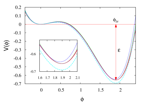
Figure 1: The effective potential for $\alpha=0.7$ and $\beta=0.3$. solid line: tree level potential; dotted line: case $I$; dash-dotted line: case $II$; short-dashed line: case $III$; long-dashed line: case $IV$; cases $I$ and $III$ are hardly visible.

9.2 The bounce profiles

In the semiclassical approximation the profiles $\phi(r)$ are, at fixed parameter $\alpha$ and arbitrary values of $\beta$, determined by one universal profile

$$\hat{\phi}_{\alpha}(r)=\beta^{-1/2}\phi(r)$$ (9.4)

which is independent of $\beta$. Therefore, the change of the profile by the back-reaction can be displayed in a transparent way by plotting, at fixed $\alpha$, the corresponding normalized profiles

$$\hat{\phi}(r)=\beta^{-1/2}\phi(r)$$ (9.5)

for different values of the parameter $\beta$. For large $\beta$, when the backreaction is weak, these profiles are expected to be independent of $\beta$ and close to $\hat{\phi}_{\alpha}(r)$. Indeed this is what we observe for $\beta\gtrsim 10$. The $\beta$-dependence observed for smaller values of $\beta$ depends on the type of back-reaction and on the renormalization conditions. For the presentation in Fig. 2 we have chosen the Hartree approximation and the renormalization conditions which preserve the position of the true vacuum (case $III$). With decreasing $\beta$ the normalized profiles get lower and lower in the central region of the bounce. If $\beta$ becomes smaller than $1$, this decrease becomes substantial. For some lower limiting value of $\beta\simeq 0.2$ the iterative procedure ceases to converge, during the iteration the profile collapses to $\phi(r)\equiv 0$. The qualitative behavior is similar for all other cases and all parameters $\alpha$ we have considered ($0.2,0.3,\dots 0.8$).

Figure 2: Behavior of $\hat{\phi}(r)=\phi(r)/\sqrt{\beta}$ for $\beta=20,1,0.5,0.25$ and $0.2$ at $\alpha=0.6$, for case III. In the central region, $r\lesssim 4$ these profiles are seen to decrease with decreasing $\beta$ while they are independent of $\beta$ in the semiclassical approximation.

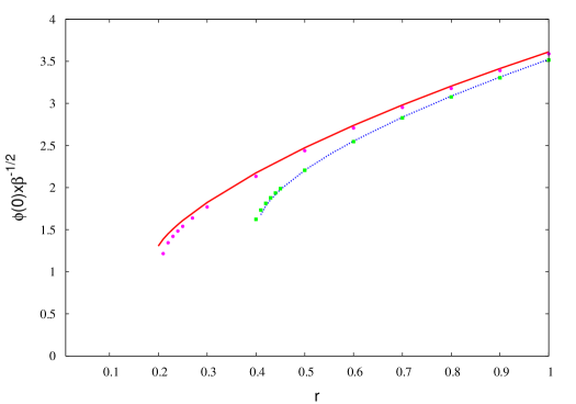
Figure 3: Behavior of $\phi(0)/\sqrt{\beta}$ near the critical values which limit the region of convergence for $\alpha=0.6$. Short-dashed line: case $I$; full squares: case $II$; solid line: case $III$ and full circles: case $IV$.

In Fig. 3 we show the behavior of $\phi(0)/\sqrt{\beta}$ near the critical values of $\beta$ for the four different cases. This ratio becomes constant as $\beta\to\infty$ and would be constant throughout in the semiclassical approximation. The behavior near the critical values is seen to be singular, as far as one can tell from a numerical computation. We therefore think that this phenomenon is genuine and not related to the way in which we iterate the equations. We have tried to modify the iteration by using the standard “overrelaxation” scheme

$$f_{i+1}(r)=\sigma f_{i}(r)+(1-\sigma)({\cal O}f_{i})(r)$$ (9.6)

where $f_{i}(r)$ is the $i$’th iteration of $\phi(r)$ and ${\cal M}(r)$, and ${\cal O}$ is the operation that generates the new profiles in the normal iterative process ($\sigma=0$). The runaway of the iteration below the critical value of $\beta$ was persistent for various parameters $\sigma$ that we have tried out. The tendency towards $\phi\equiv 0$ is apparent already for the parameter values of $\beta$ where the iteration still converges, see Fig. 2.

For $\alpha\lesssim 0.6$ and Hartree back-reaction the critical values of $\beta$ are around $\beta\simeq 0.2$ and then increase strongly. For the one-loop backreaction they increase roughly linearly from $0.2$ to $0.6$ between $\alpha=0.3$ and $\alpha=0.7$. At $\alpha=0.8$ the critical value is around $\beta=6$ (!) for all cases.

9.3 Effective actions and transition rates

As mentioned above, the effective action in the semiclassical case is of the form

$$S_{\rm eff}=\beta\hat{S}_{\rm cl}[\hat{\phi}]+S_{1-\rm loop}\;,$$ (9.7)

where $\hat{S}_{\rm cl}$ and $S_{1-\rm loop}$ are functions of $\alpha$ only. So we may display the effect of the back-reaction by plotting

$$\rho=\frac{S_{\rm eff}}{\beta\hat{S}_{\rm cl}[\hat{\phi}]+S_{1-\rm loop}}\;,$$ (9.8)

where $S_{\rm eff}$ is the effective action in the various approximations and renormalization conventions. $S_{1-\rm loop}$ in the denominators depends on the renormalization and is therefore different in the various cases. Clearly the ratio $\rho$ should go to unity as $\beta\to\infty$, because there $\eta=1/2\sqrt{\beta}$ and $\lambda=\alpha/\beta$ go to zero. Actually already for $\beta\gtrsim 1$ $\rho$ is very close to one. Even near the point where the iteration ceases to converge, the deviation from unity is only a few percent.

We display $\rho$ in Figs. 4 and Figs. 5. Both figures show the deviations for the four different cases. We see that the deviations for $\beta\gtrsim 1$ are quite small; for $\beta=0.3$ $\rho$ is larger than $1$ for all $4$ cases, for $\beta=0.6$ we have $\rho<1$ for $\beta>0.5$, for smaller values it increases strongly and displays some singlarity, a cusp or pole, near the critical value. The semiclassical action is dominated by the classical action, and so is the effective action including the various backreactions. We have, e.g., for $\alpha=0.6$ and case II, $S_{\rm semi-cl}=395.08\beta-29.522$ where the first term is the classical action, and the second one the one-loop action. So the contribution of the quantum action is relatively small, and even substantial changes would not affect $\rho$. Indeed near the critical point it is the classical action which deviates strongly from its semiclassical value, and this is due to the strong changes in the profile $\phi(r)$. We have to stress that here we are considering relative changes of the effective action. As the effective actions are of the order of a few hundred this implies absolute changes of several units, and this is what enters the transition rates.

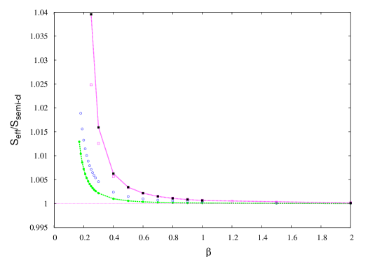
Figure 4: Ratio of $S_{\rm eff}$ and $S_{\rm semi-cl}$ as a function of $\beta$ for $\alpha=0.3$; dotted line with full squares: case I; empty squares: case II; long-dashed line with full circles: case III; empty circles: case IV.

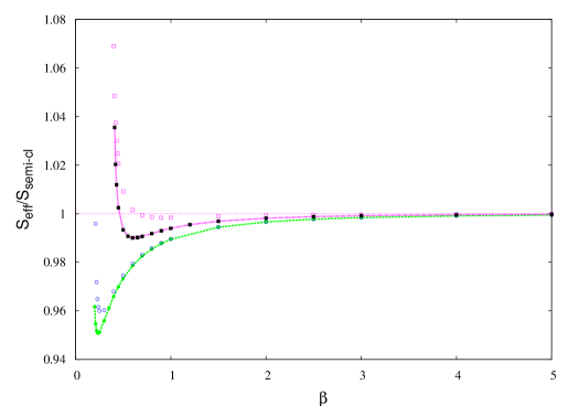
Figure 5: Ratio of $S_{\rm eff}$ and $S_{\rm semi-cl}$ as a function of $\beta$ for $\alpha=0.6$; dotted line with full squares: case I; empty squares: case II; long-dashed line with full circles: case III; empty circles: case IV.

Another quantity of interest is, therefore, the ratio between the transition rates and their semiclassical values. In part this reflects the behavior of the effective actions, but also includes the ratio of the prefactors. For large $\beta$ these ratios will again go to unity, the logarithm will go to zero. We plot the logarithm of $\Gamma/\Gamma_{\rm semi-cl}$ for small values of $\beta$, for $\alpha=0.3$ and $\alpha=0.6$. We see that the ratio can amount to several orders in magnitude. for the one-loop backreaction. the rates are always suppressed with respect to the semiclassical rate. This is what we found as well in the $2$-dimensional case [18] for the Hartree backreaction. Here we find, for the Hartree case, suppression for $\beta\lesssim 0.5$ and enhancement for larger values of $\alpha$.

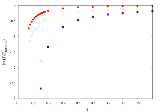
Figure 6: Logarithm of the ratio $\Gamma/\Gamma_{\rm semi-cl}$ as a function of $\beta$ for $\alpha=0.3$; full squares: case I; empty squares: case II; full circles: case III; empty circles: case IV.

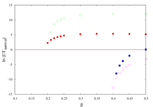
Figure 7: Logarithm of the ratio $\Gamma/\Gamma_{\rm semi-cl}$ as a function of $\beta$ for $\alpha=0.6$; full squares: case I; empty squares: case II; full circles: case III; empty circles: case IV.

We have not been able to pinpoint precisely the reason for disappearance of the bounce solution at small $\beta$. We can add the following comments:

• the fluctuation integral shows no anomaly in the critical region. This means in particular that the instability of the classical solution is not caused by the appearance of a further unstable mode in the fluctuation operator. If the squared frequency of such a mode would cross zero, the fluctuation integral would receive a very large contribution proportional to the square of its wave function. We display the fluctuation integral $\alpha=0.5$ and for various values of $\beta$ in Fig. 8. In the semiclassical approximation it is independent of $\beta$, here we clearly see a $\beta$-dependence which becomes stronger for small $\beta$, but there is no sign of a singularity in this behaviour near the critical value $\beta\simeq 0.2$. In the equation of motion for $\phi$ this integral is multiplied by $\lambda\phi=\alpha\phi/\beta$, so this contribution becomes more and more important for small $\beta$.

  

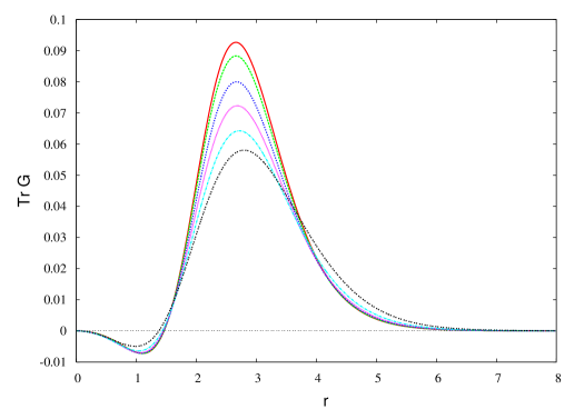
  Figure 8: The fluctuation integral ${\cal F}(r)$ for the Hartree backreaction, case $III$, as a function of $r$ for $\alpha=0.5$. The curves display a decrease with $\beta$, which takes the values $10,2.5,0.9,0.5,0.3$ and $0.2$.

• the deviations of $S_{\rm eff}$ from the semiclassical action are mostly due to the changes in the classical action, induced by the change of the profiles $\phi(r)$. The one-loop and double-bubble contributions to the effective action do change substantially, but their influence on $S_{\rm eff}$ remains numerically small.

• the convergence of the partial wave summation both for the fluctuation determinant and for the fluctuation integral is very good; we have included terms up to $n=20$ and included the asymptotic tail by an extrapolation (see Refs. [10, 18]). The convergence remains excellent near the critical values of $\beta$.

• we have not spent too much effort in studying the region $\alpha>0.7$, where we approach the thin-wall regime. The classical actions become so large there that the semiclassical action is of the order of a few thousands (e.g. $1500\beta$ for $\alpha=0.8$) and correspondingly the transition rates are incredibly small. We note, nevertheless, that for $\alpha=0.8$ the critical values of $\beta$ are around $6$ in the various cases we have studied.

We think that the instability of the bounce solution is mainly due to the term $\lambda\phi(r){\cal F}(r)$ in the differential equation for the bounce. Its effects are difficult to analyze: we do not simply have a change of the effective potential, as displayed in Fig. 1, but a modification that depends on $r$.

10 Summary and conclusions

We have presented here two schemes for incorporating quantum backreaction into the computation of transition rates in quantum field theory, here applied to false vacuum decay via a bounce: a one-loop backreaction, where the bounce profile is computed so as to minimize the effective action instead of the classical action; and the Hartree backreaction where the quantum backreaction is included into the computation of the profile and of the quantum fluctuations. We have derived the general equations including their finite, renormalized form. We have used dimensional regularization and applied two different sets of renormalization conditions.

We have presented numerical results for different parameter sets, using the $\alpha-\beta$ parametrization of Ref. [32]. The corrections to the semiclassical transition rate remain small as long as $\beta=1/4\eta^{2}$ is greater than $0.6$ and $\alpha=\lambda\beta$ is smaller than $0.7$. For lower values of $\beta$ the deviations from the semiclassical transition rate become sizeable and can amount to several orders of magnitude. These deviations depend on the approximation, one-loop or Hartree, and on the renormalization conditions. The transition rates are reduced for the one-loop backreaction, for the Hartree backreaction they are reduced for $\alpha\lesssim 0.5$ and enhanced for larger values of $\alpha$.

We find a critical value of $\beta$, below which our iteration ceases to converge. The behavior of various quantities near this value suggests that this is a genuine phenomenon and not a technical deficiency of our iteration scheme. If this is so, it implies that bounce solutions do not exist below this critical value and that in this region the false vacuum decay proceeds via different configurations in functional space. This is not unexpected for strong couplings: $\eta\gtrsim 1$ and $\lambda\gtrsim\alpha/0.3$.

Clearly, the computation of transition rates using the semiclassical approximation and with quantum backreaction remain approximations which cannot be compared, at present, with experimental results or with lattice computations, such as those in Refs. [33, 34, 35]. So it is not clear to what extent the inclusion of one-loop corrections, with or without backreaction, really represents an improvement. We may infer from our results that the semiclassical approximation is stable with respect to these higher corrections for $\alpha\lesssim 0.7$ and $\beta\gtrsim 0.6$, so we may believe it to be reliable. For lower values of $\beta$ the deviations are strong, especially in the transition rates they amount to a few orders of magnitude. As the different approximations lead to quite different results, a comparison with lattice data would be of great interest.

The methods presented here can be applied to various other computations of quantum backreaction, e.g. to the selfconsistent computation of classical solutions which minimize the sum of classical and zero point energies. While there one does not use the determinant theorem, one likewise employs techniques based on Green’s functions in Euclidean space [25, 36, 37] or techniques based on the analysis of phase shifts [38, 39, 40]. Other possible applications of such selfconsistent computations include quantum corrections to instantons [13, 41], vortices [42, 43, 44] and other classical solutions in quantum field theory. There are even cases without such a classical solution as, e.g., the selfconsistent pion cloud in the chiral quark model [45, 46, 47, 36].

Appendix A Renormalization of the effective potential

A.1 The one-loop effective potential

In the one-loop approximation the Green’s function are computed with the effective mass

$${\cal M}^{2}=U^{\prime\prime}(\phi)=m^{2}-6\eta\phi+\frac{3}{2}\lambda\phi^{2}\;.$$ (A.1)

Including the classical potential and the counterterms the 1-loop effective potential is given by

$$U_{\rm eff}(\phi) = U(\phi)+\frac{1}{2}\ln\det\frac{-\partial^{2}+{\cal M}^{2}}{-\partial^{2}+m^{2}}+\delta U(\phi)$$

$$= \frac{m^{2}}{2}\phi^{2}-\eta\phi^{3}+\frac{\lambda}{8}\phi^{4}-\frac{{\cal M}^{4}}{64\pi^{2}}\left(L_{\epsilon}-\ln\frac{{\cal M}^{2}}{m^{2}}+\frac{3}{2}\right)+\frac{m^{4}}{64\pi^{2}}\left(L_{\epsilon}+\frac{3}{2}\right)$$

$$+\delta\rho\phi+\frac{1}{2}\delta m^{2}\phi^{2}-\delta\eta\phi^{3}+\frac{1}{8}\delta\lambda\phi^{4}$$

$$\;.$$ (A.2)

For the first and the second derivative of effective potential one finds

$$U_{\rm eff}^{\prime}(\phi) = m^{2}\phi-3\eta\phi^{2}+\frac{\lambda}{2}\phi^{3}+\delta\rho+\delta m^{2}\phi-3\delta\eta\phi^{2}$$

$$- \frac{{\cal M}^{2}}{32\pi^{2}}(3\lambda\phi-6\eta)\left(L_{\epsilon}-\ln\frac{{\cal M}^{2}}{m^{2}}+1\right)\;,$$

$$U_{\rm eff}^{\prime\prime}(\phi) = m^{2}-6\eta\phi+\frac{3}{2}\lambda\phi^{2}+\delta m^{2}-6\delta\eta\phi+\frac{3}{2}\delta\lambda\phi^{2}$$

$$- \frac{1}{32\pi^{2}}(3\lambda\phi-6\eta)^{2}\left(L_{\epsilon}-\ln\frac{{\cal M}^{2}}{m^{2}}\right)-\frac{3\lambda{\cal M}^{2}}{32\pi^{2}}\left(L_{\epsilon}-\ln\frac{{\cal M}^{2}}{m^{2}}+1\right)\;.$$

We have already $U_{\rm eff}(0)=0$. The vanishing of the first derivative at $\phi=0$ fixes

$$\delta\rho=-\frac{12\eta m^{2}}{64\pi^{2}}(L_{\epsilon}+1)\;.$$ (A.5)

The condition $U^{\prime\prime}(0)=m^{2}$ leads to

$$\delta m^{2}=\frac{3}{32\pi^{2}}(12\eta^{2}+\lambda m^{2})L_{\epsilon}+\frac{3\lambda m^{2}}{32\pi^{2}}\;.$$ (A.6)

The absolute minimum (true vacuum) of the classical potential occurs at

$$\phi_{\rm tv}=\frac{3\eta}{\lambda}+\sqrt{\frac{9\eta^{2}}{\lambda^{2}}-\frac{2m^{2}}{\lambda}}\;.$$ (A.7)

If its position (the vacuum expectation value) is to be retained we have to require $U^{\prime}_{\rm eff}(\phi_{\rm tv})=0$. If the energy difference $\epsilon$ between the vacua is put equal to its tree level value we have to impose

$$U_{\rm eff}(\phi_{\rm tv})=U(\phi_{\rm tv})\;.$$ (A.8)

The latter two conditions lead to

$$\delta\eta = 9\eta\lambda\frac{L_{\epsilon}}{32\pi^{2}}+\delta\eta_{\rm fin}\;,$$ (A.9)

$$\delta\lambda = \frac{9\lambda^{2}}{32\pi^{2}}L_{\epsilon}+\delta\lambda_{\rm fin}\;,$$ (A.10)

where the finite parts satisfy the linear system of equations

$$-\delta\eta_{\rm fin}\phi_{\rm tv}^{3}+\frac{1}{8}\delta\lambda_{\rm fin}\phi_{\rm tv}^{4}$$ (A.11)

$$=\frac{1}{64\pi^{2}}\left[-{\cal M}_{\rm tv}^{4}\left(\ln\frac{{\cal M}_{\rm tv}^{2}}{m^{2}}-\frac{3}{2}\right)-3\lambda m^{2}\phi^{2}_{\rm tv}+12\eta m^{2}\phi_{\rm tv}-\frac{3}{2}m^{4}\right]\;,$$

$$-3\delta\eta_{\rm fin}m^{2}\phi_{\rm tv}^{2}+\frac{1}{2}\delta\lambda_{\rm fin}\phi_{\rm tv}^{3}$$ (A.12)

$$=\frac{6\lambda\phi_{\rm tv}-12\eta}{64\pi^{2}}\left[-{\cal M}_{\rm tv}^{2}(\ln\frac{{\cal M}_{\rm tv}^{2}}{m^{2}}-1)-m^{2}\right]\;,$$

with ${\cal M}^{2}_{\rm tv}={\cal M}^{2}(\phi_{\rm tv})$.

A.2 The Hartree effective potential

In the Hartree approximation the self-consistent effective potential as a function of $\phi$ is obtained from a variational potential

$${\cal U}(\phi,{\cal M}^{2}) = U(\phi)+\frac{1}{2}\ln\det\frac{-\partial^{2}+{\cal M}^{2}}{-\partial+m^{2}}-\frac{3\lambda}{8}\Delta^{2}+\delta U_{\rm div}+\delta U_{\rm fin}(\phi)$$ (A.13)

$$= \Lambda_{\rm fin}+\delta\rho_{\rm fin}\phi+\frac{m^{2}+\delta m^{2}_{\rm fin}}{2}\phi^{2}-(\eta+\delta\eta_{\rm fin})\phi^{3}+\frac{\lambda+\delta\lambda_{\rm fin}}{8}\phi^{4}$$

$$-\frac{{\cal M}^{4}}{64\pi^{2}}\left(L_{\epsilon}-\ln\frac{{\cal M}^{2}}{m^{2}}+\frac{3}{2}\right)+\frac{m^{4}}{64\pi^{2}}\left(L_{\epsilon}+\frac{3}{2}\right)-\frac{3\lambda}{8}\Delta^{2}$$

$$+\Lambda_{\rm div}+B{\cal M}^{4}\;,$$

with

$$\Delta(\phi,{\cal M}^{2})=\frac{2}{3\lambda}\left({\cal M}^{2}-m^{2}-\delta m^{2}_{\rm fin}+6(\eta+\delta\eta_{\rm fin})\phi-\frac{3}{2}(\lambda+\delta\lambda_{\rm fin})\phi^{2}\right)\;,$$ (A.14)

by the condition

$$\partial{\cal U}(\phi,{\cal M}^{2})/\partial{\cal M}^{2}=0\;.$$ (A.15)

The extremum is a maximum, so one has

$$U_{\rm eff}(\phi)=\max_{{\cal M}^{2}}~{}{\cal U}(\phi,{\cal M}^{2})\;.$$ (A.16)

The condition (A.15) yields the gap equation

$${\cal M}^{2} = m^{2}+\delta m^{2}_{\rm fin}-6(\eta+\delta\eta_{\rm fin})\phi+\frac{3}{2}(\lambda+\delta\lambda_{\rm fin})\phi^{2}$$ (A.17)

$$+\frac{3}{2}\lambda\left[-\frac{{\cal M}^{2}}{16\pi^{2}}\left(L_{\epsilon}-\ln\frac{{\cal M}^{2}}{m^{2}}+1\right)+4B{\cal M}^{2}\right]\;,$$

so that

$$\Delta=-\frac{{\cal M}^{2}}{16\pi^{2}}\left(L_{\epsilon}-\ln\frac{{\cal M}^{2}}{m^{2}}+1\right)+4B{\cal M}^{2}\;.$$ (A.18)

Nevertheless, for the variation of the potential ${\cal U}(\phi,{\cal M}^{2})$ of Eq. (A.13), $\Delta$ is defined as in Eq. (A.14), i.e., as a function of $\phi$ and ${\cal M}^{2}$. Cancellation of divergences in the gap equation requires $B=L_{\epsilon}/64\pi^{2}$ up to finite terms. It is convenient to choose

$$B=\frac{L_{\epsilon}+1}{64\pi^{2}}\;.$$ (A.19)

Cancellation of divergences in the effective action then entails

$$\Lambda_{\rm div}=-Bm^{4}=-\frac{L_{\epsilon}+1}{64\pi^{2}}m^{4}\;,$$ (A.20)

and we have

$$\Delta=\frac{{\cal M}^{2}}{16\pi^{2}}\ln\frac{{\cal M}^{2}}{m^{2}}\;,$$ (A.21)

so that $\Delta(0,{\cal M}^{2}(0))=\Delta(0,m^{2})=0$. If we want to impose, at $\phi=0$, the condition ${\cal M}^{2}(0)=m^{2}$ we obtain

$$\delta m^{2}_{\rm fin}=0\;.$$ (A.22)

The condition $U_{\rm eff}(0)=0$ fixes the finite cosmological constant to

$$\Lambda_{\rm fin}=\frac{3\lambda}{8}\Delta^{2}(0,m^{2})=0\;.$$ (A.23)

We now consider the first derivative of the effective potential. It is given by

$$U^{\prime}_{\rm eff}(\phi)=\frac{dU_{eff}(\phi)}{d\phi}=\frac{\partial{\cal U}(\phi,{\cal M}^{2})}{\partial\phi}+\frac{\partial{\cal U}(\phi,{\cal M}^{2})}{\partial{\cal M}^{2}}\frac{d{\cal M}^{2}}{d\phi}\;,$$ (A.24)

with ${\cal M}^{2}$ taken as the solution of the gap equation. Thereby the second term vanishes and so

$$U^{\prime}_{\rm eff}(\phi) = \delta\rho_{\rm fin}+m^{2}\phi-3(\eta+\delta\eta_{\rm fin})\phi^{2}+\frac{\lambda+\delta\lambda_{\rm fin}}{2}\phi^{3}$$

$$-\frac{1}{2}\left[6(\eta+\delta\eta_{\rm fin})-3(\lambda+\delta\lambda_{\rm fin})\phi\right]\Delta(\phi,{\cal M}^{2})\;.$$

The requirement $U^{\prime}_{\rm eff}(0)=0$, together with the condition ${\cal M}^{2}(0)=m^{2}$ then leads to

$$\delta\rho_{\rm fin}=3(\eta+\delta\eta_{\rm fin})\Delta(0,m^{2})=0\;.$$ (A.26)

With the present choice of the finite renormalizations we have

$$U_{\rm eff}(\phi)=\frac{m^{2}}{2}\phi^{2}-(\eta+\delta\eta_{\rm fin})\phi^{3}+\frac{\lambda+\delta\lambda_{\rm fin}}{8}\phi^{4}+\frac{{\cal M}^{4}}{64\pi^{2}}\left(\ln\frac{{\cal M}^{2}}{m^{2}}-\frac{1}{2}\right)+\frac{m^{4}}{128\pi^{2}}-\frac{3\lambda}{8}\Delta^{2}\;,$$ (A.27)

and

$$U^{\prime}_{\rm eff}(\phi)=m^{2}\phi-3(\eta+\delta\eta_{\rm fin})\phi^{2}+\frac{\lambda+\delta\lambda_{\rm fin}}{2}\phi^{3}-\frac{1}{2}\left[6(\eta+\delta\eta_{\rm fin})-3(\lambda+\delta\lambda_{\rm fin})\phi\right]\Delta\;.$$ (A.28)

The condition $U_{\rm eff}(\phi_{\rm tv})=U(\phi_{\rm tv})$ yields

$$\delta\eta_{\rm fin}\phi_{\rm tv}^{3}-\frac{\delta\lambda_{\rm fin}}{8}\phi_{\rm tv}^{4}=\frac{{\cal M}^{4}}{64\pi^{2}}\left(\ln\frac{{\cal M}^{2}}{m^{2}}-\frac{1}{2}\right)+\frac{m^{4}}{128\pi^{2}}-\frac{3\lambda}{8}\Delta^{2}\;,$$ (A.29)

and the condition $U^{\prime}_{\rm eff}(\phi_{\rm tv})=0$ leads to

$$3\delta\eta_{\rm fin}(\phi_{\rm tv}^{2}+\Delta)-\frac{\delta\lambda_{\rm fin}}{2}\phi_{\rm tv}(\phi_{\rm tv}^{2}+3\Delta)=-\frac{1}{2}\left[6\eta-3\lambda\phi_{\rm tv}\right]\Delta\;,$$ (A.30)

where in both equations ${\cal M}^{2}$ and $\Delta$ are taken at $\phi=\phi_{\rm tv}$. As $\delta\eta_{\rm fin}$ and $\delta\lambda_{\rm fin}$ appear in the equations for ${\cal M}^{2}$ and $\Delta$ we obtain a nonlinear system of equations for $\delta\eta_{\rm fin}$ and $\delta\lambda_{\rm fin}$. We have solved this system numerically using an iterative procedure.

In the $\overline{MS}$ scheme one generally lets $L_{\epsilon}\to 0$ and does not introduce any counterterms. Here we have to ensure that we have bare vacuum conditions at $\phi=0$ with ${\cal M}^{2}(0)=m^{2}$. This is obtained by setting $L_{\epsilon}+1\to 0$ and omitting all further counter terms. Then of course, as in the one-loop case with $\overline{MS}$ scheme, the minimum at $\phi_{\rm tv}$ is shifted away from its bare value.

Appendix B Renormalization of the effective action

B.1 Renormalization of the equation of motion 1-loop approximation

The equation of motion for the classical profile is given by

$$\phi^{\prime\prime}+\frac{3}{r}\phi^{\prime}-U^{\prime}(\phi)+\delta U^{\prime}(\phi)+\frac{1}{2}U^{\prime\prime\prime}(\phi){\cal F}=0\;.$$ (B.1)

The fluctuation integral is decomposed into the divergent leading order terms and a finite part as

$${\cal F}(x)={\cal F}^{(0)}(x)+{\cal F}^{(1)}(x)+{\cal F}^{\overline{(2)}}(x)\;.$$ (B.2)

The computation of the finite part ${\cal F}^{\overline{(2)}}$ has been described in section 5. The leading order parts are given analytically as

$${\cal F}^{(0)}(x)=\int\frac{d^{4}k}{(2\pi)^{4}}\frac{1}{k^{2}+m^{2}}=-\frac{m^{2}}{16\pi^{2}}\left(L_{\epsilon}+1\right)$$ (B.3)

and

$${\cal F}^{(1)}(x) = -\int d^{4}y\int\frac{d^{4}kd^{4}k^{\prime}}{(2\pi)^{8}}\frac{e^{i(k-k^{\prime})\cdot(x-y)}}{(k^{2}+m^{2})(k^{\prime 2}+m^{2})}V(y)$$ (B.4)

$$= -\int\frac{d^{4}k}{(2\pi)^{4}}\int\frac{d^{4}q}{(2\pi)^{4}}\frac{e^{iq\cdot x}\tilde{V}(q)}{(k^{2}+m^{2})((k+q)^{2}+m^{2})}\;,$$

where we have defined the Fourier transformation

$$\tilde{V}(q)=\int d^{4}ye^{-iq\cdot y}V(y)\;.$$ (B.5)

The integration over $k$ can be done and one obtains

$${\cal F}^{(1)}(x)=-\frac{1}{16\pi^{2}}L_{\epsilon}V(x)+{\cal F}^{(1)}_{\rm fin}(x)$$ (B.6)

with

$${\cal F}^{(1)}_{\rm fin}(x) = -\frac{1}{16\pi^{2}}\int\frac{d^{4}q}{(2\pi)^{4}}e^{iq\cdot x}\tilde{V}(q)$$

$$\times\left(2-\frac{\sqrt{|q|^{2}+4m^{2}}}{|q|}\ln\frac{\sqrt{|q|^{2}+4m^{2}}+|q|}{\sqrt{|q|^{2}+4m^{2}}-|q|}\right)\;.$$

As the integrands, except for the exponentials, depend only on the absolute values of $x$ and $q$ the Fourier transforms reduce to Fourier-Bessel transform, we have

$$\tilde{V}(q)\to\tilde{V}(|q|)=\frac{4\pi^{2}}{|q|}\int_{0}^{\infty}drr^{2}J_{1}(|q|r)V(r)\;.$$ (B.8)

and similarly for ${\cal F}^{(1)}(x)\to{\cal F}^{(1)}(r)$.

In the equation of motion the fluctuation term and the counterterm potential are now given by

$$\delta U^{\prime}(\phi)+\frac{1}{2}U^{\prime\prime\prime}(\phi){\cal F}=\delta\rho+\delta m^{2}\phi-3\delta\eta\phi^{2}+\frac{1}{2}\delta\lambda\phi^{3}$$

$$+ \frac{1}{2}(3\lambda\phi-6\eta)\Big{[}-\frac{m^{2}}{16\pi^{2}}(L_{\epsilon}+1)-(\frac{3}{2}\lambda\phi^{2}-6\eta\phi)\frac{1}{16\pi^{2}}L_{\epsilon}$$

$$+ {\cal F}^{(1)}_{\rm fin}+{\cal F}^{\overline{(2)}}\Big{]}\;.$$

With the counterterms determined in Appendix A the divergent terms cancel and we get the finite expression

$$\delta U^{\prime}(\phi)+\frac{1}{2}U^{\prime\prime\prime}(\phi){\cal F} = -3\delta\eta_{\rm fin}\phi^{2}+\frac{1}{2}\delta\lambda_{\rm fin}\phi^{3}$$

$$+\frac{1}{2}(3\lambda\phi-6\eta)\Big{[}{\cal F}^{(1)}_{\rm fin}+{\cal F}^{\overline{(2)}}\Big{]}\;.$$

B.2 Renormalization of the action in 1-loop approximation

The 1-loop part of the effective action is given by

$$S_{1-l}=\frac{1}{2}\ln{\cal D}\;.$$ (B.10)

The logarithm of the fluctuation determinant can be expanded with respect to powers in the external potential $V(x)$ as

$$\ln{\cal D}=\ln\frac{-\partial^{2}+U^{\prime\prime}(\phi)}{-\partial^{2}+U^{\prime\prime}(0)}=\sum_{N=1}^{\infty}\frac{(-1)^{N+1}}{N}A^{N}\;.$$ (B.11)

The first two terms in this expansion contain divergent parts. We write

$$\ln{\cal D}=A^{(1)}-\frac{1}{2}A^{(2)}+(\ln{\cal D})^{\overline{(3)}}$$ (B.12)

and now consider the first two terms separatly.

$$A^{(1)}=\int\frac{d^{4}k}{(2\pi)^{4}}\frac{1}{k^{2}+m^{2}}\int d^{4}xV(x)\;.$$ (B.13)

Using dimensional regularization we get

$$A^{(1)}=-\frac{m^{2}}{16\pi^{2}}L_{\epsilon}\int d^{4}xV(x)+A^{(1)}_{\rm fin}$$ (B.14)

with

$$A^{(1)}_{\rm fin}=-\frac{m^{2}}{16\pi^{2}}\int d^{4}xV(x)\;.$$ (B.15)

For $A^{(2)}$ we have

$$A^{(2)} = \int\frac{d^{4}k}{(2\pi)^{4}}\frac{d^{4}k^{\prime}}{(2\pi)^{4}}\frac{\int d^{4}xd^{4}y~{}e^{i(k-k^{\prime})\cdot(x-y)}V(x)V(y)}{(k^{2}+m^{2})(k^{\prime 2}+m^{2})}$$ (B.16)

$$= \frac{1}{16\pi^{2}}L_{\epsilon}\int d^{4}x(V(x))^{2}+A^{(2)}_{\rm fin}$$

with

$$A_{\rm fin}^{(2)}=\frac{1}{128\pi^{4}}\int_{0}^{\infty}q^{3}dq|\tilde{V}(q)|^{2}\left[2-\frac{\sqrt{q^{2}+4m^{2}}}{q}\ln\frac{\sqrt{q^{2}+4m^{2}}+q}{\sqrt{q^{2}+4m^{2}}-q}\right]\;.$$ (B.17)

With the counterterms determined in Appendix A the full one-loop action becomes

$$S_{\rm eff} = S_{\rm cl}+S_{\rm 1l}$$

$$= S_{\rm cl}+\frac{1}{2}\ln{\cal D}^{\overline{(3)}}+\int d^{4}x\left(-\delta\eta_{\rm fin}\phi^{3}+\frac{\delta\lambda_{\rm fin}}{8}\phi^{4}\right)-\frac{1}{4}A_{\rm fin}^{(2)}\;.$$

The subtracted logarithm of the fluctuation determinant is evaluated according to section 6. For $A_{\rm fin}^{(2)}$, as well as for ${\cal F}^{(1)}_{\rm fin}$, we have analytical expressions, their evaluation involves numerical Fourier-Bessel transforms like the one in Eq. (B.8).

B.3 Renormalization in the Hartree approximation

Using the counterterms of Appendix A.2 and the analysis of the fluctuation integral in Appendix B.1, the finite gap equation has the form :

$${\cal M}^{2}(x) = m^{2}-6(\eta+\delta\eta_{\rm fin})\phi(x)+\frac{3}{2}(\lambda+\delta\lambda_{\rm fin})\phi^{2}(x)$$ (B.19)

$$+\frac{3}{2}\lambda{\cal F}_{\rm fin}(x)$$

with

$${\cal F}_{\rm fin}(x)=\frac{{\cal M}^{2}-m^{2}}{16\pi^{2}}+{\cal F}^{(1)}(x)+{\cal F}^{\overline{(2)}}(x)\;.$$ (B.20)

The first term arises from ${\cal F}^{(0)}$ in Eq. (B.3), the divergent part of ${\cal F}^{(1)}$ in Eq. (B.6) and the counterterm $4B{\cal M}^{2}={\cal M}^{2}(L_{\epsilon}+1)/16\pi^{2}$ in the gap equation (A.17). Once the profile and the fluctuation integral have been computed Eqns. (B.19) and (B.20) determine ${\cal M}^{2}$. The finite equation of motion becomes

$$-\Delta_{4}\phi+U^{\prime}(\phi)+\delta U^{\prime}_{\rm fin}(\phi)-\frac{1}{2}(-6(\eta+\delta\eta_{\rm fin}+3(\lambda+\delta\lambda_{\rm fin}\phi){\cal F}_{\rm fin}=0\;.$$ (B.21)

In this case the action is given by

$$S_{\rm eff} = S_{\rm cl}+\delta S_{\rm fin}+\frac{1}{2}\ln{\cal D}^{\overline{(3)}}-\frac{1}{4}A^{(2)}_{\rm fin}+\frac{1}{64\pi^{2}}\int d^{4}xV^{2}(x)$$ (B.22)

$$- \frac{3}{8}\lambda\int d^{4}x{\cal F}_{\rm fin}^{2}$$

with

$$\delta S_{\rm fin}=\int d^{4}x\left[-\delta\eta_{\rm fin}\phi^{3}(x)+\frac{\delta\lambda_{\rm fin}}{8}\phi^{4}(x)\right]\;.$$ (B.23)

In the $\overline{MS}$ scheme all finite renormalizations are omitted in the gap equation, in the equation of motion and in the action, so that the latter reduces to

$$S_{\rm eff} = S_{\rm cl}+\frac{1}{2}\ln{\cal D}^{\overline{(3)}}-\frac{1}{4}A^{(2)}_{\rm fin}+\frac{1}{64\pi^{2}}\int d^{4}xV^{2}(x)$$ (B.24)

$$- \frac{3}{8}\lambda\int d^{4}x{\cal F}_{\rm fin}^{2}\;.$$

Of course the fluctuations in $\ln{\cal D}^{\overline{(3)}}$ and ${\cal F}_{\rm fin}$ and the potential $V(x)={\cal M}^{2}(x)-m^{2})$ are computed with a different ${\cal M}^{2}$ and the profiles in $A^{(2)}$ and in the classical action are computed using a different equation of motion.

References

- [1] S. R. Coleman, Phys. Rev. D15, 2929 (1977).
- [2] J. Callan, Curtis G. and S. R. Coleman, Phys. Rev. D16, 1762 (1977).
- [3] A. D. Linde, Nucl. Phys. B216, 421 (1983).
- [4] D. Cormier and R. Holman, Phys. Rev. D62, 023520 (2000), [hep-ph/9912483].
- [5] D. Cormier and R. Holman, Phys. Rev. D60, 041301 (1999), [hep-ph/9812476].
- [6] D. Boyanovsky, H. J. de Vega and R. Holman, hep-ph/9903534.
- [7] J. Garcia-Bellido, M. Garcia Perez and A. Gonzalez-Arroyo, Phys. Rev. D67, 103501 (2003), [hep-ph/0208228].
- [8] S. R. Coleman and F. De Luccia, Phys. Rev. D21, 3305 (1980).
- [9] J. C. Hackworth and E. J. Weinberg, Phys. Rev. D71, 044014 (2005), [hep-th/0410142].
- [10] J. Baacke and G. Lavrelashvili, Phys. Rev. D69, 025009 (2004), [hep-th/0307202].
- [11] J. Baacke and V. G. Kiselev, Phys. Rev. D48, 5648 (1993), [hep-ph/9308273].
- [12] G. V. Dunne and H. Min, Phys. Rev. D72, 125004 (2005), [hep-th/0511156].
- [13] J. Baacke and T. Daiber, Phys. Rev. D51, 795 (1995), [hep-th/9408010].
- [14] J. Baacke and S. Junker, Phys. Rev. D50, 4227 (1994), [hep-th/9402078].
- [15] J. Baacke and S. Junker, Phys. Rev. D49, 2055 (1994), [hep-ph/9308310].
- [16] A. Surig, Phys. Rev. D57, 5049 (1998), [hep-ph/9706259].
- [17] Y. Bergner and L. M. A. Bettencourt, Phys. Rev. D69, 045012 (2004), [hep-ph/0308107].
- [18] J. Baacke and N. Kevlishvili, Phys. Rev. D71, 025008 (2005), [hep-th/0411162].
- [19] S. Coleman, Aspects of Symmetry (Cambridge University Press, 1985).
- [20] M. Coppens and H. Verschelde, Z. Phys. C58, 319 (1993).
- [21] H. Verschelde and M. Coppens, Phys. Lett. B287, 133 (1992).
- [22] H. Verschelde, Phys. Lett. B497, 165 (2001), [hep-th/0009123].
- [23] E. Mottola, Phys. Rev. D 31, 754 (1985).
- [24] A. Erdelyi, editor, Higher Transcendental Functions (McGraw-Hill Book Company, Inc., New York, 1953).
- [25] J. Baacke, Z. Phys. C53, 402 (1992).
- [26] J. Baacke, Acta Phys. Polon. B22, 127 (1991).
- [27] R. F. Dashen, B. Hasslacher and A. Neveu, Phys. Rev. D10, 4114 (1974).
- [28] I. M. Gelfand and A. M. Yaglom, J. Math. Phys. 1, 48 (1960).
- [29] H. Verschelde and J. De Pessemier, Eur. Phys. J. C22, 771 (2002), [hep-th/0009241].
- [30] Y. Nemoto, K. Naito and M. Oka, Eur. Phys. J. A9, 245 (2000), [hep-ph/9911431].
- [31] J. Baacke and A. Heinen, Phys. Rev. D69, 083523 (2004), [hep-ph/0311282].
- [32] M. Dine, R. G. Leigh, P. Huet, A. D. Linde and D. A. Linde, Phys. Lett. B283, 319 (1992), [hep-ph/9203201].
- [33] M. G. Alford, H. Feldman and M. Gleiser, Phys. Rev. D47, 2168 (1993).
- [34] M. G. Alford and M. Gleiser, Phys. Rev. D48, 2838 (1993), [hep-ph/9304245].
- [35] G. D. Moore, K. Rummukainen and A. Tranberg, JHEP 04, 017 (2001), [hep-lat/0103036].
- [36] J. Baacke and H. Sprenger, Phys. Rev. D60, 054017 (1999), [hep-ph/9809428].
- [37] J. Baacke and H. Sprenger, Phys. Rev. D63, 094016 (2001), [hep-ph/0011204].
- [38] N. Graham et al., Phys. Lett. B572, 196 (2003), [hep-th/0207205].
- [39] N. Graham et al., Nucl. Phys. B645, 49 (2002), [hep-th/0207120].
- [40] N. Graham, R. L. Jaffe and H. Weigel, Int. J. Mod. Phys. A17, 846 (2002), [hep-th/0201148].
- [41] Y. Burnier and M. Shaposhnikov, Phys. Rev. D72, 065011 (2005), [hep-ph/0507130].
- [42] M. Goodband and M. Hindmarsh, Phys. Lett. B370, 29 (1996), [hep-ph/9510434].
- [43] M. Nagasawa and R. Brandenberger, Phys. Rev. D67, 043504 (2003), [hep-ph/0207246].
- [44] M. Bordag, Phys. Rev. D67, 065001 (2003), [hep-th/0211080].
- [45] D. Diakonov, V. Y. Petrov and P. V. Pobylitsa, Nucl. Phys. B306, 809 (1988).
- [46] C. V. Christov et al., Prog. Part. Nucl. Phys. 37, 91 (1996), [hep-ph/9604441].
- [47] R. Alkofer, H. Reinhardt and H. Weigel, Phys. Rept. 265, 139 (1996), [hep-ph/9501213].