Moduli Stabilization in Non-Geometric Backgrounds

hep-th/0611001 HUTP-06/A044

October 2006

1 Introduction

With the discovery of Calabi-Yau compactifications more than twenty years ago it became evident that many aspects of the 4D theory can be traced back to the topology of the internal manifold. It did not take long until backgrounds resembling the real world were constructed. At the same time it became evident that string theory does not have a unique ground state because the values of the moduli fields describing the deformations of the internal manifold could not be determined. This has been an open problem for many years, not only for particle phenomenology predictions coming from string theory, but also for string cosmology. This situation changed over the past years, as it has been realized that flux compactifications of string theory can stabilize all the moduli fields.

Due to the incorporation of fluxes, the continuous choice of moduli parameters was restricted to a large number of discrete choices. Thus this still left an extremely large number of string vacua. These vacua are part of the string theory landscape, which at present is analyzed with statistical methods [1] and techniques borrowed from number theory [3]. See [2] for a review.

All the more it is surprising that the number of explicit models known in the literature with all geometric moduli stabilized is rather limited [4] and no models leading to four-dimensional Minkowski space have been explicitly constructed. So far, moduli stabilization has been discussed in the literature in the supergravity approximation, a limit for which the radial modulus is assumed to be large and the string coupling is small. In many cases the radial modulus is then fixed in terms of non-perturbative corrections to the superpotential in a KKLT [5] like fashion, leading to supersymmetric Anti-de-Sitter vacua. More recently, moduli stabilization in terms of fluxes only (i.e. at the classical level) was achieved in [6] and in [7] in the context of type IIA massive supergravity, where it was shown that fluxes stabilize all geometric moduli of a simple $T^{6}/{\mathbb{Z}}_{3}\times{\mathbb{Z}}_{3}$ orientifold. In these models, the restrictions on the fluxes again result in a negative cosmological constant.

One of the goals of this paper is to construct a set of simple models in which all moduli are explicitly stabilized by fluxes only and which have a vanishing 4D cosmological constant. We will do so in the context of the type IIB theory, which allows the most freedom for dialing the fluxes. It is known that in this theory fluxes generate a classical superpotential for the complex structure moduli. This is in contrast to the potential for Kähler moduli, which is typically generated through non-perturbative effects, which are less under control.

To avoid the complication of stabilizing Kähler moduli, the basic idea underlying our work is to start in the type IIB theory with a model which does not have any Kähler moduli to begin with, and stabilize the complex structure moduli and the dilaton by turning on appropriate R-R and NS-NS fluxes. With ten-dimensional supergravity in mind, it appears quite hopeless to make any progress with this idea. Indeed, in any geometric compactification with an ordinary manifold $M^{6}$ as internal space, the overall size of that manifold will appear as a free parameter, a Kähler modulus. Thus, we will need $M^{6}$ to be non-geometric in one way or another. Thanks to string theory, we know that such non-geometric models do exist. It might be expected that the flux superpotential stabilizes all moduli in such compactifications and that the resulting supersymmetric vacua can be either Minkowski or AdS.

The fact that understanding string compactifications requires generalized notions of geometry is well-appreciated. The best-known example is probably the correspondence between sigma models on Calabi-Yau manifolds and an effective Landau-Ginzburg (LG) orbifold model as the “analytic continuation to small volume” of the sigma model [8, 9, 10]. This correspondence also plays a fundamental role in the understanding of mirror symmetry [11].

The existence of dualities has accentuated the relevance of string vacua without a ten-dimensional geometric interpretation. For instance, there are examples of Calabi-Yau manifolds whose complex structure cannot be deformed. Mirror symmetry exchanges the complex structure with the Kähler structure. Therefore, the mirror duals of such rigid manifolds would not have Kähler moduli and cannot correspond to a geometric manifold. Nevertheless, they have an effective world-sheet description as LG models, in accord with the general ideas of [11].

When turning on fluxes, mirror symmetry as well as other dualities require an even broader enlargement of the allowed class of compactification spaces. From the study of simple local or toroidal models, it is well-known that the mirror or T-duals of compactifications with generic fluxes cannot be described by a conventional geometry, see e.g., [13]. More generally, by looking at the panoply of R-R and NS-NS fluxes that are available in supergravity, and invoking (perturbative and non-perturbative) dualities, one can argue that the most general flux compactification will not allow a geometric description in any duality frame [14]. As mentioned above, the usual ten-dimensional effective supergravity of string theory will not be useful for the study of such vacua. Approaches which have been taken in the past include effective supergravity descriptions in dimensions less than ten dimensions [14, 15, 16], as well as exact world-sheet descriptions [14, 17, 18].

In the present paper, we will use a combination of “non-geometric” world-sheet techniques and 4D effective space-time description to exhibit a simple class of models in which all moduli can be stabilized by fluxes. Depending on the particular model, different values of the cosmological constant (Minkowski or AdS) are obtained. Charge conservation is accomplished by the presence of orientifolds.

We will illustrate such a generic claim in a precise manner, by studying two explicit models with Hodge numbers $h_{11}(M)=0$ and $h_{21}(M)=84$, $90$ respectively. The underlying models before turning on the fluxes are mirror duals of rigid Calabi-Yau manifolds and admit an effective description as LG models [12]. At a particular point in moduli space, they are also equivalent to some Gepner model [19].

Our models do not have a manifold interpretation, and therefore geometrical notions such as cycles, differential forms, etc., do not have the conventional meaning. An appropriate description of D-branes and supersymmetric cycles in LG models was developed in [20] using world-sheet techniques. A great deal of information about D-branes and orientifolds in Gepner models and their relation to LG and geometry is also available from the literature [21, 22, 23, 25, 26, 60]. For convenience we summarize the most important results in section 2.

The first new aspect of our work is the description of fluxes in these models, which is done in section 3. The flux configurations we are interested in satisfy constraints coming from supersymmetry and the type IIB tadpole cancellation condition. Supersymmetric type IIB vacua have fluxes belonging to the $H^{2,1}(M)\oplus H^{0,3}(M)$ cohomology of the internal space $M$. We will argue that these vacua are stable even non-perturbatively. This is due to the existence of a non-renormalization theorem for the superpotential of [27]. This basically follows because there are no relevant instantons to correct it. The existence of this non-renormalization theorem was crucial for the works [28, 29] where the classically generated superpotential (which is holographically dual to the sum of the planar diagrams of the gauge theory) does not receive any corrections. The fact that these results are in complete agreement with the exact non-perturbative dynamics of supersymmetric theories is a powerful check on the non-renormalization of the superpotential. We will also discuss in section 3 the other known consistency conditions of type IIB flux compactifications, including flux quantization and the tadpole cancellation condition.

In section 4, we will explicitly solve the supersymmetry equations which follow from the flux superpotential and the tadpole cancellation condition for the simpler of our two models, related to the so-called $1^{9}$ Gepner model. We find supersymmetric Minkowski vacua for several types of flux configurations.

It turns out that the spectrum of possibilities in the $1^{9}$ model is quite constrained, and we have not been able to find solutions leading to 4D AdS space in this model. One might ask whether this has any significance or whether it is just an accident in this particular case. We address this question in section 5 by repeating the analysis for the so-called $2^{6}$ Gepner model. We will see that the range of possibilities is much larger, and that we can in particular find 4D AdS solutions.

We would like to point out that we have not been able to find solutions or sequences of solutions in which the dilaton is stabilized at very small values, although we have no general argument why this cannot be done. Because of the non-renormalization theorem for the superpotential which we have mentioned above, having a string coupling of $O(1)$ does not affect the existence of the solutions. Nevertheless, it does mean that for other aspects of the solution, such as the masses of the moduli, as well as introduction of supersymmetry breaking effects which do receive quantum corrections, one should try to find a sequence of vacua which stabilize the coupling constant at weaker values.

In the appendix, we present an analysis of type IIB orientifolds of the quintic threefold from the LG point of view. In particular, we discuss the computation of the O-plane charge in the LG model, as well as the LG representation of the D3-brane sitting at a point of the quintic. The orientifold actions which we study include exchanges of variables, and have not been treated before in either the Gepner model or LG literature. This discussion, which is an application of the general setup of [26], serves as background for our discussion of tadpole cancellation condition in section 3.4.

We discuss the implications of our results for studies of the string theory landscape in section 6.

2 Branes and Orientifolds in Landau-Ginzburg models

Due to their simplicity, LG models of string compactifications have been studied in great detail over the years. They were among the first examples in which to access “stringy geometry”. Moreover, as studied in [8, 9, 10], LG models can often be thought of as the analytical continuation of Calabi-Yau sigma models to substringy volume.

The models for which this works most straightforwardly are Calabi-Yau hypersurfaces in weighted projective space. Namely, they are given by the vanishing locus of a homogeneous polynomial $P(x_{1},\ldots,x_{5})=0$ in five variables of weight $w_{1},\ldots,w_{5}$, and of total degree $H=\sum w_{i}$. Under the CY/LG correspondence, this sigma model corresponds to an ${\cal N}=(2,2)$ LG orbifold model with five chiral fields and world-sheet superpotential $W=P$. The orbifold group is a ${\mathbb{Z}}_{H}$ acting by phase rotations $x_{i}\to{\it e}^{2\pi{\it i}/h_{i}}x_{i}$, where $h_{i}=H/w_{i}$, which are assumed to be integer. For a special choice of polynomial $P$, this LG model flows in the IR to a particular CFT with a rational chiral algebra known as a Gepner model. These Gepner models are formally defined as the tensor product of some number $r$ of ${\cal N}=2$ minimal models of level $k_{i}=h_{i}-2$, such that the total central charge is $\hat{c}=\sum(1-2/h_{i})=3$. Gepner models with a hypersurface interpretation have $r=5$, in which case the central charge condition is equivalent to the CY condition on the degree of $P$.

The correspondence between LG models and Calabi-Yau sigma models can be extended to the boundary sector, D-branes, and orientifolds. Boundary states in Gepner models were first constructed in [21], and their geometric interpretation was first addressed in [22]. In [20], A-branes in LG models were shown to correspond to a particular type of non-compact cycle in the $x$-space on which the superpotential $W$ has a constant phase. More recently, B-branes in LG models were studied in terms of matrix factorizations [30]. For the extension to orientifolds, we refer to [23, 25, 26].

In the present paper, we will be concerned with a slightly different type of LG models which do not have a manifold interpretation, as we have mentioned in the introduction. Nevertheless, the techniques which are used to study LG models with such a connection can still be applied. Let us now proceed to introduce this technology concretely in the relevant examples, referring to the literature for the more general discussion.

2.1 The $1^{9}/{\mathbb{Z}}_{3}$ Gepner Model

2.1.1 Landau-Ginzburg model

Our first example is a LG model $M$ based on nine minimal models and world-sheet superpotential

$$W=\sum_{i=1}^{9}x_{i}^{3}\,,$$

divided by a ${\mathbb{Z}}_{3}$ generated by

$$g:x_{i}\to\omega x_{i},\quad i=1,2,\ldots 9\qquad\text{and}\qquad\omega\equiv{\it e}^{2\pi{\it i}/3}\,.$$ (2.1)

It is easy to compute the Hodge numbers of this model. As far as complex structure deformations are concerned, they all come from deformations of $W$ and a basis is given by the ${\mathbb{Z}}_{3}$-invariant monomials of the chiral ring ${\mathbb{C}}[x_{1},\ldots,x_{9}]/(x_{1}^{2},\ldots,x_{9}^{2})$. In other words they are given by the polynomials in the chiral fields

$$x_{i}x_{j}x_{k}\qquad{\rm with}\qquad i\neq j\neq k\neq i\,,$$ (2.2)

and there are $h_{2,1}(M)=84$ of them. To see that there are no Kähler structure deformations, we recall from [12] that ground states corresponding to the even cohomology always arise from the twisted sectors in LG orbifolds. In a ${\mathbb{Z}}_{3}$ orbifold, there are only two non-trivial twisted sectors, and the first must contribute to $h_{00}(M)=1$, while the second contributes in the conjugate $h_{33}(M)=1$. Hence $h_{11}(M)=h_{22}(M)=0$. This reasoning also readily implies that there are no contributions to $h_{21}(M)$ from the twisted sectors. As a result the Hodge diamond is

$$\begin{array}[]{cc}&1\\ &0~{}~{}~{}~{}~{}~{}0\\ &0~{}~{}~{}~{}~{}~{}0~{}~{}~{}~{}~{}~{}0\\ &1~{}~{}~{}~{}~{}84~{}~{}~{}~{}~{}84~{}~{}~{}~{}~{}1\\ &0~{}~{}~{}~{}~{}~{}0~{}~{}~{}~{}~{}~{}0\\ &0~{}~{}~{}~{}~{}~{}0\\ &1\\ \end{array}\,.$$ (2.3)

2.1.2 Geometric description

We can use the LG orbifold technology of [12] and the above-mentioned correspondence with geometry to give alternative descriptions of the background. To illustrate this idea consider the simpler example of the LG model based on the quotient of

$$W=x_{1}^{3}+x_{2}^{3}+x_{3}^{3}\,,$$ (2.4)

by a ${\mathbb{Z}}_{3}$ action which sends $(x_{1},x_{2},x_{3})\to\omega(x_{1},x_{2},x_{3})$. This corresponds to a $T^{2}$ torus model at the ${\mathbb{Z}}_{3}$ symmetric point in both complex structure and Kähler moduli space where

$$\tau=\omega\qquad{\rm and}\qquad\rho=\omega\,.$$ (2.5)

This model has three ${\mathbb{Z}}_{3}$ symmetries that will be relevant for us. Two of them act geometrically by phase rotations on the $x_{i}$’s, modulo the diagonal phase rotation which we have already divided out. These ${\mathbb{Z}}_{3}$’s correspond to geometric symmetries of the $T^{2}$. The third, somewhat less familiar, ${\mathbb{Z}}_{3}$ is a so-called “quantum symmetry” [12], and is formally identified with the dual of the original ${\mathbb{Z}}_{3}$ orbifold group defining our LG model,

$${\mathbb{Z}}_{3}^{\rm quantum}=({\mathbb{Z}}_{3}^{\rm LG})^{*}\cong{\mathbb{Z}}_{3}\,.$$ (2.6)

More concretely, the quantum symmetry multiplies a state in the $l$-th twisted sector by $\omega^{l}$. Dividing out by ${\mathbb{Z}}_{3}^{\rm quantum}$ gives back the unorbifolded LG model described by the polynomial (2.4).

The model $M$ of our interest is based on nine cubics instead of three, and it is natural to expect a relation to geometry via $(T^{2})^{3}=T^{6}$. The precise statement is that $M$ is mirror to a certain rigid Calabi-Yau $Z$ which can be obtained as a quotient of $T^{6}$ by a ${\mathbb{Z}}_{3}\times{\mathbb{Z}}_{3}$ action generated by

$$\begin{split}\tilde{g}_{12}:&\;(z_{1},z_{2},z_{3})\to(\omega z_{1},\omega^{-1}z_{2},z_{3})\,,\\ \tilde{g}_{23}:&\;(z_{1},z_{2},z_{3})\to(z_{1},\omega z_{2},\omega^{-1}z_{3})\,.\end{split}$$ (2.7)

Here $z_{1},z_{2},z_{3}$ are the complex coordinates of $T^{6}=(T^{2})^{3}$. This manifold has Hodge numbers $h_{11}(Z)=84$ and $h_{21}(Z)=0$. Note that in order for $\tilde{g}_{12},\tilde{g}_{23}$ to be symmetries, we have to fix the complex structure of the torus to be diagonal and equal to $\tau_{i}=\omega$ for $i=1,2,3$. Being mirror to $Z$, $M$ can also be described as a toroidal orbifold, except that the orbifold group does not act geometrically. To explain this in more detail, we state that $M$ can be obtained by starting from $T^{6}$, where now we fix the Kähler structure of $T^{6}$ at the ${\mathbb{Z}}_{3}$ orbifold point in each $T^{2}$ factor, $\rho_{i}=\omega$ for $i=1,2,3$, and divide out by a ${\mathbb{Z}}_{3}\times{\mathbb{Z}}_{3}$ subgroup of the $({\mathbb{Z}}_{3})^{3}$ quantum symmetry group. While preserving supersymmetry, this orbifold projects out all Kähler moduli, so that we end up with $h_{11}(M)=0$. The complex structure moduli of the torus are projected, and new ones appear in the twisted sector, for a total of $h_{21}(M)=84$.

Alternatively, we can start with the $1^{9}/{\mathbb{Z}}_{3}$ Gepner model and turn it into a $T^{6}$ at the orbifold point in Kähler moduli space by modding out by a ${\mathbb{Z}}_{3}\times{\mathbb{Z}}_{3}$ generated by

$$\begin{split}g_{1}:&\;(x_{1},x_{2},x_{3},x_{4},x_{5},x_{6},x_{7},x_{8},x_{9})\to(\omega x_{1},\omega x_{2},\omega x_{3},x_{4},x_{5},x_{6},x_{7},x_{8},x_{9})\,,\\ g_{2}:&\;(x_{1},x_{2},x_{3},x_{4},x_{5},x_{6},x_{7},x_{8},x_{9})\to(x_{1},x_{2},x_{3},\omega x_{4},\omega x_{5},\omega x_{6},x_{7},x_{8},x_{9})\,.\end{split}$$ (2.8)

The quantum symmetry group $({\mathbb{Z}}_{3})^{3}$ of this $W/({\mathbb{Z}}_{3})^{3}$ LG orbifold model of $(T^{2})^{3}$ is generated by $g_{1}^{*}$, $g_{2}^{*}$ and $g_{3}^{*}$, where $g_{3}=gg_{1}^{-1}g_{2}^{-1}$. The ${\mathbb{Z}}_{3}\times{\mathbb{Z}}_{3}$ which turns $T^{6}$ back into $M$ is then generated by $g_{1}^{*}(g_{2}^{*})^{-1}$ and $g_{2}^{*}(g_{3}^{*})^{-1}$, which are mirror duals of $\tilde{g}_{12}$ and $\tilde{g}_{23}$ in (2.7), respectively. Here, $g$ is the original orbifold generator in (2.1).

2.2 Orientifolds

2.2.1 Involutions

We intend to compactify type IIB string theory on an orientifold of $M$, which results in an ${\cal N}=1$ theory in four dimensions. The orientifold is defined by dividing out B-type world-sheet parity $\Omega_{B}$ dressed with a holomorphic involution $\sigma$ such that the square of it is in the orbifold group and such the superpotential is invariant up to a sign [23, 26]

$$W(\sigma x)=-W(x)\,.$$ (2.9)

This last condition comes from the fact that superpotential enters the world-sheet action as an F-term,

$$\int d\theta^{+}d\theta^{-}W(x)\,,$$ (2.10)

and B-type world-sheet parity exchanges the fermionic coordinates in superspace $\theta^{+}\leftrightarrow\theta^{-}$. The sign resulting from this parity transformation is compensated for by different types of involutions. The simplest involution that cancels the sign in (2.9) changes the sign of all nine bosonic coordinates

$$\sigma_{0}:\;(x_{1},x_{2},\ldots,x_{9})\to(-x_{1},-x_{2},\ldots,-x_{9})\,.$$ (2.11)

Under this transformation the superpotential changes sign $W(\sigma_{0}x)=-W(x)$. Since we are already working with a ${\mathbb{Z}}_{3}$ orbifold by $g$ in (2.1), we also have to divide out by the parity reversing symmetries $g\sigma_{0}$ and $g^{2}\sigma_{0}$. The full orientifold group ${\mathbb{Z}}_{3}\ltimes{\mathbb{Z}}_{2}\cong{\mathbb{Z}}_{6}$ is generated by $g\sigma_{0}$.

We can consider other orientifolds with a more non-trivial action on the $x_{i}$’s. In particular, we can permute, respectively, 1, 2, 3, or 4 pairs of $x_{i}$’s:

$$\begin{split}\sigma_{1}:\;(x_{1},x_{2},x_{3},x_{4},x_{5},x_{6},x_{7},x_{8},x_{9}),\to-(x_{2},x_{1},x_{3},x_{4},x_{5},x_{6},x_{7},x_{8},x_{9})\,,\\ \sigma_{2}:\;(x_{1},x_{2},x_{3},x_{4},x_{5},x_{6},x_{7},x_{8},x_{9})\to-(x_{2},x_{1},x_{4},x_{3},x_{5},x_{6},x_{7},x_{8},x_{9})\,,\\ \sigma_{3}:\;(x_{1},x_{2},x_{3},x_{4},x_{5},x_{6},x_{7},x_{8},x_{9})\to-(x_{2},x_{1},x_{4},x_{3},x_{6},x_{5},x_{7},x_{8},x_{9})\,,\\ \sigma_{4}:\;(x_{1},x_{2},x_{3},x_{4},x_{5},x_{6},x_{7},x_{8},x_{9})\to-(x_{2},x_{1},x_{4},x_{3},x_{6},x_{5},x_{8},x_{7},x_{9})\,.\end{split}$$ (2.12)

One of the effects of the orientifold is to project the space of complex structure deformations onto the subspace which is compatible with $W(\sigma x)=-W(x)$. The number of invariant complex structure deformations $h_{21}^{+}$, as well as invariant three-cycles, $b_{3}^{+}=2(h_{21}^{+}+1)$ is tabulated in table 1. They can be obtained as follows. The 84 deformations of $M$ correspond to the monomials $x_{i}x_{j}x_{k}$ with distinct $i,j,k=1,\ldots,9$. A parity $\sigma_{i}$ acts on these monomials, leaving $n_{\rm fix}(\sigma_{i})$ of them invariant up to the sign, and permuting the others pairwise. The number of (anti-)invariant deformations is then given by

$$h_{21}^{+}(M^{(\sigma_{i})})=\frac{84-n_{\rm fix}(\sigma_{i})}{2}+n_{\rm fix}(\sigma_{i})\,.$$ (2.13)

Eg, for $\sigma_{1}$, invariant monomials are $x_{1}x_{2}x_{j}$ with $j=3,\ldots,9$ as well as $x_{i}x_{j}x_{k}$ with distinct $i,j,k=3,\ldots,9$, so $n_{\rm fix}(\sigma_{1})=7+35=42$ and $h_{21}^{+}=63$.

orientifold	$h_{21}^{+}$	$b_{3}^{+}$
$\sigma_{0}$	84	170
$\sigma_{1}$	63	128
$\sigma_{2}$	52	106
$\sigma_{3}$	47	96
$\sigma_{4}$	44	90

Table 1: Number of invariant complex structure deformations for various orientifolds of $M$.

2.2.2 Orientifold planes

One important piece of data of an orientifold in the geometric setting is the fixed point locus of the involution that dresses world-sheet parity. The connected components of this fixed point locus are referred to as “orientifold planes” (O-planes). O-planes carry R-R charge and NS-NS tension. The crucial role of O-planes arises from the fact that both charge and tension can be negative, while preserving space-time supersymmetry. In fact, in compact models, O-planes are necessary in order to cancel the tadpoles generated by D-branes and fluxes.

In our present setup, which is non-geometric, there is no straightforward notion of orientifold “plane” as a geometric locus. Nevertheless, since the charge of O-planes can be detected on the world-sheet by computing a crosscap diagram with R-R field insertion, we can still ask in a meaningful way for the R-R charge sourced by the orientifold. We will present pertinent formulas for these R-R charges in subsection 2.4.

In geometric type IIB orientifolds, the mutually supersymmetric O-planes that can occur together are either O9 and O5-planes or O7 and O3-planes. In other words, the complex codimension of the fixed point locus of the dressing involution can be either $0\bmod 2$ or $1\bmod 2$. For example, we can view the type I string as a type IIB orientifold with trivial involution dressing world-sheet parity. This corresponds to the O9/O5-case, where O5-plane charge can be induced from the curvature of the compactification manifold.

In our model, we also have a similar distinction between two types of orientifolds based on the space-time supersymmetry of the crosscap state resulting from the various involutions. For instance, we can anticipate that the canonical action $\sigma_{0}$ corresponds to type I compactification on $M$. Then, because they are of “even codimension” in the sense of having an even number of $-1$ eigenvalues, the orientifolds associated with $\sigma_{2}$, and $\sigma_{4}$ are also of the O9/O5-type, and similarly $\sigma_{1}$ and $\sigma_{3}$ correspond to O7/O3-type. The latter is the class of orientifold models considered in the supergravity regime in [33], and in which moduli can be stabilized by fluxes. In this section, we will discuss all possible orientifolds of $M$. The fact that even in the non-geometric LG model we study we find only two distinct types of O-planes is a strong indication that even in the non-geometric model, the intuition of the geometric case continues to hold.

2.3 D-branes and supersymmetric cycles

2.3.1 Supersymmetric cycles

Before we can describe the fluxes and the tadpole cancellation condition in our model, we need to review some background material about the LG description of D-branes wrapping supersymmetric cycles. Generally speaking, there are two types of supersymmetric cycles in Calabi-Yau type compactifications: A-cycles are middle-dimensional cycles represented by (special) Lagrangian submanifolds. They are relevant for flux compactifications as the cycles supporting R-R and NS-NS three-form fluxes. B-cycles are even-dimensional cycles represented by holomorphic submanifolds carrying (stable) holomorphic vector bundles. They are the cycles that can be wrapped by O-planes and D-branes of various types to, for instance, support standard model gauge fields, cancel tadpoles from fluxes, etc.

In the non-geometric setting, the most useful way to talk about supersymmetric cycles is in terms of D-branes. Namely, we can distinguish A- and B-branes by the boundary conditions on the ${\cal N}=(2,2)$ supercurrents on the world-sheet

$$\begin{split}\text{A-type:}&\qquad\qquad G^{\pm}_{L}(z)=G^{\mp}_{R}(\bar{z})\quad\text{at}\quad\bar{z}=\bar{z}\,,\\ \text{B-type:}&\qquad\qquad G^{\pm}_{L}(z)=G^{\pm}_{R}(\bar{z})\quad\text{at}\quad z=\bar{z}\,.\end{split}$$ (2.14)

So let us review some of what is known about D-branes wrapping supersymmetric cycles in LG models. There are generally two languages to describe the cycles. In [20], A-branes in LG models were related to Picard-Lefshetz vanishing cycles of the singularity described by the LG superpotential. In the simple homogeneous cases, these cycles can be pictured as wedges in the $x$-plane, see e.g., Fig. 1. It is straightforward to implement orbifolding in this description. The other language we will use is the more abstract language of matrix factorizations, originally introduced in [30]. These matrix factorizations describe B-cycles in LG models and their orbifolds and have been studied extensively in the last few years.

Since A-model and B-model are mirror to each other, and the mirror of an LG model is an orbifold of it, we can also combine the roles of these two descriptions. The wedge description is easier to picture, while the matrix factorization approach is more general, in the sense that not all matrix factorizations have a (known) mirror wedge description. Moreover, the O-plane charge is in general only known how to compute in this language.

We will first describe these cycles in the parent LG model (including the orbifold, but before orientifolding). Later, we will describe how the orientifold projects them and work out invariant representatives.

2.3.2 A-branes

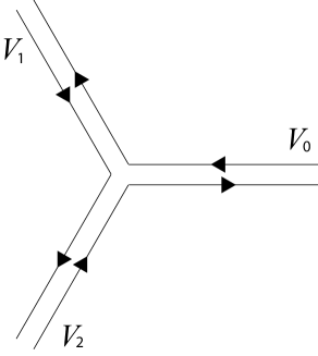
Figure 1: The piece of cake picture of Lagrangian (A-type) D-branes in LG model $x^{3}$.

By studying the A-type world-sheet supersymmetry condition (2.14), one finds [20] that A-type D-branes in LG models correspond to middle-dimensional cycles. In the $x$-space D-branes correspond to the preimages of the positive real axis (or, by an R-rotation, some other straight ray with constant slope) in the $W$-plane, i.e. to the preimages of

$${\rm Im}(W)=0\,.$$ (2.15)

In the simplest case of LG models, based on the superpotential $W=x^{k+2}$ (and its deformations), this condition can be solved completely, and one can compare with RCFT results on boundary states in ${\cal N}=2$ minimal models. Specifically, the condition (2.15) selects $(k+2)$ spokes through the origin in the $x$-plane at an angle which is an integer multiple of ${\it e}^{2\pi{\it i}/(k+2)}$, and the branes correspond to all possible wedges built from these spokes. A useful homology basis is provided by the $(k+2)$ wedges $V_{0},\ldots V_{k+1}$ of smallest angular size ${\it e}^{2\pi{\it i}/(k+2)}$.

For example, for the minimal model building block of the $1^{9}$ Gepner model, each of the factors comes with a set of three A-branes, see Fig. 1. We will call these three cycles $V_{0}$, $V_{1}$, and $V_{2}$. The $V_{n}$’s generate the homology of the minimal model, but satisfy the one relation

$$V_{0}+V_{1}+V_{2}=0\,,$$ (2.16)

as can be seen from the figure.

On the other hand, the cohomology basis of the space of A-type D-brane charges in the minimal model is spanned by the two R-R sector ground states, $|l\rangle$, with $l=1,2$ [12]. These can be equivalently represented by the chiral ring ${\mathbb{C}}[x]/x^{2}=\langle 1,x\rangle$. The correspondence is given by

$$|l\rangle\leftrightarrow x^{l-1}\,.$$ (2.17)

The R-R charges of the $V_{n}$’s can be computed as the overlaps [20] (disk one-point functions)

$$\langle V_{n}|l\rangle=\int_{V_{n}}x^{l-1}{\it e}^{-x^{3}}dx=(1-\omega^{l})\omega^{ln}\,.$$ (2.18)

The normalization we have chosen here differs slightly from the ones of [20], but is more convenient for our purposes.

2.3.3 Intersection form of A-cycles

For later applications, it is useful to discuss the action of the ${\mathbb{Z}}_{3}$ symmetry, as well as the intersection form on the A-cycles in the minimal model.

First of all, it is quite obvious that the ${\mathbb{Z}}_{3}$ symmetry which sends $x\to\omega x$ is represented on the $V_{i}$’s as

$$(V_{0},V_{1},V_{2})\to(V_{1},V_{2},V_{0})=(V_{0},V_{1},V_{2})g\qquad{\rm with}\qquad g=\begin{pmatrix}0&0&1\\ 1&0&0\\ 0&1&0\end{pmatrix}\,.$$ (2.19)

Turning to the intersection form, this is best defined as the Witten index ${\rm Tr}(-1)^{F}$ in the Hilbert space of open strings between two branes. Geometrically, there is clearly one R-R ground state localized at each geometric intersection point. In the more abstract setting such as the LG models considered herein, we can still compute ${\rm Tr}(-1)^{F}$ as the cylinder amplitude for open strings stretched between two branes with supersymmetric boundary conditions around the cylinder. In the limit that the cylinder becomes very long, this amplitude factorizes on disk amplitudes with closed string ground states inserted, thus providing an alternative (and often very simple) derivation of D-brane charges from the Witten index. In the case at hand, the intersection product between $V_{m}$ and $V_{n}$, which is defined as ${\rm Tr}_{{\cal H}_{mn}}(-1)^{F}$, follows most easily from the relation to soliton counting [20]. One finds

$${\rm Tr}_{{\cal H}_{mn}}(-1)^{F}={\rm id}-g=\begin{pmatrix}1&0&-1\\ -1&1&0\\ 0&-1&1\end{pmatrix}\,.$$ (2.20)

The “index theorem” which expresses this in terms of the R-R overlap (2.18) is explicitly

$${\rm Tr}_{{\cal H}_{mn}}(-1)^{F}=\frac{1}{3}\sum_{l=1,2}\langle V_{m}|l\rangle\frac{1}{1-\omega^{l}}\langle l|V_{n}\rangle\,,$$ (2.21)

where $\langle l|V_{n}\rangle=\overline{\langle V_{n}|l\rangle}$.

Clearly, (2.20) does not have full rank, which is a reflection of the relation in homology (2.16). We can truncate the ${\mathbb{Z}}_{3}$ representation and intersection matrix by passing to a basis of A-cycles, given for instance by $(V_{0},V_{1})$. The ${\mathbb{Z}}_{3}$ generator takes the form

$$A=\begin{pmatrix}0&-1\\ 1&-1\end{pmatrix}\,,$$ (2.22)

while the intersection matrix is

$$I=\begin{pmatrix}1&0\\ -1&1\end{pmatrix}\,.$$ (2.23)

We now tensor together nine such minimal models and orbifold by $g$ acting diagonally as in (2.1). The orbifolding projects R-R ground states and chiral ring to those states

$$|{\bf l}\rangle=|l_{1},\ldots,l_{9}\rangle\qquad{\rm with}\qquad l_{i}=1,2\qquad{\rm and}\qquad\sum_{i=1}^{9}l_{i}=0\bmod 3\,,$$ (2.24)

and identifies brane states by summing over orbits. We will denote these branes as

$$\Gamma_{[\bf n]}=\frac{1}{\sqrt{3}}(\otimes_{i}V_{n_{i}}+\otimes_{i}V_{n_{i}+1}+\otimes_{i}V_{n_{i}+2})\qquad{\rm with}\qquad{\bf n}=(n_{1},\ldots n_{9})\,,$$ (2.25)

where the $n_{i}$’s are taken $\bmod~{}3$. To see that the factor $1/\sqrt{3}$ on the RHS is the correct normalization factor of the boundary states, we look at the open string spectrum. Let us look in particular at the intersection index ${\rm Tr}(-1)^{F}$ between $\Gamma_{[\bf m]}$ and $\Gamma_{[\bf n]}$. In the parent (unorbifolded) LG model, each of them has three pre-images rotated by $g$. It is clear that the intersection of the two branes in the orbifold is given by looking at the intersection points of all these 9 preimages. Now if we rotate the preimages of both branes simultaneously, the intersection does not change, trivially because $g$ is a symmetry. In other words, the intersection points related by rotating both preimages simultaneously are gauge equivalent. Therefore, to obtain the intersection in the orbifold, we fix any one preimage of $\Gamma_{[\bf m]}$ and look for intersections with all preimages of $\Gamma_{[\bf n]}$. Thus, the intersection form on the $\Gamma_{[\bf n]}$ is given by [22]

$$(1-g)^{\otimes 9}\left[1+g^{\otimes 9}+(g^{\otimes 9})^{2}\right]\,,$$ (2.26)

or, restricted to those $\Gamma_{[\bf n]}$ with representatives with all $n_{i}=0,1$,

$${\bf I}=I^{\otimes 9}\left[1+A^{\otimes 9}+(A^{\otimes 9})^{2}\right]\,.$$ (2.27)

The same result can also be expressed in a form similar to (2.21)

$${\bf I}_{{\bf n}{\bf m}}=\frac{1}{3^{8}}\sum_{{\bf l}}\prod(1-\omega^{l_{i}})\frac{1}{\prod(1-\omega^{l_{i}})}\prod(1-\omega^{-l_{i}})\omega^{{\bf n}\cdot{\bf l}-{\bf m}\cdot{\bf l}}\,,$$ (2.28)

where ${\bf n}\cdot{\bf l}=\sum n_{i}l_{i}$ and the sum is over all ${\bf l}$ with $\sum l_{i}=0\bmod 3$, cf. (2.24). Since we are summing over $170$ intermediate states in (2.28), the $2^{9}\times 2^{9}$-dimensional matrix ${\bf I}$ has rank $\leq 170$. As it turns out, when restricting ${\bf I}$ to the first $170$ (in alphabetical order) of the $\Gamma_{[\bf n]}$ with $n_{i}=0,1$, ${\bf I}$ is invertible and has determinant $1$. We have thus described an algorithm for finding a minimal integral basis of A-cycles in our $1^{9}$ LG model.

2.3.4 B-branes and matrix factorization

The analog of (2.15) for B-type boundary condition (2.14) would naively impose the holomorphic condition $W=0$ at the boundary. Both conditions arise from the fact that the F-term world-sheet interaction $\int d^{2}\theta W$ is supersymmetric only up to partial integration, and picks up a contribution from the boundary if one is present. In the case of A-branes, this boundary term is eliminated by imposing the boundary condition (2.15). But for B-branes, restricting to $W=0$ would not allow for a great diversity of boundary conditions. In that case one introduces additional boundary degrees of freedom and boundary interactions whose susy variation will cancel the boundary term.

As it was shown in [30], one way of encoding these boundary interactions is in terms of matrix factorization. Briefly, a matrix factorization of the world-sheet superpotential $W$ is a block off-diagonal matrix $Q$ with polynomial entries in the LG variables and satisfying the equation

$$Q^{2}=W\cdot{\rm id}\,.$$ (2.29)

Physically, the boundary interactions encoded by $Q$ can be viewed as an open string tachyon configuration between space filling branes and anti-branes: The blocks of $Q$ correspond to the Chan-Paton spaces of the branes, resp., the anti-branes. The off-diagonal blocks correspond to the open string tachyon. The diagonal blocks could carry a gauge field configuration, which however can be gauge away in the standard LG models.

For example, for the minimal model $x^{3}$, there is essentially only one non-trivial factorization $x^{3}=x\cdot x^{2}$, with associated matrix factorization

$$Q=\begin{pmatrix}0&x\\ x^{2}&0\end{pmatrix}\qquad Q^{2}=x^{3}\cdot{\rm id}\,.$$ (2.30)

The spectrum of massless open strings between two such branes is computed as the cohomology of the matrix factorizations acting on matrices with polynomial entries. For the simple example (2.30) for instance, it is easy to see that there are exactly two such states,

$$\bigl{[}Q,\begin{pmatrix}1&0\\ 0&1\end{pmatrix}\bigr{]}=0,\qquad\bigl{\{}Q,\begin{pmatrix}0&1\\ -x&0\end{pmatrix}\bigr{\}}=0\,.$$ (2.31)

We must refer to the original literature [30], and citations thereof, for more details about the matrix factorization description of B-branes in minimal models. We will review the essentials here in view of their applications in our models.

Now let us discuss B-branes in orbifolds. The simplest, and also useful, example is the ${\mathbb{Z}}_{3}$ orbifold of a single minimal model $x^{3}$ divided by the action $x\to\omega x$. As we have mentioned, this orbifolding is nothing but an implementation of mirror symmetry, so we should compare the result with the wedge picture of A-branes in the (unorbifolded) model we have described above. Since we are dealing with space filling branes, we seek a representation of the orbifold group on their Chan-Paton spaces. It is easy to see that ${\mathbb{Z}}_{3}$-generator is represented on the matrix $Q$ of (2.30) by

$$\gamma=\omega^{n}\begin{pmatrix}1&0\\ 0&\omega\end{pmatrix}\,,$$ (2.32)

where $n=0,1,2$. This generator satisfies

$$\gamma Q(\omega x)\gamma^{-1}=Q(x)\,.$$ (2.33)

The factorization $Q$ equipped with these three representations of ${\mathbb{Z}}_{3}$ corresponds via mirror symmetry of the minimal model with its orbifold precisely to the three A-type wedges $V_{n}$ discussed in the previous subsection. One can also work out the projection on the open strings and thereby recover (2.20). The expressions (2.18) and (2.21) are then special cases of the general formulas in [31].

For our purposes, we are interested in the orbifold of $W=\sum_{i=1}^{9}x_{i}^{3}$ by a diagonal ${\mathbb{Z}}_{3}$. Before orbifolding, we have just one factorization, given by tensoring nine copies of $Q$ in (2.30). In the orbifold, this yields three different branes: We tensor together nine copies of $\gamma$ in (2.32), with naively $3^{9}$ choices of representation, but clearly only the sum of $n$’s ($\bmod 3$) matters. We’ll now call these three branes $\Lambda_{n}$, $n=0,1,2$. A different way to think of the $\Lambda_{n}$’s is as A-branes in the mirror $W/{\mathbb{Z}}_{3}^{8}$, where we are dividing by all symmetries that leave the product of $x_{i}$’s invariant. This orbifold action allows to “align” the wedges in all nine factors, so $\Lambda_{n}$ can be identified with $V_{n}$ in one of the factors, e.g., the first one.

2.3.5 Minimal integral basis for B-cycles

From either one representation, we find that the intersection matrix of the $\Lambda_{n}$’s is given by

$${\bf J}=\begin{pmatrix}0&-81&81\\ 81&0&-81\\ -81&81&0\end{pmatrix}\,.$$ (2.34)

For example, the evaluation of the formulas in [31] reads

$${\rm Tr}_{{\cal H}_{\Lambda_{m},\Lambda_{n}}}(-1)^{F}=\frac{1}{3}\sum_{k=1,2}\omega^{km}(1-\omega^{k})^{9}\frac{1}{(1-\omega^{k})^{9}}\omega^{-kn}(1-\omega^{-k})^{9}\,.$$ (2.35)

From this, we could also read off the overlaps of the B-type boundary states with Ramond ground states $|k\rangle$ in the twisted sectors $k=1,2$,

$$\langle\Lambda_{n}|k\rangle={\rm Str}g^{k}=(1-\omega^{k})^{9}\omega^{kn}\,,$$ (2.36)

where $g=\gamma^{\otimes 9}$, cf., (2.18).

In distinction to the A-brane situation, we see that the $\Lambda_{n}$’s do not contain a minimal integral basis of the B-type charge lattice. For the later discussion of tadpole cancellation in the flux models, we will however need to know the precise quantization condition, so it is necessary to digress a little further on the construction of such a minimal basis.

In the context of matrix factorizations, it is by now well-known how to construct the minimal basis. Namely, one has to use factorizations which are not obtained as tensor products of minimal model factorizations. Eg, the potential $x_{1}^{3}+x_{2}^{3}$ has the factorization

$$Q^{(12)}=\begin{pmatrix}0&x_{1}+x_{2}\\ x_{1}^{2}-x_{1}x_{2}+x_{2}^{2}&0\end{pmatrix}\,,$$ (2.37)

which is not the tensor product of minimal model Cardy states. Such a tensor product would be a $4\times 4$ matrix. It is thus no surprise that $Q^{(12)}$ is also “smaller” as far as R-R charges are concerned. For instance, the diagonal ${\mathbb{Z}}_{3}$ is represented on $Q^{(12)}$ by a single copy of $\gamma$ in (2.32) instead of two. Thus, if we denote by $\Lambda^{(12)}_{n}$ the branes obtained by tensoring together the $Q^{(12)}$ in (2.37) with $7$ copies of the Cardy brane (2.30), their charges are

$$\langle\Lambda^{(12)}_{n}|k\rangle=(1-\omega^{k})^{8}\omega^{kn}\,,$$ (2.38)

and their mutual intersections are

$${\rm Tr}_{{\cal H}_{\Lambda^{(12)}_{m},\Lambda^{(12)}_{n}}}(-1)^{F}=\begin{pmatrix}0&-27&27\\ 27&0&-27\\ -27&27&0\end{pmatrix}\,.$$ (2.39)

This is still not minimal, but it’s clear how to proceed. We denote e.g., by $\Lambda^{(12)(34)}$ the tensor product of $Q^{(12)}$ with $Q^{(34)}$ and 5 copies of $Q$, and then with obvious further notation, we find the overlaps

$$\begin{split}\langle\Lambda^{(12)(34)}_{n}|k\rangle&=(1-\omega^{k})^{7}\omega^{kn}\,,\\ \langle\Lambda^{(12)(34)(56)}_{n}|k\rangle&=(1-\omega^{k})^{6}\omega^{kn}\,,\\ \langle\Lambda^{(12)(34)(56)(78)}_{n}|k\rangle&=(1-\omega^{k})^{5}\omega^{kn}\,.\end{split}$$ (2.40)

The intersection matrix of the last set is $\left(\begin{smallmatrix}0&-1&1\\ 1&0&-1\\ -1&1&0\end{smallmatrix}\right)$, yielding a minimal basis. It is also not hard to express the charges of these branes built from (2.37) in terms of the standard $\Lambda_{n}$’s. Using $(1-\omega)^{-1}=(1-\omega^{2})/3$, we find by comparing (2.36) with (2.38)

$$\begin{split}[\Lambda^{(12)}_{n}]&=\frac{[\Lambda_{n}]-[\Lambda_{n+2}]}{3}\,,\\ [\Lambda^{(12)(34)}_{n}]&=-\frac{[\Lambda_{n+2}]}{3}\,,\\ [\Lambda^{(12)(34)(56)}_{n}]&=-\frac{[\Lambda_{n+2}]-[\Lambda_{n+1}]}{9}\,,\\ [\Lambda^{(12)(34)(56)(78)}_{n}]&=\frac{[\Lambda_{n+1}]}{9}\,.\end{split}$$ (2.41)

2.4 Charges of O-planes

The charges of the O-planes associated with the orientifold actions $\sigma_{i}$ described in (2.12) can be computed using the formula (5.37) in [26]. This formula says that, in the same basis of charges in which D-brane charges are given by the formulas in [31], such as we have, e.g., used them in (2.36), (2.38), (2.40), the charge of the O-plane, namely the overlap of the crosscap state $|C\rangle$ with the Ramond ground state $|k\rangle$, is given by

$$\langle C|k\rangle=\prod_{i=1}^{9}(1+\sigma_{i})\,,$$ (2.42)

where $\sigma_{i}$ are the eigenvalues of the element of the orientifold group which squares to $g^{k}$ (where $g$ is the generator of the orbifold group).

For example, let us consider the “trivial” orientifold action, (2.11). The orientifold group has three elements which reverse world-sheet parity, namely $\sigma_{0}$, $g\sigma_{0}$ and $g^{2}\sigma_{0}$. To determine $\langle C|k\rangle$ with $k=1$, we notice that $(g^{2}\sigma_{0})^{2}=g$ and the eigenvalues of $g^{2}\sigma_{0}$ are $(-\omega^{2},\ldots,-\omega^{2})$ for $i=1,\ldots 9$. Thus, $\langle C|1\rangle=(1-\omega^{2})^{9}=-(1-\omega)^{9}=-\langle\Lambda_{0}|1\rangle$. Similarly, $\langle C|2\rangle=-(1-\omega^{2})^{9}=-\langle\Lambda_{0}|2\rangle$.

Next, we consider the orientifold action involving a single permutation of variables. The eigenvalues of $g^{2}\sigma_{1}$ are $(\omega^{2},-\omega^{2},\ldots,-\omega^{2})$, and $\langle C|1\rangle=(1+\omega^{2})(1-\omega^{2})^{8}=-\omega^{2}(1-\omega)^{8}$. Instead of going through the computations for the remaining cases, let us simply quote the result for the topological classes of the O-planes $O_{i}$ associated with $\sigma_{i}$. In terms of the basis $\Lambda_{n}$ ($n=0,1,2$), we find

$$\begin{split}[O_{0}]&=-[\Lambda_{0}]\,,\\ [O_{1}]&=\frac{[\Lambda_{1}]-[\Lambda_{2}]}{3}\,,\\ [O_{2}]&=\frac{[\Lambda_{0}]}{3}\,,\\ [O_{3}]&=-\frac{[\Lambda_{1}]-[\Lambda_{2}]}{9}\,,\\ [O_{4}]&=-\frac{[\Lambda_{0}]}{9}\,.\\ \end{split}$$ (2.43)

Notice that these charges coincide with the charges of particular “permutation branes” (2.41). However, this is an accident of having level $1$ minimal models. For example, a similar statement is not true on the quintic. The charge of the permutation brane associated with the factorization $x_{1}^{5}+x_{2}^{5}=(x_{1}+x_{2})(\cdots)$, although it owes its existence to the permutation $x_{1}\to x_{2}$, does not coincide with the charge of the orientifold associated with that permutation. We discuss this explicitly in appendix A.2.

3 Fluxes in Landau-Ginzburg models

Because our models do not have a radial modulus, it will now be shown that all moduli of the internal space can be stabilized in terms of fluxes. Our solution is exact, i.e. there are no perturbative or non-perturbative corrections in the string coupling constant. The reason is that our analysis is based on two ingredients, the supersymmetry constraints following from the space-time superpotential and the tadpole cancellation condition. As argued in this section, both equations are exact.

3.1 Flux superpotential

Let us first discuss the situation in the geometric case, and then explain how it continues to hold in the non-geometric LG case of interest to us. In the type IIB theory there are three-form fluxes in the R-R and NS-NS sector, $H_{RR}$ and $H_{NS}$ respectively, that can be combined into a complex three-form

$$G=H_{RR}-\tau H_{NS}\,.$$ (3.1)

Here $\tau=C_{0}+ie^{-\phi}$ is the axion-dilaton combination. In the type IIB theory the fluxes generate a space-time superpotential for the complex structure moduli

$$W=\int_{M}G\wedge\Omega\,.$$ (3.2)

This superpotential was derived in [27] and can be obtained with two different arguments. First, supersymmetry constrains the form of the allowed flux components. These constraints were derived for M-theory/F-theory on four-fold compactifications in [34], [32] and the superpotential is such that it reproduces these constraints. Similarly, the type IIB superpotential can be derived from the supersymmetry constraints imposed on the fluxes in type IIB. The second method involves general arguments which relate the tensions of domain walls to the superpotential [27], [35]. As we will elaborate in the next subsection this latter derivation of the superpotential can be used to show that the superpotential is exact and does not receive any corrections, perturbative or non-perturbative, beyond the tree level.

Unbroken supersymmetry demands

$$D_{i}W={\partial}_{i}W+{\partial}_{i}KW=0\,.$$ (3.3)

Here $i$ runs over the complex structure moduli and $\tau$. Further $K$ describes the Kähler potentials for the complex structure moduli and the dilaton-axion.

$$K=K(z^{a})+K(\tau)\,,$$ (3.4)

$$K(\tau)=-{\rm log}[-i(\tau-\bar{\tau})],\quad K(z^{a})=-{\rm log}(i\int_{M}\Omega\wedge\bar{\Omega})\,.$$ (3.5)

Demanding

$$D_{\tau}W=\frac{-1}{(\tau-\bar{\tau})}\int_{M}\bar{G}\wedge\Omega=0,\quad D_{a}W=\int_{M}G\wedge\chi_{a}=0\,,$$ (3.6)

where $\chi_{a}$ is a basis of harmonic $(2,1)$ forms, leads to the conclusion

$$G=H_{RR}-\tau H_{NS}\in H^{2,1}(M)\oplus H^{0,3}(M)\,.$$ (3.7)

Since for the first case the superpotential vanishes it corresponds to a Minkowski solution, while the second option corresponds to AdS. We will restrict to supersymmetric vacua, so that our analysis can be based purely on a solution to the supersymmetry constraints. Notice that the situation here is different than for geometric models, where a $(0,3)$ component breaks supersymmetry due to the presence of the radial modulus.

3.2 Non-renormalization theorem

It is important for our subsequent analysis that this superpotential does not receive any perturbative nor non-perturbative corrections, neither in $\alpha^{\prime}$ nor in the string coupling constant $g_{s}$. Since we are dealing with type IIB model, $\alpha^{\prime}$ corrections are already summed up in the LG model. We will thus focus on the potential $g_{s}$ corrections. This will guarantee that our solutions are valid to all orders in perturbation theory and even non-perturbatively. We will argue that $W$ does not receive perturbative nor any non-perturbative corrections. The arguments for the non-renormalization of $W$ in the geometric case are already known and used in the literature. Here we will elaborate them in detail as it is important to argue for its non-renormalization even in the non-geometric case which is the case of interest for us.

First the geometric case: Consider type IIB D5-branes and suppose we have some $H_{RR}$ flux turned on in the internal Calabi-Yau manifold. If we wrap D5-branes over a three-cycle in the Calabi-Yau, and let it be a domain wall in space-time, then the flux value jumps from one side of the domain wall to the other. The BPS computation for the tension of this domain wall is by definition the change in the value of the superpotential $W$ as we go from one side to the other. On the other hand the BPS tension of the D5-brane wrapped on a 3-cycle $C$ is given by

$$T=\int_{C}\Omega\,.$$ (3.8)

Since we have

$$\Delta W=T=\int_{C}\Omega\,,$$ (3.9)

and $H_{RR}$ has changed by one unit over each 3-cycle that intersects $C$ in the positive sense, this implies that

$$W=\int_{M}H_{RR}\wedge\Omega\,.$$ (3.10)

Similarly if we also have $H_{NS}$ and adapt the above argument to the NS 5-brane we have a similar story (as can also be deduced by the S-duality of type IIB) yielding

$$W=\int_{M}G\wedge\Omega\,.$$ (3.11)

Thus the question of whether there are quantum corrections to this formula translates to the question of whether there are corrections to the BPS tension of the D5-brane domain walls. It is known that this is not renormalized. To see this first of all note that by T-duality in spacetime part (viewing the 4d on $T^{4}$) this is related to the quantum correction in the tension of D3-branes. But it is well known that the BPS tension of electrically charged states is exact at the tree level (in the ${\cal N}=2$ terminology. This follows from the fact that string coupling constant is a hypermultiplet whereas the tension of the D3-brane is determined by vector multiplet data, which do not interact with hypermultiplet terms in holomorphic terms). By S-duality this leads to the above formula for the tension of the NS 5-brane domain walls as well and also to its non-renormalization.

Another way to argue for non-renormalization is to note that the only branes that could have corrected the tension of D5-branes, should have been Euclidean instantons which break half the supersymmetry and have three-dimensional world-volume: They would have wrapped the corresponding internal three-cycles of the Calabi-Yau. But, the type IIB has no Euclidean two-brane which preserves supersymmetry. Therefore there is no candidate instanton.

The non-renormalization theorem is crucial for us, because we will fix the coupling constant at a value of order $1$. The non-renormalization theorem for the superpotential has passed some highly non-trivial checks: In the context of ${\cal N}=1$ holography studied in [28, 29] this statement was equivalent with the statement that the exact non-perturbative superpotential fixing the glueball vevs of the gauge theory can be computed exactly by considering the planar diagrams only, which in turn is equivalent to saying that the superpotential, determined by the fluxes is exact at the tree level (which automatically sums up the planar diagrams). Note that the $1/N$ corrections to the ${\cal N}=1$ superpotential would translate directly to $g_{s}$ corrections and if there were such corrections it would have ruined the exact results of [28, 29]. Needless to say, the fact that this reproduces exact non-perturbative results for gauge theories is a strong check for the validity of the non-renormalization theorem of the superpotential.

Now we turn to the non-geometric LG case, which is the case of main interest for us in this paper. In such cases before even considering the superpotential we first have to argue that the corresponding $H_{NS}$, $H_{RR}$ degrees of freedom exist! Since the internal CFT is not geometric, we cannot identify $H_{RR}$ and $H_{NS}$ with three-forms in the internal theory. However the notion of degree of the form can be replaced by the notion of the internal $U(1)$ charge of the underlying $(2,2)$ SCFT. We would like to argue that for each chiral field $\Phi$ with charge $(1,-1)$ field, which in our notation, corresponds to the $H^{2,1}(M)$ elements, there exists complex $H_{NS}$ and $H_{RR}$ fields (complexification corresponding to the $H^{1,2}(M)$ elements). In fact we can use the world-sheet construction to write down the corresponding vertex operators which is most naturally done in the Berkovits’ hybrid formalism [58, 59, 24]:

$$\begin{split}(\epsilon_{ij}(q^{i}_{L}q^{j}_{L}-q^{i}_{R}q^{j}_{R}))\cdot\Phi+c.c.\qquad&\leftrightarrow H_{NS}\,,\\ \epsilon_{ij}q^{i}_{L}q^{j}_{R}\cdot\Phi+c.c.\qquad&\leftrightarrow H_{RR}\,,\end{split}$$ (3.12)

where $q^{i}_{L,R}$ denote the left/right supersymmetry generators.

We can now formulate the non-renormalization of $W$ along the lines of the arguments discussed in the geometric case. Since we have identified all the relevant objects in terms of the internal CFT theory, we can apply it to the LG case. In particular the superpotential can be viewed as such an object: The internal D-branes of the geometric case, fixing the superpotential in the geometric case, can now be translated to the non-geometric case, simply by formulating the objects in the CFT language. For example the notion of a $D3$-brane wrapping an internal cycles clearly has a CFT description. This directly leads to the CFT definition for a $D5$-brane (simply by extending the D-brane in 2 of the spatial directions). Moreover the lack of instantons to correct the $D3$ brane tension, still holds as in the geometric case (the ${\cal N}=2$ BPS charges are not renormalized, as evidenced by the absence of relevant geometric objects; also the notion of the brane tension certainly makes sense and the jump of flux across the corresponding domain wall can also be formulated). Similarly the non-renormalization of the superpotential in terms of the lack of availability of suitable branes follows in a similar form. We can thus formulate all the relevant ingredients for non-renormalization of $W$ in the non-geometric case.

There is however, one point to consider in more detail: Note that there is no similar non-renormalization argument for the Kähler potential $K$. Therefore one may worry about the renormalization of the criticality of the potential, namely the condition

$$D_{i}W=0$$ (3.13)

also involves the Kähler potential $K$. First of all note that this issue does not exist in the case of Minkowski solutions that we will consider because in that case $W=0$ and thus $D_{i}W=\partial_{i}W$. However for our AdS type solutions we would need to argue about the non-renormalization of $D_{i}W$. This may sound impossible if $K$ gets renormalized. However we now argue that this is indeed the case.

First of all note that $W$ is not a holomorphic function but a holomorphic section of a line bundle. The fact that instead of $\partial_{i}W$ we have the covariantized $D_{i}W$ reflects this fact. In particular when we mentioned that the tension of the domain wall does not get renormalized and wrote the tension as an integral of the holomorphic three-form $\Omega$, this reflects the fact that $W$ is a section of a line bundle. In this case the line bundle corresponds to the rescaling of

$$\Omega\rightarrow\lambda\Omega\,.$$ (3.14)

Thus the worry would have been if the covariantization of derivative could receive quantum corrections. The solution we have found for the flux extremization states that the flux $G$ should lie in the $H^{0,3}\oplus H^{2,1}$. Since the rescaling of $\Omega$ does not affect this statement, even if the section receives quantum corrections, and may affect how $W$ is expressed as a function, it would not affect the form of the solution we have found which is gauge invariant, i.e. invariant under the rescaling of $\Omega$. Another way to say this is as follows: Suppose we find our solution at tree level at some fixed value of fluxes. We can choose our coordinates of moduli $t_{i}$ such that the Kähler potential will have an expansion

$$K=t_{i}{\overline{t}_{i}}+a_{ij}t_{i}{\overline{t}_{j}}f(t,{\overline{t}})\,,$$ (3.15)

where $t_{i}={\overline{t}_{i}}=0$ is the solution. Quantum corrections to $\partial_{i}K$ evaluated at $t_{i}={\overline{t}_{i}}=0$ will affect the solution only by terms which are purely holomorphic, i.e., corrections of the form

$$\delta K=\delta f(t)+c.c.\,.$$ (3.16)

But this can be reabsorbed to the definition of the holomorhic section of $W$, i.e. $W\rightarrow exp(-\delta f(t))W$ will get rid of it, without affecting our solution.

3.3 Dirac Quantization condition

Throughout this paper, our basic strategy for finding vacua is to start from the effective four-dimensional superpotential induced by the fluxes and then find its critical points as described in the previous subsection. On top of that, we impose all known string consistency conditions which are not captured by the four-dimensional supergravity description. An example for such a condition is the tadpole cancellation condition, which crucially puts a bound on the total amount of flux that can be turned on. We will discuss this condition in the next subsection.

Another condition which cannot be seen purely within supergravity is the Dirac quantization condition for the fluxes. This constraint arises from the requirement that the quantum mechanics for various brane probes charged under these fluxes be consistent. Flux quantization is notoriously delicate to analyze in topologically non-trivial backgrounds, and this is even more true in the presence of orientifolds. One potential subtlety is related to the so-called Freed-Witten anomaly [39, 40, 41], whose full consequences in orientifolds has, to our knowledge, not been rigorously worked out even in the supergravity regime [46] (but see [45]). Conceivably, one could translate these constraints to the worldsheet and check whether they are satisfied in our non-geometric models.

Another subtlety of flux quantization in orientifolds was pointed out in [42, 43]. To discuss this, let us consider a manifold $X$ together with an involution $\sigma$, by which we wish to dress world-sheet parity to construct an orientifold model. One usually calls $X$ the “covering space” of the orientifold $X/\sigma$. It can then happen that the quotient space $X/\sigma$ has cycles that are not inherited from $X$ (see [42] for examples). Indeed, consider a $p$-cycle $C\subset X$ which is mapped to itself by $\sigma$, but meets the fixed point locus of $\sigma$ in a lower-dimensional cycle. Then $C/\sigma$ is a $p$-cycle of $X/\sigma$ which is represented in $X$ by $C/2$.

The Frey-Polchinski puzzle arises [42] when turning on a $p$-form flux $F$ in the orientifold. Naively, one would require that the periods over any $p$-cycle in $X/\sigma$ be integral. In particular $\int_{C/\sigma}F\in{\mathbb{Z}}$. This means that in the covering space, $\int_{C}F$ is an even integer. On the other hand, orientifolding can be viewed simply as gauging world-sheet parity dressed by $\sigma$, and this point of view only requires that $F$ be integral on $X$ and invariant under $\sigma$ (or anti-invariant, depending on the intrinsic parity of $F$).

The conundrum was resolved in [42] in favor of the covering space point of view. Namely, at least for a single cycle $C$, one can project any (even or odd) integral flux configuration. The naive lack of integrality in the quotient space is repaired by noticing that the fixed loci of $\sigma$, the O-planes, carry discrete versions of the $p$-form fluxes. Those discrete fluxes contribute to $\int_{C/\sigma}F$, and make it integral independent of the parity of $\int_{C}F$.

While this argument appears to work for a single cycle at a time, there are mutual consistency conditions between different cycles. (Because the discrete fluxes at the O-planes require an overall choice.) We suspect that this condition must appear in the covering space as an obstruction to choosing a gauge such that the gauge potential of $F$ is invariant under $\sigma$, and not just the flux $F$ itself.

It would be important to understand this better, however we believe that this subtlety does not affect our results: As far as discrete NS-NS fluxes are concerned, we can argue from the world-sheet perspective. Discrete NS-NS fluxes correspond to discrete choices in the orientifold action on the NS-NS sector. But as is evident from the analysis in section 2, our orientifolds do not admit such discrete choices. Therefore, following [42], fluxes can have either parity in the covering space, and there can be no consistency condition which exist when such choices are possible. It is natural to believe the same holds for R-R flux (which would also be natural from the viewpoint of S-duality).

To summarize, we will simply impose the Dirac quantization condition on the fluxes in the covering space of the orientifold. Namely, we require that the integral of Ramond-Ramond and NS-NS flux through any three-cycle be integer,

$$\int_{\Gamma}H_{RR}\in{\mathbb{Z}}\,,\qquad\qquad\int_{\Gamma}H_{NS}\in{\mathbb{Z}}\,,$$ (3.17)

for any $\Gamma\in H_{3}(M;{\mathbb{Z}})$. (We work with a normalization for the fluxes in which the periods are directly integer). The compatibility with the orientifold is simply the invariance condition

$$\int_{\Gamma}H_{RR}=\int_{\sigma(\Gamma)}H_{RR}\,,\qquad\qquad\int_{\Gamma}H_{NS}=\int_{\sigma(\Gamma)}H_{NS}\,.$$ (3.18)

3.4 Tadpole cancellation condition

Geometrically, the tadpole cancellation condition in type IIB reads

$$\int_{M}H_{RR}\wedge H_{NS}+N_{D3}=Q_{3}(\text{O-plane})\,,$$ (3.19)

where the first term is the contribution of (integrally normalized) R-R and NS-NS three-form fluxes, $N_{D3}$ is the number of wandering D3-branes in the geometry, and $Q_{3}(\text{O-plane})$ is the D3-brane charge of the orientifold plane(s). All charges are measured in the covering space, in which a single D3-brane contributes one unit. So eg, for the T-dual of type I compactification, there are $64$ O3-planes with total three-brane charge $32$ in our units.

Our goal is to derive the CFT equivalent of the tadpole cancellation condition. Note that in our non-geometric model $M$, we cannot readily evaluate equation (3.19). The reason is that while we know explicitly the charge of the O-plane in terms of the LG basis of B-branes $\Lambda_{n}$, or the overlaps with the closed string R-R ground states, we do not know which one of these charges should we identify with a D3-brane.

The LG analogue of (3.19) can be obtained by looking at models that are continuously connected with geometry. In the geometry, we can identify the charges appearing in (3.19) in the large radius limit, and phrase them in CFT language. An important property of the tadpole cancellation condition is that it is a topological condition and hence does not depend on the moduli we vary to reach the LG point. The tadpole cancellation condition will therefore take the same form, no matter at what point in the moduli space it is phrased.

For some simple cases, the comparison between Gepner model orientifolds and geometry was successfully done in [25]. We review this comparison and extend the check to orientifolds of the quintic involving permutations in the appendix A.4. This will be a useful check on the methods used in this section to obtain the tadpole cancellation condition of our non-geometric model in CFT language.

3.4.1 Application to the non-geometric torus orbifold

As mentioned in section 2, we can view the non-geometric LG/Gepner model $1^{9}$ as a ${\mathbb{Z}}_{3}\times{\mathbb{Z}}_{3}$ orbifold of $T^{6}=(T^{2})^{3}$. The idea to identify the tadpole contribution due to fluxes in the non-geometric model is to first identify this contribution in $T^{6}$. This we can do throughout the moduli space because, being topological, it is locally constant over the moduli space and we know what it is at large volume, where it can be expressed in supergravity. We then translate this knowledge into a LG language. At this point, we forget that there ever was a geometric interpretation, and simply track the flux contribution to the tadpole as we orbifold the LG model for $T^{6}$ to obtain the non-geometric model of our interest.

The flux contribution to the D3-brane tadpole on $T^{6}$ is simply that if we turn on one unit of R-R flux through cycle $A$ and one unit of NS-NS flux through cycle $B$, then the contribution to the tadpole is precisely one unit of D3-brane charge for every intersection point. In other words the R-R charge generated by the fluxes is

$$[{\rm Flux}]=(A\cap B)[pt.]\,,$$ (3.20)

where $[pt.]$ is the class of a point on $T^{6}$, where a D3-brane can sit. In this formula, we can give a world-sheet interpretation to the intersection product $A\cap B$, because it can be computed as ${\rm Tr}(-1)^{F}$ in the open string sector between D-branes wrapped on the corresponding cycles.

To give a world-sheet (LG) interpretation to $[pt.]$, we use the Calabi-Yau/LG correspondence for branes, which we have reviewed in the appendix. We start from the LG model for a single $T^{2}$,

$$(W=x_{1}^{3}+x_{2}^{3}+x_{3}^{3})/{\mathbb{Z}}_{3}\,.$$ (3.21)

Under the canonical CY/LG correspondence, the branes $(\Lambda_{0},\Lambda_{1},\Lambda_{2})$ (see section 2) arise in large volume by restricting to the elliptic curve the “exceptional collection” $\wedge^{n}\Omega(n)$ from the ambient ${\mathbb{P}}^{2}$ (where $\Omega$ is the cotangent bundle of ${\mathbb{P}}^{2}$). It is simple to compute the large volume charges of these bundles. In terms of their Chern classes,

$${\rm ch}_{i}(\Lambda_{n})=B_{in}=\begin{pmatrix}1&-2&1\\ 0&1&-1\end{pmatrix}\,.$$ (3.22)

In words, $\Lambda_{0}$ corresponds to a D2-brane wrapping the whole $T^{2}$, $\Lambda_{1}$ corresponds to a bound state of $2$ anti-D2-branes and 3 D0-branes, and $\Lambda_{2}$ to a bound state of one D2-brane and 3 anti-D0’s. Here, the factor of $3$ comes from the fact that the (hyper-)plane class $H$ of ${\mathbb{P}}^{2}$ intersects the elliptic curve $\{x_{1}^{3}+x_{2}^{3}+x_{3}^{3}=0\}\subset{\mathbb{P}}^{2}$ in three points. The LG monodromy $\Lambda_{n}\to\Lambda_{n+1}$ when acting on the large volume charges looks as

$$A=\begin{pmatrix}-2&-3\\ 1&1\end{pmatrix}\,.$$ (3.23)

As is by now familiar, the $\Lambda_{n}$ are not a minimal charge basis and do not contain a D0-brane. Such a minimal basis can be constructed using permutation branes. Specifically, the D0-brane, which has charges ${\rm ch}(\text{D0})=(0,1/3)^{T}$ in our large-volume basis, arises in the charge orbit

$$(1-A)^{-1}B=\begin{pmatrix}0&-1&1\\ \frac{1}{3}&\frac{1}{3}&-\frac{2}{3}\end{pmatrix}\,.$$ (3.24)

Going back to the LG model, we note that the LG charges of the $\Lambda_{n}$ in the $1^{3}$ model are ($\omega\equiv{\it e}^{2\pi{\it i}/3}$, $k=1,2$)

$$\langle\Lambda_{n}|k\rangle=(1-\omega^{k})^{3}\omega^{kn}\,,$$ (3.25)

while the charges of the set containing the point on $T^{2}$ are

$$\langle[pt.]_{T^{2}}|k\rangle=(1-\omega^{k})^{2}\,.$$ (3.26)

(Again, these are represented by permutation branes.)

Let us now take three copies of this LG model for $T^{2}$. We get three exceptional collections $\Lambda_{n}^{(j)}$, where $j=1,2,3$ labels the $T^{2}$ factor. The point on $T^{6}$ is of course the tensor product of points on the $T^{2}$’s, and so has charges

$$\langle[pt.]_{T^{6}}|k^{(1)}k^{(2)}k^{(3)}\rangle=\prod_{j=1}^{3}(1-\omega^{k^{(j)}})^{2}\,.$$ (3.27)

Here, $k^{(j)}=1,2$ label the appropriate R-R ground states in the $T^{2}$’s. Now we forget the geometric interpretation and state that every intersection point (measured by ${\rm Tr}(-1)^{F}$) between the cycle through which we put NS-NS flux and the cycle through which we put R-R flux contributes in the class $\prod_{j=1}^{3}(1-\omega^{k^{(j)}})^{2}$. We can then orbifold the $T^{6}$ by ${\mathbb{Z}}_{3}\times{\mathbb{Z}}_{3}$ as described in section 2. This has the effect of projecting the $k^{(j)}$, $\Lambda_{n}^{(j)}$ so that a single set remains. This can be identified as the set $\Lambda_{n}$ from section 2.3.4. In the orbifold then, the tadpole contribution will be

$$\langle[{\rm Flux}]|k\rangle=(A\cap B)(1-\omega^{k})^{6}\,,$$ (3.28)

which can also be written as

$$[{\rm Flux}]=(A\cap B)\frac{[\Lambda_{1}]-[\Lambda_{2}]}{9}\,.$$ (3.29)

This is to be compared with the charges of the orientifold planes (2.43). Namely, we conclude from this analysis that the tadpole cancellation condition between O-plane and fluxes in the non-geometric model $1^{9}$ is (assuming no background D-branes are present)

$$\int H_{NS}\wedge H_{RR}=\begin{cases}12&\text{for orientifold action $\sigma_{1}$\,,}\\ -4&\text{for orientifold action $\sigma_{3}$\,.}\end{cases}$$ (3.30)

Here, we have taken the O-plane charges for the orientifold action involving one or three permutations, from (2.43). The additional factor of four is the contribution from the uncompactified space-time directions. (The general formula is $2^{d/2}$ for a d-dimensional space-time, and evaluates to $32$ for $d=10$, and $4$ for $d=4$.)

4 Solutions

We are now ready to present some explicit examples in which all moduli are stabilized by fluxes along the lines we have sketched in the introduction. Since the foregoing two sections have been quite detailed and technical, we will begin by rewriting explicitly the equations that we are to solve.

4.1 Summary of the conditions

We have seen that unbroken supersymmetry requires that given integral three-form fluxes $H_{RR}$ and $H_{NS}$ the complex structure of $M$ and the dilaton must be adjusted so that

$$G=H_{RR}-\tau H_{NS}\in H^{2,1}(M)\oplus H^{0,3}(M)\,.$$ (4.1)

Fluxes which have a non-trivial component along the $(0,3)$ direction lead to AdS spaces, while fluxes with only $(2,1)$ components gives rise to Minkowski space solutions. Except for some brief comments, we will mostly be interested in choosing the complex structure, and trying to find a dilaton and an integral flux which is supersymmetric for those values of the moduli. In this interpretation, the equations (4.1) are simply linear equations in the flux quantum numbers, and at first they are rather easy to solve.

The problem becomes more interesting when we also impose the tadpole cancellation condition,

$$\int H_{RR}\wedge H_{NS}=\frac{1}{\tau-\bar{\tau}}\int G\wedge\bar{G}=12-N_{D3}\,,$$ (4.2)

where $12$ is the contribution from the orientifold plane for the orientifold action, $\sigma_{1}$, on which we concentrate from now on (we have not been able to find any solutions for, $\sigma_{3}$). Here $N_{D3}$ the number of D3-branes that we might want to allow. The LHS of equation (4.2) is quadratic and positive definite in the flux quantum numbers. Moreover, the fluxes being quantized leads to a quantization of the LHS of (4.2), and it is at priori not clear whether the smallest quantum consistent with (4.1) will be sufficiently small.

As we will see, the simplest solutions of (4.1) do in fact not satisfy (4.2). We will nevertheless present this simplest ansatz first and then improve on it, eventually exhibiting a supersymmetric flux satisfying all requirements.

4.2 Ansatz

Recall that we have introduced an integral basis $\{\Gamma_{\bf n}\}$ of the lattice of A-cycles which are labeled by the first $170$ non-negative integers in binary notation with $9$ digits, ${\bf n}=(n_{1},n_{2},\ldots,n_{9})$, $n_{i}=0,1$. We can then introduce a set of “three-forms” $\gamma_{\bf n}$ which are Poincaré dual to the $\Gamma_{\bf n}$, i.e.,

$$\int_{\Gamma_{\bf m}}\gamma_{\bf n}=\Gamma_{\bf m}\cap\Gamma_{\bf n}={\bf I}_{\bf mn}\,,$$ (4.3)

where ${\bf I}_{{\bf m}{\bf n}}$ is the intersection form (2.27). For convenience, we also introduce a “dual basis” $\gamma^{\bf n}$ of three-forms, defined by the condition

$$\int_{\Gamma_{\bf m}}\gamma^{\bf n}=\delta_{\bf m}^{\bf n}\,.$$ (4.4)

Clearly, $\gamma^{\bf m}={\bf I}^{{\bf m}{\bf n}}\gamma_{\bf n}$ where ${\bf I}^{{\bf m}{\bf n}}$ is the inverse of ${\bf I}_{{\bf m}{\bf n}}$, and $\int\gamma^{\bf m}\wedge\gamma^{\bf n}={\bf I}^{{\bf m}{\bf n}}$.

Also recall the LG description of $H^{3}(M)$ according to which harmonic forms are represented by R-R sector ground states which are labeled by a set of nine integers

$${\bf l}=\mid l_{1},\dots,l_{9}\rangle\qquad{\rm with}\qquad l_{i}=1,2\qquad{\rm and}\qquad\sum_{i=1}^{9}l_{i}=0~{}{\rm mod}~{}3\,.$$ (4.5)

The Hodge decomposition of $H^{3}(M)$ at the Fermat point is displayed in table 2.

$\sum l_{i}$	spans
$18$	$H^{0,3}$
$15$	$H^{1,2}$
$12$	$H^{2,1}$
$9$	$H^{3,0}$

Table 2: Landau Ginzburg representation of $H^{3}(M)$ at the Fermat point.

The pairing between homology and cohomology is given by

$$\int_{\Gamma_{\bf n}}\Omega_{\bf l}=B_{\bf l}\;\omega^{{\bf n}\cdot{\bf l}}\qquad{\rm with}\qquad{\bf n}\cdot{\bf l}=\sum n_{i}l_{i}\,.$$ (4.6)

Here $B_{\bf l}$ is an ${\bf l}$-dependent constant which will eventually drop out of our equations.

There are now two ways to parameterize the general solution to (4.1) (which, again, we view as an equation for the flux, fixing the complex structure at the Fermat point). One is to start from the integral ansatz

$$G=H_{RR}-\tau H_{NS}=\sum N^{\bf n}\gamma_{\bf n}-\tau\sum M^{\bf n}\gamma_{\bf n}\,,$$ (4.7)

and then impose

$$\int G\wedge\Omega_{{\bf l}}=0\qquad\text{for all ${\bf l}$ with $\sum l_{i}=12,18$ }$$ (4.8)

as a constraint on the flux quantum numbers $N^{\bf n}$, $M^{\bf m}$, The alternative is to start from an ansatz

$$G=\sum_{\sum l_{i}=12,18}A_{\bf l}\;\Omega_{\bf l}\,,$$ (4.9)

and then adjust the coefficients $A_{\bf l}$ in such a way that $G$ has all integral periods

$$\int_{\Gamma_{\bf n}}G=N_{\bf n}-\tau M_{\bf n}\,.$$ (4.10)

The two parameterizations are clearly related, by $N^{\bf n}={\bf I}^{{\bf n}{\bf m}}N_{\bf n}$ and $M^{\bf m}={\bf I}^{{\bf m}{\bf n}}M_{\bf m}$ (where all $N$’s and $M$’s are integer).

Even more explicitly, using (4.6) the conditions (4.8) reduce to

$$\sum_{\bf n}(N^{\bf n}-\tau M^{\bf n})\omega^{{\bf n}\cdot{\bf l}}=0\qquad{\rm where}\qquad\sum l_{i}=12,18\,.$$ (4.11)

Note that anyone of these equations implies that $\tau$ is of the form (this also follows alternatively from (4.10))

$$\tau=\frac{a\omega+b}{c\omega+d}\,,$$ (4.12)

where $a,b,c,d$ are integers. As a result the value of $\tau$ is constrained. As we will see below, solutions $\tau=\omega$ (where $\omega$ is a third root of unity), which corresponds to one of the cusps in the fundamental domain of the torus, can be explicitly constructed.

Finally, we should also ensure that our flux is invariant under the orientifold action. To implement this, we study the action of $\sigma_{i}$ on our basis $\Gamma_{\bf n}$. (We should restrict from now on to $i=1,3$, since only in that case can fluxes be supersymmetric with respect to the orientifold plane at all.) By using $\sigma_{i}(\Gamma_{\bf n})=\Gamma_{\sigma_{i}({\bf n})}$ and our choice of basis explained in section 2.3.2, it’s not hard to find the expansion

$$\sigma_{i}(\Gamma_{\bf n})={S_{i}}_{\bf n}^{\;\bf m}\Gamma_{\bf m}\,,$$ (4.13)

where $S_{i}$ is a $170\times 170$-dimensional matrix. The invariance condition on the flux quantum numbers in (4.7) can then be written as

$$N^{\bf m}{S_{i}}_{{\bf n}}^{\;{\bf m}}=N^{{\bf m}}\qquad\qquad M^{\bf n}(S_{i})_{{\bf n}}^{\;m}=M^{{\bf m}}\,.$$ (4.14)

These equations are easy to solve over the integers and allow to rewrite equation (4.11) in terms of $2h_{21}^{+}+2=128,96$ independent flux quantum numbers for $\sigma_{1}$ and $\sigma_{3}$, respectively.

It is similarly simple to impose invariance under the orientifold on the ansatz (4.9). In either way it turns out that the invariance condition on the fluxes is not a severe restriction on the spectrum of possible solutions.

4.3 One flux component

A simple solution to the supersymmetry constraints (which, however, does not satisfy the tadpole cancellation condition) is provided by a flux proportional to the $\overline{\Omega}$ component corresponding to the R-R ground state with $|{\bf l}\rangle=|222222222\rangle$. In this case

$$\int_{\Gamma_{{\bf n}}}\overline{\Omega}=A\;\omega^{2|{\bf n}|}\qquad{\rm where}\qquad|{\bf n}|=\sum_{i}n_{i}\bmod 3\,.$$ (4.15)

Here $|\bf n|$ takes three different values, and $A$ is some constant. Taking into account that $1+\omega+\omega^{2}=0$ it turns out that the flux numbers are determined by four integers only, which we denote by $N_{0},N_{1},M_{0}$ and $M_{1}$, where the index on the flux numbers denotes the value of $|{\bf n}|$. These integers are constrained to satisfy the determining equations for the dilaton and the parameter $A$

$$\tau=\frac{N_{0}-\omega N_{1}}{M_{0}-\omega M_{1}}\qquad{\rm and}\qquad A=N_{1}-\tau M_{1}\,.$$ (4.16)

It is not hard to find that the contribution of this flux configuration to the tadpole is given by

$$\int H_{NS}\wedge H_{RR}=M_{\bf n}{\bf I}^{\bf nm}N_{\bf m}=27\left(N_{1}M_{0}-N_{0}M_{1}\right)\,.$$ (4.17)

For integer values of $M_{0},N_{0},M_{1},N_{1}$, this result (4.17) is clearly in excess of the tadpole contribution from the O-plane (4.2), but this will be improved upon shortly.

It is an instructive check to derive the result (4.17) in a different basis of three-cycles, called the homogeneous basis. This basis is spanned by the cycles dual to the R-R sector ground states according to

$$\int_{C^{\bf l}}\Omega_{{\bf l}^{\prime}}=\delta^{\bf l}_{\bf l^{\prime}}\,.$$ (4.18)

Note that under complex conjugation the set of integers characterizing a R-R sector ground state transforms by interchanging $l_{i}=1$ and $l_{i}=2$. As a result we define the index $\bar{l}_{i}=1+l_{i}~{}{\rm mod}~{}2$ and have

$$\int_{C^{\bf l}}\overline{\Omega}_{\bf\overline{l}^{\prime}}=\delta^{\bf l}_{{\bf l^{\prime}}}\,,$$ (4.19)

Indices are raised and lowered, again, with the help of the intersection matrix

$${\bf J}_{\bf ll^{\prime}}=\int\Omega_{\bf l}\wedge\overline{\Omega}_{\bf\overline{l}^{\prime}}=\alpha\delta_{\bf l,l^{\prime}}\,,$$ (4.20)

which turns out to be diagonal. Here $\alpha=i27\sqrt{3}$ is a normalization constant. This expression is useful since it provides an alternative derivation of the intersection matrix ${\bf I}_{\bf mn}$ after transforming back to the basis spanning the integral lattice using (4.6). We now apply the Riemann bilinear identity and obtain

$$\int G\wedge\overline{G}={\bf J}_{\bf ll^{\prime}}\int_{C^{\bf l}}G\int_{C^{\bf\overline{l}^{\prime}}}\overline{G}\,.$$ (4.21)

In case that one flux component in the (0,3) direction is turned on, i.e. if $G=A\overline{\Omega}$ this yields

$$\int H_{NS}\wedge H_{RR}=\frac{1}{\tau-\bar{\tau}}\int G\wedge\overline{G}=27\left(N_{1}M_{0}-N_{0}M_{1}\right)\,,$$ (4.22)

where we have used the result for $\tau$ and the quantization condition for $A$ in equation (4.16). Here, then, is an alternative derivation of (4.17). The homogeneous basis is practical since it results in a diagonal intersection matrix. However, flux quantization becomes cumbersome in this basis.

Note that the same line of reasoning shows that a minimal non-trivial contribution to the tadpole of 27 is present each time a single component in any of the $(2,1)$ directions is present. Thus no flux along a single direction in $H^{2,1}(M)\oplus H^{0,3}(M)$ provides a solution of the tadpole cancellation condition. It remains to show that the combination of several flux components will reduce the minimal non-trivial value of the tadpole. We do this in the next subsection.

4.4 The general supersymmetric flux

One may attempt to improve on the previous flux configuration, with smallest tadpole contribution of $27$, by turning on some (small) number of supersymmetric flux components in the homogeneous ansatz (4.9),

$$G=\sum_{i=1}^{N}A_{i}\Omega_{{\bf l}^{(i)}}\,.$$ (4.23)

As we have noted, we need to make the flux invariant under the orientifold. In other words, we have only $b_{3}^{+}/2=h_{21}^{+}+1$ independent fluxes we can turn on, where $b_{3}^{+}$ and $h_{21}^{+}$ are tabulated in table 1. We denote the number of components with $N$. As a result the flux spans an hyperplane. We are interested in the sublattice created from the intersection of this hyperplane with the integral lattice given by $H^{3}(M,{\mathbb{Z}})$, i.e.

$$\left(H^{2,1}(M)\oplus H^{0,3}(M)\right)\cap H^{3}(M,{\mathbb{Z}})\,.$$ (4.24)

Note that the contribution to the tadpole can be succinctly written in the form ($\alpha\equiv{\it i}3^{7/2}$)

$$\frac{1}{\tau-\bar{\tau}}\int G\wedge\overline{G}=\frac{\alpha}{\tau-\bar{\tau}}\sum_{i=1}^{N}\mid A_{i}\mid^{2}\,,$$ (4.25)

where the coefficients $A_{i}$ have to be chosen so that the flux is integrally quantized. In order to impose integrality we note that (4.8) and (4.23) implies

$$\sum_{i=1}^{N}A_{i}\Omega_{{\bf l}^{(i)}}=\sum_{\bf n}\left(N^{\bf n}-\tau M^{\bf n}\right)\gamma_{\bf n}\,,$$ (4.26)

which becomes

$$\int_{\Gamma_{\bf n}}G=\sum_{j}A_{j}\omega^{m_{j}}=N_{\bf m}-\tau M_{\bf m}$$ (4.27)

after integrating over the integral basis. Here ${\bf m}=(m_{1},\ldots)=({\bf n}\cdot{\bf l}^{(1)},\ldots)$, i.e., $m_{j}=0,1,2$.

Note that by squaring the two sides (4.26) one obtains

$$\frac{\alpha}{\tau-\bar{\tau}}\sum_{i=1}^{N}\mid A_{i}\mid^{2}=N_{\bf n}{\bf I}^{\bf nm}M_{\bf m}\,.$$ (4.28)

As a result once (4.27) is imposed the contribution to the tadpole given by (4.25) will always be integral. However, due to (4.11) not all the flux quanta are independent. Consequently even though the entries of the intersection matrix ${\bf I}_{\bf mn}$ are $\pm 1$ the flux numbers will appear on the right hand side of (4.28) with a certain multiplicity. This multiplicity is the origin of the factor 27 on the right hand side of (4.22).

Since the D3-brane charge originating from the orientifold plane is 12 the minimal non-trivial contribution of the three-form fluxes can maximally be 12 in order to lead to a vanishing total tadpole. Achieving this while at the same time satisfying the set of Diophantine equations (4.27) is highly non-trivial and the existence of solutions is not a priori guaranteed. Below we show the existence of solutions by presenting a set of explicit examples.

4.5 Some sample solutions

We have seen that the simplest supersymmetric flux, $G\propto\overline{\Omega}$ makes a minimal contribution to the tadpole of $27$. It is not hard to see that by turning on $2$ flux components ($N=2$ in the notation of the previous subsection), we can reduce this value to $18$, which however is still too large. Turning on more components makes the equations increasingly cumbersome and it is not easy to find the general integral solution by working with the ansatz (4.9). One may instead attempt to work with the integral ansatz (4.7), although this has the disadvantage that the tadpole contribution is far less controlled.

In any event, after a tedious but in the end serendipitous search, we have found solutions satisfying all requirements, including the tadpole cancellation condition. Namely, we have found supersymmetric flux configurations which are invariant under the orientifold action $\sigma_{1}$ and make a tadpole contribution of $12$, or $8$. (We have not found any solutions consistent with the orientifold $\sigma_{3}$.)

Let us write down explicitly three examples of solutions we have found, all corresponding to an axio-dilaton combination

$$\tau=\omega\,,$$ (4.29)

resulting in a string coupling constant, $g_{s}=2/\sqrt{3}$. Let us write out these solutions in both the integral basis and in the homogeneous basis. Namely, the flux

$$\begin{split}H_{RR}^{1}=&-\gamma_{000010101}+\gamma_{000010110}+\gamma_{000011001}-\gamma_{000011010}+\gamma_{000100101}\\ &-\gamma_{000100110}-\gamma_{000101001}+\gamma_{000101010}+\gamma_{001000101}-\gamma_{001000110}\\ &-\gamma_{001001001}+\gamma_{001001010}+\gamma_{001100101}-\gamma_{001100110}-\gamma_{001101001}\\ &+\gamma_{001101010}+\gamma_{001110101}-\gamma_{001110110}-\gamma_{001111001}+\gamma_{001111010}\\ H_{NS}^{1}=&+\gamma_{000000101}-\gamma_{000000110}-\gamma_{000001001}+\gamma_{000001010}+\gamma_{000010101}\\ &-\gamma_{000010110}-\gamma_{000011001}+\gamma_{000011010}+\gamma_{000110101}-\gamma_{000110110}\\ &-\gamma_{000111001}+\gamma_{000111010}+\gamma_{001010101}-\gamma_{001010110}-\gamma_{001011001}\\ &+\gamma_{001011010}-\gamma_{001100101}+\gamma_{001100110}+\gamma_{001101001}-\gamma_{001101010}\\ G^{1}=&H_{RR}^{1}-\tau H_{NS}^{1}=\frac{1}{3}\Big{(}\Omega_{111122121}-\Omega_{111122112}-\Omega_{111121221}+\Omega_{111121212}\Big{)}\end{split}$$ (4.30)

has tadpole

$$\int H_{RR}^{1}\wedge H_{NS}^{1}=12\,,$$ (4.31)

the configuration

$$\begin{split}H_{RR}^{2}=&-\gamma_{010010101}+\gamma_{010010110}+\gamma_{010011001}-\gamma_{010011010}+\gamma_{010100101}\\ &-\gamma_{010100110}-\gamma_{010101001}+\gamma_{010101010}\\ H_{NS}^{2}=&-\gamma_{000010101}+\gamma_{000010110}+\gamma_{000011001}-\gamma_{000011010}+\gamma_{000100101}\\ &-\gamma_{000100110}-\gamma_{000101001}+\gamma_{000101010}\\ G^{2}=&H_{RR}^{2}-\tau H_{NS}^{2}=\frac{1}{3(1-\omega)}\Big{(}-\Omega_{111212121}+\Omega_{111212112}+\Omega_{111211221}-\\ &\Omega_{111211212}+\Omega_{111122121}-\Omega_{111122112}-\Omega_{111121221}+\Omega_{111121212}\Big{)}\end{split}$$ (4.32)

contributes

$$\int H_{RR}^{2}\wedge H_{NS}^{2}=8\,,$$ (4.33)

and finally, for

$$\begin{split}H_{RR}^{3}=&+\gamma_{000000001}+\gamma_{010000001}+\gamma_{100000001}+\gamma_{001000001}-\gamma_{111000001}\\ &-\gamma_{000010000}-\gamma_{010010000}-\gamma_{100010000}-\gamma_{001010000}+\gamma_{111010000}\\ H_{NS}^{3}=&-\gamma_{010000001}-\gamma_{100000001}-\gamma_{110000001}-\gamma_{001000001}-\gamma_{011000001}\\ &-\gamma_{101000001}+\gamma_{010010000}+\gamma_{100010000}+\gamma_{110010000}+\gamma_{001010000}\\ &+\gamma_{011010000}+\gamma_{101010000}\\ G^{3}=&H_{RR}^{3}-\tau H_{NS}^{3}=\frac{1}{3(1-\omega)}\Big{(}-\Omega_{111222111}-\Omega_{111221211}-\Omega_{111221121}\\ &+\Omega_{111212112}+\Omega_{111211212}+\Omega_{111211121}-\Omega_{111122211}-\Omega_{111122121}\\ &-\Omega_{111121221}+\Omega_{111112212}+\Omega_{111112122}+\Omega_{111111222}\Big{)}\end{split}$$ (4.34)

one finds

$$\int H_{RR}^{3}\wedge H_{NS}^{3}=12\,.$$ (4.35)

It is interesting that the point $\tau=\omega$ that we have found for the axio-dilaton corresponds to one of the cusps or fixed points in the fundamental domain of the torus.

As advertised before, these solutions correspond to Minkowski space, which follows from the fact that the coefficient of $\Omega_{222222222}$ is zero in all solutions we have found.

5 The $2^{6}$ Gepner model

We have seen in the previous section that it is rather hard to find supersymmetric flux configurations satisfying the tadpole cancellation condition in the $1^{9}$ model, and in fact we have been extremely lucky to find any solutions at all! From our perspective, the difficulty stems mainly from the fact that the O-plane contribution to the tadpole is so small ($12$ or $4$, depending on the choice of involution). One naturally wonders why this is so. After all, our model is nothing but a torus orbifold, and for the orientifold of $T^{6}$ in which world-sheet parity inverts all $6$ torus directions, there are $64$ O3-planes, with total charge $32$. The reason we get something smaller in the LG description can be traced back to the fact that the $1^{3}$ Gepner model actually corresponds to a $T^{2}$ with B-field $B=1/2$. One can show that this forces some of the O3-planes to be “exotic” in the sense that they have positive charge where regular O3-planes have negative charge. This reduces the contribution from the O-planes. However, this observation also indicates that it should be easier to find solutions in a model related to $T^{6}$ with $B=0$, for which tadpole canceling flux configurations were for example discussed in [43]. Indeed, there is such a Gepner model, which is the so-called $2^{6}$ model. This is also a torus orbifold $T^{6}/{\mathbb{Z}}_{4}\times{\mathbb{Z}}_{4}$ (with zero B-field) with Hodge numbers $h_{11}=0$, $h_{21}=90$. In this section, we will see that repeating the analysis for this model has several payoffs.

5.1 The model

The so-called $2^{6}$ model is best understood as emerging from the world-sheet superpotential

$$W=\sum_{i=1}^{6}x_{i}^{4}+z^{2}\,,$$ (5.1)

divided by a ${\mathbb{Z}}_{4}$ action

$$g:x_{i}\to{\it i}x_{i}\qquad\qquad z\to-z\,.$$ (5.2)

The extra $z^{2}$ term in the superpotential might seem trivial and indeed it can be integrated out. However, doing so, the orbifold action $x_{i}\to{\it i}x_{i}$ has to be dressed by $(-1)^{F}$ and this is somewhat awkward to implement at the level of the branes. It is generally recommended to study LG models with the number of fields congruent to $\hat{c}$ modulo $2$.

Similarly to the $1^{9}$ model, the $2^{6}$ model is an orbifold $T^{6}/{\mathbb{Z}}_{4}\times{\mathbb{Z}}_{4}$. So most of the previous discussion carries over to the present case, however there are several subtleties associated with the fact that the levels are now even. For example, we have new choices in the orientifold action. The canonical choice is

$$\sigma_{0}:(x_{1},\ldots,x_{6})\to\omega(x_{1},\ldots,x_{6})\qquad z\to{\it i}z\,,$$ (5.3)

where now $\omega={\it e}^{2\pi{\it i}/8}$. The orientifold group is ${\mathbb{Z}}_{8}$ and fits into the sequence

$${\mathbb{Z}}_{4}\longrightarrow{\mathbb{Z}}_{8}\longrightarrow{\mathbb{Z}}_{2}\,.$$ (5.4)

The orientifold action can be dressed in various ways by symmetries. The restrictions are that parity remain involutive up to the orbifold group and we count orientifold actions as equivalent when they differ by conjugation by a symmetry. For example, we can have (suppressing $z\to{\it i}z$)

$$\begin{split}\sigma_{1}&:(x_{1},x_{2},x_{3},x_{4},x_{5},x_{6})\to\omega(-x_{1},x_{2},x_{3},x_{4},x_{5},x_{6})\,,\\ \sigma_{2}&:(x_{1},x_{2},x_{3},x_{4},x_{5},x_{6})\to\omega(-x_{1},-x_{2},x_{3},x_{4},x_{5},x_{6})\,,\\ \sigma_{3}&:(x_{1},x_{2},x_{3},x_{4},x_{5},x_{6})\to\omega(-x_{1},-x_{2},-x_{3},x_{4},x_{5},x_{6})\,,\\ \sigma_{4}&:(x_{1},x_{2},x_{3},x_{4},x_{5},x_{6})\to\omega(-x_{1},-x_{2},-x_{3},-x_{4},x_{5},x_{6})\,,\\ \sigma_{5}&:(x_{1},x_{2},x_{3},x_{4},x_{5},x_{6})\to\omega(-x_{1},-x_{2},-x_{3},-x_{4},-x_{5},x_{6})\,,\\ \sigma_{6}&:(x_{1},x_{2},x_{3},x_{4},x_{5},x_{6})\to\omega(-x_{1},-x_{2},-x_{3},-x_{4},-x_{5},-x_{6})\,.\\ \end{split}$$ (5.5)

Note that $\sigma_{6}=g^{2}\sigma_{1}$, $\sigma_{5}=g^{2}\sigma_{2}$, $\sigma_{4}=g^{2}\sigma_{3}$, so these parities define the same orientifold. One might also note that we did not have the similar option to dress parity action with a non-trivial phase in the $1^{9}$ model, where all levels are odd. In the present case, we can in addition to the phase symmetries also consider permuting some of the variables, but these parities are always equivalent by a change of variables to one of the $\sigma_{i}$’s, perhaps with a change of superpotential. Eg, the action $x_{1}\to x_{2}$ on $x_{1}^{4}+x_{2}^{4}$ is equivalent to $(\tilde{x}_{1},\tilde{x}_{2})=(x_{1}-x_{2},x_{1}+x_{2})\to(-\tilde{x}_{1},\tilde{x}_{2})$, with the superpotential $\tilde{x}_{1}^{4}+6\tilde{x}_{1}^{2}\tilde{x}_{2}^{2}+\tilde{x}_{2}^{4}$. The projection of moduli is given in the table 3

orientifold	$h_{21}^{+}$	$b_{3}^{+}$
$\sigma_{0}$	90	182
$\sigma_{1}$	60	122
$\sigma_{2}$	50	102
$\sigma_{3}$	48	96

Table 3: Number of invariant complex structure deformations for various orientifolds of the $2^{6}$ model.

There is one further option in the orientifold action which was not available for the $1^{9}$ model, namely the “dressing by quantum symmetry”. Recall that the quantum symmetry associated with the ${\mathbb{Z}}_{4}$ orbifold is ${\mathbb{Z}}_{4}^{*}\cong{\mathbb{Z}}_{4}$ and measures the twisted sector. Dressing parity by an element $\chi\in{\mathbb{Z}}_{4}^{*}$ means that we multiply a state in the sector twisted by $g\in{\mathbb{Z}}_{4}$ by the phase $\chi(g)$. Any such dressing is involutive, and those related modulo $({\mathbb{Z}}_{4}^{*})^{2}$ are equivalent. In upshot, we have one non-trivial dressing by quantum symmetry, and we will denote the corresponding orientifolds by $\tilde{\sigma}_{i}$, $i=0,1,2,3$. The projection of complex structure moduli is unchanged, whereas the projection of Kähler parameters, if they were present, would be different. (See [25] for examples of such situations.)

5.2 A-branes

In the $x^{4}$ minimal model, we have to divide the cake into 4 pieces, which we call $V_{0},V_{1},V_{2},V_{3}$, satisfying the relation $V_{0}+V_{1}+V_{2}+V_{3}=0$, and having intersection matrix

$${\rm id}-g=\begin{pmatrix}1&0&0&-1\\ -1&1&0&0\\ 0&-1&1&0\\ 0&0&-1&1\end{pmatrix}\,.$$ (5.6)

In the $z^{2}$ factor, there are only two straight wedges, which only differ by orientation. Following the same strategy as before in the $1^{9}$ model, we obtain basic A-branes $\Gamma_{[{\bf n}]}$ in the $2^{6}$ model, where ${\bf n}=(n_{1},\ldots,n_{6},n_{z})$, $n_{i}\equiv n_{i}\bmod 4$, and $n_{z}\equiv n_{z}\bmod 2$. The orbifold equivalence is ${\bf n}\equiv{\bf n}+(1,1,1,1,1,1,1)$. The intersection matrix in the orbifold is

$$(1-g)^{\otimes 6}\otimes(1-g_{z})^{\otimes 6}\bigl{(}1+g^{\otimes 6}\otimes g_{z}+(g^{\otimes 6}\otimes g_{z})^{2}+(g^{\otimes 6}\otimes g_{z})^{3}\bigr{)}\,.$$ (5.7)

In practice, it is convenient to go to a truncated set by using the relations satisfied by the $V_{i}$’s. In the $x^{4}$ models, the symmetry generator and intersection matrix look, respectively,

$$A=\begin{pmatrix}0&0&-1\\ 1&0&-1\\ 0&1&-1\end{pmatrix}\qquad I=\begin{pmatrix}1&0&0\\ -1&1&0\\ 0&-1&1\end{pmatrix}\,.$$ (5.8)

In the $z^{2}$ model, we have, $I_{z}=1$, $A_{z}=-1$. Thus, the truncated intersection matrix of the $2^{6}$ model is:

$${\bf I}=I^{\otimes 6}\bigl{(}1-A^{\otimes 6}+(A^{\otimes 6})^{2}-(A^{\otimes 6})^{3}\bigr{)}\,.$$ (5.9)

The formula in the closed string channel (cf., (2.21)) is

$${\bf I}_{[{\bf n}],[{\bf m}]}=\frac{1}{4^{5}}\sum_{{\bf l}}\prod(1-{\it i}^{-{l_{i}}}){\it i}^{n_{i}l_{i}-m_{i}l_{i}}\,,$$ (5.10)

where the sum is over ${\bf l}=(l_{1},\ldots l_{6})$ with $l_{i}=1,2,3$ with $\sum l_{i}=0\bmod 4$ (there are $182$ of them). The formula (5.10) can be understood, from the mirror symmetry construction using matrix factorizations, or from the wedge picture.

As in the $1^{9}$ model, it turns out that the first (in alphabetical order) $182$ $\Gamma_{[\bf n]}$ with $n_{i}=0,1,2$ form an integral basis of the charge lattice.

5.3 B-branes

The basic B-branes correspond to the tensor product of matrix factorizations $x^{4}=x\cdot x^{3}$, on which the ${\mathbb{Z}}_{4}$ generator is represented by

$$\gamma=\begin{pmatrix}1&0\\ 0&{\it i}\end{pmatrix}\,.$$ (5.11)

In the $z^{2}$ model, we only have the factorization $z\cdot z$ with ${\mathbb{Z}}_{2}$ generator represented by

$$\gamma_{z}=\begin{pmatrix}1&0\\ 0&-1\end{pmatrix}\,.$$ (5.12)

We now tensor together and orbifold, which means choosing a representation of ${\mathbb{Z}}_{4}$,

$$g={\it i}^{n}\gamma^{\otimes 6}\otimes\gamma_{z}\,.$$ (5.13)

We call the resulting branes $\Lambda_{n}$, $n=0,1,2,3$. There are two twisted Ramond ground states in our model, from twisted sector $k=1$ and $k=3$. The brane charges are (cf., (2.36))

$$\langle\Lambda_{n}|k\rangle={\rm Str}g^{k}=2(1-{\it i}^{k})^{6}\,.$$ (5.14)

One way to see that there is no Ramond ground state for $k=2$ is that ${\rm Str}g^{2}=0$ for any brane. It is also easy to see that $\Lambda_{n}$ is the anti-brane of $\Lambda_{n+2}$, and consequentially $\Lambda_{0}$, $\Lambda_{1}$ form a (non-integral) basis, with intersection form

$${\bf J}_{nm}=\frac{1}{4}\sum_{k=1,3}2(1-{\it i}^{k})^{6}\frac{1}{2(1-{\it i}^{k})^{6}}2(1-{\it i}^{-k})^{6}{\it i}^{k(n-m)}=\begin{pmatrix}0&8\\ -8&0\end{pmatrix}\,.$$ (5.15)

A minimal basis is provided by the maximal permutation branes with charges

$$\langle\Lambda_{n}^{(12)(34)(56)}|k\rangle=2(1-{\it i}^{k})^{3}\,,$$ (5.16)

which are related to the $\Lambda_{0}$, $\Lambda_{1}$ basis by

$$[\Lambda_{0}^{(12)(34)(56)}]=\frac{-[\Lambda_{0}]+[\Lambda_{1}]}{4}\qquad\qquad[\Lambda_{1}^{(12)(34)(56)}]=\frac{-[\Lambda_{0}]-[\Lambda_{1}]}{4}\,.$$ (5.17)

By following a similar analysis as for the $1^{9}$ model, one can show that these charges (5.17) are the charges corresponding to the “point class” in the non-geometric $2^{6}$ model, and hence are the normalization for the tadpole contribution from the fluxes.

5.4 O-plane charges

To get the charges of the O-planes associated with the various orientifold actions (5.5) as well as their quantum symmetry twists, we turn again to eq. (5.37) in [26]. There are now two distinctions from the $1^{9}$ model. First of all, we notice that for any given orbifold element $g^{k}$ ($k=1,3$) with a ground state in the corresponding twisted sector, there are two parities which square to it: If $\sigma$ is one, then $g^{2}\sigma$ is the other. Thus, (5.37) becomes a sum of two terms.

To understand the possible dressing by quantum symmetry, we have to resolve the definition of the phase $c(\sigma)$ from eqs. (4.13), (4.14). Without quantum symmetry dressing, $\chi\equiv 1$, the phase is just an overall choice of sign of the O-plane. The non-trivial $\chi$ is defined by $\chi(g)={\it i}$, and we get the values

$$c(g\sigma)=-{\it i}c(\sigma)\qquad c(g^{2}\sigma)=-c(\sigma)\qquad c(g^{3}\sigma)={\it i}c(\sigma)\,,$$ (5.18)

where $c(\sigma)=\pm\omega^{-1}$, and $\omega={\it e}^{2\pi{\it i}/8}$. (The sign is an overall choice, and we’ll omit it.)

Now let us compute the O-plane charge associated with the canonical orientifold action $\sigma_{0}$. As we said, for each orbifold element there are two parities which square to it. Eg, for $k=1$, the eigenvalues of $\sigma_{0}$ are $(\omega,\omega,\omega,\omega,\omega,\omega,{\it i})$, while those of $g^{2}\sigma_{0}$ are $(-\omega,-\omega,-\omega,-\omega,-\omega,-\omega,{\it i})$. So we obtain

$$\begin{split}\langle C|1\rangle&=(1+{\it i})\bigl{(}(1+\omega)^{6}+(1-\omega)^{6}\bigr{)}=-56\\ \langle C|3\rangle&=(1-{\it i})\bigl{(}(1+\omega^{-1})^{6}+(1-\omega^{-1})^{6}\bigr{)}=-56\,.\end{split}$$ (5.19)

With dressing by quantum symmetry, we get

$$\begin{split}\langle\tilde{C}|1\rangle&={\it i}\omega^{-1}(1+{\it i})\bigl{(}(1+\omega)^{6}-(1-\omega)^{6}\bigr{)}=-40-40{\it i}\\ \langle\tilde{C}|3\rangle&=(-{\it i})({\it i}\omega^{-1})(1-{\it i})\bigl{(}(1+\omega^{-1})^{6}-(1-\omega^{-1})^{6}\bigr{)}=-40+40{\it i}\,.\end{split}$$ (5.20)

Continuing in this fashion, and expressing the charges in the $\Lambda_{0}$, $\Lambda_{1}$ basis, we find the following analog of (2.43)

$$[O_{0}] =\frac{7}{2}[\Lambda_{1}] [\tilde{O}_{0}] =\frac{5}{2}(-[\Lambda_{0}]+[\Lambda_{1}])$$ (5.21)

$$[O_{1}] =\frac{3}{2}[\Lambda_{0}] [\tilde{O}_{1}] =[\Lambda_{0}]+[\Lambda_{1}]$$ (5.22)

$$[O_{2}] =-\frac{[\Lambda_{1}]}{2} [\tilde{O}_{2}] =\frac{[\Lambda_{0}]-[\Lambda_{1}]}{2}$$ (5.23)

$$[O_{3}] =-\frac{[\Lambda_{0}]}{2} [\tilde{O}_{3}] =0\,.$$ (5.24)

As before, these results should be multiplied by $4$ to get the actual charge of the orientifold planes in space-time.

5.5 Simple ansatz

As we have done in the $1^{9}$ model, it is a useful starting point to first study the tadpole contribution of a flux with only a $(0,3)$ component turned on. i.e., $G=H_{NS}-\tau H_{RR}\propto\overline{\Omega}$. More precisely, we set $G=A\Omega_{{\bf l}_{0}}$ where ${\bf l}_{0}=(3,3,3,3,3,3)$ in the normalization in which the intersection form is given by (5.10), namely

$$\int\Omega_{{\bf l}}\wedge\overline{\Omega}_{{\bf l}}=4^{5}\prod(1-{\it i}^{l_{i}})=-2^{13}{\it i}\,.$$ (5.25)

Imposing integrality on the fluxes means

$$\int_{\Gamma_{{\bf n}}}G=A\prod(1-{\it i}^{l_{i}}){\it i}^{n_{i}l_{i}}=N_{{\bf n}}-\tau M_{{\bf n}}\,.$$ (5.26)

As in the $1^{9}$ model, we can parameterize this solution in terms of just $4$ integers, $N_{0}$, $N_{1}$, $M_{0}$, $M_{1}$. We find

$$\tau=\frac{N_{0}-{\it i}N_{1}}{M_{0}-{\it i}M_{1}}\qquad\qquad A=\frac{N_{1}-\tau M_{1}}{(1+{\it i})^{6}}\,,$$ (5.27)

and as a result

$$\begin{split}\frac{1}{\tau-\bar{\tau}}\int G\wedge\bar{G}&=\frac{|M_{0}-{\it i}M_{1}|^{2}}{2{\it i}(N_{0}M_{1}-M_{0}N_{1})}\;\frac{{\it i}2^{13}}{|(1+{\it i})^{6}|^{2}}\;\frac{(N_{1}M_{0}-M_{1}N_{0})^{2}}{|M_{0}-{\it i}M_{1}|^{2}}\\ &=64(N_{0}M_{1}-M_{0}N_{1})\,.\end{split}$$ (5.28)

5.6 Tadpole cancellation

When combining together (5.17), (5.21), and (5.28), we see that we ought to use the orientifolds which include twist by quantum symmetry in order to get O-plane charges in the direction of a “D3-brane”, which we have identified with (5.17). Moreover, we should remember to multiply the results of (5.21) by 4 to take into account the space-time contribution.

In this way, we obtain the following tadpole cancellation condition

$$\int H_{RR}\wedge H_{NS}=40,16,8,0\,,$$ (5.29)

respectively, for the four possible orientifolds. This equation (5.29) cannot be satisfied by the simple ansatz and result (5.28) used above. But there are more complicated flux configurations which do the job.

5.7 Sample solutions

We have made a search for supersymmetric flux configurations in the $2^{6}$ model whose tadpole contribution is within the bound imposed by the charge of at least one of the O-planes (5.29). As anticipated, the spectrum of possibilities is wider than in the $1^{9}$ model, due to the fact that the O-plane contribution is larger. Nevertheless, most of the solutions are still quite complicated.

As an example, the configuration

$$\begin{split}H_{RR}^{1}=&\gamma_{000002}+2\gamma_{000011}+2\gamma_{000012}+\gamma_{000020}+2\gamma_{000021}-\gamma_{000110}-\gamma_{000112}-\gamma_{000120}\\ &-\gamma_{000122}-\gamma_{000200}-\gamma_{000210}+\gamma_{000211}+\gamma_{000221}-\gamma_{001001}-\gamma_{001002}-\gamma_{001021}\\ &-\gamma_{001022}-\gamma_{002000}-\gamma_{002001}+\gamma_{002011}+\gamma_{002012}\\ H_{NS}^{1}=&\gamma_{000001}+\gamma_{000010}+2\gamma_{000011}-\gamma_{000012}-\gamma_{000021}-2\gamma_{000022}-\gamma_{000100}-\gamma_{000102}\\ &-\gamma_{000110}-\gamma_{000112}+\gamma_{000201}+\gamma_{000210}+\gamma_{000211}+\gamma_{000220}-\gamma_{001000}-\gamma_{001001}\\ &-\gamma_{001020}-\gamma_{001021}+\gamma_{002001}+\gamma_{002002}+\gamma_{002010}+\gamma_{002011}\\ G^{1}=&H_{RR}^{1}-\tau H_{NS}^{1}\propto\Omega_{121321}-\Omega_{122311}+\Omega_{123112}-\Omega_{123211}+\Omega_{131221}+\Omega_{132112}\\ &-2\Omega_{132211}+\Omega_{211321}-\Omega_{212311}+\Omega_{213112}-\Omega_{213211}+\Omega_{221221}+\Omega_{222112}\\ &-2\Omega_{222211}+\Omega_{231112}+\Omega_{231121}-\Omega_{231211}-\Omega_{232111}+\Omega_{311221}+\Omega_{312112}\\ &-2\Omega_{312211}+\Omega_{321112}+\Omega_{321121}-\Omega_{321211}-\Omega_{322111}\end{split}$$ (5.30)

has a tadpole contribution of

$$\int H_{RR}^{1}\wedge H_{NS}^{1}=40\,,$$ (5.31)

exactly saturating the tadpole from $[\tilde{O}_{0}]$. Since $G^{1}$ does not have a $\Omega_{333333}$ component turned on, it corresponds to a Minkowski space solution.

As another example, let us look at

$$\begin{split}H_{RR}^{2}=&\gamma_{000101}+\gamma_{000102}+\gamma_{000110}+2\gamma_{000111}+\gamma_{000112}+\gamma_{000120}+\gamma_{000121}-\gamma_{001001}\\ &-\gamma_{001002}-\gamma_{001010}-2\gamma_{001011}-\gamma_{001012}-\gamma_{001020}-\gamma_{001021}\,,\\ H_{NS}^{2}=&\gamma_{000100}+\gamma_{000101}+\gamma_{000110}-\gamma_{000112}-\gamma_{000121}-\gamma_{000122}-\gamma_{001000}-\gamma_{001001}-\\ &\gamma_{001010}+\gamma_{001012}+\gamma_{001021}+\gamma_{001022}\,,\\ G^{2}=&H_{NS}^{2}-\tau H_{RR}^{2}\propto(-1+{\it i})\Omega_{322111}+(1-{\it i})\Omega_{321211}+2{\it i}\Omega_{313111}-2{\it i}\Omega_{311311}\\ &-(1-{\it i})\Omega_{232111}+(1-{\it i})\Omega_{231211}+2{\it i}\Omega_{223111}-2{\it i}\Omega_{221311}+(1+{\it i})\Omega_{213211}\\ &-(1+{\it i})\Omega_{212311}+2{\it i}\Omega_{133111}-2{\it i}\Omega_{131311}+(1+{\it i})\Omega_{123211}-(1+{\it i})\Omega_{122311}\,.\end{split}$$ (5.32)

This configuration has a smaller tadpole,

$$\int H_{RR}^{2}\wedge H_{NS}^{2}=16\,.$$ (5.33)

As a result, if we use it in conjunction with the orientifold $[\tilde{O}_{0}]$, the flux will not completely cancel the charge of the O-plane. This gives the freedom to include additional D-branes into the background. It is an interesting open question to determine whether there exist D-branes with the correct charge but without continuous moduli solving the tadpole cancelation condition. However, since the solutions presented herein are at $g_{s}=O(1)$ the description of the properties of these D3 branes would be difficult to control.

Finally, we have searched for solutions which have a $(0,3)$ component turned on. There are several possibilities for such solutions giving rise to 4-d AdS space, one of which is of the form

$$G^{3}\propto 4{\it i}\Omega_{3,3,3,3,3,3}-\Omega_{2,2,2,2,1,1}\,,$$ (5.34)

with

$$\int H_{RR}^{3}\wedge H_{NS}^{3}=40\,.$$ (5.35)

(This is the only solution we do not write out in the integral basis, as it would take several pages.)

6 Discussion and Conclusions

In this paper, we have studied moduli stabilization by fluxes in LG compactifications of type IIB string theory. We have given both a world-sheet and a 4D effective description of fluxes in these theories. The particular models considered are non-geometric (as they do not have any Kähler moduli $h_{11}=0$) and can be represented by orientifolds of LG models. It has been shown that the complex structure moduli can be stabilized in terms of fluxes only, while the tadpole cancellation condition is satisfied due to the presence of the orientifold charge. The value of the string coupling constant for our solutions is of the order of unity, so that our solutions are at strong coupling and describe points in moduli space of enhanced symmetry [3]. This type of vacua are of interest for model building. So for example, low energy theories like the MSSM have a discrete R-symmetry that helps to explain the stability of the proton.

Since our solutions are at strong coupling, our analysis heavily relies on supersymmetry and non-renormalization theorems. The particular vacua that have been found have ${\cal N}=1$ supersymmetry, so that only a non-vanishing $H^{0,3}$ and $H^{2,1}$ component of the flux or a linear combination thereof is allowed. It has been shown that the classical superpotential of [27] is exact, so that our solutions persist even non-perturbatively.

Among our main results is a set of examples of totally explicit flux configurations which are supersymmetric, invariant under the orientifold, and satisfy the tadpole cancellation condition. Technically, these fluxes are solutions to a large number ($\sim 100$) of linear Diophantine equations, and a single positive definite quadratic inequality. This type of problem was used in [47] to argue that the landscape of string vacua might be so complex from the computational complexity point of view as to preclude finding and studying individual vacua explicitly. From this point of view, it can appear surprising that we have found a solution in such a high-dimensional case. In fact, in all studies of flux stabilization so far (outside of the statistical approach), the number of moduli has been of order 1. Nevertheless, our findings need not be viewed as being at odds with the arguments of ref. [47], which rely on statements about the “generic” problem in this class. Moreover, our problem clearly has additional symmetry properties such as all periods being cube roots of unity. Although we have not crucially used these structures to find the solution, it is likely that one could.

Our models provide the first explicit examples of flux compactifications with all moduli stabilized by fluxes only and which have an external Minkowski space-time. The reason for this is the absence of Kähler moduli. All models constructed in the literature before, lead to AdS space-times, which is the generic case in all geometric models.

One can ask whether the existence of 4D solutions of string theory with all moduli stabilized and exactly vanishing cosmological constant should have been expected. In particular, is this consistent with the concept of “landscape naturalness”? A possible resolution of the cosmological constant problem is via a dense but discrete distribution of stable and meta-stable vacua in the landscape. If zero is not a special value, is it “natural” to find it on the list of allowed values? Clearly the solution we have found adds a new angle on this question and it would be interesting to study in more detail the distribution of solutions of the type discussed in this paper. In the context of supersymmetric vacua, vanishing superpotential leads to an unbroken R-symmetry, which might make such vacua look more natural. Some work on vacua with unbroken R-symmetry has been done in [3] and [48].

One possible extension of our work would be to deform the LG model away from the Fermat point in the complex structure moduli space. There is one particularly interesting limit in the moduli space, namely the mirror of the large radius limit of the corresponding rigid Calabi-Yau manifolds. Indeed, in this limit, our models should be related by mirror symmetry to certain type IIA vacua studied in [7], which found infinite families of AdS solutions with all geometrical moduli stabilized. It would be interesting to recover and generalize these solutions in the type IIB setup.

It would also be interesting to gain a better understanding of the microscopic description of fluxes in non-geometric LG models. If this can be achieved, one could also address a world-sheet derivation of the tadpole cancellation condition and ultimately the derivation of a dual CFT theory description of the KKLT-like AdS vacua appearing in the string theory landscape.

Acknowledgments We would like to thank Aaron Bergman, Nathan Berkovits, Jacques Distler, Mike Douglas, Dan Freed, Simeon Hellerman, Shamit Kachru, Joe Polchinski, Jessie Shelton and Wati Taylor for valuable discussions and communications. We are all grateful to the organizers of the 2006 Simons Workshop in Mathematics and Physics, where much of this work was done. J.W. would also like to thank the KITP for hospitality during the program on string phenomenology.

The work of K.B. was supported by NSF grants PHY-0612842 and PHY-0555575. The work of M.B. was supported by NSF grants PHY-0505757 and PHY-0555575. The work of C.V. was supported in part by NSF grants PHY-0244821 and DMS-0244464. The work of J.W. was supported in part by the Roger Dashen Membership at the Institute for Advanced Study and by the NSF under grant number PHY-0503584. This research was supported in part by the National Science Foundation under Grant No. PHY99-07949.

Appendix A Analytic continuation

The purpose of this appendix is to provide some background checks on the connection between LG orientifolds and the large volume Calabi-Yau manifolds, when it exists. In particular, we wish to review the canonical identification of the D0-brane in the LG/Gepner model. We also provide a non-trivial check of the formulas of [26], which we have used to compute the O-plane charges in the non-geometric LG. Namely, we verify that the O-plane charges of the exchange orientifolds of the quintic agree between the LG and CY geometric description. This has not so far been available in the literature, and could be useful for other purposes as well.

A.1 Geometric Interpretation of Cardy states in Gepner models

A general Gepner model connected with a hypersurface in weighted projective space has an LG description with five factors

$$W=\sum_{i=1}^{5}x_{i}^{h_{i}}\,,$$ (A.1)

with $\sum 1-2/h_{i}=3$, modded out by a ${\mathbb{Z}}_{H}$ symmetry, where $H\equiv{\rm l.c.m.}(h_{i})$. The corresponding hypersurface is $X=\{W=0\}\subset{\mathbb{P}}_{w_{1},\ldots,w_{5}}^{4}$, where $w_{i}=H/h_{i}$.

The LG description yields $H$ basic B-branes in these models, which we’ll call $\Lambda_{n}$, $n=0,1,\ldots H-1$. The corresponding matrix factorizations are based on factorizing $x_{i}^{h_{i}}=x_{i}\cdot x_{i}^{h_{i}-1}$. After choosing a path in Kähler moduli space which connects the LG model with the large volume, we can ask for a geometric interpretation of the $\Lambda_{n}$’s in terms of bundles on the corresponding hypersurface. This was studied in great detail following the work [22], and understood in generality in [49, 50], using results of [20]. See also the recent work [51]. Namely, following a particular path in Kähler moduli space, the $\Lambda_{n}$ reduce to the restriction to the hypersurface of a so-called “exceptional collection” of bundles on the ambient ${\mathbb{P}}_{w_{1},\ldots,w_{5}}^{4}$. Exceptional collections are particularly nice bases of branes to work with, and have appeared previously e.g., in the description of mirror symmetry for Fano varieties [20].

A.2 The quintic

In the following we would like to consider the example of the quintic in ${\mathbb{P}}^{4}$. In order to change the basis from LG to large volume (LV) it is enough to determine how the charges of the branes transform. The LG charges of these branes are

$$\langle\Lambda_{n}|k\rangle=(1-\omega^{k})^{5}\omega^{kn}\,,$$ (A.2)

where $n=0,\ldots 4$ and $k=1,\ldots 4$.

At large volume BPS charges arising from D-branes wrapping cycles in the Calabi-Yau are determined in terms of the topology of the embedded cycle and a choice of bundle $E$ to be [55] [40] [56]

$$Q={\rm ch}(E)\sqrt{\hat{A}(T_{X})}\,.$$ (A.3)

Wrapping a $p$-brane on a cycle induces a D$p$-brane charge given by the rank of $E$, for example, while lower brane charges resulting from the expansion of the Chern character are also induced. The Chern characters of the bundles in the exceptional collection $\Lambda_{n}=\Omega^{n}(n)$ (here $n=0,\ldots,4$ and $\Omega$ is the cotangent bundle of ${\mathbb{P}}^{4}$) corresponding to the fractional branes at the LG point are

$$\begin{split}{\rm ch}(\Lambda_{0})&=1\\ {\rm ch}(\Lambda_{1})&=-4+H+\frac{H^{2}}{2}+\frac{H^{3}}{6}\\ {\rm ch}(\Lambda_{2})&=6-3H-\frac{H^{2}}{2}+\frac{H^{3}}{2}\\ {\rm ch}(\Lambda_{3})&=-4+3H-\frac{H^{2}}{2}-\frac{H^{3}}{2}\\ {\rm ch}(\Lambda_{4})&=1-H+\frac{H^{2}}{2}-\frac{H^{3}}{6}\,,\end{split}$$ (A.4)

where $H$ is the hyperplane class of ${\mathbb{P}}^{4}$. In matrix notation

$$B_{in}={\rm ch_{i}}(\Lambda_{n})=\begin{pmatrix}1&-4&6&-4&1\\ 0&1&-3&3&-1\\ 0&\frac{1}{2}&-\frac{1}{2}&-\frac{1}{2}&\frac{1}{2}\\ 0&\frac{1}{6}&\frac{1}{2}&-\frac{1}{2}&-\frac{1}{6}\end{pmatrix}\,.$$ (A.5)

Combining (A.5) with (A.2), we can work out the change of basis between the LG and the LV limit.

One can then derive the matrix $A$ representing the LV counterpart of the LG monodromy $g$ (which sends $\Lambda_{n}\to\Lambda_{n+1}$), namely

$${\rm ch}_{i}(\Lambda_{n+1})=A_{i}^{j}{\rm ch}_{j}(\Lambda_{n})$$ (A.6)

with

$$A=\begin{pmatrix}-4&-\frac{20}{3}&-5&-5\\ 1&1&0&0\\ \frac{1}{2}&1&1&0\\ \frac{1}{6}&\frac{1}{2}&1&1\end{pmatrix}\,.$$ (A.7)

The intersection matrix of the $\Lambda_{n}$’s is

$$\frac{1}{5}\sum_{k=1}^{4}(1-\omega^{k})^{5}\omega^{km}\frac{1}{(1-\omega^{k})^{5}}(1-\omega^{-k})^{5}\omega^{-kn}=\begin{pmatrix}0&5&-10&10&5\\ -5&0&5&-10&10\\ 10&-5&0&5&-10\\ -10&10&-5&0&5\\ -5&-10&10&-5&0\end{pmatrix}\,,$$ (A.8)

and again, the $\Lambda_{n}$’s are not a minimal integral basis of the charge lattice. We can improve on this, as first pointed out in [52], by using permutation branes.

The permutation branes based on the exchange of $x_{1}$ and $x_{2}$ have LG charges

$$\langle\Lambda^{(12)}_{n}|k\rangle=(1-\omega^{k})^{4}\omega^{kn}=(1-\omega^{k})^{-1}\langle\Lambda_{n}|k\rangle\,,$$ (A.9)

which in LV translates to the Chern characters

$$B_{in}^{(12)}={\rm ch}_{i}(\Lambda^{(12)}_{n})=\begin{pmatrix}0&-1&3&-3&1\\ 0&0&-1&2&-1\\ 0&0&-\frac{1}{2}&0&\frac{1}{2}\\ \frac{1}{5}&\frac{1}{5}&\frac{1}{30}&-\frac{7}{15}&\frac{1}{30}\end{pmatrix}\,,$$ (A.10)

where

$$B^{(12)}_{in}=\left[(1-A)^{-1}B\right]_{in}\,.$$ (A.11)

The first of those

$${\rm ch}(\Lambda^{(12)}_{0})={\rm ch}_{3}=\frac{H^{3}}{5}\,,$$ (A.12)

describes a point on the quintic. Remember that $H$ is the hyperplane class of ${\mathbb{P}}^{4}$ and the quintic is in the class $5H$, so $\Lambda^{(12)}_{0}$ intersects the quintic exactly once. Note that even though this set of branes contains a D0-brane, the $\Lambda^{(12)}_{n}$ are still not a minimal basis of the charge lattice.

Continuing, the permutation branes $\Lambda_{n}^{(12)(34)}$, which are based on the exchange of $x_{1}$ and $x_{2}$, and $x_{3}$ and $x_{4}$, have LG charges

$$\langle\Lambda^{(12)(34)}_{n}|k\rangle=(1-\omega^{k})^{3}\omega^{kn}=(1-\omega^{k})^{-2}\langle\Lambda_{n}|k\rangle$$ (A.13)

and Chern characters

$${\rm ch}_{i}(\Lambda^{(12)(34)}_{n})=\left[(1-A)^{-2}B\right]_{in}=\begin{pmatrix}0&0&1&-2&1\\ 0&0&0&1&-1\\ -\frac{1}{5}&-\frac{1}{5}&-\frac{1}{5}&\frac{3}{10}&\frac{3}{10}\\ \frac{1}{5}&0&-\frac{1}{5}&-\frac{7}{30}&\frac{7}{30}\end{pmatrix}\,.$$ (A.14)

These are now indeed a minimal basis of the charge lattice (but do not contain a D0-brane). Their intersection form is

$$\frac{1}{5}\sum_{k=1}^{4}(1-\omega^{k})^{3}\omega^{km}\frac{1}{(1-\omega^{k})^{5}}(1-\omega^{-k})^{3}\omega^{-kn}=\begin{pmatrix}0&0&-1&1&0\\ 0&0&0&-1&1\\ 1&0&0&0&-1\\ -1&1&0&0&0\\ 0&-1&1&0&0\end{pmatrix}\,.$$ (A.15)

A.3 Identification of the D0-brane

It follows from the previous discussion that the set of fractional branes $\Lambda^{(12)}_{n}$ containing the D0-brane and the set of Cardy-Recknagel-Schomerus branes $\Lambda_{n}$ containing the D6-brane are related by the formula

$$\Lambda_{n}=(1-g)_{nm}\Lambda^{(12)}_{m}\,.$$ (A.16)

Such an identification of the D0-brane in the LG model appears in fact to be canonical and holds in particular for all hypersurfaces whose analytical continuation has been studied so far, see, e.g., [50, 53].

More properly, the statement that “one of the $\Lambda^{(12)}_{n}$ is a D0-brane” of course depends on the analytical continuation that one has chosen to connect LG to LV. For example, encircling the LG point leads to a cyclic permutation $n\to n+1$. One of the consequences of this ambiguity in the context of flux compactifications is that the statement “the fluxes contribute to the D3-brane tadpole” is not invariant under all small volume monodromies: If the D0-brane on the Calabi-Yau returns under monodromy as a general combination of even-dimensional cycles, this can only be consistent with tadpole cancellation if after the monodromy, the fluxes become non-geometric and contribute in other classes as well.

However, now we have to take into account that we are performing an orientifold projection. In type IIB, this selects a real subspace of the Kähler moduli space, which therefore eliminates some of the possible monodromies. Moreover, as we will see in the next section for the particular example of the quintic the orientifold projection fixes the ambiguity completely.

In the above discussion we have seen an interesting interplay between orientifolds, monodromies and tadpole contributions generated by fluxes. In the present context we have used this interplay to identify the class of a point in the LG regime but we expect it to have implications beyond the present discussion and to play a pivotal role in the search for the LG theories incorporating NS-NS and R-R fluxes.

A.4 Orientifolds of the quintic

We consider first the trivial involution

$$\sigma_{0}:(x_{1},x_{2},x_{3},x_{4},x_{5})\to(-x_{1},-x_{2},-x_{3},-x_{4},-x_{5})\,,$$ (A.17)

where, the full orientifold group consists of $g^{k}$ and $g^{k}\sigma_{0}$ for $k=0\ldots 4$. To compute $\langle C|k\rangle$, following [26], we have to look for those elements of the orientifold group which square to the element $g^{k}$ of the orbifold group, and then compute its eigenvalues. Eg, for $k=1$, $(g^{3}\sigma_{0})^{2}=g$, with eigenvalues $(-\omega^{3},\ldots,-\omega^{3})$ and so on:

$$\langle C|k\rangle=(1-\omega^{3k})^{5}\,.$$ (A.18)

and using $(1-\omega)^{-1}=\frac{1}{5}(4+3\omega+2\omega^{2}+\omega^{3})$, we find for the class of the O-plane

$$[O]=3[\Lambda_{0}]-5[\Lambda_{2}]-5[\Lambda_{3}]\,,$$ (A.19)

which corresponds to large volume charges $-7+5H^{2}$. After we recall that the formulas in [26] are missing a factor of $4$ from the extended directions, we see that this would correspond to a rank $28$ bundle, which cannot be correct for tadpole cancellation for a type I compactification on the quintic, which we would have naively expected corresponds to this orientifold (and would hence require a rank $32$ bundle).

A solution to this was noted in [25]. Recall that the correspondence between $\Lambda_{n}$’s and bundles is in fact ambiguous by the path we choose to get to large volume. In the quintic case, the path is fixed by the orientifold projection, except at the orbifold point. In fact,

$$g^{2}[O]=3[\Lambda_{2}]-5[\Lambda_{4}]-5[\Lambda_{0}]$$ (A.20)

corresponds to large volume charges $8-4H-4H^{2}+\frac{7}{3}H^{3}$, and gives rank 32 after we multiply by our factor of $4$. Thus, if we modify our path by 2 LG monodromies (which is compatible with the orientifold projection on the moduli space), we get agreement with large volume data.

To understand that this is in fact the path we must take, we recall that a global coordinate on the Kähler moduli space is the complex structure parameter $\psi$ of the mirror quintic

$$y_{1}^{5}+y_{2}^{5}+y_{3}^{5}+y_{4}^{5}+y_{5}^{5}-5\psi y_{1}y_{2}y_{3}y_{4}y_{5}\,.$$ (A.21)

More precisely, $\psi$ gives a five-fold cover of the moduli space, which is usually parametrized by $z=(5\psi)^{-5}$. The LG monodromy corresponds to $\psi\to{\it e}^{2\pi{\it i}/5}\psi$. Now, the orientifold acts on the mirror quintic simply by complex conjugation $y_{i}\to\bar{y}_{i}$, and hence restricts $\psi$ to be real. This is a stronger condition than requiring $z$ to be real. Navigating from positive real $\psi$ to negative real $\psi$ in fact requires encircling the origin of the moduli space $z=0$ twice in the positive direction (or thrice in the negative direction).

That $g^{2}[O]$ does not seem to correspond to a real bundle in this case (odd Chern classes are non-zero) is explained by the fact that we actually end up with a non-zero NS-NS B-field (more precisely $B=H/2$) under this analytical continuation. Namely

$$4{\it e}^{H/2}[O]=32-20H^{2}$$ (A.22)

which is correct for anomaly cancellation in type I on the quintic.

To complete the story, we note that the naive result (A.19), $4(-7+5H^{2})$ differs from the type I result with $B=0$ simply by one unit of D6-brane charge, as well as a sign. Both can be understood by noting that the path starting at large volume with $B=0$ has to go through the conifold singularity before reaching the LG point. At the conifold, the O-plane looses exactly one unit of the vanishing cycle, which is the D6-brane, and also changes into an anti-orientifold plane, see [54]. We thus see that we can understand completely the charge of the orientifold plane under analytical continuation through the quintic moduli space, and that large volume and Gepner/LG data agree beautifully.

A.4.1 Exchange orientifolds

Consider now the orientifold action

$$\sigma_{1}:(x_{1},x_{2},x_{3},x_{4},x_{5})\to(-x_{2},-x_{1},-x_{3},-x_{4},-x_{5})\,.$$ (A.23)

Its LG charges are

$$\langle C|k\rangle=(1+\omega^{3k})(1-\omega^{3k})^{4}\,,$$ (A.24)

which gives at large volume

$$\begin{split}[O_{1}]&=-1+2H-\frac{19}{15}H^{3}\,,\\ g^{2}[O_{1}]&=-2H+H^{2}+\frac{16}{15}H^{3}\,.\end{split}$$ (A.25)

Again, we can check that this matches the geometric expectations. At large volume, the fixed point locus of the involution consists of two components [23]: An O7-plane at a hyperplane $x_{1}=x_{2}$, and an O3-plane at a point $x_{1}=-x_{2}$, $x_{3}=x_{4}=x_{5}=0$. The general formulas (see, e.g., [25]) give the O-plane charge of a fixed component $Y\subset X$ as

$$\pm[Y]\;\frac{2^{3-{\rm codim}_{{\mathbb{R}}}(Y)}}{\sqrt{\widehat{A}(X)}}\;\sqrt{\frac{L\bigl{(}\frac{1}{4}TY\bigr{)}}{L\bigl{(}\frac{1}{4}NY\bigr{)}}}\,,$$ (A.26)

where $[Y]$ is the Poincaré dual of the fixed point locus, and the sign $\pm$ is the type of O-plane (O⁺ or O^-). For the quintic $X$ in ${\mathbb{P}}^{4}$, $\widehat{A}(X)=1+\frac{10}{12}H^{2}$. The hyperplane has $[Y]=H$, and $c(NY)=1+H$, so $c(TY)=(1+10H^{2}-40H^{3})/(1+H)=1-H+11H^{2}$. We find $L\bigl{(}\frac{1}{4}NY\bigr{)}=1+H^{2}/48$, $L\bigl{(}\frac{1}{4}TY\bigr{)}=1-21H^{2}/48$. For the point on the quintic, $[pt]=H^{3}/5$, so the formula evaluates altogether to

$$\pm 2H\sqrt{\frac{(1-21H^{2}/48)}{(1+H^{2}/48)(1+10H^{2}/12)}}\pm\frac{H^{3}}{40}=\pm\bigl{(}2H-\frac{31}{24}H^{3}\bigr{)}\pm\frac{H^{3}}{40}\,.$$ (A.27)

Let’s compare this with $[O_{1}]$ and $g^{2}[O_{1}]$ we have computed above. First of all, we have to add $1$ to $[O_{1}]$ because the path to large volume crosses the conifold locus. Then we see that the resulting O-plane is an O7 with an O3 of the same type (we can’t determine the overall type from these considerations)

$$2H-\frac{31}{24}H^{3}+\frac{H^{3}}{40}=2H-\frac{19}{15}H^{3}\,.$$ (A.28)

For $g^{2}[O_{1}]$, we have to multiply it with ${\it e}^{-H/2}$ because of the B-field, and find that this is an O7 with an O3 of the opposite type

$${\it e}^{-H/2}\bigl{(}2H-\frac{31}{24}H^{3}-\frac{H^{3}}{40}\bigr{)}=2H+H^{2}-\frac{16}{15}H^{3}\,.$$ (A.29)

It should be possible to understand geometrically why the B-field changes the type of the O3-plane in this fashion.

Finally, we consider the orientifold action with two exchanges, which is in LG limit:

$$\sigma_{2}:(x_{1},x_{2},x_{3},x_{4},x_{5})\to(-x_{2},-x_{1},-x_{4},-x_{3},-x_{5})\,.$$ (A.30)

Its LG charges are

$$\langle C|k\rangle=(1+\omega^{3k})^{2}(1-\omega^{3k})^{3}$$ (A.31)

which gives at large volume

$$\begin{split}[O_{2}]&=1-\frac{3}{5}H^{2}\,,\\ g^{2}[O_{2}]&=\frac{2}{5}H^{2}-\frac{1}{5}H^{3}\,.\end{split}$$ (A.32)

In the geometric regime, the fixed point locus corresponds to an O5 at a degree 5 curve at $x_{1}=x_{2}$, $x_{3}=x_{4}$, $2x_{1}^{5}+2x_{3}^{5}+x_{5}^{5}=0$ in cohomology class $H^{2}$, plus an O5 at a rational curve $x_{1}=-x_{2}$, $x_{3}=-x_{4}$, $x_{5}=0$ in class $H^{2}/5$. The general formula evaluates to

$$\pm\frac{1}{2}\frac{H^{2}}{5}\pm\frac{1}{2}H^{2}\,.$$ (A.33)

Indeed, removing the $1$ from $[O_{2}]$, this is

$$-\frac{3}{5}H^{2}=-\frac{1}{2}H^{2}-\frac{1}{10}H^{2}\,,$$ (A.34)

whereas for $g^{2}[O_{2}]$, we get

$$\frac{2}{5}H^{2}-\frac{1}{5}H^{3}={\it e}^{-H/2}(\frac{1}{2}H^{2}-\frac{1}{10}H^{2})\,.$$ (A.35)

Again, the type of one component of the O-plane changes as we navigate through the non-geometric phase, or as we change the B-field from $0$ to $1/2$.

References

- [1] M. R. Douglas, “The statistics of string / M theory vacua,” JHEP 0305, 046 (2003), arXiv:hep-th/0303194.
- [2] M. R. Douglas and S. Kachru, “Flux compactification,” arXiv:hep-th/0610102.
- [3] O. DeWolfe, A. Giryavets, S. Kachru and W. Taylor, “Enumerating flux vacua with enhanced symmetries,” JHEP 0502, 037 (2005), arXiv:hep-th/0411061; O. DeWolfe, “Enhanced symmetries in multiparameter flux vacua,” JHEP 0510, 066 (2005), arXiv:hep-th/0506245.
- [4] F. Denef, M. R. Douglas and B. Florea, “Building a better racetrack,” JHEP 0406, 034 (2004), arXiv:hep-th/0404257; F. Denef, M. R. Douglas, B. Florea, A. Grassi and S. Kachru, “Fixing all moduli in a simple F-theory compactification,” arXiv:hep-th/0503124; P. S. Aspinwall and R. Kallosh, “Fixing all moduli for M-theory on K3 x K3,” JHEP 0510, 001 (2005), arXiv:hep-th/0506014; B. S. Acharya, F. Benini and R. Valandro, “Fixing moduli in exact type IIA flux vacua,” arXiv:hep-th/0607223, D. Lust, S. Reffert, W. Schulgin and S. Stieberger, “Moduli stabilization in type IIB orientifolds. I: Orbifold limits,” arXiv:hep-th/0506090, I. Antoniadis, A. Kumar and T. Maillard, “Magnetic fluxes and moduli stabilization,” arXiv:hep-th/0610246.
- [5] S. Kachru, R. Kallosh, A. Linde and S. P. Trivedi, “De Sitter vacua in string theory,” Phys. Rev. D 68, 046005 (2003), arXiv:hep-th/0301240.
- [6] G. Villadoro and F. Zwirner, “N = 1 effective potential from dual type-IIA D6/O6 orientifolds with general fluxes,” JHEP 0506, 047 (2005) [arXiv:hep-th/0503169].
- [7] O. DeWolfe, A. Giryavets, S. Kachru and W. Taylor, “Type IIA moduli stabilization,” JHEP 0507, 066 (2005), arXiv:hep-th/0505160.
- [8] B. R. Greene, C. Vafa and N. P. Warner, “Calabi-Yau manifolds and renormalziation group flows,” Nucl. Phys. B 324, 371 (1989).
- [9] E. Witten, “Phases of N = 2 theories in two dimensions,” Nucl. Phys. B 403, 159 (1993), arXiv:hep-th/9301042.
- [10] E. J. Martinec, “Algebraic Geometry and effective Lagrangians,” Phys. Lett. B 217, 431 (1989).
- [11] K. Hori and C. Vafa, “Mirror symmetry,” arXiv:hep-th/0002222.
- [12] C. Vafa, “String Vacua and orbifoldized L-G models,” Mod. Phys. Lett. A 4, 1169 (1989).
- [13] S. Kachru, M. B. Schulz, P. K. Tripathy and S. P. Trivedi, “New supersymmetric string compactifications,” JHEP 0303, 061 (2003), arXiv:hep-th/0211182.
- [14] S. Hellerman, J. McGreevy and B. Williams, “Geometric constructions of nongeometric string theories,” JHEP 0401, 024 (2004), arXiv:hep-th/0208174.
- [15] A. Dabholkar and C. Hull, “Duality twists, orbifolds, and fluxes,” JHEP 0309, 054 (2003), arXiv:hep-th/0210209.
- [16] J. Shelton, W. Taylor and B. Wecht, “Nongeometric flux compactifications,” JHEP 0510, 085 (2005), arXiv:hep-th/0508133. J. Shelton, W. Taylor and B. Wecht, “Generalized flux vacua,” arXiv:hep-th/0607015.
- [17] A. Flournoy, B. Wecht and B. Williams, “Constructing nongeometric vacua in string theory,” Nucl. Phys. B 706, 127 (2005), arXiv:hep-th/0404217.
- [18] S. Hellerman and J. Walcher, “Worldsheet CFTs for flat monodrofolds,” arXiv:hep-th/0604191.
- [19] D. Gepner, “Space-Time Supersymmetry In Compactified String Theory And Superconformal Models,” Nucl. Phys. B 296, 757 (1988).
- [20] K. Hori, A. Iqbal and C. Vafa, “D-branes and mirror symmetry,” arXiv:hep-th/0005247.
- [21] A. Recknagel and V. Schomerus, “D-branes in Gepner models,” Nucl. Phys. B 531, 185 (1998), arXiv:hep-th/9712186.
- [22] I. Brunner, M. R. Douglas, A. E. Lawrence and C. Romelsberger, “D-branes on the quintic,” JHEP 0008, 015 (2000), arXiv:hep-th/9906200.
- [23] I. Brunner and K. Hori, “Orientifolds and mirror symmetry,” JHEP 0411 (2004) 005, arXiv:hep-th/0303135.
- [24] A. Lawrence and J. McGreevy, “Local string models of soft supersymmetry breaking,” JHEP 0406 (2004) 007 arXiv:hep-th/0401034.
- [25] I. Brunner, K. Hori, K. Hosomichi and J. Walcher, “Orientifolds of Gepner models,” arXiv:hep-th/0401137.
- [26] K. Hori and J. Walcher, “D-brane categories for orientifolds: The Landau-Ginzburg case,”, arXiv:hep-th/0606179.
- [27] S. Gukov, C. Vafa and E. Witten, “CFT’s from Calabi-Yau four-folds,” Nucl. Phys. B 584, 69 (2000), Erratum-ibid. B 608, 477 (2001), arXiv:hep-th/9906070.
- [28] F. Cachazo, K. A. Intriligator and C. Vafa, “A large N duality via a geometric transition,” Nucl. Phys. B 603, 3 (2001), arXiv:hep-th/0103067.
- [29] R. Dijkgraaf and C. Vafa, “A perturbative window into non-perturbative physics,” arXiv:hep-th/0208048.
- [30] A. Kapustin and Y. Li, “D-branes in Landau-Ginzburg models and algebraic geometry,” JHEP 0312, 005 (2003), arXiv:hep-th/0210296; “Topological correlators in Landau-Ginzburg models with boundaries,”, arXiv:hep-th/0305136; I. Brunner, M. Herbst, W. Lerche and B. Scheuner, “Landau-Ginzburg realization of open string TFT,”, arXiv:hep-th/0305133.
- [31] J. Walcher, “Stability of Landau-Ginzburg branes,” J. Math. Phys. 46, 082305 (2005) arXiv:hep-th/0412274.
- [32] K. Dasgupta, G. Rajesh and S. Sethi, “M theory, orientifolds and G-flux,” JHEP 9908 (1999) 023, arXiv:hep-th/9908088.
- [33] S. B. Giddings, S. Kachru and J. Polchinski, “Hierarchies from fluxes in string compactifications,” Phys. Rev. D 66, 106006 (2002) , arXiv:hep-th/0105097.
- [34] K. Becker and M. Becker, “M-Theory on Eight-Manifolds,” Nucl. Phys. B 477, 155 (1996), arXiv:hep-th/9605053.
- [35] S. Gukov, “Solitons, superpotentials and calibrations,” Nucl. Phys. B 574, 169 (2000), arXiv:hep-th/9911011.
- [36] A. Recknagel, “Permutation branes,” JHEP 0304, 041 (2003), arXiv:hep-th/0208119. I. Brunner and M. R. Gaberdiel, “Matrix factorisations and permutation branes,” JHEP 0507, 012 (2005), arXiv:hep-th/0503207. H. Enger, A. Recknagel and D. Roggenkamp, “Permutation branes and linear matrix factorisations,” JHEP 0601, 087 (2006), arXiv:hep-th/0508053.
- [37] R. Blumenhagen, “Supersymmetric orientifolds of Gepner models,” JHEP 0311, 055 (2003), arXiv:hep-th/0310244.
- [38] C. P. Burgess, C. Escoda and F. Quevedo, “Nonrenormalization of flux superpotentials in string theory,” JHEP 0606, 044 (2006), arXiv:hep-th/0510213.
- [39] E. Witten, “On flux quantization in M-theory and the effective action,” J. Geom. Phys. 22, 1 (1997), arXiv:hep-th/9609122.
- [40] D. S. Freed and E. Witten, “Anomalies in string theory with D-branes,” arXiv:hep-th/9907189.
- [41] D. E. Diaconescu, G. W. Moore and E. Witten, “E(8) gauge theory, and a derivation of K-theory from M-theory,” Adv. Theor. Math. Phys. 6, 1031 (2003), arXiv:hep-th/0005090.
- [42] A. R. Frey and J. Polchinski, “N = 3 warped compactifications,” Phys. Rev. D 65, 126009 (2002), arXiv:hep-th/0201029.
- [43] S. Kachru, M. B. Schulz and S. Trivedi, “Moduli stabilization from fluxes in a simple IIB orientifold,” JHEP 0310, 007 (2003), arXiv:hep-th/0201028.
- [44] A. M. Uranga, “D-brane probes, RR tadpole cancellation and K-theory charge,” Nucl. Phys. B 598, 225 (2001), arXiv:hep-th/0011048. “D-brane, fluxes and chirality,” JHEP 0204, 016 (2002), arXiv:hep-th/0201221.
- [45] G. Villadoro and F. Zwirner, “D terms from D-branes, gauge invariance and moduli stabilization in flux compactifications,” JHEP 0603, 087 (2006) arXiv:hep-th/0602120.
- [46] J.Distler, D.S.Freed, G. W. Moore, to appear.
- [47] F. Denef and M. R. Douglas, “Computational complexity of the landscape. I,” arXiv:hep-th/0602072.
- [48] M. Dine and Z. Sun, “R symmetries in the landscape,” JHEP 0601, 129 (2006), arXiv:hep-th/0506246.
- [49] D. E. Diaconescu and M. R. Douglas, “D-branes on stringy Calabi-Yau manifolds,” arXiv:hep-th/0006224.
- [50] P. Mayr, “Phases of supersymmetric D-branes on Kaehler manifolds and the McKay correspondence,” JHEP 0101, 018 (2001), arXiv:hep-th/0010223.
- [51] M. Herbst, K. Hori, D. Page, various talks since Spring 2005, paper to appear
- [52] S. K. Ashok, E. Dell’Aquila and D. E. Diaconescu, “Fractional branes in Landau-Ginzburg orbifolds,” Adv. Theor. Math. Phys. 8, 461 (2004), arXiv:hep-th/0401135.
- [53] E. Scheidegger, “On D0-branes in Gepner models,” JHEP 0208, 001 (2002), arXiv:hep-th/0109013.
- [54] K. Hori, K. Hosomichi, D. C. Page, R. Rabadan and J. Walcher, “Non-perturbative orientifold transitions at the conifold,” JHEP 0510 (2005) 026, arXiv:hep-th/0506234.
- [55] R. Minasian and G. W. Moore, “K-theory and Ramond-Ramond charge,” JHEP 9711 (1997) 002, arXiv:hep-th/9710230.
- [56] M. B. Green, J. A. Harvey and G. W. Moore, “I-brane inflow and anomalous couplings on D-branes,” Class. Quant. Grav. 14 (1997) 47, arXiv:hep-th/9605033.
- [57] C. Vafa, “Superstrings and topological strings at large N,” J. Math. Phys. 42 (2001) 2798, arXiv:hep-th/0008142.
- [58] N. Berkovits and W. Siegel, “Superspace Effective Actions for 4D Compactifications of Heterotic and Type II Superstrings,” Nucl. Phys. B 462 (1996), 213, arXiv:hep-th/9510106.
- [59] W. D. Linch and B. C. Vallilo, “Hybrid formalism, supersymmetry reduction, and Ramond-Ramond fluxes,” arXiv:hep-th/0607122.
- [60] A. Misra, “Type IIA on a compact Calabi-Yau and D = 11 supergravity uplift of its orientifold,” Fortsch. Phys. 52, 831 (2004) arXiv:hep-th/0311186.