SUSY breaking by a metastable ground state: Why the early Universe preferred the non-supersymmetric vacuum

Abstract:

Supersymmetry breaking in a metastable vacuum is re-examined in a cosmological context. It is shown that thermal effects generically drive the Universe to the metastable minimum even if it begins in the supersymmetry-preserving one. This is a generic feature of the ISS models of metastable supersymmetry breaking due to the fact that SUSY preserving vacua contain fewer light degrees of freedom than the metastable ground state at the origin. These models of metastable SUSY breaking are thus placed on an equal footing with the more usual dynamical SUSY breaking scenarios.

1 Introduction

It has recently been noted that dynamical supersymmetry breaking in a long-lived metastable vacuum is an interesting alternative to the usual dynamical supersymmetry breaking scenario [1]. It was shown that a microscopic asymptotically free theory can, for certain choices of parameters, be described by a Seiberg dual theory in the infra-red which has a metastable minimum at the origin. Moreover, the global supersymmetric minima are also located where the macroscopic theory is well under control, and it could be shown that the tunnelling rate to the true global minima could be made parametrically small. This class of theories has recently attracted a lot of interest [3, 4, 5, 6, 7, 8, 9, 10, 11, 12, 13, 14]. It opens up new avenues for SUSY phenomenology, but one open question is that of naturalness; can one explain the fact that the Universe today resides in a metastable minimum? Are these models more, or less, natural than the usual scenario of dynamical supersymmetry breaking?

In this paper we point out that ending up in such a metastable minimum is in fact very natural and even generic in the context of a thermal Universe. The theory at the metastable minimum has (quite generally) more massless and nearly massless degrees of freedom than at the supersymmetric minimum, an unusual consequence of the fact that the SUSY preserving vacua appear non-perturbatively in the Intriligator-Seiberg-Shih (ISS) model. We will show that due to these relatively light states, at high temperatures (greater than the supersymmetry breaking scale), the metastable minimum at the origin becomes the global minimum. Moreover, we will see that even if the fields begin in the supersymmetric minimum, high enough temperatures will thermally drive them to the SUSY breaking minimum where they remain trapped as the Universe cools. More precisely, we consider a scenario where, at the end of inflation, the Universe is very cold and we may assume that it is in the energetically preferred supersymmetric vacuum. Then the Universe reheats. If the temperature is high enough it will then automatically evolve towards the SUSY breaking state as we will show in the following. Thus these models offer an alternative and appealing explanation for why supersymmetry is broken: the early Universe was driven to a supersymmetry breaking, metastable minimum by thermal effects.

In general we think of the settings where the ISS model forms a sector of the full theory which includes a supersymmetric Standard Model (MSSM). Supersymmetry of the full theory is broken if the ISS sector ends up in the metastable non-supersymmetric vacuum. For the full theory to be driven to this SUSY breaking vacuum by thermal effects we, of course, have to assume that the relevant fields of the supersymmetry breaking sector (ISS), of the MSSM sector, and of the messenger sector were at some time in thermal equilibrium. This is the case if the SUSY breaking scenario is gauge mediation, direct mediation, or even a visible sector breaking. (On the other hand, a SUSY breaking sector which couples to the MSSM only gravitationally would remain out of thermal equilibrium.)

The fact that the Universe can be driven to a metastable minimum by thermal effects is well known in the context of charge and colour breaking minima in the MSSM [18, 19]. However these models differ from our case in two respects. First, it is in the global minimum away from the origin that a symmetry, namely supersymmetry, is being restored in our scenario. In addition the effective potential is extremely flat because the SUSY preserving true vacua are generated dynamically. It is therefore automatically very sensitive to finite temperature effects, whilst having a metastable vacuum that is extremely long lived.

In this paper it will be sufficient to consider the ISS metastable SUSY breaking sector on its own. The thermal transition to the non-supersymmetric vacuum will be driven by the above mismatch between the numbers of light degrees of freedom in the two vacua of the ISS model.

2 The ISS model at zero temperature

2.1 Set-up of the model

The Intriligator-Seiberg-Shih model [1] is described by a supersymmetric $SU(N)$ gauge theory coupled to ${N_{f}}$ flavours of chiral superfields $\varphi^{c}_{i}$ and $\tilde{\varphi}^{i}_{c}$ transforming in the fundamental and the anti-fundamental representations of the gauge group; $c=1,\ldots,N$ and $i=1,\ldots,{N_{f}}.$ There is also an ${N_{f}}\times{N_{f}}$ chiral superfield $\Phi^{i}_{j}$ which is a gauge singlet. The number of flavours is taken to be large, ${N_{f}}>3N,$ such that the $\beta$-function for the gauge coupling is positive,

$$b_{0}=3N-{N_{f}}<0$$ (1)

the theory is free in the IR and strongly coupled in the UV where it develops a Landau pole at the energy-scale $\Lambda_{L}$. The Wilsonian gauge coupling is

$$e^{-8\pi^{2}/g^{2}(E)}\,=\,\left(\frac{E}{\Lambda_{L}}\right)^{{N_{f}}-3N}$$ (2)

The condition (1) ensures that the theory is weakly coupled at scales $E\ll\Lambda_{L}$, thus its low-energy dynamics as well as the vacuum structure is under control. In particular, this guarantees a robust understanding of the theory in the metastable SUSY breaking vacuum found in [1]. This is one of the key features of the ISS model(s).

One notes that this formulation of the theory can only provide a low-energy effective field theory description due to the lack of the asymptotic freedom in (1),(2). At energy scales of order $\Lambda_{L}$ and above, this effective description breaks down and one should use instead a different (microscopic) description of the theory, assuming it exists. Fortunately – and this is the second key feature of the ISS construction [1] – the ultraviolet completion of this effective theory is known and is provided by its Seiberg dual formulation [20, 21, 22]. The microscopic description of the ISS model is ${\cal N}=1$ supersymmetric QCD with the gauge group $SU({N_{c}})$ and ${N_{f}}$ flavours of fundamental and anti-fundamental quarks $Q_{i}$ and $\tilde{Q}^{i}.$ The number of colours in the microscopic theory is ${N_{c}}={N_{f}}-N$ and the number of flavours ${N_{f}}$ is the same in both descriptions. It is required to be in the range ${N_{c}}+1\leq{N_{f}}<\frac{3}{2}{N_{c}}.$ The lower limit on ${N_{f}}$ ensures that Eq. (1) holds, while the $b_{0}^{\rm micro}$ coefficient of the microscopic theory is positive (the $\beta$-function is negative and the microscopic theory is asymptotically free)

$$b_{0}^{\rm micro}\,=3{N_{c}}-{N_{f}}\ ,\qquad\frac{3}{2}{N_{c}}\,<\,b_{0}^{\rm micro}\,\leq\,2{N_{c}}-1$$ (3)

This microscopic formulation of the ISS model will be referred to as the $SU({N_{c}})$, ${N_{f}}$ microscopic Seiberg dual. It is weakly coupled in the UV and strongly coupled in the IR. However, we already mentioned that the vacuum structure of the theory and the supersymmetry breaking by a metastable vacuum should be considered in the low-energy effective description of the theory, which is IR free. This description of the ISS model is known as the $SU(N)$, ${N_{f}}$ macroscopic Seiberg dual formulation. From now on we will always assume this macroscopic dual description of the ISS model. For the purposes of this paper, the microscopic dual description is only necessary to guarantee the existence of the theory above the Landau pole $\Lambda_{L}.$

The tree-level superpotential of the ISS model is given by

$$W_{\rm cl}\,=\,h\,{\rm Tr}_{\scriptscriptstyle{N_{f}}}\varphi\Phi\tilde{\varphi}\,-\,h\mu^{2}\,{\rm Tr}_{\scriptscriptstyle{N_{f}}}\Phi$$ (4)

where $h$ and $\mu$ are constants. The usual holomorphicity arguments imply that the superpotential (4) receives no corrections in perturbation theory. However, there is a non-perturbative contribution to the full superpotential of the theory, $W=W_{\rm cl}+W_{\rm dyn},$ which is generated dynamically. $W_{\rm dyn}$ was determined in [1] and is given by

$$W_{\rm dyn}\,=\,N\left(h^{N_{f}}\frac{{\rm det}_{\scriptscriptstyle{N_{f}}}\Phi}{\Lambda_{L}^{{N_{f}}-3N}}\right)^{\frac{1}{N}}$$ (5)

This dynamical superpotential is exact, its form is uniquely determined by the symmetries of the theory and it is generated by instanton-like configurations.

The authors of [1] have studied the vacuum structure of the theory and established the existence of the metastable vacuum $|{\rm vac}\rangle_{+}$ characterised by

$$\langle\varphi\rangle=\,\langle\tilde{\varphi}^{T}\rangle=\,\mu\left(\begin{array}[]{c}\mbox{1 \kern-5.89996pt{\rm l}}_{N}\\ 0_{{N_{f}}-N}\end{array}\right)\ ,\quad\langle\Phi\rangle=\,0\ ,\qquad V_{+}=\,({N_{f}}-N)|h^{2}\mu^{4}|$$ (6)

where $V_{+}$ is the classical energy density in this vacuum. Supersymmetry is broken since $V_{+}>0.$ In this vacuum the $SU(N)$ gauge group is Higgsed by the vevs of $\varphi$ and $\tilde{\varphi}$ and the gauge degrees of freedom are massive with $m_{\rm gauge}=g\mu.$

This supersymmetry breaking vacuum $|{\rm vac}\rangle_{+}$ originates from the so-called rank condition, which implies that there are no solutions to the F-flatness equation $F_{\Phi^{j}_{i}}=0$ for the classical superpotential $W_{\rm cl}$ in (4),

$$F_{\Phi^{j}_{i}}=\,h(\tilde{\varphi}^{j}_{c}\varphi_{i}^{c}-\mu^{2}\delta^{J}_{i})\neq\,0$$ (7)

The non-perturbative superpotential of (5) gives negligible contributions to the effective potential around this vacuum and can be ignored there. It was further argued in [1] that the vacuum (6) has no tachyonic directions, is classically stable, and quantum-mechanically is long-lived.

In addition to the metastable SUSY breaking vacuum $|{\rm vac}\rangle_{+}$, the authors of [1] have also identified the SUSY preserving stable vacuum $|{\rm vac}\rangle_{0}$,

$$\langle\varphi\rangle=\,\langle\tilde{\varphi}^{T}\rangle=\,0\ ,\quad\langle\Phi\rangle=\,\Phi_{0}=\,\mu\gamma_{0}\,\mbox{1 \kern-5.89996pt{\rm l}}_{{N_{f}}}\ ,\qquad\qquad V_{0}=\,0$$ (8)

where $V_{0}$ is the energy density in this vacuum and

$$\gamma_{0}=\,\biggl{(}h\epsilon^{\frac{{N_{f}}-3N}{{N_{f}}-N}}\biggr{)}^{-1}\ ,\quad{\rm and}\quad\epsilon:=\,\frac{\mu}{\Lambda_{L}}\ll\,1$$ (9)

This vacuum was determined in [1] by solving the F-flatness conditions for the complete superpotential $W=W_{\rm cl}+W_{\rm dyn}$ of the theory. In the vicinity of $|{\rm vac}\rangle_{0}$ the non-perturbative superpotential of (5) is essential as it alleviates the rank condition (7) and allows to solve $F_{\Phi^{j}_{i}}=0$ equations. Thus, the appearance of the SUSY preserving vacuum (8) can be interpreted in our macroscopic dual description as a non-perturbative or dynamical restoration of supersymmetry [1].

When in the next Section we put the ISS theory at high temperature it will be important to know the number of light and heavy degrees of freedom of the theory as we interpolate between $|{\rm vac}\rangle_{+}$ and $|{\rm vac}\rangle_{0}$. The macroscopic description of the ISS model is meaningful as long as we work at energy scales much smaller than the cut-off scale $\Lambda_{L}.$ The requirement that $\epsilon=\mu/\Lambda_{L}\ll 1$ is a condition that the gauge theory is weakly coupled at the scale $\mu$ which is the natural scale of the macroscopic theory. Equation (9) implies that $\gamma_{0}\gg 1$ or in other words that there is a natural separation of scales $\mu\ll\Phi_{0}=\mu\gamma_{0}\ll\Lambda_{L}$ dictated by $\epsilon\ll 1.$ The masses of order $h\Phi_{0}$ will be treated as heavy and all other masses suppressed with respect to $h\Phi_{0}$ by a positive power of $\epsilon$ we will refer to as light. In the SUSY preserving vacuum $|{\rm vac}\rangle_{0}$ the heavy degrees of freedom are the ${N_{f}}$ flavours of $\varphi$ and $\tilde{\varphi},$ they get the tree-level masses $m_{\varphi}=h\Phi_{0}$ via (4). All other degrees of freedom in $|{\rm vac}\rangle_{0}$ are light.

In the vacuum $|{\rm vac}\rangle_{+}$ all of the original degrees of freedom of the ISS theory are light. Hence we note for future reference that the SUSY preserving vacuum $|{\rm vac}\rangle_{0}$ has fewer light degrees of freedom than the SUSY breaking vacuum $|{\rm vac}\rangle_{+}$. The mismatch is given by the $N_{f}$ flavours of $\varphi$ and $\tilde{\varphi}$. The fact that the metastable SUSY breaking vacuum has fewer degrees of freedom than the supersymmetric vacuum is an important feature of the ISS model. As we will explain below, this property will give us a necessary condition for the thermal Universe to end up in the metastable vacuum in the first place.

2.2 Effective potential

Having presented the general set-up, let us now turn to the effective potential between the two vacua $|{\rm vac}\rangle_{+}$ and $|{\rm vac}\rangle_{0}$ of the ISS model. This can be determined in its entirety as follows. We parameterise the path interpolating between the two vacua (6) and (8) in field space via

$$\varphi(\sigma)=\,\tilde{\varphi}^{T}(\sigma)=\,\sigma\mu\,\left(\begin{array}[]{c}\mbox{1 \kern-5.89996pt{\rm l}}_{N}\\ 0_{{N_{f}}-N}\end{array}\right)\ ,\quad\Phi(\gamma)=\,\gamma\mu\mbox{1 \kern-5.89996pt{\rm l}}_{N_{f}}\ ,\qquad 0\leq\gamma\leq\gamma_{0}\ ,\ 1\geq\sigma\geq 0$$ (10)

Since the Kähler potential in the free magnetic phase in the IR is that of the classical theory, the effective potential $V$ can be determined from knowing the superpotential of the theory (4), (5). First we will calculate the classical potential $V_{\rm cl}$ along path (10) and ignoring the non-perturbative contribution $W_{\rm dyn}.$ Using (4) we find,

$$\frac{1}{|h|^{2}}V_{\rm cl}(\gamma,\sigma)=\,{\rm Tr}_{\scriptscriptstyle{N_{f}}}|\Phi\varphi|^{2}+{\rm Tr}_{\scriptscriptstyle{N_{f}}}|\tilde{\varphi}\Phi|^{2}+{\rm Tr}_{\scriptscriptstyle{N_{f}}}|\tilde{\varphi}_{i}\varphi_{j}-\mu^{2}\delta_{ij}|^{2}=\,|\mu|^{4}(2N\gamma^{2}\sigma^{2}+N(\sigma^{2}-1)^{2}+{N_{f}}-N)$$ (11)

This expression for $V_{\rm cl}(\gamma,\sigma)$ is extremized for $\sigma=\sqrt{1-\gamma^{2}}$ or $\sigma=0.$ We substitute the first solution for $\sigma$ into $V_{\rm cl}$ for the range of $0\leq\gamma\leq 1,$ and the second solution, $\sigma=0$ for $1\leq\gamma\leq\gamma_{0}.$ We thus obtain

$$\frac{1}{|h^{2}\mu^{4}|}\,V_{\rm cl}(\gamma) = \left\{\begin{array}[]{cc}{N_{f}}-N+\,2N\gamma^{2}(1-{\textstyle{1\over 2}}\gamma^{2})&\qquad 0\leq\gamma\leq 1\\ {N_{f}}&\qquad 1\leq\gamma\leq\gamma_{0}\\ \end{array}\right.$$ (14)

This potential is accurate for $\gamma\leq 1$, where the potential is rising. In order to address the flat regime $1\leq\gamma\leq\gamma_{0}$ we need to include the contribution of the non-perturbative $W_{\rm dyn}.$ This gives

$$V=\,{\rm Tr}_{\scriptscriptstyle{N_{f}}}\left|\frac{\partial}{\partial\Phi_{ij}}N\left(h^{N_{f}}\frac{{\rm det}_{\scriptscriptstyle{N_{f}}}\Phi}{\Lambda_{L}^{{N_{f}}-3N}}\right)^{\frac{1}{N}}-h\mu^{2}\delta_{ij}\right|^{2}=\,|h^{2}\mu^{4}|\,{N_{f}}\biggl{(}\bigl{(}\frac{\gamma}{\gamma_{0}}\bigr{)}^{\frac{{N_{f}}-N}{N}}-1\biggr{)}^{2}$$ (15)

Combining these expressions we have the final result for the effective potential interpolating between the two vacua:

$$\hat{V}_{T=0}(\gamma)\equiv\,\frac{1}{|h^{2}\mu^{4}|}\,V(\gamma)_{T=0}\, = \left\{\begin{array}[]{cc}{N_{f}}-N+\,2N\gamma^{2}(1-{\textstyle{1\over 2}}\gamma^{2})&\qquad 0\leq\gamma\leq 1\\ \\ {N_{f}}\biggl{(}\bigl{(}\frac{\gamma}{\gamma_{0}}\bigr{)}^{\frac{{N_{f}}-N}{N}}-1\biggr{)}^{2}&\qquad 1\leq\gamma\\ \end{array}\right.$$ (19)

For our forthcoming thermal applications we have included the subscript $T=0$ to indicate that this effective potential is calculated at zero temperature. We plot the zero-temperature effective potential (19) in Figure 1.

Figure 1: Zero temperature effective potential $\hat{V}_{T=0}(\gamma)$ of Eq. (19) as a function of $\gamma=\Phi/\mu.$ For the SUSY preserving vacuum $|{\rm vac}\rangle_{0}$ we chose $\gamma=\gamma_{0}=7.5$. The SUSY breaking metastable minimum $|{\rm vac}\rangle_{+}$ is always at $\gamma=0,$ and the top of the barrier is always at $\gamma=1.$ We have taken the minimal allowed values for $N$ and ${N_{f}}$, $N=2$, ${N_{f}}=7.$

The key features of this effective potential are (1) the large distance between the two vacua, $\gamma_{0}\gg 1,$ and (2) the slow rise of the potential to the left of the SUSY preserving vacuum. (For esthetic reasons $\gamma_{0}$ in Figure 1. is actually chosen to be rather small, $\gamma=\gamma_{0}=7.5.$)

We note that the matching between the two regimes at $\gamma=1$ in (19) holds up to an insignificant $1/\gamma_{0}^{{N_{f}}-N\over N}$ correction which is small since $\gamma_{0}\gg 1.$ This tiny mismatch (which can be seen in Figure 1.) can be easily corrected in the derivation of $V$ by using the full superpotential in both regimes, rather than neglecting $W_{\rm dyn}$ at $\gamma\leq 1.$ However, it will not change anything in our considerations. Other corrections which we have dropped from the final expression include perturbative corrections to the Kahler potential. These effects are also expected to be small at scales much below the cut-off $\Lambda_{L}.$

The authors of [1] have already estimated the tunnelling rate from the metastable $|{\rm vac}\rangle_{+}$ to the supersymmetric vacuum $|{\rm vac}\rangle_{0}$ by approximating the potential in Figure 1 in terms of a triangle. The action of the bounce solution in the triangular potential is of the form,

$$S^{4D}_{\rm bounce}=\,\frac{2\pi^{2}}{3h^{2}}\frac{N^{3}}{{N_{f}}^{2}}\,\left(\frac{\Phi_{0}}{\mu}\right)^{4}\sim\,\frac{h^{-6}}{\epsilon^{4({N_{f}}-3N)/({N_{f}}-N)}}\,\gg 1\qquad{\rm for}\quad\epsilon\ll 1$$ (20)

Thus as argued in [1] it is always possible, by choosing sufficiently small $\epsilon$, to ensure that the decay time of the metastable vacuum to the SUSY ground state is much longer than the age of the Universe.

On closer inspection the constraints imposed by this condition are in any case very weak. In order to estimate the required value of $\epsilon$, note that the Euclidean action $S^{4D}_{\rm bounce}$ gives the false vacuum decay rate per unit volume as

$$\Gamma_{4}/V=D_{4}e^{-S^{4D}_{\rm bounce}}.$$ (21)

$D_{4}$ is the determinant coefficient and is irrelevant to the discussion. To determine whether the Universe could have decayed (at least once) in its lifetime, we multiply the above by the space-time volume of the past light-cone of the observable Universe. This results in a bound to have no decay of roughly [19, 23]

$$S^{4D}_{\rm bounce}\stackrel{{\scriptstyle>}}{{\sim}}400.$$ (22)

This translates into an extremely weak lower bound on $\Phi_{0}$,

$$\left(\frac{\Phi_{0}}{\mu}\right)\,\stackrel{{\scriptstyle>}}{{\sim}}\,3\sqrt{h}\,\left(\frac{{N_{f}}^{2}}{N^{3}}\right)^{\frac{1}{4}}.$$ (23)

Note that the bound is on the relative width to height of the bump. Thus it is indeed simply the flatness of the potential which protects the metastable vacuum against decay. In terms of $\epsilon=\mu/\Lambda_{L}$ the bound (23) reads

$$\epsilon^{1-\frac{2N}{{N_{f}}-N}}\,\lesssim\,\frac{1}{3h\sqrt{h}}\,\left(\frac{N^{3}}{{N_{f}}^{2}}\right)^{\frac{1}{4}}.$$ (24)

It is interesting to note that this very weak bound (23), (24) becomes strong when expressed in terms of $\epsilon$ itself in the minimal case of $N=2$ and ${N_{f}}=7$,

$$\epsilon\,\lesssim\,\left(\frac{1}{3h\sqrt{h}}\,\left(\frac{8}{49}\right)^{\frac{1}{4}}\right)^{5}\,\simeq\,4.3\cdot 10^{-4}\,\left(\frac{1}{h}\right)^{\frac{15}{2}}\ll 1.$$ (25)

In the following Section we will explain why at high temperatures the Universe has ended up in the metastable non-supersymmetric vacuum in the first place.

3 Dynamical evolution at finite temperature

3.1 The shape of the effective potential at finite temperature

The effective potential at finite temperature along the $\Phi$ direction is governed by the following well-known expression [24]:

$$V_{T}(\Phi)=\,V_{T=0}(\Phi)+\frac{T^{4}}{2\pi^{2}}\sum_{i}\pm n_{i}\int_{0}^{\infty}\mbox{d}q\,q^{2}\ln\left(1\mp\exp(-\sqrt{q^{2}+m_{i}^{2}(\Phi)/T^{2}})\right)$$ (26)

The first term on the right hand side is the zero temperature value of the effective potential; for the ISS model we have determined it in Eq. (19) and in Figure 1. The second term is the purely thermal correction (which vanishes at $T=0$) and it is determined at one-loop in perturbation theory. The $n_{i}$ denote the numbers of degrees of freedom present in the theory and the summation is over all of these degrees of freedom. The upper sign is for bosons and the lower one for fermions. Finally, $m_{i}(\Phi)$ denote the masses of these degrees of freedom induced by the vevs of the field $\Phi$.

We have noted in the previous Section that as we interpolate from the metastable vacuum to the supersymmetric one, the ${N_{f}}$ flavours of $\varphi$ and $\tilde{\varphi}$ acquire masses $m_{\varphi}=h\Phi=h\mu\gamma$ and become heavy at large values of $\Phi.$ To a good approximation all other degrees of freedom can be counted as essentially massless. As we are not interested in the overall additive ($T$ dependent, but field independent) constant in the thermal potential, we need to include in (26) only those variables whose masses vary from being light in one vacuum to being heavy in the other. These are precisely the $\varphi$’s and $\tilde{\varphi}$’s. This implies

$$\hat{V}_{\Theta}(\gamma)=\,\hat{V}_{\Theta=0}(\gamma)+\frac{h^{2}}{2\pi^{2}}\Theta^{4}\sum_{\pm}\pm 4N{N_{f}}\int_{0}^{\infty}\mbox{d}q\,q^{2}\ln\left(1\mp\exp(-\sqrt{q^{2}+\gamma^{2}/\Theta^{2}})\right).$$ (27)

The above expression is written in terms of a dimensionless variable $\gamma=\Phi/\mu$ and we have also defined a rescaled temperature

$$\Theta=T/|h\mu|$$ (28)

In Figure 2 we plot the thermal potential (27) for a few characteristic values of temperature.

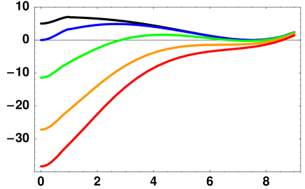
Figure 2: Thermal effective potential (27) for different values of the temperature. Going from bottom to top, the red line corresponds to the temperature $\Theta\gtrsim\Theta_{\rm crit}$ where we have only one vacuum at $\gamma=0$. The orange line corresponds to $\Theta\approx\Theta_{\rm crit}$ where the second vacuum appears and the classical rolling stops. The green line is in the interval $\Theta_{\rm degen}<\Theta<\Theta_{\rm crit}$ where one could hope to tunnel under the barrier. The blue line is at $\Theta\sim\Theta_{\rm degen}$ where the two vacua become degenerate. Finally, the black line gives the zero temperature potential where the non-supersymmetric vacuum at the origin becomes metastable.

In general one can consider a very wide range of temperatures $0\leq T\ll\Lambda_{L}$ corresponding to $0\leq\Theta\ll 1/(h\epsilon)$. From Fig. 2 where we have plotted the effective potential at various temperatures we immediately make out several interesting temperatures. At high enough temperature there is only one minimum at the origin and one would expect to be able to roll down classically to the non-supersymmetric minimum $|{\rm vac}\rangle_{+}$, as will be discussed in Section 3.2.3. Below $\Theta=\Theta_{\rm crit}$ a second minimum forms. It will turn out, that for our ISS potential this critical temperature will actually be less than $\gamma_{0}$. In the following analysis, we will consider the range of temperatures $h\mu<T\leq h\Phi_{0}$ corresponding to $1<\Theta\leq\gamma_{0}$.

At temperatures below $\Theta_{\rm crit}$ the SUSY breaking minimum at the origin still has lower free energy then $|{\rm vac}\rangle_{0}.$ We will calculate the bubble nucleation rate to the true vacuum $|{\rm vac}\rangle_{+}$ in Section 3.2.2. Another distinguished temperature $\Theta_{\rm degen}$ is when the SUSY preserving vacuum $|{\rm vac}\rangle_{0}$ becomes degenerate with the non-supersymmetric vacuum $|{\rm vac}\rangle_{+}$. For a generic potential one would expect that somewhere between these two scales there is a temperature $\Theta_{*}$ ($\Theta_{\rm degen}<\Theta_{*}\leq\Theta_{\rm crit}$) where the rate of bubble nucleation turns from large to small. Our main goal is to determine the temperature where the transitions (classical or tunnelling ones) from $|{\rm vac}\rangle_{0}$ to $|{\rm vac}\rangle_{+}$ stop.

3.2 Transition to a SUSY breaking vacuum and the lower bound on $\bm{T}_{R}$

In this subsection we discuss the two possibilities for the field to evolve to the SUSY breaking vacuum $|{\rm vac}\rangle_{+}$, classical evolution and bubble nucleation.

3.2.1 Classical evolution to the SUSY breaking vacuum: Estimate of $T_{\rm crit}$

It is clear from our expression for the thermal potential that at sufficiently high temperatures there is only one minimum, namely $|{\rm vac}\rangle_{+}$, and the SUSY preserving minimum disappears. This is caused by ${N_{f}}$ flavours of $\varphi$ and $\tilde{\varphi}$ becoming heavy away from the origin. The disappearance of $|{\rm vac}\rangle_{0}$ is most easily seen analytically in the limit of very high temperatures $\gamma\ll\Theta$ where the thermal potential grows as $\Theta^{2}\gamma^{2}$ in the $\gamma$ i.e. $\Phi$ direction,

$$\hat{V}_{\Theta}-\hat{V}_{\Theta=0}(\gamma)\sim\,N{N_{f}}\,\Theta^{2}\gamma^{2}-\,{\rm const}\,\Theta^{4}\ ,\qquad\Theta\gg\gamma=\Phi/\mu$$ (29)

Thus there is a critical temperature $\Theta_{\rm crit}$ such that at $\Theta>\Theta_{\rm crit}$ there is only one minimum, and at $\Theta<\Theta_{\rm crit}$ the supersymmetry preserving second minimum starts to materialise.

A better estimate can be obtained by using the approximation,

$$\pm\int_{0}^{\infty}\mbox{d}q\,q^{2}\ln\left(1\mp\exp(-\sqrt{q^{2}+\gamma^{2}/\Theta^{2}})\right)\sim\Theta^{4}\left(\frac{\gamma}{2\pi\Theta}\right)^{\frac{3}{2}}\exp\left(-\frac{\gamma}{\Theta}\right),\quad\rm{for}\quad\gamma\gg\Theta$$ (30)

for the integral in the $\Theta$ dependent part of Eq. (27). Comparing the derivatives (first and second) of the $\Theta$-dependent part and the $\Theta$-independent part of the effective potential $\hat{V}_{\Theta}$ in the vicinity of $\gamma_{0}$ we get an estimate,

$$\Theta_{\rm crit}\approx\,\frac{\gamma_{0}}{\log\left({\gamma^{4}_{0}}/{C}\right)}\ ,\qquad C=\,\frac{\sqrt{2}\pi^{\frac{3}{2}}}{Nh^{2}}\left(1-\frac{{N_{f}}}{N}\right)^{2}$$ (31)

which we have also confirmed numerically.

Although the height of the barrier in the zero temperature potential is only of the order of $\mu$ where $\mu\ll\gamma_{0}\mu=h\Phi_{0}$ the temperature necessary to erode the second minimum is only slightly (logarithmically) smaller than $h\Phi_{0}$ due to the exponential suppression $\sim\exp(-\gamma/\Theta)$ apparent in Eqs. (27) and (30).

In the early Universe the situation is not static and the temperature decreases due to the expansion of the Universe. So one should check that even in the absence of a second minimum the field has time enough to evolve to $|{\rm vac}\rangle_{+}$ before the temperature drops below $\Theta_{\rm crit}$. We will comment on this issue more in the next subsection. Here, we just point out that the temperature drops on a time scale $M_{Pl}/T^{2}\gg 1/T$.

3.2.2 Bubble Nucleation: Estimate of $T_{*}$

Let us now turn to the possibility of bubble nucleation, with an estimate of the temperature $T_{*}$ where the transitions from $|{\rm vac}\rangle_{0}$ to $|{\rm vac}\rangle_{+}$ change from fast to slow. Bubble nucleation is of course only possible above the temperature where the two minima become degenerate, so let us first estimate this. We compare the effective potential (27) at the origin

$$\hat{V}_{\Theta}(\gamma=0)=\,{(N-N_{f})}-\frac{\pi^{2}h^{2}\Theta^{4}}{90}\left(n_{B}+\frac{7}{8}n_{F}\right)$$ (32)

to the value of the effective potential at the second vacuum. The latter remains approximately zero since the temperature $T_{\rm degen}$ is much below $\Phi_{0}.$ In (32) $n_{B}(n_{F})$ counts the number of bosonic(fermionic) degrees of freedom ($4NN_{F}$ in both cases). We thus find

$$\Theta_{\rm degen}=\left({\frac{12(N_{f}-N)}{h^{2}\pi^{2}NN_{f}}}\right)^{\frac{1}{4}},\qquad\rm{for}\qquad\gamma_{0}\gg 1.$$ (33)

Now we would like to know when bubble nucleation is fast enough to lead to a phase transition. Thus we consider temperatures in the range $\Theta_{\rm degen}<\Theta<\Theta_{\rm crit}$ such that the second vacuum $|{\rm vac}\rangle_{0}$ is already formed but still higher than $|{\rm vac}\rangle_{+}$. In the following we want to estimate $\Theta_{*}$ where tunnelling becomes too slow.

For this purpose we will now derive a simple estimate on the action of the tunnelling trajectory in the thermal effective potential of the our model where the temperature is in the range $\Theta_{\rm degen}<\Theta\leq\Theta_{\rm crit}.$ The potential we want to model is depicted in Figure 2, its characteristic features are that the ‘false’ vacuum $|{\rm vac}\rangle_{0}$ is far away in the field space from $|{\rm vac}\rangle_{+}$ and that the potential climbs very slowly from $|{\rm vac}\rangle_{0}$ to a shallow barrier and then descends steeply to the ‘true’ vacuum $|{\rm vac}\rangle_{+}$. These features are a reflection of the fact that at zero temperature the vacuum $|{\rm vac}\rangle_{0}$ was generated non-perturbatively (as reviewed in the previous Section). We will model this class of potentials with a simple linear no-barrier potential,

$$\hat{V}_{\rm lin}(\gamma)=\,\theta(\eta-\gamma)\,{N_{f}}K\,(\gamma-\eta)$$ (34)

where $K$ and $\eta$ are constants, ${N_{f}}$ is put for convenience, and $\theta$ is the step-function. We plot this potential in Figure 2 for a convenient choice of constants along with the exact thermal potential. It is clear from this figure that the tunnelling rate for our model potential will always be a little higher than in the real case.

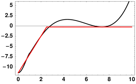
Figure 3: A simple no-barrier model for the thermal effective potential. The modelling potential $\hat{V}_{\rm lin}(\gamma)$ is shown in red and the exact thermal potential $\hat{V}_{T}(\gamma)$is black. The tunnelling rate to the true vacuum for this model is calculated in the text.

The potential (34) admits a simple analytic solution for the bounce configuration. The tunnelling in this potential was discussed in detail in Ref. [26] in the $T=0$ case. We have performed a similar calculation in the 3-dimensional settings relevant to the thermal case. The tunnelling configuration is the bounce solution $\gamma_{\rm bounce}(x)$ which extremizes the 3-dimensional action

$$\frac{1}{T}\,S^{3D}=\,\frac{1}{T}\,4\pi\int dr\,r^{2}\left({\textstyle{1\over 2}}{\rm Tr}_{{N_{f}}}(\Phi^{\prime})^{2}+V_{T}(\Phi)\right)=\,{N_{f}}\,\frac{4\pi}{\Theta h^{2}}\,\int dx\,x^{2}\left({\textstyle{1\over 2}}(\gamma^{\prime})^{2}+\frac{1}{{N_{f}}}\,\hat{V}_{\rm lin}(\gamma)\right)$$ (35)

with the appropriate initial conditions. The right hand side of (35) is written in terms of our usual dimensionless variables $\gamma,$ $\Theta$ and the rescaled radial distance $x=h\mu r$. The classical equation for the bounce is then

$$\gamma^{\prime\prime}+\frac{2}{x}\gamma^{\prime}=\,{\frac{1}{{N_{f}}}}\,\partial_{\gamma}\hat{V}(\gamma)$$ (36)

For the case (34) the bounce solution reads

$$\gamma_{\rm bounce}(x) = \left\{\begin{array}[]{cc}\frac{1}{6}Kx^{2}&\qquad x\leq x_{m}\\ 3\eta-2\eta\frac{x_{m}}{x}&\qquad x\geq x_{m}\end{array}\right.$$ (39)

where $x_{m}=\sqrt{\frac{6\eta}{K}}$ is the matching point for the two branches of the bounce solution and of its derivative. The field configuration (39) describes a bubble of size $x_{m}$ with $\gamma=3\eta$ on the outside at large $x\gg x_{m},$ and $\gamma=0$ on the inside at $x=0.$ The asymptotic value of $\gamma_{\rm bounce}$ is the ‘false’ vacuum $|{\rm vac}\rangle_{0}$, thus we should identify $3\eta$ with $\gamma_{0}.$

The action (35) on the bounce trajectory is

$$\frac{1}{T}\,S^{3D}_{\rm bounce}=\,\frac{4\pi}{\Theta h^{2}}\,{N_{f}}\,\frac{8\sqrt{6}}{5}\,\frac{\eta^{2+\frac{1}{2}}}{K^{\frac{1}{2}}}$$ (40)

Now using the identification $3\eta=\gamma_{0}$ and ${N_{f}}K\eta\propto\Delta\hat{V},$ where $\Delta\hat{V}$ is the drop in the potential which should be taken to be $\Delta\hat{V}\propto\Theta^{4}$ we get

$$\frac{1}{T}\,S^{3D}_{\rm bounce}\,\approx{\rm const}\,\left(\frac{\Phi_{0}}{T}\right)^{3}$$ (41)

using the original dimensional variables $\Phi_{0}$ and $T$. In order for the Universe to have undergone a phase transition by bubble nucleation one requires a sufficiently high nucleation probability of bubbles of metastable vacuum. The nucleation rate is given by

$$\Gamma_{3}\sim T^{4}e^{-S^{3D}/T}.$$ (42)

This rate must be integrated from a maximum (reheat) temperature $T_{R}$ to the temperature $T_{\rm degen}\sim\mu$ at which the metastable and supersymmetric minima are degenerate. The fraction of space remaining in the broken phase is $e^{-P}$ where [19]

$$P \sim \frac{M_{Pl}^{4}}{T_{0}^{3}}\int_{T_{\rm degen}}^{T_{R}}\,T^{-2}(1-T_{0}/T)^{3}e^{-S^{3D}/T}dT$$ (43)

$$\approx \frac{M_{Pl}^{4}}{3T_{0}^{3}S^{3D}}\,e^{-\frac{S^{3D}}{T_{R}}}$$ (44)

where $T_{0}$ is the temperature of the Universe today. This gives

$$P\sim e^{256-\frac{S^{3D}}{T_{R}}}\,\frac{M_{W}}{S^{3D}}$$ (45)

and the bound becomes $\frac{\Phi_{0}}{T_{R}}\lesssim 1.3$. From this we conclude that the temperature $T_{*}$ at which the tunnelling transitions are still possible is very high (at the very top of its defining range),

$$T_{*}\,\gtrsim\,\Phi_{0}\ ,\qquad{\rm or}\qquad\Theta_{*}\,\gtrsim\gamma_{0}$$ (46)

The temperature where bubble nucleation becomes significant has the same parametric dependence as the critical temperature $\Theta_{\rm crit}$ (our simple estimate is insufficient to capture logarithmic dependencies) and we conclude that $T_{*}\sim T_{\rm crit}$.

3.2.3 Behaviour of the field after nucleation/rolling

If the temperature rises above the critical temperature, the field is in principle free to roll; however, is the critical temperature a sufficient condition for the field to always end up at the origin? Assuming that the Universe evolves in the standard FRW manner, we should check that the phase transition has time to complete, and that the falling temperature does not “overtake” the field. In order to model the field after the transition, we can approximate the potential at temperatures above $T_{\rm crit}$ as linear;

$$V=\,{\rm const}\,T^{4}\,\frac{\Phi}{\Phi_{0}}-{\rm const^{\prime}}$$ (47)

Neglecting for the moment the effect of the $\varphi\Phi\tilde{\varphi}$ coupling, the field equations are

$$\ddot{\Phi}+3H\dot{\Phi}=\,-{\rm const}\,\frac{T^{4}}{\Phi_{0}}.$$ (48)

We may assume that the Hubble constant $H\sim T^{2}/M_{Pl}$ is negligible in this equation, so, taking initial values $T_{0}\gtrsim T_{\rm crit}$ i.e. $T_{0}\sim\Phi_{0}$, we find that the field falls to the origin in time

$$\Delta t_{\rm roll}\sim\,\frac{\Phi_{0}}{T_{0}^{2}}\sim\,\frac{1}{T_{0}}\sim\,M_{Pl}^{-\frac{1}{2}}t_{0}^{\frac{1}{2}}$$ (49)

where on the right hand side $t_{0}$ defines the time at which the temperature is $T_{0},$ and we have considered a radiation dominated Universe with scale factor $a(t)\sim(t/t_{0})^{\textstyle{1\over 2}}.$ The result (49) should be compared to the typical time necessary for the Universe to cool to temperatures where the second minimum $|{\rm vac}\rangle_{0}$ becomes prominent. The evolution of $T$ is given by

$$T(t)=\,\frac{T_{0}}{a(t)}\sim\,T_{0}\,\left(\frac{t_{0}}{t}\right)^{\textstyle{1\over 2}}$$ (50)

For example the time needed to reach $T=T_{0}/\sqrt{2}$ is $\Delta t_{\rm cool}=t_{0}$ which gives $\Delta t_{\rm cool}\gg\Delta t_{\rm roll}.$ This means that the field is able to roll essentially instantaneously to the origin where it undergoes coherent oscillation.

Having concluded that the fields roll down to $|{\rm vac}\rangle_{+}$ sufficiently fast, we still need to check that the oscillations of the fields around $|{\rm vac}\rangle_{+}$ would not bring us back to $|{\rm vac}\rangle_{0}$ as the Universe cools. It is easy to see that if there was only the Hubble damping the $\Phi$ field would oscillate out of the origin as the Universe cools. Indeed, the $\Phi$ oscillations essentially preserve energy in a comoving volume;

$$m_{\Phi}^{2}\Phi_{\rm max}^{2}R^{3}=\mbox{const~{},}$$ (51)

where $R\sim t^{\frac{1}{2}}$ is the scale factor in a radiation dominated Universe, and $m_{\Phi}=\frac{hT}{2}$ is the temperature induced mass of $\Phi$ at the origin. In an adiabatic regime $RT=const$ so we find

$$\frac{\Phi_{\rm max}(T)}{\Phi_{0}} = \sqrt{\frac{T}{T_{0}}}.$$ (52)

The field would then escape from the origin because when $T\sim\mu$, (assuming $T_{0}\sim\Phi_{0}$) the size of the oscillations would be

$$\Phi_{\rm max}\sim\sqrt{\Phi_{0}\mu}\gg\mu.$$ (53)

Fortunately, any open decay channel of $\Phi$ will typically provide a damping rate $\Gamma_{\Phi}\sim T$, capturing the field in $|{\rm vac}\rangle_{+}$. An example are couplings to the messenger sector fields, $f$, of the form $h^{\prime}\tilde{f}\Phi f.$ Since we assume thermal equilibrium, such a coupling must exist and cannot be arbitrarily weak. The decaying oscillation amplitudes are of order

$$\frac{\Phi_{\rm max}(T)}{\Phi_{0}} = \sqrt{\frac{T}{T_{0}}}e^{-\frac{1}{2}\Gamma_{\Phi}(t-t_{0})}.$$ (54)

Sufficient damping always occurs; imposing $\Phi_{\rm max}<\mu$ requires only that $\frac{M_{Pl}}{\Phi_{0}}\stackrel{{\scriptstyle>}}{{\sim}}\log(\Phi_{0}/\mu)$ which is always satisfied and the Universe ends up in the SUSY breaking state $|{\rm vac}\rangle_{+}.$ Note, however, that the number of oscillations before damping is proportional to $\log(\Phi_{0}/\mu$) and may be large.

3.2.4 Lower bound on reheating temperature $T_{R}$

Now, let us summarize our analysis and explain under which conditions it is natural for the early Universe to settle down at the metastable SUSY breaking vacuum. At the end of inflation the Universe is in a state of very low temperature and one may assume that it is in the energetically preferred supersymmetric state $|{\rm vac}\rangle_{0}$. After inflation the Universe reheats to a temperature $T_{R}$. Already at relatively low temperatures $\sim T_{\rm degen}\sim\mu$ the supersymmetry breaking vacuum will have lower free energy than the supersymmetric vacuum. However, if $T_{R}$ falls in the range $T_{\rm degen}<T_{R}\lesssim T_{*}\sim T_{\rm crit}$, the Universe will remain in the state $|{\rm vac}\rangle_{0}$ although $|{\rm vac}\rangle_{+}$ is energetically preferred. It is stuck there because the barrier makes classical evolution impossible and bubble nucleation is too slow. Above $T_{*}$ the bubble nucleation rate will be high and above $T_{\rm crit}$ the classical evolution becomes possible. Hence, the Universe will evolve to the preferred supersymmetry breaking state $|{\rm vac}\rangle_{+}$. We conclude that if the reheating temperature $T_{R}$ fulfills

$$T_{\rm crit}\sim\frac{\mu}{\epsilon^{1-2N/(N_{f}-N)}}\,\lesssim\,T_{R}\,\lesssim\,\frac{\mu}{\epsilon}$$ (55)

it is ensured that the Universe always ends up in the supersymmetry breaking ground state $|{\rm vac}\rangle_{+}.$

In principle one should also consider the possibility of a transition back towards the SUSY vacuum for $T<T_{\rm{degen}}$. It is known that this does not happen at zero temperature [1] . We have made a simple estimate of this effect at $T>0$ and concluded that the Universe remains trapped. More recently, this has been discussed in depth in [15, 16, 17].

The condition (23) or (24) that the metastable vacuum $|{\rm vac}\rangle_{+}$ is long-lived at zero temperature does not necessarily require $\Phi_{0}$ to be very large or $\epsilon^{1-2N/(N_{f}-N)}$ to be very small. For a low supersymmetry breaking scale $\mu$ of order of a few TeV the lower bound on the reheating temperature in (55) can be easily satisfied for reheating temperatures as low as around 10 or 100 TeV. On the other hand, for models with a significantly higher SUSY breaking scale, this bound becomes more constraining.

4 Conclusions and discussion

We have examined the consequences of meta-stable SUSY breaking vacua in a cosmological setting. As noted in [1], the ISS theory naturally admits a finite number of isolated supersymmetric vacua (as determined by the Witten index) along with a larger moduli space of metastable SUSY breaking vacua. Since the latter is a much bigger configuration space, ISS suggested that it is more favorable for the Universe to be populated in the metastable SUSY breaking vacua. In this paper, we have considered thermal effects in the ISS model and have shown that the early Universe is always driven to metastability: as long as the SUSY breaking sector is in thermal equilibrium this provides a generic, dynamical explanation why supersymmetry became broken. This phenomenon is a consequence of two distinguishing properties of the ISS theory which are not necessarily shared by other models with metastable SUSY breaking vacua, namely, that the metastable minima have more light degrees of freedom than the SUSY preserving vacua, and that the metastable vacua are separated from the SUSY preserving vacuum by a very shallow dynamically induced potential. Both play significant roles in our argument and our various estimates.

Given the current interest in ”landscapes” of one variety or another, it is difficult to resist speculating on their implications for the ISS models, given the conclusions of our study. One longstanding problem that can be addressed in this context is that of the hierarchy between the Planck and supersymmetry breaking scales. Consider the possibility that the SUSY breaking sector has in fact a large number of product groups, with a landscape of metastable ISS minima into which the Universe could be thermally driven, with a range of values of SUSY breaking. The very existence of the lower bound on $T_{R}$ implies that there is a maximal value of a SUSY breaking scale $\mu$ which characterizes metastable vacua we can reach as the Universe cools down. Using our estimate for $T_{R},$ Eq. (55) we find

$$\mu\sim\Lambda_{L}\left(\frac{T_{R}}{\Lambda_{L}}\right)^{\frac{N_{f}-N}{2N}},$$ (56)

where $\Lambda_{L}$ is the Landau pole of the theory. Thus not only is the SUSY breaking determined to lie below $\Lambda_{L}$, it is also parametrically suppressed by powers of $T_{R}/\Lambda_{L}$.

References

- [1] K. Intriligator, N. Seiberg and D. Shih, “Dynamical SUSY breaking in meta-stable vacua,” JHEP 0604 (2006) 021 hep-th/0602239.
- [2] J. R. Ellis, C. H. Llewellyn Smith and G. G. Ross, “Will The Universe Become Supersymmetric?,” Phys. Lett. B 114 (1982) 227.
- [3] S. Franco and A. M. Uranga, “Dynamical SUSY breaking at meta-stable minima from D-branes at obstructed geometries,” JHEP 0606 (2006) 031 hep-th/0604136.
-
[4]
H. Ooguri and Y. Ookouchi,
“Landscape of supersymmetry breaking vacua in geometrically realized gauge theories,”
hep-th/0606061;
“Meta-stable supersymmetry breaking vacua on intersecting branes,” Phys. Lett. B 641 (2006) 323 hep-th/0607183. -
[5]
V. Braun, E. I. Buchbinder and B. A. Ovrut,
“Dynamical SUSY breaking in heterotic M-theory,”
Phys. Lett. B 639 (2006) 566
hep-th/0606166;
“Towards realizing dynamical SUSY breaking in heterotic model building,” JHEP 0610 (2006) 041 hep-th/0606241. - [6] R. Argurio, M. Bertolini, S. Franco and S. Kachru, “Gauge / gravity duality and meta-stable dynamical supersymmetry breaking,” hep-th/0610212.
- [7] S. Franco, I. Garcia-Etxebarria and A. M. Uranga, “Non-supersymmetric meta-stable vacua from brane configurations,” hep-th/0607218.
- [8] S. Forste, “Gauging flavour in meta-stable SUSY breaking models,” hep-th/0608036.
- [9] A. Amariti, L. Girardello and A. Mariotti, “Non-supersymmetric meta-stable vacua in SU(N) SQCD with adjoint matter,” hep-th/0608063.
- [10] I. Bena, E. Gorbatov, S. Hellerman, N. Seiberg and D. Shih, “A note on (meta)stable brane configurations in MQCD,” hep-th/0608157.
- [11] M. Dine, J. L. Feng and E. Silverstein, “Retrofitting O’Raifeartaigh models with dynamical scales,” hep-th/0608159.
- [12] C. Ahn, “Brane configurations for nonsupersymmetric meta-stable vacua in SQCD with adjoint matter,” hep-th/0608160; “M-theory lift of meta-stable brane configuration in symplectic and orthogonal gauge groups,” hep-th/0610025.
- [13] M. Eto, K. Hashimoto and S. Terashima, “Solitons in supersymmety breaking meta-stable vacua,” hep-th/0610042.
- [14] M. Aganagic, C. Beem, J. Seo and C. Vafa, “Geometrically induced metastability and holography,” hep-th/0610249.
- [15] N. J. Craig, P. J. Fox and J. G. Wacker, “Reheating metastable O’Raifeartaigh models,” hep-th/0611006.
- [16] W. Fischler, V. Kaplunovsky, C. Krishnan, L. Mannelli and M. Torres, “Meta-stable supersymmetry breaking in a cooling universe,” hep-th/0611018.
- [17] S. A. Abel, J. Jaeckel and V. V. Khoze, “Why the early universe preferred the non-supersymmetric vacuum. II,” JHEP 0701 (2007) 015 hep-th/0611130.
-
[18]
G. W. Anderson, A. D. Linde and A. Riotto,
“Preheating, supersymmetry breaking and baryogenesis,”
Phys. Rev. Lett. 77 (1996) 3716
hep-ph/9606416;
A. Riotto, E. Roulet and I. Vilja, “Preheating and vacuum metastability in supersymmetry,” Phys. Lett. B 390 (1997) 73 hep-ph/9607403. -
[19]
A. Riotto and E. Roulet,
“Vacuum decay along supersymmetric flat directions,”
Phys. Lett. B 377 (1996) 60
hep-ph/9512401;
A. Strumia, “Charge and color breaking minima and constraints on the MSSM parameters,” Nucl. Phys. B 482 (1996) 24 hep-ph/9604417;
T. Falk, K. A. Olive, L. Roszkowski, A. Singh and M. Srednicki, “Constraints from inflation and reheating on superpartner masses,” Phys. Lett. B 396 (1997) 50 hep-ph/9611325;
S. A. Abel and C. A. Savoy, “On metastability in supersymmetric models,” Nucl. Phys. B 532 (1998) 3 hep-ph/9803218;
“Charge and colour breaking constraints in the MSSM with non-universal SUSY breaking,” Phys. Lett. B 444 (1998) 119 hep-ph/9809498. - [20] N. Seiberg, “Exact Results On The Space Of Vacua Of Four-Dimensional SUSY Gauge Theories,” Phys. Rev. D 49 (1994) 6857 hep-th/9402044.
- [21] N. Seiberg, “Electric - magnetic duality in supersymmetric non-Abelian gauge theories,” Nucl. Phys. B 435 (1995) 129 hep-th/9411149.
- [22] K. A. Intriligator and N. Seiberg, “Lectures on supersymmetric gauge theories and electric-magnetic duality,” Nucl. Phys. Proc. Suppl. 45BC (1996) 1 hep-th/9509066.
-
[23]
R. A. Flores and M. Sher,
“Upper Limits To Fermion Masses In The Glashow-Weinberg-Salam Model,”
Phys. Rev. D 27 (1983) 1679;
M. J. Duncan, R. Philippe and M. Sher, “Theoretical Ceiling On Quark Masses In The Standard Model,” Phys. Lett. B 153 (1985) 165 [Erratum-ibid. 209B (1988) 543];
P. B. Arnold, “Can The Electroweak Vacuum Be Unstable?,” Phys. Rev. D 40 (1989) 613;
G. W. Anderson, “New cosmological constraints on the higgs boson and top quark masses,” Phys. Lett. B 243 (1990) 265;
P. Arnold and S. Vokos, “Instability of hot electroweak theory: bounds on m(H) and M(t),” Phys. Rev. D 44 (1991) 3620;
J. R. Espinosa and M. Quiros, “Improved Metastability Bounds On The Standard Model Higgs Mass,” Phys. Lett. B 353 (1995) 257 hep-ph/9504241. - [24] L. Dolan and R. Jackiw, “Symmetry Behavior At Finite Temperature,” Phys. Rev. D 9, 3320 (1974).
- [25] T. Falk, K. A. Olive, L. Roszkowski and M. Srednicki, “New Constraints on Superpartner Masses,” Phys. Lett. B 367 (1996) 183 hep-ph/9510308.
- [26] K. M. Lee and E. J. Weinberg, “Tunneling Without Barriers,” Nucl. Phys. B 267, 181 (1986).