Open strings in Lie groups and associative products

Abstract

Firstly, we generalize a semi-classical limit of open strings on D-branes in group manifolds. The limit gives rise to rigid open strings, whose dynamics can efficiently be described in terms of a matrix algebra. Alternatively, the dynamics is coded in group theory coefficients whose properties are translated in a diagrammatical language. In the case of compact groups, it is a simplified version of rational boundary conformal field theories, while for non-compact groups, the construction gives rise to new associative products. Secondly, we argue that the intuitive formalism that we provide for the semi-classical limit, extends to the case of quantum groups. The associative product we construct in this way is directly related to the boundary vertex operator algebra of open strings on symmetry preserving branes in WZW models, and generalizations thereof, e.g. to non-compact groups. We treat the groups $SU(2)$ and $SL(2,\mathbb{R})$ explicitly. We also discuss the precise relation of the semi-classical open string dynamics to Berezin quantization and to star product theory.

1 Introduction

Theories of quantum gravity are expected to be non-local. String theory, a prominent theory of quantum gravity, is indeed non-local. A non-commutative subsector of string theory has been identified that decouples from gravity, but that retains some of the non-locality of string theory. (See e.g. [1] and references therein, and [2] for a review.) That discovery gave rise to the further study of non-commutative field theories [3], and the associated mathematical structures. One can be hopeful that the study of these theories will teach us more about how to sensibly formulate non-local theories of quantum physics and non-local theories of quantum gravity.

In this article, we study a class of non-commutative theories. Our study is motivated by the physics of open strings on D-branes in group manifolds, but will not be restricted to this setting only, and it will be explained in elementary and general terms. For open strings on group manifolds, the above limit, decoupling from gravity, but keeping highly non-trivial (non-commutative) gauge theory dynamics is also available. It gives rise to the study of non-commutative gauge theories on curved manifolds (see e.g. [4]).

In particular, we will firstly concentrate on a semi-classical limit of open strings on generic group manifolds. This will have the advantage of considerably simplifying the analysis of the open string dynamics (while sacrifying finite bulk curvature effects). This will allow us to provide an elegant semi-classical picture of open string dynamics on group manifolds. In order to present it, and to show its generality, we delve into the theory of quantization of co-adjoint orbits (which describes the behavior of one end of an open string), the quantization of pairs of orbits (for the two endpoints of an open string) and the composition of operators on the resulting Hilbert spaces (corresponding to the concatenation of open strings).

For compact Lie groups, this part of our analysis is a simpler, limiting version of the analysis of chiral classical conformal field theory [5], or boundary vertex operator algebras [6]. We believe that providing an intuitive and precise picture for the semi-classical limit of rational boundary conformal field theory is interesting in its own right, and we furthermore show that the picture also applies to non-rational boundary conformal field theory which is much less understood. Thus, we are able to put our construction to good use, by explicitly applying it to the example of non-compact groups. Moreover, it will enable us to provide a proposal for a mathematical program quantizing symplectic leaves of Poisson manifolds, and providing a product of operators associated to triples of symplectic leaves.

Secondly, we argue that our intuitive picture that holds for quantization for orbits of Lie groups, can be extended to quantum groups, and that in doing so, we can recuperate the full solution to rational boundary conformal field theories in the case of symmetry preserving D-branes in Wess-Zumino-Witten models on compact groups, and that the construction will generalize to non-compact groups.

Since we make reference to a lot of concepts that have been highly developed by different communities, we are not able to review them all fully. Our strategy will be to first illustrate the concepts in the simple case of the group $SU(2)$. We then sketch how to obtain much more general results on these structures by citing the relevant references. In this way, we hope to show generality while preserving intuition. We follow this strategy in section 2 that reviews the orbit method, in section 3 that generalizes it to pairs of orbits, in section 5 that reviews the structure constants for the $SU(2)$ case, as well as in appendix B where we review some facts concerning Berezin quantization and star product theory. Section 3 introduces and analyzes the action for rigid open strings on group manifolds, and in sections 6 and 7 we work out how our formalism applies to the non-compact group $SL(2,\mathbb{R})$. Finally, we treat the case of quantum groups in section 8.

2 Co-adjoint orbit quantization

We start building an elementary picture of open string interactions by concentrating on one of the endpoints of the open string (see figure 1).

Figure 1: We concentrate first on one endpoint of an open string.

Using the mathematical framework of the orbit method, we quantize the associated degrees of freedom .

2.1 An electric charge in the presence of a magnetic monopole

In this subsection, we analyze the quantization of a charged particle on a sphere, with a magnetic monopole sitting at the center of the sphere. The particle will only interact electromagnetically. We show that the quantization of the particle boils down to the quantization of a co-adjoint orbit of $SU(2)$.

The magnetic monopole

We consider the three-dimensional flat space $\mathbb{R}^{3}$, with spherical coordinates:

$$x^{1} = r\sin\theta\cos\phi$$

$$x^{2} = r\sin\theta\sin\phi$$

$$x^{3} = r\cos\theta$$ (1)

We put a magnetic monopole of integer charge $n$ at the origin of the coordinate system $x^{i}=0$. We can describe the magnetic field it generates in terms of the vector potentials:

$$A^{\pm} = \frac{n}{2}(\pm 1-\cos\theta)d\phi$$

$$F = dA^{\pm}=\frac{n}{2}\sin\theta d\theta\wedge d\phi$$

$$A^{+} = A^{-}+nd\phi=A^{-}+d(n\phi)$$ (2)

where the vector potentials are valid near north ($\theta=0$) and south ($\theta=\pi$) poles respectively (since we avoid a conical singularity there due to the $\pm 1$ in the potential), and where the relation between the two potentials is a gauge transformation on the overlap, which is well-defined provided $n$ is indeed integer.

A charged particle on the sphere

Next, we introduce a charged particle, and we constrain it on a sphere in the presence of the magnetic monopole (see figure 2).

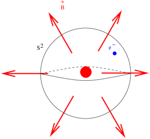
Figure 2: An electron bound to a sphere, with a magnetic monopole in the middle of the sphere.

As an action, we take the electromagnetic coupling only [7, 8]:

$$S=\int A^{\pm}=\frac{n}{2}\int d\tau(\pm 1-\cos\theta)\dot{\phi}$$ (3)

The equations of motion are easily derived, and they imply that the velocity of the particle is zero. The solutions to the equations of motion thus correspond to the particle sitting at a fixed point of the two-sphere. Thus, the classical phase space, which is the space of classical solutions, is the two-sphere.

The global symmetries of the problem at hand are the $SU(2)$ rotations which act transitively on the phase space. The charges associated to the $SU(2)$ global symmetries are the positions $x^{i}$ of the particle, which are indeed conserved (since the particle does not move). They can be shown to satisfy $SU(2)$ commutation relations under the Dirac bracket (see e.g. [9]). The Hamiltonian of the purely topological action $(\ref{san})$ is zero.

2.2 A classical particle on a co-adjoint orbit

To generalize the well-known facts discussed above, we observe that the gauge potential can be viewed as arising from the following general formula for a one-form defined on a group manifold:

$$\theta_{\lambda}(g) = \langle\lambda,g^{-1}dg\rangle$$ (4)

where $g$ is a group element of a Lie group $G$, $\lambda$ is an element of the dual of the Lie algebra ${\cal G}^{\ast}$ and the bracket $\langle.,.\rangle$ denotes the evaluation of $\lambda$ on the element of the Lie algebra $g^{-1}dg$. Now that we have defined the one-form, we can pull it back onto the world-line $L$ of a particle via the map of the particle into the group manifold $g:L\mapsto G:\tau\mapsto g(\tau)$, and we can define the action of the particle as the integral over the world-line of this one-form. It is an easy calculation to show that this action for the case of $SU(2)$ precisely coincides with the action introduced above [8]. However, we can now generalize this action to any group manifold, once we are given an element $\lambda$ of the dual Lie algebra [8]:

$$S = \int_{L}d\tau<\lambda,g^{-1}\partial_{\tau}g>$$ (5)

Again, the Hamiltonian corresponding to the action is zero. It is interesting to analyze the symmetries of this action. The global symmetry is $G$ which acts on the particle trajectory $g$ by multiplication on the left. The local symmetry, i.e. the gauge group, is the stabilizer of the weight $\lambda$, and it acts by multiplication on the right. The local symmetry makes for the fact that the particle is interpreted not as moving on the full group manifold $G$, but rather on the manifold $G/Stab(\lambda)$ (which for the case of $SU(2)$ is the two-sphere $SU(2)/U(1)=S^{2}$), which coincides with the phase space.

The conserved Noether charges associated to the global symmetry group are $I=g\lambda g^{-1}$ and they satisfy the Dirac brackets with the structure constants equal to the structure constants of the Lie algebra of the group [9]. (They are the generalization of the positions $x^{i}$.) The symmetry group $G$ acts transitively on the phase space. The global charges and functions thereof are gauge invariant observables of the theory.

2.3 The quantization

In this subsection, we quantize the classical theory, starting out with the $SU(2)$ example before generalizing to other groups.

The quantization of the spherical phase space

We can quantize the phase space to find the Hilbert space. The dimension of the Hilbert space is the number of Planck cells that fit into the two-sphere. The symplectic form arising from the action is the volume form of the two-sphere with quantized overall coefficient, and consequently (after a straightforward calculation) the number of Planck cells in phase space is computed to be the integer number $n$. Since the group $SU(2)$ is represented on the Hilbert space, we find a spin $j=\frac{n-1}{2}$ representation of $SU(2)$ as the Hilbert space of the particle. The group acts transitively on the classical phase space, and is represented irreducibly on the quantum Hilbert space.

We note that the (closed) Wilson loop $\exp(\imath\int A)$ (which in the quantum theory weighs the path integral) and the quantization of the coefficient of the action (which is the magnetic monopole charge) can also be obtained by demanding that the path integral be well-defined for closed world-line trajectories. Namely, the action should not be ambiguous, up to a multiple of $2\pi\imath$. Since the action can be computed by calculating the flux either through the cap or the bowl (i.e. filling in the Wilson loop (see figure 3) either over the north or the south pole), we must have that the difference (divided by $2\pi\imath$) is quantized.

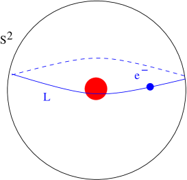
Figure 3: The (blue) curve traced by the electron associated to a Wilson loop. The Wilson loop can be computed by calculating the flux through the upper cap (– the hat –) or the lower cap (– the bowl –), and must be unambiguous.

Thus, the (half-integer) quantization of spin $j$ in this context is re-interpreted in the electron/magnetic monopole system as being associated to the Dirac quantization condition for the product of electric and magnetic charge $n$. Also, invariance of the action up to a multiple of $2\pi\imath$ (which is the condition of well-definedness of the quantum path integral), corresponds in the geometric language to the fact that the two-sphere needs to be integral [10]. Alternatively, in geometric quantization, the $U(1)$ bundle over the two-sphere needs to be well-defined. All these features are explained in terms of physics and fiber bundles in [9] where the above constrained system is also canonically quantized. The path integral approach to quantization was developed in references [7, 8]. Different regularizations of the path integral exist (see e.g. [8] and the appendix of [11]) which can also be understood as different types of geometric quantization (namely naive, or metaplectic geometric quantization in the nomenclature of [12]). These different regularizations give slight shifts in the interpretation of the coefficient of the action (as twice the spin or rather $2j+1$). (In the mathematics literature as well (see e.g. [10]) this ambiguity is well-known.)

2.4 The orbit method

We very briefly review the highly developed domain of co-adjoint orbit quantization. See e.g. [10] for a summary.

The orbit method constructs the irreducible representations of a Lie group $G$ via the study of its co-adjoint orbits. A co-adjoint orbit $O_{\lambda}$ can be defined as the set obtained from a fixed representative $\lambda$, an element of the dual of the Lie algebra of the group, by the co-adjoint action of the group (i.e. by conjugation with a group element). A co-adjoint orbit has a canonical symplectic form $\omega_{\lambda}$, which can locally be described as the derivative of the one-form $\theta_{\lambda}$ we introduced above:

$$\omega_{\lambda} = d\theta_{\lambda}$$ (6)

To quantize the orbit, we need the integral of the symplectic form over closed two-cycles to be an integer – this is the generalization of the Dirac quantization condition. Orbits satisfying this condition are called integral orbits. The orbits can then be quantized (see figure 4)

Figure 4: The quantized orbit $O_{\lambda}$, on which the open string endpoint lives, is divided into phase space cells of size $h$ where $h$ is Planck’s constant.

and each orbit gives rise to a Hilbert space which is an irreducible representation of the group $G$.

A point we wish to stress here is that this construction is very generic. When applied to $SU(2)$ it gives the results above, and when applied to compact groups, one recuperates all irreducible representations of the compact group, via the Borel-Weyl-Bott theorem (see e.g. [10]). But we note that the orbit method has been successfully applied to a much larger class of groups, including nilpotent groups, exponential groups, solvable groups in general, as well as other finite dimensional non-compact groups. Moreover, it has been successfully applied to infinite dimensional groups as well, like the Virasoro group and loop groups. We refer to [10] for an extended list of references and also to [13] for many references within the physics literature.

3 Pairs of orbits

In this section, we discuss the addition of a second charged particle to our physical problem. It corresponds to the second endpoint of the open string (see figure 1). Firstly, we discuss briefly the case where the two endpoints do not interact, and then we discuss an interaction term which coincides with the Hamiltonian for rigid open strings.

Tensoring for two

We add a second particle and define in a first step its action to be again the purely electromagnetic coupling, but with the opposite sign for the charge (or equivalently, the opposite sign symplectic form). We can add this particle to the same orbit as the first particle, but we can also choose to constrain it to its own orbit. After quantization, we find that the combined two-particle system has a Hilbert space which is the tensor product of the $\lambda_{I}$ representation of the first particle and the $\bar{\lambda_{F}}$ representation of the second particle. (The indices $I,F$ indicate the initial and the final endpoints of the string, respectively. The bar on $\lambda_{F}$ reminds us that we quantize with the opposite sign symplectic form, giving rise to the conjugate representation.)

The action for the uncoupled system is simply the sum of the two individual particle actions:

$$S_{2-particle} = \int_{L}d\tau<\lambda_{I},g^{-1}_{I}\partial_{\tau}g_{I}>-\int_{L}d\tau<\lambda_{F},g^{-1}_{F}\partial_{\tau}g_{F}>$$ (7)

The global symmetry is doubled to $G_{I}\times G_{F}$, the local symmetry group becomes $Stab(\lambda_{I})\times Stab(\lambda_{F})$, and we perform a path integral over both particle trajectories $g_{I}$ and $g_{F}$. The conserved charges and equations of motion are easily determined as in the previous section. Let’s now introduce an interaction term.

The rigid string tension

Although we have been arguing continuously with the intuitive image of an open string in the back of our minds, we have not yet demonstrated the precise connection between our construction and the physics of open strings. We will make the connection precise in this subsection. The rigid string we construct will correspond to two charged particles connected by a spring. To represent the spring, we add a potential term to the action that is proportional to the distance squared between the two endpoints of the string. We suppose that a non-degenerate bi-invariant metric on the Lie algebra exists, and we measure the distance between the end-points in this metric. The metric allows us to identify the Lie algebra with its dual. The bracket operation $\langle.,.\rangle$ then represents evaluation of the norm in the invariant metric. The action is:

$$S = \int_{L}d\tau\left(<\lambda_{I},g_{I}^{-1}\partial_{\tau}g_{I}>-<\lambda_{F},g_{F}^{-1}\partial_{\tau}g_{F}>\right)$$ (8)

$$+\frac{K}{2}\int_{L}d\tau<g_{I}\lambda_{I}g_{I}^{-1}-g_{F}\lambda_{F}g_{F}^{-1},g_{I}\lambda_{I}g_{I}^{-1}-g_{F}\lambda_{F}g_{F}^{-1}>$$

Firstly, we notice that $g_{I,F}$ can still be separately gauge transformed, and they live in the manifold $G/Stab(\lambda_{I,F})$, respectively. The global symmetry group is broken however, by the interaction term, to a diagonal left action on both group elements.

The classical dynamics of the system is solved for as follows. The equations of motion are:

$$\partial_{\tau}(g_{I}\lambda_{I}g_{I}^{-1})+K{[}g_{I}\lambda_{I}g_{I}^{-1},g_{F}\lambda_{F}g_{F}^{-1}{]} = 0$$

$$-\partial_{\tau}(g_{F}\lambda_{F}g_{F}^{-1})+K{[}g_{F}\lambda_{F}g_{F}^{-1},g_{I}\lambda_{I}g_{I}^{-1}{]} = 0$$ (9)

where ${[},{]}$ denotes the commutator. We can read off from these equations the conserved currents associated to the global symmetry. We define the (non-conserved) charges $I_{I}=g_{I}\lambda_{I}g_{I}^{-1}$ and $I_{F}=-g_{F}\lambda_{F}g_{F}^{-1}$ which generate the same algebra (because of the opposite sign of the charges and of the symplectic structures for the final point compared to the initial point). Note that the second charge $I_{F}$ corresponds to minus the position of the final end-point of the string. The sum of these charges is conserved:

$$\partial_{\tau}(I_{I}+I_{F}) = 0$$ (10)

It generates the simultaneous translation $g_{I,F}\mapsto hg_{I,F}$ where $h$ is any element of $G$. We reformulate the equations of motion in terms of these charges:

$$\partial_{\tau}I_{I}-K{[}I_{I},I_{F}{]} = 0$$

$$\partial_{\tau}I_{F}+K{[}I_{I},I_{F}{]} = 0$$ (11)

We already know that we need to take $I_{I}+I_{F}$ constant to solve the equations of motion. The difference $I_{I}-I_{F}$ can now be computed from the equations of motion. We rewrite:

$$\partial_{\tau}(I_{I}+I_{F}) = 0$$

$$\partial_{\tau}(I_{I}-I_{F}) = 2K{[}I_{I},I_{F}{]}=K{[}I_{I}-I_{F},I_{I}+I_{F}{]}$$

$$I_{I}-I_{F} = e^{-\tau K(I_{I}+I_{F})}(I_{I}-I_{F})_{0}e^{\tau K(I_{I}+I_{F})}$$ (12)

The last equation gives the solution to the classical dynamics, given a constant charge $I_{I}+I_{F}$, and an initial condition $(I_{I}-I_{F})_{0}$.

The conserved quantity $I_{I}+I_{F}$ is interpreted as the length vector of the string. Indeed, it measures the fixed difference vector (in the Lie algebra) between the initial and final points of the string. The motion is then dictated by conjugation of the initial vector $(I_{I}-I_{F})_{0}$ by the group element which is the exponential of the length vector times the elapsed time times the parameter $K$.

Let us give one example to illustrate the concreteness of the above solution (which is generically valid). Consider our favorite $SU(2)$ example, and consider for example a fixed orbit $\lambda=\lambda_{I}=\lambda_{F}$ and a length vector $I_{I}+I_{F}$ proportional to $\sigma_{3}$. Conjugation of a vector proportional to $\sigma_{1}$, say, will then lead to a velocity in the $\sigma_{2}$ direction. We get the following picture. Take a rigid string with its endpoints on the sphere $\lambda$. It rotates around the central axis parallel to this string (see figure 5). The velocity is dictated by the string tension and its charge. (One can combine figures 2 and 5, and the analogy between these motions and the motion of strings in infinite flat branes with a $B-$field, discussed in detail in [14], is clear. Namely, we have a positively and a negatively charged particle, connected by a spring, in a constant magnetic field. Here however, we have a curved phase space of finite volume.)

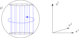
Figure 5: A rigid string beginning and ending on a given $su(2)$ orbit, and rotating.

The motion of the individual endpoints is:

$$\Delta \equiv I_{I}+I_{F}$$

$$I_{I} = \frac{1}{2}e^{-\tau K\Delta}(I_{I}-I_{F})_{0}e^{\tau K\Delta}+\frac{\Delta}{2}$$

$$I_{F} = -\frac{1}{2}e^{-\tau K\Delta}(I_{I}-I_{F})_{0}e^{\tau K\Delta}+\frac{\Delta}{2}$$ (13)

We can also be more explicit about further constraints. Both $I_{I,F}$ should lie in a given sphere since $\langle I_{I},I_{I}\rangle=\langle\lambda_{I},\lambda_{I}\rangle$, and similarly for the final point. This puts constraints on the relation between the initial length vector and the initial velocity, which can be computed. For example, for a fixed orbit $\lambda=\lambda_{I}=\lambda_{F}$ in $SU(2)$ the constraints will say that the stretching of the string (i.e. the relative coordinates of the initial and final points) must be orthogonal to the initial center of mass location, and that the size of the string is fixed in terms of its center of mass coordinate (and the size of the fixed orbit $\lambda$). These constraints can easily be interpreted in the case of $SU(2)$ from the figure 5. Another illustration of a motion in the case of an open string ending on two different orbits is given in figure 6.

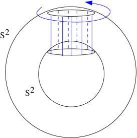
Figure 6: A rigid string stretching between two different $su(2)$ orbits, and rotating.

A check

We would like to check directly that our construction agrees with a limit of the dynamics of open strings on group manifolds as described in string theory. To that end we briefly remind the reader of some aspects of strings on group manifolds (see e.g. [15]). As for the bulk Wess-Zumino-Witten model on group manifolds, the solutions to the classical equations of motion for the open string embedding factorize into a left-moving and a right-moving part:

$$g : \text{strip}\ \mapsto G$$ (14)

$$(\sigma,\tau)\mapsto g(\sigma,\tau)=g_{+}(\sigma+\tau)g_{-}(\sigma-\tau)$$

where the strip is the product of intervals ${[}-\frac{\pi}{2};\frac{\pi}{2}{]}\times\mathbb{R}$. We can define left-moving and right-moving conserved currents:

$$J_{+} = -\partial_{+}g\ g^{-1}$$

$$J_{-} = g^{-1}\partial_{-}g$$ (15)

where we made use of the coordinates $x^{\pm}=\sigma\pm\tau$. The boundary conditions for open strings ending on conjugacy classes [15] are that the left-moving and right-moving current are related by $J_{+}=-J_{-}$ at the endpoints of the open string at $\sigma=\pm\pi/2$. We wish to concentrate on solutions to the open string equations of motion that are rigid (i.e. that have no oscillatory excitations). We thus propose the ansatz:

$$g_{+} = e^{x^{+}T_{+}}g_{+}^{0}$$

$$g_{-} = (g_{-}^{0})^{-1}e^{x^{-}T_{-}}$$ (16)

The boundary conditions then enforce that $T_{+}=T_{-}=T$, where $T$ belongs to the Lie algebra. We thus find the solution to the equations of motion with the boundary conditions (where $g^{0}=g_{+}^{0}(g_{-}^{0})^{-1}$):

$$g(\sigma,\tau)=e^{x^{+}T}g^{0}e^{x^{-}T}=e^{\tau T}(e^{\sigma T}g^{0}e^{\sigma T})e^{-\tau T}$$ (17)

The latter form of the solution shows that every rigid string bit (at fixed value for $\sigma$) moves along its own conjugacy class. In the rigid open string limit of our interest [16], the motion of the string is concentrated near a given point (say, the identity) of the group manifold. We can implement this in the study of our classical solution by assuming that $e^{\sigma T}g^{0}e^{\sigma T}$ is near the identity. By putting $g^{0}=e^{X^{0}}$ and $g=e^{X}$, we get – note when performing the expansion near the identity that the range of $\sigma$ is bounded, while that of $\tau$ is not –:

$$X(\sigma,\tau) = e^{\tau T}(X^{0}+2\sigma T)e^{-\tau T}$$ (18)

It is clear that the two end-points of the open string now behave precisely as in the system described above, namely, they move along orbits in the Lie algebra in accord with the solutions to the equations of motion for our two-particle system. One can identify the parameters $T=K\Delta$, etc. in equations (13) and (18). The comparison to the previous section shows that the charges $I_{I,F}$ are indeed the positions of the endpoints of the string on the Lie algebra. In appendix A we give some further discussion of how the rigid open string limit is taken in Wess-Zumino-Witten models [16].

We also recall here the results of the neat paper [17] (which is based on the intuition for rigid open strings on spheres described in [18]). The paper [17] carefully defines and analyzes the rigid open string limit (for the $SU(2)$ case only) starting from the Wess-Zumino-Witten action for open strings. It shows how in the scaling limit where the volume of the brane is kept fixed, while the bulk is flattened (see appendix A), the action for the open string reduces to an action for two oppositely charged point particles interacting through a spring. The action found in [17] after the limiting procedure coincides with the one we have constructed in equation (8) when restricted to the case of the group $G=SU(2)$. The one-form arises from the electromagnetic field on the D-branes, while the Hamiltonian arises from the bulk length term, and the kinetic term vanishes (as in flat space [14]) in the limit. Now, the verification we performed of the solutions to the equations of motion is equivalent to the analysis of [17] in the $SU(2)$ case, and shows that the limiting procedure on the action generalizes to all groups with a non-degenerate invariant metric.

Thus, we have argued in detail from first principles that our system does describe the classical open string dynamics in the rigid limit. We can thus be confident that the quantization of the system also faithfully represents aspects of quantum mechanical open string theory.

We finally remark that the classical group dynamics that we constructed can be generalized to other systems (not necessarily descending from string theory). It would be interesting to analyze for instance other interaction Hamiltonians (beyond the ”spring Hamiltonian”) consistent with the gauge symmetries of the two-particle system, and to set up the general evaluation of gauge invariant observables (for instance in a path integral formalism). This gives a natural physical context to the extension of the Kirillov formalism from irreducible to tensor product representations.

The rigid open string Hilbert space

Thus far we have mostly discussed the classical rigid open string. We have already observed that the quantum Hilbert space will be a tensor product of irreducible representations $\lambda_{I}\otimes\bar{\lambda_{F}}$. Moreover, the interaction term (proportional to the tension of the string) breaks the $G\times G$ global symmetry to the diagonal subgroup. It is this symmetry breaking that prompts us to decompose the tensor product Hilbert space into representations that are irreducible under the (unbroken diagonal) subgroup. We thus decompose: $\lambda_{I}\otimes\bar{\lambda_{F}}=\sum_{L}{C_{IF}}^{L}\lambda_{L}$ and we interpret the weight $\lambda_{L}$ as being associated to the length of the string (and therefore also to the position of the center of mass of the string). Indeed, note that the conserved quantities classifying the representations will include the quadratic Casimir of the diagonal symmetry group (– which is associated to the conserved charge $\langle I_{I}+I_{F},I_{I}+I_{F}\rangle$ in the classical dynamics –), which is nothing but the length of the string squared. (After quantization this quadratic Casimir is proportional to the conformal weight associated to the vertex operator of the open string state.)

Note that there is a slight change in perspective in the way in which the open string Hilbert space arises here. Were we to quantize the open string ($\sigma$-model) action directly, then the different components of the open string Hilbert space would arise from integrating over all possible lengths $T/K$ of the rigid open string. From the two-particle perspective that we developed, the same open string Hilbert space arises as a tensor product of two single particle Hilbert spaces. After decomposing the tensor product Hilbert space into irreducible representations, we note that the resulting Hilbert spaces coincide.

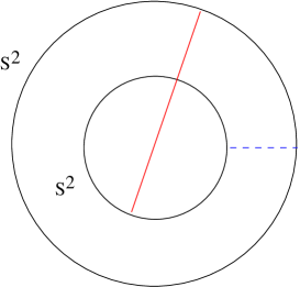
Figure 7: A (blue dashed) string of minimal length and a (red) string of maximal length, stretching between two $su(2)$ orbits.

Returning to our favorite example, the case of $SU(2)$, and fixing for instance that the open string begins and ends on one given D-brane labeled by $j=j_{I}=j_{F}$, we find that we get a decomposition into representations of spins $l=0,1,\dots,2j$ which correspond to a string of length zero up to the maximal extension (root) $2j$. The fact that only integer spins appear follows from the fact that only half-integer spins can appear for a given endpoint, and from the fact that we concentrated on a string that starts and ends on the same brane $j$. The quadratic Casimir will in this case be roughly proportional to the length squared, as is the dimension of the (primary) open string vertex operator : $h_{open}=l(l+1)/(k+2)$. In figure 7 we illustrate a minimal and a maximal length string, in the case of a string ending on two different orbits $j_{I}$ and $j_{F}$ of $su(2)$, with length proportional to $|j_{I}-j_{F}|$ and $j_{I}+j_{F}$ respectively, which correspond to the minimal and maximal spin occurring in the tensor product decomposition $j_{I}\otimes j_{F}$.

Thus, to summarize, we have very general formulas for the semi-classical open string spectrum between any two (symmetric) branes (that correspond to conjugacy classes on group manifolds, or rather, orbits in the Lie algebra), and we understand the quantization in terms of symplectic geometry and geometric quantization. The generality of the formulas follows from our understanding of the quantization of (co-)adjoint orbits. A point that we retain from the semi-classical picture is that the breaking of the product group to the diagonal symmetry group by the open string Hamiltonian gives a physical rationale for decomposing the tensor product representation (since we tend to work in a basis where the Hamiltonian is diagonal).

4 The interactions and a program

4.1 Interactions

We have analyzed the free classical dynamics of open strings, and we have quantized the free string. In the case where we have a finite-dimensional Hilbert space, its dimension is the product of the dimensions of the irreducible representations of which it is the tensor product. (In general, we have a space of linear maps between irreducible Hilbert spaces.) We obtain a $d(\lambda_{I})\times d(\bar{\lambda_{F}})$ matrix representing each string state for an open string stretching between orbits $\lambda_{I,F}$ (where $d(\lambda_{I}),d(\bar{\lambda_{F}})$ denote the dimensions of the representations associated to the weights $\lambda_{I},\bar{\lambda_{F}}$ respectively).

In this section, we turn to the interactions of open strings. Since open strings interact by combining and splitting, which happens when open string endpoints touch, it is natural to assume that open string interactions are coded by the multiplication of the above matrices (or more generally by the composition of linear maps). The final end of a first (oriented) open string will interact with the initial end of a second (oriented) open string.

Figure 8: Concatenating two strings produces a third.

This is the well-known picture that underlies the intuition for open string field theory [19]. See figure 8.

Since the open string interactions are communicated by their endpoints, from the point of view of the center of mass of the open strings, the interactions are non-local. Thus, when the interaction is formulated in terms of the center of mass, we expect to have to take into account an infinite number of derivative terms in coding the interactions. This intuition is familiar from the flat space case clearly explained in [14].

Associativity of the open string interactions will be clear from the associativity of matrix multiplication, or from the associativity of the operation of concatenating open strings. However, when translated in the non-local language adapted to the center of mass of the open string, it is frequently less transparent. We will show later how it is related to non-trivial identities in group theory and the theory of special functions.

The associative product we thus construct is well-known for the case of compact groups, from the analysis of boundary rational conformal field theory, and from the associativity of the boundary vertex operator algebra [5, 20, 21, 22, 23, 24]. For rational conformal field theories, which include Wess-Zumino-Witten models on compact groups, the formulas below are but a toy version of the boundary conformal field theory results. Nevertheless, we will give the explicit description of the formalism, and all precise factors and coefficients for the $SU(2)$ case, since it is instructive, and since we had trouble localizing these simple formulas in the literature in a consistent set of conventions. Moreover, we will show later how this description generalizes to other, non-rational cases that do not fall in the framework of boundary (rational) conformal field theory as developed hitherto.

4.2 A mathematical program

Before we turn to very concrete examples of our construction, we briefly mention an even more general program that we can abstract from the above considerations. We have mostly concentrated on co-adjoint orbits that yield a symplectic foliation of Lie algebras [10]. However, quantization can be applied to much more generic classes of manifolds. We can consider a given Poisson manifold $L$, with four symplectic leaves $M_{1,2,3,4}.$ Let’s suppose that the symplectic form on these leaves is quantizable, and that we can define pre-quantization bundles that admit a good polarization, leading to Hilbert spaces $H_{1,2,3,4}$ corresponding to the manifolds $M_{1,2,3,4}$. Then we can define operators ${O_{i}}^{j}$ which live in the tensor product Hilbert space $H_{i}\otimes\bar{H_{j}}$. The operator product is defined as ${O_{i}}^{j}.{O_{j}}^{k}={O_{i}}^{k}$, where the product is determined by tracing over the middle Hilbert space $H_{j}$. The resulting operation is an associative composition of operators associated to the four Hilbert spaces. It would be interesting to analyze this product generically, and to establish its connection with the analysis of symplectic groupoids. Instead, we delve into a few interesting examples.

5 A compact example: $SU(2)$

In this section, we apply the formalism to the case of the compact Lie group $SU(2)$ in great detail. We develop a diagrammatical language in order to be able to show associativity of the resulting product in terms of group theory.

The kinematical $3j$ symbols

We have argued that we need to decompose the tensor product representation into irreducible representations of the symmetry group. This is a purely kinematical operation from the perspective of open string theory. In order to implement this decomposition, we can choose a basis in the space of matrices (i.e. the tensor product representation) that consists of the Clebsch-Gordan coefficients. Since these are not symmetric under cyclic permutation, we prefer to work with rescaled matrix elements, the $3j$ Wigner symbols. Due to its symmetry properties, we can represent it by a (kinematic) cubic vertex

$$\lower 14.45377pt\hbox{\begin{picture}(0.0,0.0)\includegraphics{3j1.pstex}\end{picture}\begin{picture}(2705.0,1599.0)(3451.0,-4648.0)\put(5026.0,-3511.0){\makebox(0.0,0.0)[lb]{\smash{{{\color[rgb]{0,0,0}$j,-m$}}}}} \put(5326.0,-4261.0){\makebox(0.0,0.0)[lb]{\smash{{{\color[rgb]{0,0,0}$j_{2},m_{2}$}}}}} \put(3451.0,-4261.0){\makebox(0.0,0.0)[lb]{\smash{{{\color[rgb]{0,0,0}$j_{1},m_{1}$}}}}} \end{picture}}=\left(\begin{array}[]{ccc}j_{1}&j_{2}&j\\ m_{1}&m_{2}&-m\end{array}\right)=\frac{(-1)^{j_{1}-j_{2}+m}}{\sqrt{2j+1}}C^{j_{1}\ j_{2}\ j}_{m_{1}m_{2}m}$$ (21)

The explicit formula for the Clebsch-Gordan coefficients reads:

$$C^{j_{1}\ j_{2}\ j}_{m_{1}m_{2}m} = (-1)^{j_{1}+j_{2}-j}\sqrt{2j+1}\sqrt{\frac{(j_{1}-j_{2}+j)!(j_{2}-j_{1}+j)!}{(j_{1}+j_{2}+j+1)!(j_{1}+j_{2}-j)!}}$$ (25)

$$\times\sqrt{\frac{(j_{1}-m_{1})!(j_{2}+m_{2})!(j-m)!(j+m)!}{(j_{1}+m_{1})!(j_{2}-m_{2})!}}$$

$$\times\frac{1}{(j-j_{1}+m_{2})!(j-j_{2}-m_{1})!}$$

$$\times{{}_{3}}F_{2}\left(\begin{array}[]{c}j-j_{1}-j_{2},\ \ -j_{1}-m_{1},\ \ -j_{2}+m_{2}\\ j-j_{1}+m_{2}+1,\ \ j-j_{2}-m_{1}+1\end{array};1\right)$$

In our conventions, $j_{i}$ and $m_{i}$ are half-integers, with $j_{i}$ positive and $-j_{i}~{}\leq~{}m_{i}~{}\leq~{}j_{i}$. Moreover, $m_{1}+m_{2}-m=0$ and $|j_{1}-j_{2}|\leq j\leq j_{1}+j_{2}$. If these conditions are not satisfied, the Clebsch-Gordan coefficient is zero. Note that conservation of the quantum number $m$ can be read very easily from our diagrammatic notation. The dimension of the $SU(2)$ representation is $2j_{i}+1$ and the Casimir is $j_{i}(j_{i}+1)$. A useful reference for Clebsch-Gordan and Racah coefficients (or equivalently 3j and 6j Wigner symbols) of the $SU(2)$ group is [26].

One remark should be made concerning the arrows that appear in our diagrammatic notation, since their direction does matter. More precisely, changing the direction of an arrow amounts to multiplying the vertex by a propagator which is the 1j Wigner symbol introduced in [27]:

$$\lower 7.22743pt\hbox{\begin{picture}(0.0,0.0)\includegraphics{1j1.pstex}\end{picture}\begin{picture}(1143.0,666.0)(5992.0,-4019.0)\put(6151.0,-3961.0){\makebox(0.0,0.0)[lb]{\smash{{{\color[rgb]{0,0,0}$m$}}}}} \put(6451.0,-3511.0){\makebox(0.0,0.0)[lb]{\smash{{{\color[rgb]{0,0,0}$j$}}}}} \put(6601.0,-3961.0){\makebox(0.0,0.0)[lb]{\smash{{{\color[rgb]{0,0,0}$m^{\prime}$}}}}} \end{picture}}=(-1)^{j+m}\ \delta_{m,-m^{\prime}}=(-1)^{j-m^{\prime}}\ \delta_{m,-m^{\prime}}$$ (26)

Although simply a sign in the case of $SU(2)$, it can become more complicated for other groups. For instance, we have:

(29)

$$= \ \left(\begin{array}[]{ccc}j_{1}&j_{2}&j\\ m_{1}&m_{2}&-m\end{array}\right)\ \lower 10.84006pt\hbox{\begin{picture}(0.0,0.0)\includegraphics{1j2.pstex}\end{picture}\begin{picture}(1068.0,657.0)(5992.0,-4010.0)\put(6451.0,-3511.0){\makebox(0.0,0.0)[lb]{\smash{{{\color[rgb]{0,0,0}$j$}}}}} \put(6151.0,-3961.0){\makebox(0.0,0.0)[lb]{\smash{{{\color[rgb]{0,0,0}$-m$}}}}} \put(6676.0,-3961.0){\makebox(0.0,0.0)[lb]{\smash{{{\color[rgb]{0,0,0}$m$}}}}} \end{picture}}$$ (32)

while for changing the direction of the $j_{1}$ arrow, one would have to multiply the 3j symbol by $(-1)^{j_{1}+m_{1}}$.

Another remark is that the overall inward direction we chose for arrows in $(\ref{3jdef})$ was arbitrary:

$$\lower 14.45377pt\hbox{\begin{picture}(0.0,0.0)\includegraphics{3j1.pstex}\end{picture}\begin{picture}(2705.0,1599.0)(3451.0,-4648.0)\put(5026.0,-3511.0){\makebox(0.0,0.0)[lb]{\smash{{{\color[rgb]{0,0,0}$j,-m$}}}}} \put(5326.0,-4261.0){\makebox(0.0,0.0)[lb]{\smash{{{\color[rgb]{0,0,0}$j_{2},m_{2}$}}}}} \put(3451.0,-4261.0){\makebox(0.0,0.0)[lb]{\smash{{{\color[rgb]{0,0,0}$j_{1},m_{1}$}}}}} \end{picture}}\hskip 5.69046pt=\ \lower 14.45377pt\hbox{\begin{picture}(0.0,0.0)\includegraphics{3j2.pstex}\end{picture}\begin{picture}(2705.0,1599.0)(3451.0,-4648.0)\put(3451.0,-4261.0){\makebox(0.0,0.0)[lb]{\smash{{{\color[rgb]{0,0,0}$j_{1},m_{1}$}}}}} \put(5026.0,-3511.0){\makebox(0.0,0.0)[lb]{\smash{{{\color[rgb]{0,0,0}$j,-m$}}}}} \put(5326.0,-4261.0){\makebox(0.0,0.0)[lb]{\smash{{{\color[rgb]{0,0,0}$j_{2},m_{2}$}}}}} \end{picture}}$$ (33)

i.e one may as well choose to represent the 3j symbol by a vertex with all arrows pointing outwards.

We now recall, in our diagrammatic notation, several important results for 3j symbols. Our notation immediately reflects their invariance under circular permutation of its indices. Beside cyclic permutation, two other useful symmetry properties of the 3j symbols are:

(34)

$$= \ (-1)^{j_{1}+j_{2}+j}\ \ \lower 14.45377pt\hbox{\begin{picture}(0.0,0.0)\includegraphics{3j5.pstex}\end{picture}\begin{picture}(2705.0,1599.0)(3451.0,-4648.0)\put(5026.0,-3511.0){\makebox(0.0,0.0)[lb]{\smash{{{\color[rgb]{0,0,0}$j,-m$}}}}} \put(3451.0,-4261.0){\makebox(0.0,0.0)[lb]{\smash{{{\color[rgb]{0,0,0}$j_{2},m_{2}$}}}}} \put(5326.0,-4261.0){\makebox(0.0,0.0)[lb]{\smash{{{\color[rgb]{0,0,0}$j_{1},m_{1}$}}}}} \end{picture}}$$ (35)

Note that permuting any two branches, whatever the direction of the arrows, always amounts to a multiplication by $(-1)^{j_{1}+j_{2}+j}$, while $(\ref{3jchangem})$ is only true when all arrows point inwards or outwards, otherwise extra signs appear due to 1j symbols.

In the following we will concatenate 3j symbols – concatenation is possible when arrow directions are aligned and the labels $j_{i},m_{i}$ coincide. Concatenation implies that we sum over all internal half-integers $m_{i}$. The sums will always be finite since only a finite number of 3j symbols are non-zero.

The 3j symbols satisfy orthogonality and completeness relations:

$$\lower 28.90755pt\hbox{\begin{picture}(0.0,0.0)\includegraphics{normalization1.pstex}\end{picture}\begin{picture}(3565.0,2424.0)(4276.0,-5173.0)\put(4276.0,-4036.0){\makebox(0.0,0.0)[lb]{\smash{{{\color[rgb]{0,0,0}$j_{1}$}}}}} \put(7426.0,-4036.0){\makebox(0.0,0.0)[lb]{\smash{{{\color[rgb]{0,0,0}$j_{2}$}}}}} \put(6151.0,-3436.0){\makebox(0.0,0.0)[lb]{\smash{{{\color[rgb]{0,0,0}$j^{\prime},m^{\prime}$}}}}} \put(6151.0,-4786.0){\makebox(0.0,0.0)[lb]{\smash{{{\color[rgb]{0,0,0}$j,m$}}}}} \end{picture}}=\lower 36.135pt\hbox{\begin{picture}(0.0,0.0)\includegraphics{normalization2.pstex}\end{picture}\begin{picture}(1840.0,2424.0)(8476.0,-5173.0)\put(9901.0,-3961.0){\makebox(0.0,0.0)[lb]{\smash{{{\color[rgb]{0,0,0}$j_{2}$}}}}} \put(9451.0,-4861.0){\makebox(0.0,0.0)[lb]{\smash{{{\color[rgb]{0,0,0}$j,m$}}}}} \put(9451.0,-3136.0){\makebox(0.0,0.0)[lb]{\smash{{{\color[rgb]{0,0,0}$j^{\prime},m^{\prime}$}}}}} \put(8476.0,-3961.0){\makebox(0.0,0.0)[lb]{\smash{{{\color[rgb]{0,0,0}$j_{1}$}}}}} \end{picture}}=\ \frac{(-1)^{j_{1}+j_{2}+j}}{2j+1}\ \delta_{j,j^{\prime}}\ \delta_{m,m^{\prime}}$$ (38)

and

$$\sum_{j}\ (2j+1)\ \ \lower 14.45377pt\hbox{\begin{picture}(0.0,0.0)\includegraphics{normalization3.pstex}\end{picture}\begin{picture}(3375.0,1270.0)(4576.0,-4619.0)\put(4576.0,-4561.0){\makebox(0.0,0.0)[lb]{\smash{{{\color[rgb]{0,0,0}$j_{2},m_{2}$}}}}} \put(4576.0,-3511.0){\makebox(0.0,0.0)[lb]{\smash{{{\color[rgb]{0,0,0}$j_{1},m_{1}$}}}}} \put(7951.0,-3511.0){\makebox(0.0,0.0)[lb]{\smash{{{\color[rgb]{0,0,0}$j_{2},m_{2}^{\prime}$}}}}} \put(6451.0,-3736.0){\makebox(0.0,0.0)[lb]{\smash{{{\color[rgb]{0,0,0}$j$}}}}} \put(7951.0,-4486.0){\makebox(0.0,0.0)[lb]{\smash{{{\color[rgb]{0,0,0}$j_{1},m_{1}^{\prime}$}}}}} \end{picture}}\hskip 22.76228pt=\delta_{m_{1},m_{1}^{\prime}}\ \delta_{m_{2},m_{2}^{\prime}}$$ (39)

The dynamical $6j$ symbols

We now recall some useful results concerning the 6j Wigner symbol. It can be expressed in terms of four Clebsch-Gordan coefficients:

$$\left\{\begin{array}[]{ccc}j_{1}&j_{2}&j_{12}\\ j_{3}&j&j_{23}\end{array}\right\}\ =\ \frac{(-1)^{j_{1}+j_{2}+j_{3}+j}}{\sqrt{(2j_{12}+1)(2j_{23}+1)}(2j+1)}$$ (42)

$$\hskip 42.67912pt\times\sum_{m_{1},m_{2},m_{3}\in\frac{1}{2}\mathbb{N}}C^{j_{1}\ j_{2}\ j_{12}}_{m_{1}m_{2}m_{12}}\ C^{j_{12}\ j_{3}\ j}_{m_{12}m_{3}m}\ C^{j_{2}\ j_{3}\ j_{23}}_{m_{2}m_{3}m_{23}}\ C^{j_{1}\ j_{23}\ j}_{m_{1}m_{23}m}$$

In terms of 1j and 3j symbols, in our diagrammatic notation, $(\ref{6j43j})$ is simply:

$$\left\{\begin{array}[]{ccc}j_{1}&j_{2}&j_{12}\\ j_{3}&j&j_{23}\end{array}\right\}\ =\ \lower 28.90755pt\hbox{\begin{picture}(0.0,0.0)\includegraphics{6j1.pstex}\end{picture}\begin{picture}(3340.0,2793.0)(3151.0,-5173.0)\put(3151.0,-4411.0){\makebox(0.0,0.0)[lb]{\smash{{{\color[rgb]{0,0,0}$j_{1}$}}}}} \put(6076.0,-4336.0){\makebox(0.0,0.0)[lb]{\smash{{{\color[rgb]{0,0,0}$j_{2}$}}}}} \put(4951.0,-4561.0){\makebox(0.0,0.0)[lb]{\smash{{{\color[rgb]{0,0,0}$j_{12}$}}}}} \put(5176.0,-3886.0){\makebox(0.0,0.0)[lb]{\smash{{{\color[rgb]{0,0,0}$j_{3}$}}}}} \put(4201.0,-3886.0){\makebox(0.0,0.0)[lb]{\smash{{{\color[rgb]{0,0,0}$j$}}}}} \put(4576.0,-2536.0){\makebox(0.0,0.0)[lb]{\smash{{{\color[rgb]{0,0,0}$j_{23}$}}}}} \end{picture}}$$ (45)

The 6j symbol has a large group of symmetry, consisting of 144 elements and generated by the transformations:

$$(1)\ \left\{\begin{array}[]{l}j_{1}\leftrightarrow j_{2}\\ j_{3}\leftrightarrow j\end{array}\right.\ \ \hskip 28.45274pt(2)\ \left\{\begin{array}[]{l}j_{1}\leftrightarrow j_{12}\\ j_{3}\leftrightarrow j_{23}\end{array}\right.$$ , (50)

$$(3)\ \left\{\begin{array}[]{l}j_{1}\leftrightarrow j_{3}\\ j_{2}\leftrightarrow j\end{array}\right.\ \ \hskip 28.45274pt(4)\ \left\{\begin{array}[]{l}j_{1,2,3}\rightarrow l-j_{1,2,3}\\ j\rightarrow l-j\end{array}\right.$$ , (55)

where $l=\frac{1}{2}(j_{1}+j_{2}+j_{3}+j)$. The 6j symbol is invariant under any of these transformations, therefore under any permutation of its columns. An interesting well-known remark is that this group of symmetries includes the symmetries of a tetrahedron [27],

Figure 9: The 6j symbol as a tetrahedron.

i.e one should see our planar representation of the 6j symbol $(\ref{6jplanar})$ as a projection of the tetrahedron pictured in $(\ref{tetrahedron})$ on the plane $BCD$ (with properly added arrows). From this representation, it is clear that the result should be invariant of which tip of the tetrahedron is used in order to project and obtain a planar diagram. To be more precise, the symmetries of the tetrahedron generate transformations (1), (2) and (3) (but not transformation (4)), with the following correspondence:

• transformation (1) $\longleftrightarrow$ invert and project from tip A

• transformation (2) $\longleftrightarrow$ invert and project from tip B

• transformation (3) $\longleftrightarrow$ project from tip C

• transformation (1), then (2) $\longleftrightarrow$ project from tip D

where inverting the tetrahedron means that we take its mirror image with respect to the plane opposite to the tip which we will project.

In the following we will need two important formulas. The first one is the recoupling identity, which can be seen as a toy s-channel - t-channel duality:

(57)

This identity originates from the definition of the $3j$ and $6j$ symbols as transformations of bases. It is worth noting that this identity together with the orthogonality relation $(\ref{jmnormal})$ implies formula $(\ref{6j43j})$ for the $6j$ symbol. We will also need the Biedenharn-Elliott identity (which follows from the associativity of the tensor product of representations):

$$\sum_{j_{23}\in\frac{1}{2}\mathbb{N}}(2j_{23}+1)(-1)^{J} j_{1} j_{2} j_{12} j_{3} j_{23} j_{123} j_{1} j_{234} j_{4} j_{123} j_{23} j j_{34} j_{4} j_{3} j_{23} j_{2} j_{234}$$ (58)

$$=\lower 21.68121pt\hbox{\begin{picture}(0.0,0.0)\includegraphics{biedenharn4.pstex}\end{picture}\begin{picture}(3415.0,2793.0)(3076.0,-5173.0)\put(4576.0,-2536.0){\makebox(0.0,0.0)[lb]{\smash{{{\color[rgb]{0,0,0}$j_{34}$}}}}} \put(5176.0,-3886.0){\makebox(0.0,0.0)[lb]{\smash{{{\color[rgb]{0,0,0}$j_{4}$}}}}} \put(6076.0,-4336.0){\makebox(0.0,0.0)[lb]{\smash{{{\color[rgb]{0,0,0}$j_{3}$}}}}} \put(4951.0,-4561.0){\makebox(0.0,0.0)[lb]{\smash{{{\color[rgb]{0,0,0}$j_{123}$}}}}} \put(4201.0,-3886.0){\makebox(0.0,0.0)[lb]{\smash{{{\color[rgb]{0,0,0}$j$}}}}} \put(3076.0,-4411.0){\makebox(0.0,0.0)[lb]{\smash{{{\color[rgb]{0,0,0}$j_{12}$}}}}} \end{picture}}\ \lower 21.68121pt\hbox{\begin{picture}(0.0,0.0)\includegraphics{biedenharn5.pstex}\end{picture}\begin{picture}(3340.0,2793.0)(3151.0,-5173.0)\put(4201.0,-3886.0){\makebox(0.0,0.0)[lb]{\smash{{{\color[rgb]{0,0,0}$j$}}}}} \put(4576.0,-2536.0){\makebox(0.0,0.0)[lb]{\smash{{{\color[rgb]{0,0,0}$j_{234}$}}}}} \put(5176.0,-3886.0){\makebox(0.0,0.0)[lb]{\smash{{{\color[rgb]{0,0,0}$j_{34}$}}}}} \put(4951.0,-4561.0){\makebox(0.0,0.0)[lb]{\smash{{{\color[rgb]{0,0,0}$j_{12}$}}}}} \put(6076.0,-4336.0){\makebox(0.0,0.0)[lb]{\smash{{{\color[rgb]{0,0,0}$j_{2}$}}}}} \put(3151.0,-4411.0){\makebox(0.0,0.0)[lb]{\smash{{{\color[rgb]{0,0,0}$j_{1}$}}}}} \end{picture}}$$

where $J=j_{1}+j_{2}+j_{3}+j_{4}+j+j_{12}+j_{23}+j_{34}+j_{123}+j_{234}$. One last useful formula can be obtained from the recoupling identity $(\ref{recouplingid})$ and the orthogonality property $(\ref{jmnormal})$ and reads:

$$\lower 21.68121pt\hbox{\begin{picture}(0.0,0.0)\includegraphics{6j3.pstex}\end{picture}\begin{picture}(3980.0,2649.0)(301.0,-5098.0)\put(3451.0,-4711.0){\makebox(0.0,0.0)[lb]{\smash{{{\color[rgb]{0,0,0}$j_{2},m_{2}$}}}}} \put(2251.0,-4861.0){\makebox(0.0,0.0)[lb]{\smash{{{\color[rgb]{0,0,0}$j_{23}$}}}}} \put(3226.0,-3961.0){\makebox(0.0,0.0)[lb]{\smash{{{\color[rgb]{0,0,0}$j_{3}$}}}}} \put(1426.0,-3961.0){\makebox(0.0,0.0)[lb]{\smash{{{\color[rgb]{0,0,0}$j$}}}}} \put(2551.0,-2911.0){\makebox(0.0,0.0)[lb]{\smash{{{\color[rgb]{0,0,0}$j_{12},m_{12}$}}}}} \put(301.0,-4711.0){\makebox(0.0,0.0)[lb]{\smash{{{\color[rgb]{0,0,0}$j_{1},m_{1}$}}}}} \end{picture}}=(-1)^{j_{1}-j_{2}+j_{12}+2j}\lower 21.68121pt\hbox{\begin{picture}(0.0,0.0)\includegraphics{6j4.pstex}\end{picture}\begin{picture}(3340.0,2793.0)(3151.0,-5173.0)\put(3151.0,-4411.0){\makebox(0.0,0.0)[lb]{\smash{{{\color[rgb]{0,0,0}$j_{1}$}}}}} \put(6076.0,-4336.0){\makebox(0.0,0.0)[lb]{\smash{{{\color[rgb]{0,0,0}$j_{2}$}}}}} \put(4951.0,-4561.0){\makebox(0.0,0.0)[lb]{\smash{{{\color[rgb]{0,0,0}$j_{12}$}}}}} \put(5176.0,-3886.0){\makebox(0.0,0.0)[lb]{\smash{{{\color[rgb]{0,0,0}$j_{3}$}}}}} \put(4201.0,-3886.0){\makebox(0.0,0.0)[lb]{\smash{{{\color[rgb]{0,0,0}$j$}}}}} \put(4576.0,-2536.0){\makebox(0.0,0.0)[lb]{\smash{{{\color[rgb]{0,0,0}$j_{23}$}}}}} \end{picture}}\ \ \lower 21.68121pt\hbox{\begin{picture}(0.0,0.0)\includegraphics{3j6.pstex}\end{picture}\begin{picture}(2959.0,1599.0)(3451.0,-4648.0)\put(5326.0,-4261.0){\makebox(0.0,0.0)[lb]{\smash{{{\color[rgb]{0,0,0}$j_{2},m_{2}$}}}}} \put(3451.0,-4261.0){\makebox(0.0,0.0)[lb]{\smash{{{\color[rgb]{0,0,0}$j_{1},m_{1}$}}}}} \put(5026.0,-3511.0){\makebox(0.0,0.0)[lb]{\smash{{{\color[rgb]{0,0,0}$j_{12},m_{12}$}}}}} \end{picture}}$$ (59)

Associativity

We now code the interaction of open strings, which is the matrix product, in terms of our diagrammatic notation. Multiplication of matrices corresponds to concatenating diagrams, with the convention that internal lines are summed over. We then compute the cubic rigid string interaction vertex, which is a dynamical quantity. We indicate the different nature of the cubic vertex from the kinematical one by color-coding: bold blue branches indicate centers of mass (spin $l_{i}$), while black branches indicate branes (spin $j_{i}$).

A string stretching between two $SU(2)$ orbits labeled by their spins $j_{1}$ and $j_{2}$ respectively, with its center of mass in the representation $l$, will be represented by the following matrix elements:

$$\left[\Theta^{l}_{m}\right]^{j_{1}j_{2}}_{n_{1}n_{2}}=\lower 14.45377pt\hbox{\begin{picture}(0.0,0.0)\includegraphics{3j7.pstex}\end{picture}\begin{picture}(2659.0,1620.0)(3451.0,-4648.0)\put(3451.0,-4261.0){\makebox(0.0,0.0)[lb]{\smash{{{\color[rgb]{0,0,0}$j_{1},n_{1}$}}}}} \put(5326.0,-4261.0){\makebox(0.0,0.0)[lb]{\smash{{{\color[rgb]{0,0,0}$j_{2},n_{2}$}}}}} \put(5026.0,-3511.0){\makebox(0.0,0.0)[lb]{\smash{{{\color[rgb]{0,0,0}$l,-m$}}}}} \end{picture}}$$ (60)

Figure 10: Two strings interacting.

Two strings may interact if their endpoints move in the same $SU(2)$ orbits, see figure 10. This interaction is encoded in the multiplication of the associated matrices, which can be decomposed as a sum:

$$\left[\Theta^{l_{1}}_{m_{1}}\right]^{j_{1}j_{2}}_{n_{1}n_{2}}\times\left[\Theta^{l_{2}}_{m_{2}}\right]^{j_{2}j_{3}}_{n_{2}n_{3}}=\sum_{l_{12},m_{12}\in\frac{1}{2}\mathbb{N}}c_{l_{12},m_{12}}\left[\Theta^{l_{12}}_{m_{12}}\right]^{j_{1}j_{3}}_{n_{1}n_{3}}$$ (61)

where $l_{12}$ is a representation in the tensor product of $l_{1}$ and $l_{2}$, and where the coefficient $c_{l_{12},m_{12}}$ can be computed using $(\ref{3jinteraction})$ and $(\ref{jmnormal})$:

$$c_{l_{12},m_{12}}=(-1)^{\alpha_{c}}\ (2l_{12}+1)\ \lower 21.68121pt\hbox{\begin{picture}(0.0,0.0)\includegraphics{6j5.pstex}\end{picture}\begin{picture}(3340.0,2814.0)(3151.0,-5194.0)\put(6076.0,-4336.0){\makebox(0.0,0.0)[lb]{\smash{{{\color[rgb]{0,0,0}$j_{3}$}}}}} \put(4576.0,-2536.0){\makebox(0.0,0.0)[lb]{\smash{{{\color[rgb]{0,0,0}$j_{2}$}}}}} \put(3151.0,-4411.0){\makebox(0.0,0.0)[lb]{\smash{{{\color[rgb]{0,0,0}$j_{1}$}}}}} \put(3976.0,-3811.0){\makebox(0.0,0.0)[lb]{\smash{{{\color[rgb]{0,0,1}$l_{1}$}}}}} \put(5251.0,-3811.0){\makebox(0.0,0.0)[lb]{\smash{{{\color[rgb]{0,0,1}$l_{2}$}}}}} \put(5026.0,-4636.0){\makebox(0.0,0.0)[lb]{\smash{{{\color[rgb]{0,0,1}$l_{12}$}}}}} \end{picture}}\ \ \lower 14.45377pt\hbox{\begin{picture}(0.0,0.0)\includegraphics{3j8.pstex}\end{picture}\begin{picture}(2809.0,1641.0)(4801.0,-4669.0)\put(4801.0,-4261.0){\makebox(0.0,0.0)[lb]{\smash{{{\color[rgb]{0,0,1}$l_{1},m_{1}$}}}}} \put(6526.0,-4261.0){\makebox(0.0,0.0)[lb]{\smash{{{\color[rgb]{0,0,1}$l_{2},m_{2}$}}}}} \put(6226.0,-3511.0){\makebox(0.0,0.0)[lb]{\smash{{{\color[rgb]{0,0,1}$l_{12},m_{12}$}}}}} \end{picture}}$$ (62)

where $\alpha_{c}=j_{1}+j_{3}+2l_{2}-l_{12}$ (See e.g. [28, 16] for earlier occurrences of this product for the case of a fixed orbit $j$). Now that we have the interaction vertex, and therefore the product of open string operators, we can check associativity for the string interaction directly in this non-local formalism (instead of using the map to the multiplication of matrices). The proof of the associativity of the product reads:

$$\left(\left[\Theta^{l_{1}}_{m_{1}}\right]^{j_{1}j_{2}}_{n_{1}n_{2}}\times\left[\Theta^{l_{2}}_{m_{2}}\right]^{j_{2}j_{3}}_{n_{2}n_{3}}\right)\times\left[\Theta^{l_{3}}_{m_{3}}\right]^{j_{3}j_{4}}_{n_{3}n_{4}}$$

$$\hskip 56.9055pt=\sum_{l_{12},m_{12}}c_{l_{12},m_{12}}\left[\Theta^{l_{12}}_{m_{12}}\right]^{j_{1}j_{3}}_{n_{1}n_{3}}\times\left[\Theta^{l_{3}}_{m_{3}}\right]^{j_{3}j_{4}}_{n_{3}n_{4}}$$ (63)

$$=\sum_{l_{12},l}\ (-1)^{2j_{1}+j_{3}+j_{4}+2l_{2}+2l_{3}-l_{12}-l}(2l_{12}+1)(2l+1)$$

(64)

$$=\sum_{l_{12},l}\ (-1)^{2j_{1}+j_{3}+j_{4}-l_{12}-l_{2}-l_{3}+l_{1}-2l}(2l_{12}+1)(2l_{23}+1)(2l+1)$$

(65)

$$=\sum_{l_{23},l}\ (-1)^{j_{1}+j_{2}+2j_{4}+2l_{3}-l_{23}-l}(2l_{23}+1)(2l+1)$$

(66)

$$=\sum_{l_{23},m_{23}}c_{l_{23},m_{23}}\left[\Theta^{l_{1}}_{m_{1}}\right]^{j_{1}j_{2}}_{n_{1}n_{2}}\times\left[\Theta^{l_{23}}_{m_{23}}\right]^{j_{2}j_{4}}_{n_{2}n_{4}}$$

$$=\left[\Theta^{l_{1}}_{m_{1}}\right]^{j_{1}j_{2}}_{n_{1}n_{2}}\times\left(\left[\Theta^{l_{2}}_{m_{2}}\right]^{j_{2}j_{3}}_{m_{2}m_{3}}\times\left[\Theta^{l_{3}}_{m_{3}}\right]^{j_{3}j_{4}}_{m_{3}m_{4}}\right)$$ (67)

We have used the recoupling identity $(\ref{recoupling})$ to go from $(\ref{assoc1})$ to $(\ref{assoc2})$ and the Biedenharn-Elliott identity $(\ref{biedenharn})$ to go from $(\ref{assoc2})$ to $(\ref{assoc3})$. The proof is very general. In particular, it generalizes the diagrammatic proof of [25] to the case of differing initial and final orbits. It only makes use of generic properties of groups like associativity of the tensor product composition. We will thus be able to show that it applies to cases not considered before in the literature.

The relation to (rational) boundary conformal field theory

The diagrammar above can be viewed as a special case of the work of [22, 23] (and follow-ups) on the algebra of boundary conformal field theories. Our diagrams and diagrammatic techniques are (for the case of $SU(2)$) semi-classical limits of the analysis done in these papers for rational conformal field theories.

The fact that group theory forms a representation of classical chiral conformal field theory data has been known since the seminal work [5] on axioms of conformal field theory. (The 3j symbols correspond to intertwiners and the 6j symbols to fusion matrices.) However, it has almost exclusively been applied to finite, or compact groups, and to rational conformal field theories. A notable exception is the treatment of the $H_{4}$ group in [29, 30]. Also, a physical situation to which the classical limit applies was left undetermined in [5] as well as in many other works on realizations of chiral conformal field theory data. In particular, it was already noticed in the work [5] that the classical limit of chiral conformal field theory would not be applicable to bulk quantities like the torus partition function. Presently, this is understood from the fact that the chiral conformal field theory data may be thought off as applying to open string dynamics, and that the bulk theory flattens to a Lie algebra (of infinite volume).

We believe the simple model we developed gives a neat physical picture of all the relevant ingredients, even illuminating the (well-known) formulas of the compact case. That this extra intuition is useful will become clear in the following. Indeed, our construction works for any group, including non-compact groups. This implies in particular that we can treat the semi-classical limit of models that fall outside the framework of rational conformal field theory considered in [22, 23] (see also [5, 20, 21, 24]).

Note that it is traditional to represent the matrices $\Theta_{m}^{l}$ as matrix elements of the corresponding spherical functions. In this way, one obtains an associative product of spherical functions (see equation (62)). If we concentrate on a fixed brane and the open strings living on it, we obtain the fuzzy sphere function algebra [28, 31]. This point is further discussed in the appendix B. Note that this construction generalizes easily to a function algebra for spherical functions associated to different orbits, and to the case of spherical functions on generic orbits (or flag manifolds). All these function algebras are associative and non-commutative.

We have already given explicit formulas for the compact case of $S^{2}$ branes associated to $SU(2)$. Let us now proceed to produce new results for the rigid open string limit of non-compact branes associated to $SL(2,\mathbb{R})$ in order the illustrate the utility of our approach. We will first give a geometric description of the orbits, of the tensor product and of the interactions, then we will produce explicit results.

6 Remarks on $SL(2,\mathbb{R})$ orbits and products

In this section we develop our intuition on the kind of string interactions that we will describe in section 7 when we will analyze associative products associated to $SL(2,\mathbb{R})$ orbits .

6.1 Orbits and representations

The co-adjoint orbits of $SL(2,\mathbb{R})$ are given in figure 11. Vectors representing strings can be drawn between these orbits (with their endpoints lying on the orbits), like in figure 12 or 13 for instance. We have therefore future and past time-like and light-like vectors, and space-like vectors. The time-like vectors correspond to discrete representations while the continuous representations correspond to space-like vectors (see e.g. [11] for a detailed discussion of the correspondence).

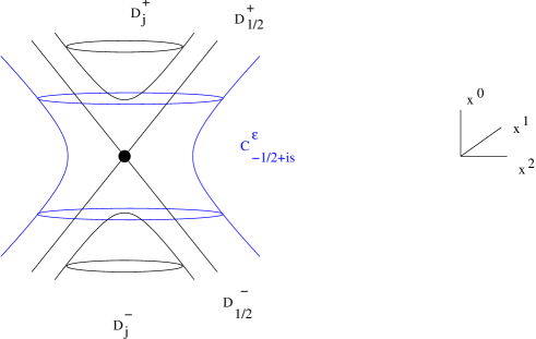
Figure 11: The $sl(2,\mathbb{R})$ co-adjoint orbits. One-sheeted hyperboloids correspond to continuous representations and two-sheeted hyperboloids to discrete representations (the upper sheet being associated to positive discrete representations and the lower sheet to negative ones). The future and past light-cone (with the point at the origin removed) correspond to the special cases of discrete representations with $j=\frac{1}{2}$ while the point at the origin represents the trivial (identity) representation.

Moreover, consider for instance a space-like oriented string which starts and ends on a given (positive) discrete orbit (see figure 13). Its first endpoint which is a positively charged particle is then associated to a lowest weight representation and its negatively charged second endpoint is associated to a highest weight representation. Indeed, recall that we had to consider the tensor product $\lambda_{I}\otimes\bar{\lambda}_{F}$. There are strings corresponding to any tensor product combination.

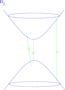
Figure 12: Some past time-like strings starting on a future discrete orbit and ending on a past discrete orbit.

6.2 The geometry of tensor product decomposition

To understand the irreducible representations in which the center-of-mass wave-functions transform, we take a closer look at the tensor product decompositions of $SL(2,\mathbb{R})$ representations [32]:

$$\mathcal{D}^{\pm}_{j_{1}}\otimes\mathcal{D}^{\pm}_{j_{2}} = \oplus_{j\geq j_{1}+j_{2}}\mathcal{D}^{\pm}_{j}$$ (68)

$$\mathcal{D}^{+}_{j_{1}}\otimes\mathcal{D}^{-}_{j_{2}} = \int_{0}^{\infty}ds\ \mathcal{C}^{\epsilon}_{s}+\Theta(j_{1}-j_{2}-1)\oplus_{j=j_{\text{min}}}^{j_{1}-j_{2}}\mathcal{D}^{+}_{j}$$

$$\hskip 42.67912pt+\Theta(j_{2}-j_{1}-1)\oplus_{j=j_{\text{min}}}^{j_{2}-j_{1}}\mathcal{D}^{-}_{j}$$

$$\hskip 28.45274pt\text{where}\ \epsilon=0,\ j_{\text{min}}=1\ \text{if}\ j_{1}+j_{2}\ \text{is integer}$$

$$\hskip 28.45274pt\text{and}\ \epsilon=\frac{1}{2}\ ,\ j_{\text{min}}=\frac{3}{2}\ \text{otherwise}$$

$$\mathcal{D}^{\pm}_{j_{1}}\otimes\mathcal{C}^{\epsilon_{2}}_{s_{2}} = \int_{0}^{\infty}ds\ \mathcal{C}^{\epsilon}_{s}\oplus_{j\geq j_{\text{min}}}\mathcal{D}_{j}^{\pm}$$

$$\hskip 28.45274pt\text{where}\ \epsilon=0,\ j_{\text{min}}=1\ \text{if}\ j_{1}+\epsilon_{2}\ \text{is integer}$$

$$\hskip 28.45274pt\text{and}\ \epsilon=\frac{1}{2}\ ,\ j_{\text{min}}=\frac{3}{2}\ \text{otherwise}$$

$$\mathcal{C}^{\epsilon_{1}}_{s_{1}}\otimes\mathcal{C}^{\epsilon_{2}}_{s_{2}} = \oplus_{j\geq j_{\text{min}}}\mathcal{D}_{j}^{+}\oplus_{j\geq j_{\text{min}}}\mathcal{D}_{j}^{-}\oplus 2\int_{0}^{\infty}ds\ \mathcal{C}^{\epsilon}_{s}$$

$$\hskip 28.45274pt\text{where}\ \epsilon=0,\ j_{\text{min}}=1\ \text{if}\ \epsilon_{1}+\epsilon_{2}\ \text{is integer}$$

$$\hskip 28.45274pt\text{and}\ \epsilon=\frac{1}{2}\ ,\ j_{\text{min}}=\frac{3}{2}\ \text{otherwise}$$

where generically $j_{i}$ is a half-integer verifying $j_{i}\geq\frac{1}{2}$, $\epsilon_{i}=0$ or $\frac{1}{2}$ and $0<s_{i}<\infty$. The function $\Theta(x)$ is the Heaviside function that gives $1$ if $x\geq 0$ and $0$ otherwise. We have seen in the previous sections that we should be able to interpret this tensor product decomposition geometrically. Namely, the possible difference vectors (within the vector space that is the Lie algebra) of the positions of the open string stretching between two orbits are associated to representatives of orbits that give rise to representations appearing in the tensor product decomposition. Let us give an approximate discussion of how this is consistent with the above list.

• If we take a past time-like vector and a future time-like vector, then the difference is a past time-like vector. Its minimal length depends on the minimal lengths of these vectors linearly. That explains the first relation in (68). See figure 12.

• The difference of two future time-like vectors can give either a space-like vector (see figure 13), or depending on their relative length, a future time-like or a past time-like vector. That geometry corresponds to the second relation in (68).

• The difference of a future time-like vector and a space-like vector either gives a space-like vector, or a future time-like vector. See the third relation in (68).

• The difference of two space-like vectors can take any form, as the tensor product in the last line in (68).

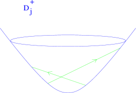
Figure 13: A few space-like strings starting and ending on a given discrete orbit.

This list is a rather sketchy explanation of the tensor product decompositions, but we hope it is clear that the correspondence of the representation theory and the geometric (quantization) picture can be made precise.

6.3 Interactions

Since there are many sorts of (rigid open) strings we can realize associative products arising from string concatenation in many different spaces. In the following section we will concentrate on a very particular case, for simplicity, although the construction is generic for all discrete and continuous representations.

Let us consider the possibility where all the representations involved are discrete representations. We can consider an open string stretching from a (upward oriented) discrete orbit to another (upward oriented) discrete orbit, corresponding to a tensor product representation $\mathcal{D}^{+}_{j_{1}}\otimes\mathcal{D}^{-}_{j_{2}}$. We then consider a second string stretching from the $\mathcal{D}^{+}_{j_{2}}$ orbit to a third orbit corresponding to a tensor product representation $\mathcal{D}^{+}_{j_{2}}\otimes\mathcal{D}^{-}_{j_{3}}$. The resulting concatenated string will be in the representation $\mathcal{D}^{+}_{j_{1}}\otimes\mathcal{D}^{-}_{j_{3}}$. If we take $j_{1}\geq j_{2}\geq j_{3}$, the tensor product decomposition for all three strings will contain representations $\mathcal{D}^{+}_{j}$. That gives an intuitive picture of the sort of concatenation that underlies the associative products we will concentrate on, and their generalizations.

7 A non-compact example: $SL(2,\mathbb{R})$

Note that $SL(2,\mathbb{R})$ is isomorphic to $SU(1,1)$. Its group coefficients have been extensively studied in the literature [33, 34, 35]. Our conventions for discrete representations are that $j$ and $m$ are half-integers with $m\geq j$ and $j,m\geq 0$. Positive discrete series will be labeled by $j$ and $m$ while negative discrete series will be labeled by $j$ and $-m$. The study of $SU(1,1)$ is made easier by its connection to $SU(2)$. For instance, 3j and 6j symbols of $SU(1,1)$ are related to 3j and 6j symbols of $SU(2)$ [33]:

$$\left[\begin{array}[]{ccc}j_{1}&j_{2}&j\\ m_{1}&m_{2}&-m\end{array}\right]^{+++}_{SU(1,1)}=\left(\begin{array}[]{ccc}j_{1}^{\prime}&j_{2}^{\prime}&j^{\prime}\\ m_{1}^{\prime}&m_{2}^{\prime}&-m^{\prime}\end{array}\right)_{SU(2)}$$ (73)

where:

$$j_{1}^{\prime}=\frac{1}{2}\left(-j_{1}+j_{2}+m_{1}+m_{2}-1\right) j_{1}= \frac{1}{2}\left(-j_{1}^{\prime}+j_{2}^{\prime}+m_{1}^{\prime}+m_{2}^{\prime}+1\right)$$

$$j_{2}^{\prime}=\frac{1}{2}\left(j_{1}-j_{2}+m_{1}+m_{2}-1\right) j_{2}= \frac{1}{2}\left(j_{1}^{\prime}-j_{2}^{\prime}+m_{1}^{\prime}+m_{2}^{\prime}+1\right)$$

$$j^{\prime}=j-1 j= j^{\prime}+1$$ (74)

$$m_{1}^{\prime}=\frac{1}{2}\left(j_{1}+j_{2}-m_{1}+m_{2}-1\right) m_{1}= \frac{1}{2}\left(j_{1}^{\prime}+j_{2}^{\prime}-m_{1}^{\prime}+m_{2}^{\prime}+1\right)$$

$$m_{2}^{\prime}=\frac{1}{2}\left(j_{1}+j_{2}+m_{1}-m_{2}-1\right) m_{2}= \frac{1}{2}\left(j_{1}^{\prime}+j_{2}^{\prime}+m_{1}^{\prime}-m_{2}^{\prime}+1\right)$$

$$m^{\prime}=j_{1}+j_{2}-1 m= j_{1}^{\prime}+j_{2}^{\prime}+1$$

and:

$$\left[\begin{array}[]{ccc}j_{1}&j_{2}&j_{12}\\ j_{3}&j&j_{23}\end{array}\right]^{+++}_{+++,\ SU(1,1)}=\left\{\begin{array}[]{ccc}j_{1}^{\prime}&j_{2}^{\prime}&j_{12}^{\prime}\\ j_{3}^{\prime}&j^{\prime}&j_{23}^{\prime}\end{array}\right\}_{SU(2)}$$ (79)

where:

$$j_{1}^{\prime}=\frac{1}{2}\left(j_{1}+j_{2}+j_{3}+j\right)-1\hskip 28.45274pt j_{1}= \frac{1}{2}\left(j_{1}^{\prime}-j_{2}^{\prime}-j_{3}^{\prime}+j^{\prime}\right)$$

$$j_{2}^{\prime}=\frac{1}{2}\left(-j_{1}-j_{2}-j_{3}+j\right)\hskip 56.9055pt j_{2}= \frac{1}{2}\left(j_{1}^{\prime}-j_{2}^{\prime}+j_{3}^{\prime}-j^{\prime}\right)$$

$$j_{12}^{\prime}=j_{12}-1\hskip 113.81102pt j_{12}= j_{12}^{\prime}+1$$ (80)

$$j_{3}^{\prime}=\frac{1}{2}\left(-j_{1}+j_{2}+j_{3}+j\right)-1\hskip 28.45274pt j_{3}= \frac{1}{2}\left(-j_{1}^{\prime}-j_{2}^{\prime}+j_{3}^{\prime}+j^{\prime}\right)$$

$$j^{\prime}=\frac{1}{2}\left(j_{1}-j_{2}+j_{3}+j\right)-1\hskip 56.9055pt j= \frac{1}{2}\left(j_{1}^{\prime}+j_{2}^{\prime}+j_{3}^{\prime}+j^{\prime}+1\right)$$

$$j_{23}^{\prime}=j_{23}-1\hskip 113.81102pt j_{23}= j_{23}^{\prime}+1$$

Note that the $+++$ signs that appear in our notation of the 3j and 6j symbols indicate that all representations are in the positive discrete representations. Negative discrete representations will be indicated with a minus sign. In the following, we will only consider 3j and 6j symbols of $SU(1,1)$, and will therefore drop the $SU(1,1)$ subscript. It is also worth noting that the conditions for the 3j symbols to be non-zero transform correctly from $SU(2)$ to $SU(1,1)$ through the identification $(\ref{identification3j})$, for instance $j^{\prime}\geq m^{\prime}$ corresponds to $j\geq j_{1}+j_{2}$. The explicit formula for the 3j symbol is:

$$\left[\begin{array}[]{ccc}j_{1}&j_{2}&j\\ m_{1}&m_{2}&-m\end{array}\right]^{+++}=(-1)^{2j_{2}-j+m-1}\sqrt{(j+j_{1}+j_{2}-2)!}$$ (83)

$$\hskip 56.9055pt\times\sqrt{(j+j_{1}-j_{2}-1)!(j-j_{1}+j_{2}-1)!(j-j_{1}-j_{2})!}$$

$$\hskip 56.9055pt\times\sqrt{\frac{(m_{1}+j_{1}-1)!(m_{1}-j_{1})!}{(m_{2}+j_{2}-1)!(m_{2}-j_{2})!(m+j-1)!(m-j)!}}$$

$$\hskip 56.9055pt\times\frac{1}{(j+j_{1}-m_{2}-1)!(j-j_{1}-m_{2})!}$$

$$\hskip 56.9055pt\times\ _{3}F_{2}\left(\begin{array}[]{c}j-m,\ \ 1-m_{2}-j_{2},\ \ j_{2}-m_{2}\\ j+j_{1}-m_{2},\ \ j-j_{1}-m_{2}+1\end{array};1\right)$$ (86)

Because of the close connection between $SU(2)$ and $SU(1,1)$, all the results that we used in the case of $SU(2)$ and that are needed for our discussion remain valid in the case of $SU(1,1)$ [33]. For instance, the Biedenharn-Elliott identity for $SU(1,1)$ reads:

$$\sum_{l_{12}}(2l_{12}+1)\ (-1)^{J}\left[\begin{array}[]{ccc}l_{2}&l_{1}&l_{12}\\ j_{1}&j_{3}&j_{2}\end{array}\right]^{+++}_{---}\left[\begin{array}[]{ccc}l_{3}&l_{12}&l\\ j_{1}&j_{4}&j_{3}\end{array}\right]^{+++}_{---}$$ (91)

$$\times\left[\begin{array}[]{ccc}l_{3}&l_{2}&l_{23}\\ l_{1}&l&l_{12}\end{array}\right]^{+++}_{+++}=\left[\begin{array}[]{ccc}l_{23}&l_{1}&l\\ j_{1}&j_{4}&j_{2}\end{array}\right]^{+++}_{---}\left[\begin{array}[]{ccc}l_{3}&l_{2}&l_{23}\\ j_{2}&j_{4}&j_{3}\end{array}\right]^{+++}_{---}$$ (98)

where $J=j_{1}+j_{2}+j_{3}+j_{4}+l_{1}+l_{2}+l_{3}+l_{12}+l_{23}+l$. Note that one must make sure that each spin is always in either a positive or a negative discrete representation. The orthogonality, the completeness conditions and the recoupling identity are also unchanged. Moreover, we have the following equalities, valid up to a sign [35]:

$$\left[\begin{array}[]{ccc}j_{1}&j_{2}&j\\ m_{1}&m_{2}&-m\end{array}\right]^{+++} \sim \left[\begin{array}[]{ccc}j&j_{1}&j_{2}\\ -m&m_{1}&m_{2}\end{array}\right]^{-+-}$$ (103)

$$\sim \left[\begin{array}[]{ccc}j_{1}&j_{2}&j\\ -m_{1}&-m_{2}&m\end{array}\right]^{---}$$ (106)

together with:

$$\left[\begin{array}[]{ccc}j_{1}&j_{2}&j\\ m_{1}&m_{2}&-m\end{array}\right]^{+++}=(-1)^{m+j}\left[\begin{array}[]{ccc}j_{2}&j_{1}&j\\ m_{2}&m_{1}&-m\end{array}\right]^{+++}$$ (111)

We may then proceed and study the interaction. Following our analysis of $SU(2)$, the kinematics of strings is encoded in 3j symbols. Because $SU(1,1)$ has several kinds of representations, we may consider several distinct interactions, and use our geometric intuition developed in the previous section. Any interaction which is consistent with the tensor product decomposition $(\ref{decomposition})$ may be considered. Note that the fact that the first endpoint of the string is chosen to be in the representation of the brane on which it lives while the second endpoint is in the conjugate representation is essential for conservation of the quantum number $m$. In this paper we will restrict ourselves to the explicit calculation of the interaction involving discrete representations. More precisely, we will focus on the study of:

$$\left[\Theta^{l}_{m}\right]^{j_{1}j_{2}}_{n_{1}n_{2}}=\left[\begin{array}[]{ccc}j_{1}&j_{2}&l\\ n_{1}&-n_{2}&-m\end{array}\right]^{+-+}=\lower 14.45377pt\hbox{\begin{picture}(0.0,0.0)\includegraphics{3j7.pstex}\end{picture}\begin{picture}(2659.0,1620.0)(3451.0,-4648.0)\put(3451.0,-4261.0){\makebox(0.0,0.0)[lb]{\smash{{{\color[rgb]{0,0,0}$j_{1},n_{1}$}}}}} \put(5326.0,-4261.0){\makebox(0.0,0.0)[lb]{\smash{{{\color[rgb]{0,0,0}$j_{2},n_{2}$}}}}} \put(5026.0,-3511.0){\makebox(0.0,0.0)[lb]{\smash{{{\color[rgb]{0,0,0}$l,-m$}}}}} \end{picture}}$$ (114)

Any other case is analogous to this one. A detailed look at the computations shows that we do not need to know the signs involved in the symmetry transformations of the 3j symbols $(\ref{transfo3jsu11})$ in order to prove the associativity of the product. Indeed, the group structure ensures that:

$$\left[\Theta^{l_{1}}_{m_{1}}\right]^{j_{1}j_{2}}_{n_{1}n_{2}}\times\left[\Theta^{l_{2}}_{m_{2}}\right]^{j_{2}j_{3}}_{n_{2}n_{3}}=\sum_{l_{12},m_{12}\in\frac{1}{2}\mathbb{N}}c_{l_{12},m_{12}}\left[\Theta^{l_{12}}_{m_{12}}\right]^{j_{1}j_{3}}_{n_{1}n_{3}}$$ (115)

and that the coefficient $c_{l_{12},m_{12}}$ satisfies:

$$c_{l_{12},m_{12}}\propto\lower 14.45377pt\hbox{\begin{picture}(0.0,0.0)\includegraphics{3j8.pstex}\end{picture}\begin{picture}(2809.0,1641.0)(4801.0,-4669.0)\put(4801.0,-4261.0){\makebox(0.0,0.0)[lb]{\smash{{{\color[rgb]{0,0,1}$l_{1},m_{1}$}}}}} \put(6526.0,-4261.0){\makebox(0.0,0.0)[lb]{\smash{{{\color[rgb]{0,0,1}$l_{2},m_{2}$}}}}} \put(6226.0,-3511.0){\makebox(0.0,0.0)[lb]{\smash{{{\color[rgb]{0,0,1}$l_{12},m_{12}$}}}}} \end{picture}}$$ (116)

Orthogonality and recoupling identities then ensure that, up to a sign, the proportionality coefficient is precisely a 6j symbol (see (62)). Using the above relation, one may then see that all unknown signs cancel in the proof of the associativity, therefore yielding:

$$\left(\left[\Theta^{l_{1}}_{m_{1}}\right]^{j_{1}j_{2}}_{n_{1}n_{2}}\times\left[\Theta^{l_{2}}_{m_{2}}\right]^{j_{2}j_{3}}_{n_{2}n_{3}}\right)\times\left[\Theta^{l_{3}}_{m_{3}}\right]^{j_{3}j_{4}}_{n_{3}n_{4}}=$$ (117)

$$\hskip 113.81102pt\left[\Theta^{l_{1}}_{m_{1}}\right]^{j_{1}j_{2}}_{n_{1}n_{2}}\times\left(\left[\Theta^{l_{2}}_{m_{2}}\right]^{j_{2}j_{3}}_{n_{2}n_{3}}\times\left[\Theta^{l_{3}}_{m_{3}}\right]^{j_{3}j_{4}}_{n_{3}n_{4}}\right)$$

We have therefore extended our analysis to a non-compact case, and have given formulas for associative products for open string wave-functions transforming in the discrete representations of $SL(2,\mathbb{R})$. We have thus constructed fuzzy hyperboloids.

For future purposes we note that all our computations extend to the quantum group $U_{q}(SU(1,1))$. Recall for instance that in this case the 3j symbol is a direct extension of the classical case [33]:

$$\left[\begin{array}[]{ccc}j_{1}&j_{2}&j\\ m_{1}&m_{2}&m\end{array}\right]_{q}=(-1)^{j_{1}-m_{1}}q^{\frac{1}{4}(j(j-1)+j_{1}(j_{1}-1)-j_{2}(j_{2}-1))-\frac{m_{1}(m-1)}{2}}$$ (120)

$$\times\sqrt{[j-j_{1}-j_{2}]![j-j_{1}+j_{2}-1]![j+j_{1}-j_{2}-1]![j+j_{1}+j_{2}-2]!}$$

$$\times\sqrt{\frac{[m-j]![m_{1}-j_{1}]![m_{1}+j_{1}-1]![m_{2}-j_{2}]![m_{2}+j_{2}-1]!}{[m+j-1]!}}$$

$$\sum_{n\geq 0}(-1)^{n}q^{\frac{n}{2}(m+j-1)}\frac{1}{[n]![m-j-n]![m_{1}-j_{1}-n]![m_{1}+j_{1}-n-1]!}$$

$$\hskip 85.35826pt\cdot\frac{1}{[j-j_{2}-m_{1}+n]![j+j_{2}-m_{1}+n-1]!}$$ (121)

where the sum is taken over all $n$ such that integers in the sum (say, $m-j-n$) are all positive, and we define:

$$[n]=\frac{q^{\frac{n}{2}}-q^{-\frac{n}{2}}}{q^{\frac{1}{2}}-q^{-\frac{1}{2}}}$$ (122)

This quantity is such that $[n]\rightarrow n$ when $q\rightarrow 1$. It is then easy to see that this formula reduces to equation $(\ref{3jsu11})$ in the classical limit $q\rightarrow 1$. In the same way, one can construct the $U_{q}(SU(1,1))$ 6j-symbol [33]. That defines again via equation (62) an associative product.

8 Associative products based on quantum groups

In this section, we argue that our construction of associative products related to rigid open strings also applies to the case where we replace groups by quantum groups.

The construction of the associative product follows by now familiar paths. However, we need the point-particle action replacing the action for a particle on a co-adjoint orbit. The relevant symplectic form (which can be integrated to the point-particle one-form Lagrangian) is the one constructed by [36] in full generality (and see earlier work [37, 38]), for any Lie bi-algebra. It can be expressed in terms of Maurer-Cartan forms associated to a algebra known as the Heisenberg double of the Lie bi-algebra. (For more details see [36] and for a very concrete example, we refer to [39].) Quantizing the Alekseev-Malkin action will provide for a Hilbert space on which a natural set of observables [39] acts irreducibly as quantum group generators.

By considering the sum of two such actions, for two independent particles, one creates a quantum system with a Hilbert space which is the tensor product of two irreducible representations of the quantum group. An (open string, quadratic Casimir) Hamiltonian will break the symmetry to a diagonal quantum subgroup, and the tensor product can be decomposed accordingly. More importantly, the tensor product structure of the Hilbert space will naturally allow for defining an associative product for wave-functions living within the tensor product Hilbert space. The associative product can be expressed in terms of 3j and 6j symbols for the quantum group, exactly as was done previously for ordinary Lie groups. That is the construction which applies to at least all cases in which the symplectic form is known [36].

Furthermore, we claim that in the case where the quantum group is the double of an ordinary Lie group allowing for a Wess-Zumino-Witten model, the associative product we constructed coincides with the associative product between primary boundary vertex operators living on symmetry preserving branes.

Let us now collect the evidence for the above picture scattered over the literature:

• it is known that the symplectic form of [36] reduces to the Kirillov symplectic form in the classical limit thus allowing us to recuperate the rigid open string limit. The symplectic form also has the required quantum group symmetry.

• we can prove our claim in the case of $SU(2)$ by using the literature as stepping stones.

  • 1. In the $SU(2)$ Poisson-Lie group case, it has been explicitly shown using a canonical analysis [37, 38, 40] that the symplectic form of [36] after quantization consistent with the symmetries gives rise to a Hilbert space that represents the $U_{q}(SU(2))$ quantum group irreducibly. Alternatively, a path integral analysis performed in detail in [39] identifies the observables that act as a quantum group generators on the Hilbert space.

  • 2. Quantizing two such particle actions independently will give rise to a tensor product of irreducible representations of the quantum group.

  • 3. Following the procedure of this paper, we can show that the operators living in the tensor products compose according to the law governed by the 3j and 6j-symbols. The composition is associative since our proof in section 5 can be extended to the case of the quantum group $U_{q}(SU(2))$. Indeed, all the group identities that we used remain unchanged, up to minor substitutions. (for instance, any number $n$ has to be replaced by $[n]$). All needed formulas can be found in [41, 42, 43].

  • 4. The multiplication law coincides, we note a posteriori, with the multiplication law for boundary vertex operators, independently derived through entirely different methods in e.g. [16]. (See also [44].)

• This should hold generically, at least for compact groups. Some analysis of dressing orbit quantization for generic quantum groups is in the mathematical literature (see e.g. [45, 46]).

• A posteriori, it is clear from the solution to the Cardy-Lewellen constraints for compact WZW-models (see e.g. [23]), as well as for a particular non-compact WZW-model [29, 30] for symmetry preserving branes that the above products do coincide, since they have identical coefficients (given in terms of quantum 3j and 6j symbols). Thus, there is a proof of the above statement on a case-by-case basis, and as a heuristic guideline this is known in the boundary conformal field theory literature.

We believe we have added considerably to the understanding of the logic behind the above equivalence. Indeed, in the large level limit, or, in other words, near the group identity, the intuitive picture we developed proves the equivalence. Moreover, we believe that the fact that the deformed symplectic form of [36] with the required quantum group symmetry exists is evidence that our intuitive picture extends to the case of the quantum group. Note that we can thus code the dynamics of the full fluctuating open string, in the (local) dynamics of two endpoints. Firstly we quantize the endpoints in a way consistent with the quantum group symmetry, determining the product of primary boundary vertex operators. Secondly, we use the affine Kac-Moody symmetry to derive the operator product of descendents.

It is clear that the above statements lead to many new solutions to the Cardy-Lewellen constraints (as for instance for symmetry preserving branes in extended Heisenberg groups $H_{2n+2}$ [47, 48]), even in cases where one has trouble defining the conformal field theory directly from an action principle. A case in point is the $SL(2,\mathbb{R})$ conformal field theory, which is difficult to define directly due to the Lorentzian signature of the curved group. We refer to [49, 50] for steps towards defining the theory via analytic continuation from the $H_{3}^{+}$ conformal field theory, or via modified Knizhnik-Zamolodchikov equations. It is crucial to observe that our analysis in sections 6 and 7 remains valid in the case of the quantum group $U_{q}(SU(1,1))$, since all needed group identities remain intact. Thus, we construct a new solution to the Cardy-Lewellen constraint that a future Lorentzian analytic continuation of a $SL(2,\mathbb{C})/SU(2)$ boundary conformal field theory will presumably need to match. This squares well with the fact that the $6j$ symbols of the quantum group form the basis of the solution for the boundary three-point function of Liouville theory [51, 52], when combined with the observation that in the bulk, Liouville theory and the $H_{3}^{+}$ model are already known to be closely related (see e.g. [53]). (Recently it was shown in [54] that the boundary correlation functions of the $SL(2,\mathbb{C})/SU(2)$ model can be computed in terms of bosonic Liouville disc correlators.)

9 Conclusions and open problems

In this paper, we have added connections between subjects that have an extended literature by themselves. In particular, we have reviewed the connection of the orbit method in representation theory to the quantization of a particle on an orbit, and its relation to geometric quantization. Secondly, we observed that we can apply this construction to the two endpoints of an open string, and that we thus obtain a tensor product of representations via the orbit method and geometric quantization. Thirdly we noted that string concatenation leads to an associative product for operators (or the associated functions) living in the tensor product Hilbert spaces. The construction has the considerable generality of the orbit method.

We applied our formalism to the known example of $SU(2)$, and we constructed a product for the case of discrete representations of $SL(2,\mathbb{R})$. Also, in the case of $SU(2)$, we made more explicit the fact that the fuzzy sphere is an example of Berezin quantization, which was left as an exercise in the literature (see appendix B). We then continued to make the connection to a formal star product, explicitly verifying the existence of this limit, following the mathematics literature on geometric quantization and star products.

Moreover, we argued that our construction extends to full solutions of boundary conformal field theory, in particular including the case of non-compact groups. We gave explicit new formulas for an associative product between functions on a $U_{q}(SL(2,\mathbb{R}))$ quantum group orbit (which can now be verified as a limiting case once the boundary conformal field theory is carefully defined and solved).

We may summarize some avenues that cross different fields and that might be useful to explore further:

• The intuitive picture of a string stretching between two co-adjoint orbits of a Lie group corresponding to an intertwiner between three representations (after tensor product decomposition) is attractive. In particular, it is natural to ask about an associative string interaction. For instance, we could apply this to intertwiners for representations of the Virasoro or Kac-Moody algebras, and ask for the meaning of the associative product of Virasoro or affine Kac-Moody intertwiners obtained in this way. That is now a natural mathematical question (beyond the scope of finite-dimensional target spaces for string theory).

• We could further explore the geometry of D-branes as dressing orbits of quantum groups. This can be attacked by more directly linking chiral conformal field theory to the theory of D-brane boundary states, and in particular in regard to the quantum group symmetry (see e.g. [55, 37, 56, 38] and references therein).

• One would like to understand better the relation between the semi-classical approximation to the three-open string vertex operator product via a simple disc embedding into a given target space with D-branes, and the idea of formulating star products in terms of symplectic areas [57].

• The program proposed in subsection 4.2 can be executed, and the precise connection to symplectic groupoids [58, 59, 60, 61, 62] investigated.

• One would like to investigate more the link between the associative products on $SL(2,\mathbb{R})$ orbits constructed here, and the associative products on the Poincaré disc constructed in the mathematics literature [63, 64]. As formal power series of derivative operators acting on spherical functions, they are equivalent (and even have equivalent star product cochains up to a constant), but one would like to understand better the relation when realized non-formally (within a specified function algebra, as in our construction).

• We can repeat our construction for twisted (co-)adjoint orbits [65].

In summary, we hope that our discussion of the quantization of pairs of conjugacy classes (in particular of non-compact groups) from various perspectives, including the string theoretic, symplectic geometric and boundary conformal field theory viewpoint can lead to further useful cross-fertilization.

Appendix A The rigid limit

The limit of string theory giving rise to the models developed in section 3 of the bulk of the paper is the following [16]. We concentrate on group manifolds with non-degenerate metric, and identify the Lie algebra with its dual. We rescale the metric such that the group manifold becomes flat. This involves sending the level of the associated Wess-Zumino-Witten model to infinity.

However, at the same time, we keep the volume of the conjugacy class under study fixed. This means it will be a conjugacy class very close to the identity (say) of the group manifold. Near the identity, we can approximate the group manifold by its tangent space, which is the Lie algebra. The conjugacy class of an element near the identity is equivalently described by the orbit of the associated element of the Lie algebra. This is how the relevance of orbits in this limit becomes manifest.

We note that the limit involved sends the NS-NS B-field and its associated field strength to infinity, since these are proportional to the level.

For the case of the group manifold $SU(2)$, this limit is visualized in figure 14.

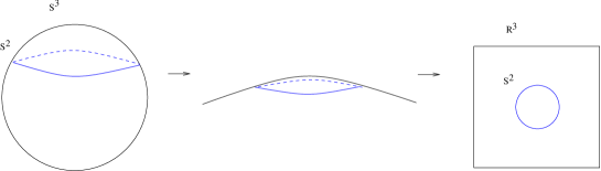
Figure 14: The limit turning a conjugacy class into an orbit for the example of $G=SU(2)$. We keep the size of the conjugacy class (orbit) fixed, while rescaling the group metric until it becomes flat.

The open string oscillations decouple in this limit, leaving us with a finite algebra of vertex operators corresponding to a rigid open string [16].

Appendix B Berezin quantization, coherent states and star products

The relation to Berezin quantization

We show that the algebra of matrices and spherical functions obtained by the three-string interaction in section 5 agrees with Berezin quantization [66] of the two-sphere for $SU(2)$. This shows that the construction known as the fuzzy two-sphere [28, 31] is nothing but Berezin’s quantization of a Kähler two-manifold, discussed in terms of coherent states for instance in [67]. We believe this is perhaps known to experts (see e.g. [28, 68] for suggestions to that effect), although it has not been stressed much, nor have we been able to find the detailed map in the literature. Let us proceed to prove this equivalence.

In the following, we first work in the formalism of [67], chapters 4 and 16 (mostly), and we will assume familiarity with that reference. Our strategy is to link the Berezin quantization [67] to a quantization discussed in reference [68], which is demonstrated there to be equivalent to the fuzzy sphere. So, let’s firstly perform Berezin quantization of the sphere coset manifold $SU(2)/U(1)$ explicitly. We perform a stereographic projection and parameterize the sphere by a complex variable $z$. The measure on the manifold is

$$d\mu(z,\bar{z}) = \frac{2j+1}{\pi}(1+z\bar{z})^{-2j-2}dzd\bar{z}$$ (123)

Let’s consider polynomial holomorphic functions of degree strictly less than or equal to the positive integer $2j$, with the scalar product:

$$\langle f,g\rangle = \int_{\mathbb{C}}f(\bar{z})g(z)d\mu(z,\bar{z})$$ (124)

One checks that the functions

$$f_{n}(z)=\langle z|j,n\rangle=\sqrt{\frac{(2j)!}{n!(2j-n)!}}z^{n}$$ (125)

for $n=0,1,\dots,2j$ form an orthonormal basis of the Hilbert space of dimension $2j+1$. They are in one-to-one correspondance with the basis vectors $|j,n\rangle$ which satisfy:

$$\langle j,n|j,n^{\prime}\rangle=\langle f_{n},f_{n^{\prime}}\rangle = \delta_{n,n^{\prime}}$$

$$\sum_{n=0}^{2j}|j,n\rangle\langle j,n| = 1$$ (126)

We define the coherent states:

$$|\zeta\rangle=\sum_{n=0}^{2j}f_{n}(\zeta)(1+\zeta\bar{\zeta})^{-j}|j,n\rangle$$ (127)

where $\zeta\in\mathbb{C}$. They satisfy:

$$\int_{\mathbb{C}}|\zeta\rangle\langle\zeta|(1+\zeta\bar{\zeta})^{2j}d\mu(\zeta,\bar{\zeta})=1$$ (128)

where the measure is the one given in $(\ref{zmeasure})$. Note that:

$$\int_{\mathbb{C}}|z\rangle\langle z|d\mu(z,\bar{z})=1$$ (129)

We also define the kernel $L$:

$$L(\zeta,z) = \sum_{n=0}^{2j}f_{n}(z)f_{n}(\zeta)=(1+z\zeta)^{2j}$$

$$\langle z|\zeta\rangle = L(z,\zeta)(1+\zeta\bar{\zeta})^{-j}$$ (130)

Using this kernel, it is possible to go from the $|z\rangle$ basis to the $|\zeta\rangle$ basis and vice-versa (though both $z$ and $\zeta$ are complex numbers, one should not confuse the associated basis vectors that are different). For instance, $\langle\zeta|j,n\rangle(1+\zeta\bar{\zeta})^{j}=f(\bar{\zeta})$. From the formula for the kernel, we easily compute the norm:

$$\langle\zeta^{\prime}|\zeta\rangle=L(\zeta,\bar{\zeta}^{\prime})(1+\zeta\bar{\zeta})^{-2j}$$ (131)

e.g. $\langle\zeta|\zeta\rangle=1$. Defining a symbol associated to an operator $F$ in the Hilbert space, following Berezin:

$$F(z,\bar{z}) = \frac{\langle\bar{z}|F|\bar{z}\rangle}{\langle\bar{z}|\bar{z}\rangle}$$ (132)

we can compute the symbol associated to the product of operators:

$$F_{1.2}(z,\bar{z}) = \frac{\langle\bar{z}|F_{1}F_{2}|\bar{z}\rangle}{\langle\bar{z}|\bar{z}\rangle}$$

$$= \int_{\mathbb{C}}\langle\bar{z}|F_{1}|\bar{\zeta}\rangle\langle\bar{\zeta}|F_{2}|\bar{z}\rangle\ \frac{(1+\zeta\bar{\zeta})^{2j}}{\langle\bar{z}|\bar{z}\rangle}d\mu(\zeta,\bar{\zeta})$$

$$= \int_{\mathbb{C}}F_{1}(z,\bar{\zeta})F_{2}(\zeta,\bar{z})\frac{\langle\bar{z}|\bar{\zeta}\rangle\langle\bar{\zeta}|\bar{z}\rangle}{\langle\bar{z}|\bar{z}\rangle}(1+\zeta\bar{\zeta})^{2j}d\mu(\zeta,\bar{\zeta})$$

$$= \int_{\mathbb{C}}F_{1}(z,\bar{\zeta})F_{2}(\zeta,\bar{z})\left(\frac{(1+z\zeta)(1+\bar{z}\bar{\zeta})}{(1+z\bar{z})}\right)^{2j}d\mu(\zeta,\bar{\zeta})$$

At this point, note that this definition of the product of symbols (i.e. functions) associated to the product of (bounded) operators in a given finite dimensional Hilbert space is the same as the definition adopted by the authors of reference [68] (see their formula (8)). Thus, the product studied in [68] is the product of symbols in Berezin quantization, within the formalism of coherent states. This is our first main point.

For comparison with various references in the literature, it can be useful to express the product differently, using a particular fixed spin $j$ unitary irreducible representation of the group $SU(2)$, $T(g)$. Using this representation, we can express operators $F$ in terms of functions $\tilde{f}$ on the group via the relation:

$$F = \int dg\langle\bar{z}|T(g)|\bar{z}\rangle\tilde{f}(g)$$ (134)

We can then express the product of the corresponding symbols in terms of the (tilded) functions, if we so desire.

Also, given the representation $T(g)$ of the group, we can associate to it a kernel function $\omega(g,\bar{z})=\langle\bar{z}|T(g)|\bar{z}\rangle/\langle\bar{z}|\bar{z}\rangle$ which is the symbol of $T(g)$, for each $g$. The symbol $F(z,\bar{z})$ of an operator $F$ is then the transform of the function $\tilde{f}$ using the kernel function $\omega$.

The operator $T(g)$ acts as follows:

$$\langle z|T(g)|j,n\rangle = T(g)f_{n}(z)=(\beta z+\bar{\alpha})^{2j}f_{n}\left(\frac{\alpha z-\bar{\beta}}{\beta z+\bar{\alpha}}\right)$$ (135)

We can then compute the symbol of the operator $T(g)$:

$$\frac{\langle\bar{z}|T(g)|\bar{z}\rangle}{\langle\bar{z}|\bar{z}\rangle} = (1+z\bar{z})^{-2j}\sum_{n=0}^{2j}\langle\bar{z}|T(g)|j,n\rangle\langle j,n|\bar{z}\rangle$$ (136)

$$= (1+z\bar{z})^{-2j}(\bar{\alpha}+\beta\bar{z}-\bar{\beta}z+\alpha z\bar{z})^{2j}$$

This indeed agrees with the kernel (46) in [68].

More crucial for comparison with previous sections is the subalgebra of star polynomials identified in [68]. We define a set of symbols which are obtained by acting with the left-invariant derivative on the symbol of $T(g)$ at the identity:

$$\phi_{j}(\bar{z}) = \imath(X_{j}\omega(e,\bar{z}))$$ (137)

The operator associated to this symbol is thus $(X_{j}T)(e)$.

It should be noted that these operators are, from the perspective of the group $G$, nothing but the generators of the representation $T(g)$. Thus, the product naturally satisfies the Lie algebra relations (see [68]). Since these are constant $(2j+1)\times(2j+1)$ matrices, they naturally form a (small) subalgebra of the algebra of symbols. It is clear (via the definition in terms of matrices) that the star product closes within this space of symbols. It is this subalgebra that can be identified as the fuzzy sphere [68]. Thus, the fuzzy sphere coincides with the (subalgebra of the symbols appearing in the) Berezin quantization of the two-sphere.

Algebraic limits

Now that we established that the fuzzy sphere is the Berezin quantization of the sphere, we can use the mathematical studies of Berezin quantization to define classical limits of the fuzzy sphere product. The sense in which the limiting procedure from the Berezin quantization of the manifold to the classical manifold is well-behaved has been the subject of many investigations. A mathematically precise treatment is in [69] and is based on a quantum Gromov-Hausdorff distance defined for $C^{\ast}$ algebras which is based on the limits defined in [70, 71]. A good physical understanding for these limits follows from the work of [72, 73], where the classical free energy (or other observables) are recovered as the large dimension limit of a quantum spin system, by proving two inequalities for the free energy (or other observables), thus sandwiching a classical observable in the semi-classical $h\to 0$ limit. We refer to [69] for a recent discussion of these limits and further developments. We conclude that the classical limit of the Berezin sphere is well-behaved in this sense.

The relation to star products

In this section, we want to investigate the link of our construction of associative products to deformation quantization. Note that in Berezin quantization it is proved that the associative product of functions consists of a first term that is the ordinary product, a second term that is the deformation in the direction of the Poisson structure, and so on (see e.g. [67]). Thus, it is natural to think of the function algebra appearing after Berezin quantization as a deformation of the ordinary function algebra on the two-sphere. Here, we want to recall rigorous mathematical results that connect Berezin quantization to geometric quantization and deformation quantization.

We first recall from [74] that the space of Berezin symbols includes the space of quantizable functions in geometric quantization. For a compact manifold, we recall that the space of symbols is a finite dimensional subspace of the space of smooth functions on the manifold $M$. In fact, in the case of the sphere, it exactly coincides with the algebra of Lie algebra generators evaluated in the coherent state basis. It is moreover shown in [74] quite generally, that the Berezin quantization of a space using a line bundle $L$ to the power $N$ is contained in the quantization of the space with line bundle $L^{N+1}$. For the sphere, this is simply the statement that the algebra of generators for the $N$ dimensional representation is included in the algebra of generators for the $N+1$ dimensional representation.

Crucially, the paper [74] shows that in the large $N$ limit, the algebra of symbols, which is the union of the algebra of symbols at any $N$ is dense in the subalgebra of continuous functions on $M$. In particular, the algebra separates any two points in $M$.

Furthermore, the product of symbols of operators can be interpreted, for any given $N$ as an associative product of functions on the manifold $M$ – we call this product the $N$-product. In a follow-up paper [75] it is shown that there is a formal differential star product with deformation parameter $\nu=i/(4\pi N)$ which coincides with the asymptotic expansion of the $N$-product for any compact generalized flag manifold. The differential operators arising in the expansion depend only on the geometry of the manifold $M$, and the remainder term goes to zero like a power of $N$ (where the power depends on the number of terms in the expansion). Moreover, for any hermitian symmetric space, the formal star product is convergent.

Thus, the results of [74, 75] show in a precise way that the star $N$-product arising from Berezin quantization of the two-sphere (amongst other manifolds) asymptotes to a formal $*$-product on the two-sphere in the large $N$ limit. (This completes a proof sketched in [25].) We must note here that the star product so obtained is formal. The formal series defining the multiplication of functions does not have a fixed radius of convergence for a set of functions which is dense in the set of continuous functions on the sphere.

Appendix C The ${}_{3}F_{2}(1)$ hypergeometric functions and 3j symbol transformations

In this appendix we will recall relations between ${}_{3}F_{2}(1)$ hypergeometric functions [76, 77, 78, 79] and use these relations to show how one can determine the symmetry properties of $SU(2)$ or $SU(1,1)$ 3j symbols.

Whipple functions

We first introduce Whipple’s notation, which is a very compact way to write down the various transformations relating different ${}_{3}F_{2}(1)$ functions. In this notation, one has six complex parameters $r_{i}$, $i=0,1,...,5$, which obey the following condition:

$$r_{0}+r_{1}+r_{2}+r_{3}+r_{4}+r_{5}=0$$ (138)

therefore leaving us with five degrees of freedom. One then defines the following variables:

$$\alpha_{lmn} = \frac{1}{2}+r_{l}+r_{m}+r_{n}$$

$$\beta_{lm} = 1+r_{l}-r_{m}$$ (139)

Some simple remarks are in order: $\alpha_{lmn}$ is completely symmetric, while $\beta_{lm}=2-\beta_{ml}$. Also, note that due to equation $(\ref{sumr})$, we have $\alpha_{lmn}=1-\alpha_{ijk}$ where the indices $i,j,k$ are all different from $l,m,n$.

Using this notation, the (Thomae-)Whipple functions are:

$$F_{p}(l;m,n) = \frac{1}{\Gamma(\alpha_{ghj},\beta_{ml},\beta_{nl})}\ {{}_{3}}F_{2}\left(\begin{array}[]{c}\alpha_{gmn},\ \alpha_{hmn},\ \alpha_{jmn}\\ \beta_{ml}\ ,\ \ \beta_{nl}\end{array};1\right)$$ (142)

$$F_{n}(l;m,n) = \frac{1}{\Gamma(\alpha_{lmn},\beta_{lm},\beta_{ln})}\ {{}_{3}}F_{2}\left(\begin{array}[]{c}\alpha_{lgh},\ \alpha_{lgj},\ \alpha_{lhj}\\ \beta_{lm}\ ,\ \ \beta_{ln}\end{array};1\right)$$ (145)

where $g$, $h$ and $j$ are indices all different from $l$, $m$ and $n$. Note that any $F_{n}(l;m,n)$ function is obtained from the corresponding $F_{p}(l;m,n)$ function by changing the signs of all the parameters $r_{i}$. The function $F_{p}(l;m,n)$ is well-defined if $\Re\alpha_{ghj}>0$ and $F_{n}(l;m,n)$ is well-defined if $\Re\alpha_{lmn}>0$. This is related to the fact that the defining series for ${}_{3}F_{2}(a_{1},a_{2},a_{3};b_{1},b_{2};1)$ is well-defined iff $s=b_{1}+b_{2}-a_{1}-a_{2}-a_{3}$ is such that $\Re s>0$, assuming that no argument is a negative integer. Things are a little different if at least one $a_{i}$ is a negative integer, since in this case ${}_{3}F_{2}(a_{1},a_{2},a_{3};b_{1},b_{2};1)$ can be expressed as a finite sum and there is no more requirement on s. There is however a complication if some $a_{i}$’s and some $b_{j}$’s are negative integers at the same time, for in this case there is no clear limiting procedure that would allow us to define ${}_{3}F_{2}(1)$. Assuming that $a_{i_{0}}=-N$ is the largest of all negative integers $a_{i}$ and that any $b_{j}$ that is a negative integer is smaller than $-N$, a reasonable definition is:

$${}_{3}F_{2}\left(\begin{array}[]{ccc}a_{1},&a_{2},&a_{3}\\ b_{1},&b_{2}&\end{array}\ ;1\right)=\sum_{n=0}^{N}\ \frac{(a_{1})_{n}(a_{2})_{n}(a_{3})_{n}}{(b_{1})_{n}(b_{2})_{n}}\ \frac{1}{n!}$$ (148)

i.e we have truncated the infinite sum. We have used the Pochammer symbol $(a)_{n}=\frac{\Gamma(a+n)}{\Gamma(a)}$.

Two-term and three-term relations

Relations between ${}_{3}F_{2}(1)$ functions are standard and can be elegantly written in Whipple’s notation. There are two kinds of such relations. The first one consists of two-term relations:

$$F_{p}(l;m,n) = F_{p}(l;m^{\prime},n^{\prime})$$

$$F_{n}(l;m,n) = F_{n}(l;m^{\prime},n^{\prime})$$ (149)

i.e they are simply equivalent to the statement that both $F_{p}(l;m,n)$ and $F_{n}(l;m,n)$ actually do not depend on $m$ and $n$ (therefore we will denote them by $F_{p}(l)$ and $F_{n}(l)$). The second kind of relations are three-term relations:

$$\frac{\sin{\pi\beta_{23}}}{\pi\Gamma(\alpha_{023})}F_{p}(0) = \frac{F_{n}(2)}{\Gamma(\alpha_{134},\alpha_{135},\alpha_{345})}-\frac{F_{n}(3)}{\Gamma(\alpha_{124},\alpha_{125},\alpha_{245})}$$ (150)

$$\frac{\sin{\pi\beta_{32}}}{\pi\Gamma(\alpha_{145})}F_{n}(0) = \frac{F_{p}(2)}{\Gamma(\alpha_{012},\alpha_{024},\alpha_{025})}-\frac{F_{p}(3)}{\Gamma(\alpha_{013},\alpha_{034},\alpha_{035})}$$

$$\frac{\sin{\pi\beta_{45}}\ F_{p}(0)}{\Gamma(\alpha_{012},\alpha_{013},\alpha_{023})} = -\frac{\sin{\pi\beta_{50}}\ F_{p}(4)}{\Gamma(\alpha_{124},\alpha_{134},\alpha_{234})}-\frac{\sin{\pi\beta_{04}}\ F_{p}(5)}{\Gamma(\alpha_{125},\alpha_{135},\alpha_{235})}$$

$$\frac{\sin{\pi\beta_{54}}\ F_{n}(0)}{\Gamma(\alpha_{145},\alpha_{245},\alpha_{345})} = -\frac{\sin{\pi\beta_{05}}\ F_{n}(4)}{\Gamma(\alpha_{015},\alpha_{025},\alpha_{035})}-\frac{\sin{\pi\beta_{40}}\ F_{n}(5)}{\Gamma(\alpha_{014},\alpha_{024},\alpha_{034})}$$

$$\frac{F_{p}(0)}{\Gamma(\alpha_{012},\alpha_{013},\alpha_{023},\alpha_{014},\alpha_{024},\alpha_{034})} = K_{0}F_{p}(5)-\frac{\sin{\beta_{05}}\ F_{n}(0)}{\Gamma(\alpha_{123},\alpha_{124},\alpha_{134},\alpha_{234})}$$

$$\frac{F_{n}(0)}{\Gamma(\alpha_{125},\alpha_{135},\alpha_{235},\alpha_{145},\alpha_{245},\alpha_{345})} = K_{0}F_{n}(5)-\frac{\sin{\beta_{50}}\ F_{p}(0)}{\Gamma(\alpha_{015},\alpha_{025},\alpha_{035},\alpha_{045})}$$

where $K_{0}=\frac{1}{\pi^{3}}\left(\sin{\pi\alpha_{145}}\sin{\pi\alpha_{245}}\sin{\pi\alpha_{345}}+\sin{\pi\alpha_{123}}\sin{\pi\beta_{40}}\sin{\pi\beta_{50}}\right)$. These six identities, up to permutation of indices, give us 120 independent relations between ${}_{3}F_{2}(1)$ functions. These three-term relations may reduce to two-term relations when one or more $\alpha_{lmn}$ is a negative integer, as we will see below.

An integer limit of Whipple’s relations

Let us proceed to find Whipple’s relations in the specific case that is needed in order to understand transformations of the 3j symbols, whether we consider $SU(2)$ or $SU(1,1)$. In these cases the arguments of the hypergeometric functions used in the expressions of the 3j symbols are all integer. Since Whipple’s relations are valid in the generic case of complex parameters, relations in the case of integer parameters should be obtained from a limiting procedure. With no loss of generality, we are free to choose:

$$\alpha_{145} = -n+\epsilon\ ,\hskip 34.14322pt\alpha_{014}=-n_{2}+\epsilon_{2}$$

$$\alpha_{245} = -n^{\prime}_{1}+\epsilon^{\prime}_{1}\ ,\hskip 28.45274pt\alpha_{015}=-n^{\prime}_{2}+\epsilon^{\prime}_{2}$$ (151)

$$\alpha_{345} = -n_{1}+\epsilon_{1}$$

where $\epsilon,\epsilon_{1},\epsilon^{\prime}_{1},\epsilon_{2},\epsilon^{\prime}_{2}$ are real and tend to zero. The behavior of all other parameters $\alpha_{lmn}$, $\beta_{lm}$ is then fixed.

One important remark is that, though the $\epsilon$’s may be anything a priori, the limiting procedure must satisfy some consistency conditions. To be more precise, the fact that all 3j symbols are real and that all ratios of 3j symbols, for $SU(2)$ on one hand, and for $SU(1,1)$ on the other hand, are of modulus one implies that:

$$|\epsilon|=|\epsilon_{1}|=|\epsilon^{\prime}_{1}|=|\epsilon_{2}|=|\epsilon^{\prime}_{2}|$$ (152)

and that the relative signs between $\epsilon$’s must also be of the following kind only (up to a global sign that we use to fix $\epsilon>0$):

$$\begin{array}[]{ccccc}\epsilon&\epsilon_{1}&\epsilon^{\prime}_{1}&\epsilon_{2}&\epsilon^{\prime}_{2}\\ +&+&+&+&-\\ +&+&+&-&+\\ +&+&-&+&+\\ +&-&+&+&+\\ +&+&+&-&-\\ +&-&-&+&+\end{array}$$ (160)

Now that we know what kind of limit we can consider, and that results should not depend on which of the six possible limits we take, it is possible to find the following relations resulting from equations $(\ref{3Fpn})$ in this limit:

$$F_{p}(0) = (-1)^{\beta_{04}-1}\Gamma\left(\begin{array}[]{ccc}\alpha_{012}&\alpha_{013}&\alpha_{023}\\ \alpha_{124}&\alpha_{134}&\alpha_{234}\end{array}\right)F_{p}(4)$$ (163)

$$= (-1)^{\beta_{05}-1}\Gamma\left(\begin{array}[]{ccc}\alpha_{012}&\alpha_{013}&\alpha_{023}\\ \alpha_{125}&\alpha_{135}&\alpha_{235}\end{array}\right)F_{p}(5)$$ (166)

$$F_{n}(1) = (-1)^{\beta_{12}-1}\Gamma\left(\begin{array}[]{ccc}\alpha_{023}&\alpha_{234}&\alpha_{235}\\ \alpha_{013}&\alpha_{134}&\alpha_{135}\end{array}\right)F_{n}(2)$$ (169)

$$= (-1)^{\beta_{13}-1}\Gamma\left(\begin{array}[]{ccc}\alpha_{023}&\alpha_{234}&\alpha_{235}\\ \alpha_{012}&\alpha_{124}&\alpha_{125}\end{array}\right)F_{n}(3)$$ (172)

$$F_{p}(2) = -\Gamma\left(\begin{array}[]{ccc}\alpha_{023}&\alpha_{234}&\alpha_{235}\\ \alpha_{013}&\alpha_{125}&\alpha_{135}\end{array}\right)F_{p}(1)$$ (175)

$$= -\Gamma\left(\begin{array}[]{ccc}\alpha_{012}&\alpha_{124}&\alpha_{125}\\ \alpha_{013}&\alpha_{134}&\alpha_{135}\end{array}\right)F_{p}(3)$$ (178)

$$F_{n}(4) = \Gamma\left(\begin{array}[]{ccc}\alpha_{012}&\alpha_{013}&\alpha_{023}\\ \alpha_{124}&\alpha_{134}&\alpha_{234}\end{array}\right)F_{n}(0)$$ (181)

$$= \Gamma\left(\begin{array}[]{ccc}\alpha_{125}&\alpha_{135}&\alpha_{235}\\ \alpha_{124}&\alpha_{134}&\alpha_{234}\end{array}\right)F_{n}(5)$$ (184)

$$F_{p}(0) = (-1)^{\alpha_{145}}\Gamma\left(\begin{array}[]{cc}\alpha_{012}&\alpha_{013}\\ \alpha_{234}&\alpha_{235}\end{array}\right)F_{n}(1)$$ (187)

$$\epsilon^{2}F_{p}(0) \sim (-1)^{\beta_{45}-1}\frac{\Gamma(\alpha_{013})}{\Gamma(\alpha_{123},\alpha_{124},\alpha_{125},\alpha_{234},\alpha_{235})}\ F_{p}(2)$$

$$\epsilon^{2}F_{n}(1) \sim (-1)^{\beta_{23}}\frac{\Gamma(\alpha_{234})}{\Gamma(\alpha_{012},\alpha_{013},\alpha_{123},\alpha_{125},\alpha_{135})}\ F_{n}(4)$$

Note that, while some Whipple functions are finite, like $F_{p}(0)$, others tend to zero in the integer limit.

From the above relations it is possible to find the symmetry relations of 3j symbols, by choosing appropriately the parameters $\alpha_{lmn}$, $\beta_{lm}$. There is however one subtlety that arises in some cases: $\Gamma$ function prefactors may contribute to the overall sign that relate any 3j symbol to any other 3j symbol. Recall for instance the expression of the $SU(1,1)$ 3j symbol that was given in equation $(\ref{3jsu11})$. It is not clear whether one should put a given $\Gamma$ function (say $\Gamma(m_{1}+j_{1})$ for instance) inside or outside the square root, since this does not matter for the $+++$ 3j symbol. It would however matter if one would try to compute some other 3j symbol, like $---$.

This last subtlety can be solved by computing explicitly a 3j symbol for $SU(1,1)$ involving at least one $\mathcal{D}^{-}$ representation. This can be done using a result from [35]. The 3j symbol given in [35] is related to our formula $(\ref{3jsu11})$ by:

$$\left[\begin{array}[]{ccc}j_{1}&j_{2}&j\\ m_{1}&m_{2}&-m\end{array}\right]^{+++}_{D.}=(-1)^{j+j_{1}-m_{2}+1}\left[\begin{array}[]{ccc}j_{2}&j_{1}&j\\ m_{2}&m_{1}&-m\end{array}\right]^{+++}_{us}$$ (192)

$$=(-1)^{j_{1}-m_{1}}\sqrt{\frac{(m_{1}+j_{1}-1)!(m_{1}-j_{1})!(m_{2}+j_{2}-1)!(m_{2}-j_{2})!}{(m-j)!(m+j-1)!}}$$

$$\times\sqrt{(j+j_{1}+j_{2}-2)!(j+j_{1}-j_{2}-1)!(j-j_{1}+j_{2}-1)!(j-j_{1}-j_{2})!}$$

$$\times\frac{1}{(m_{1}+j_{1}-1)!(m_{1}-j_{1})!}\cdot\frac{1}{(j+j_{2}-m_{1}-1)!(j-j_{2}-m_{1})!}$$

$$\times\ _{3}F_{2}\left(\begin{array}[]{c}j-m,\ \ 1-m_{1}-j_{1},\ \ j_{1}-m_{1}\\ j+j_{2}-m_{1},\ \ j-j_{2}-m_{1}+1\end{array};1\right)$$ (195)

It satisfies:

$$\left[\begin{array}[]{ccc}j_{1}&j_{2}&j\\ m_{1}&m_{2}&-m\end{array}\right]^{+++}_{D.} = (-1)^{j-j_{1}-j_{2}}\left[\begin{array}[]{ccc}j_{2}&j_{1}&j\\ m_{2}&m_{1}&-m\end{array}\right]^{+++}_{D.}$$ (200)

$$= \left[\begin{array}[]{ccc}j_{1}&j_{2}&j\\ -m_{1}&-m_{2}&m\end{array}\right]^{+++}_{D.}$$ (203)

This calculation forces us to place particular $\Gamma$ functions (factorials) outside of the square root according to the above formula for the 3j symbols. This resolves the ambiguity in the relative sign of the 3j symbols as we analytically continue. Other symmetry relations of the $SU(1,1)$ 3j symbols follow directly from equations $(\ref{integerlimitw})$.

References

- [1] N. Seiberg and E. Witten, JHEP 9909 (1999) 032 [arXiv:hep-th/9908142].
- [2] M. R. Douglas and N. A. Nekrasov, Rev. Mod. Phys. 73 (2001) 977 [arXiv:hep-th/0106048].
- [3] H. S. Snyder, Phys. Rev. 71 (1947) 38.
- [4] V. Schomerus, JHEP 9906 (1999) 030 [arXiv:hep-th/9903205].
- [5] G. W. Moore and N. Seiberg, Commun. Math. Phys. 123 (1989) 177.
- [6] J. L. Cardy and D. C. Lewellen, Phys. Lett. B 259, 274 (1991).
- [7] H. B. Nielsen and D. Rohrlich, Nucl. Phys. B 299 (1988) 471.
- [8] A. Alekseev, L. D. Faddeev and S. L. Shatashvili, J. Geom. Phys. 5 (1988) 391.
- [9] A. P. Balachandran, G. Marmo, B. S. Skagerstam and A. Stern, Lect. Notes Phys. 188 (1983) 1.
- [10] A. A. Kirillov, “Elements of the theory of representations”, Springer-Verlag, Berlin-New York, 1976, and especially “Lectures on the orbit method”, Graduate studies in Mathematics, 64, AMS, Rhode Island, 2004.
- [11] J. Troost and A. Tsuchiya, JHEP 0306 (2003) 029 [arXiv:hep-th/0304211].
- [12] N. M. J. Woodhouse, “Geometric Quantization”, New York, USA: Clarendon (1992).
- [13] W. I. Taylor, arXiv:hep-th/9310040.
- [14] D. Bigatti and L. Susskind, Phys. Rev. D 62 (2000) 066004 [arXiv:hep-th/9908056].
- [15] A. Y. Alekseev and V. Schomerus, Phys. Rev. D 60 (1999) 061901 [arXiv:hep-th/9812193].
- [16] A. Y. Alekseev, A. Recknagel and V. Schomerus, JHEP 9909 (1999) 023 [arXiv:hep-th/9908040].
- [17] B. Morariu, Nucl. Phys. B 734, 156 (2006) [arXiv:hep-th/0408018].
- [18] J. McGreevy, L. Susskind and N. Toumbas, JHEP 0006 (2000) 008 [arXiv:hep-th/0003075].
- [19] E. Witten, Nucl. Phys. B 268, 253 (1986).
- [20] G. Pradisi, A. Sagnotti and Y. S. Stanev, Phys. Lett. B 381 (1996) 97 [arXiv:hep-th/9603097].
- [21] I. Runkel, Nucl. Phys. B 549, 563 (1999) [arXiv:hep-th/9811178].
- [22] R. E. Behrend, P. A. Pearce, V. B. Petkova and J. B. Zuber, Nucl. Phys. B 570 (2000) 525 [Nucl. Phys. B 579 (2000) 707] [arXiv:hep-th/9908036].
- [23] G. Felder, J. Frohlich, J. Fuchs and C. Schweigert, J. Geom. Phys. 34 (2000) 162 [arXiv:hep-th/9909030].
- [24] G. Felder, J. Frohlich, J. Fuchs and C. Schweigert, Compos. Math. 131 (2002) 189 [arXiv:hep-th/9912239].
- [25] L. Freidel and K. Krasnov, J. Math. Phys. 43, 1737 (2002) [arXiv:hep-th/0103070].
- [26] N. Vilenkin and A. Klymik, Representation of Lie groups and Special Functions, Volume 1, mathematics and its applications, Kluwer academic publisher, 1993.
- [27] E. P. Wigner., In Quantum Theory of Angular Momentum, eds. L. C. Biedenharn, H. van Dam, pp. 89-133. New York: Academic Press, 1965. (Original: 1940 (unpublished).)
- [28] J. Hoppe, Int. J. Mod. Phys. A 4, 5235 (1989).
- [29] G. D’Appollonio and E. Kiritsis, Nucl. Phys. B 674, 80 (2003) [arXiv:hep-th/0305081].
- [30] G. D’Appollonio and E. Kiritsis, Nucl. Phys. B 712 (2005) 433 [arXiv:hep-th/0410269].
- [31] J. Madore, Class. Quant. Grav. 9, 69 (1992).
- [32] N. Mukunda and B. Radhakrishnan, “Clebsch-gordan problem and coefficients for the three-dimensional lorentz J. Math. Phys. 15 (1974) 1320.
- [33] N. A. Liskova and A. N. Kirillov, Int. J. Mod. Phys. A 7S1B, 611 (1992) [arXiv:hep-th/9212064].
- [34] S. Davids, J. Math. Phys. 41 (2000) 924 [arXiv:gr-qc/9807061].
- [35] S. Davids, arXiv:gr-qc/0110114.
- [36] A. Y. Alekseev and A. Z. Malkin, Commun. Math. Phys. 162 (1994) 147 [arXiv:/9303038].
- [37] K. Gawedzki, Commun. Math. Phys. 139 (1991) 201.
- [38] F. Falcet and K. Gawedzki, arXiv:hep-th/9109023.
- [39] B. Morariu, Int. J. Mod. Phys. A 14 (1999) 919 [arXiv:physics/9710010].
- [40] M. f. Chu and P. Goddard, Phys. Lett. B 337, 285 (1994) [arXiv:hep-th/9407116].
- [41] B. Y. Hou, B. Y. Hou and Z. Q. Ma, Commun. Theor. Phys. 13, 341 (1990).
- [42] B. Y. Hou, B. Y. Hou and Z. Q. Ma, BIHEP-TH-89-7
- [43] N. Vilenkin and A. Klymik, Representation of Lie groups and Special Functions, Volume 3, mathematics and its applications, Kluwer academic publisher, 1993.
- [44] P. Podles, Lett. Math. Phys. 14, 193 (1987).
- [45] B. Jurco and P. Stovicek, Comm. Math. Phys. 152, no. 1 (1993), 97
- [46] B. Jurco and P. Stovicek, Commun.Math.Phys. 182 (1996) 221 [arxiv:hep-th/9403114].
- [47] K. Sfetsos, Phys. Rev. D 50 (1994) 2784 [arXiv:hep-th/9402031].
- [48] J. M. Figueroa-O’Farrill and S. Stanciu, Phys. Lett. B 327 (1994) 40 [arXiv:hep-th/9402035].
- [49] J. M. Maldacena and H. Ooguri, Phys. Rev. D 65 (2002) 106006 [arXiv:hep-th/0111180].
- [50] S. Ribault, JHEP 0509, 045 (2005) [arXiv:hep-th/0507114].
- [51] B. Ponsot and J. Teschner, Commun. Math. Phys. 224, 613 (2001) [arXiv:math.qa/0007097].
- [52] B. Ponsot and J. Teschner, Nucl. Phys. B 622, 309 (2002) [arXiv:hep-th/0110244].
- [53] S. Ribault and J. Teschner, JHEP 0506, 014 (2005) [arXiv:hep-th/0502048].
- [54] K. Hosomichi and S. Ribault, arXiv:hep-th/0610117.
- [55] L. Alvarez-Gaume, C. Gomez and G. Sierra, Phys. Lett. B 220 (1989) 142.
- [56] A. Y. Alekseev and I. T. Todorov, Nucl. Phys. B 421, 413 (1994) [arXiv:hep-th/9307026].
- [57] A. Weinstein, Traces and triangles in symmetric symplectic spaces, Contemp. Math. 179 (1994), Amer. Math. Soc., Providence, RI, 261-270.
- [58] A. Weinstein, Deformation theory and symplectic geometry (Ascona, 1996), 301–314, Math. Phys. Stud., 20, Kluwer Acad. Publ., Dordrecht, 1997.
- [59] M.V. Karasev Izv. Akad. Nauk SSSR Ser. Mat. 50 (1986), no. 3, 508–538, 638.
- [60] A. Coste, P. Dazord, and A. Weinstein, Groupoides symplectiques. Publications du Departement de Mathematiques. Nouvelle Serie A, Vol. 2, i–ii, 1–62, Publ. Dep. Math. Nouvelle Serie A, 87-2, Univ. Claude-Bernard, Lyon, 1987.
- [61] A.Weinstein, Symplectic geometry and mathematical physics (Aix-en-Provence, 1990), 446–461, Progr. Math., 99, Birkhauser Boston, Boston, MA, 1991.
- [62] S. Zakrzewski, Comm. Math. Phys. 134 (1990), no. 2, pp. 347.
- [63] A. Unterberger et J. Unterberger, C. R. Acad. Sci. Paris Ser. I Math. 296 (1983), no. 11, 465–468.
- [64] A. Unterberger et J. Unterberger, Ann. Sci. Ecole Norm. Sup. (4) 21 (1988), no. 1
- [65] A. Y. Alekseev, S. Fredenhagen, T. Quella and V. Schomerus, Nucl. Phys. B 646 (2002) 127 [arXiv:hep-th/0205123].
- [66] F. Berezin, Math. USSR Izvestija 8, 1109 (1974).
- [67] A. M. Perelomov, “Generalized Coherent States And Their Applications,”
- [68] H. Grosse and P. Presnajder, Lett. Math. Phys. 28, 239 (1993).
- [69] M. A. Rieffel, arXiv:math.oa/0108005.
- [70] N. P. Landsman, J. Math. Phys. 39, 6372 (1998).
- [71] M. Bordemann, E. Meinrenken and M. Schlichenmaier, Commun. Math. Phys. 165, 281 (1994) [arXiv:hep-th/9309134].
- [72] E. H. Lieb, Commun. Math. Phys. 31 (1973) 327.
- [73] B. Simon, Commun. Math. Phys. 71 (1980) 247.
- [74] J. Rawnsley, M. Cahen and S. Gutt, J. Geom. Phys. 7, 45 (1990).
- [75] J. Rawnsley, M. Cahen and S. Gutt, “Quantization Of Kaehler Manifolds. II
- [76] Whipple, F. J. W. ”Well-Poised Series and Other Generalized Hypergeometric Series.” Proc. London Math. Soc. Ser. 2 25, 525-544, 1926.
- [77] Whipple, F. J. W. ”On Well-Poised Series, Generalized Hypergeometric Series Having Parameters in Pairs, Each Pair with the Same Sum.” Proc. London Math. Soc. 24, 247-263, 1926.
- [78] Whipple, F. J. W. ”A Fundamental Relation Between Generalized Hypergeometric Series.” Proc. London Math. Soc. 26, 257-272, 1927.
- [79] Lucy Joan Slater. Generalized Hypergeometric Functions. Cambridge University Press, 1966.