CERN-PH-TH/2006-218
LMU-ASC 66/06
MPP-2006-135

This review article provides a pedagogical introduction into various classes of chiral string compactifications to four dimensions with D-branes and fluxes. The main concern is to provide all necessary technical tools to explicitly construct four-dimensional orientifold vacua, with the final aim to come as close as possible to the supersymmetric Standard Model. Furthermore, we outline the available methods to derive the resulting four-dimensional effective action. Finally, we summarize recent attempts to address the string vacuum problem via the statistical approach to D-brane models.

Pacs numbers: 11.25.Mj, 11.25.-w, 11.25.Wx

  e-mail address of the review: revibw@mppmu.mpg.de

1 INTRODUCTION

The history of theoretical particle physics has been extremely successful. Based on the principles of quantum mechanics and its relativistic generalization in the form of quantum field theory a unified framework could be developed over the second half of the twentieth century allowing the prediction of many experimental data with amazing precision. In the so-called electro-weak Standard Model (SM) of particle physics the fundamental particles, the quarks, leptons and the Higgs scalar, interact via three types of gauge interactions, namely the strong, the weak and the electromagnetic interaction. The fermionic matter particles come in three identical copies which only differ by their mass. The third family is hierarchically heavier than the first two. All stable particles we observe in our universe consist only of fermions from the first and lightest family. The only ingredient of the SM not yet detected experimentally is the Higgs particle, a scalar boson that triggers spontaneous gauge symmetry breaking at the electro-weak scale by a vacuum expectation value and gives masses to the gauge bosons of the weak interactions as well as to all the matter fields.

Given the fact that the SM is very powerful in explaining a surprisingly large number of independent experimental data, one may still feel not quite satisfied with a purely phenomenological approach. From a more conceptual point of view we do not know the principles which fix the numerical parameters that define the Lagrangian of the SM to the values they have in our universe. In the SM Lagrangian they appear simply as free parameters like coupling constants and mixing angles which we fix a posteriori by observation. Is it possible to actually calculate their values at some higher scale from a more fundamental theory? Moreover, the choice we make when we single out the field theory to describe particle interactions involves an even larger degree of arbitrariness. The $SU(3)\times SU(2)\times U(1)_{Y}$ gauge invariant and renormalizable Lagrangian with the given matter spectrum of quarks and leptons in three generations is just one specific model out of the infinite class of possible local quantum field theories. Beyond these issues of arbitrary choices there is also the question of naturalness. On a technical level, it refers to the necessity of fine-tuning tree-level parameters to accommodate for experimentally acceptable values given the size of the perturbative quantum corrections. This reasoning has motivated most of the explicit models for extensions of the SM.

Any truly fundamental theory should somehow be able to incorporate quantum gravity at very high energies. But despite all the successes of the SM it does not seem to be a good candidate for a complete theory of elementary particle physics simply because gravity does not appear to fit into the framework of perturbative local quantum field theories in any obvious way. Trying to quantize Einstein’s theory of general relativity perturbatively around a flat background one encounters infinities in the resulting Feynman diagrams, that cannot be cured by the usual renormalization procedure.

Adding up the evidence, the SM together with classical general relativity appears to be an excellent field theory to describe our universe up to the electro-weak energy scale of $100$GeV. In a way, it works much better than we may have expected and until to date has needed only very minor modifications to explain all the low energy data. On the other hand, the SM is unsatisfactory from the perspective of searching for a fundamental theory. So we expect new physics, i.e. new particles, new interactions, or other new effects, at energies only little beyond the $100$GeV threshold, at most two orders of magnitude above it. The SM is thus expected to be only an effective theory.

The motivation for this expectation does not only follow from the theoretical reasoning but also from recent cosmological observations. From the analysis of supernovae at large red shifts and the recent precision measurement of the temperature fluctuations in the cosmic microwave background radiation, a cosmological standard scenario has been derived. It implies that roughly $70\%$ of the current energy density in the universe consists in a form of dark energy that basically behaves like a cosmological constant ${\Lambda}$, and that $26\%$ come in the form of an unknown kind of dark matter. The rest is accounted for by ordinary particles, i.e. mostly baryons. The most appealing version of this model is then known as ${\Lambda}$CDM, the cosmological constant ${\Lambda}$ together with cold dark matter. There is no straightforward realization of such a scenario within the SM, in particular due to the lack of a candidate particle species to serve as cold dark matter. Beyond that, there are various other problems which do not find good answers within the SM, such the issue of baryogenesis which requires a strong first order phase transition not found in the SM.

Another widely accepted, but still more speculative ingredient of the standard cosmology is the paradigm of inflation. It says that in a rather early period of its evolution our universe has undergone a phase of accelerated expansion. In the simplest scenarios this could have been triggered by the vacuum energy of an unidentified scalar field, the so-called inflaton. The only scalar that exists in the SM is the Higgs scalar, and it does not seem to be a reasonable inflaton candidate. All this shows that there must be physics beyond the SM.

One candidate for the new physics at the TeV scale, mainly motivated by the naturalness problem of the SM, is a supersymmetric quantum field theory that includes the SM particles as a subset. In its simplest form it assumes for each known elementary particle the existence of a superpartner with the opposite spin-statistics, i.e. the fermionic quarks and leptons have bosonic scalar partners called squarks and sleptons (s for scalar), and the gauge bosons have fermionic partners, the gauginos. The Higgs scalar would come with a fermionic partner as well, a higgsino. This model is called the minimal supersymmetric extension of the SM, the MSSM. One of its solid prediction is that the mass of the lightest neutral Higgs scalar should be around the weak scale, at least not heavier than, say, $150$GeV. Supersymmetric field theories provide a potential candidate particle species to serve as dark matter, namely the lightest supersymmetric particle (LSP). Assuming a plausible discrete symmetry called R-parity this particle is absolutely stable. Within the MSSM a very attractive concrete possibility for the LSP is the lightest neutral fermion among the superpartners, the lightest neutralino, which could produce just the right amount of cold dark matter, given favorable choices of parameters.

Since we do not observe the superpartners directly, supersymmetry has to be broken at low energies. In order not to spoil the original motivation, the breaking has to be “soft”. One option to achieve this is to start from an extended model with more fields in a so-called hidden sector which then undergoes spontaneous supersymmetry breaking. Integrating out the extra fields leads to soft breaking in the visible sector, ideally the MSSM. An example is the minimal supergravity model (mSUGRA) with spontaneous supersymmetry breaking at an intermediate scale $10^{11}-10^{13}$GeV which is communicated to the MSSM by gravitational interactions only, leading to an effective breaking scale just around a TeV. To parameterize the Lagrangian of the MSSM including these effects one has to add all the soft breaking terms to the supersymmetric theory. This entire procedure introduces many new parameters into the model, partly due to the supersymmetrization, partly due to the breaking of supersymmetry. Eventually, they would need to be determined by experiments, a formidable task beyond any present plans for future experiments. However, if supersymmetry in form of the MSSM is realized at all will be tested at the large hadron collider (LHC).

Eventually, it might turn out that a supersymmetric generalization of the SM, which is still a local quantum field theory, indeed pushes our understanding of elementary particle physics many orders of magnitude higher in energy, maybe even not far from to the Planck scale of about $10^{19}$GeV where quantum effects of gravity become important. But it does not solve any of the fundamental problems related to the shortcomings of quantum field theories, in particular supersymmetric extensions of gravity, supergravity theories, do not appear to be perturbatively renormalizable either. This may be related to the extremely small value of the cosmological constant whose unnaturalness is not cured by supersymmetry in the broken phase. In order to make progress in the direction of reconciling quantum field theory with quantum gravity one has to give up one of the implicit underlying assumptions. To take into account that space-time itself is expected to fluctuate and deviate from the classical picture of smooth geometry at the Planck scale, one can contemplate various approaches. For example, one may want to change the smoothness of the space-time itself at small Planckian distance scales and discretize in some manner. One might hope that for instance concepts like non-commutative geometry, which assumes that the space-time coordinates do not commute and instead obey an uncertainty principle, lead to a description of quantum gravity. Whether such a formulation exist is not clear at the moment, though interesting first results have been obtained. Similarly, the approach of loop quantum gravity leads to a quantization of space-time at very small distances which may or may not lead to a consistent theory of quantum gravity.

String theory starts from a rather different point of view. It postulates that the fundamental objects in nature are not point-particles but one-dimensional strings, at least this is the perturbative definition of the theory. Space-time itself together with the fields of general relativity and quantum field theories are emergent phenomena that arise as effective descriptions of string dynamics. Fundamental strings are of finite length $\ell_{s}$ and thus cannot resolve distances smaller than $\ell_{s}$, the string scale. Below this scale, there is no meaning to the geometry of space-time in perturbative string theory. String perturbation theory in fact means a quantum theory of small fluctuations of elementary strings around a given background. At larger distances such a theory is again described by an effective field theory, a quantum field theory plus general relativity and potentially with supersymmetry built in. A priori, these are the ingredients needed for a unified theory of all forces and particles.

After its discovery thirty years ago, it became clear that this at first sight quite ad hoc construction leads to many interesting consequences. By quantizing the fundamental string moving in a flat Minkowski space the first proponents of string theory realized that strings live in more than four space-time dimensions and that the space-time only becomes stable in the presence of supersymmetry. More specifically, closed strings incorporate gravity and open strings potentially non-abelian gauge interactions. For supersymmetric strings the critical space-time dimension turned out $D=10$. Moreover, the perturbative expansion of superstring theory was argued to be finite, which was shown explicitly up to two-loop order. Nowadays superstring theory is considered to be a very promising, if not the most successful, candidate for the fundamental unified theory underlying particle physics and gravity, the theory of everything. Indeed, it is very encouraging that such a simple idea in principle automatically incorporates all the features we know of that a fundamental theory must have, such as local reparametrization invariance and non-abelian gauge symmetry, plus some other ingredients which are maybe not equally essential, but which we still like, for instance supersymmetry and extra dimensions.

Around 1995 it was realized that string theory is more complex and more general than anticipated before. It not only contains strings as fundamental degrees of freedom, but also higher-dimensional objects called $p$-branes [1] (see [2, 3] for reviews). These are not present in the perturbative spectrum, since their masses scale inversely with the coupling constant. They are only relevant in the non-perturbative regime. Moreover, supersymmetry was used to argue for certain duality relations between different string theories and different string backgrounds, essentially claiming that these are only apparently different descriptions of identical physics. Everything eventually pointed towards a yet unknown theory that unifies all known string theories, called M-theory, with an eleven-dimensional effective description motivated by the maximal dimension of supergravity. The various string theories in ten dimensions are considered to be only perturbative limits of this M-theory. After all, this has also raised a number of new questions that need to be answered in order to make a completely convincing case that string theory is really the fundamental theory we are longing for. We still have no conclusive idea about the mathematical framework in which to formulate the quantum theory in eleven dimensions.

The problem of much more practical urgency on the contrary is to relate the higher-dimensional theories to our macroscopic four-dimensional universe, and to the experiments we are planning to perform in the near future. This review article is concerned with recent progress in improving our understanding in this respect, we concentrate on what is called string phenomenology.

To make contact with four-dimensional physics starting from ten dimensions, we have to explain what happens to the other six dimensions. Performing a dimensional reduction in the spirit of Kaluza-Klein (KK) field theories, one studies string theories on a compact six-dimensional internal space of very tiny dimensions. Our visible world would effectively be four-dimensional. Among the infinite towers of KK states that follow from the expansion of the higher-dimensional fields one only keeps the states of lowest mass. All excitations along the internal space have masses which are parametrically given by the compactification scale $1/R$, $R$ being the average linear scale of the internal space, the radius. If this is small enough only massless modes will be of direct phenomenological relevance. Such a description in principle allows to determine at least the classical couplings in the effective four-dimensional theory from a dimensional reduction. This provides a geometric interpretation for some of the parameters and other characteristics of the SM. For instance, the spectrum of massless chiral four-dimensional fermion fields is determined by topological invariants of the compact space. Then also the number of generations of matter particles gets a geometric explanation.

The next question to address then is to find the allowed (and interesting) compactifications. In the semi-classical regime one has to solve the string equations of motion and then test whether the solutions are able to describe our universe to the measured accuracy. The, sort of, conservative viewpoint regarding supersymmetry in this process goes as follows: The fundamental string scale is assumed to be rather close to the Planck scale. The background that is used in the compactification is required to preserve (minimal local) supersymmetry, such that the four-dimensional theory is supersymmetric at the compactification scale. Supersymmetry is eventually broken in one way or another such that the visible sector with the MSSM or a moderate extension thereof receives soft breaking corrections with an effective scale close to the electro-weak scale. Spontaneous breaking in a hidden sector like the moduli sector of string compactifications, followed by gravitational mediation, would be an attractive possibility, but not the only one, and not without drawbacks. In any case, we will mostly stick to the paradigm that string theory has to be compactified on a supersymmetric background to start with. A major challenge always remains, namely to explain how the dynamics of models relevant at the string scale looks at low energies. The hardest of these riddles is probably to understand how supersymmetry can be broken without generating an unacceptably large cosmological constant. All this is part of what we call the string vacuum problem. If all the constraints imposed by low energy physics could be solved for one concrete string compactification, this would be a great advance towards the understanding of our universe, it would among others involve solutions to the cosmological constant problem and the hierarchy problem.

There now exist two main classes of string compactifications with serious hope to find realistic four-dimensional physics, which have so far received the largest amount of attention. The first one has been pursued since the mid of the eighties already. Its starting point is the discovery of the cancellation of gravitational and gauge anomalies in ten-dimensional ${\cal N}=2$ type II supergravity theories as well as in ten-dimensional ${\cal N}=1$ supersymmetric Yang-Mills gauge theories with gauge groups $SO(32)$ and $E_{8}\times E_{8}$ [4, 5]. This was followed by the subsequent construction of the heterotic string in ten dimensions with gauge group $E_{8}\times E_{8}$ [6]. It is compactified on a so-called Calabi-Yau manifold, which is the unique supersymmetric background where only the internal metric is non-trivial, all other fields vanish [7]. Of course, there are many six-dimensional Calabi-Yau manifolds. In addition, they have to get endowed with a non-trivial profile for the gauge fields of $E_{8}\times E_{8}$, a vector bundle, that breaks the gauge symmetry down to subgroups. A central piece of motivation for this model comes from the $E_{6}$ grand unification scenario which can be embedded here. Subsequently, exact heterotic string solutions on six-dimensional orbifold spaces were constructed [8, 9, 10], which can be regarded as being singular limits of specific smooth Calabi-Yau spaces. Finally, it was shown that one can construct a very large number of four-dimensional heterotic string vacua directly in four dimensions by using for the internal degrees of freedom either free fermions [11, 12] or bosons on a covariant lattice [13] .

The other possibility is that of orientifold compactifications respectively open string descendants (see e.g. [14, 15, 16, 17, 18, 19, 20]), as they were called before the advent of D-branes in the mid of the nineties (see e.g. [21, 22, 23, 24, 25, 26] and the review [20] for a detailed discussion of the history of this field). It can be interpreted as a generalization of compactifications of the type I string with gauge group $SO(32)$ in ten dimensions. The type I string is the unique string theory in ten dimensions which contains unoriented closed string and open strings. Open strings in general have their ends on certain kinds of $p$-branes, called D$p$-branes, and their lowest excitation modes gives rise to massless gauge fields (and their fermionic superpartners). This makes them promising candidates for realistic string compactifications. Indeed it was realized that on the intersection of two such D-branes, chiral fermions appear [27] which are another main feature of the SM. All these aspects have been applied to concrete globally consistent string compactifications in many examples starting with the early work of [28, 29, 30, 31, 32, 33, 34, 35, 36, 37, 38, 39, 40, 41].

In general, any string model contains more than just the SM sector, and other sectors usually have dramatic physical effects. In particular, there is a rather large number of unobserved light neutral scalar particles, called moduli fields. Geometrically, their expectation values parameterize the size and shape of the compactification manifold or positions of D-branes, and similar data. These fields would mediate long range forces and, due to their very weak couplings, would be dominating the energy density of the universe to an unacceptable degree (“They would overclose the universe.”). Not only are the moduli phenomenologically unacceptable, but their expectation values also determine parameters like gauge couplings and masses of the effective four-dimensional theory. Without uniquely determining these expectation values by means of minimising an effective potential, which would then also induce mass terms for the moduli, string models are not predictive. This is the moduli problem of Calabi-Yau compactifications.

Another big advance during the last five years has been the discovery of a controllable mechanism which generates a potential for moduli fields. It requires to go beyond the purely geometric Calabi-Yau compactifications where only the metric (and possibly the gauge connection in the gauge bundle) are non-trivial. The spectrum in ten dimensions also contains the various anti-symmetric tensor fields, so called $p$-form fields $C_{p}$. One has to allow the corresponding field strengths, schematically $F_{p+1}=dC_{p}$, to take non-trivial expectation values along the internal space, avoiding the breaking of four-dimensional Lorentz invariance (heterotic flux compactifications were already discussed in the mid eighties by A. Strominger [42]). These fluxes induce the interesting effects and modify the metric via the Einstein equations in a way that can be interpreted as a scalar potential for the moduli fields in the effective four-dimensional theory [43, 44, 45, 46, 47, 48, 49, 50]. The most general potential known for such a flux compactification can have both stable supersymmetric as well as meta-stable non-supersymmetric minima. This is an important step towards realistic string compactifications with fixed moduli, such that at least in principle predictions about the low energy Lagrangian in a given flux compactification can be made. However, flux compactifications are in various aspects not understood as good as Calabi-Yau compactifications, e.g. quantum corrections to the background and back-reaction among fluxes and D-branes could be severe and are much harder to obtain. So a lot of work remains to be done on the subject of flux vacua.

When flux vacua were taken more and more seriously a number of string theorists changed their view towards the string vacuum problem. Most attempts before had concentrated on the study of classes of Calabi-Yau string vacua. Simply assuming some unspecified low energy effect to take care of the moduli stabilization, one can estimate the total number of vacua in that case. A reasonable approximation for the degeneracy of Calabi-Yau vacua seems to be of the order of around $10^{10}$. On the contrary, the scalar potentials generated by fluxes have of the order of $10^{500}$ different supersymmetric minima. The search for realistic flux vacua has thus led string theory to face an enormous vacuum degeneracy. In a sense, this is the other face of the vacuum problem. Various still heavily debated proposals to address this situation were made, ranging from a statistical treatment of the properties of these vacua to the use of the anthropic principle to eliminate undesirable solutions. It is not our aim with this article to enter into this sometimes rather philosophical debate. Instead, we wish to review the string theoretic foundations of the recent developments in model building with D-branes and fluxes, in order to provide the reader with a comprehensive compendium of techniques, methods, some examples, and an overview of achievements and shortcomings of various approaches.

In this review we will to large extent focus on string compactifications based on orientifolds with D-branes. Since there have been interesting parallel developments recently, we have also included a short section on heterotic string model building. Our intention is that this article should provide a broad overview and a deep introduction into the subject starting from elementary concepts. It should be equally suitable for students and advanced researches. We hope the reader may be able to use it to either enter this active field of research or only get an idea about what theoretical notions the debate about the string vacuum is based on, according to his taste.

Of course, it is impossible to cover this extremely vast topic from first principles in all its variety. It was mandatory to leave out various aspects, and the selection of topics clearly reflects our personal approach to the field. There are various other aspects of string model building, most notably the study of local models with D-branes at singularities, compactifications of M-theory in the framework of heterotic M-theory or on manifolds of $G_{2}$ holonomy, local non-compact as well as compact models of the heterotic string, or even F-theory compactifications. Some of these can be related via dualities to models we discuss, but we will not try to unravel this structure in any detail. Other interesting developments in string phenomenology are not covered at all. We neither deal with most of the more phenomenologically motivated work on D-brane models (which was partially reviewed in [51]), but stick to the conceptual issues. Instead of going into detail about the physical interpretation of the low energy Lagrangian, we provide techniques for deriving it. Most of the physics in the end depends crucially on the concrete model and the way supersymmetry is broken eventually, a question no-one can answer conclusively to date. It is very interesting though to contemplate string theoretic features that are common in all string models, or at least common in an entire class of compactification. These could lead to a “smoking gun” of string theory. Recent attempts to find such generic signatures involve a possible stringy correction to the proton decay rate [52, 53] or the presence of many scalars with behavior similar to the standard axion. They could possibly serve as dark matter or quintessence candidates [54, 55, 56, 57].

Let us provide a brief guide through this long article. To begin with, we are assuming that the reader is familiar with the basic notions of string theory as for instance provided by the textbooks [58, 59, 60, 61, 62, 63, 64]. Most of our conventions are taken from the books by Polchinski [61, 62]. We are trying to be comprehensive and pedagogic in the exposition of the topic, which makes some overlap with existing reviews unavoidable, notably with review articles on D-branes [2, 3], on orientifolds [65, 20], on D-brane model building [66, 67, 68, 69, 70, 51] (see also the PhD theses [71, 72, 73]) , or on fluxes [74, 75] (see also the PhD theses [76, 77]). On the other hand, it is impossible to cover all the topics we are dealing with in an exhaustive way, so we have to refer to other reviews like the above, or the original literature in a number of places, where we would rather like to go into more detail ourselves. In such a long article, sometimes some repetitions are not only inevitable but are intended to keep the average readers on track.

In section 2 we introduce the basic concepts relevant to the class of models we are dealing with in the later sections. We start off with D-branes from first principles, their description via boundary states, as well as the way they appear in effective field theory. Next we discuss the general concept of orientifolds of type II string theories, using either simple examples from conformal field theory or the effective approximation within supergravity. Finally, we generalize the previous two subsections into the subject of intersecting and magnetized D-branes that can exist in orientifolds. Essential pieces needed later for the construction of models include the conditions for supersymmetry in these models, and the basic field theoretic formulation of the four-dimensional Green-Schwarz mechanism.

Section 3 treats a number of approaches to string model building with type II orientifolds and D-branes. The first discussed class of models are supersymmetric intersecting D6-brane models in type IIA orientifolds on general Calabi-Yau manifolds (in the suergravity regime). In the first part we are describing such models in most general terms without specifying any concrete background. We derive the tadpole cancellation conditions, give the general rules for the determination of the chiral massless spectrum, work out in detail the Green-Schwarz mechanism for the cancellation of field theory abelian anomalies. We discuss the supersymmetry conditions and employing supersymmetry derive the tree level gauge couplings. Eventually, we discuss D-term potentials resulting from the anomalous $U(1)$s and in addition provide an outlook on F-term potentials generated by world-sheet and space-time instantons.

As concrete examples we briefly present some aspects of intersecting D6-brane on toroidal orbifold backgrounds, which is the class mostly studied so far in the literature, but clearly constitutes only a very tiny fraction of all imaginable intersecting D-brane models on generic Calabi-Yau spaces. As a prototype model serves the $\mathbb{T}^{6}/\mathbb{Z}_{2}\times\mathbb{Z}_{2}$ orientifold, which we discuss for the two possible choices of discrete torsion giving rise to different kinds of D-branes.

Next we describe in general terms the mirror symmetric compactifications, which are given by type IIB orientifolds with either O9/O5 or O7/O3-planes. The new issue is that the D-branes are now wrapping even dimensional cycles of the Calabi-Yau and also carry non-trivial vector bundles on their world-volume. We give the general description for the case with O9/O5 planes, as here the D-branes can easily be described in terms of vector bundles on Calabi-Yau spaces . We systematically provide the same information as for the type IIA case and point out the appearing differences and analogues.

So far the discussion was based on supergravity and therefore is valid and trustable in the large radius regime. For certain Calabi-Yau space, which are not toroidal orbifolds, the exact conformal field theory is known at special points in the moduli space. These are the so-called Gepner models. We provide some of the technical details of the construction of orientifolds of these Gepner models (in the formal approach which is closest to our expositions for orientifold constructions described in the second section.)

At the very end of the string model building section we also briefly mention recent advances in geometric heterotic string constructions. First, using sophisticated vector bundle constructions a number of concrete models have been found which are quite close to the MSSM. Second, by extending the set of vector bundles to those with $U(n)$ structure groups, these heterotic models by S-duality were argued to have very similar features than the type IIB orientifolds.

In section 4 we elaborate on the technical methods to extract more information about the low energy effective action which cannot be seen by dimensional reduction of the tree level $D=10$ supergravity action and the one-loop Green-Schwarz counter terms. While it is rather straightforward to construct the $D=4$ low–energy effective action by a dimensional reduction of the supergravity action of the underlying string theory in $D=10$, some truly stingy effects cannot be captured by this method. A dimensional reduction is always limited by the fact, that already the effective action in $D=10$ is only known up to a certain order in $\alpha^{\prime}$. Moreover, this procedure does not take into account in an appropriate way truly stringy effects such as string–loops or effects from the string world–sheet. In Section 4 we shall especially be interested in such effects and obtain non–trivial coupling functions capturing stringy effects for the matter field metrics, Yukawa couplings and one–loop gauge threshold corrections.

In section 5 we provide a rough introduction into flux compactifications. Since there exists a very good review article on general flux compactifications [74], here we mostly stick to the best understood case of three-form fluxes in type IIB orientifolds with O7/O3-planes. Only at the very end we briefly summarize advances towards the understanding of type IIA and heterotic flux vacua. We discuss how the presence of fluxes modifies the model building rules outlined in section 3. This includes new contributions to the tadpole cancellation conditions and additional supersymmetry constraints on the fluxes. In addition one encounters the generation of a tree level flux induced superpotential giving rise to a moduli dependent scalar potential and new consistency conditions for the presence of both fluxes and D-branes. We also review moduli stabilization in Type IIB orientifolds, and how supersymmetry breaking fluxes can induce soft supersymmetry breaking terms on the world-volume of D3 and D7-branes.

Finally, in section 6 we summarize the main technical arguments underlying one of the most controversial conclusions drawn from the immense proliferation of the number of flux vacua, namely that it is very unlikely that we will ever find the realistic string model, but instead can only try to find statistical arguments for their existence. According to the topic of this review article, we put less emphasis on the closed string sector (this has been reviewed in [78, 75]), but briefly discuss statistical methods developed to estimate the distributions of physical parameters for the open string sector in intersecting D6-brane models.

Section 7 contains our conclusions, which, of course, can only reflect the contemporary state of the art in our approach to the string vacuum problem.

2 BASIC CONCEPTS

We start by introducing D-branes, orientifolds, and a number of other concepts and notions of string theory. Clearly, the presentation cannot be exhaustive and cover all aspects of these topics. Nevertheless we try to be self-contained in what is really essential to the specific models discussed later. Necessarily, we have to leave much interesting extra material on the various subjects these models are based on to the more specialized literature. Some background material is collected in appendices.

The crucial property of D-branes for string phenomenology is the fact that their world volume zero-modes form a potentially supersymmetric and non-abelian gauge theory. How this arises and how various aspects like the gauge symmetry, the matter spectrum, conditions for supersymmetry and anomaly freedom are determined, is the subject of this section.

2.1 D-branes

There are various different aspects to the nature of D-branes in string theory. They can be interpreted in a microscopic way as boundaries of the world sheet of fundamental strings. This provides a definition in terms of the conformal field theory (CFT) on the respective world sheet, which is perturbative in nature. D-branes are also solitonic solutions to macroscopic equations of motion for the supergravity theory defined on the target space. This “geometric” description is effective and only involves the degrees of freedom visible at low energies. In this domain D-branes are related to objects like black holes, cosmic strings, monopoles, instantons or domain walls.

For our purposes the definition of D-branes in a CFT and in the effective geometric language are equally useful. We start with the former point of view and introduce the notion of boundaries in the world sheet of closed strings, and deduce from there the other relevant properties of D-branes.

2.1.1 Closed and open string world-sheets

In string theories with open and closed strings Riemann surfaces with and without boundaries are both included in the perturbative definition of the string theoretic path integral. In generality, Riemann surfaces are topologically classified by the number of handles $g$, boundaries $b$ and cross caps $c$. The presence of cross-caps makes a surface non-orientable. The order at which a given topology appears in string perturbation theory is given by the Euler characteristic

$$\chi(\Sigma)=2-2g-b-c\ .$$ (2.1)

Any string diagram is weighted by a factor $g_{s}^{-\chi}$. The string coupling $g_{s}$ is related to the vacuum expectation value of the dilaton scalar field $\Phi$ by $g_{s}=\langle e^{\Phi}\rangle$.

The leading terms of the non-linear world sheet sigma-model action of the bosonic string on a general background and with a potential boundary is given by [79, 80, 81, 82, 83]

$${\cal S}=\frac{1}{4\pi\alpha^{\prime}}\int_{\Sigma}d\sigma_{1}d\sigma_{2}\,\sqrt{h}\Big{[}\Big{(}h^{{\alpha}\beta}g_{MN}(X)+\epsilon^{{\alpha}\beta}B_{MN}(X)\Big{)}\partial_{\alpha}X^{M}\partial_{\beta}X^{M}+\alpha^{\prime}R(h)\Phi(X)\Big{]}$$

$$\hskip 28.45274pt+\int_{\partial\Sigma}d\sigma\,A_{M}(X)\partial_{\sigma}X^{M}\ .$$ (2.2)

The parameter ${\alpha}^{\prime}$ is related to the string length scale $\ell_{s}$ via

$$\ell_{s}=2\pi\sqrt{{\alpha}^{\prime}}\ .$$ (2.3)

The metric on the world sheet is denoted $h_{{\alpha}\beta}(\sigma_{1},\sigma_{2})$. The target space background fields are the closed string metric $g_{MN}$ and antisymmetric two-form tensor $B_{MN}$, and the open string (abelian) vector field $A_{M}$ on the boundary. It has a field strength $F_{MN}=2\partial_{[M}A_{N]}=\partial_{M}A_{N}-\partial_{N}A_{M}$. We use conventions where the fields $g_{MN}$, $B_{MN}$ and $2\pi{\alpha}^{\prime}F_{MN}$ are dimensionless. The equations of motion for these fields are derived from the conditions that the beta-functions of the sigma-model vanish.

A major part of this chapter will only deal with non-compact empty Minkowski space-time, with $g_{MN}=\eta_{MN}$, $\eta_{MN}$ denoting the flat Minkowski metric (in “mostly plus” conventions), $B_{MN}=0$ and constant $\Phi$. As compact spaces we will consider tori and toroidal orbifold backgrounds with constant metric and $B$-field, or otherwise the effective low energy supergravity limit where all fields only vary very slowly over the internal space. Later, also backgrounds defined by Gepner models will be discussed.

A closed superstring propagating in ten-dimensional Minkowski space or a torus is described by the free CFT of the ten world sheet coordinates $X^{M}({\sigma}_{1},{\sigma}_{2})$ plus their fermionic counter parts under world sheet supersymmetry ${\psi}^{M}({\sigma}_{1},{\sigma}_{2})$ and $\tilde{\psi}^{M}({\sigma}_{1},{\sigma}_{2})$, plus the reparametrization ghost. Often the world sheet coordinates ${\sigma}_{1}$ and ${\sigma}_{2}$ are complexified into $z,\,\bar{z}$ as given in (A.2). By use of the equations of motion the world sheet fields can be split into chiral and anti-chiral fields $X^{M}=X^{M}_{L}(z)+X^{M}_{R}(\bar{z})$ and $\psi^{M}=\psi^{M}(z)$, $\tilde{\psi}^{M}=\tilde{\psi}^{M}(\bar{z})$. We have included some basic definitions in appendix A to settle our conventions, following [61, 62].

The closed string world sheet $\Sigma$, a Riemann surface, is (locally) parameterized by coordinates $(\sigma_{1},\sigma_{2})$ with

$$0\leq\sigma_{1}\leq 2\pi\ ,\quad{\sigma}_{1}\equiv{\sigma}_{1}+2\pi\ ,\quad-\infty<{\sigma}_{2}<\infty\ .$$ (2.4)

Such a patch forms an infinite cylinder. For a surface with a boundary $\partial{\Sigma}$ we pick (local) coordinates $({\sigma},{\tau})$ such that $\partial\Sigma$ is at $\tau=0$, with

$$0\leq\sigma\leq 2\pi\ ,\quad{\sigma}\equiv{\sigma}+2\pi\ ,\quad 0\leq\tau<\infty\ .$$ (2.5)

Now $\tau$ is a time variable for the evolution of the string, describing a closed string emitted from the boundary, as depicted in figure 1.

Figure 1: Closed string emitted from a D-brane: semi-infinite cylinder

Each component of the boundary can couple to a different gauge field $A_{M}$ but we refrain from introducing an extra label to distinguish the various boundary components at this point. The action has the abelian gauge invariance of the vector potential at the boundary (independently at each component of the boundary)

$$\delta A_{M}=\partial_{M}\lambda\ ,$$ (2.6)

and the combined two-form gauge invariance of the antisymmetric tensor $B_{MN}$, which also involves a boundary term,

$$\delta B_{MN}=\partial_{M}\zeta_{N}-\partial_{N}\zeta_{M}\ ,\quad\delta A_{M}=-\frac{1}{2\pi\alpha^{\prime}}\zeta_{M}\ .$$ (2.7)

Therefore, the gauge invariant field strength is [84]

$$2\pi\alpha^{\prime}{\cal F}_{MN}=B_{MN}+2\pi\alpha^{\prime}F_{MN}\ .$$ (2.8)

The boundary condition that follow from the variations of the world sheet action are [81]

$$g_{MN}\partial_{\tau}X^{M}+2\pi{\alpha}^{\prime}{\cal F}_{MN}\partial_{\sigma}X^{M}=0\bigg{|}_{\partial\Sigma}\ .$$ (2.9)

They interpolate between Neumann (N) and Dirichlet (D) boundary conditions, namely

$${\rm N:}\quad\partial_{\tau}X^{M}=0\Big{|}_{\partial\Sigma}\ ,\quad{\rm D:}\quad\partial_{\sigma}X^{M}=0\Big{|}_{\partial\Sigma}\ .$$ (2.10)

To evaluate (2.10) for the momenta $p^{M}$ and winding modes $w^{M}$ of the closed string one may use the mode expansion (A.1) to get

$${\rm N:}~{}~{}\quad p^{M}=\frac{1}{2}\Big{(}p^{M}_{L}+p^{M}_{R}\Big{)}=0\ ,\quad{\rm D:}~{}~{}\quad w^{M}=\frac{1}{2}\Big{(}p^{M}_{L}-p^{M}_{R}\Big{)}=0\ .$$ (2.11)

Neumann conditions allow no energy-momentum transfer at the boundary, while the closed string can move freely in Dirichlet directions.

One can now construct states made out of closed string oscillator and zero-mode excitations that automatically satisfy the above boundary conditions [15, 85, 86, 87, 88]. They take the form of products of coherent states. We define a state $|Bp\rangle$ that satisfies

$$\partial_{\tau}X^{M}|Bp\rangle=0\quad{\rm for}\ M=0,\,...\,,p\ ,\quad\partial_{\sigma}X^{M}|Bp\rangle=0\quad{\rm for}\ M=p+1,\,...\,,9\ ,$$ (2.12)

to describe a D$p$-brane. The piece $|Bp\rangle_{\rm osc}$ of $|Bp\rangle$ involving the bosonic string oscillators modes can be written

$$|Bp\rangle_{\rm osc}=\exp\Big{(}S_{MN}\sum_{n>0}\frac{1}{n}{\alpha}^{M}_{-n}\tilde{\alpha}^{N}_{-n}\Big{)}|0\rangle\ ,$$ (2.13)

using (A.1) and (A.1). The matrix $S_{MN}$ encodes the boundary conditions and takes the simple form

$$S={\rm diag}(-1,...,-1,1,...,1)\ ,$$ (2.14)

with eigenvalue $-1$ for Neumann and $+1$ for Dirichlet directions. Furthermore, the state (2.13) needs to be multiplied by delta-functions in momentum or coordinate space to impose (2.11). The proper normalization of the state is fixed by comparing the tree-channel transition function that defines a cylinder diagram to a loop calculation, see e.g. [89] for more details on these issues.

2.1.2 Open bosonic strings ending on D-branes

We now reconsider the description of boundaries in the string world sheet in a dual language by switching to the open string picture. The open string world sheet on an infinite strip we parameterize by coordinates $({\tau},{\sigma})$ with

$$-\infty<{\tau}<\infty\ ,\quad 0\leq{\sigma}\leq\pi\ .$$ (2.15)

The boundary has two components $\partial{\Sigma}_{1}$ and $\partial{\Sigma}_{2}$ at ${\sigma}=0,\pi$.

Figure 2: Open string: infinite strip with two boundaries

The world sheet sigma-model contains two boundary terms with potentially different gauge potentials,

$$-\int_{\partial{\Sigma}_{1}}d{\tau}\ A^{a}_{M}(X)\partial_{\tau}X^{M}+\int_{\partial{\Sigma}_{2}}d{\tau}\ A_{M}^{b}(X)\partial_{\tau}X^{M}\ .$$ (2.16)

The relative sign that appears in (2.16) reflects the orientation of the open string or the relative charge of the two end points.

The boundary conditions (2.9) can now be applied independently at both ends of the open string,

$${\sigma}=0\ : \quad g_{MN}\partial_{\sigma}X^{M}+2\pi{\alpha}^{\prime}{\cal F}^{a}_{MN}\partial_{\tau}X^{M}=0\bigg{|}_{\partial\Sigma_{1}}\ ,$$

$${\sigma}=\pi\ : \quad g_{MN}\partial_{\sigma}X^{M}+2\pi{\alpha}^{\prime}{\cal F}^{b}_{MN}\partial_{\tau}X^{M}=0\bigg{|}_{\partial\Sigma_{2}}\ .$$ (2.17)

Since they involve the field strength from (2.8) one can distinguish open strings that stretch between one and the same type of boundary when $a=b$, or two different types with different gauge fields ${\cal F}_{MN}^{a}\neq{\cal F}^{b}_{MN}$.

For Neumann or Dirichlet conditions at both ends the open string mode expansion (A.3) leads to opposite results regarding open string momenta $p^{M}$ and winding $w^{M}$, as compared to (2.11),

$${\rm N:}~{}~{}\quad w^{M}=0\ ,\quad{\rm D:}~{}~{}\quad p^{M}=0\ .$$ (2.18)

Thus, open strings have non-vanishing momenta and can move along the Neumann directions, whereas Dirichlet condition freeze the motion of the open string and fix the coordinate to a constant value, only allowing winding.

This implies that the ends of open strings are not always free to move throughout the full space-time, but may be confined to certain regions if Dirichlet boundary conditions apply. These regions are the D-branes, more specifically D$p$-branes [90, 1, 3]. At the classical level, they are geometric submanifolds of the total space-time, and their dimensionality is given by the number $p+1$ of directions with Neumann boundary conditions at a given position in space-time. Even if there are no directions with Dirichlet conditions one uses the term D-brane, in that case D9-brane (for a total space-time dimension 10). There are extra names for some special cases: $p=2$ is a membrane, $p=1$ is a D-string, $p=0$ is a D-particle, and $p=-1$ is a D-instanton. For the purpose of models with intersecting D-branes in type IIA string theory the D6-branes will be most important, in type IIB D-branes of dimensions $p=3,5,7,9$ will be considered in the models we discuss.

The Dirichlet boundary conditions are an unavoidable consequence if one wants to make open string theory compactified on a circle (or more generally a torus) invariant under T-duality [90]. A T-duality on a circle is simply the inversion of its radius in string units. On a circle momentum and winding states are labelled by integers $(m,n)$. Left- and right-moving momenta are defined

$$p_{L}=\frac{m}{R}+n\frac{R}{{\alpha}^{\prime}}\ ,\quad p_{R}=\frac{m}{R}-n\frac{R}{{\alpha}^{\prime}}\ ,$$ (2.19)

such that $p=m/R$ and $w=nR/{\alpha}^{\prime}$. T-duality is the flip of momentum and winding states of the string mode expansion,

$$R\mapsto\frac{\alpha^{\prime}}{R}\quad\quad\Longleftrightarrow\quad\quad(p_{L},p_{R})\mapsto(p_{L},-p_{R})\ .$$ (2.20)

Regarding (2.11) this just exchanges Dirichlet and Neumann boundary conditions on the momentum and winding modes, i.e. it maps a D$p$-brane to a D$(p+1)$-brane or a D$(p-1)$-brane.

In general one can define T-duality on a circle along $X^{M}$ as a reflection of the right-moving chiral world sheet fields,

$$R\mapsto\frac{\alpha^{\prime}}{R}\quad\quad\Longleftrightarrow\quad\quad\left\{\begin{array}[]{c}(X_{L}^{M},X_{R}^{M})\mapsto(X_{L}^{M},-X_{R}^{M})\\ (\psi^{M},\tilde{\psi}^{M})\mapsto(\psi^{M},-\tilde{\psi}^{M})\end{array}\right.\ .$$ (2.23)

The mode expansions of the fields on Minkowski space are defined in (A.1). Since $\partial_{\tau}X_{R}^{M}=-\partial_{\sigma}X_{R}^{M}$ and $\partial_{\tau}X_{L}^{M}=\partial_{\sigma}X_{L}^{M}$ this flips the Neumann and Dirichlet boundary conditions. This operation can also directly be applied to the boundary state (2.13) where it flips the signs of $S_{MN}$ as required.

2.1.3 Superstrings with boundaries

We will be dealing with D-branes in supersymmetric type II string theories later, so let us briefly discuss the extension of bosonic strings to superstrings. The world sheet sigma-model for the fermions can be obtained from the bosonic one in (2.1.1) by supersymmetrization in the RNS (Ramond and Neveu-Schwarz) formalism. Some relevant material for flat target space backgrounds has been collected in appendix A. The chiral closed string world sheet coordinates in that case are $X_{L}^{M}(z)$ and $X_{R}^{M}(\bar{z})$, accompanied by fermionic partners $\psi^{M}(z)$ and $\tilde{\psi}^{M}(\bar{z})$, see (A.1).

The boundary conditions for the world sheet fermions are the analogue of (2.9), but there is a sign ambiguity referring to the possibility to have periodic or anti-periodic world sheet fermion modes at the boundary. It is reflected in $\eta=\pm 1$ labelling the so-called spin structure [91]. The Neumann or Dirichlet boundary conditions on flat space-time are

$${\rm N}:~{}~{}\quad{\psi}^{M}+i\eta\tilde{\psi}^{M}=0\Big{|}_{\partial{\Sigma}}\ ,\quad{\rm D}:~{}~{}\quad{\psi}^{M}-i\eta\tilde{\psi}^{M}=0\Big{|}_{\partial{\Sigma}}\ .$$ (2.24)

The boundary state that satisfies the bosonic and fermionic boundary conditions of (2.10) and (2.24) can be written

$$|Bp,\eta\rangle_{\rm osc}=\exp\Big{(}S_{MN}\sum_{n>0}\frac{1}{n}{\alpha}^{M}_{-n}\tilde{\alpha}^{N}_{-n}+i\eta S_{MN}\sum_{r>0}{\psi}^{M}_{-r}\tilde{\psi}^{N}_{-r}\Big{)}|Bp,0,\eta\rangle\ ,$$ (2.25)

generalizing (2.13). The ground state $|B,0,\eta\rangle$ is a tensor product of the NSNS and RR ground states, as dictated by the GSO projection. This is the place where type IIA and IIB differ by a sign,

$${\cal P}^{\rm cl}_{{\rm GSO}}=\frac{1}{2}{[1+(-1)^{F}]}\times\frac{1}{2}\left\{\begin{array}[]{l}[1+(-1)^{\tilde{F}}]\quad{\rm for\ NSNS}\\ \big{[}1\mp(-1)^{\tilde{F}}\big{]}\quad{\rm for\ RR}\end{array}\right.\ ,$$ (2.28)

with minus sign for IIA and plus for IIB in the right-moving R sector. The world sheet fermion number operators $F$ and $\tilde{F}$ are given in (A.10). They act on the NSNS and RR components of the boundary states by (see e.g. [89])

$$(-1)^{F}|Bp,0,\eta\rangle_{\rm NSNS} = (-1)^{\tilde{F}}|Bp,0,\eta\rangle_{\rm NSNS}~{}=~{}-|Bp,0,-\eta\rangle_{\rm NSNS}\ ,$$

$$(-1)^{F}|Bp,0,\eta\rangle_{\rm RR} = |Bp,0,-\eta\rangle_{\rm RR}\ ,$$

$$(-1)^{\tilde{F}}|Bp,0,\eta\rangle_{\rm RR} = (-1)^{p+1}|Bp,0,-\eta\rangle_{\rm RR}\ .$$ (2.29)

One has to form linear combinations of states with $\eta=\pm 1$ to get invariant states. It follows that in the RR component this can only be achieved for even $p$ in IIA and odd $p$ in IIB, restricting the dimensionalities of supersymmetric D$p$-branes to the well known values.

The open superstrings are similarly obtained from open bosonic strings via supersymmetrization with a single holomorphic world sheet fermion. Some details on open strings in flat backgrounds are collected in appendix A.3. The spectrum of physical states is generated by the zero-modes and the mode operators ${\alpha}^{M}_{-n}$ and ${\psi}^{M}_{-r}$ acting on the groundstate, subject to the open string GSO projection onto states of even world sheet fermion number. The projector reads

$${\cal P}_{\rm GSO}^{\rm op}=\frac{1}{2}[1+(-1)^{F}]\ .$$ (2.30)

The simplest case is an open string with both ends on the same D-brane with ${\cal F}_{MN}=0$. The mode expansion has only integer moded bosons and integer and half-integer moded fermions in the NS and R sectors. The mass of an open string excitation is

$${\alpha}^{\prime}M^{2}=\sum_{n>0}{\alpha}^{M}_{-n}{\alpha}_{Mn}+\sum_{r>0}{\psi}^{M}_{-r}{\psi}_{Mr}-\left\{\begin{array}[]{l}\frac{1}{2}\quad{\rm for\ NS}\\ 0\quad{\rm for\ R}\end{array}\right.\ .$$ (2.33)

The Lorentz index $M$ runs only over transverse excitations in light-cone gauge. For most phenomenological considerations only the massless fields are of any relevance.

All excitations with bosonic oscillators are massive. Only the lowest excitations of the NS sector and the degenerate groundstate of the R sector produce massless particles. The NS states can be written

$${\bf 8}_{V}:\quad\psi^{M}_{-1/2}|0\rangle_{\rm NS}\ ,\quad M=2,\,...\,,9\ .$$ (2.34)

It carries a ten-dimensional space-time vector index and is eight-fold degenerate. The fermionic zero modes of the R sector of an open superstring satisfy a Clifford algebra

$$\{\psi^{M}_{0},\psi^{N}_{0}\}=\eta^{MN}\ .$$ (2.35)

One can define raising and lowering generators in a standard fashion by $\psi^{I}_{\pm}=\psi_{0}^{2I}\pm i\psi_{0}^{2I-1},$ $I=1,\,...\,,4$, which form an oscillator algebra. Its vacuum, the R groundstate, is annihilated by one half of the operators, $\psi^{I}_{-}|0\rangle_{\rm R}=0$. The massless states of the R ground state are written

$$\prod_{I=1}^{4}(\psi_{+}^{I})^{s_{I}+1/2}|0\rangle_{\rm R}\ ,\quad s_{I}=\pm\frac{1}{2}\ ,$$ (2.36)

which produces $2^{4}=16$ states. These form a spinor representation of the $SO(8)$ little group, and thus behaves like a space-time fermion.

The GSO projection acts on the R vacuum as the chirality projector, and restricts the number of raising operators $\psi_{+}^{I}$ acting on the lowest weight state to be even. The R vacuum of the open superstring in ten dimensions is thus $2^{3}=8$ fold degenerate, i.e. transforms as an irreducible ten-dimensional Majorana-Weyl spinor 8_s. We denote it by $|\alpha\rangle_{\rm R}$, where $\alpha$ is the relevant spinor index, or equivalently by the weights $s_{I}$ of the spinor representation,

$${\bf 8}_{s}:\quad|\alpha\rangle_{\rm R}=|s_{1},s_{2},s_{3},s_{4}\rangle_{\rm R}\ .$$ (2.37)

The massless spectrum of an open string with identical boundary conditions on both ends can finally be written in light-cone gauge

$$({\bf 8}_{V}\oplus{\bf 8}_{s}):\quad A_{M}\psi_{-1/2}^{M}|0\rangle_{\rm NS}~{}~{}\oplus~{}~{}\chi_{\alpha}|{\alpha}\rangle_{\rm R}\ .$$ (2.38)

The fields $(A_{M},\chi_{\alpha})$ together form a vector or spin one supermultiplet under ten-dimensional ${\cal N}=1$ supersymmetry.

For a D$p$-brane $9-p$ of the polarizations of the vector field are actually transverse components from the point of view of the D-brane world volume, i.e. scalars under the $SO(p,1)$ Lorentz group on the brane. Geometrically, they parameterize the location of the branes in the transverse space. For non-abelian gauge symmetries, these scalars can play the role of adjoint Higgs fields. Their vacuum expectation values break the gauge symmetry spontaneously.

In any string compactification, the target space is split into $3+1$ large dimensions and 6 internal compact directions. This gives a split $SO(9,1)$ into $SO(3,1)\times SO(6)$. In the situations we consider, the $3+1$ macroscopic dimensions are part of the $p+1$ world volume dimensions of any D$p$-branes present, in particular $p\geq 3$. Together, $SO(9,1)$ reduces to $SO(3,1)\times SO(p-3)\times SO(9-p)$. From the four-dimensional point of view, the ten-dimensional vector $A_{M}$ transforms as a four-dimensional vector plus six scalars, $A_{\mu}$ and $A_{i}$. The ten-dimensional spinor ${\bf 16}$ decomposes into ${\bf(2,4)\oplus(\bar{2},\bar{4})}$. One is left with two representations each of either four-dimensional spin, a total of four four-dimensional Weyl fermions from a single ten-dimensional Majorana-Weyl spinor. This is a non-chiral spectrum. Together with the bosons they fill out an ${\cal N}=4$ supersymmetric vector multiplet, forming a ${\cal N}=4$, $d=4$ supersymmetric gauge theory on a D3-brane.

This reduction is part of the “chirality problem” of Kaluza-Klein (KK) reduction [92]. It means the challenge to produce a fermion spectrum that involves states of different representations under the gauge symmetry for the particles of left- respectively right-handed four-dimensional chirality, as in the Standard Model. The decomposition of the ten-dimensional multiplets showed that a trivial dimensional reduction of the ten-dimensional theory on a torus cannot provide this, and one needs more complicated internal structures for the six-dimensional compactification space.

2.1.4 Chan-Paton labels: non-abelian gauge symmetries

Whenever a number of identical D-branes is located in the same position in space-time (and all have an identical world volume field configuration) the individual branes are indistinguishable. We say they form a stack. The abelian $U(1)$ gauge symmetry of a single D-branes then gets promoted to a non-abelian gauge group [84].

An open string can have either one of its ends on any individual D-brane in a stack. To distinguish the open strings that connect the various D-branes one introduces the concept of Chan-Paton (CP) labels and assigns a formal label $\lambda^{A}$ to every open string [93]. These CP labels can be represented by matrices that satisfy a Lie algebra as a symmetry group of open string interactions, i.e. the ${\lambda}^{A}$ can be chosen as hermitian matrix generators and $A$ is the adjoint index. The symmetries of open string scattering amplitudes turn out to be compatible with symmetry algebras $U(N)$, $SO(N)$ or $Sp(N)$ [94, 95]. The symmetry is a global symmetry from the point of view of the world sheet sigma-model, but local in the ten-dimensional target space-time. Thus, the theory of open strings with ends on a stack of D-branes has a non-abelian gauge symmetry by means of the CP labels.

The degeneracy of open string states results from distinguishing strings that run from a brane $i$ to another brane $j$ by their label $|ij\rangle$. Using the representation matrices ${\lambda}_{ij}^{A}$ one can choose a basis of states

$$|A\rangle={\lambda}_{ij}^{A}|ij\rangle\ ,$$ (2.39)

where all other quantum numbers have been suppressed. The massless open string states from (2.38) with this extra degeneracy are

$$A^{A}_{M}\psi_{-1/2}^{M}\lambda_{ij}^{A}|0,ij\rangle_{\rm NS}~{}~{}\oplus~{}~{}\chi^{A}_{\alpha}\lambda_{ij}^{A}|\alpha,ij\rangle_{\rm R}\ ,$$ (2.40)

The CP label ${\lambda}^{A}$ determine the representation of the respective multiplets $(A^{A}_{M},\chi^{A}_{\alpha})$ under the gauge symmetry.

The total number of oriented open strings in a background with $N$ D-branes is thus $N^{2}$. One can deduce the dimensions of the representations carried by the various strings from counting degeneracies. For an open string with one end attached to a stack of $N_{a}$ D-branes the degeneracy is $N_{a}$, the dimension of the fundamental irreducible representation (denoted $\raisebox{-0.5pt}{\hbox{\rule{0.4pt}{6.5pt}\hskip-0.4pt\rule{6.5pt}{0.4pt}\hskip-6.5pt\rule[6.5pt]{6.5pt}{0.4pt}}\rule[6.5pt]{0.4pt}{0.4pt}\hskip-0.4pt\rule{0.4pt}{6.5pt}}_{a}$) of the gauge group. The orientations of the strings that go into or go out off a given stack are related by a CPT transformation. This implies that the representation of the opposite orientation is the conjugate representation, the anti-fundamental $\bar{\raisebox{-0.5pt}{\hbox{\rule{0.4pt}{6.5pt}\hskip-0.4pt\rule{6.5pt}{0.4pt}\hskip-6.5pt\rule[6.5pt]{6.5pt}{0.4pt}}\rule[6.5pt]{0.4pt}{0.4pt}\hskip-0.4pt\rule{0.4pt}{6.5pt}}}_{a}$.

The representations for general open string states are then the tensor products of fundamental and anti-fundamental representations from the two endpoints. If the open string has both ends on the same set of branes and is $N_{a}^{2}$ degenerate it carries a representation of $(\raisebox{-0.5pt}{\hbox{\rule{0.4pt}{6.5pt}\hskip-0.4pt\rule{6.5pt}{0.4pt}\hskip-6.5pt\rule[6.5pt]{6.5pt}{0.4pt}}\rule[6.5pt]{0.4pt}{0.4pt}\hskip-0.4pt\rule{0.4pt}{6.5pt}}_{a},\bar{\raisebox{-0.5pt}{\hbox{\rule{0.4pt}{6.5pt}\hskip-0.4pt\rule{6.5pt}{0.4pt}\hskip-6.5pt\rule[6.5pt]{6.5pt}{0.4pt}}\rule[6.5pt]{0.4pt}{0.4pt}\hskip-0.4pt\rule{0.4pt}{6.5pt}}}_{a})$. It has the dimension of the adjoint for a $SU(N_{a})$ gauge group plus a singlet. In this case (2.40) provides the vector multiplet of an $SU(N_{a})\times U(1)_{a}=U(N_{a})$ gauge group. The explicit $U(1)_{a}$ factor is always chosen as the diagonal proportional to the $N_{a}\times N_{a}$ unit matrix. The charges are normalized such that a representation $\raisebox{-0.5pt}{\hbox{\rule{0.4pt}{6.5pt}\hskip-0.4pt\rule{6.5pt}{0.4pt}\hskip-6.5pt\rule[6.5pt]{6.5pt}{0.4pt}}\rule[6.5pt]{0.4pt}{0.4pt}\hskip-0.4pt\rule{0.4pt}{6.5pt}}_{a}$ has charge $+1$ and $\bar{\raisebox{-0.5pt}{\hbox{\rule{0.4pt}{6.5pt}\hskip-0.4pt\rule{6.5pt}{0.4pt}\hskip-6.5pt\rule[6.5pt]{6.5pt}{0.4pt}}\rule[6.5pt]{0.4pt}{0.4pt}\hskip-0.4pt\rule{0.4pt}{6.5pt}}}_{a}$ has $-1$. In the presence of charged matter fields the $U(1)_{a}$ are very often anomalous, and the anomaly-free symmetry group can reduce to the simple group $SU(N_{a})$. This will be discussed in section 2.3.5. For open strings with ends on two different branes, the CP factor will carry the representation $(\raisebox{-0.5pt}{\hbox{\rule{0.4pt}{6.5pt}\hskip-0.4pt\rule{6.5pt}{0.4pt}\hskip-6.5pt\rule[6.5pt]{6.5pt}{0.4pt}}\rule[6.5pt]{0.4pt}{0.4pt}\hskip-0.4pt\rule{0.4pt}{6.5pt}}_{a},\bar{\raisebox{-0.5pt}{\hbox{\rule{0.4pt}{6.5pt}\hskip-0.4pt\rule{6.5pt}{0.4pt}\hskip-6.5pt\rule[6.5pt]{6.5pt}{0.4pt}}\rule[6.5pt]{0.4pt}{0.4pt}\hskip-0.4pt\rule{0.4pt}{6.5pt}}}_{b})$ or $(\raisebox{-0.5pt}{\hbox{\rule{0.4pt}{6.5pt}\hskip-0.4pt\rule{6.5pt}{0.4pt}\hskip-6.5pt\rule[6.5pt]{6.5pt}{0.4pt}}\rule[6.5pt]{0.4pt}{0.4pt}\hskip-0.4pt\rule{0.4pt}{6.5pt}}_{a},{\raisebox{-0.5pt}{\hbox{\rule{0.4pt}{6.5pt}\hskip-0.4pt\rule{6.5pt}{0.4pt}\hskip-6.5pt\rule[6.5pt]{6.5pt}{0.4pt}}\rule[6.5pt]{0.4pt}{0.4pt}\hskip-0.4pt\rule{0.4pt}{6.5pt}}}_{b})$, a bifundamental representation.

In theories of unoriented strings the components ${\lambda}^{A}_{ij}$ and ${\lambda}_{ji}^{A}$ can get identified up to a sign. The $N\times N$ matrix is then projected to either a symmetric or anti-symmetric matrix. This breaks the adjoint representation of $U(N)$ down to the adjoint of the $SO(N)$ or $Sp(N)$ (in conventions, where $Sp(N)$ has rank $N/2$) gauge symmetry. In this way, the most general gauge group that can appear in any open string theory is of the form

$${\cal G}=\prod_{a}U(N_{a})\times\prod_{b}SO(N_{b})\times\prod_{c}Sp(N_{c})\ .$$ (2.41)

The only representations that can appear are adjoint representations, symmetric representations $\raisebox{-0.5pt}{\hbox{\rule{0.4pt}{6.5pt}\hskip-0.4pt\rule{6.5pt}{0.4pt}\hskip-6.5pt\rule[6.5pt]{6.5pt}{0.4pt}}\rule[6.5pt]{0.4pt}{0.4pt}\hskip-0.4pt\rule{0.4pt}{6.5pt}}\hskip-0.4pt\raisebox{-0.5pt}{\hbox{\rule{0.4pt}{6.5pt}\hskip-0.4pt\rule{6.5pt}{0.4pt}\hskip-6.5pt\rule[6.5pt]{6.5pt}{0.4pt}}\rule[6.5pt]{0.4pt}{0.4pt}\hskip-0.4pt\rule{0.4pt}{6.5pt}}_{a}$, anti-symmetric representations $\raisebox{-3.5pt}{\hbox{\rule{0.4pt}{6.5pt}\hskip-0.4pt\rule{6.5pt}{0.4pt}\hskip-6.5pt\rule[6.5pt]{6.5pt}{0.4pt}}\rule[6.5pt]{0.4pt}{0.4pt}\hskip-0.4pt\rule{0.4pt}{6.5pt}}\hskip-6.9pt\raisebox{3.0pt}{\hbox{\rule{0.4pt}{6.5pt}\hskip-0.4pt\rule{6.5pt}{0.4pt}\hskip-6.5pt\rule[6.5pt]{6.5pt}{0.4pt}}\rule[6.5pt]{0.4pt}{0.4pt}\hskip-0.4pt\rule{0.4pt}{6.5pt}}_{a}$, or finally bifundamental representations $(\raisebox{-0.5pt}{\hbox{\rule{0.4pt}{6.5pt}\hskip-0.4pt\rule{6.5pt}{0.4pt}\hskip-6.5pt\rule[6.5pt]{6.5pt}{0.4pt}}\rule[6.5pt]{0.4pt}{0.4pt}\hskip-0.4pt\rule{0.4pt}{6.5pt}}_{a},\raisebox{-0.5pt}{\hbox{\rule{0.4pt}{6.5pt}\hskip-0.4pt\rule{6.5pt}{0.4pt}\hskip-6.5pt\rule[6.5pt]{6.5pt}{0.4pt}}\rule[6.5pt]{0.4pt}{0.4pt}\hskip-0.4pt\rule{0.4pt}{6.5pt}}_{b})$ or $(\raisebox{-0.5pt}{\hbox{\rule{0.4pt}{6.5pt}\hskip-0.4pt\rule{6.5pt}{0.4pt}\hskip-6.5pt\rule[6.5pt]{6.5pt}{0.4pt}}\rule[6.5pt]{0.4pt}{0.4pt}\hskip-0.4pt\rule{0.4pt}{6.5pt}}_{a},\bar{\raisebox{-0.5pt}{\hbox{\rule{0.4pt}{6.5pt}\hskip-0.4pt\rule{6.5pt}{0.4pt}\hskip-6.5pt\rule[6.5pt]{6.5pt}{0.4pt}}\rule[6.5pt]{0.4pt}{0.4pt}\hskip-0.4pt\rule{0.4pt}{6.5pt}}}_{b})$. These are the ingredients to start any model building with D-branes.

A rather efficient tool to summarize the data of the massless open string sector including gauge group and spectrum are quiver diagrams [96]. In figure 3 we have depicted a random example for a piece of such a diagram.

Figure 3: Open string spectrum represented by quiver diagram

The nodes stand for the factors in the gauge group ${\cal G}$ with the adjoint vector multiplets implicit. Each line represents a matter field chiral multiplet connecting the two factors of ${\cal G}$ it transforms non-trivially under. Arrows indicate the orientation and can distinguish $(\bar{\raisebox{-0.5pt}{\hbox{\rule{0.4pt}{6.5pt}\hskip-0.4pt\rule{6.5pt}{0.4pt}\hskip-6.5pt\rule[6.5pt]{6.5pt}{0.4pt}}\rule[6.5pt]{0.4pt}{0.4pt}\hskip-0.4pt\rule{0.4pt}{6.5pt}}}_{a},\raisebox{-0.5pt}{\hbox{\rule{0.4pt}{6.5pt}\hskip-0.4pt\rule{6.5pt}{0.4pt}\hskip-6.5pt\rule[6.5pt]{6.5pt}{0.4pt}}\rule[6.5pt]{0.4pt}{0.4pt}\hskip-0.4pt\rule{0.4pt}{6.5pt}}_{b})$ from $(\raisebox{-0.5pt}{\hbox{\rule{0.4pt}{6.5pt}\hskip-0.4pt\rule{6.5pt}{0.4pt}\hskip-6.5pt\rule[6.5pt]{6.5pt}{0.4pt}}\rule[6.5pt]{0.4pt}{0.4pt}\hskip-0.4pt\rule{0.4pt}{6.5pt}}_{a},\bar{\raisebox{-0.5pt}{\hbox{\rule{0.4pt}{6.5pt}\hskip-0.4pt\rule{6.5pt}{0.4pt}\hskip-6.5pt\rule[6.5pt]{6.5pt}{0.4pt}}\rule[6.5pt]{0.4pt}{0.4pt}\hskip-0.4pt\rule{0.4pt}{6.5pt}}}_{b})$ and $\raisebox{-0.5pt}{\hbox{\rule{0.4pt}{6.5pt}\hskip-0.4pt\rule{6.5pt}{0.4pt}\hskip-6.5pt\rule[6.5pt]{6.5pt}{0.4pt}}\rule[6.5pt]{0.4pt}{0.4pt}\hskip-0.4pt\rule{0.4pt}{6.5pt}}\hskip-0.4pt\raisebox{-0.5pt}{\hbox{\rule{0.4pt}{6.5pt}\hskip-0.4pt\rule{6.5pt}{0.4pt}\hskip-6.5pt\rule[6.5pt]{6.5pt}{0.4pt}}\rule[6.5pt]{0.4pt}{0.4pt}\hskip-0.4pt\rule{0.4pt}{6.5pt}}_{a}$ from $\raisebox{-3.5pt}{\hbox{\rule{0.4pt}{6.5pt}\hskip-0.4pt\rule{6.5pt}{0.4pt}\hskip-6.5pt\rule[6.5pt]{6.5pt}{0.4pt}}\rule[6.5pt]{0.4pt}{0.4pt}\hskip-0.4pt\rule{0.4pt}{6.5pt}}\hskip-6.9pt\raisebox{3.0pt}{\hbox{\rule{0.4pt}{6.5pt}\hskip-0.4pt\rule{6.5pt}{0.4pt}\hskip-6.5pt\rule[6.5pt]{6.5pt}{0.4pt}}\rule[6.5pt]{0.4pt}{0.4pt}\hskip-0.4pt\rule{0.4pt}{6.5pt}}_{a}$ in an obvious manner. For the use of quiver diagrams in orientifold models see e.g. the appendix of [97].

A configuration of D-branes in this way has an alternative interpretation apart from cutting holes in closed string world sheets. At low energies and small string coupling, only the massless gauge and matter fields on the world volume are visible. In this regime, a D-brane can be characterized by its location in space-time and the gauge field configuration on its world volume. In other words, a stack of D-branes is given by specifying a submanifold of the sigma-model target space together with a gauge bundle with support on this submanifold, the so-called Chan-Paton bundle. In more complicated configuration with several stacks this type of data is needed for every stack. To be physically acceptable the submanifold has to satisfy additional criteria such as being a spin manifold, i.e. admitting spinors. An obstruction to this is a non-vanishing second Stiefel-Whitney class. We will later see how this condition emerges from anomaly cancellation conditions in the effective theory on the D-brane world volume. There are in fact more refined versions of such a definition of a D-brane “at large volume” which involve more sophisticated mathematics such as K-theory, sheaves or even derived categories.

2.1.5 The effective DBI and CS action

The dynamics of the massless open string modes, the ten-dimensional gauge field multiplet or its lower-dimensional descendants, is described by the Dirac-Born-Infeld (DBI) [79, 83] plus the Chern-Simons (CS) action [98, 99, 100, 101, 102, 103, 104]. Together they form the relevant Lagrangian at leading classical order in the string coupling (disk level) and at leading order in derivatives. The known expressions do in fact contain terms with more than two derivatives, but further corrections at the same higher orders are expected to exist. The two pieces involve different background fields which the open string modes couple to,

$${\cal S}_{\rm eff}={\cal S}_{\rm DBI}[g,\Phi,B]+{\cal S}_{\rm CS}[C_{p}]\ .$$ (2.42)

The DBI action contains the coupling of the open string degrees of freedom to the bulk NSNS fields, the dilaton, metric and two-form, while the CS action involves the RR $p$-forms $C_{p}$. In particular, the DBI action is only well understood for a single brane with only abelian gauge symmetry.

Let us start with the DBI action, a generalization of Maxwell theory with higher derivative couplings. The bosonic part in string frame is given by

$${\cal S}_{\rm DBI}=-\mu_{p}\int_{{\cal W}}d^{p+1}{\xi}\,e^{-\Phi(X)}\sqrt{-{\rm det}(g_{ab}(X)+2\pi{\alpha}^{\prime}{\cal F}_{ab}(X))}\ ,$$ (2.43)

where we split the ten-dimensional indices $\{M,N,...\}$ for the space-time directions into the brane world volume with labels $\{a,b,...\}$, running from 0 to $p$ and the transverse space $\{i,j,...\}$, running from $p+1$ to 9. The prefactor of the dilaton identifies (2.43) as the open string tree-level effective action, i.e. resulting from disk diagrams only. In the non-abelian case it contains a single trace over gauge group indices or CP labels. The fields are defined

$$g_{ab}=\partial_{a}X^{M}\partial_{b}X^{N}g_{MN}\ ,\quad B_{ab}=\partial_{a}X^{M}\partial_{b}X^{N}B_{MN}\ ,$$ (2.44)

and the overall (dimensionfull) parameter

$${\mu}_{p}=2\pi\ell_{s}^{-p-1}\times\Bigg{\{}{~{}~{}1~{}\quad{\rm for\ type\ II}\atop\frac{1}{\sqrt{2}}\quad{\rm for\ type\ I}}\ .$$ (2.45)

We use conventions where the integration measure $\int d^{p+1}x$ produces a factor $\ell_{s}^{p+1}$. The functions $X^{M}({\xi})$ are the coordinates of the $(p+1)$-dimensional D$p$-brane world volume ${\cal W}$, parameterized by the coordinates ${\xi}^{a}$, in the ten-dimensional target space ${\cal Y}$. Denoting the embedding by $f$ this means, $f:{\cal W}\mapsto{\cal Y}$, ${\xi}^{a}\mapsto X^{M}({\xi}^{a})$. The metric $g_{ab}$ is the pull-back of the ten-dimensional metric $g_{MN}$ under $f$, etc.

The bosonic degrees of freedom of the D-brane, the massless open string fields, are the $(p+1)$-dimensional gauge field $A_{a}({\xi})$ and the fluctuations of the transverse coordinates $X^{i}({\xi})$. The latter are describing the motion and deformation of the brane. Linearized in transverse fluctuations $\Phi^{i}$ one can expand

$$X^{a}={\delta}^{a}_{b}\xi^{b}\ ,\quad X^{i}=x^{i}+2\pi{\alpha}^{\prime}\Phi^{i}(\xi)+\,\cdots$$ (2.46)

with constant $x^{i}$. There is one scalar field $\Phi^{i}$ for each of the $9-p$ transverse direction of the D$p$-brane. Together the $A_{a}$ and the $\Phi^{i}$ comprise the eight bosonic degrees of freedom found in the open string spectrum in (2.38).

In order to extract the two-derivative leading order Lagrangian out of (2.43) one can perform an expansion in powers of the field strength by use of

$${\rm det}(1+M)=1+{\rm tr}(M)-\frac{1}{2}{\rm tr}(M^{2})+\,\cdots\ .$$ (2.47)

If four-dimensional components are involved one needs to take care of the sign in the “mostly plus” metric. The simplest case is a D9-brane as appears in type I string theory. It has only gauge fields, no transverse scalars, and all pull-backs are trivial. On a flat background with flat metric and vanishing vacuum expectation value for ${\cal F}_{MN}$ the expansion (in the abelian case) just produces

$${\cal S}_{\rm DBI}=-\mu_{9}\int d^{10}x\,e^{-\Phi}\sqrt{-g}\Big{[}1+\frac{1}{4}(2\pi{\alpha}^{\prime})^{2}{\cal F}_{MN}{\cal F}^{MN}+\,\cdots\Big{]}\ .$$ (2.48)

These are the kinetic terms for the gauge fields and a term proportional to the volume of the brane, in this case the total infinite space-time volume. The latter is a contribution to the vacuum energy of the theory, the tension of the D-brane. One can read off the ten-dimensional gauge coupling of type I string theory as

$$g_{\rm YM}^{-2}={\mu}_{9}(2\pi{\alpha}^{\prime})^{2}e^{-\Phi}\ .$$ (2.49)

Formally, the formula (2.43) is also the form of the (disk-level) action expected for the non-abelian case, however, it is not fully known how to define the trace over gauge group indices in that case. Various different approaches have been attempted [106, 107, 105, 108, 109, 110, 111, 112]. In any case, one expects corrections to the DBI action from higher order string diagrams and from higher derivative interactions.

The second piece of the open string effective action is the CS action of a D-brane, sometimes also called Wess-Zumino action. It is essential in obtaining a supersymmetric theory and furthermore plays an important role in the process of anomaly cancellation via generalizations of the Green-Schwarz mechanism. This CS action is given by [98, 99, 100, 101, 102]

$${\cal S}_{\rm CS}=-\mu_{p}\int_{{\cal W}}{\rm ch}\left(2\pi{\alpha}^{\prime}{{\cal F}}\right)\wedge\sqrt{\frac{\hat{A}({\cal R}_{T})}{\hat{A}({\cal R}_{N})}}\wedge\bigoplus_{q}C_{q}\ ,$$ (2.50)

where we are using standard differential form calculus. The curvature two-forms $2\pi{\alpha}^{\prime}{\cal F}$ and ${\cal R}={\ell_{s}^{2}}R$ appearing in the Chern character A-roof genus are made dimensionless, the $p$-form potentials $C_{p}$ are dimensionless as well. The indices $N,\,T$ on ${\cal R}$ stand for the curvature form of the tangent or normal bundle of ${\cal W}$. We will not need explicit formulas for these. The Chern character and the A-roof genus are defined in (B.71) and (B.74). The sum over the RR $q$-forms is over all the potentials that appear in either type IIA or IIB theory. The exotic and non-dynamical forms of high degree, the ten-form and eight-form of IIB, and the nine-form and seven-form of IIA, are meant to be included. The CS action does not involve the metric and is thus of topological nature. It measures the charge of a D-brane.

The supersymmetrization of the DBI action including the world volume fermions was originally derived in a superfield formulation [113, 114, 115, 116, 117] much alike (2.43) and (2.50) with bosonic fields replaced by superfields. Its expansion in terms of component fermionic fields has, for instance, been partly performed in [118].

2.1.6 D-branes as charged BPS states

What makes D-branes so extremely useful tools in the study of string dualities is the fact that they carry conserved charges of topological nature [1]. In the context of extended supersymmetry the charge can be related to the central charge of the superalgebra [119]. This implies that D-branes satisfy BPS conditions, they can be grouped into short multiplets and one can benefit from non-renormalization theorems for such states. For the construction of D-brane models, string compactifications with D-branes in the vacuum, an important consequence of this is the so-called “no-force law”, the statement that two BPS states do not exert any force towards each other. Thus, BPS D-branes are static and can be superposed without creating an instability.

Polchinski’s discovery of the charged nature of D-branes [1, 2, 3] was a major step in the development of modern string theory since 1995. The RR charge of D-branes emerged from an analysis of the one-loop annulus diagram of strings stretching between two stacks of parallel D-branes, such as two space-time filling D9-branes. This amplitude vanishes by the cancellation of an attractive gravitational and a repulsive electromagnetic force. The latter is due to the RR fields of the theory which behave like generalized electromagnetic fields, which couple to D-branes as generalized charged particles.

At low energies D-branes are described by solitonic supersymmetric solutions to the effective supergravity equations of motion that carry RR charge. The field content of these theories contains the metric and dilaton plus various anti-symmetric tensor fields. The classical equations of motion can be written (see e.g. [120, 121, 122, 123])

$$R_{MN}~{}=~{}\frac{1}{2}\partial_{M}\Phi\partial_{N}\Phi+\frac{1}{2(p+1)!}e^{A\Phi}\Big{(}F_{MN_{2}...N_{p+2}}F_{N}{}^{N_{2}...N_{p+2}}$$ (2.51)

$$\hskip 227.62204pt-\frac{p+1}{8(p+2)}g_{MN}F_{N_{1}...N_{p+2}}F^{N_{1}...N_{p+2}}\Big{)}\ ,$$

$$\nabla_{M}\big{(}e^{A\Phi}F^{MN_{2}...N_{p+2}}\big{)}~{}=~{}0\ ,\quad\nabla^{M}\partial_{M}\Phi~{}=~{}\frac{A}{2(p+2)!}e^{A\Phi}F_{N_{1}...N_{p+2}}F^{N_{1}...N_{p+2}}\ .$$

where $A=(3-p)/2$ for a D$p$-brane. To obtain this form, one has to use the ten-dimensional Einstein-frame, $\Phi$ is the dilaton, and $F_{M_{1}...M_{p+2}}$ the RR (or NSNS) $(p+2)$-form field strengths. These are the Einstein equation, and the equations of motion for $\Phi$ and $F_{p+2}$. More details of the underlying type II supergravity theories from which this set of equations derives will be discussed in section 2.2.3.

To write a solution, one splits indices into the world volume directions $a,b=0,...,p$ and the transverse space $i,j=p+1,...,9$. The metric, dilaton and $p$-form are then determined by a single harmonic function $H(x^{i})$,

$$H(x^{i})=1+Qr^{p-7}\ ,\quad r=({\delta}_{ij}x^{i}x^{j})^{1/2}\ ,\quad Q>0\ ,\ p\leq 7\ ,$$ (2.52)

$Q$ denoting the charge unit of the brane. The (electric) solution then reads

$$ds^{2} = H^{\frac{p-7}{2{\Delta}}}\,\eta_{ab}dx^{a}dx^{b}+H^{\frac{p+1}{2{\Delta}}}\,{\delta}_{ij}dx^{i}dx^{j}\ ,$$

$$e^{\Phi} = H^{-\frac{2A}{{\Delta}}}\ ,\quad F_{ia_{1}...a_{p+1}}~{}=~{}-{\epsilon}_{a_{1}...a_{p+1}i}\partial^{i}H^{-1}\ .$$ (2.53)

Here ${\Delta}=A^{2}+(p+1)(p-7)/4$. The function of the internal radial distance in front of the four-dimensional piece $\eta_{ab}dx^{a}dx^{b}$ is called the warp factor. Together, D-branes warp the geometry of the transverse space, for $p\neq 3$ they lead to a non-trivial dilaton profile, and a $(p+1)-$dimensional D$p$-brane induces a non-trivial $(p+2)$-form $F_{p+2}$. The charge can be computed by integrating the RR flux through an $(8-p)$-dimensional sphere at transverse infinity,

$$\int_{\mathbb{S}^{8-p}}*F_{p+2}=Q\ .$$ (2.54)

Comparing to (2.50) allows to identify the charge $Q$ of the soliton with the coupling strength ${\mu}_{6-p}$ in the world volume action.

The no-force law for two D-branes that preserve mutual supersymmetry now follows from the DBI and CS actions (2.43) and (2.50). One can use one D-brane as a probe of a background created through the presence of other branes if the backreaction with respect to the probe can be neglected. The effective potential energy of such a configuration is obtained by inserting the solution for the background fields into the DBI plus CS action of the probe. The simplest case is a D3-brane in a background of a number of parallel D3-branes at some distance in the transverse space. One finds a flat potential for the scalar field that parameterizes the distance due to a cancellation between the attractive DBI and repulsive CS pieces.

In this section we have used the solitonic $p$-brane solution to illustrate the type of backreaction that appears unavoidably whenever D-branes are present, non-trivial warp factors, dilaton profiles and anti-symmetric tensor fields. For four-dimensional models, the internal space has to be replaced with a compact space where the branes wrap submanifolds. In such a situation explicit solution are not known except from special examples and the backreaction cannot be computed in the same way, not even at the classical level. Nevertheless, similar effects on the metric, the dilaton and other fields like in flat space are expected.

2.2 Orientifolds

The importance of orientifolds lies in the fact that type II compactifications with D-branes are often inconsistent or at least unstable. Both of these deficits can be repaired by performing an orientifold projection. It introduces a background charge and background energy density which together allow to stabilize D-brane configurations. The same is true for compactifications with background fluxes which we come to later. The charge and tension that allows to balance the D-branes or fluxes are carried by the so-called orientifold planes or O-planes.

2.2.1 Orientifolds of type IIA and type IIB

An orientifold is by definition obtained from one of the two type II superstring theories by performing a projection that involves the world sheet parity operator $\Omega$ that just swaps the left- and right-moving sectors of a closed string and flips the two ends of an open string via

$${\rm Closed:}\quad \Omega:({\sigma}_{1},{\sigma}_{2})~{}\mapsto~{}(2\pi-{\sigma}_{1},{\sigma}_{2})\ ,$$

$${\rm Open:}\quad \Omega:({\tau},{\sigma})~{}\mapsto~{}({\tau},\pi-{\sigma})\ .$$ (2.55)

The orientifolds we will discuss will all be built on type II string theories and their supersymmetric compactifications to four-dimensional Minkowski space-time. The standard choices of such compactifications without background fluxes or other modifications are schematically

$${\rm Type\ II\ on}~{}~{}~{}~{}{\cal Y}=\mathbb{R}^{1,3}\times{\cal X}\ ,\quad{\cal X}=\left\{\begin{array}[]{ll}{\rm Calabi-Yau~{}\ for}&{\cal N}=2\\ {\rm K3}\times\mathbb{T}^{2}{\rm~{}\ for}&{\cal N}=4\\ \mathbb{T}^{6}~{}\ {\rm for}&{\cal N}=8\end{array}\right.\ .$$ (2.59)

We are not going to provide an extensive introduction into the compactification of type II strings here, but some more material will be added in later sections. In a type II compactification one half of the gravitinos in the spectrum always comes from the left-moving the other from the right-moving world sheet sector. Thus, identifying fields under the world sheet parity always reduces the number of gravitinos, and thus the number of supercharges to one half of the values given in (2.59).

In general, ${\Omega}$ can be combined with any other discrete symmetry of the background to form the orientifold projection. These operations may be defined geometrically by using isometries of the metric on ${\cal X}$, or other symmetries of the background field configuration if fields beside the metric are turned on. Or, in case the compactification is given in form of an abstract world sheet CFT like a Gepner model, it can be specified by describing its action on the fields of the CFT. Both cases will be considered later on.

Only rather specific choices of orientifold projections will be used, and only such which preserve supersymmetry in the construction. This does not necessarily mean that all the models have to be automatically supersymmetric, since the D-brane content, the open string sector, can break supersymmetry. But all the orientifolds will at least possess a supersymmetric ground state.

We will use the notation ${\Omega}{\sigma}$ or ${\Omega}\bar{\sigma}$ for the combined operation in IIB or IIA respectively. When acting on the background geometry ${\Omega}$ and ${\sigma},\,\bar{\sigma}$ are both of order two and commute, i.e. ${\Omega}^{2}={\sigma}^{2}=\bar{\sigma}^{2}=1,$ ${\Omega}{\sigma}{\Omega}^{-1}{\sigma}^{-1}={\Omega}\bar{\sigma}{\Omega}^{-1}\bar{\sigma}^{-1}=1$. When they act on fermions these relations may hold only up to phase factors. The prototype example of an orientifold is of course the type I string theory in ten dimensions, which is obtained from type IIB with ${\sigma}$ the identity.

One can also include other identifications which do not include ${\Omega}$ when performing an orientifold of some type II compactification. Let these form the group $G$. We then denote the full orientifold group of, say, a IIB orientifold by

$$G_{\Omega}=G\cup\Omega\sigma G\ .$$ (2.60)

Of course, one can think of the orientifold by $G_{\Omega}$ as first performing an orbifold of type II on ${\cal X}$ by $G$ and afterwards its orientifold by ${\Omega}{\sigma}$, but it can be useful to treat this as a one step procedure.

The simplest situation is a toroidal orientifold compactification, where the type II theory is compactified on a six-dimensional torus $\mathbb{T}^{6}$, $G$ is a cyclic group $\mathbb{Z}_{N}=\langle\Theta\rangle=\{\Theta,\Theta^{2},...,\Theta^{N}=1\}$ or a product of two $\mathbb{Z}_{N}\times\mathbb{Z}_{M}=\langle\Theta_{1},\Theta_{2}\rangle$ [8, 9], and ${\sigma}$ another isometry. If it is the identity, the model can sometimes be interpreted as type I string theory on an orbifold, but the concept of an orientifold is more general.

We will explicitly use two qualitatively different world sheet parity operators, referring to IIA or IIB orientifolds. In the context of toroidal orientifolds both can be derived from ${\Omega}$ as a symmetry of IIB by T-dualities. Since a T-duality is a right-moving reflection of the free world sheet fields as in (2.23) the T-dual of ${\Omega}$ is just equal to ${\Omega}$ times a reflection along the dualized circles. When acting on the R ground states such a reflection generates phase factors which have to be properly included. A way to make the microscopic definition of the T-duality consistent with the effective description is to combine any reflection along a complex coordinate with a phase factor $(-1)^{F_{L}}$, $F_{L}$ the left-moving space-time fermion number. In the effective description a RR $p$-form $C_{M_{1}\cdots M_{p}}$ maps to forms $C_{M_{1}\cdots M_{p}N_{1}N_{2}},$ $C_{M_{1}\cdots M_{p-1}N_{1}},$ $C_{M_{1}\cdots M_{p-2}}$ of degrees $p+2,\,p,\,p-2$ upon two T-dualities. If the original $p$-form was even under ${\Omega}$, and the $(p\pm 2)$-forms odd, the signs resulting from the reflection along the dualized circles and from $(-1)^{F_{L}}$ just work out to keep all three T-dual components in the spectrum, as desired. However, we will often suppress the extra phase factor and just write ${\Omega}{\sigma}$ or ${\Omega}\bar{\sigma}$ for the two operations we are using.

Introducing a complex structure on the $\mathbb{T}^{6}$ we can employ complex coordinates $Z^{I}$, $I=1,2,3$, for the bosonic fields of the world sheet sigma-model. The action of ${\sigma}$ and $\bar{\sigma}$ on these fields can be chosen

$${\rm IIA}: \quad\bar{\sigma}Z^{I}\bar{\sigma}^{-1}=\pm\bar{Z}^{I}\quad{\rm for}\ I=1,2,3\ ,$$

$${\rm IIB}: \quad{\sigma}Z^{I}{\sigma}^{-1}=\left\{\begin{array}[]{l}\pm Z^{I}\quad{\rm with\ even\ number\ of\ minus\ signs}:~{}~{}~{}{\rm O5/O9}\\ \pm Z^{I}\quad{\rm with\ odd\ number\ of\ minus\ signs}:~{}~{}~{}{\rm O3/O7}\end{array}\right.\ .$$ (2.63)

It extends to the fermionic fields by supersymmetry. This explains the use of ${\sigma}$ or $\bar{\sigma}$, the IIA operation is anti-holomorphic while the IIB operation is holomorphic. In IIB there is the distinction referring to the number of complex directions that are reflected being even or odd, leading to orientifold models which either permit compactifications with D5- and D9-branes or D3- and D7-branes. This definition of the “dressed” world sheet parity on a toroidal orientifold will be generalized to type II Calabi-Yau compactifications later.

2.2.2 Type I superstrings as a type IIB orientifold

The world sheet parity $\Omega$ is defined to act by exchanging the left- and right-moving world sheet fields of a closed string, such as

$$\Omega X^{M}_{L}\Omega^{-1}=X^{M}_{R}\ ,\quad\Omega\psi^{M}\Omega^{-1}=\tilde{\psi}^{M}\ .$$ (2.64)

In the free CFT of closed strings in a flat background, one can easily solve for the invariant degrees of freedom. States that are invariant under this operation are those with

$$\alpha^{M}_{n}=\tilde{\alpha}^{M}_{n}\ ,\quad\psi_{r}^{M}=\tilde{\psi}_{r}^{M}\ ,\quad p_{L}^{M}=p_{R}^{M}\ .$$ (2.65)

Let us introduce some relevant elements of type II string theories to explain, why this operation is actually a symmetry of the type IIB superstring but not of type IIA. From the algebra of the fermionic world sheet oscillators in (A.1) it follows that zero mode oscillators $\psi^{M}_{0}$ and $\tilde{\psi}^{M}_{0}$ in the two R sectors satisfy two independent Clifford algebras. After imposing light-cone gauge one can combine the transverse polarizations of the zero-modes into raising and lowering operators

$$\psi^{I}_{\pm}=\psi^{2I}_{0}\pm i\psi^{2I-1}_{0}\ ,\quad\tilde{\psi}^{I}_{\pm}=\tilde{\psi}^{2I}_{0}\pm i\tilde{\psi}^{2I-1}_{0}\ ,\quad I=1,\,...\,,4\ .$$ (2.66)

The ground states of the left- and right-moving R sectors are then defined as for the open string, and carry a eight-fold degeneracy after imposing the GSO projection (2.28). The GSO projection again acts as the chirality projection on the spinor representations of the R ground states, projecting onto identical chiralities in the left- and right-moving R vacuum in IIB and opposite in IIA. The exchange of the two sectors is a symmetry of type IIB, but not of type IIA. As representations of $SO(8)$ the R vacua transform as ${\bf 8}_{c}$ or ${\bf 8}_{s}$, the indices $s$ and $c$ distinguishing the two chiralities. More generally, since $\bar{\sigma}$ flips the chirality by exchanging raising and lowering operators in (2.66), but not so ${\sigma}$, ${\Omega}\bar{\sigma}$ is a symmetry of IIA and ${\Omega}{\sigma}$ of IIB.

D-branes in type I string theory can be defined by boundary states in the closed string theory just as in type II. They take the same form as in (2.25). The states then also have to be compatible with the world sheet parity projection. This singles out the D1-, D5- and D9-branes as the only supersymmetric D$p$-branes of type I string theory. The D$p$-branes which come into play by the use of the world sheet parity (2.2.1) can be deduced from these by the T-duality that maps ${\Omega}$ to ${\Omega}{\sigma}$ or ${\Omega}\bar{\sigma}$ by reflecting two, three, four or all six circles of the $\mathbb{T}^{6}$.

As an alternative definition of the orientifold projection performed on type IIB one can view type I as type IIB with extra orientifold planes. A path on the string world sheet from ${\sigma}_{1}$ to $2\pi-{\sigma}_{1}$ already forms a closed loop in the orientifolded theory. One can thus restrict the closed string world sheet to positive values of ${\sigma}_{1}$ which is equivalent to inserting a cross-cap into the world sheet at ${\sigma}_{1}=0$. In type I the image of such a path in the target space-time is free to extend throughout the entire space-time, but in general its endpoints are restricted to the fixed locus of ${\sigma}$ in order to form a closed loop. This fixed locus (or each disconnected component) is called an orientifold plane, an O$p$-plane of dimension $p+1$. In type I where ${\sigma}$ is trivial this is the entire target space-time, an O9-plane. With an O9-plane the fields of type IIB are projected down to the fields of type I invariant under ${\Omega}$ at every point in space-time, whereas in theories with lower-dimensional O$p$-planes also type II fields odd under ${\Omega}{\sigma}$ can be present in the bulk away from the O-planes.

The O-planes can be described by cross-cap states $|Cp\rangle$, similar to the boundary states $|Bp\rangle$ introduced earlier. The periodicity condition along the cross-cap lead to relations for the oscillator modes like Neumann or Dirichlet boundary conditions but with extra phase factors, namely [15]

$${\alpha}^{M}_{n}\pm e^{i\pi n}\tilde{\alpha}_{-n}^{M}={\psi}^{M}_{r}\pm i\eta e^{i\pi r}\tilde{\psi}^{M}_{-r}=0\ .$$ (2.67)

A state that satisfies these conditions as operator equations is the cross-cap state whose oscillator contribution can be written

$$|Cp,\eta\rangle_{\rm osc}=\exp\Big{(}S_{MN}\sum_{n>0}\frac{1}{n}e^{i\pi n}{\alpha}^{M}_{-n}\tilde{\alpha}_{-n}^{N}+i\eta S_{MN}\sum_{r>0}e^{i\pi r}{\psi}^{M}_{-r}\tilde{\psi}^{N}_{-r}\Big{)}|Cp,0,\eta\rangle\ .$$ (2.68)

The NSNS and RR components are again built out of linear combinations with $\eta=\pm 1$ to get GSO invariant states, and $S_{MN}$ is as in (2.14). The above oscillator part of the state needs to be complemented with delta-functions for momenta or coordinates and with proper normalization factors as well.

2.2.3 Effective action for type I and II closed superstrings

The properties of the closed string part of an orientifold are rather directly obtained from the underlying type II theory, in particular the massless spectrum and the form of the effective action.

In generality, the spectrum of any closed string theory in ten dimensions is just obtained by tensoring the left- and right-moving massless states and applying the GSO projection. In the NSNS sector of type II theories this leads to the universal result

$${\bf 8}_{V}\otimes{\bf 8}_{V}~{}~{}~{}\longrightarrow~{}~{}~{}\{g_{MN},\ B_{MN},\ \Phi\}\ .$$ (2.69)

The massless spectrum consists of the ten-dimensional metric, the antisymmetric NSNS two-form, sometimes called just $B$-field, and the dilaton. These fields appeared in the DBI action (2.43). The massless states in the RR sector are given by tensoring the two R ground states, as discussed above,

$${\bf 8}_{c}\otimes\Bigg{\{}{{\bf 8}_{s}~{}~{}~{}{\rm for\ IIA}\atop{\bf 8}_{c}~{}~{}~{}{\rm for\ IIB}}~{}~{}~{}\longrightarrow~{}~{}~{}\Bigg{\{}\begin{array}[]{l}\{(C_{1})_{M},\ (C_{3})_{MNR}\}~{}~{}~{}{\rm for\ IIA}\\ \{C_{0},\ (C_{2})_{MN},\ (C_{4})_{MNRS}\}~{}~{}~{}{\rm for\ IIB}\end{array}\ .$$ (2.72)

It contains the antisymmetric RR $p$-form potentials. The four-form of IIB carries a self-duality constraint, only half of the degrees of freedom survive. These are the RR forms that couple to the various D$p$-branes via the CS action (2.50). The fermionic spectrum in the RNS and NSR sectors just consists of the two gravitinos of the ${\cal N}=2$ supergravities, which are of equal or opposite chirality respectively.

The effective Lagrangian (at the two-derivative level, and at tree-level in the string coupling) is basically dictated by ${\cal N}=2$, $d=10$ (local) supersymmetry. The full action is the sum of the three pieces, the kinetic terms of the NSNS and RR fields and the CS action,

$${\cal S}=\frac{1}{2{\kappa}_{10}^{2}}\int d^{10}x\,\sqrt{-g}\Big{[}{\cal L}_{\rm NSNS}+{\cal L}_{\rm RR}+{\cal L}_{\rm CS}\Big{]}\ ,$$ (2.73)

for either IIA or IIB. The gravitational coupling is

$${\kappa}_{10}^{2}=\frac{1}{4\pi}(4\pi^{2}{\alpha}^{\prime})^{4}=\frac{\ell^{8}_{s}}{4\pi}\ .$$ (2.74)

For later reference we also note the four-dimensional gravitational coupling

$${\kappa}_{4}^{2}=\ell_{s}^{-6}{\kappa}_{10}^{2}=M_{\rm Pl}^{-2}=(8\pi G)^{-1}\ ,$$ (2.75)

where $G$ is Newton’s constant and $M_{\rm Pl}\simeq 2\times 10^{18}\,{\rm GeV}$. The generic NSNS part of the Lagrangian in string frame is

$${\cal L}_{\rm NSNS}=e^{-2\Phi}\Big{[}R+4\partial_{M}\Phi\partial^{M}\Phi-\frac{1}{2}\frac{1}{3!}H_{MNR}H^{MNR}\Big{]}\ ,$$ (2.76)

where the field strength of the NSNS two-form is defined

$$H_{3}=dB_{2}\ ,\quad H_{MNR}=3\partial_{[M}B_{NR]}\ .$$ (2.77)

The RR $p$-forms appear in the action via their field strengths in the kinetic terms

$${\cal L}_{\rm RR}=-\frac{1}{2}\sum_{p}\frac{1}{p!}F_{M_{1}...M_{p}}F^{M_{1}...M_{p}}=-\frac{1}{2}\sum_{p}|F_{p}|^{2}\ ,$$ (2.78)

the sum running over $p=2,4$ in IIA or $p=1,3,5$ in IIB. This action also appears at the sphere-level, but for the proper loop counting with RR forms one has to absorb a factor $g_{s}$ in $F_{p}$. The field strengths are actually defined in a way that $F_{p}$ also involves the RR potentials $C_{q}$ of degree $q=p-(2n+1)$, and the NSNS two-form $B_{2}$. But setting $B_{2}$ to zero they collapse to $F_{p}=dC_{p-1}$. For later use, we only record the definitions of the IIB field strengths $F_{1}$, $F_{3}$ and $F_{5}$,

$$F_{1}=dC_{0}\ ,\quad F_{3}=dC_{2}-C_{0}dB_{2}\ ,\quad F_{5}=dC_{4}-\frac{1}{2}C_{2}\wedge dB_{2}+\frac{1}{2}B_{2}\wedge dC_{2}\ .$$ (2.79)

The RR forms also appear in the Chern-Simons action, which is

$${\rm IIA}:\quad{\cal L}_{\rm CS} = -\frac{1}{2}\frac{1}{2!4!4!}{\epsilon}^{M_{0}...M_{9}}B_{M_{0}M_{1}}F_{M_{2}...M_{5}}F_{M_{6}...M_{9}}\ ,$$

$${\rm IIB}:\quad{\cal L}_{\rm CS} = -\frac{1}{2}\frac{1}{4!3!3!}{\epsilon}^{M_{0}...M_{9}}C_{M_{0}...M_{3}}H_{M_{4}M_{5}M_{6}}F_{M_{7}M_{8}M_{9}}\ .$$ (2.80)

The only subtlety that remains, is the self-duality constraint of $F_{5}$ in type IIB,

$$F_{5}=*F_{5}\ ,\quad F_{M_{0}...M_{4}}=\frac{1}{5!}\epsilon_{M_{0}...M_{4}}{}^{M_{5}...M_{9}}F_{M_{5}...M_{9}}\ ,$$ (2.81)

which has to imposed after deriving the equations of motion from the action. For some purposes it can also be implemented by an extra factor $\frac{1}{2}$ in the kinetic term.

To put the actions into ten-dimensional Einstein frame one has to perform the rescaling of the metric by

$$g_{MN}^{\rm E}=e^{-\Phi/2}g_{MN}\ .$$ (2.82)

Once this is done, the type IIB action can be written in the form that makes its $SL(2,\mathbb{R})$ symmetry manifest. To do so, one defines the complex scalar and three-form

$${\tau}=C_{0}+ie^{-\Phi}\ ,\quad G_{3}=F_{3}-{\tau}H_{3}\ .$$ (2.83)

Then the IIB action in Einstein frame can be formulated

$${\cal S}_{\rm IIB} = \frac{1}{2{\kappa}_{10}^{2}}\int d^{10}x\ \sqrt{-g^{\rm E}}\Big{[}R^{\rm E}-\frac{\partial_{M}{\tau}\partial^{M}\bar{\tau}}{2({\rm Im}\,{\tau})^{2}}-\frac{1}{2}\frac{|G_{3}|^{3}}{{\rm Im}\,{\tau}}-\frac{1}{2}|F_{5}|^{2}\Big{]}$$ (2.84)

$$+\frac{1}{8i{\kappa}_{10}^{2}}\int\frac{1}{{\rm Im}\,{\tau}}C_{4}\wedge G_{3}\wedge\bar{G}_{3}\ .$$

Again, the self-duality of $F_{5}$ still needs to be imposed. This form of the action is the best starting point for studying IIB flux compactification.

There is another way of encoding the same set of type II equations of motion in a pseudo-Lagrangian, i.e. an action plus a set of duality constraints [129, 130], which is better adapted to deal with D-branes (see e.g. [131, 132, 133]). The reason being that the D-brane CS-action (2.50) is written with RR forms of all degrees ranging from $0$ to $9$. The kinetic terms of the RR forms in string frame can also be written in such a way. One simply replaces (2.78) by

$${\cal L}^{\prime}_{\rm RR}=-\frac{1}{2}\sum_{p}|F_{p}|^{2}\ ,\quad{\rm IIA:}\ p=0,2,...,10\ ,\quad{\rm IIB:}\ p=1,...,9\ ,$$ (2.85)

with $p$ taking all even or odd values, even if the $C_{p}$ do not represent propagating degrees of freedom. After deriving equations of motion, one imposes the constraints

$${\rm IIA:}~{}~{}~{}~{}~{}F_{2}=*F_{8}\ ,\quad F_{4}=-*F_{6}\ ,$$

$${\rm IIB:}~{}~{}~{}~{}~{}F_{1}=*F_{9}\ ,\quad F_{3}=-*F_{7}\ ,\quad F_{5}=*F_{5}\ .$$ (2.86)

This leads to identical classical dynamics, exchanging Bianchi identities and equations of motion. Now the action contains a kinetic term for each RR $p$-form potential, which then couples to a D$p$-brane via (2.50). Note that in this “democratic” version of the RR Lagrangian there is no CS term in the action. Its effects are reproduced by integrating out the RR forms of degree higher then five [129, 130].

The action for the bulk fields of the type I orientifold theory is given by projecting out all degrees of freedom of the type IIB theory that are odd under the world sheet parity. These are the non-vanishing independent states of the type II spectrum with (2.65) imposed. The bosonic spectrum is given by

$${\rm Closed\ string\ type\ I\ spectrum:}~{}~{}~{}~{}~{}\{g_{MN},\ \Phi,\ (C_{2})_{MN}\}\ ,$$ (2.87)

plus a single gravitino in the fermionic sector.

The Lagrangian is identical to the relevant pieces of the type IIB theory, i.e. in string frame

$${\cal L}_{\rm I}=e^{-2\Phi}\Big{[}R+4\partial_{M}\Phi\partial^{M}\Phi\Big{]}-\frac{1}{2}|F_{3}|^{2}\ .$$ (2.88)

The type IIB RR three-form field strength is defined $F_{3}=dC_{2}-C_{0}dB_{2}$, but since $C_{0}$ and $B_{2}$ are projected out, the type I three-form in (2.88) is just $dC_{2}$ (in the absence of open string degrees of freedom). Note that there is no CS term in type I. One can also write the RR part of the type I action in a democratic version, where then in addition to the two-form $C_{2}$ a six-form $C_{6}$ appears, and the constraint is $dC_{2}=-*dC_{6}$. The two-form and six-form then couple to D-strings and D5-branes. Beyond that, there is also a non-dynamical ten-form $C_{10}$ coupling to D9-branes.

Note that (2.88) is the action for the dynamical degrees of freedom that survive the projection in a trivial background. Even though it does not contain for example a second two-form tensor $B_{MN}$ from the NSNS sector one can still introduce a non-trivial discrete background and define orientifolds on such a background. In this way, orientifold compactifications can contain background fields of type II which are no longer dynamical. In more general orientifolds with ${\Omega}{\sigma}$ or ${\Omega}\bar{\sigma}$ projection one can introduce background profiles for fields of type II that are odd under the projection and are projected out of the spectrum. This includes background fluxes which we will study later.

2.2.4 Cancellation of charge and tension with O-planes

The most important consistency condition that has to be regarded in any orientifold compactification is the condition of RR charge cancellation. In terms of the effective field theory of the massless modes, it arises as a consequence of the Gauss law.

The simplest field theoretic analogue of this charge cancellation criterion is a scalar field $\phi$ on a compact space with a source term $\phi J$. The equation of motion, schematically $\Box\phi=-J$, leads to the condition that $J$ integrates to zero. In the same sense a non-vanishing tadpole for a RR form is an inconsistency of the vacuum at the classical level. For more details see [134, 135].

For simplicity, let us look at a single RR form field with field strength $F_{p+2}=dC_{{p+1}}$. The potentials couple to sources as in the CS action of a D$p$-brane in (2.50). The generic form of the relevant action is

$${\cal S}=-\frac{1}{4\kappa_{10}^{2}}\int d^{10}x\,\sqrt{-g}|F_{p+2}|^{2}-{\mu}_{q}\sum_{a}\int C_{p+1}\wedge\pi^{a}_{9-p}\ ,$$ (2.89)

where $\pi_{9-p}^{a}$ is a closed $(9-p)$-form, $d\pi^{a}_{9-p}=0$. The explicit expression follows from (2.50) in a given background. The label $a$ stands for different sources, different stacks of D-branes. This leads to an equation of motion

$$d*dC_{p+1}=2{\mu}_{q}{\kappa}_{10}^{2}\sum_{a}\pi^{a}_{9-p}\ .$$ (2.90)

One can integrate this equation over the compactification manifold or any $(9-p)$-dimensional compact submanifold of it. As long as $\pi_{9-p}^{a}$ is closed, the integral will only depend on the topological class in homology. Denoting the cohomological class of $\pi_{9-p}^{a}$ as $\Pi_{a}=[\pi_{9-p}^{a}]$ it follows

$$\sum_{a}\Pi_{a}=0\ .$$ (2.91)

One gets a set of conditions on the topological data that define the gauge bundle and the geometry of the cycle wrapped by the brane, by integrating the equation (2.90) over a basis of cycles of proper dimension. These are the RR tadpole cancellation conditions. For example, a D6-brane in type IIA can wrap any three-cycle and the $\pi_{3}^{a}$ are just the Poincaré-dual three-forms of these three-cycles. Expanding in a basis of the third cohomology one finds $b_{3}$ charge cancellation conditions, $b_{3}$ the third Betti number of the compactification manifold.

The condition (2.91) is the main restriction why there are no supersymmetric compactifications of type II string theories with D-branes that fill out the four-dimensional space-time. The integral in (2.90) only vanishes if the brane charges effectively add up to zero, which is in conflict with supersymmetry. Branes of negative charge, anti-branes, preserve different supersymmetries than branes of positive charge, and hence models with both types of branes tend to be unstable.

This inconsistency is repaired in the process of orientifolding type IIB to obtain type I by adding orientifold planes, O9-planes. They do not carry any new dynamical degrees of freedom, and there is no field theory of massless modes associated to their world volume. In this sense O-planes should not directly be interpreted as physical objects, but as auxiliary formal constructions that cover essential aspects of the vacuum of orientifolds. In particular, O-planes carry charge and tension, and thus couple to the bulk closed string fields including the RR forms. The action which describes this coupling is formally identical to the DBI and CS action after setting world volume fields to zero [103, 104]

$${\cal S}^{\rm Opl}_{\rm DBI} = -T_{p}\mu_{p}\int_{{\cal W}}d^{p+1}\xi\,e^{-\Phi}\sqrt{-{\rm det}(g_{ab})}\ ,$$

$${\cal S}^{\rm Opl}_{\rm CS} = -Q_{p}\mu_{p}\int_{{\cal W}}\sqrt{\frac{L({\cal R}_{T}/4)}{L({\cal R}_{N}/4)}}\wedge\bigoplus_{q}C_{q}\ ,$$ (2.92)

with the Hirzebruch $L$-polynomial in (B.75). The world volume ${\cal W}$ of an O$p$-plane is defined as the fixed locus of an element of the orientifold group ${\Omega}{\sigma}G$ in (2.60). For every element that is not freely acting there is an O-plane of proper dimension. For example, for the dressed world sheet parity ${\Omega}{\sigma}$ one has an O-plane located at the fixed locus of ${\sigma}$, denoted ${\cal W}_{{\Omega}{\sigma}}$, or formally

$${\cal W}_{{\Omega}{\sigma}}={\rm Fix}({\sigma})\ .$$ (2.93)

Since (2.93) uniquely fixes ${\cal W}_{{\Omega}{\sigma}}$ the O-planes cannot fluctuate and their coordinates are not dynamical.

For the world sheet parity operations that we use in toroidal models as given in (2.2.1) there are the following types of O-planes: In type IIA $\bar{\sigma}$ is the complex conjugation up to a possible sign, and its fixed locus on a $\mathbb{T}^{6}$ is three-dimensional, an O6-plane along the real or imaginary axes. In IIB ${\sigma}$ is a reflection along zero, one, two, or all three complex directions inside $\mathbb{T}^{6}$, leading to a O9-, O7-, O5-, or O3-planes. Whenever the orbifold group $\mathbb{Z}_{N}$ that can appear in a supersymmetric orientifold on $\mathbb{T}^{6}$ contains an element of order two, ${\Theta}^{2}=1$, then ${\Theta}$ is a reflection along two complex directions of the $\mathbb{T}^{6}$. In IIA $\bar{\sigma}{\Theta}$ also only leads to O6-planes, while ${\sigma}{\Theta}$ in IIB adds O5-planes to models with O9-planes, and O3-planes to models with O7-planes, and vice versa. This reasoning now also explains the use of the two different world sheet projections for type IIB in (2.2.1).

The coefficients $T_{p}$ and $Q_{p}$ measure the charge and tension of an O$p$-plane relative to that of a D$p$-brane. In supersymmetric models they have opposite sign compared to D-brane charge and tension. They may thus balance the tadpole conditions (2.95). In a model with a non-vanishing source for the RR form $C_{p+1}$ from O-planes, the action (2.2.4) contains a term

$$-Q_{q}{\mu}_{q}\int C_{p+1}\wedge\pi^{{\rm O}p}_{9-p}\ ,$$ (2.94)

where again $d\pi^{{\rm O}p}_{9-p}=0$, and $\Pi_{{\rm O}p}=[\pi^{{\rm O}p}_{9-p}]$. The charge neutrality condition then becomes

$$\sum_{a}\Pi_{a}+Q_{q}\Pi_{{\rm O}p}=0\ .$$ (2.95)

For supersymmetric compactifications, all D-branes have to wrap cycles with the same orientation as the O-planes, such that solutions will only exist for negative O-plane charge $Q_{q}\leq 0$. The actual value of the charge of an O$p$-plane turns out

$$Q_{p}=-\frac{32}{2^{9-p}}\ .$$ (2.96)

Note that the set of orientifold planes in an orientifold model is uniquely specified when the type II background and the world sheet parity operation are given. Thus, the closed string sector is determined. However, the open string sector or the content of D-branes in the model may differ. The condition of charge neutrality only puts constraints on the overall RR charge of all branes. Even with the requirement of supersymmetry there can be many different solutions, as well shall see later. In this way one can engineer a large amount of string models with a single orientifold by varying the D-brane content.

In type I string theory the fixed locus of ${\Omega}$ is the entire ten-dimensional space-time, an O9-plane, with $T_{9}=Q_{9}=-32$. By the presence of 32 D9-branes its charge and tension is balanced, the right-hand-side of (2.95) becomes proportional to ${\mu}_{9}(N_{\rm D9}-32)$. The values for $T_{9},\,Q_{9}$ are determined by an explicit calculation of one-loop string diagrams, performed in section 2.2.9. The relative charge is determined as the relative sign of the exchange of massless RR states in the one-loop diagrams with two boundaries (annulus) or one boundary and one cross-cap (Möbius strip).

Related to the tension of the branes and planes, there can also be tadpoles for the NSNS fields, i.e. the metric, dilaton and two-form. An NSNS tadpole signals that one has not solved the equation of motion for the corresponding ten-dimensional fields respectively that the model does not sit in a stationary point of the effective four-dimensional potential. Therefore the true vacuum (if it exists) deviates from a flat four-dimensional Minkowski space times and internal (conformal) Calabi-Yau with constant two-form and dilaton.

However, this instability may at least in principle be cured by including other stabilizing effects, and does not necessarily render the model fatally inconsistent, such as a RR tadpole does. The simplest NSNS tadpole that can appear is a tadpole for the dilaton field. The dilaton appears as a prefactor in the DBI action (2.43) whose leading term in an expansion in derivatives describes the tension of the D$p$-brane. Let us look at type I with $N_{\rm D9}$ D9-branes as a simple example to illustrate the problem. The action for $\Phi$ in Einstein frame is schematically of the form

$${\cal S}=-\frac{1}{2\kappa_{10}^{2}}\int d^{10}x\,\sqrt{-g^{\rm E}}\Big{[}\frac{1}{2}\partial_{M}\Phi\partial^{M}\Phi+{\mu}_{9}e^{3\Phi/2}(N_{\rm D9}+T_{9})+\,\cdots\Big{]}\ .$$ (2.97)

We have just kept the kinetic term for $\Phi$ from (2.76) and the tension terms from (2.48) and (2.2.4), transformed to Einstein frame via (2.82). In the supersymmetric case $N_{\rm D9}=-T_{9}=32$, but otherwise a non-vanishing tadpole remains for the dilaton. In that case a constant dilaton is no solution anymore.

In four-dimensional language the tension plays the role of a scalar potential. For constant dilaton there is a non-vanishing potential energy in the vacuum except if the tensions cancel out. This is not in accord with a compactification to a four-dimensional Minkowski space-time with vanishing cosmological constant. It could for instance be countered by other terms in the action which depend on $\Phi$, or by a space-dependent profile for the background of $\Phi$ [136, 137, 138, 139].

2.2.5 Compactification ansatz in orientifolds

A Calabi-Yau compactification starts from an ansatz for the ten-dimensional metric that splits into a six-dimensional Ricci-flat internal piece and a four-dimensional Minkowski space which is a solution to the vacuum equations of motion of supergravity. This ansatz will however no longer be a solution when the D-branes are added due to a backreaction of the geometry towards their charge and energy density. The same is true for fluxes. In the absence of orientifold-planes there even exist no-go theorems for branes and fluxes in type II string theories on a compact internal space [140, 141, 142]. Starting from a warped compactification ansatz for the ten-dimensional metric with four-dimensional Minkowski space to preserve four-dimensional Lorentz symmetry, such as

$$ds^{2}=g_{MN}dx^{M}dx^{N}={\Delta}^{-1}(x^{k})\eta_{{\mu}{\nu}}dx^{\mu}dx^{\nu}+{\Delta}(x^{k})\hat{g}_{ij}dx^{i}dx^{j}\ ,$$ (2.98)

one can write the “trace reversed” Einstein equations

$$R_{{\mu}{\nu}} = \frac{1}{2}g_{{\mu}{\nu}}g^{ij}\hat{\nabla}_{i}\partial_{j}\ln({\Delta})~{}=~{}{\kappa}_{10}^{2}({\cal T}_{{\mu}{\nu}}-\frac{1}{8}\eta_{{\mu}{\nu}}{\cal T}_{M}{}^{M})\ ,$$

$$R_{ij} = {\kappa}_{10}^{2}({\cal T}_{ij}-\frac{1}{8}g_{ij}{\cal T}_{M}{}^{M})\ .$$ (2.99)

Hence, $g^{{\mu}{\nu}}R_{{\mu}{\nu}}$ is a total derivative on the internal space ${\cal X}$. If this is compact the combination ${\cal T}_{{\mu}}{}^{\mu}-\frac{1}{2}{\cal T}_{M}{}^{M}=\frac{1}{2}({\cal T}_{\mu}{}^{\mu}-{\cal T}_{i}{}^{i})$ has to integrate to zero,

$$0=\int_{{\cal X}}d^{6}x\sqrt{\hat{g}}\,({\cal T}_{\mu}{}^{\mu}-{\cal T}_{i}{}^{i})\ .$$ (2.100)

In a standard Calabi-Yau compactification the solution is

$$\hat{R}_{ij}=0\,,\quad{\Delta}={\rm const}\ .$$ (2.101)

No fields other than the metric are turned on,

$$e^{\Phi}=g_{s}={\rm const}\ ,\quad F_{p}=H_{3}=0\ .$$ (2.102)

This is not an arbitrary choice, but a direct consequence of the condition (2.100). Evaluating this expression for the DBI action (2.43) with ${\cal F}_{MN}=0$ one finds

$$g^{{\mu}{\nu}}{\cal T}_{{\mu}{\nu}}^{\rm DBI}-\frac{1}{2}g^{MN}{\cal T}_{MN}^{\rm DBI}=\frac{p-7}{2}{\mu}_{p}e^{(p-3)\Phi/4}\frac{1}{\sqrt{g_{\perp}}}{\delta}^{(9-p)}(x)\ .$$ (2.103)

With only D-branes of positive tension ${\mu}_{p}>0$ (and $p<7$) it is impossible to satisfy (2.100). The same is true for NSNS and RR field strengths. The contribution of the kinetic action $-\frac{1}{2}\sqrt{-g}|F_{p}|^{2}$, with internal components of $F_{p}$ potentially non-vanishing, to the right-hand-side of the trace of the first equation in (2.2.5) is

$$g^{{\mu}{\nu}}{\cal T}_{{\mu}{\nu}}^{\rm flux}-\frac{1}{2}g^{MN}{\cal T}_{MN}^{\rm flux}=-\frac{p-1}{2}|F_{p}|^{2}\ ,$$ (2.104)

This cannot be compensated for, which leads to the no-go theorem that a warped Calabi-Yau compactification of type II with D-branes or fluxes (with $p>1$) and a four-dimensional Minkowski space does not exist. The problem can be circumvented by a negative four-dimensional cosmological constant so that anti-de Sitter compactifications are possible.

In orientifolds there are orientifold planes which can have negative tension. Their contribution to the effective action (2.2.4) can balance the tension of a D-brane if $T_{p}<0$. For example, in type I the right-hand-side of (2.100) becomes proportional to ${\mu}_{9}(N_{\rm D9}+T_{9})$ again. In a very similar way, internal fluxes become possible when O-planes with negative tension are present. The example that is best understood involves vacuum expectation values for the three-forms $H_{3}$ and the $F_{p}$ of type IIB [49]. We will come to study this in more detail later.

If (2.100) is not satisfied the compactification is unstable, but not necessarily inconsistent. In the effective four-dimensional action this is a situation where some scalar fields deviate from minima and generate a non-vanishing vacuum energy, as described in section (2.2.4). If a stable configuration can be reached, the model can find a stable minimum, if not the potential will show a run-away behavior.

In most interesting orientifold models the D-branes and O-planes are not lying on top of each other, such that the right-hand-side of (2.2.5) is practically never vanishing locally, even if it integrates to zero. This implies that the background metric is always warped, ${\Delta}(x^{i})\neq{\rm const}$. Furthermore, the equation of motion of the dilaton will also not allow for constant solutions with the exception of models with only D3-branes. Thus, in orientifolds in which charge and tension do not cancel locally the backreaction of the bulk fields with respect to the presence of the D-branes and O-planes leads to a warped background metric, a non-trivial dilaton profile, and non-trivial RR forms as discussed in section 2.1.6. In most instances of model building all these elements of backreaction are ignored and a “perturbative” approach is taken in that we assume the deviations of the solution from a Calabi-Yau metric with constant warp factor and from a constant dilaton to be small. This approximation is expected to be accurate at large radius and small coupling, when all fields and the warp factor vary slowly over the internal space and interactions are weak [49].

2.2.6 Elements of effective actions and Calabi-Yau compactifications

In this subsection we now provide some basic material on the structure of the four-dimensional effective theory that describes the light modes of a compactification on Calabi-Yau spaces. This is basically for later use when we discuss the effective action of orientifolds in more detail.

As displayed in (2.59) type II string theories lead to ${\cal N}=2$ supersymmetry in four dimensions which is reduced to ${\cal N}=1$ by the orientifold projection. We therefore start by introducing the relevant notation and terms of the ${\cal N}=1$ supergravity Lagrangian following the standard textbooks [61, 62]. Furthermore, it will also be useful to add some information about the moduli spaces of type II compactifications on Calabi-Yau spaces, since the general structure already implies stringent restrictions on the potential and in particular its quantum corrections that can appear in either theory.

First of all, the general Lagrangian contains in its bosonic part at the two-derivative level the kinetic action of the gauge fields and scalars plus a potential,

$${\cal L}_{\rm SG} = \frac{1}{2\kappa_{4}^{2}}R-G_{{\alpha}{\bar{\beta}}}(\phi,\bar{\phi})D_{\mu}\phi^{\alpha}D^{\mu}\phi^{{\bar{\beta}}}-{\cal V}_{\rm SG}(\phi,\bar{\phi})$$ (2.105)

$$-\frac{1}{8}{\rm Re}\,f_{ab}(\phi)F^{a}_{\mu\nu}F^{b\mu\nu}-\frac{1}{8}{\rm Im}\,f_{ab}(\phi){\epsilon}^{{\mu}{\nu}{\rho}{\sigma}}F^{a}_{{\mu}{\nu}}F^{b}_{{\rho}{\sigma}}+\ \cdots$$

These are the types of terms we are mostly going to concentrate on. The scalar fields $\phi^{\alpha}$ are complex coordinates of the sigma-model target space with metric $G_{{\alpha}{\bar{\beta}}}$ which is given as second derivative of the Kähler potential $K(\phi,\bar{\phi})$,

$$G_{{\alpha}{\bar{\beta}}}=\frac{\partial^{2}K(\phi,\bar{\phi})}{\partial\phi^{\alpha}\partial\phi^{\bar{\beta}}}\ .$$ (2.106)

The gauge fields are in general labelled by the adjoint index $a$. The matrix of gauge couplings and theta-angles $f_{ab}$, the gauge kinetic functions, has only off-diagonal elements for abelian factors in the gauge group, otherwise we write $f_{ab}={\delta}_{ab}f_{a}$. The functions $f_{ab}$ are holomorphic in the $\phi^{\alpha}$. Note that the terms multiplied by the imaginary parts is odd under CP.

The general form of the scalar potential has two pieces which are referred to as F-terms and D-terms,

$${\cal V}_{\rm SG}(\phi,\bar{\phi})={\cal V}_{\rm F}+{\cal V}_{\rm D}\ .$$ (2.107)

The two pieces are written in terms of the Kähler potential $K(\phi,\bar{\phi})$ and the superpotential $W(\phi)$. The latter is also holomorphic. The F-term potential is

$${\cal V}_{\rm F}=e^{{\kappa}_{4}^{2}K}\Big{(}G^{{\alpha}{\bar{\beta}}}D_{\alpha}WD_{\bar{\beta}}\bar{W}-3{\kappa}_{4}^{2}|W|^{2}\Big{)}\ .$$ (2.108)

The covariant derivative

$$D_{\alpha}W=\partial_{\alpha}W+{\kappa}_{4}^{2}K_{\alpha}W=F_{\alpha}$$ (2.109)

indicates that $W$ is actually not a function but a section of a holomorphic line bundle over the sigma-model target space. The $F_{\alpha}$ are the auxiliary complex scalar fields in the chiral multiplets, thus the name F-terms, and a non-vanishing value indicates (spontaneously) broken supersymmetry.

The D-term potential is written in terms of the auxiliary $D^{a}$-fields in the vector multiplets as

$${\cal V}_{\rm D}=\frac{1}{2}\big{(}{\rm Re}(f)^{-1}\big{)}_{ab}\,D^{a}D^{b}\ .$$ (2.110)

The $D^{a}(\phi,\bar{\phi})$ are the auxiliary D-fields. Denoting the holomorphic Killing vectors by $X^{a{\alpha}}$, the $D^{a}$ satisfy $\partial_{\alpha}D^{a}=-iK_{{\alpha}{\bar{\beta}}}X^{a{\bar{\beta}}}$. For linearly transforming scalars and diagonal gauge kinetic matrix the D-term potential becomes

$${\cal V}_{\rm D}=\frac{1}{8}({\rm Re}\,f_{a})^{-1}(K_{\alpha}T^{a}\phi^{\alpha}+\,{\rm h.c.}\,)^{2}\ .$$ (2.111)

The $T^{a}$ are the constant representation matrices of the gauge symmetry. For an abelian gauge symmetry the D-term can always be shifted by the Fayet-Iliopoulos parameter $D^{a}\rightarrow D^{a}+\xi^{a}$. A non-vanishing value of $D^{a}$ means supersymmetry is broken in the vacuum. Together the conditions for unbroken supersymmetry are

$$F_{\alpha}=0\ ,\quad D^{a}=0\ .$$ (2.112)

In a supersymmetric Minkowski vacuum the vacuum energy proportional to ${\kappa}_{4}^{2}|W|^{2}$ also has to vanish which implies $W=0$.

By general non-renormalization theorems there are no perturbative quantum corrections to the superpotential at all, and no corrections to the gauge kinetic functions beyond one-loop. The Kähler potential can in principle have corrections at any loop order. Furthermore, all three quantities can have corrections from non-perturbative quantum effects such as instantons. This set of statements is summarized in table 1.

Quantity	Quantum correction
Kähler potential $K(\phi,\bar{\phi})$	Any perturbative and non-perturbative
Gauge kinetic function $f_{a}(\phi)$	One-loop and non-perturbative
Superpotential $W(\phi)$	Non-perturbative

Table 1: Quantum corrections in general ${\cal N}=1$ supergravity

A case that is important throughout the various classes of models we discuss is the gauging of a shift symmetry in the context of the Green-Schwarz mechanism. It is described by a constant Killing vector

$$X^{a{\alpha}}=iQ^{a{\alpha}}\ ,$$ (2.113)

for some real constant $Q^{a{\alpha}}$. A simple case where this happens is a (dimensionless) scalar $S$ with Kähler potential

$${\kappa}_{4}^{2}K(S,\bar{S})=-\ln(S+\bar{S})$$ (2.114)

such that $S$ parameterizes the space $SU(1,1)/U(1)$. One finds immediately

$$iK_{S}X^{aS}={\kappa}_{4}^{-2}\frac{Q^{aS}}{S+\bar{S}}\ .$$ (2.115)

This is the famous Fayet-Iliopoulos parameter of the heterotic string [143]. Strictly speaking it is just a D-term but after stabilizing $S$ it may be viewed as a constant Fayet-Iliopoulos term. Similar Fayet-Iliopoulos terms are always induced along with the Green-Schwarz mechanism. Another useful way to derive them is to replace the Kähler potential (2.114) by the gauge invariant expression

$${\kappa}_{4}^{2}\tilde{K}(S,\bar{S},V)=-\ln(S+\bar{S}-Q^{aS}V^{a})\ ,$$ (2.116)

where $V^{a}$ are the abelian vector fields that gauge the shift isometry of $S$. In superfield notation the gauge transformations are ${\delta}S=Q^{aS}{\Lambda}$ and ${\delta}V^{a}={\Lambda}+\bar{\Lambda}$ for a chiral multiplet ${\Lambda}$. One can then use $\tilde{K}$ instead of $K$ as a superspace density to derive the Lagrangian, schematically in the form $\int d^{2}{\theta}d^{2}\bar{\theta}\,\tilde{K}$. The D-term contribution is

$$\frac{\xi_{a}}{g_{a}^{2}}=\frac{\partial\tilde{K}}{\partial V^{a}}\Big{|}_{V^{a}=0}\ .$$ (2.117)

Due to the fact that these Fayet-Iliopoulos terms are related to anomalies in the Green-Schwarz mechanism they are also protected from perturbative quantum corrections beyond one-loop [144, 145, 143].

We now turn to the more specific case of type II string theories on Calabi-Yau manifolds. In the first place they lead to ${\cal N}=2$ supersymmetry. It has a more restrictive structure for the scalar fields contained in vector multiplets (VM) and hypermultiplets (HM). The total moduli space is a direct product of two factors, one for each type of moduli. The two manifolds are of particular geometric nature with either special Kähler geometry (VM) or quaternion Kähler (or shorter quaternionic) geometry (HM). The Lagrangian in particular for the VM is given through a single holomorphic function, the so-called prepotential which serves as a chiral superspace density and benefits from non-renormalization theorems similar to the superpotential of ${\cal N}=1$.

As mentioned earlier, in IIA the complex structure moduli of the Calabi-Yau enter the HM, the Kähler deformations go into VM, and vice versa in IIB. This structure is summarized in table 2. In both cases the ten-dimensional dilaton, i.e. the string coupling constant, is part of the universal HM. This implies that quantum corrections in the string coupling, either perturbative or non-perturbative, do not depend on the VM and only affect the HM moduli space. On the other hand, corrections in the derivative expansion of the effective action, quantum corrections in the sigma-model expansion parameter ${\alpha}^{\prime}$ only depend on Kähler moduli. This leads to the pattern of possible corrections also displayed in table 2.

IIA	IIB	Multiplets
Kähler: ${\alpha}^{\prime}$	Complex structure: None	VM: Special Kähler
Complex structure: $g_{s}$	Kähler: $g_{s}$ and ${\alpha}^{\prime}$	HM: Quaternionic

Table 2: Moduli spaces and quantum corrections of Calabi-Yau compactifications

Furthermore, the complexified Kähler moduli always include internal components of anti-symmetric tensor fields, either of the NSNS two-form or of the RR forms. They enjoy additional abelian gauge symmetries in ten dimensions which descend to shift symmetries of the effective theory that are exact in perturbation theory. Because the superpotential is holomorphic it can not depend on the Kähler moduli perturbatively in order to be invariant. Non-perturbatively a superpotential can be induced by world sheet instanton corrections or space-time non-perturbative effects, as we will discuss in some detail later on.

For later reference we write the Kähler potentials and some more geometrical data for type II Calabi-Yau compactifications written in terms of integrals of the Kähler two-form $J_{2}$ and the holomorphic three-form ${\Omega}_{3}$ that are characteristic of a Calabi-Yau. In our conventions these form have dimension two and three respectively, and their periods are integer after pulling out factors of $\ell_{s}$. The complex structure Kähler potential is

$${\kappa}_{4}^{2}K_{\rm CS}=-\ln\Big{[}-i\frac{1}{\ell_{s}^{6}}\int_{\cal X}{\Omega}_{3}\wedge\bar{\Omega}_{3}\Big{]}\ ,$$ (2.118)

and the Kähler moduli space potential given by

$${\kappa}_{4}^{2}K_{\rm K}=-\ln\Big{[}\frac{1}{3!}\frac{1}{\ell_{s}^{6}}\int_{\cal X}J_{2}\wedge J_{2}\wedge J_{2}\Big{]}\ .$$ (2.119)

The potential for the complex dilaton of IIB is

$${\kappa}_{4}^{2}K_{\rm Dil}=-\ln[-i({\tau}-\bar{\tau})]\ .$$ (2.120)

In IIA the universal HM originally arises in the form of a tensor multiplet that needs to be dualized. The full Kähler potential is simply the sum of three pieces, and the metric therefore block-diagonal. Both $J_{2}$ and ${\Omega}_{3}$ are closed and can be expanded in terms of (dimensionless) harmonic two-forms ${\omega}_{A}$ or three-forms $({\alpha}_{\Lambda},\beta^{\Sigma})$ as

$$\frac{1}{\ell_{s}^{2}}J_{2} = v^{A}{\omega}_{A}\ ,\quad A=1,...,h^{1,1}\ ,$$

$$\frac{1}{\ell_{s}^{3}}{\Omega}_{3} = X^{\Lambda}(z){\alpha}_{\Lambda}-{\cal F}_{\Sigma}(z)\beta^{\Sigma}\ ,\quad{\Lambda},{\Sigma}=0,...,h^{2,1}\ .$$ (2.121)

The $v^{A}$ are the (dimensionless) real Kähler moduli scalars which get complexified by axionic scalars into Kähler moduli scalars $t^{A}$. The $X^{\Lambda}(z)$ are projective coordinates on the complex structure moduli space with holomorphic dependence on the (dimensionless) moduli $z^{K}$, $K=1,...,h^{2,1}$, defined as periods of ${\Omega}_{3}$ along a dual basis of three-cycles $(A^{\Lambda},B_{\Sigma})$ via

$$X^{\Lambda}=\frac{1}{\ell_{s}^{3}}\int_{A^{\Lambda}}\Omega_{3}\ ,\quad{\cal F}_{\Sigma}=\frac{1}{\ell_{s}^{3}}\int_{B_{\Sigma}}\Omega_{3}\ .$$ (2.122)

One can choose conventions such that the forms used in the expansion satisfy the relations

$$\int_{\cal X}{\alpha}_{\Lambda}\wedge\beta^{\Sigma}={\delta}^{\Sigma}_{\Lambda}\ ,\quad\int_{\cal X}{\alpha}_{\Lambda}\wedge{\alpha}^{\Sigma}=0=\int_{\cal X}\beta_{\Lambda}\wedge\beta^{\Sigma}\ ,$$ (2.123)

and

$${\cal K}_{ABC}=\int_{\cal X}{\omega}_{A}\wedge{\omega}_{B}\wedge{\omega}_{C}\ ,\quad{\cal K}_{AB}=\frac{1}{\ell_{s}^{2}}\int_{\cal X}{\omega}_{A}\wedge{\omega}_{B}\wedge J_{2}={\cal K}_{ABC}v^{C}\ ,$$ (2.124)

$${\cal K}_{A}=\frac{1}{\ell_{s}^{4}}\int_{\cal X}{\omega}_{A}\wedge J_{2}\wedge J_{2}={\cal K}_{ABC}v^{B}v^{C}\ ,\quad{\cal K}=\frac{1}{\ell_{s}^{6}}\int_{\cal X}J_{2}\wedge J_{2}\wedge J_{2}={\cal K}_{ABC}v^{A}v^{B}v^{C}\ .$$

Analogously, the intersection pairing of the three-cycles satisfies $A^{\Lambda}\circ A^{\Sigma}=0,\,B_{\Lambda}\circ B_{\Sigma}=0$ and $A^{\Lambda}\circ B_{\Sigma}=\delta^{\Lambda}_{\Sigma}$.

Thus, the argument of the logarithm in (2.119) is given by the tripel intersections numbers ${\cal K}_{ABC}$ of harmonic two-forms, and the intersections of three-forms are normalized to a delta-function. The metric is in in either case computed by using (5.141).

Part of this structure survives in orientifold models with ${\cal N}=1$ supersymmetry as long as additional open string (or bundle) moduli are neglected. In that case, the closed string sector is only a truncation of the type II compactification and one expects its properties to survive, even though in general ${\cal N}=1$ supersymmetry is not as restrictive and all scalars come in chiral multiplets (We do not consider the possibility of linear multipets.). When open string scalars also enter, the direct product structure of the moduli space into complex structure and Kähler deformations is broken and one has to deal with a single manifold for the sigma-model target space. In section 2.2.10 and more generally in 4.3 we will give an example of this phenomenon and show how the open string moduli lift the factorization of the corresponding type II moduli space.

2.2.7 Closed string spectra in Calabi-Yau orientifolds

We now discuss how to determine the spectrum of closed string modes in an orientifold that starts from a supersymmetric type II compactification on a Calabi-Yau or a space that permits even more supersymmetries, K3$\times\mathbb{T}^{2}$ or a $\mathbb{T}^{6}$.

The type II compactification is orientifolded by identifying states under $G_{\Omega}$ from (2.60). The number of supercharges is cut in half by the orientifold projection in any case. One may view this as a quotient of the type II compactification on ${\cal X}/G$ by ${\Omega}{\sigma}$ or ${\Omega}\bar{\sigma}$.

The spectrum of the closed string sector consists first of all of the parent type II spectrum projected onto states invariant under the orientifold group. If the orbifold group $G$ is non-trivial and its elements have fixed loci, there also exist twisted sectors. Twisted states satisfy periodicity conditions on the covering space only up to elements of $G$. On a torus one can write explicitly for the world sheet bosons

$$X^{M}(\sigma_{1},\sigma_{2})=\Theta X^{M}(\sigma_{1}+2\pi,\sigma_{2})\Theta^{-1}\ ,$$ (2.125)

for any ${\Theta}\in G$. More generally, such twisted periodicity condition would have to be applied to any field in the theory. We will first discuss the case where the spectrum of type II on ${\cal X}/G$ has already been determined (or where $G$ is trivial) and only the projection onto states invariant under the world sheet parity needs to be performed.

Let us start with a simple illustrative case where everything is very explicit, the toroidal compactification of type IIA with ${\cal N}=4$ supersymmetry. The naked world sheet parity $\Omega$ acts together with the complex conjugation $\bar{\sigma}$ introduced in (2.2.1). For a toroidal background space, it is related to ${\Omega}$ in type IIB by three T-dualities. Denote the three direction of the $\mathbb{T}^{6}$ that are reflected by $\bar{\sigma}$ as $i,j\in\{4,6,8\}$, the three other internal directions $a,b\in\{5,7,9\}$, while the four-dimensional space-time is $\mu,\nu\in\{0,1,2,3\}$. The closed string spectrum that descends from the IIA fields of (2.72) is then determined by decomposing the fields into internal and four-dimensional components and keep the even fields. It comes out as

$${\rm NSNS:} \{G_{\mu\nu},\ G_{ij},\ G_{ab},\ B_{\mu a},\ B_{ia},\ \Phi\}\ ,$$ (2.126)

$${\rm RR:} \{(C_{1})_{a},\ (C_{3})_{\mu ab},\ (C_{3})_{iab},\ (C_{3})_{\mu ij},\ (C_{3})_{\mu\nu i},\ (C_{3})_{ijk}\}\ ,$$

which comprises 35 scalars, 12 vectors, plus 3 antisymmetric tensors, which in four dimensions can be dualized into scalars, and finally the metric. This spectrum consists of a spin two ${\cal N}=4$ multiplet and six abelian spin one multiplets.

This procedure can be generalized to specify the spectrum of IIA and IIB orientifolds on Calabi-Yau manifolds [147, 148]. Morally speaking, the projection will be performed in a very similar fashion. We will make use of the standard results for the dimensional reduction of type II theories on Calabi-Yau spaces [7]. The spectrum of closed string modes is stated in terms of supermultiplets of the ${\cal N}=2$ supersymmetry of the type II model which is then reduced to ${\cal N}=1$ by the projection. These are the gravity multiplet, vector multiplets and hypermultiplets. The vectormultiplets contain a four-dimensional vector field plus a complex scalar, the hypermultiplets two complex scalars as bosonic components.

For type IIA the dimensional reduction on a Calabi-Yau leads to $h^{1,1}$ vector multiplets ($h^{p,q}$ being the Hodge numbers of the Calabi-Yau) whose vectors come from the reduced RR three-form $C_{3}$ and whose scalars come from the NSNS two-form $B_{2}$ and the Kähler deformations. Further, there are $h^{2,1}+1$ hypermultiplets which include the internal components of $C_{3}$ and the complex structure moduli (the one extra hypermultiplet is the universal one that includes the dilaton). The ${\cal N}=2$ supersymmetry requires that the moduli space is of a direct product form, one for each type of multiplet. The vector multiplets enjoy so-called special Kähler geometry while the hypermultiplet parameterize a quaternionic manifold.

Multiplicity	Multiplet	Moduli
$1$	gravity multiplet
$h^{1,1}$	vector multiplets	Kähler
$h^{2,1}+1$	hyper multiplets	Complex Structure

Table 3: ${\cal N}=2$ spectrum of IIA Calabi-Yau compactification

The operation $\bar{\sigma}$ acts on the cohomology groups by

$${\rm IIA}:\quad\bar{\sigma}:H^{p,q}\mapsto H^{q,p}\ .$$ (2.127)

This implies that $(1,1)$-forms are mapped onto themselves, but $(3,0)$- and $(2,1)$-forms are swapped with the complex conjugate. Thus, $H^{1,1}$ can be split into subspaces of eigenvalues $\pm 1$ with dimensions $h_{\pm}^{1,1}$. For ${\cal N}=2$ vectormultiplets that come from a reduction with internal component in $H^{1,1}_{+}$ the vector field survives as bosonic component the projection with ${\Omega}{\sigma}$, whereas for $H_{-}^{1,1}$ the scalar survives. Among the hypermultiplets one can form linear combinations such that precisely one half of the scalars is even under ${\Omega}\bar{\sigma}$.

Putting the pieces together, the ${\cal N}=1$ supergravity theory of the massless closed string modes of a type IIA Calabi-Yau orientifold with orientifold group generated by ${\Omega}\bar{\sigma}$ alone is summarized in table 4.

Multiplicity	Multiplet
$1$	gravity multiplet
$h_{+}^{1,1}$	vector multiplets
$h_{-}^{1,1}+h^{2,1}+1$	chiral multiplets

Table 4: Spectrum of IIA Calabi-Yau orientifolds

The classical moduli space of the closed string fields is still of a direct product form, involving $h_{-}^{1,1}$ Kähler moduli and $h^{2,1}$ complex structure moduli that can be viewed as the real or imaginary parts of the $2h^{2,1}$ deformations present in the IIA compactification [148].

In type IIB orientifolds one starts with the spectrum of table 5 identical to the IIA case after flipping the two Hodge numbers.

Multiplicity	Multiplet	Moduli
$1$	gravity multiplet
$h^{2,1}$	vector multiplets	Complex Structure
$h^{1,1}+1$	hyper multiplets	Kähler

Table 5: ${\cal N}=2$ spectrum of IIB Calabi-Yau compactification

Here the situation is slightly different because ${\sigma}$ contains an even number of reflections. It is holomorphic and maps

$${\rm IIB}:\quad{\sigma}:H^{p,q}\mapsto H^{p,q}\ .$$ (2.128)

Now, all the cohomology groups split into even and odd subspaces under ${\sigma}$. There is a further ambiguity that referring to the two versions mentioned in (2.2.1), the O5/O9 or the O3/O7 orientifold projection. One then gets by similar reasoning as above the spectrum of an ${\cal N}=1$ IIB orientifold as displayed in table 6 [147]. The upper sign refers to the O3/O7 version the lower to O9/O5.

Multiplicity	Multiplet
$1$	gravity multiplet
$h_{\pm}^{2,1}$	vector multiplets
$h_{\mp}^{2,1}+h^{1,1}+1$	chiral multiplets

Table 6: Spectrum of IIB Calabi-Yau orientifolds

The effective Lagrangian that captures the classical dynamics of these fields has been obtained by explicit dimensional reduction from the ten-dimensional type II parent theories [147, 148].

The situation where $G$ is non-trivial and has elements that are not free we only treat briefly by an example, the case of a toroidal orientifold model based on an orbifold $\mathbb{T}^{6}/\mathbb{Z}_{N}$. Fixed points correspond to the twisted sectors of this orbifold. In the geometric large volume regime one can deal with these without explicit CFT calculations needed. An isolated fixed point of the orbifold group is resolved by replacing it with a $\mathbb{CP}^{2}$ which contributes $h^{1,1}=1$ to the relevant Hodge numbers. Thus, in IIA there is an extra vector multiplet, in IIB a hypermultiplet.

The spectrum of the orientifold in IIA now depends on if a fixed point of some element ${\Theta}$ of $G$ is fixed under $\bar{\sigma}$ as well. If not, the fixed point and its image form a pair and one half of the states survive the projection, i.e. the two ${\cal N}=2$ vector multiplets decompose into a chiral and vector multiplet under ${\cal N}=1$, the pair carries $h_{+}^{1,1}=h_{-}^{1,1}=1$. An invariant fixed point simply supports a single chiral multiplet. If a fixed point of ${\Theta}$ is invariant under $\bar{\sigma}$ or not, in turn depends on the complex structure of the underlying torus. To give a concrete example, the orientifold $\mathbb{T}^{6}/\mathbb{Z}_{3}$ in [31, 30, 149] has $3^{3}=27$ isolated fixed points, leading to $h^{1,1}=27$. But there are four distinct choices for the complex structure of the underlying torus compatible with the orientifold projection ${\Omega}\bar{\sigma}$ which produce 13, 12, 9 or zero ${\cal N}=1$ vector multiplets. Many more such examples can be found in the literature, for instance in [150]. In IIB the distinction is less important since only chiral multiplets are present.

2.2.8 Open strings in orientifolds

One may formally interpret closed strings that are twisted under the world sheet parity ${\Omega}$ as open strings. A closed string twisted by ${\Omega}$ satisfies the periodicity condition

$$X^{M}(\sigma_{1},\sigma_{2})=\Omega X^{M}(\sigma_{1}+2\pi,\sigma_{2})\Omega^{-1}=X^{M}(-\sigma_{1},\sigma_{2})\ .$$ (2.129)

The mode expansion then becomes identical to that of an open string with Neumann boundary conditions along all space-time directions, i.e. like an open string with ends on a D9-brane [17].

This is another way to argue that an orientifold automatically introduces open strings or D-branes into type II compactifications. When D-branes are added the closed string spectrum (2.87) is extended by massless open string modes such as (2.38). The open strings introduce non-abelian gauge symmetry and charged matter fields, while the closed string modes have at most abelian gauge symmetries.

Since ${\Omega}$ inverts the orientation of the closed string world sheet, one has to include all oriented and unoriented Riemann surfaces in the perturbative loop expansion of string scattering amplitudes in orientifolds, weighted by their Euler number (2.1). The closed string tree-level is given by the sphere diagram with $g=b=c=0$ or $\chi=2$. The open string tree-level is the disk with $g=c=0,\,b=1$ and cross-cap $g=b=0,\,c=1$ both with $\chi=1$. The sphere leads to the supergravity Lagrangian of the closed string or bulk fields, such as (2.88) for the type I theory. It is blind to open strings. The disk and cross-cap produce the DBI plus CS action of the D-branes in (2.43) and (2.50) and of the O-planes in (2.2.4). The former involve open string fields, i.e. the gauge fields and scalars plus fermions on D-branes, and their couplings to the bulk fields. The CS interactions between closed and open string modes are actually required by ten-dimensional ${\cal N}=1$ supersymmetry [151] and play an important part in the Green-Schwarz anomaly cancellation mechanism [5].

Let us again treat the case of type I string theory in ten dimensions first. Here, there are 32 D9-branes whose multiplicity will be determined by a calculation of the one-loop divergences in section 2.2.9. The massless states on the D9-branes are the analogue of (2.40) subject to the orientifold projection. It inverts the orientation of the world sheet fields

$$\Omega X^{M}(z)\Omega^{-1}=X^{M}(\pi-\bar{z})\ ,\quad\Omega\psi^{M}(z)\Omega^{-1}=\tilde{\psi}^{M}(\pi-\bar{z})=\psi^{M}(z-\pi)\ ,$$ (2.130)

which leads to

$${\Omega}{\alpha}^{M}_{n}{\Omega}^{-1} = \left\{\begin{array}[]{ll}e^{i\pi n}{\alpha}^{M}_{n}&{\rm for\ NN\ boundary\ conditions}\\ e^{i\pi}e^{i\pi n}{\alpha}^{M}_{n}&{\rm for\ DD\ boundary\ conditions}\end{array}\right.\ ,$$ (2.133)

$${\Omega}{\psi}^{M}_{r}{\Omega}^{-1} = \left\{\begin{array}[]{ll}e^{i\pi r}{\psi}^{M}_{r}&{\rm for\ NN\ boundary\ conditions}\\ e^{i\pi}e^{i\pi r}{\psi}^{M}_{r}&{\rm for\ DD\ boundary\ conditions}\end{array}\right.\ ,$$ (2.136)

for the oscillators. Of course, on a D9-brane all directions have NN boundary conditions. Furthermore, there is an extra phase factor $-i$ on the NS vacuum, such that the massless vector ${\psi}^{M}_{-1/2}|0\rangle_{\rm NS}$ is odd, and a factor $-1$ on the R vacuum. An unambiguous way to compute these phase factors is to read off the relative signs of diagrams with boundaries or cross-caps in the one-loop calculation of section 2.2.9. The CP matrices are a priori $32\times 32$ unconstrained matrices that form the adjoint of $U(32)$ in type IIB. On these ${\Omega}$ acts by transposition

$${\Omega}{\lambda}^{A}_{ij}|ij\rangle={\lambda}^{A}_{ij}|ji\rangle={\lambda}^{A}_{ji}|ij\rangle\ .$$ (2.137)

It follows that invariant states in the massless spectrum satisfy

$$\lambda^{A}_{ij}=-\lambda^{A}_{ji}\ .$$ (2.138)

Only the $32(32-1)/2$ antisymmetric generators among the $32^{2}$ of $U(32)$ survive the projection. The gauge symmetry is thus broken to $SO(32)$ and the vector gauge field and gaugino as given in (2.40) transform in its adjoint representation. In type I these are all open string modes.

The CS interactions with the bulk modes are described by modifying the three-form field strength of the RR two-form $C_{2}$ by

$$\tilde{F}_{3}=dC_{2}-\frac{{\kappa}_{10}^{2}}{g_{10}^{2}}\Big{(}{\omega}_{3}^{\rm YM}-{\omega}_{3}^{\rm L}\Big{)}\ ,$$ (2.139)

where ${\omega}^{\rm YM}_{3}$ and ${\omega}_{3}^{\rm L}$ are the Yang-Mills and Lorentz CS three-forms. The value of the coefficient is

$$\frac{{\kappa}_{10}^{2}}{g_{10}^{2}}=\frac{{\alpha}^{\prime}}{4}\ .$$ (2.140)

The CS three-forms are defined by their properties

$$d{\omega}^{\rm YM}_{3}={\rm tr}\,F\wedge F\ ,\quad d{\omega}^{\rm L}_{3}={\rm tr}\,R\wedge R\ .$$ (2.141)

Here $F$ is the Yang-Mills two-form field strength $F=\frac{1}{2}F_{MN}dx^{M}\wedge dx^{N}$ and $R$ the curvature two-form not to be confused with the curvature scalar that appears in the Einstein-Hilbert action. This modifies the Bianchi identity of $\tilde{F}_{3}$ to become

$$d\tilde{F}_{3}=\frac{{\kappa}_{10}^{2}}{g_{10}^{2}}\Big{(}{\rm tr}\,F\wedge F\ -{\rm tr}\,R\wedge R\ \Big{)}\ .$$ (2.142)

It implies a coupling of $C_{2}$ to (two or more) gauge bosons and gravitons. The gauge (and Lorentz) transformations are defined in such a way that $\tilde{F}_{3}$ is automatically gauge invariant, formally

$${\delta}{\omega}_{3}^{\rm YM}=d{\omega}_{2}^{\rm YM}\ ,\quad{\delta}C_{2}=\frac{{\kappa}_{10}^{2}}{g_{10}^{2}}{\omega}_{2}^{\rm YM}\ ,$$ (2.143)

and similar for ${\omega}_{3}^{\rm L}$.

The full bosonic Lagrangian of type I string theory in string frame, to leading order in the string coupling (at sphere plus disk level) and up to two derivatives can now be collected. Since the tension terms from D9-branes and O9-planes just cancel, the only terms that survive at the two-derivative level from the open string sector are the gauge kinetic terms from (2.48). Together with (2.88) and (2.142) one has

$${\cal S}_{\rm I}=\frac{1}{2{\kappa}_{10}^{2}}\int d^{10}x\sqrt{-g}\Bigg{[}e^{-2\Phi}\Big{[}R+4\partial_{M}\Phi\partial^{M}\Phi\Big{]}-\frac{1}{2}|\tilde{F}_{3}|^{2}-\frac{2{\kappa}_{10}^{2}}{4g_{\rm YM}^{2}}{\rm tr}\,F_{MN}F^{MN}\Bigg{]}\ .$$ (2.144)

This is the form dictated by local ${\cal N}=1$ supersymmetry in ten dimensions [151].

A very important derivative correction to (2.144) is the CS term $C_{2}\wedge F^{4}$ that is included in (2.50). It completes the couplings necessary for a contribution to the six-point function (hexagon diagram) of gauge bosons via tree-level exchange of $C_{2}$, which is the essence of the Green-Schwarz anomaly cancellation [5].

The type I action can now be rewritten in the democratic version analogous to (2.85) with the RR six-form $C_{6}$. This allows one to leave out the correction (2.142) of the three-form field strength and use the full expression of the equally democratic CS action (2.50). The six-form appears in 2.50 with a term $C_{6}\wedge F^{2}$. Its equation of motion $d*dC_{6}+({\kappa}_{10}^{2}/g_{10}^{2})F^{2}=0$ then reproduces the Bianchi identity (2.142) after replacing $*dC_{6}=-F_{3}$ (leaving out the gravitational correction). At the same time, the equation of motion of $C_{2}$ is the Bianchi identity of $C_{6}$, including the $C_{2}\wedge F^{4}$ coupling. In this way, the CS correction of the three-form field strength is automatically induced by the CS action of the six-form, see [153] for the relevant analysis in case of D7-branes. This point of view lends itself much better to generalizations for other orientifolds with D$p$-branes of lower dimensions since one can start from the CS action (2.50) and the democratic RR kinetic action (2.85) with all RR forms in a given orientifold, and does not need to know explicitly how the Bianchi identities of the field strengths get modified by open string fields.

Let us now only briefly turn to other orientifold compactifications and their open string spectra. We will be more explicit later on. Since our central subject is the construction of models of particle physics from string compactification, we are mainly interested in the gauge group and the spectrum of charged particles of any given model. To determine the open string spectrum and gauge group for models with a CFT description one has to analyze the spectrum of open string states supported by the boundary states of the theory. In geometric models one needs to find gauge bundles on the internal compactification space and their topological properties.

The simplest example is again provided by toroidal orientifold models with orientifold group (in IIB for definiteness) $G_{\Omega}={\Omega}{\sigma}\cup{\Omega}{\sigma}\mathbb{Z}_{N}$, $\mathbb{Z}_{N}=\langle{\Theta}\rangle$. An element of the orientifold group acts on an open string state by acting on the coordinates themselves, i.e. on the representation under the Lorentz group, and on the CP label, the representation under the gauge group. To describe the latter there is an elaborate formalism which denotes the operation of any element on the CP labels by a gamma-matrix ${\gamma}_{{\Omega}{\sigma}}$, ${\gamma}_{{\Omega}{\sigma}{\Theta}}$, ${\gamma}_{{\Theta}}$, etc. More precisely, the gamma-matrices form a projective representation of the orientifold group, which means they satisfy the algebra of $G_{\Omega}$ only up to phase factors. There is a unitary $N\times N$ ${\gamma}$-matrix, $N$ the number of branes that are added to the parent type II theory, one for each element of $G_{\Omega}$,

$$\Omega{\sigma}\Theta\mapsto\gamma_{\Omega{\sigma}\Theta}\ ,\quad\Theta\mapsto\gamma_{\Theta}\ .$$ (2.145)

Algebraic consistency implies, for instance, ${\gamma}_{{\Omega}{\sigma}}^{2}=\pm 1$, ${\gamma}_{{\Theta}}^{N}=\pm 1$, ${\gamma}_{{\Omega}{\sigma}{\Theta}}={\gamma}_{{\Omega}{\sigma}}{\gamma}_{\Theta}$. In type I string theory there is only a single element ${\Omega}$ and ${\gamma}_{\Omega}$ can be chosen the identity matrix of dimension $32$. In generality, states invariant under the action of the elements of $G_{\Omega}$ have to satisfy

$$G\ :\quad\psi^{M}_{-r}\lambda_{ij}^{A}|0,ij\rangle = [\Theta\psi^{M}_{-r}\Theta^{-1}][(\gamma_{\Theta})_{ik}\lambda_{kl}^{A}(\gamma_{\Theta}^{-1})_{lj}]|{\Theta},ij\rangle\ ,$$ (2.146)

$${\Omega}{\sigma}G\ :\quad\psi^{M}_{-r}\lambda_{ij}^{A}|0,ij\rangle = [(\Omega{\sigma}\Theta)\psi^{M}_{-r}(\Omega{\sigma}\Theta)^{-1}][(\gamma_{\Omega{\sigma}\Theta})_{ik}\lambda^{A}_{lk}(\gamma_{\Omega{\sigma}\Theta}^{-1})_{lj}]|{\Omega}{\sigma}{\Theta},ij\rangle\ .$$

Determination of the gauge group and spectrum then requires an analysis of all the elements of the orientifold group and its representations. Different representations, i.e. choices of ${\gamma}$-matrices, can lead to different gauge symmetries and spectra, referring to different gauge bundles used in the compactification.

However, we will not use this formalism. Instead, we will stick to a more geometric approach. It is a little easier to explain for type IIA orientifolds. Starting from a type IIA compactification on ${\cal X}/G$ with D6-branes wrapping three-cycles characterized by topological classes $\Pi_{a}$ a lot about the spectrum can be determined without much effort. The stacks in IIA carry $U(N_{a})$ gauge symmetries with adjoint gauge multiplets, plus potential non-chiral matter which we ignore for the moment. Under $\bar{\sigma}$ the stacks may or may not be invariant. Denoting the image of a stack $a$ by $a^{\prime}$ the operation of ${\Omega}\bar{\sigma}$ on the various open strings can be summarized schematically

$${\Omega}\bar{\sigma}:\left(\begin{array}[]{cccc}aa&a^{\prime}a&ba&b^{\prime}a\\ aa^{\prime}&a^{\prime}a^{\prime}&ba^{\prime}&b^{\prime}a^{\prime}\\ \end{array}\right)\mapsto\left(\begin{array}[]{cccc}a^{\prime}a^{\prime}&a^{\prime}a&a^{\prime}b^{\prime}&a^{\prime}b\\ aa^{\prime}&aa&ab^{\prime}&ab\\ \end{array}\right)\ .$$ (2.151)

If a stack $a$ is not invariant, one half of the states among the $aa$ strings and their images are invariant, no projection applies. Thus one just inherits the diagonal $U(N_{a})$ gauge symmetry from the pair of stacks in IIA. In a similar way, the spectrum of strings in any $ab$ sector is mapped to the $b^{\prime}a^{\prime}$ sector, and $a^{\prime}b$ to $b^{\prime}a$, again no projection applies to these fields. One half of the IIA states survives the projection.

The only sectors that require extra care are $aa^{\prime}$ strings which mapped among themselves under $\bar{\sigma}$. The case of invariant stacks where $a=a^{\prime}$ is a special case of this situation. Here, the CP matrices satisfy ${\lambda}_{ij}^{A}=\pm{\lambda}_{ji}^{A}$ the sign deciding over either symmetric representations $\raisebox{-0.5pt}{\hbox{\rule{0.4pt}{6.5pt}\hskip-0.4pt\rule{6.5pt}{0.4pt}\hskip-6.5pt\rule[6.5pt]{6.5pt}{0.4pt}}\rule[6.5pt]{0.4pt}{0.4pt}\hskip-0.4pt\rule{0.4pt}{6.5pt}}\hskip-0.4pt\raisebox{-0.5pt}{\hbox{\rule{0.4pt}{6.5pt}\hskip-0.4pt\rule{6.5pt}{0.4pt}\hskip-6.5pt\rule[6.5pt]{6.5pt}{0.4pt}}\rule[6.5pt]{0.4pt}{0.4pt}\hskip-0.4pt\rule{0.4pt}{6.5pt}}_{a}$ or anti-symmetric ones $\raisebox{-3.5pt}{\hbox{\rule{0.4pt}{6.5pt}\hskip-0.4pt\rule{6.5pt}{0.4pt}\hskip-6.5pt\rule[6.5pt]{6.5pt}{0.4pt}}\rule[6.5pt]{0.4pt}{0.4pt}\hskip-0.4pt\rule{0.4pt}{6.5pt}}\hskip-6.9pt\raisebox{3.0pt}{\hbox{\rule{0.4pt}{6.5pt}\hskip-0.4pt\rule{6.5pt}{0.4pt}\hskip-6.5pt\rule[6.5pt]{6.5pt}{0.4pt}}\rule[6.5pt]{0.4pt}{0.4pt}\hskip-0.4pt\rule{0.4pt}{6.5pt}}_{a}$. For stacks of invariant branes this distinguishes an $SO(N_{a})$ gauge group like in type I from an $Sp(N_{a})$ gauge group. As explained for the case of type I, the sign is determined in a CFT from a one-loop calculation by comparing the relative phase of these states in the annulus and Möbius strip diagrams in the open string loop-channel. If the stacks and O-planes are defined by boundary and cross-cap states, one needs to compute their overlap in the tree-channel and perform the modular transformation to the loop-channel to read off the sign. In this way, the use of gamma-matrices can completely be avoided.

2.2.9 Cancellation of one-loop divergencies

In the previous section we have discussed the presence of tadpoles on the level of the classical tree-level effective action, where they signal a potential violation of the bulk equations of motion induced by adding D-branes and O-planes to a Calabi-Yau compactification of type II theories. Whenever charge and tension cancel it is permissable to add them to the type II Calabi-Yau compactification. Otherwise a net charge results in an inconsistency of the model and with a net energy density from left-over tension the background has to be modified.

The conventional and most rigorous way to detect the presence of a tadpole in a compactification for which a description in terms of a CFT is given consists of calculating not the one point functions of the massless fields at tree-level, but the one-loop vacuum amplitude, the partition function. In a supersymmetric vacuum it vanishes by a cancellation of the NSNS and RR contribution. But this does not imply the cancellation of the tadpoles. A non-zero tadpole for a massless field manifests itself through a divergence in the one-loop amplitude. The cancellation of the divergences insures the absence of such tadpoles. In the language of four-dimensional field theory the divergences can be interpreted as quadratic UV divergences for a massless field at one-loop, resulting from the integrated propagator $\int d^{4}k/k^{2}\sim\Lambda_{\rm UV}^{2}$.

At the one-loop level in string perturbation theory, with $\chi=0$, there are four diagrams that interfere, the torus with $g=1$, the Klein bottle with $c=2$, the annulus or cylinder with $b=2$, and finally the Möbius strip with $b=c=1$. The first two are closed string diagrams, while the latter have boundaries (see e.g. [154, 155, 17, 20]). The one-loop partition function then is

$${\cal Z}_{\rm 1-loop}={\cal T}+{\cal K}+{\cal A}+{\cal M}\ .$$ (2.152)

Let us go through the calculation for type I string theory in ten dimensions and on a toroidal compactification on $\mathbb{T}^{6}$, which are the simplest cases to consider. In four-dimensional terms these models have ${\cal N}=4$ supersymmetry. To be more precise, since type I has only D9-branes and O9-planes, the annulus and Möbius strip diagrams are over $99$ open strings and should be denoted ${\cal A}_{99}$ and ${\cal M}_{9}$ but we will leave out the indices. To start with, the torus diagram is defined

$${\cal T} = \int_{{\cal F}_{\cal T}}\frac{d^{2}\tau}{4\tau_{2}}{\rm Tr}_{\rm cl}\Big{[}\frac{1}{2}{\cal P}^{\rm cl}_{\rm GSO}e^{2\pi i\tau L_{0}}e^{-2\pi i\bar{\tau}\bar{L}_{0}}\Big{]}\ .$$ (2.153)

Since the fundamental domain ${\cal F}_{\cal T}$ of conformally inequivalent tori does not include ${\tau}={\tau}_{1}+i{\tau}_{2}=0$ the integration does not lead to UV divergences for small ${\tau}_{2}$ and the torus diagram can be ignored. The other three diagrams are defined through

$${\cal K} = \int_{0}^{\infty}\frac{d\tau_{2}}{2\tau_{2}}{\rm Tr}_{\rm cl}\Big{[}\frac{{\Omega}}{2}{\cal P}^{\rm cl}_{\rm GSO}e^{2\pi i\tau L_{0}}e^{-2\pi i\bar{\tau}\bar{L}_{0}}\Big{]}\ ,$$

$$\vspace{.3cm}{\cal A} = \int_{0}^{\infty}\frac{d\tau_{2}}{2\tau_{2}}{\rm Tr}_{\rm op}\Big{[}\frac{1}{2}{\cal P}^{\rm op}_{\rm GSO}e^{-2\pi\tau_{2}L_{0}}\Big{]}\ ,$$

$$\vspace{.3cm}{\cal M} = \int_{0}^{\infty}\frac{d\tau_{2}}{2\tau_{2}}{\rm Tr}_{\rm op}\Big{[}\frac{{\Omega}}{2}{\cal P}^{\rm op}_{\rm GSO}e^{-2\pi\tau_{2}L_{0}}\Big{]}\ .$$ (2.154)

A number of explanations are in order: The traces are over the Hilbert space before applying the GSO projections, for the closed strings in the Klein bottle, and the open strings in the two diagrams with boundaries. It includes an integral over space-time momenta, sums over Kaluza-Klein states, and traces over all open string D-brane sectors and the CP labels. The GSO projection is then performed explicitly. It is further understood that space-time fermions from the open string R sector enter with opposite sign.

The equivalent formulation of the amplitude in terms of tree-channel overlap of boundary and cross-cap states made of closed strings is

$${\cal K}+{\cal A}+{\cal M}=\Bigg{[}\sum_{{\rm O}p}\langle C|+\sum_{{\rm D}p}\langle B|\Bigg{]}\int_{0}^{\infty}dl\,e^{-2\pi l(L_{0}+\bar{L}_{0})}\Bigg{[}\sum_{{\rm O}p}|C\rangle+\sum_{{\rm D}p}|B\rangle\Bigg{]}\ .$$ (2.155)

Pictorially this is shown in figure 4.

Figure 4: One-loop partition function: tree-channel interpretation

There is one boundary state $|B\rangle$, one for each set of D$p$-branes in the model, and a cross-cap state $|C\rangle$ for each O-plane, in type I of course only the D9-branes and the O9-plane. Formulas for their oscillator pieces were given in (2.25) and (2.68). In this formulation, the tree- or closed string channel, the one-loop amplitude appears as a transition function of boundary and cross-cap states, and it forms a perfect square. The interference of two boundary states is the annulus, two cross-caps form the Klein bottle, and one of each gives the Möbius strip.

Some properties of orientifold planes find an explanation in the one-loop diagrams: The Klein bottle and Möbius strip have contributions only from states that are invariant under the world sheet parity and are localized at its fixed locus on the O-plane. It is also evident from (2.155) that a cancellation of contributions from various fields in the amplitude needs opposite couplings to boundary and cross-cap states, to O-planes and D-branes, which is why their RR charges are required to be opposite.

Due to normalization issues in defining the boundary and cross-cap states, the actual calculation of the partition function better starts from the loop-channel. We first treat the case of ten-dimensional Minkowski space and compactify afterwards. To evaluate (2.2.9) we use

$${\rm Tr}\,e^{-2\pi{\tau}_{2}{\alpha}^{\prime}p^{2}}~{}\equiv~{}\int\frac{d^{D}p}{(2\pi)^{D}}e^{-2\pi{\tau}_{2}{\alpha}^{\prime}p^{2}} = \frac{V_{D}}{(8\pi^{2}{\alpha}^{\prime}{\tau}_{2})^{D/2}}\ ,$$

$${\rm Tr}\,\exp\Big{(}2\pi i\tau\Big{[}\sum_{n\neq 0}{\alpha}^{M}_{-n}{\alpha}_{Mn}-\frac{D-2}{24}\Big{]}\Big{)} = \frac{1}{\eta({\tau})^{D-2}}\ ,$$

$${\rm Tr}[\!\!\begin{array}[]{c}{\scriptstyle{\alpha}}\\[-4.55244pt] {\scriptstyle\beta}\end{array}\!\!]\,\exp\Big{(}2\pi i\tau\Big{[}\sum_{r\neq 0}r\psi^{M}_{-r}\psi_{Mr}-\frac{D-2}{48}\Big{]}\Big{)} = \eta_{{\alpha}\beta}\frac{\vartheta[\!\!\begin{array}[]{c}{\phantom{}\vspace{-.5mm}\scriptstyle{\alpha}}\\[-4.55244pt] {\scriptstyle\beta}\end{array}\!\!](0,{\tau})^{D/2}}{\eta({\tau})^{D/2}}\ .$$ (2.160)

The dimension is $D=10$ and $V_{D}$ the regularized $D$-dimensional volume. The labels ${\alpha},\beta$ take values $0,\frac{1}{2}$ independently and run over the four spin structures. The interpretation is

$${\alpha}=\left\{\begin{array}[]{ll}0&{\rm trace\ over\ NS\ sector}\\ \frac{1}{2}&{\rm trace\ over\ R\ sector}\end{array}\right.\ ,\quad\beta=\left\{\begin{array}[]{ll}0&{\rm trace\ without}\ (-1)^{F}\\ \frac{1}{2}&{\rm trace\ with}\ (-1)^{F}\end{array}\right.\ .$$ (2.165)

We have further defined

$$\eta_{{\alpha}\beta}=(-1)^{2{\alpha}+2\beta+4{\alpha}\beta}\ .$$ (2.166)

In the tree-channel the four contribution come from the interference of the various terms with different spin structure, i.e. $\eta=\pm 1$, as follows from (2.1.3). The same value of $\eta$ in the in- and out-state maps to the loop-channel trace over NS fields, opposite values to the trace of R fields, the NSNS component maps to the trace without insertion of $(-1)^{F}$ the RR component to the terms with $(-1)^{F}$ insertion (see e.g. [15, 89]). The relative sign between charge and tension corresponds to the sign of the GSO projection in the loop channel.

For the annulus the argument ${\tau}$ in (2.2.9) is to be replaced with $i{\tau}_{2}$. To treat traces in the Klein bottle, note that the invariant closed string states are of the type

$${\Omega}{\alpha}_{n}^{\mu}\tilde{\alpha}_{n}^{\mu}{\Omega}^{-1}={\alpha}_{n}^{\mu}\tilde{\alpha}_{n}^{\mu}\ ,\quad{\Omega}{\psi}_{r}^{\mu}\tilde{\psi}_{r}^{\mu}{\Omega}^{-1}={\psi}_{r}^{\mu}\tilde{\psi}_{r}^{\mu}\ ,$$ (2.167)

which means that one can replace ${\Omega}e^{2\pi i{\tau}L_{0}}e^{-2\pi i\bar{\tau}\bar{L}_{0}}$ by $e^{-4\pi{\tau}_{2}L_{0}}$ in the Klein bottle, and only trace over left-movers, such that ${\tau}$ in (2.2.9) gets replaced by $2i{\tau}_{2}$ (except in the first line). For the Möbius strip, one needs (2.133). The argument $\tau$ of the Möbius amplitude then turns out to be $\frac{1}{2}+i{\tau}_{2}$ on the right-hand-side of (2.2.9). We refrain from using the machinery of gamma-matrices for the CP labels, and just introduce the multiplicities by hand. The D9-brane boundary states simply come with an extra CP degeneracy factor $N_{\rm D9}$. Putting pieces together, one has for (2.2.9) the explicit result

$${\cal K} = \frac{V_{10}}{4(4\pi^{2}{\alpha}^{\prime})^{5}}\int_{0}^{\infty}\frac{dt}{t^{6}}\frac{1}{\eta(2it)^{12}}\sum_{{\alpha},\beta}\eta_{{\alpha}\beta}\vartheta[\!\!\begin{array}[]{c}{\phantom{}\vspace{-.5mm}\scriptstyle{\alpha}}\\[-4.55244pt] {\scriptstyle\beta}\end{array}\!\!](0,2it)^{4}\ ,$$ (2.170)

$${\cal A} = \frac{V_{10}}{4(8\pi^{2}{\alpha}^{\prime})^{5}}N_{\rm D9}^{2}\int_{0}^{\infty}\frac{dt}{t^{6}}\frac{1}{\eta(it)^{12}}\sum_{{\alpha},\beta}\eta_{{\alpha}\beta}\vartheta[\!\!\begin{array}[]{c}{\phantom{}\vspace{-.5mm}\scriptstyle{\alpha}}\\[-4.55244pt] {\scriptstyle\beta}\end{array}\!\!](0,it)^{4}\ ,$$ (2.173)

$${\cal M} = \pm\frac{V_{10}}{4(8\pi^{2}{\alpha}^{\prime})^{5}}N_{\rm D9}\int_{0}^{\infty}\frac{dt}{t^{6}}\frac{1}{\eta(\frac{1}{2}+it)^{12}}\sum_{{\alpha},\beta}\eta_{{\alpha}\beta}\vartheta[\!\!\begin{array}[]{c}{\phantom{}\vspace{-.5mm}\scriptstyle{\alpha}}\\[-4.55244pt] {\scriptstyle\beta}\end{array}\!\!](0,{1/2}+it)^{4}\ .$$ (2.176)

Each of these amplitudes vanishes by virtue of (A.64) as a consequence of space-time supersymmetry. In order to extract the UV divergences one has to look at the contributions from small proper time parameters $t\rightarrow 0$ in the integrals. This is done by performing the modular transformation that translates the loop-channel formulation (2.2.9) into the tree-channel (2.155). It consists of replacing

$$t\mapsto\left\{\begin{array}[]{ll}l^{-1}&{\rm for}\ {\cal A}\\[2.84544pt] (2l)^{-1}&{\rm for}\ {\cal K}\\[2.84544pt] (4l)^{-1}&{\rm for}\ {\cal M}\end{array}\right.\ .$$ (2.180)

One then utilizes (A.5), (A.48) and (A.54) to recast the eta- and theta-functions as functions of $l$, leading to

$$\tilde{\cal K} = \frac{V_{10}}{4(4\pi^{2}{\alpha}^{\prime})^{5}}2^{5}\int_{0}^{\infty}dl\frac{1}{\eta(il)^{12}}\sum_{{\alpha},\beta}\eta_{{\alpha}\beta}\vartheta[\!\!\begin{array}[]{c}{\phantom{}\vspace{-.5mm}\scriptstyle\beta}\\[-4.55244pt] {\scriptstyle{\alpha}}\end{array}\!\!](0,il)^{4}\ ,$$ (2.183)

$$\tilde{\cal A} = \frac{V_{10}}{4(8\pi^{2}{\alpha}^{\prime})^{5}}N_{\rm D9}^{2}\int_{0}^{\infty}dl\frac{1}{\eta(il)^{12}}\sum_{{\alpha},\beta}\eta_{{\alpha}\beta}\vartheta[\!\!\begin{array}[]{c}{\phantom{}\vspace{-.5mm}\scriptstyle\beta}\\[-4.55244pt] {\scriptstyle{\alpha}}\end{array}\!\!](0,il)^{4}\ ,$$ (2.186)

$$\tilde{\cal M} = \pm\frac{V_{10}}{4(8\pi^{2}{\alpha}^{\prime})^{5}}2^{6}N_{\rm D9}\int_{0}^{\infty}dl\frac{1}{\eta(\frac{1}{2}+il)^{12}}\sum_{{\alpha},\beta}\eta_{{\alpha}\beta}\vartheta[\!\!\begin{array}[]{c}{\phantom{}\vspace{-.5mm}\scriptstyle{\alpha}}\\[-4.55244pt] {\scriptstyle\beta}\end{array}\!\!](0,1/2+il)^{4}\ ,$$ (2.189)

According to the definition of the theta-functions in (A.5) the upper characteristic distinguishes world sheet fermions with either half-integer or integer mode expansion from the NSNS or RR sectors. This identifies the integer-moded states as the exchange of the RR sector. Expanding the integrand for large $l$ the constant terms refer to the propagation of massless modes which lead to divergences. If one cuts off the integral at the upper bound by replacing $\int^{\infty}dl\rightarrow\int^{\Lambda_{\rm UV}^{2}}dl$, these are quadratic in the cut-off.

Adding the three amplitudes, one finds the famous tadpole cancellation for the type I string

$${\cal Z}_{\rm 1-loop}=\frac{V_{10}}{4(8\pi^{2}{\alpha}^{\prime})^{5}}(1_{\rm NSNS}-1_{\rm RR})\int_{0}^{\infty}dl\,\Big{[}16(N_{\rm D9}\pm 32)^{2}+\,\cdots\Big{]}\ ,$$ (2.190)

The solution is $N_{\rm D9}=32$ and the sign in the Möbius strip $-1$. This sign is the phase factor that appeared in (2.138) for the action of ${\Omega}$ on the massless fields in the open string spectrum. Starting from $32$ D9-branes with a primordial gauge symmetry $U(32)$ the sign in the open string NS sector distinguishes between the $SO(32)$ and $Sp(32)$ subgroups thereof, where $-1$ chooses $SO(32)$. One may think of the condition $N_{\rm D9}-32=N_{\rm D9}+Q_{9}=0$ as a degenerate version of the general topological charge cancellation condition (2.95), expressed for the case of space-time filling charges.

It is straightforward to generalize the above calculation done for ten-dimensional Minkowski space-time to a compactification on an internal six-dimensional torus $\mathbb{T}^{6}$ (leaving out Wilson lines). To be general, and because this will be of relevance later, we will also include the NSNS $B$-field. Even though it is not in the spectrum, i.e. its fluctuations are frozen, it can be non-vanishing.

In computing the diagrams in a toroidal compactifications, the only modification of the above calculation in ten-dimensional Minkowski space needed is to replace the first equation of (2.2.9) with

$$\int\frac{d^{4}p}{(2\pi)^{4}}e^{-2\pi{\tau}_{2}{\alpha}^{\prime}p^{2}}{\rm Tr}\,e^{-2\pi{\tau}_{2}{\alpha}^{\prime}M_{\rm KK}^{2}}=\frac{V_{4}}{(8\pi^{2}{\alpha}^{\prime}{\tau}_{2})^{2}}{\rm Tr}\,e^{-2\pi{\tau}_{2}{\alpha}^{\prime}M_{\rm KK}^{2}}\ ,$$ (2.191)

where $M_{\rm KK}^{2}$ is the mass operator for the KK modes that propagate in the loop-channel. The tree-channel KK mass operator we always denote $\tilde{M}_{\rm KK}^{2}$. One needs to be careful that the KK spectra can be different for different diagrams, and that there is an extra factor $\frac{1}{2}$ in the closed string Hamiltonian in front of ${\alpha}^{\prime}p^{2}$.

Just for simplicity, we assume that the torus factorizes into two-dimensional tori, $\mathbb{T}^{6}=\bigotimes_{I=1}^{3}\mathbb{T}^{2}_{I}$, by which we mean that the metric $g_{ij}$ is block-diagonal, as well as the $B$-field. The closed string momenta on a torus are

$$\sqrt{{\alpha}^{\prime}}(p_{L})_{i}=m_{i}+(g_{ij}+B_{ij})n^{j}\ ,\quad\sqrt{{\alpha}^{\prime}}(p_{R})_{i}=m_{i}-(g_{ij}-B_{ij})n^{j}\ .$$ (2.192)

The $(m_{i},n^{j})$ are a priori arbitrary integers. In order that the theory is symmetric under ${\Omega}$ the spectra of left- and right-moving momenta have to match. This leads to the requirement that

$$2B_{ij}n^{j}\in\mathbb{Z}\ .$$ (2.193)

The entries of $B$ can thus be half-integer or integer [19, 156, 157, 158, 159, 160, 35].

Invariant states in the Klein bottle have to satisfy (2.65) or $n^{j}=0$. Therefore, the Klein bottle amplitude does not see the $B$-field at all. The mass spectrum in the Klein bottle loop-channel can then be written

$${\cal K}:\quad{\alpha}^{\prime}M^{2}_{\rm KK}={\alpha}^{\prime}p_{i}g^{ij}p_{j}=m_{i}g^{ij}m_{j}\ .$$ (2.194)

The Neumann boundary conditions (2.11) on the contrary require that left- and right-movers are opposite equal, $m_{i}=B_{ij}n^{j}$. For $B_{ij}=0$ this just imposes $m_{i}=0$. For $B_{ij}$ half-integer the condition leads to $n^{j}\in 2\mathbb{Z}$. The closed string winding modes on the D9-brane boundaries, $\sqrt{{\alpha}^{\prime}}w_{i}=g_{ij}n^{j}$ are doubled if $B_{ij}\neq 0$. The KK mass spectrum in the tree-channel then reads

$$\tilde{\cal A}:\quad{\alpha}^{\prime}\tilde{M}_{\rm KK}^{2}={\alpha}^{\prime}w_{i}g^{ij}w_{j}=n^{i}g_{ij}n^{j}\ ,\quad n^{j}\in\left\{\begin{array}[]{cl}\mathbb{Z}&{\rm for}\ B_{ij}=0\\ 2\mathbb{Z}&{\rm for}\ B_{ij}\neq 0\\ \end{array}\right.\ .$$ (2.197)

In the open string loop-channel the mass spectrum becomes identical to that of the Klein bottle amplitude in (2.194) but up to a possible factor $\frac{1}{4}$ for half-integer momentum states. Via Poisson resummation using (A.53) this produces a total prefactor $2^{{\rm rk}(B)}=({\rm rk}(B))^{2}$ in the tree-channel annulus diagram. For the boundary state from (2.25) that describes the D9-brane in this background a factor ${\rm rk}(B)$ has to be incorporated into its overall normalization, schematically

$$|B9\rangle~{}\propto~{}{\rm rk}(B)|B9\rangle_{\rm osc}\ .$$ (2.198)

Since the Klein bottle is invariant the cross-cap state $|C9\rangle$ does not carry such a factor. In the Möbius strip this leads to a relative factor ${\rm rk}(B)$ in the tree-channel.

Making the replacement in (2.170) it is straightforward to follow through the modular transformation (2.180) and derive the analogue of (2.183). The tadpole cancellation condition is only modified by the relative factors in the Möbius and annulus diagrams. It reads

$${\cal Z}_{\rm 1-loop}=\frac{V_{10}}{4(8\pi^{2}{\alpha}^{\prime})^{2}}(1_{\rm NSNS}-1_{\rm RR})\int_{0}^{\infty}dl\,\Big{[}16(N_{{\rm D}9}\,{\rm rk}(B)\pm 32)^{2}+\,\cdots\Big{]}\ .$$ (2.199)

The solution is $N_{\rm D9}=32/{\rm rk}(B)$ with a gauge group ${\cal G}=SO(32/{\rm rk}(B))$ in the supersymmetric case. In this manner, the discrete NSNS $B$-field can reduce the rank of the gauge group [19].

Let us also briefly discuss the additional elements that appear when D5-branes and O5-planes are included. Of course, D5-branes follow from D9-branes by T-duality along a $\mathbb{T}^{4}$ inside the $\mathbb{T}^{6}$. Such a T-duality transforms ${\Omega}$ into ${\Omega}{\Theta}$ where ${\Theta}$ is the reflection along the four directions of the $\mathbb{T}^{4}$. Such an operation appears in every orientifold compactification on a $\mathbb{T}^{6}/\mathbb{Z}_{2N}$ where ${\Theta}$ is the $N$-th power of any generator of $\mathbb{Z}_{2N}$. Any such model has $16=2^{4}$ O5-planes along the fixed $\mathbb{T}^{2}$ of ${\Omega}{\Theta}$ and D5-branes along the same torus and at arbitrary points on $\mathbb{T}^{4}$.

Every amplitude now comes with an insertion of the orbifold projector onto invariant states in the loop-channel, which at least involves an insertion of ${\Theta}$. Let us ignore the other insertions for the moment. The Klein bottle amplitude with the insertion of ${\Theta}$, call it ${\cal K}_{\Theta}$, is, of course, T-dual to the Klein bottle with the identity. The states invariant under ${\Omega}$ are also invariant under ${\Theta}$, except for KK modes. Here the condition $w_{i}=0$ is replaced by $p_{i}=0$ for directions along the $\mathbb{T}^{4}$, and thus the relevant piece of the KK sum in ${\cal K}_{\Theta}$ has winding instead of momentum modes. In the presence of a $B$-field it behaves like the KK sum (2.197) in $\tilde{\cal A}_{99}$. It will give rise to an extra factor $2^{-{\rm rk}(B|_{\rm\mathbb{T}^{4}})}$ in the tree-channel diagram, $B|_{\mathbb{T}^{4}}$ the $B$-field restricted to the ${\mathbb{T}}^{4}$. This factor has to be included into the normalization of the cross-cap state of the O5-plane,

$$|C5\rangle~{}\propto~{}\frac{1}{{\rm rk}(B|_{\mathbb{T}^{4}})}|C5\rangle_{\rm osc}\ ,$$ (2.200)

whose charge and tension is thus diminished in the presence of a $B$-field. Analogously, one finds that the 55 annulus diagram $\tilde{\cal A}_{55}$ has KK modes with $n^{j}=0$ along Dirichlet directions and is blind to the $B$-field there. Therefore, the extra normalization factor in $|B5\rangle$ only depends on the $B$-field along the Neumann directions,

$$|B5\rangle~{}\propto~{}{\rm rk}(B|_{\mathbb{T}^{2}})|B5\rangle_{\rm osc}\ ,$$ (2.201)

as opposed to (2.198). Following this reasoning, the tadpole cancellation condition for the RR charge of O5-planes and D5-branes reads

$$N_{\rm D5}\pm\frac{32}{{\rm rk}(B)}=0\ .$$ (2.202)

Of course, one could also add D5-branes to a given model without O5-planes, in which case the tadpole cancellation is $N_{\rm D5}=0$. Branes and anti-branes are needed in equal numbers and supersymmetry is broken. The sign $-1$ for the Möbius strip contribution turns out to imply an opposite projection for the CP label of 55 open strings compared to 99 strings, namely ${\lambda}_{ij}^{A}={\lambda}_{ji}^{A}$ [21]. The gauge group on a stack of D5-branes is then $Sp(N_{\rm D5})$.

We have so far ignored all other contributions to the partition function present on $\mathbb{T}^{6}/\mathbb{Z}_{2N}$ orientifolds, other insertions of elements of the orbifold group in the Klein bottle, and the other terms of the open string diagrams. They turn out to produce contributions to the exchange of twisted closed string fields in the tree-channel. The tadpole cancellation conditions for these twisted tadpoles are often expressed in terms of conditions on the gamma-matrices that are introduced according to (2.145). We will not go through this, and instead later interpret these conditions as coming from the so-called exceptional divisors of the orbifold background.

2.2.10 The toroidal orientifolds on $\mathbb{T}^{6}/(\mathbb{Z}_{2}\times\mathbb{Z}_{2})$

In the course of this review we will frequently make use of a specific simple set of Calabi-Yau orientifolds, namely the type II orientifolds built on the toroidal orbifold background

$${\cal X}=\frac{\mathbb{T}^{6}}{\mathbb{Z}_{2}\times\mathbb{Z}_{2}}\ .$$ (2.203)

It is defined by the two generators of the $\mathbb{Z}_{2}$ denoted ${\Theta}_{1}$ and ${\Theta}_{2}$, such that $G=\mathbb{Z}_{2}\times\mathbb{Z}_{2}=\{1,{\Theta}_{1},{\Theta}_{2},{\Theta}_{1}{\Theta}_{2}\}$. Their geometric operation on the bosonic world sheet coordinates $Z^{I}=x^{2I-1}+u^{I}y^{2I},\,I=1,2,3,$ (the so-called point group) is given by

$$\Theta_{1}:\cases{Z^{1}\mapsto-Z^{1}\cr Z^{2}\mapsto-Z^{2}\cr Z^{3}\mapsto+Z^{3}\cr}\ ,\quad\quad\quad\quad\Theta_{2}:\cases{Z^{1}\mapsto+Z^{1}\cr Z^{2}\mapsto-Z^{2}\cr Z^{3}\mapsto-Z^{3}\cr}\ .$$ (2.204)

States in the spectrum of the type II theory on the $\mathbb{T}^{6}$ are then projected onto invariant states. In addition, the orbifold theory contains twisted sectors satisfying periodicity conditions (2.125) for some element of the orbifold group $G$. Since each generator of $G$ has $2^{4}=16$ fixed two-dimensional tori there are $48$ such twisted sectors with fields localized along the fixed loci.

The invariant untwisted fields are just the parameters in the diagonal $2\times 2$ blocks of the six-dimensional metric, plus diagonal components of the NSNS two-forms and the invariant components of the various RR forms. We will be more specific on how to parameterize the two-dimensional torus metric in section 2.3.3. Here we only note that there are three complex structure moduli $U^{I}$ and three (complexified) Kähler moduli $T^{I}$ in addition to the scalar $S$ that involves the dilaton. The explicit definitions of the fields in terms of geometric quantities depend on the concrete model. This spectrum also follows directly from the number of invariant harmonic two- and three-forms to be $h^{1,1}_{\rm untw}=h^{2,1}_{\rm untw}=3$. The Kähler potential for the fields $S,\,U^{I},\,T^{I}$ can be deduced from explicit dimensional reduction [161]

$${\kappa}_{4}^{2}K=-\ln(S+\bar{S})-\sum_{I=1}^{3}\ln(T^{I}+\bar{T}^{I})-\sum_{I=1}^{3}\ln(U^{I}+\bar{U}^{I})\ .$$ (2.205)

This indicates that the seven untwisted scalars parameterize the space $(SU(1,1)/U(1))^{7}$. It arises as remnant of the moduli space of the $\mathbb{T}^{6}$ (with dilaton) which is $SU(1,1)/U(1)\times SO(6,6)/(SO(6)\times SO(6))$.

To construct orientifolds from this type II orbifold compactifications let us briefly discuss the issue of discrete torsion [162, 126]. In the CFT definition of the type II orbifold discrete torsion refers to the freedom to add extra phase factors to the sum over insertions of elements of $G$ and over twisted sectors in the total partition function. Effectively, there appears a freedom of a single sign choice ${\epsilon}=\pm 1$ in this orbifold, ${\epsilon}=1$ meaning no discrete torsion. The choice of sign leads to relative signs in the projection onto invariant twisted sector contributions. Consistency implies that still all twisted sectors are treated with the same relative sign, such that either the states of a vector multiplet or a hypermultiplet survive as invariant. In other words, depending on the presence or absence of discrete torsion the Hodge numbers of the compactification receive a contribution $(h^{1,1},h^{2,1})=(1,0)$ or $(h^{1,1},h^{2,1})=(0,1)$ from each twisted sector.

In defining the orientifold one has the further freedom of choosing the orientifold projection ${\Omega}\bar{\sigma}$ in IIA or ${\Omega}{\sigma}$ in IIB. The fixed loci of the elements of ${\sigma}G$ define the location of O9- and O5-planes, that of $\bar{\sigma}G$ O6-planes only. Their charges are cancelled by adding the D-branes of appropriate dimensions in the standard approach. Tadpole cancellation now relates the sign ${\epsilon}=\pm 1$ to minus the product of the charges (normalized to $\pm 1$) of the three O-planes located at ${\sigma}{\Theta}_{1}$, ${\sigma}{\Theta}_{2}$ and ${\sigma}{\Theta}_{1}{\Theta}_{2}$, and similar in the case of IIA. Thus, without discrete torsion one is forced to add D5-branes and anti-D5-branes at the same time and supersymmetry is broken in the spectrum. Only discrete torsion allows to construct a supersymmetric type II orientifold on the $\mathbb{Z}_{2}\times\mathbb{Z}_{2}$ orbifold. We summarize the situation in table 7. For more details of this analysis see [126].

Type IIA models	Type IIB models	Supersymmetry
$(h^{1,1},h^{2,1})=(51,3)\,,~{}~{}~{}~{}{\epsilon}=+1$	$(h^{1,1},h^{2,1})=(3,51)\,,~{}~{}~{}~{}{\epsilon}=-1$	${\cal N}=1$
$(h^{1,1},h^{2,1})=(3,51)\,,~{}~{}~{}~{}{\epsilon}=-1$	$(h^{1,1},h^{2,1})=(51,3)\,,~{}~{}~{}~{}{\epsilon}=+1$	${\cal N}=0$

Table 7: Type II orientifolds on $\mathbb{T}^{6}/(\mathbb{Z}_{2}\times\mathbb{Z}_{2})$

The maximal gauge group in the supersymmetric models is $Sp(16)^{4}$ each factor supported on a stack of D9- or D5-branes in IIB and D6-branes in IIA. When general intersecting D6-branes or magnetic background fluxes are admitted, as we will discuss in the next section, the constraints of table 7 can be lifted in that there are supersymmetric solutions to the tadpole cancellation conditions for either choice of sign ${\epsilon}=\pm 1$. This allows to work with either set of Hodge numbers in this orbifold model.

The orientifold $\mathbb{T}^{6}/(\mathbb{Z}_{2}\times\mathbb{Z}_{2})$ is also a good example to illustrate how the factorization of the type II moduli space with ${\cal N}=2$ supersymmetry is broken when open string moduli are added, as discussed in section 2.2.6. In the standard orientifold of IIB with ${\sigma}$ the identity the orientifold involves D9-branes and D5-branes. Concentrating on the Wilson line moduli $A^{I}$ of the D9-branes and suppressing a label for the individual D-brane stacks, it is also known from dimensional reduction how the Kähler potential gets modified. The direct product structure of the type II compactification from (2.205) is lost and the potential is modified to the form given in (4.92). The modification is due to a redefinition (4.93) of the proper Kähler coordinates and also lifts the no-scale structure of the scalar potential in type II.

2.3 Intersecting and magnetized D-branes in orientifolds

After briefly introducing the foundations of D-branes and orientifold models we now turn to the subject of intersecting and magnetized D-branes. D-branes at angles or magnetized D-branes are interesting ingredients to model building within string theory, because they allow to solve the chirality problem in a simple and very geometrical way. We will study the simplest prototypes here first, D-branes in flat Minkowski space and on (factorized) tori.

2.3.1 General boundary conditions and chirality

As a starting point to set up the notion of intersecting and magnetized D-branes [27] we like to consider the simplest configuration, which is a D-brane in a flat two-dimensional plane (or on a two-dimensional torus). Either the brane is extended over the two-dimensional plane or it is a one-dimensional submanifold of the plane. The situation when it is point-like will arise as a limiting case of the first option.

Starting with a D-brane that covers the plane, this is described by the boundary conditions (2.10) which one can also write

$$(g_{ij}+2\pi{\alpha}^{\prime}{\cal F}_{ij})\partial_{\tau}X_{L}^{j}+(g_{ij}-2\pi{\alpha}^{\prime}{\cal F}_{ij})\partial_{\tau}X_{R}^{j}=0\Big{|}_{\partial{\Sigma}}\ .$$ (2.206)

By introducing a (constant) world volume zwei-bein $e_{a}^{j}$, $a,b=1,2$, $i,j=1,2$, and world volume coordinates $X^{a}=e^{a}_{j}X^{j}$ one can rewrite this

$$(\eta_{ab}+2\pi{\alpha}^{\prime}{\cal F}_{ab})\partial_{\tau}X_{L}^{b}+(\eta_{ab}-2\pi{\alpha}^{\prime}{\cal F}_{ab})\partial_{\tau}X_{R}^{b}=0\Big{|}_{\partial{\Sigma}}\ ,$$ (2.207)

with $\eta_{ab}=e_{a}^{i}g_{ij}e^{j}_{b}$ the flat metric and ${\cal F}_{ab}=e_{a}^{i}{\cal F}_{ij}e^{j}_{b}$. One can divide by the determinant and obtain a rotation matrix ${\Theta}_{ab}$,

$${\Theta}_{ab}=\frac{\eta_{ab}+2\pi{\alpha}^{\prime}{\cal F}_{ab}}{{\rm det}(\eta+2\pi{\alpha}^{\prime}{\cal F})}\ .$$ (2.208)

The boundary conditions read

$$\partial_{\tau}({\Theta}_{ab}X_{L}^{b}+{\Theta}^{-1}_{ab}X_{R}^{b})=0\Big{|}_{\partial{\Sigma}}\ .$$ (2.209)

We write ${\Theta}_{ab}$ in terms of an angle ${\varphi}$,

$${\Theta}_{ab}=\left(\begin{array}[]{cc}\cos({\varphi})&\sin({\varphi})\\ -\sin({\varphi})&\cos({\varphi})\end{array}\right)_{ab}\ ,$$ (2.212)

where

$$2\pi{\alpha}^{\prime}{\cal F}_{ab}=\tan({\varphi}){\epsilon}_{ab}\ ,\quad{\epsilon}_{12}=-{\epsilon}_{21}=1\ .$$ (2.213)

This shows that the presence of the world volume gauge field background ${\cal F}_{ab}$ can be interpreted as an asymmetric rotation of the world sheet coordinates, where left- and right-moving modes are treated with opposite rotation angles [163]. The two limiting cases of pure Neumann or pure Dirichlet boundary conditions are

$${\rm N:}\quad{\cal F}_{12}=0~{}\Leftrightarrow~{}{\varphi}=0\ ,\quad{\rm D:}\quad{\cal F}_{12}=\infty~{}\Leftrightarrow~{}{\varphi}=\frac{\pi}{2}\ .$$ (2.214)

Of course, the angle ${\varphi}$ is only defined modulo $\pi$ here, $-\frac{\pi}{2}<{\varphi}\leq\frac{\pi}{2}$.

The other situation of a one-dimensionally extended brane, a straight line, can be obtained by T-duality from (2.209). A T-duality along, say, $X^{1}$ reflects $X_{R}^{1}$ which can be equivalently described by replacing (2.209) by

$$\partial_{\sigma}{\Theta}_{1b}X^{b}=\partial_{\tau}{\Theta}_{2b}X^{b}=0\Big{|}_{\partial{\Sigma}}\ ,$$ (2.215)

which is just a rotation of ND boundary conditions along $X^{1}$ and $X^{2}$ through an angle ${\varphi}$.

Now consider the intersection of two intersecting D6-branes in flat space-time, filling out a common 3+1 subspace. For simplicity assume that the rotation matrices that describe their location in the six-dimensional transverse space are both block-diagonal at the same time. Each D6-brane is then described by three rotation angles ${\varphi}^{I}_{a}$, where $a=1,2$ distinguishes the two individual branes, and $I=1,2,3$. As is explained in appendix A.4, the quantization of the open string modes that live on strings stretching between the two branes differs from that of open strings with both ends on either brane in important ways [81, 27]. The mode expansion of the world sheet fields along the plane labelled by $I$ gets shifted by

$${\delta}_{ab}^{I}=\frac{{\varphi}_{ab}^{I}}{\pi}=\frac{{\varphi}_{a}^{I}-{\varphi}_{b}^{I}}{\pi}\ .$$ (2.216)

In particular, there are no longer any fermionic zero-modes in the R sector along the internal space directions. The Clifford algebra generated by the R zero-modes is thus restricted to the 3+1 directions along the the common world volume. Taking the GSO-projection into account removes one four-dimensional chirality, leaving two degrees of freedom, denoted $|{\alpha}\rangle_{\rm R}=|s_{0},s_{1}\rangle_{\rm R}$ with $s_{0}=\pm s_{1}$ with a fixed relative sign depending on the chirality. The R groundstate is thus a single chiral, say left-handed, Weyl fermion,

$${\rm R\ ground\ state:}\quad\chi^{A}_{\alpha}{\lambda}^{A}_{ij}|{\alpha},ij\rangle_{\rm R}\ ,\quad{\alpha}=1,2\ ,$$ (2.217)

where we have reinstalled the CP labels for intersecting stacks of multiple D6-branes. Since it connects two different stacks of D-branes the state transforms in the bifundamental representation $(\raisebox{-0.5pt}{\hbox{\rule{0.4pt}{6.5pt}\hskip-0.4pt\rule{6.5pt}{0.4pt}\hskip-6.5pt\rule[6.5pt]{6.5pt}{0.4pt}}\rule[6.5pt]{0.4pt}{0.4pt}\hskip-0.4pt\rule{0.4pt}{6.5pt}}_{a},\bar{\raisebox{-0.5pt}{\hbox{\rule{0.4pt}{6.5pt}\hskip-0.4pt\rule{6.5pt}{0.4pt}\hskip-6.5pt\rule[6.5pt]{6.5pt}{0.4pt}}\rule[6.5pt]{0.4pt}{0.4pt}\hskip-0.4pt\rule{0.4pt}{6.5pt}}}_{b})$ or $(\raisebox{-0.5pt}{\hbox{\rule{0.4pt}{6.5pt}\hskip-0.4pt\rule{6.5pt}{0.4pt}\hskip-6.5pt\rule[6.5pt]{6.5pt}{0.4pt}}\rule[6.5pt]{0.4pt}{0.4pt}\hskip-0.4pt\rule{0.4pt}{6.5pt}}_{a},\raisebox{-0.5pt}{\hbox{\rule{0.4pt}{6.5pt}\hskip-0.4pt\rule{6.5pt}{0.4pt}\hskip-6.5pt\rule[6.5pt]{6.5pt}{0.4pt}}\rule[6.5pt]{0.4pt}{0.4pt}\hskip-0.4pt\rule{0.4pt}{6.5pt}}_{b})$ of the gauge group factors on the two stacks. This shows how intersecting D-branes can lead to chiral spectra in non-abelian gauge groups. The same holds for branes with constant magnetic world volume flux via T-duality. This observation is the starting point for model building with magnetic background fields [28].

2.3.2 Supersymmetry

The concept of supersymmetry in orientifolds has two aspects, the supersymmetry of the background bulk theory, i.e. the type II theory supergravity subject to the orientifold projection, and the supersymmetry of the world volume theory on the D-branes. We will only be dealing with compactifications on Calabi-Yau spaces which guarantees ${\cal N}=1$ supersymmetry in the bulk.

Regarding the supersymmetry of the background type II theory, let us only briefly repeat some well known statements about Calabi-Yau compactifications. The starting point is the ten-dimensional type II theory with $D=10$, ${\cal N}=2$ supersymmetry. In the absence of expectation values for the NSNS and RR field strengths and for constant dilaton, the supervariations of the two gravitinos (both denoted collectively by $\psi_{M}$) simply read

$${\delta}\psi_{M}=\nabla_{M}{\epsilon}\ ,$$ (2.218)

where $\nabla_{M}$ is the covariant derivative of the Levi-Civita connection. The full ten-dimensional metric is the direct product metric from (2.98) with ${\Delta}(x^{i})=1$. The internal metric is the Ricci-flat Calabi-Yau metric. The orientifold projection in any case flips the NSR and RNS sectors of the closed string spectrum, and thus identifies the two gravitinos projecting to $D=10$, ${\cal N}=1$ supersymmetry. The existence of the ten-dimensional constant spinor ${\epsilon}$ follows from ${\delta}\psi_{M}=0$. It guarantees an internal six-dimensional constant spinor $\eta_{\pm}$,

$$\nabla_{i}\eta_{\pm}=0\ .$$ (2.219)

We will be more explicit about the notation $\eta_{\pm}$ in section 5.2.2. Using this spinor, one can construct the Kähler form $J_{2}$,

$$(J_{2})_{ij}~{}\propto~{}\eta_{\pm}^{\dagger}{\Gamma}_{ij}\eta_{\pm}\ ,$$ (2.220)

and the holomorphic three-form ${\Omega}_{3}$,

$$({\Omega}_{3})_{ijk}~{}\propto~{}\eta_{-}^{\dagger}{\Gamma}_{ijk}\eta_{+}\ .$$ (2.221)

The gamma-matrices are anti-symmetrized products of six-dimensional gamma-matrices and the factors of proportionality will be fixed later. Both forms are closed,

$$d{\Omega}_{3}=dJ_{2}=0\ ,$$ (2.222)

as a consequence of (2.219). With respect to the complex structure of the Calabi-Yau, they are of Hodge type $(3,0)$ and $(1,1)$. With this property, $J_{2}$ and ${\Omega}_{3}$ can be used as defining quantities for the Calabi-Yau as well. The condition (2.222) makes the internal space a complex Kähler manifold with $SU(3)$ holonomy. So much about the supersymmetry conditions for the background geometry, let us turn to the D-branes.

For the world volume theory on a D-brane the existence of unbroken supersymmetry relies on the existence of another local symmetry, the so-called ${\kappa}$-symmetry [113, 114, 115, 116, 117, 164]. The simultaneous supersymmetry and ${\kappa}$-symmetry variation of a spinor ${\theta}$ on the brane world volume reads

$${\delta}{\theta}=(1+{\Gamma}){\kappa}+{\epsilon}\ ,$$ (2.223)

where ${\kappa}$ and ${\epsilon}$ are the parameters of ${\kappa}$-symmetry and supersymmetry, functions of the world volume and space-time coordinates. ${\Gamma}$ satisfies ${\Gamma}^{2}=1$ and will be defined in a moment. From ${\delta}{\theta}=0$ it follows

$$(1-{\Gamma}){\epsilon}=0\ ,$$ (2.224)

which is the defining property of world volume supersymmetry for a D-brane. Note that the background dependence with respect to the bulk fields enters via ${\epsilon}$ which (up to normalization) is the bulk Killing spinor $\eta_{\pm}$ from (2.219). The world volume fields on the brane, in particular the gauge field strength ${\cal F}_{ab}$ and the pull-back $g_{ab}$ of the background metric, enter via ${\Gamma}$. There are a number of ways to write ${\Gamma}$. The most suited formulation for us is [164]

$${\Gamma}=e^{-\frac{1}{2}y}{\Gamma}_{(0)}^{\prime}e^{\frac{1}{2}y}\ ,\quad y=\left\{\begin{array}[]{ll}-Y_{ab}{\gamma}^{ab}{\Gamma}_{11}&{\rm for\ IIA}\\ Y_{ab}({\sigma}_{3}\otimes{\gamma}^{ab})&{\rm for\ IIB}\end{array}\right.$$ (2.227)

with

$${\Gamma}_{(0)}^{\prime}=\left\{\begin{array}[]{ll}({\Gamma}_{11})^{(p-2)/2}{\Gamma}_{(0)}&{\rm for\ IIA}\\ {\sigma}_{3}^{(p-3)/2}{\sigma}_{2}\otimes{\Gamma}_{(0)}&{\rm for\ IIB}\end{array}\right.$$ (2.230)

and

$${\Gamma}_{(0)}=\frac{1}{(p+1)!\sqrt{g}}{\epsilon}^{m_{1}...m_{p+1}}{\gamma}_{m_{1}...m_{p+1}}\ ,\quad{\gamma}_{m}=E^{M}_{m}{\Gamma}_{M}\ .$$ (2.231)

The ${\Gamma}_{M}$ are ten-dimensional gamma-matrices, $M=0,...,9$, the ${\gamma}_{m}$, $m=0,...,9$, are defined by pulling back with the ten-dimensional viel-bein, and ${\gamma}_{a}$, $a=0,...,p$, are the world volume gamma-matrices ${\gamma}_{a}=e^{m}_{a}{\gamma}_{m}$. The anti-symmetric two-form $Y_{ab}$ can be put into block-diagonal shape, when it becomes

$$Y=\bigoplus_{I=1}^{3}\left(\begin{array}[]{cc}0&{\varphi}^{I}\\ -{\varphi}^{I}&0\end{array}\right)\ .$$ (2.234)

The three angles ${\varphi}_{I}$ are defined by the magnetic field strength ${\cal F}_{ab}$ as in (2.213), i.e.

$$2\pi{\alpha}^{\prime}{\cal F}=\bigoplus_{I=1}^{3}\left(\begin{array}[]{cc}0&2\pi{\alpha}^{\prime}{\cal F}_{I}\\ -2\pi{\alpha}^{\prime}{\cal F}_{I}&0\end{array}\right)=\bigoplus_{I=1}^{3}\left(\begin{array}[]{cc}0&\tan({\varphi}^{I})\\ -\tan({\varphi}^{I})&0\end{array}\right)\ .$$ (2.239)

This is a heavy machinery, but one can learn a number of things without doing much.

Consider constant ${\cal F}_{ab}$ and $g_{ab}$. For a single D-brane one can always remove the field-dependence from ${\Gamma}$ via

$${\epsilon}^{\prime}=e^{\frac{1}{2}y}{\epsilon}\ ,$$ (2.240)

and multiply (2.224) by $e^{-\frac{1}{2}y}$. Then, ${\Gamma}$ gets replaced by the constant ${\Gamma}_{(0)}^{\prime}$ while (2.219) is not affected. This implies that on a single supersymmetric D$p$-brane in a type II theory constant background fields strengths always preserve supersymmetry. Examples are a D-brane on flat ten-dimensional Minkowski space-time or compactified on a torus, and with constant magnetic field on its world volume.

Non-trivial conditions arise when two or more (stacks of) D-branes are present simultaneously. For any set of two branes, labelled by $a,b$, the conditions (2.224) can be put into the form

$$\Big{(}1-{\Gamma}^{\prime}_{(0)}\Big{)}{\epsilon}=\Big{(}1-e^{-\frac{1}{2}y_{ab}}{\Gamma}_{(0)}^{\prime}e^{\frac{1}{2}y_{ab}}\Big{)}{\epsilon}=0\ ,$$ (2.241)

where we have redefined ${\epsilon}$ as above, and $y_{ab}$ is defined similar to $y$ but with ${\varphi}^{I}$ replaced by ${\varphi}_{ab}^{I}={\varphi}^{I}_{a}-{\varphi}^{I}_{b}$ in (2.234). Since $y_{ab}$ and ${\Gamma}_{(0)}^{\prime}$ anti-commute, this just means that

$$e^{y_{ab}}{\epsilon}=\exp\left(i\sum_{I=1}^{3}2s_{I}{\varphi}^{I}_{ab}\right){\epsilon}={\epsilon}\ .$$ (2.242)

The state ${\epsilon}=|s_{1},s_{2},s_{3}\rangle$ is labelled by the weights $s_{I}=\pm\frac{1}{2}$ of the six-dimensional spinor representation, the eigenvalues of the generators of rotations. Conditions for unbroken supersymmetry are then

$$\sum_{I=1}^{3}s_{I}{\varphi}^{I}_{ab}=0\ {\rm mod}\ \pi\ ,$$ (2.243)

or

$$\pm~{}{\varphi}^{1}_{a}\pm{\varphi}^{2}_{a}\pm{\varphi}^{3}_{a}={\theta}\ {\rm mod}\ 2\pi\ ,$$ (2.244)

for all $a$ with fixed ${\theta}$. To convert this into a condition on ${\cal F}$ one can use some trigonometry to get (we suppress the label $a$)

$${\sum_{I=1}^{3}2\pi{\alpha}^{\prime}{\cal F}_{I}-\prod_{I=1}^{3}(2\pi{\alpha}^{\prime}{\cal F}_{I})}=\tan({\theta})\Big{[}1-\sum_{I=1}^{3}{\delta}^{IJK}(2\pi{\alpha}^{\prime}{\cal F}_{J})(2\pi{\alpha}^{\prime}{\cal F}_{K})\Big{]}\ ,$$ (2.245)

using

$${\delta}^{IJK}=\left\{\begin{array}[]{ll}1&{\rm for}\ I\neq J\neq K\neq I\\ 0&{\rm else}\end{array}\right.\ .$$ (2.248)

To summarize, any pair of branes conserves mutually supersymmetry if (2.244) is satisfied for both branes with the same ${\theta}$ and some combination of signs. The number of supercharges preserved is given by the number of sign choices allowed. This classification of supersymmetric D-brane configurations is equally valid for D-branes with constant world volume magnetic fields background or for D-branes intersecting at relative angles (or D-branes with magnetic field and angles) via the T-duality that was discussed in section 2.3.1. It applies to flat Minkowski space or to a (factorized) torus.

For non-constant world volume fields non-trivial conditions necessarily arise already for single D-branes, since (2.219) forbids a field-dependent rescaling of ${\epsilon}\propto\eta_{\pm}$. One then can make use of the properties (2.220) and (2.221) of the Killing spinor and replace gamma-matrices acting on ${\epsilon}$ by the geometric quantities ${\Omega}_{3}$ and $J_{2}$. The conditions that follow from (2.224) are in general called calibrations.

Since we will be interested in D6-branes of IIA on three-cycles and in D$p$-branes of IIB with $p=\,$3, 5, 7, 9 on zero-, two-, four-, and six-cycles in Calabi-Yau orientifold compactifications, let us quote the results for these cases from [166]. For a D6-brane wrapping a three-manifold the calibration condition is

$$f^{*}{\Omega}_{3}=e^{i{\theta}}d{\rm vol}|_{3}\ ,\quad{\cal F}=0\ .$$ (2.249)

The pull-back of the holomorphic three-form has to be equal to the volume form $d{\rm vol}=\sqrt{g}d^{6}x$ restricted to the three-manifold up to a phase factor, and the gauge bundle flat. This makes ${\Omega}_{3}$ a calibration form for supersymmetric three-manifolds which are called special Lagrangian (sLag) manifolds. For the IIB D$p$-branes on $(2q)$-manifolds one has

$$\exp(f^{*}J_{2}+2\pi i{\alpha}^{\prime}{\cal F})|_{2q}=e^{i{\theta}}\sqrt{{\rm det}(\eta+2\pi{\alpha}^{\prime}{\cal F})}d{\rm vol}|_{2q}\ ,\quad{\cal F}^{(2,0)}=0\ .$$ (2.250)

Here $\eta_{ab}+2\pi{\alpha}^{\prime}{\cal F}_{ab}=e_{a}^{i}(g_{ij}+2\pi{\alpha}^{\prime}{\cal F}_{ij})e^{j}_{b}$ is expressed via the world volume viel-bein $e_{a}^{i}$, as before. The calibration form is $\exp(J_{2}+2\pi i{\alpha}^{\prime}{\cal F})$ which on a supersymmetric cycle equals the argument of the DBI action (2.43) up to its dilaton prefactor and the phase. In addition, the world volume gauge field strength is restricted to Hodge type $(1,1)$. Note also that the volume form of the entire Calabi-Yau is

$$d{\rm vol}=\frac{1}{3!}J_{2}^{3}\ .$$ (2.251)

Even-dimensional calibrated submanifolds with ${\cal F}=0$ are holomorphic curves or holomorphic planes (divisors).

Since the calibration forms are always closed (which is part of their definition) the volume of a calibrated submanifold is already specified by its homological class. This is why one mostly talks about wrapping a D-brane on a supersymmetric $q$-cycle ${\Sigma}_{q}\in H_{q}({\cal X})$ (instead of a calibrated submanifold of dimension $q$).

So far, all the calibration conditions leave a $U(1)$ ambiguity that allows to choose the overall angle ${\theta}$ as a free parameter. In orientifold models this parameter is fixed by the presence of orientifold planes. This is another way of saying that the D-brane configuration have to be symmetric under the action of the dressed world sheet parity ${\Omega}{\sigma}$ or ${\Omega}\bar{\sigma}$. Whenever there is an orientifold plane present the D-branes have to satisfy the calibration conditions with the same phase as the orientifold. Since the orientifold has no world volume gauge fields, it will always either wrap sLag or holomorphic submanifolds calibrated with ${\Omega}_{3}$ or $\exp(J_{2})$ for some value of ${\theta}$ depending on conventions. This then fixes the ambiguity.

In this section we have presented the supersymmetry condition from a geometrical point of view using the ${\kappa}$-symmetry of the DBI action. This relies on the assumption that classical geometry is applicable and corrections due to quantum effects or higher derivative terms are small. Whenever a CFT description of a given model is available one can also define the supercharges on a microscopic level by operators of the CFT, or derive the the supersymmetry conditions in other ways. In the following section 2.3.4 we compute the one-loop partition function for toroidal models and show that it vanishes when the calibration conditions are satisfied. Since the torus is flat, geometrical and CFT methods lead to the same conclusions because corrections are absent.

The calibration conditions derived above are conditions on the moduli parameters of the background Calabi-Yau and the D-branes that enter the effective action as scalar fields. The consistency of the four-dimensional effective action requires that supersymmetric D-brane configurations in a Calabi-Yau compactification to four-dimensional Minkowski space correspond to minima of the effective potential with vanishing vacuum energy. Therefore, one should be able to derive the above conditions also from minimizing the potential of the relevant moduli scalars. We will later see how this works out.

2.3.3 Intersecting and magnetized D-branes on tori

In this section we incorporate relative angles of intersecting branes or magnetic background fields into the simplest case of compactified D-branes, namely toroidal compactification.

Let us start with a two-dimensional torus, the easiest model which captures many features of higher-dimensional tori (but also misses some of their structure).

Figure 5: Two-dimensional torus $\mathbb{T}^{2}=\mathbb{C}/{\Lambda}^{2}$ with two intersecting D-branes

A complex torus is defined by three real parameters, the complex structure and the volume. The latter is complexified as well by the component of the NSNS $B$-field. Two lattice vectors $\vec{\bf e}_{i}$ form the basis of the two-dimensional lattice ${\Lambda}^{(2)}$ that defines $\mathbb{T}^{2}$ via $\mathbb{T}^{2}=\mathbb{C}/{\Lambda}^{(2)}$. A sketch of this, together with two intersecting D-branes of co-dimension one is shown in figure 5. We write the zwei-bein in components as

$$\vec{\bf e}_{1}=\frac{1}{\sqrt{{\alpha}^{\prime}}}(0,R_{1})\ ,\quad\vec{\bf e}_{2}=\frac{1}{\sqrt{{\alpha}^{\prime}}}(R_{2}\sin({\theta}),R_{2}\cos({\theta}))\ .$$ (2.252)

They define the parameters

$$u=\frac{R_{2}}{R_{1}}e^{i{\theta}}\ ,\quad{\rm Im}\,t=\frac{1}{{\alpha}^{\prime}}\sin({\theta})R_{1}R_{2}\ ,$$ (2.253)

and the dimensionless metric

$$g_{ij}=\vec{\bf e}_{i}\cdot\vec{\bf e}_{j}=\frac{{\rm Im}\,t}{{\rm Im}\,u}\left(\begin{array}[]{cc}1&{\rm Re}\,u\\ {\rm Re}\,u&|u|^{2}\end{array}\right)\ .$$ (2.256)

The complex Kähler parameter is

$$t=b+i\frac{1}{{\alpha}^{\prime}}\sin({\theta})R_{1}R_{2}\ ,$$ (2.257)

where $b$ is the component of $B_{ij}$ along the $\mathbb{T}^{2}$.

D-branes of interest are now either of co-dimension one or wrap the entire torus. In the latter case they can carry magnetic background fields. Let us first look at the first type. Topologically, co-dimension one branes are described simply by the homology class of the one-cycle they are wrapped on. If we denote the classes that are generated by the two lattice vectors $\vec{\bf e}_{1}$ and $\vec{\bf e}_{1}$ by $e_{1}$ and $e_{2}$, a general one-cycle $\Pi_{a}\in H_{1}(\mathbb{T}^{2},\mathbb{Z})$ is just a linear combination with integer coefficients

$$\Pi_{a}=p_{a}e_{1}+q_{a}e_{2}\ .$$ (2.258)

Whenever we just talk about a single brane we drop the label $a$. In principle $p$ and $q$ can be any integers. But whenever the two are not co-prime, say $p=n_{1}r$ and $q=n_{2}r$, the single brane configuration would decay into a stack of $r$ D-branes with winding numbers $(n_{1},n_{2})$ and gauge symmetry $U(r)$ instead of $U(1)$. Therefore, we require the two co-prime from the start, $(p,q)=(1)$. The number of intersection points (counted with orientation) of two such branes is

$$I_{ab}=\Pi_{a}\circ\Pi_{b}=p_{a}q_{b}-q_{a}p_{b}\ .$$ (2.259)

Of course, this relies on $e_{1}\circ e_{2}=1$ and the antisymmetry of the intersection pairing. An example with two D-branes with winding numbers $(2,1)$ and $(2,3)$ is drawn in figure 5. A co-dimension one brane of minimal energy is a straight line. Let us also note some of its elementary geometrical data. The coordinate of its termination point is

$$p\vec{\bf e}_{1}+q\vec{\bf e}_{2}=\frac{1}{\sqrt{{\alpha}^{\prime}}}(qR_{2}\sin({\theta}),pR_{1}+qR_{2}\cos({\theta}))\ .$$ (2.260)

Thus, its (dimensionless) length $L$ and the distance $D$ to the next copy in the elementary cell satisfy

$$L^{2}=\frac{{\rm Im}\,t}{{\rm Im}\,u}|p+qu|^{2}\ ,\quad D^{2}=\frac{({\rm Im}\,t)^{2}}{L^{2}}=\frac{{\rm Im}\,u\,{\rm Im}\,t}{|p+qu|^{2}}\ .$$ (2.261)

From these formulas one can immediately read off the normalization of KK momentum modes in the open string spectrum, quantized as $m/L$ for integer $m$, and winding modes quantized as $nD$. The tan of the angle of intersection with vertical axis can be expressed

$$\tan({\varphi})=\frac{p}{q}\frac{1}{{\rm Im}\,u}+\cot({\theta})\ .$$ (2.262)

These data are illustrated in figure 6 for the D-brane with winding numbers $(2,1)$.

Figure 6: Geometry of D-brane with co-dimension one

We have seen in section 2.3.1 that magnetized D-branes are obtained from rotated D-branes of one dimension less by T-duality. Let us apply this to obtain a D-brane wrapping the full $\mathbb{T}^{2}$ and with a magnetic background field. A T-duality along the axis parallel to $\vec{\bf e}_{1}$ takes $R_{1}\mapsto R_{1}^{\prime}={\alpha}^{\prime}/R_{1}$ and thus

$$u~{}\mapsto~{}t^{\prime}=\frac{1}{{\alpha}^{\prime}}R_{1}R_{2}e^{i{\theta}}\ ,\quad t~{}\mapsto~{}u^{\prime}={\rm Re}\,u^{\prime}+i\sin({\theta})\frac{R_{2}}{R_{1}}\ .$$ (2.263)

This flip of complex and Kähler structure leads to a torus with ${\rm Re}\,u^{\prime}=b$ and $b^{\prime}=\frac{1}{{\alpha}^{\prime}}R_{1}R_{2}\cos({\theta})$. A tilted torus with ${\theta}\neq\frac{\pi}{2}$ becomes a torus with non-vanishing $b^{\prime}$, and vice versa. The T-dual of the D-brane rotated relative to the axis orthogonal to $\vec{\bf e}_{1}$ by the angle ${\varphi}$ from (2.262) now has a background gauge field given by

$$2\pi{\alpha}^{\prime}{\cal F}^{\prime}=\tan({\varphi})=\frac{1}{{\rm Im}\,t^{\prime}}\left(\frac{p}{q}+b^{\prime}\right)\ .$$ (2.264)

We can read off

$$2\pi{\alpha}^{\prime}F^{\prime}=\frac{p}{q}\frac{1}{{\rm Im}\,t^{\prime}}\ ,\quad B^{\prime}=\frac{b^{\prime}}{{\rm Im}\,t^{\prime}}\ ,$$ (2.265)

for the components of $F^{\prime}_{ab}$ and $B^{\prime}_{ab}$ along the D-brane. The factor of the volume ${\rm Im}\,t^{\prime}$ in the denominators is made up for by the pull-back with $\vec{\bf e}_{i}$ that converts ${\cal F}^{\prime}_{ab}$ into ${\cal F}^{\prime}_{ij}$. The normalization is such that the integral on the torus has periods

$$\frac{2\pi{\alpha}^{\prime}}{\ell_{s}^{2}}\int_{\mathbb{T}^{2}}\frac{1}{2}{\cal F}_{ij}dx^{i}\wedge dx^{j}=\frac{p+bq}{q}\ ,$$ (2.266)

omitting the prime. Note that the brane wraps the torus with multiplicity $q$ such that the integral of $F$ over the world volume is always $2\pi$ times an integer.

This has the following interpretation as a gauge bundle on a stack of D-branes. One starts with $q$ D-branes wrapped on the torus and their $U(q)$ gauge symmetry. This decomposes into the abelian $U(1)$ and the $SU(q)$ precisely as $U(q)=(U(1)\times SU(q))/\mathbb{Z}_{q}$. We often ignore the discrete $\mathbb{Z}_{q}$ identification but here it is crucial. The gauge field background is classified by the first Chern number $C_{1}$ (proportional to the integral of $F^{\prime}$ over the $\mathbb{T}^{2}$) taking values in $\mathbb{Z}/q$, in the present case $C_{1}={p}/{q}$. When the corrected field strength ${\cal F}^{\prime}$ is used $F^{\prime}$ is simply corrected by adding $B$. The intersection number (2.259) has an interpretation as a chiral index. For more details on the dual gauge bundles on tori we refer for example to [107, 167].

To implement the effects of the orientifold, we need to take care of the invariance of the tori and D-brane configurations under the world sheet parity. In case of the IIA version the D-branes on one-cycles are relevant and ${\Omega}\bar{\sigma}$ comes with a reflection along one of the axes, namely the direction that was T-dualized. In IIB there is a reflection along either none or both directions of the $\mathbb{T}^{2}$. Starting with IIA, $\bar{\sigma}$ acts by reflection along $\vec{\bf e}_{1}$,

$$\bar{\sigma}:(q{\bf e}^{1}_{2},p{\bf e}^{2}_{1}+q{\bf e}^{2}_{2})~{}\mapsto~{}(q{\bf e}^{1}_{2},-p{\bf e}^{2}_{1}-q{\bf e}^{2}_{2})\ .$$ (2.267)

To make the lattice invariant under $\bar{\sigma}$ the vector $(0,2{\bf e}^{2}_{2})$ needs to be a lattice vector, too.

Figure 7: Two choices of complex structure compatible with symmetry under $\bar{\sigma}$

This implies that the real part of $u=u_{1}+iu_{2}$ satisfies

$$u_{1}=\left\{\begin{array}[]{l}0\\ \frac{1}{2}\end{array}\right.{\rm mod}\ \mathbb{Z}\ .$$ (2.270)

By the T-duality along the reflected axis, this translates into the quantization of the NSNS $B$-field in IIB (dropping the prime on $b^{\prime}$),

$$b=\left\{\begin{array}[]{l}0\\ \frac{1}{2}\end{array}\right.{\rm mod}\ \mathbb{Z}\ .$$ (2.273)

On the elementary cycles, $\bar{\sigma}$ then acts by $e_{1}\mapsto-e_{1}$ and $e_{2}\mapsto-2u_{1}e_{1}+e_{2}$, hence, any brane along a cycle labelled $(p,q)$ is accompanied by another copy wrapped on the image,

$$\bar{\sigma}:(p,q)\mapsto(-p-2u_{1}q,q)\ .$$ (2.274)

It is helpful to define a new winding number

$$\tilde{p}=p+u_{1}q\ ,$$ (2.275)

on which $\bar{\sigma}$ operates by

$$\bar{\sigma}:(\tilde{p},q)\mapsto(-\tilde{p},q)\ ,$$ (2.276)

irrespective of the value of $u_{1}$. Using $\tilde{p}$ the formula for the relative angle (2.262) can be rewritten

$$\tan({\varphi})=\frac{\tilde{p}}{qu_{2}}\ .$$ (2.277)

We usually label the image of the a stack $a$ by $a^{\prime}$.

An invariant brane obviously satisfies $\tilde{p}=p+u_{1}q=0$. These branes have Dirichlet boundary conditions along the T-dualized circle only, they correspond to fully wrapped D-branes with vanishing world volume flux before the T-duality. A brane with $q=0$ has Dirichlet conditions along the orthogonal direction and Neumann conditions along the T-dualized circle, it refers to a fully localized D-brane before the duality. These branes get reflected onto themselves under $\bar{\sigma}$ which only flips the orientation.

Let us now look at six-dimensional compactification tori, concentrating again on direct products of two-dimensional ones, such that the metric and $B$-field respect the factorization

$$\mathbb{T}^{6}=\bigotimes_{I=1}^{3}\mathbb{T}^{2}_{I}\ .$$ (2.278)

If the brane configurations also have this product structure, one only needs to keep track of the index $I=1,2,3$ labelling $t^{I}$ and $u^{I}$, winding numbers $(p_{a}^{I},q_{a}^{I})$, and all other quantities above. Note that these are not the most general configurations of branes that are compatible with supersymmetry on tori, and they also do not produce a complete set on toroidal orientifolds with ${\cal N}=1$ supersymmetry. Nevertheless it is useful to start with these.

First of all, one can easily identify the D-branes known from type I in this more general framework. By the above reasoning, D9-branes and D5-branes of IIB orientifolds on (2.278) can be identified by their dual winding numbers as follows,

$${\rm D9}: (\tilde{p}^{I}_{a},q^{I}_{a})~{}=~{}(0,2^{2u^{I}_{1}})\quad{\rm for}\ I=1,2,3\ ,$$

$${\rm D5}: (\tilde{p}^{I}_{a},q^{I}_{a})~{}=~{}\left\{\begin{array}[]{l}(0,2^{2u^{I}_{1}})\quad{\rm for}\ I=J_{1}\\ (1,0)\quad{\rm for}\ I=J_{2},J_{3}\end{array}\right.\ .$$ (2.281)

The above describes a D5-brane wrapped on the torus labelled $J_{1}$. For completeness we also denote the intersection number for two factorizable three-cycles on the six-dimensional torus

$$I_{ab}=\prod_{I=1}^{3}\Big{(}p_{a}^{I}q_{b}^{I}-p_{b}^{I}q^{I}_{a}\Big{)}\ ,$$ (2.282)

which immediately follows from (2.259). More formally the gauge connection on the torus giving rise to a field strength ${\cal F}$ taking values only in the diagonal $U(1)$ inside a $U(N)$ (or a $U(1)$ along the Cartan subalgebra of $SO(2N)$) defines a line bundle on the torus, i.e. the structure group of the gauge bundle is $U(1)$. The gauge symmetry that survives in the lower-dimensional theory in this background is the commutant of the structure group inside the higher-dimensional gauge group. Since it is abelian in this case, the rank is not reduced. So starting from type I in ten dimensions we can split $SO(32)$ into

$$SO(32)~{}\longrightarrow~{}SO(32-2N)\times\prod_{a}U(N_{a})\ ,\quad\sum_{a}N_{a}=N\leq 16\ .$$ (2.283)

If we also have O5-planes and D5-branes with maximal symmetry gauge $Sp(32)$ this can also be decomposed in the same manner as

$$Sp(32)~{}\longrightarrow~{}Sp(32-2N)\times\prod_{a}U(N_{a})\ ,\quad\sum_{a}N_{a}=N\leq 16\ .$$ (2.284)

Together the product of (2.283) and (2.284) forms the gauge symmetry of intersecting or magnetized D-brane models, in full generality and not just in toroidal models. This is the explicit version of (2.41). In this way, compactifying on a line bundle (or tensor products thereof) breaks the primordial gauge symmetry down to unitary groups. The intersection form (2.282) has an interpretation as the index of the Dirac operator in this background

$$I_{ab}=\int_{\cal W}{\rm ch}(2\pi{\alpha}^{\prime}{\cal F}_{a}\otimes 2\pi{\alpha}^{\prime}\bar{\cal F}_{b})\wedge\hat{A}({\cal R})\ .$$ (2.285)

The curvature forms are normalized to give integer periods. The integral runs over the world volume of the D9-branes and covers the torus multiple times. This geometric point of view is valid beyond the toroidal CFT models discussed in this introductory section and will also be useful later for orientifolds on other Calabi-Yau manifolds.

Let us now discuss the spectrum of the lightest states in the NS sector of an open string connecting two different stacks of rotated or magnetized D-branes on a torus of complex dimensions one to three. These strings transform as bifundamental representations $(\raisebox{-0.5pt}{\hbox{\rule{0.4pt}{6.5pt}\hskip-0.4pt\rule{6.5pt}{0.4pt}\hskip-6.5pt\rule[6.5pt]{6.5pt}{0.4pt}}\rule[6.5pt]{0.4pt}{0.4pt}\hskip-0.4pt\rule{0.4pt}{6.5pt}}_{a},\bar{\raisebox{-0.5pt}{\hbox{\rule{0.4pt}{6.5pt}\hskip-0.4pt\rule{6.5pt}{0.4pt}\hskip-6.5pt\rule[6.5pt]{6.5pt}{0.4pt}}\rule[6.5pt]{0.4pt}{0.4pt}\hskip-0.4pt\rule{0.4pt}{6.5pt}}}_{b})$ or $(\raisebox{-0.5pt}{\hbox{\rule{0.4pt}{6.5pt}\hskip-0.4pt\rule{6.5pt}{0.4pt}\hskip-6.5pt\rule[6.5pt]{6.5pt}{0.4pt}}\rule[6.5pt]{0.4pt}{0.4pt}\hskip-0.4pt\rule{0.4pt}{6.5pt}}_{a},{\raisebox{-0.5pt}{\hbox{\rule{0.4pt}{6.5pt}\hskip-0.4pt\rule{6.5pt}{0.4pt}\hskip-6.5pt\rule[6.5pt]{6.5pt}{0.4pt}}\rule[6.5pt]{0.4pt}{0.4pt}\hskip-0.4pt\rule{0.4pt}{6.5pt}}}_{b})$ of the gauge groups on the two stacks. As explained earlier, the ground state of the R sector is a massless chiral fermion in four dimensions. In the presence of supersymmetry it is clear that it must be accompanied by a complex scalar to form a chiral multiplet, which is provided by the lightest, in that case massless, NS state.

In general, the mode expansion of the oscillator modes generating the open string states has modes shifted by (2.216) as defined via the relative angle. The complexified world sheet coordinate fields $Z^{I}$ and ${\Psi}^{I}$ have mode operators ${\alpha}^{I}_{n+{\delta}^{I}_{ab}}$, $\bar{\alpha}^{I}_{n-{\delta}^{I}_{ab}}$ and $\psi^{I}_{r+{\delta}_{ab}^{I}}$, $\bar{\psi}^{I}_{r-{\delta}_{ab}^{I}}$ respectively. The shift vector ${\delta}_{ab}^{I}$ is defined modulo $2\mathbb{Z}$, since the angles themselves are defined modulo $2\pi\mathbb{Z}$. However, whenever any ${\delta}_{{\alpha}\beta}^{I}$ becomes greater than 1 two level in the spectrum cross. It is therefore more convenient to pick conventions in which the shift vectors are defined modulo $\mathbb{Z}$. This is done by flipping the orientation of a D-brane whenever a relative angle does not satisfy

$$-\frac{\pi}{2}<{\varphi}_{ab}^{I}\leq\frac{\pi}{2}\ .$$ (2.286)

With this prescription, the relative angles ${\varphi}_{ab}^{I}$ are defined modulo $\mathbb{Z}$ even though the absolute angles ${\varphi}_{a}^{I}$ are given modulo $2\mathbb{Z}$. This means that one exchanges a brane for an anti-brane with any such flip and thus has to use the GSO projection with opposite sign. Depending on the number of such flips being even or odd either the NS groundstate or the first oscillator level is the lightest physical state in the NS spectrum. Following this reasoning the mass of the lightest state is easily found using the formula (A.21) for the zero point energy to be

$${\alpha}^{\prime}M^{2}_{0}=\left\{\begin{array}[]{ll}\frac{1}{2}\sum_{I}|{\delta}^{I}_{ab}|-{\rm max}_{I}\{|{\delta}^{I}_{ab}|\}&{\rm for\ at\ most\ one}\ |{\delta}^{I}_{ab}|>\frac{1}{2}\\ 1+\frac{1}{2}(|{\delta}^{I}_{ab}|-|{\delta}^{J}_{ab}|-|{\delta}^{K}_{ab}|)&{\rm for}\ |{\delta}^{I}_{ab}|\leq\frac{1}{2},\ |{\delta}^{J}_{ab}|,\,|{\delta}^{K}_{ab}|>\frac{1}{2}\\ 1-\frac{1}{2}\sum_{I}|{\delta}^{I}_{ab}|&{\rm for\ all\ three}\ |{\delta}^{I}_{ab}|>\frac{1}{2}\end{array}\right.\ .$$ (2.290)

It follows (for small angles) that with only a single relative angle non-vanishing, i.e. two intersecting branes on a $\mathbb{T}^{2}$, the scalar is always of negative mass $-\frac{1}{2}|{\delta}_{ab}|$. On a $\mathbb{T}^{4}$ the mass is always proportional to the difference of the two angles $-\frac{1}{2}||{\delta}^{1}_{ab}|-|{\delta}^{2}_{ab}||\leq 0$ and negative or zero. But this is no longer true for two branes on $\mathbb{T}^{6}$, where the mass for small angles is $\frac{1}{2}(|{\delta}^{I}_{ab}|+|{\delta}^{J}_{ab}|-|{\delta}^{K}_{ab}|)$ if $|{\varphi}^{K}_{ab}|$ is the largest of the three angles in absolute value. The supersymmetry conditions (2.244) imply the existence of a massless NS groundstate on $\mathbb{T}^{4}$ and $\mathbb{T}^{6}$, but they have no solution on $\mathbb{T}^{2}$ except for vanishing relative angles. The degeneracy of the massless groundstate is four-fold on $\mathbb{T}^{4}$ (two complex scalars to form a hyper multiplet) and two-fold on $\mathbb{T}^{6}$ (one complex scalar for a chiral multiplet).

It is interesting to compare these results derived from an exact quantization of open strings in a flat background geometry to mass spectra derived from effective field theory or even quantum mechanics. The mass spectrum of open strings connecting two magnetized branes of different world volume gauge field strengths has been used to test and better understand the non-abelian DBI effective action [107, 108, 168]. Furthermore, one can identify the lowest oscillator excitation with a semi-classical quantum mechanical mass formula (see [28])

$$M^{2}_{\rm QM}=(2n+1)|eF|+2seF\ ,$$ (2.291)

which is the standard formula for the Landau levels of a point particle in a background magnetic field $F$ and with spin $s$ and charge $e$.

As a consequence of (2.290) configurations of intersecting or magnetized D-branes on an internal six-dimensional torus can in principle be meta-stable with respect to small deformations of open string modes even without supersymmetry. However, by their tension these configurations are also sources for the background closed string bulk fields which are destabilized by non-supersymmetric brane configurations in the absence of other effects to counter the brane tension.

The case of a tachyonic mass for a scalar field at the intersection has an interpretation as a spontaneous symmetry breaking scenario with a bifundamental Higgs scalar [169]. The negative mass signals an instability that leads to a non-vanishing vacuum expectation value for the respective scalar field. The recombination breaks the gauge symmetry to the diagonal, e.g. $U(1)_{1}\times U(1)_{2}\rightarrow U(1)_{\rm diag}$. This process is of phenomenological interest since it closely resembles the Higgs mechanism of the Standard Model or the MSSM when applied to $U(2)\times U(1)_{Y}$.

Geometrically, the two stacks of D-branes are deformed into a single stack in the same topological class when the tachyonic scalar takes a non-vanishing value. On a two-dimensional torus with two intersecting branes this is just the decay of the two into a single straight line given by adding the winding numbers $(p_{a}.q_{a})$ of the two stacks.

Figure 8: Recombination of two intersecting D-branes

In general, starting from the flat factorized sLag three-cycles described above, the recombination can lead to more general calibrated sLag cycles which are no longer of the factorized type. This has been explored in a number of approaches to model building in order to obtain more general classes of cycles, e.g. in [170, 171].

2.3.4 One-loop divergences with intersecting and magnetized D-branes

In this section we compute the one-loop partition function for a type II orientifold with intersecting or magnetized D-branes on an internal six-dimensional torus. Essential steps were developed in [32, 33, 35]. We impose the factorization (2.278) for the full background, the NSNS fields and the brane configurations.

For definiteness, we adopt the language of type IIA with D6-branes. Each D6-brane wraps a sLag three-cycle, a one-dimensional straight line on each $\mathbb{T}^{2}_{I}$, $I=1,2,3$. The world sheet parity comes with the complex conjugation $\bar{\sigma}$ from (2.2.1). O6-planes are located along the axes fixed under $\bar{\sigma}$, they are T-dual to O9-planes. The stacks of branes are labelled by $a,b,...$ with brane multiplicity $N_{a}$. Boundary conditions for the rotated D6-branes are given by (2.215) each brane characterized by three angles ${\varphi}_{a}^{I}$. The angles are defined via the two co-prime integers $(p_{a}^{I},q_{a}^{I})$ through (2.277), alternatively we use $(\tilde{p}_{a}^{I},q_{a}^{I})$ which in case $u_{1}^{I}=\frac{1}{2}$ do not necessarily have to be co-prime and $\tilde{p}_{a}^{I}$ can then also be half-integer. The three-cycles wrapped by the O6-planes are denoted $\Pi_{\rm O6}$, they are given by winding numbers $(0,2^{2u_{1}^{I}})$ for $I=1,2,3$. The world sheet parity ${\Omega}\bar{\sigma}$ reflects the angles by (2.276), i.e. ${\Omega}\bar{\sigma}:{\varphi}^{I}_{a}\mapsto-{\varphi}^{I}_{a}={\varphi}^{I}_{a^{\prime}}$. It identifies two stacks of branes at opposite angles.

With these preliminaries, we have to compute the three diagrams, Klein bottle, annulus and Möbius strip. The Klein bottle has no boundaries. It is not at all sensitive to the relative angles of the D-branes, and thus identical to the Klein bottle of type I string theory on a six-dimensional torus as computed in section 2.2.9, only up to the T-duality that exchanges the D9-branes into D6-branes. This T-duality along the three imaginary parts of the coordinates $Z_{I}$ maps ${\Omega}$ to ${\Omega}\bar{\sigma}$, and D9-branes with magnetic fluxes as described by (2.209) to D6-branes with relative angles defined through (2.213).

Thus, the Klein bottle amplitude is still given though (2.2.9). The oscillator traces are given in (2.2.9) and the trace over zero-modes in (2.191). In the Klein bottle the KK modes are obtained by just taking the T-dual of (2.194). In the loop-channel the mass spectrum can be written

$${\cal K}:\quad{\alpha}^{\prime}M^{2}_{\rm KK}=\sum_{I=1}^{3}\frac{|n_{I}+m_{I}t^{I}|^{2}}{t^{I}_{2}}\frac{1}{u_{2}^{I}}\ .$$ (2.292)

The momentum and winding numbers $(m_{I},n_{I})$ run over integers, $t^{I}$, $u^{I}$ are the Kähler and the complex structure moduli defined through (2.256) and (2.257). The modular transformation of the open string partition function to the tree-channel via (A.53) produces a moduli-dependent prefactor

$$\tilde{\cal K}~{}\sim~{}\prod_{I=1}^{3}{u_{2}^{I}}\ .$$ (2.293)

All the numerical factors just work out as for the type I string theory on $\mathbb{T}^{6}$. This is just the T-dual of the prefactor obtained in type I which was the overall volume of space-time. Here we find the ratio of the three-dimensional internal volume covered by O6-planes dual to the O9-planes, divided by the volume of the transverse internal space.

In the annulus diagram we have to distinguish two different types of open strings, those with both ends on the same stack of branes, and those connecting different stacks, ${\cal A}_{aa}$ or ${\cal A}_{ab}$ diagrams. The ${\cal A}_{aa}$ annuli are identical to the diagrams in type I in (2.170) and (2.183) up the bosonic zero modes. Here the mass operator of the open string KK modes follows from (2.261),

$${\cal A}_{aa}:\quad{\alpha}^{\prime}M_{\rm KK}^{2} = \sum_{I=1}^{3}\Big{[}\frac{m_{I}^{2}}{(L^{I}_{a})^{2}}+n_{I}^{2}(D^{I}_{a})^{2}\Big{]}$$ (2.294)

$$= \sum_{I=1}^{3}\frac{|n_{I}+m_{I}t^{I}|^{2}}{t^{I}_{2}}\frac{u_{2}^{I}}{|p^{I}_{a}+q^{I}_{a}u^{I}|^{2}}\ .$$

The closed string KK spectrum can be obtained by modular transformation or directly from the boundary conditions (2.215) [163] as

$$\tilde{\cal A}_{aa}:\quad{\alpha}^{\prime}\tilde{M}_{\rm KK}^{2}=\sum_{I=1}^{3}\frac{|n_{I}+m_{I}t^{I}|^{2}}{t^{I}_{2}}\frac{|p^{I}_{a}+q^{I}_{a}u^{I}|^{2}}{u_{2}^{I}}\ .$$ (2.295)

The modular transformation from the loop-channel to the closed string tree-channel by means of (A.53) produces a prefactor

$$\tilde{\cal A}_{aa}~{}\sim~{}\prod_{I=1}^{3}\frac{V_{a}^{I}}{D_{a}^{I}}~{}=~{}\prod_{I=1}^{3}\frac{(V_{a}^{I})^{2}}{t_{2}^{I}}~{}=~{}\prod_{I=1}^{3}\frac{|p^{I}_{a}+q^{I}_{a}u^{I}|^{2}}{u_{2}^{I}}\ .$$ (2.296)

For the T-dual of a D9-brane with $(p_{a}^{I}+u_{1}^{I}q_{a}^{I},q_{a}^{I})=(0,2^{2u_{1}^{I}})$ this collapses to the same moduli dependence $\prod_{I}u_{2}^{I}$ as in the Klein bottle. In case that a $u_{1}^{I}=\frac{1}{2}$ there appears the extra factor $(q_{a}^{I})^{2}=4$ which we have argued about around equation (2.198). For a dual D5-brane one finds the inverse moduli dependence with respect to the moduli of the $\mathbb{T}^{2}_{I}$ with Dirichlet directions and no extra factor $4$.

The role of the missing annulus diagrams $\tilde{\cal A}_{ab}$ and of the Möbius diagrams $\tilde{\cal M}_{a}$ is now to complete (2.293) and (2.296) into a sum of perfect squares. The normalization of the cross-cap states of the O6-planes is proportional to the square root of (2.293), schematically,

$$|C6\rangle~{}\propto~{}\prod_{I=1}^{3}\sqrt{u_{2}^{I}}\,|C6\rangle_{\rm osc}\ .$$ (2.297)

The boundary states for rotated D6-branes has to carry factors proportional to

$$|B6,a\rangle~{}\propto~{}\prod_{I=1}^{3}\frac{|p^{I}_{a}+q^{I}_{a}u^{I}|}{\sqrt{u_{2}^{I}}}|B6,a\rangle_{\rm osc}\ .$$ (2.298)

Let us still demonstrate the appearance of the complete square by calculating the loop-channel diagrams. The annuli ${\cal A}_{ab}$ do not have any bosonic zero modes along the internal space, i.e. there is no KK sum to perform. The traces over the oscillator modes are modified compared to (2.2.9) because the modings are shifted by ${\delta}_{ab}^{I}$ from (2.216). They become

$${\rm Tr}\,\exp\Big{(}2\pi i\tau\sum_{I=1}^{3}\Big{[}\sum_{n\neq 0}\Big{(}{\alpha}^{I}_{-n-{\delta}_{ab}^{I}}\bar{\alpha}^{I}_{n+{\delta}_{ab}^{I}}+{\alpha}^{I}_{-n+{\delta}_{ab}^{I}}\bar{\alpha}^{I}_{n-{\delta}_{ab}^{I}}\Big{)}-a({\delta}_{ab}^{I})\Big{]}\Big{)}$$

$$\hskip 199.16928pt~{}=~{}\prod_{I=1}^{3}\Bigg{[}e^{i\pi({\delta}_{ab}^{I}+\frac{1}{2})}\frac{\eta({\tau})}{\vartheta[\!\!\begin{array}[]{c}{\phantom{}\vspace{-.5mm}\scriptstyle 1/2+{\delta}_{ab}^{I}}\\[-4.55244pt] {\scriptstyle 1/2}\end{array}\!\!](0,{\tau})}\Bigg{]}\ ,$$ (2.301)

$${\rm Tr}{[\!\!\begin{array}[]{c}{\scriptstyle{\alpha}}\\[-4.55244pt] {\scriptstyle\beta}\end{array}\!\!]}\,\exp\Big{(}2\pi i\tau\sum_{I=1}^{3}\Big{[}\sum_{r\neq 0}\Big{(}r\psi^{I}_{-r-{\delta}_{ab}^{I}}\bar{\psi}^{I}_{r+{\delta}_{ab}^{I}}+r\psi^{I}_{-r+{\delta}_{ab}^{I}}\bar{\psi}^{I}_{r-{\delta}_{ab}^{I}}\Big{)}-a({\delta}^{I}_{ab})[\!\!\begin{array}[]{c}{\scriptstyle{\alpha}}\\[-4.55244pt] {\scriptstyle\beta}\end{array}\!\!]\Big{]}\Big{)}$$ (2.306)

$$\hskip 199.16928pt~{}=~{}\eta_{{\alpha}\beta}\prod_{I=1}^{3}\Bigg{[}e^{2\pi i({\alpha}+{\delta}_{ab}^{I})\beta}\frac{\vartheta[\!\!\begin{array}[]{c}{\phantom{}\vspace{-.5mm}\scriptstyle{\alpha}+{\delta}_{ab}^{I}}\\[-4.55244pt] {\scriptstyle\beta}\end{array}\!\!](0,{\tau})}{\eta({\tau})}\Bigg{]}\ .$$ (2.309)

The mode generators are now complexified, see appendix A.4. Phase factors are basically determined by demanding that the tree-channel is properly normalized. The zero-point energy $a({\delta}_{ab}^{I})$ defined in (A.21) depends on the spin structure. The modular parameter for the annulus is ${\tau}=i{\tau}_{2}=it$. With this the annulus diagrams are

$${\cal A}_{ab}=\frac{-iV_{4}}{4(8\pi{\alpha}^{\prime})^{2}}N_{a}N_{b}I_{ab}\int_{0}^{\infty}\frac{dt}{t^{3}}\sum_{{\alpha},\beta}\eta_{{\alpha}\beta}\frac{\vartheta[\!\!\begin{array}[]{c}{\phantom{}\vspace{-.5mm}\scriptstyle{\alpha}}\\[-4.55244pt] {\scriptstyle\beta}\end{array}\!\!](0,it)}{\eta(it)^{3}}\prod_{I=1}^{3}e^{i\pi{\delta}_{ab}^{I}}\frac{\vartheta[\!\!\begin{array}[]{c}{\phantom{}\vspace{-.5mm}\scriptstyle{\alpha}+{\delta}_{ab}^{I}}\\[-4.55244pt] {\scriptstyle\beta}\end{array}\!\!](0,it)}{\vartheta[\!\!\begin{array}[]{c}{\phantom{}\vspace{-.5mm}\scriptstyle 1/2+{\delta}_{ab}^{I}}\\[-4.55244pt] {\scriptstyle 1/2}\end{array}\!\!](0,it)}\ ,$$ (2.316)

in the loop channel and

$$\tilde{\cal A}_{ab}=\frac{V_{4}}{4(8\pi{\alpha}^{\prime})^{2}}N_{a}N_{b}I_{ab}\int_{0}^{\infty}dl\,\sum_{{\alpha},\beta}\eta_{{\alpha}\beta}\frac{\vartheta[\!\!\begin{array}[]{c}{\phantom{}\vspace{-.5mm}\scriptstyle-\beta}\\[-4.55244pt] {\scriptstyle{\alpha}}\end{array}\!\!](0,il)}{\eta(il)^{3}}\prod_{I=1}^{3}\frac{\vartheta[\!\!\begin{array}[]{c}{\phantom{}\vspace{-.5mm}\scriptstyle-\beta}\\[-4.55244pt] {\scriptstyle{\alpha}+{\delta}_{ab}^{I}}\end{array}\!\!](0,il)}{\vartheta[\!\!\begin{array}[]{c}{\phantom{}\vspace{-.5mm}\scriptstyle-1/2}\\[-4.55244pt] {\scriptstyle 1/2+{\delta}_{ab}^{I}}\end{array}\!\!](0,il)}\ ,$$ (2.323)

in the tree channel. The amplitude with opposite orientation, ${\cal A}_{ba}$, has to be added. The intersection number $I_{ab}$ is defined by the topological intersection of the two three-cycles, given in (2.282).

From here the normalization of the boundary states can be recovered as the prefactor of the bosonic part of the partition function,

$$I_{ab}\prod_{I=1}^{3}\frac{2}{\vartheta[\!\!\begin{array}[]{c}{\phantom{}\vspace{-.5mm}\scriptstyle 1/2}\\[-4.55244pt] {\scriptstyle 1/2+{\delta}_{ab}^{I}}\end{array}\!\!](0,il)} = I_{ab}\prod_{I=1}^{3}\frac{1}{\sin({\varphi}_{ab}^{I})}+\ \cdots$$ (2.326)

$$= \prod_{I=1}^{3}\frac{|p_{a}^{I}+q_{a}^{I}u_{2}^{I}||p_{b}^{I}+q_{b}^{I}u_{2}^{I}|}{u_{2}^{I}}+\ \cdots$$ (2.327)

in accord with (2.298). In this way, the intersection numbers can also be calculated from the proper normalization of the boundary states. The contribution of the RR sector comes from the spin structure with upper characteristic $\frac{1}{2}$ in the theta-functions. Using

$$I_{ab}\prod_{I=1}^{3}\frac{1}{\tan({\varphi}_{ab}^{I})} = \prod_{I=1}^{3}\frac{\tilde{p}_{a}^{I}\tilde{p}_{b}^{I}+q_{a}^{I}q_{b}^{I}(u_{2}^{I})^{2}}{u_{2}^{I}}$$ (2.328)

one can extract the moduli dependence.

When the supersymmetry condition (2.244) is satisfied the shifts ${\delta}_{ab}^{I}$ sum to zero such that one can use the Jacobi identity (A.64) to show that the amplitude vanishes. This signals that the NSNS and RR sectors precisely cancel. Thus, the exact no-force law at one-loop among intersecting D-branes arises as a consequence of the calibration condition (2.244). The loop calculation on the toroidal background includes all orders of ${\alpha}^{\prime}$ while the derivation of (2.244) was based on classical geometry. Only in the case of an exactly flat background like a torus the two can become equivalent in sigma-model perturbation theory.

Since ${\Omega}\bar{\sigma}$ flips the value of the angle of any brane relative to the real axes of the three tori, the Möbius strip loop-channel can only have contribution from $aa^{\prime}$ open strings that connect branes with their images. It is quite tedious to evaluate the Möbius strip directly in the loop-channel, getting all phase factors right. So we prefer to write directly the result for the tree channel expression,

$$\tilde{\cal M}_{a} = \pm\frac{V_{4}}{4(8\pi{\alpha}^{\prime})^{2}}2^{6}N_{a}\prod_{I=1}^{3}\tilde{p}_{a}^{I}$$ (2.336)

$$\hskip 56.9055pt\times\int_{0}^{\infty}dl\,\sum_{{\alpha},\beta}\eta_{{\alpha}\beta}\frac{\vartheta[\!\!\begin{array}[]{c}{\phantom{}\vspace{-.5mm}\scriptstyle{\alpha}}\\[-4.55244pt] {\scriptstyle\beta}\end{array}\!\!](0,\frac{1}{2}+il)}{\eta(\frac{1}{2}+il)^{3}}\prod_{I=1}^{3}\frac{\vartheta[\!\!\begin{array}[]{c}{\phantom{}\vspace{-.5mm}\scriptstyle{\alpha}}\\[-4.55244pt] {\scriptstyle\beta+{\varphi}_{a}^{I}/\pi}\end{array}\!\!](0,\frac{1}{2}+il)}{\vartheta[\!\!\begin{array}[]{c}{\phantom{}\vspace{-.5mm}\scriptstyle 1/2}\\[-4.55244pt] {\scriptstyle 1/2+{\varphi}_{a}^{I}/\pi}\end{array}\!\!](0,\frac{1}{2}+il)}\ .$$

The overall numerical factor has been fixed in order to reproduce the normalization of the Möbius strip in type I in (2.183) in the limit where only D6-branes are present that are directly T-dual to D9-branes without any world volume magnetic fields. Again, the bosonic partition function gives the moduli-dependent normalizations of the cross-cap and boundary states,

$$\frac{\tilde{p}_{a}^{I}}{\sin({\varphi}_{a}^{I})}=\frac{|p_{a}+q_{a}u_{2}^{I}|}{u_{2}^{I}}u_{2}^{I}\ .$$ (2.337)

The RR contribution has a moduli dependence

$$\frac{\tilde{p}_{a}^{I}}{\tan({\varphi}_{a}^{I})}=q_{a}^{I}u_{2}^{I}\ .$$ (2.338)

Putting all the pieces together, the RR tadpole cancellation condition comes out as

$$\Bigg{[}\tilde{\cal K}+\sum_{a,b}\tilde{\cal A}_{ab}+\sum_{a}\tilde{\cal M}_{a}\Bigg{]}_{\rm RR} =$$

$$\frac{8V_{4}}{4(8\pi{\alpha}^{\prime})^{2}}\prod_{I=1}^{3}u_{2}^{I}\int_{0}^{\infty}dl\,\Bigg{[}\Bigg{(}\sum_{a}N_{a}\prod_{I=1}^{3}{q_{I}^{a}}\pm 16\Bigg{)}^{2}+\Bigg{(}\sum_{a}N_{a}\prod_{I=1}^{3}\frac{\tilde{p}_{a}^{I}}{u_{2}^{I}}\Bigg{)}^{2}$$

$$+\sum_{I=1}^{3}\Bigg{(}\sum_{a}N_{a}q_{a}^{I}\prod_{J\neq I}\frac{\tilde{p}_{a}^{J}}{u_{2}^{J}}\Bigg{)}^{2}+\sum_{I=1}^{3}\Bigg{(}\sum_{a}N_{a}\frac{\tilde{p}_{a}^{I}}{u_{2}^{I}}\prod_{J\neq I}q_{a}^{J}\Bigg{)}^{2}+\,\cdots\Bigg{]}\ .$$

Terms of massive modes are left out in the integrand. This is a sum of eight squares, corresponding to the eight components of the RR seven-form with one leg along each of the three $\mathbb{T}^{2}_{I}$, i.e. $8=2^{3}$. These are the massless modes that propagate in the tree channel as intermediate states. Topologically the eight terms correspond to the eight factorizable three-cycles of the torus. The solution is given by any choice of co-prime $(p_{a}^{I},q_{a}^{I})$ that satisfies the four independent conditions

$$\sum_{a}N_{a}\prod_{I=1}^{3}q_{a}^{I}~{}=~{}16\ ,\quad\sum_{a}N_{a}q_{a}^{I}\prod_{J\neq I}\tilde{p}_{a}^{J}~{}=~{}0\ .$$ (2.340)

The other four conditions which are linear or cubic in the $\tilde{p}^{I}_{a}$ are automatically satisfied due to the symmetry (2.276) under ${\Omega}\bar{\sigma}$. This set of conditions is the an explicit way of writing (2.95) for D6-branes with flat world volume CP bundle on factorizable three-cycles of a torus [37]. The counting of branes is adapted to (2.283) and (2.284) now, we only count the pairs $a$ and $a^{\prime}$ as one brane so that the total number is 16 instead of 32. The gauge symmetry involves a factor $SO(2N)$ for the invariant D6-branes that are just T-dual to D9-branes, $Sp(2N)$ for dual D5-branes, and factors $U(N_{a})$ for pairs of stacks not invariant.

Similarly, the massless contribution in the NSNS sector can be written as a sum of squares corresponding to the propagation of the dilaton and the moduli scalar fields. Given what we said about adding O5-planes and D5-branes to a toroidal compactification at the end of section 2.2.9 one can rather easily see that O5-planes add a background charge to the second set of equations in (2.340). There are three potential O5-planes which map to three potential types of O6-planes, each providing a source for one of the three tadpoles. Furthermore, as is evident from (2.202), a non-vanishing $u_{1}^{I}$ along a $\mathbb{T}^{2}_{I}$ transverse to the dual O5-plane depletes the charge by a factor $\frac{1}{2}$. The cross-cap states $|C6,I\rangle$, $I=1,2,3$, are then normalized

$$|C6,I\rangle~{}\propto~{}\frac{\sqrt{u_{2}^{I}}}{\prod_{J\neq I}2^{2u_{1}^{J}}\sqrt{u_{2}^{J}}}|C6,I\rangle_{\rm osc}\ ,$$ (2.341)

Topologically, these O6-planes wrap cycles characterized by winding numbers $(0,1)$ along the $\mathbb{T}^{2}_{J}$, $J\neq I$, and D6-branes on top of these O6-planes will give rise to symplectic gauge groups to start with. We will study models of this type in section 3.2.4.

The open string spectrum can in principle be read off from the partition functions calculated above. The theta-functions for the non-compact directions with upper characteristic $\frac{1}{2}$ provide a factor 2 as the degeneracy of the massless open string modes of the R sector. It stands for the two polarization states of the four-dimensional Weyl spinor in (2.217). The only other source of a degeneracy of this state comes from the intersection numbers in the loop channel. We have already outlined the method to determine the open string spectrum at the end of section 2.2.8. Strings with both ends on a given stack $a$ not invariant under ${\Omega}\bar{\sigma}$ form the adjoint of the gauge group $U(N_{a})$. Open strings connecting two different stacks are bifundamental. We distinguish those that connect $ab$ from the $ab^{\prime}$ by either using $(\raisebox{-0.5pt}{\hbox{\rule{0.4pt}{6.5pt}\hskip-0.4pt\rule{6.5pt}{0.4pt}\hskip-6.5pt\rule[6.5pt]{6.5pt}{0.4pt}}\rule[6.5pt]{0.4pt}{0.4pt}\hskip-0.4pt\rule{0.4pt}{6.5pt}}_{a},\bar{\raisebox{-0.5pt}{\hbox{\rule{0.4pt}{6.5pt}\hskip-0.4pt\rule{6.5pt}{0.4pt}\hskip-6.5pt\rule[6.5pt]{6.5pt}{0.4pt}}\rule[6.5pt]{0.4pt}{0.4pt}\hskip-0.4pt\rule{0.4pt}{6.5pt}}}_{b})$ or $(\raisebox{-0.5pt}{\hbox{\rule{0.4pt}{6.5pt}\hskip-0.4pt\rule{6.5pt}{0.4pt}\hskip-6.5pt\rule[6.5pt]{6.5pt}{0.4pt}}\rule[6.5pt]{0.4pt}{0.4pt}\hskip-0.4pt\rule{0.4pt}{6.5pt}}_{a},\raisebox{-0.5pt}{\hbox{\rule{0.4pt}{6.5pt}\hskip-0.4pt\rule{6.5pt}{0.4pt}\hskip-6.5pt\rule[6.5pt]{6.5pt}{0.4pt}}\rule[6.5pt]{0.4pt}{0.4pt}\hskip-0.4pt\rule{0.4pt}{6.5pt}}_{b})$. The multiplicity of chiral Weyl fermions (or chiral multiplets) in these representations is given by the relevant intersection number (2.282).

Only if a stack is invariant under ${\Omega}\bar{\sigma}$ a projection ${\lambda}^{A}_{ij}=\pm{\lambda}^{A}_{ji}$ applies to the CP label, where the sign is fixed by comparing the relative signs in the annulus and Möbius strip diagrams in the loop-channel. Since a D6-brane with vanishing relative angle ${\varphi}_{a}^{I}$ is T-dual to a D9-brane, the sign is identical to type I and the gauge group on such a stack is $SO(2N_{a})$ and the gauge boson (or vector multiplet) transforms in the anti-symmetric representation $\raisebox{-3.5pt}{\hbox{\rule{0.4pt}{6.5pt}\hskip-0.4pt\rule{6.5pt}{0.4pt}\hskip-6.5pt\rule[6.5pt]{6.5pt}{0.4pt}}\rule[6.5pt]{0.4pt}{0.4pt}\hskip-0.4pt\rule{0.4pt}{6.5pt}}\hskip-6.9pt\raisebox{3.0pt}{\hbox{\rule{0.4pt}{6.5pt}\hskip-0.4pt\rule{6.5pt}{0.4pt}\hskip-6.5pt\rule[6.5pt]{6.5pt}{0.4pt}}\rule[6.5pt]{0.4pt}{0.4pt}\hskip-0.4pt\rule{0.4pt}{6.5pt}}_{a}$. Similarly, massless states on dual D5-branes transform as $\raisebox{-0.5pt}{\hbox{\rule{0.4pt}{6.5pt}\hskip-0.4pt\rule{6.5pt}{0.4pt}\hskip-6.5pt\rule[6.5pt]{6.5pt}{0.4pt}}\rule[6.5pt]{0.4pt}{0.4pt}\hskip-0.4pt\rule{0.4pt}{6.5pt}}\hskip-0.4pt\raisebox{-0.5pt}{\hbox{\rule{0.4pt}{6.5pt}\hskip-0.4pt\rule{6.5pt}{0.4pt}\hskip-6.5pt\rule[6.5pt]{6.5pt}{0.4pt}}\rule[6.5pt]{0.4pt}{0.4pt}\hskip-0.4pt\rule{0.4pt}{6.5pt}}_{a}$ for $Sp(2N_{a})$. Whenever the supersymmetry condition (2.244) on the relative angles is satisfied, the bifundamental fermions are completed into chiral multiplets with massless NS scalars. Open string states at intersections of branes $a$ with their images $a^{\prime}$ are also subject to the projection onto either symmetric or anti-symmetric states. We will be more concrete later on.

2.3.5 Anomaly cancellation and Green-Schwarz mechanism

String theory starts out as an anomaly free ten-dimensional theory of gravity and gauge fields. An essential piece in the anomaly cancellation in ten dimensions is the Green-Schwarz mechanism [5]. It is known that in type I vacua essentially all the RR scalars can participate in its generalized lower-dimensional versions [172, 173, 174, 175, 176]. Here, we will only consider the four-dimensional effective theories, and describe the anomaly structure of their gauge currents, as well as the four-dimensional remnant of the Green-Schwarz mechanism needed to make the theories consistent (see e.g. [177, 178, 179, 180, 181]).

In the presence of chiral fermions one has to worry about anomalies in the theory. Anomalies in gauge theories are inconsistences of the theory which spoil the validity of current conservation, or Ward identities, at the quantum level. An anomaly is induced by triangle diagrams (and one-loop diagrams with four and five external legs). For a theory with left-handed chiral fermions $\psi_{L}$ the anomaly of the current $\bar{\psi}_{L}\bar{\sigma}^{\mu}\psi_{L}$ can be written

$$(D_{\mu}J^{\mu})^{A}=\frac{i}{32\pi^{2}}\epsilon^{{\mu}{\nu}{\rho}{\sigma}}{\rm tr}(T^{A}F_{{\mu}{\nu}}F_{{\rho}{\sigma}})\ .$$ (2.342)

The field strength is $F_{{\mu}{\nu}}=\partial_{\mu}A_{\nu}-\partial_{\nu}A_{\mu}+[A_{\mu},A_{\nu}]$ and the trace is over all fermion representation of the spectrum.

We are interested in a theory with gauge group $G\times U(1)^{3}$ where $G$ is a simple non-abelian group, $SU(N)$, $SO(N)$ or $Sp(N)$. This covers all anomalies that can arise from the general gauge group (2.41) that can appear in orientifold models. In general each stack $a$ supports a gauge group $U(N_{a})=SU(N_{a})\times U(1)_{a}$, $SO(2N_{a})$ or $Sp(N_{a})$. In this section we will denote abelian vector field of the $U(1)_{a}$ by $C_{\mu}^{a}$ and the non-abelian gauge field $(A_{\mu})^{A}(T^{a})^{A}=A_{\mu}T^{a}$ where the matrices $T^{a}$ are traceless hermitian generators. The charge operator of the $U(1)_{a}$ is $Q^{a}$. $A$ is the adjoint index. For the field strengths we write $F_{{\mu}{\nu}}^{A}(T^{a})^{A}=F_{{\mu}{\nu}}T^{a}$ and $C_{{\mu}{\nu}}^{a}$.

The anomaly of the non-abelian gauge current is not relevant for the Green-Schwarz mechanism. The only condition that arises is the standard cancellation condition for the irreducible non-abelian anomaly of each factor $a$, namely,

$${\cal A}^{aaa}={\rm tr}((T^{a})^{A}\{(T^{a})^{B},(T^{a})^{C}\})=0\ .$$ (2.343)

This condition is only non-trivial for $SU(N_{a})$ with $N_{a}>2$ in the cases we consider. The current conservation laws for the abelian $U(1)_{a}$ currents $J^{a}_{\mu}$ contain various terms, namely

$$\partial_{\mu}J^{a{\mu}}=\frac{i}{32\pi^{2}}\epsilon^{{\mu}{\nu}{\rho}{\sigma}}{\rm tr}\Big{(}Q^{a}(T^{b})^{A}(T^{b})^{B}F_{{\mu}{\nu}}^{A}F_{{\rho}{\sigma}}^{B}+Q^{a}Q^{b}Q^{c}C^{b}_{{\mu}{\nu}}C^{c}_{{\rho}{\sigma}}\Big{)}\ ,$$ (2.344)

Sums over repeated stack indices $b,c$ are meant to be implicit. One method to derive this is the Wess-Zumino descent formalism. One starts from a gauge invariant six-form, the only candidate for the mixed $U(1)_{a}-SU(N_{b})^{2}$ anomaly being $I_{6}={\rm tr}\,F\wedge F\wedge C$, where $F$ and $C$ are the field strength two-forms. This can be written as derivative of a five-form,

$$I_{6}={\rm tr}\,F\wedge F\wedge C=a_{1}d(C_{\mu}dx^{\mu}\wedge{\rm tr}\,F\wedge F)+a_{2}d(C\wedge{\omega}_{3}^{\rm YM})=dI_{5}\ ,$$ (2.345)

with $a_{1}+a_{2}=1$. Its gauge variation under abelian gauge transformations is again the derivative of a four-form which defines the anomaly

$${\delta}I_{5}=a_{1}d({\Lambda}_{a}{\rm tr}\,F\wedge F)=dI_{4}\ .$$ (2.346)

The freedom to choose the coefficients reflects the possibility to shuffle anomalies from the abelian to the non-abelian current and vice versa. Our choice is actually $a_{2}=0$ and $a_{1}=1$. The cubic abelian anomaly follows even simpler from $I_{6}=C^{a}\wedge C^{b}\wedge C^{c}$.

Furthermore, the currents are also coupled to gravity. The triangle diagrams with one gauge current and two gravitons lead to

$$\partial_{\mu}J^{a{\mu}}|_{\rm grav} = \frac{i}{768\pi^{2}}\epsilon^{{\mu}{\nu}{\rho}{\sigma}}{\rm tr}(Q^{a})R_{{\mu}{\nu}{\kappa}{\tau}}R_{{\rho}{\sigma}}{}^{{\kappa}{\tau}}\ .$$ (2.347)

The various anomalies are divided into the mixed $U(1)_{a}-SU(N_{b})^{2}$ anomaly ${\cal A}^{abb}={\rm tr}(Q^{a}T^{b}T^{b})$, mixed abelian $U(1)^{3}$ anomalies ${\cal A}^{abc}={\rm tr}(Q^{a}Q^{b}Q^{c})$, and the mixed $U(1)-$gravitational anomaly are proportional to ${\cal A}^{agg}={\rm tr}(Q^{a})$.

To evaluate the anomalies in practice only the mixed $U(1)-SU(N)^{2}$ needs some extra techniques, all other anomalies just require summing over $U(1)$ charges. For a given multiplet of charge $Q^{a}$ one can employ (B) to convert all traces into traces over the fundamental representation of $SU(N)$ and then sum over the charges of these. The consistency of the theory now demands that the right-hand-sides of (2.344) and (2.347) either vanish due to cancellations among the various fermion species, or need to be balanced by the Green-Schwarz mechanism.

The latter adds a piece ${\cal L}_{\rm GS}$ to the classical Lagrangian which is not invariant under abelian gauge transformations, schematically (suppressing identical gauge group indices in the following)

$${\delta}_{a}{\cal L}_{\rm GS}={\Lambda}_{a}\Big{(}k^{abb}\epsilon^{{\mu}{\nu}{\rho}{\sigma}}F^{b}_{{\mu}{\nu}}F^{b}_{{\rho}{\sigma}}+k^{abc}\epsilon^{{\mu}{\nu}{\rho}{\sigma}}C^{b}_{{\mu}{\nu}}C^{c}_{{\rho}{\sigma}}+k^{agg}\epsilon^{{\mu}{\nu}{\rho}{\sigma}}R_{{\mu}{\nu}{\kappa}{\tau}}R_{{\rho}{\sigma}}{}^{{\kappa}{\tau}}\Big{)}\ .$$ (2.348)

Choosing the coefficients appropriately, one can achieve

$${\Lambda}_{a}\partial_{\mu}J^{a{\mu}}+{\Lambda}_{a}\partial_{\mu}J^{a{\mu}}|_{\rm grav}+{\delta}_{a}{\cal L}_{\rm GS}=0\ .$$ (2.349)

This is the essence of the four-dimensional Green-Schwarz mechanism. The two contributions are diagrammatically displayed in figure 9.

\begin{picture}(200.0,200.0)(0.0,0.0)\par \put(0.0,0.0){} \put(0.0,0.0){} \put(0.0,0.0){} \put(0.0,0.0){} \put(0.0,0.0){} \put(0.0,0.0){} \put(0.0,0.0){} \put(0.0,0.0){} \put(0.0,0.0){} \par \put(0.0,0.0){} \put(0.0,0.0){} \put(0.0,0.0){} \put(0.0,0.0){} \put(0.0,0.0){} \put(0.0,0.0){} \par\end{picture}

Figure 9: Interference of Feynman diagrams in Green-Schwarz mechanism

The variation (2.348) can be obtained by gauging the shift symmetries of RR scalars in the theory if these appear in the gauge kinetic functions of the gauge fields. Written in terms of four-dimensional tensor fields $B_{{\mu}{\nu}}^{I}$ with field strengths $F_{{\mu}{\nu}{\rho}}^{I}$ the relevant piece of the Lagrangian looks

$${\cal L}_{\rm GS}=-\frac{1}{12}\sum_{I}F^{I}_{{\mu}{\nu}{\rho}}F^{I{\mu}{\nu}{\rho}}+\frac{1}{6}\sum_{I}k^{Ia}\epsilon^{{\mu}{\nu}{\rho}{\sigma}}C_{\mu}^{a}F^{I}_{{\nu}{\rho}{\sigma}}\ ,$$ (2.350)

The $F^{I}_{{\mu}{\nu}{\rho}}$ are gauge invariant and satisfy

$$\frac{2}{3}\epsilon^{{\mu}{\nu}{\rho}{\sigma}}\partial_{{\mu}}F^{I}_{{\nu}{\rho}{\sigma}}=k^{Ibb}\epsilon^{{\mu}{\nu}{\rho}{\sigma}}F^{b}_{{\mu}{\nu}}F^{b}_{{\rho}{\sigma}}+k^{Iab}\epsilon^{{\mu}{\nu}{\rho}{\sigma}}C^{a}_{{\mu}{\nu}}C^{b}_{{\rho}{\sigma}}+k^{I}\epsilon^{{\mu}{\nu}{\rho}{\sigma}}R_{{\mu}{\nu}{\kappa}{\tau}}R_{{\rho}{\sigma}}{}^{{\kappa}{\tau}}\ .$$ (2.351)

This is very similar to the Chern-Simons modification of the ten-dimensional three-form of type I in (2.139). We are allowing complete flexibility for the coefficients of the various terms. Applying ${\delta}_{a}C_{\mu}^{a}=\partial_{\mu}{\Lambda}_{a}$, the second term in (2.350) produces the gauge transformation (after partial integration)

$$~{}~{}~{}{\delta}_{a}{\cal L}_{\rm GS}=-\frac{1}{4}{\Lambda}_{a}\sum_{I}k^{Ia}\Big{(}k^{Ibb}\epsilon^{{\mu}{\nu}{\rho}{\sigma}}F^{b}_{{\mu}{\nu}}F^{b}_{{\rho}{\sigma}}+k^{Ibc}\epsilon^{{\mu}{\nu}{\rho}{\sigma}}C^{b}_{{\mu}{\nu}}C^{c}_{{\rho}{\sigma}}+k^{I}\epsilon^{{\mu}{\nu}{\rho}{\sigma}}R_{{\mu}{\nu}{\kappa}{\tau}}R_{{\rho}{\sigma}}{}^{{\kappa}{\tau}}\Big{)}\ .$$

Ignoring numerical coefficients, one can read off the anomaly cancellation conditions for the conservation of the abelian current to be

$$U(1)_{a}-SU(N_{b})^{2}: {\cal A}^{abb}={\rm tr}(Q^{a}T^{b}T^{b})~{}\propto~{}\sum_{I}k^{Ia}k^{Ibb}\ ,$$

$$U(1)_{a}-U(1)_{b}-U(1)_{c}: {\cal A}^{abc}={\rm tr}(Q^{a}Q^{b}Q^{c})~{}\propto~{}\sum_{I}k^{Ia}k^{Ibc}\ ,$$

$$U(1)_{a}-{\rm grav}: {\cal A}^{agg}={\rm tr}(Q^{a})~{}\propto~{}\sum_{I}k^{Ia}k^{I}\ .$$ (2.352)

In the orientifold models we are interested in, the trace over the fermion spectrum and the couplings on the right-hand-sides of (2.3.5) are both expressed in terms of topological data such as winding numbers of D-branes. In order for a Green-Schwarz mechanism to work their dependence on these data have to match, which is what we will demonstrate in various classes of examples.

An important consequence of the Green-Schwarz mechanism is the fact that a mass is generated for the abelian gauge boson whose current would otherwise not be conserved. Thus, for each $B_{{\mu}{\nu}}^{I}$ involved in the anomaly cancellation, one abelian vector $C_{\mu}^{a}$ will become massive, the two combining into a massive vector field. This can easier be demonstrated by replacing the $B_{{\mu}{\nu}}^{I}$ by scalars $a^{I}$, schematically related via $\partial_{\mu}a^{I}\sim\epsilon_{{\mu}{\nu}{\rho}{\sigma}}\partial^{\nu}B^{I{\rho}{\sigma}}$. These are the RR axions. The Lagrangian (2.350) is replaced by

$${\cal L}_{\rm GS} = -\frac{1}{2}\sum_{I}(\partial_{\mu}a^{I}-k^{Ia}C^{a}_{\mu})^{2}$$ (2.353)

$$-\frac{1}{4}\sum_{I}a^{I}\epsilon^{{\mu}{\nu}{\rho}{\sigma}}\Big{(}k^{Ibb}F^{b}_{{\mu}{\nu}}F^{b}_{{\rho}{\sigma}}+k^{Iab}C^{a}_{{\mu}{\nu}}C^{b}_{{\rho}{\sigma}}+k^{I}R_{{\mu}{\nu}{\kappa}{\tau}}R_{{\rho}{\sigma}}{}^{{\kappa}{\tau}}\Big{)}\ .$$

The gauge transformation of the participating RR scalars $a^{I}$ are

$${\delta}_{a}a^{I}=k^{Ia}{\Lambda}_{a}\ ,$$ (2.354)

leading to the variation (2.348) as before. In this language, the Green-Schwarz mechanism consists of gauging the non-linear shift symmetries of the RR scalars $a^{I}$ combined with non-minimal (and non gauge invariant) gauge kinetic functions. The $k^{Ia}$ are the constant Killing vectors that generate the shift symmetries. One can decouple the scalars and vectors. They absorb the scalars and become massive. The mass term reads

$$\frac{1}{2}{\alpha}^{\prime}M^{2}_{ab}C^{a}_{\mu}C^{b{\mu}}=\frac{1}{2}\sum_{I}k^{Ia}k^{Ib}C^{a}_{\mu}C^{b{\mu}}\ .$$ (2.355)

Regarding the couplings $k^{Ia}$ as vectors in the charge space, they span a subspace of the dimension given by the number of scalars $a^{I}$ with linearly independent couplings. The linear combinations of abelian vectors orthogonal to these remain massless, while those along the subspace become massive. A very important observation is here that the masses only depend on the couplings $k^{Ia}$ while the currents $J^{a{\mu}}$ can be free of anomalies if the couplings in (2.351) vanish. Therefore, abelian gauge bosons can become massive and decouple even if their currents are not anomalous (those with anomalous currents must become massive). This provides the opportunity to remove all unwanted abelian factors from the gauge group. On the other hand, one has to take care off the hypercharge gauge boson in this process [38].

3 MODEL BUILDING

After having laid down the basic string theoretic notions for the construction of string compactifications with D-branes, the purpose of this section is to explain in some technical detail the main rules for model building. We will try to be as general as possible and discuss not only type IIA orientifolds with intersecting D6-branes, but also the general structure of type IIB orientifolds with magnetized D-branes, both in the large radius regime as well as at certain points deep inside the Kähler moduli space, the so-called Gepner model orientifolds. For completeness, we will also have a brief section on recent advances in heterotic string constructions. Toroidal orbifolds will only appear as specific examples.

Some of the features in the effective four-dimensional field theory of D-brane models are purely topological in nature. These are the ones which can be determined for fairly general background spaces. Among such topological aspects are the gauge group, the chiral matter content, the anomalies with the generalized Green-Schwarz anomaly cancellation mechanism, and the leading and next-to-leading order perturbative contributions to gauge kinetic functions and Fayet-Iliopoulos couplings. As we will discuss, due to non-renormalization theorems these can already be exact in sigma-model or string perturbation theory.

For the “non-holomorphic” data of the effective action like the Kähler potential more knowledge of the underlying geometry is necessary which, except in the large radius limit or for some simple (toroidal) orbifolds is still beyond our contemporary computational capacities. In the geometric domain at large radius some important information can be gained by dimensional reduction of the effective ten-dimensional actions [147, 153, 148]. But for quantities without a ten-dimensional origin, like the matter fields localized at the intersections of D-branes, such an approach is not applicable.

As one important piece of information about the vacuum structure one in general expects a superpotential for some of the closed and open string moduli to be generated. For intersecting D-brane models on general Calabi-Yau spaces this can lead to a lifting of moduli scalars, or even to a destabilization of the background. For concrete compact models essentially nothing is known so far about the concrete form of this superpotential.

From a phenomenological point of view, the main question is whether in the plethora of various string compactifications that we summarize in the following realistic (and possibly supersymmetric) “Standard-like” models can be found. One economic way to realize a model with gauge symmetries close to the Standard Model from D-branes is to start with four stacks of D-branes with initial gauge symmetry $U(3)\times U(2)\times U(1)\times U(1)$ or $U(3)\times Sp(2)\times U(1)\times U(1)$. The Standard Model matter fields can be realized by bifundamental fermions. Such a configuration can be encoded in a quiver diagram in an obvious manner, see figure 10. (Alternative D-brane realizations of the Standard Model can be found in [182, 183, 184].) In this case there are no chiral fermions transforming in the symmetric or antisymmetric representations of the unitary gauge symmetries (which would be arrows starting and ending on the same node of the quiver). Since the multiplicities of the fields are given by topological intersection numbers of three-cycles such as (2.259), this puts constraints on the allowed three-cycles. There should be three bifundamental representations of quarks and leptons, and anti-symmetric or symmetric matter absent.

Figure 10: Standard Model quiver with four stacks and three generations

Since concrete searches for semi-realistic examples and their phenomenological consequences have been reviewed elsewhere [185, 186], here we will mainly focus on the technical aspects of these constructions.

3.1 Type IIA orientifolds with intersecting D6-branes

Type IIA orientifolds with intersecting D6-branes are the prototype of D-brane model building. They have been studied most during the last couple of years. The CFT aspects of such models have been discussed in the previous section in the framework of toroidal orientifolds. Many of the important features of these models can be already derived from the classical DBI action (2.43) on the D6-branes. Let us demonstrate how this can be done quite generically for intersecting D6-branes on arbitrary Calabi-Yau three-folds. Here we will restrict ourselves to compact manifolds but generalizations to non-compact ones (having compact three-cycles) have been proposed in [187, 188] (see also [189, 190, 191, 192] for some recent semi-realistic local Type IIB orientifold models).

The following presentation is mainly in the spirit of [193]. Consider the compactification of type IIA string theory on ${\cal Y}=\mathbb{R}^{1,3}\times{\cal X}$ with ${\cal X}$ a Calabi-Yau three-fold. Now we perform an orientifold $\Omega\bar{\sigma}(-1)^{F_{L}}$ where $\bar{\sigma}$ is the complex conjugation as defined in (2.2.1). The Kähler form $J_{2}$ and holomorphic $(3,0)$-form $\Omega_{3}$ of the Calabi-Yau from (2.220) and (2.221) transform as

$$\bar{\sigma}(J_{2})~{}=~{}-J_{2}\ ,\quad\bar{\sigma}(\Omega_{3})~{}=~{}e^{2i{\theta}}\bar{\Omega}_{3}\ .$$ (3.1)

The resulting O6-plane preserves ${\cal N}=1$ supersymmetry and wraps the fixed locus of the anti-holomorphic involution $\bar{\sigma}$. Its topological class in homology is denoted $\Pi_{\rm O6}$, the Poincaré dual 3-form of $\Pi_{\rm O6}$ is called $\pi_{\rm O6}$ in the following.

3.1.1 Tadpole cancellation

As discussed in generality in section 2.2.4 the orientifold plane induces a tadpole for the RR 7-form potential $C_{7}$ with four legs on the flat uncompactified part ${\mathbb{R}^{1,3}}$. This can be derived from the CS-terms (2.2.4) on the O6-plane

$${\cal S}_{\rm CS}^{\rm O6}=-4\mu_{6}\int_{{\cal Y}}C_{7}\wedge\pi_{\rm O6}\ ,$$ (3.2)

In order to cancel this tadpole we add stacks of $N_{a}$ D6-branes wrapping three-cycles $\Pi_{a}$ in the internal manifold ${\cal X}$ and with flat gauge connections on their world volume. For $\bar{\sigma}$ to be a symmetry, one has to introduce “mirror branes” wrapping the three-cycles $\Pi^{\prime}_{a}$, images under the action induced by $\bar{\sigma}$ on the homological classes. The CS action (2.50) on a stack of D6-branes simplifies to

$${\cal S}_{\rm CS}^{{\rm D6}_{a}}=\mu_{6}\,\int_{{\cal Y}}C_{7}\wedge\pi_{a}$$ (3.3)

with a similar contribution from the mirror cycles $\pi^{\prime}_{a}$. From these CS terms it is straightforward to derive the tadpole cancellation condition for $C_{7}$, the analog of (2.95). It is

$$\sum_{a}N_{a}\,(\Pi_{a}+\Pi^{\prime}_{a})=4\,\Pi_{\rm O6}\ .$$ (3.4)

The total number of stacks is $2K$, split into equal number of branes and their images. Whenever a stack is invariant under ${\Omega}\bar{\sigma}$ one has to correct by a factor $\frac{1}{2}$. The condition (3.4) simply means that the total homology class of all D6-branes and the orientifold plane has to vanish.

3.1.2 Massless spectrum

The massless spectrum in the closed string sector was already described in section 2.2.7 following [193, 148]. Besides the universal chiral multiplet there are $h^{2,1}$ complex structure moduli each consisting out of a real complex structure modulus and a RR scalar. In addition, there are $h_{+}^{1,1}$ vector multiplets and the $h_{-}^{1,1}$ chiral multiplets containing the complexified Kähler moduli.

In the open string sector one gets various non-abelian gauge fields in addition to chiral charged matter. If a D6-brane wraps a submanifold that is invariant under ${\Omega}\bar{\sigma}$ the gauge symmetry is $SO(2N_{a})$ or $Sp(2N_{a})$. In general, the cycles are mapped non-trivially, $\Pi_{a}^{\prime}\neq\Pi_{a}$, and the gauge symmetry is $U(N_{a})$. The chiral massless spectrum is given by the topological intersection numbers. For a gauge group ${\cal G}=\prod_{a=1}^{K}U(N_{a})$ it is given in table 8.

Non-abelian representation	$U(1)$ charges	Multiplicity
$\raisebox{-3.5pt}{\hbox{\rule{0.4pt}{6.5pt}\hskip-0.4pt\rule{6.5pt}{0.4pt}\hskip-6.5pt\rule[6.5pt]{6.5pt}{0.4pt}}\rule[6.5pt]{0.4pt}{0.4pt}\hskip-0.4pt\rule{0.4pt}{6.5pt}}\hskip-6.9pt\raisebox{3.0pt}{\hbox{\rule{0.4pt}{6.5pt}\hskip-0.4pt\rule{6.5pt}{0.4pt}\hskip-6.5pt\rule[6.5pt]{6.5pt}{0.4pt}}\rule[6.5pt]{0.4pt}{0.4pt}\hskip-0.4pt\rule{0.4pt}{6.5pt}}_{a}$	$(2_{a})$	${1\over 2}\left(\Pi^{\prime}_{a}\circ\Pi_{a}+\Pi_{{\rm O}6}\circ\Pi_{a}\right)$
$\raisebox{-0.5pt}{\hbox{\rule{0.4pt}{6.5pt}\hskip-0.4pt\rule{6.5pt}{0.4pt}\hskip-6.5pt\rule[6.5pt]{6.5pt}{0.4pt}}\rule[6.5pt]{0.4pt}{0.4pt}\hskip-0.4pt\rule{0.4pt}{6.5pt}}\hskip-0.4pt\raisebox{-0.5pt}{\hbox{\rule{0.4pt}{6.5pt}\hskip-0.4pt\rule{6.5pt}{0.4pt}\hskip-6.5pt\rule[6.5pt]{6.5pt}{0.4pt}}\rule[6.5pt]{0.4pt}{0.4pt}\hskip-0.4pt\rule{0.4pt}{6.5pt}}_{a}$	$(2_{a})$	${1\over 2}\left(\Pi^{\prime}_{a}\circ\Pi_{a}-\Pi_{{\rm O}6}\circ\Pi_{a}\right)$
$(\overline{\raisebox{-0.5pt}{\hbox{\rule{0.4pt}{6.5pt}\hskip-0.4pt\rule{6.5pt}{0.4pt}\hskip-6.5pt\rule[6.5pt]{6.5pt}{0.4pt}}\rule[6.5pt]{0.4pt}{0.4pt}\hskip-0.4pt\rule{0.4pt}{6.5pt}}}_{a},\raisebox{-0.5pt}{\hbox{\rule{0.4pt}{6.5pt}\hskip-0.4pt\rule{6.5pt}{0.4pt}\hskip-6.5pt\rule[6.5pt]{6.5pt}{0.4pt}}\rule[6.5pt]{0.4pt}{0.4pt}\hskip-0.4pt\rule{0.4pt}{6.5pt}}_{b})$	$(-1_{a},1_{b})$	$\Pi_{a}\circ\Pi_{b}$
$(\raisebox{-0.5pt}{\hbox{\rule{0.4pt}{6.5pt}\hskip-0.4pt\rule{6.5pt}{0.4pt}\hskip-6.5pt\rule[6.5pt]{6.5pt}{0.4pt}}\rule[6.5pt]{0.4pt}{0.4pt}\hskip-0.4pt\rule{0.4pt}{6.5pt}}_{a},\raisebox{-0.5pt}{\hbox{\rule{0.4pt}{6.5pt}\hskip-0.4pt\rule{6.5pt}{0.4pt}\hskip-6.5pt\rule[6.5pt]{6.5pt}{0.4pt}}\rule[6.5pt]{0.4pt}{0.4pt}\hskip-0.4pt\rule{0.4pt}{6.5pt}}_{b})$	$(1_{a},1_{b})$	$\Pi^{\prime}_{a}\circ\Pi_{b}$

Table 8: Chiral spectrum for intersecting D6-branes

The common situation is an open string connecting two distinct branes, identified under ${\Omega}\bar{\sigma}$ with another string between the two images. These open string states are in bifundamental representations of the two factors in the gauge group. Open strings stretched between a D-brane and its image under $\bar{\sigma}$ are the only ones left invariant under the combined operation $\Omega\bar{\sigma}(-1)^{F_{L}}$. Therefore, they transform in the antisymmetric or symmetric representation of the gauge group. More concretely, it turns out that chiral states localized at intersection points invariant under $\Omega\bar{\sigma}(-1)^{F_{L}}$ transform in the antisymmetric representation and intersections points which are anti-invariant give rise to chiral states in the symmetric representation.

Additional non-chiral matter transforming in the adjoint representation of $U(N_{a})$ arises from open strings stretched between branes in the same stack, i.e. branes lying on top of each other. Geometrically, these correspond to deformations of the three-cycle inside the Calabi-Yau, respectively to Wilson lines along non-trivial one-cycles inside the three-cycles. For supersymmetric cycles the number of these two kinds of moduli are equal. They combine into complex scalars in the adjoint whose multiplicity is then given by the first Betti number $b_{1}(\Pi_{a})$ of the three-cycle.

For the spectrum of charged matter fields in table 8 the RR tadpole cancellation condition (3.4) guarantees the absence of non-abelian gauge anomalies. Thus, the condition (2.343) is satisfied for any factor $a$ of the gauge group by virtue of (3.4). Using (B) the contribution of the states listed in table 8 to the anomaly (2.343) for the factor $SU(N_{a})$ in the gauge group is proportional to

$${\cal A}^{aaa} \propto \sum_{b\neq a}N_{b}\Big{[}-\Pi_{a}\circ\Pi_{b}+\Pi^{\prime}_{a}\circ\Pi_{b}\Big{]}$$ (3.5)

$$+~{}{{N_{a}-4\over 2}}\Big{[}\Pi^{\prime}_{a}\circ\Pi_{a}+\Pi_{\rm O6}\circ\Pi_{a}\Big{]}+{{N_{a}+4\over 2}}\Big{[}\Pi^{\prime}_{a}\circ\Pi_{a}-\Pi_{\rm O6}\circ\Pi_{a}\Big{]}$$

$$= -\Pi_{a}\circ\Big{(}\sum_{b}N_{b}\Big{[}\Pi_{b}+\Pi_{b}^{\prime}\Big{]}-4\,\Pi_{\rm O6}\Big{)}~{}=~{}0\ .$$

There can be additional non-chiral massless matter fields whose spectrum cannot be determined from topology, instead one really has to compute the number of points in which two submanifolds intersect geometrically (not just the intersection number in topology which counts intersections with orientation) or use conformal field theory methods. In the latter case the combination of the annulus and the Möbius strip amplitude allows one to read off the complete massless spectrum, as was discussed in simple toroidal models in section 2.3.4.

3.1.3 K-theory constraints

The topological classification of D-branes via cohomology actually has to be refined by using K-theory instead [194, 195]. This means that besides the usual RR tadpole cancellation conditions (which are conditions on the homology of the cycles wrapped by the branes) additional constraints arise due to torsion factors in the K-groups of the Chan-Paton bundles of the D-branes. For more background material on K-theory and the relevant applications to string theory and in particular orientifolds we refer the reader to [195].

For instance, for the type I string there are various K-theory groups consisting of finite abelian groups (torsion)

$$KO(\mathbb{S}^{1})=\mathbb{Z}_{2}\ ,\quad KO(\mathbb{S}^{2})=\mathbb{Z}_{2}\ ,\quad KO(\mathbb{S}^{9})=\mathbb{Z}_{2}\ ,\quad KO(\mathbb{S}^{10})=\mathbb{Z}_{2}\ .$$ (3.6)

These imply that there exist non-BPS D8-, D7-, D0- and D$(-1)$-branes carrying a discrete $\mathbb{Z}_{2}$ charge. Due to the conservation of this charge the branes are stable.

For type IIA orientifolds something similar is expected to happen. For a compact Calabi-Yau it is in general quite difficult to explicitly compute the K-theory groups. However, it has been pointed out in [196] that often the K-theory constraints guarantee the absence of discrete anomalies on string theory probe branes. For four-dimensional intersecting D-brane models this in particular refers to the absence of $Sp(2N)$ global Witten anomalies [197] which could exist on probe branes with symplectic gauge fields. It is not clear in general whether this captures all K-theory constraints for such models, but at least it provides a number of additional constraints not visible to the RR charge cancellation conditions. For the $\mathbb{Z}_{2}\times\mathbb{Z}_{2}$ orientifold it has been shown in [198] that indeed the probe brane argument provides all K-theory constraints. In practice, one first classifies all D-branes carrying symplectic gauge symmetries in a given model, and then requires that the number of fundamental representations is even. For the F/M theory dual origin of these K-theory constraints see [199].

3.1.4 Green-Schwarz mechanism

Given the chiral spectrum of table 8, we have shown that the non-abelian gauge anomalies of all $SU(N_{a})$ factors in the gauge group vanish. On the other hand, the pure abelian, and the mixed anomalies with abelian and non-abelian gauge fields and with abelian gauge fields and gravitons do not cancel among the charged fields of table 8 alone. However, string theory provides the Green-Schwarz mechanism to cancel the mixed anomalies, as discussed in section 2.3.5. It works for orientifold models with intersecting D-brane [37] (see [181] for a more general recent study of $U(1)$ anomalies). To demonstrate that we now discuss in some detail the relevant axionic counter terms that allow to confirm (2.3.5).

The $U(1)_{a}-SU(N_{b})^{2}$ anomalies ${\cal A}^{abb}$ (with one abelian and two non-abelian gauge bosons) result from the second triangle diagram shown in figure 11.

Figure 11: One-loop diagrams for mixed gravitational and $U(1)_{a}-SU(N_{b})^{2}$ anomalies

The anomaly itself for any two stacks $a$ and $b$ is proportional to

$${\cal A}^{abb}~{}\propto~{}{N_{a}\over 2}\Big{[}-\Pi_{a}+\Pi^{\prime}_{a}\Big{]}\circ\Pi_{b}\ .$$ (3.7)

The mixed $U(1)_{a}$-gravitational anomaly ${\cal A}^{agg}$ depicted by the first diagram in figure 11 is given by

$${\cal A}{}^{agg}~{}\propto~{}{N_{a}}\,\Pi_{\rm O6}\circ\Pi_{a}\ .$$ (3.8)

To derive the Green-Schwarz couplings in the four-dimensional effective action it is convenient to use the integral basis $(A^{\Lambda},B_{\Lambda})$ of the homology $H_{3}({\cal X},\mathbb{Z})$ introduced in (2.122). In terms of the Poincaré dual basis of (2.123) the $(3,0)$-form ${\Omega}_{3}$ can be expanded as in (2.2.6). The tree-level Kähler potential on the complex structure moduli space of type IIA compactified on ${\cal X}$ was also given in (2.118). Similarly, the three-forms that define the cycles wrapped by D6-branes can be expanded in that basis as

$$\pi_{a}=\pi_{a}^{\Lambda}\,\alpha_{\Lambda}-\pi_{a\Lambda}\,\beta^{\Lambda}\ ,\quad\quad\pi^{\prime}_{a}=\pi^{\prime\Lambda}_{a}\,\alpha_{\Lambda}-\pi^{\prime}_{a\Lambda}\,\beta^{\Lambda}\ ,$$ (3.9)

and analogously for the O6-plane with coefficients $\pi_{\rm O6}^{\Lambda}$ and $\pi_{{\rm O6}{\Lambda}}$.

To describe the physical degrees of freedom of the RR $p$-forms reduced to four dimensions it is useful to employ the democratic description discussed in section 2.2.3. As follows from the spectrum of the IIA orientifold on $\mathbb{T}^{6}$ in (2.126) the RR form $C_{3}$, and thus also its partner under Hodge duality $C_{5}$, can be reduced along three-cycles. They decompose into four-dimensional axions $C^{(0)}$ and two-forms $C^{(2)}$ labelled by ${\Lambda}$,

$${1\over\ell_{s}^{3}}\,C_{3} = C^{(0)\Lambda}\alpha_{\Lambda}-C^{(0)}_{\Lambda}\beta^{\Lambda}\ ,\quad{1\over\ell_{s}^{3}}C_{5}~{}=~{}C^{(2)\Lambda}\alpha_{\Lambda}-C^{(2)}_{\Lambda}\beta^{\Lambda}\ .$$

In four dimensions $(C^{(0)}_{\Lambda},-C^{(2)\Lambda})$ and $(C^{(0)\Lambda},C^{(2)}_{\Lambda})$ are related by Hodge duality to each other, by inheriting the duality (2.2.3) of $F_{4}$ and $F_{6}$ from ten dimensions. Only half of these fields are independent degrees of freedom.

The D6-brane couplings (2.50) can now be dimensionally reduced to four dimensions. In contrast to the derivation of the tadpole cancellation condition, now also the gauge fields and curvature two-forms with legs along the four-dimensional Minkowski space have to be taken into account. Eventually, one obtains axionic couplings of the form

$${\cal S}_{\rm ax}^{\rm D6} =$$

$${1\over 2\,(2\pi)}\sum_{a}\int_{\mathbb{R}^{1,3}}\Big{[}{\rm tr}_{N_{a}}F^{2}_{a}-{N_{a}\over 48}{\rm tr}R^{2}\Big{]}\Big{(}C_{\Lambda}^{(0)}\bigg{(}\pi^{\Lambda}_{a}+\pi^{\prime\Lambda}_{a}\bigg{)}+C^{(0)\Lambda}\bigg{(}\pi_{a\Lambda}+\pi^{\prime}_{a\Lambda}\bigg{)}\Big{)}\ .$$

The orientifold action gives rise to an additional piece

$${\cal S}^{\rm O6}_{\rm ax} = {1\over\,48\,(2\pi)}\sum_{a}\int_{\mathbb{R}^{1,3}}{\rm tr}R^{2}\Big{(}C_{\Lambda}^{(0)}\bigg{(}\pi^{\Lambda}_{a}+\pi^{\prime\Lambda}_{a}\bigg{)}+C^{(0)\Lambda}\bigg{(}\pi_{a\Lambda}+\pi^{\prime}_{a\Lambda}\bigg{)}\Big{)}\ .$$ (3.11)

Denoting the field strength two-form of the diagonal $U(1)_{a}$ in $U(N_{a})$ as $f_{a}$, the axion-gauge boson mixing terms (Stueckelberg mass terms for the gauge bosons) can be written as

$${\cal S}_{\rm mass}^{\rm D6}={1\over\ell_{s}^{2}}\,\sum_{a}N_{a}\int_{\mathbb{R}^{1,3}}\Big{(}C_{\Lambda}^{(2)}\wedge f_{a}\bigg{(}\pi^{\Lambda}_{a}-\pi^{\prime\Lambda}_{a}\bigg{)}+C^{(2)\Lambda}\wedge f_{a}\bigg{(}\pi_{a\Lambda}-\pi^{\prime}_{a\Lambda}\bigg{)}\Big{)}\ .$$ (3.12)

The axionic couplings in (3.1.4) and (3.11) are not invariant under the gauge symmetries and contribute to the mixed gauge anomalies at tree-level. The contribution to the mixed gauge anomaly is diagrammatically depicted in figure 12.

Figure 12: Tree-level anomalous contribution of RR axions

Adding up all the terms and taking the RR tadpole condition into account, one can show that the result has precisely the form (3.7) and (3.8) and can cancel these field theoretic anomalies. This provides an explicit check of the relations (2.3.5) up to numerical factors. Said differently, the mixed gauge anomalies are canceled by gauging the shift symmetries $C^{(0)}\to C^{(0)}+{Q\over 2}{\Lambda}_{a}$ of the axions through the $U(1)_{a}$ gauge bosons $C^{a}_{\mu}\to C^{a}_{\mu}+\partial_{\mu}{\Lambda}_{a}$ as in (2.354). The charges $Q$ take the role of the Killing vectors of the gauging.

As in (2.355) some linear combinations of the RR axions provide the longitudinal modes for the gauge bosons of the anomalous $U(1)_{a}$ which become massive via the couplings (3.12). As explained earlier, not only anomalous gauge bosons can get massive through the couplings to the axions. Therefore, to determine the low energy spectrum, one has to take the couplings (3.12) into account. Before the Green-Schwarz mechanism is taken into account all perturbative string correlation functions obey the selection rules for the $U(1)$ gauge symmetries. After these have become massive via the axionic couplings these selection rules still apply, since there is no breaking of the symmetries in the Green-Schwarz Lagrangian. Thus the massive $U(1)$ symmetries still give rise to perturbatively exact global symmetries of the low energy effective action. The continuous shift symmetry of the RR axions is in fact known to be broken to a discrete shift symmetry by instantons. Therefore, also the continuous global $U(1)$ gauge symmetry under which the axions transform is broken to a discrete subgroup. In the case of intersecting D6-brane in type IIA string theory, the relevant instantons are Euclidean D2-branes wrapped on three-cycles of the underlying Calabi-Yau manifold, to which the three-form $C_{3}$ couples.

3.1.5 Supersymmetry

We have discussed the conditions under which D-branes preserve supersymmetry in generality in section 2.3.2. Let us here specialize the formalism to type IIA with calibrated D6-branes.

As explained earlier, type IIA string theory compactified on a Calabi-Yau three-fold preserves ${\cal N}=2$ supersymmetry in four dimensions which is broken by the orientifold projection to ${\cal N}=1$ supersymmetry. One way to see this is to notice that the three-cycle invariant under an anti-holomorphic involution has the special Lagrangian property, which is known to be the supersymmetry condition for a general three-cycle to preserve supersymmetry [200, 201]. A three-dimensional submanifold ${\Sigma}_{a}$ is called Lagrangian if the restriction of the Kähler form vanishes,

$$J_{2}|_{{\Sigma}_{a}}=0\ .$$ (3.13)

If the submanifold in addition minimizes the volume among such Lagrangian manifolds it is called special Lagrangian. This can be formulated as the condition

$${\rm Im}(e^{-i{\theta}_{a}}\,\Omega_{3})|_{{\Sigma}_{a}}=0\ .$$ (3.14)

The constant parameter ${\theta}_{a}$ parameterizes a $U(1)$ that determines which ${\cal N}=1\subset{\cal N}=2$ supersymmetry is preserved by the brane. Since the calibration forms are closed we usually only refer to ${\Sigma}_{a}$ as a three-cycle denoted $\Pi_{a}=[{\Sigma}_{a}]$.

Thus, different three-cycles with different values for ${\theta}_{a}$ preserve different ${\cal N}=1$ supersymmetries. The condition (3.14) implies that the volume form on the three-cycle is given by

$$d{\rm vol}|_{{\Sigma}_{a}}={\rm Re}(e^{-i{\theta}_{a}}\Omega_{3})|_{{\Sigma}_{a}}\ ,$$ (3.15)

the three-cycle is calibrated with respect to the three-form ${\rm Re}(e^{-i{\theta}_{a}}\Omega_{3})$. In order to preserve an overall ${\cal N}=1$ supersymmetry, all stacks of D6-branes have to wrap special Lagrangian three-cycles with the angle defined by the orientifold planes, ${\theta}_{a}={\theta}$. Note that these conditions are first of all valid in the geometric regime at large radius and for a single D6-brane, i.e. in the abelian limit.

In the case supersymmetry is preserved also the NSNS tadpole vanishes along with the RR tadpole, as shown in section 2.3.4 for toroidal orientifolds. This can be demonstrated by using the above calibration conditions for curved background spaces as well. The calibration condition (3.15) together with the flatness of the Chan-Paton world volume gauge bundle of sLag D6-branes implies that the DBI action (2.43) evaluated on the world volume is proportional to the right-hand-side of (3.15). In particular, it only depends on the topological class of the submanifold wrapped by the brane as well. In that case, it follows from the RR charge cancellation constraint (3.4) that the sum of the D6-brane and O6-plane tension vanishes.

It has been pointed out that there is another possibility for supersymmetric D-branes in IIA Calabi-Yau orientifolds besides D6-branes with flat gauge connections. These are the so-called co-isotropic D-branes which, for instance, are D8-branes stabilized by a non-trivial gauge bundle, i.e. endowed with magnetic flux ${\cal F}$ (see also [202] for a general discussion on generalized calibrated submanifolds). Even though on a genuine Calabi-Yau manifold there are no non-trivial five-cycles and thus no source for the nine-form $C_{9}$ can be induced, these D8-branes do not decay through the non-trivial D6-brane charge induced by the magnetic flux. The supersymmetry conditions for these branes read

$$d{\rm vol}|_{\Sigma_{5}} = 2\pi\alpha^{\prime}{\cal F}\wedge\Omega_{3}|_{\Sigma_{5}}\ ,$$ (3.16)

$$(2\pi\alpha^{\prime}{\cal F}+iJ)^{2}|_{\Sigma_{5}} = 0\ .$$ (3.17)

Concrete D-brane model building using these kinds of branes has been performed in [165].

3.1.6 Gauge couplings

Each factor of the gauge group is supported on a stack of D6-branes and comes with its own four-dimensional gauge coupling $g_{a}$. The classical tree-level (disc diagram) expression can be deduced from the DBI action. In any supersymmetric gauge theory the gauge coupling can be combined with an axionic theta-angle into the holomorphic gauge kinetic function. In principle, the gauge kinetic functions are not diagonal among different abelian factors of the gauge group and are collected into a matrix $f_{ab}$. The kinetic action of the gauge fields is given by the general form of the ${\cal N}=1$ supergravity Lagrangian in (2.105). The matrix of gauge kinetic function actually turns out to be diagonal at tree-level, $f_{ab}={\delta}_{ab}f_{a}$. Performing the dimensional reduction of the DBI action the resulting classical gauge coupling is given by [203, 193, 204]

$${\rm Re}(f_{a})={1\over 2\pi\ell_{s}^{3}}\,e^{-\Phi}\left|\int_{\Pi_{a}}{\Omega}_{3}\right|\ ,$$ (3.18)

where $e^{\Phi}=g_{s}$. Thus, the gauge coupling depends on the volume of the sLag three-cycles. Using (3.1.4) for the axionic couplings of the RR fields, the gauge kinetic function for a D6-brane wrapping a calibrated three-cycle is simply given by

$$f_{a}={1\over 2\pi\ell_{s}^{3}}\left[e^{-\Phi}\int_{\Pi_{a}}{\rm Re}(e^{-i{\theta}_{a}}\,{\Omega}_{3})-i\,\int_{\Pi_{a}}C_{3}\right]\ .$$ (3.19)

The real part depends on the $h^{2,1}$ real complex structure moduli of the Calabi-Yau manifold. They combine with the components of $C_{3}$ along the three-cycles into complex scalars. Moreover, it is known that in supersymmetric theories the gauge kinetic function receives quantum corrections only at the one-loop level. Using the normalization ${\rm Tr}(T^{A}\,T^{B})={1\over 2}\,\delta^{AB}$ for the generators of the non-abelian gauge groups the physical gauge couplings become

$${4\pi\over g_{a}^{2}}={1\over g_{s}\,\ell_{s}^{3}}\int_{\Pi_{a}}{\rm Re}(e^{-i{\theta}_{a}}\,{\Omega}_{3}).$$ (3.20)

3.1.7 D-terms and Fayet-Iliopoulos couplings

The tension of wrapped D6-branes induces a vacuum energy from the effective four-dimensional point of view. It is a contribution to the effective potential. We will see in a moment that in the case of calibrated D6-branes this vacuum energy only depends on the complex structure of the Calabi-Yau three-fold. From the arguments in [205, 206] one therefore expects that in the effective ${\cal N}=1$ field theory this vacuum energy does not arise from a superpotential but instead from a D-term for the $U(1)$ gauge groups localized on the D6-branes. Since it is independent of Kähler moduli there are no $\alpha^{\prime}$ corrections to this Fayet-Iliopoulos term, neither perturbative nor non-perturbative (world sheet instantons). For globally supersymmetric field theories with an anomalous $U(1)$ gauge group a Fayet-Iliopoulos term is dynamically generated only at the one-loop level [144, 145]. This statement has been generalized to Fayet-Iliopoulos terms in string perturbation theory [143].

The D-term scalar potential for scalars $\Phi_{\alpha}$ that transform linearly and with charges $q_{a}^{\alpha}$ under the gauge transformations of some $U(1)_{a}$ has the following general form

$${\cal V}_{\rm D}=\sum_{a}{1\over 2\,g_{a}^{2}}\biggl{(}\sum_{\alpha}q^{\alpha}_{a}|\Phi_{\alpha}|^{2}+{\textstyle{\xi_{a}}}\biggr{)}^{2}\ .$$ (3.21)

For later purposes we are working in the convention where in the Lagrangian the kinetic terms of both the gauge fields and the charged matter fields are multiplied by ${1/g_{a}^{2}}$. In the minimum of the D-term potential the $\Phi_{\alpha}$ can obtain a positive or negative mass term for non-vanishing $\xi_{a}$, depending on the sign of their $U(1)_{a}$ charges $q^{\alpha}_{a}$ and the sign of $\xi_{a}$. Supersymmetry will only be unbroken, if the potential vanishes in the groundstate. On the other hand, any charged condensate breaks the gauge symmetry.

As we will discuss below, an uncanceled tension of the wrapped D6-brane and O6-plane configuration can be interpreted as a non-vanishing D-term potential energy. When the vacuum expectation values of the charged fields vanish, i.e. with unbroken gauge symmetry, it corresponds to the term ${1\over g_{a}^{2}}\xi_{a}^{2}$ in (3.21). The scalars $\Phi_{\alpha}$ are open strings fields which become massive, massless or tachyonic, depending on their values in the minimum.

Let us determine the Fayet-Iliopoulos term for a brane configuration which slightly breaks supersymmetry by violating the calibration condition (3.14) by only a bit, i.e. we are performing an expansion in (the integrals over) ${\rm Im}(e^{-i{\theta}}\Omega_{3})$, where ${\theta}$ is fixed by the calibration of the orientifold plane and we choose it to be zero. The disk-level scalar potential for D6-branes wrapping sLag cycles is just the DBI action integrated over the three-cycle. Summing over all D6-branes and the O6-planes it can be written as [193, 207, 208]

$${\cal V}_{\rm DBI} = {1\over 2}{\mu}_{6}\,e^{-\Phi}\,\left[\sum_{a}{N_{a}\left|\int_{\Pi_{a}}\Omega_{3}\right|}+\sum_{a}{N_{a}\left|\int_{\Pi^{\prime}_{a}}\Omega_{3}\right|}-4\,\int_{\Pi_{{\rm O}6}}{\rm Re}(\Omega_{3})\right]$$ (3.22)

$$= {\mu}_{6}\,e^{-\Phi}\,\sum_{a}N_{a}\left(\left|\int_{\Pi_{a}}\Omega_{3}\right|-\int_{\Pi_{a}}{\rm Re}(\Omega_{3})\right)\ .$$

Using

$$\left|\int_{\Pi_{a}}\Omega_{3}\right|=\sqrt{\left(\int_{\Pi_{a}}{\rm Re}(\Omega_{3})\right)^{2}+\left(\int_{\Pi_{a}}{\rm Im}(\Omega_{3})\right)^{2}}$$ (3.23)

and taking only the leading order term in ${\rm Im}(\Omega_{3})$ one obtains

$${\xi^{2}_{a}\over 2g_{a}^{2}}~{}\simeq~{}{2\pi\over 2\,\ell_{s}^{7}}\,e^{-\Phi}\,{\left(\int_{\Pi_{a}}{\rm Im}(\Omega_{3})\right)^{2}\over\int_{\Pi_{a}}{\rm Re}(\Omega_{3})}+\ \cdots\ .$$ (3.24)

Using the expression (3.19) for the gauge coupling, again to leading order, one realizes that

$$\xi_{a}~{}=~{}{1\over 2\pi\alpha^{\prime}}\,{\int_{\Pi_{a}}{\rm Im}(\Omega_{3})\over\int_{\Pi_{a}}{\rm Re}(\Omega_{3})}+\ \cdots\ ,$$ (3.25)

so that the Fayet-Iliopoulos term indeed vanishes if the cycle $\Pi_{a}$ is special Lagrangian. Thus, the calibration condition on the three-cycle can be rederived to leading order in the effective field theory from minimization of the scalar potential. This can be written in a compact way. Defining a complex valued central charge as

$$Z_{a}={1\over 2\pi\,\ell_{s}^{3}\,g_{s}}\int_{\Pi_{a}}\Omega_{3}\ ,$$ (3.26)

the $U(1)_{a}$ gauge coupling and the Fayet-Iliopoulos are given by

$${1\over g_{a}^{2}}=\left|Z_{a}\right|\ ,\quad\quad 2\pi\alpha^{\prime}\,\xi_{a}=\arg\left(Z_{a}\right)\ .$$ (3.27)

In this way it becomes clear that a choice of the angle variable ${\theta}$ in the calibration condition fixes the Fayet-Iliopoulos parameter.

3.1.8 F-terms

For compactifications with ${\cal N}=1$ supersymmetry in four dimensions possible chiral massless fields $\Phi_{i}$ can appear in the superpotential $W(\Phi_{i})$. It appears in the superspace action as a chiral density

$${\cal S}=\int d^{4}x\,d^{2}\theta\ W(\Phi_{i})+\ {\rm h.c.}\ .$$ (3.28)

A superpotential generates a scalar potential (2.108) which, in case ${\cal V}_{\rm F-term}$ shows a runaway behavior, can also destabilize the vacuum [209, 210]. Therefore, for any potential ${\cal N}=1$ vacuum it is a very important whether such an F-term potential is generated, and if so, what the resulting surviving moduli space is. For general type IIA orientifolds this is a largely unsolved problem.

In addition, in an instanton sector charged matter couplings might be generated which are absent perturbatively. In particular, we have seen that anomalous $U(1)$ gauge symmetries due to the Green-Schwarz mechanism survive as perturbative global symmetries, often prohibiting certain charged matter couplings in the superpotential. These global symmetries involve the axionic shift symmetries, which are broken by the corresponding instantons.

Let us discuss in some more detail such superpotentials for type IIA orientifolds with intersecting D6-branes. In this case, besides the closed string moduli of complex structure and Kähler deformations, one has open string moduli which describe the infinitesimal deformations of the special Lagrangian three-cycles, which are counted by $b_{1}(\Pi_{a})$. Following the discussion in [206, 211], and as shown in figure 13, let us denote by $\{\gamma_{\alpha}\}$ a basis of one-cycles inside $\Pi_{a}$. Since $b_{1}({\cal X})=0$, one can find a volume minimizing disk $D_{\alpha}$ inside ${\cal X}$, which satisfies $\partial D_{\alpha}=\gamma_{\alpha}$. Then the volume of this disc is given by $\omega_{\alpha}=\int_{D_{\alpha}}J_{2}$. This area defines a natural candidate for an open string modulus. It is complexified by the Wilson line $a_{\alpha}=\int_{\gamma_{\alpha}}A$ of the gauge connection $A$ on the D-brane around the one-cycle $\gamma_{\alpha}$. Very similar to the closed string case, the complex variable

$$\Delta_{\alpha}=\omega_{\alpha}+i\,a_{\alpha}$$ (3.29)

is the bosonic part of a chiral superfield and the imaginary part has a Peccei-Quinn shift symmetry. The latter implies that the superpotential can only be a function of $\exp(-\Delta_{\alpha}/{\alpha}^{\prime})$, so that there can only be world-sheet instanton corrections to the superpotential, no perturbative ${\alpha}^{\prime}$-corrections. To summarize, $W$ cannot be corrected by perturbative world-sheet or string loop corrections.

Figure 13: World sheet disk instantons

In addition to these world sheet instantons, there can also be space-time instantons, which are non-perturbative in $g_{s}$. These are given by Euclidean D2-branes, called E2-branes, wrapping special Lagrangian three-cycles $\Xi$ of the Calabi-Yau manifold. In order for such an instanton to contribute to the superpotential, it must be 1/2-BPS. Any correlation function in this single-instanton background contains the classical factor

$$e^{-{\cal S}_{\rm E2}}=\exp\left[-{2\pi\over\ell_{s}^{3}}\left({1\over g_{s}}\int_{\Xi}{\rm Re}(\Omega_{3})-i\int_{\Xi}C_{3}\right)\right]\ ,$$ (3.30)

which depends exponentially on the complex structure moduli. One can show that due to the GS mechanism, this instanton factor transforms under a $U(1)_{a}$ gauge symmetry with infinitesimal parameter ${\Lambda}_{a}$ as

$$e^{-{\cal S}_{\rm E2}}\to e^{i\,Q_{a}({\rm E2})\,\Lambda_{a}}\,\,e^{-{\cal S}_{\rm E2}}$$ (3.31)

with

$$Q_{a}({\rm E2})={\cal N}_{a}\,\,\Xi\circ(\Pi_{a}-\Pi^{\prime}_{a})\ .$$ (3.32)

Therefore, the $U(1)$ charge of this term is given by the topological intersection number of the three-cycle wrapped by the E2-instanton and the three-cycles wrapped by the D6-branes. If any of the charges $Q_{a}({\rm E2})$ is non-vanishing, it is clear that a purely exponential superpotential of the form $W=c\cdot\exp(-{\cal S}_{\rm E2})$ cannot be generated due to gauge invariance. Only if the exponential factor gets multiplied by a suitable combination of matter superfields $\Phi_{ab}$ also charged under $U(1)_{a}$ can a superpotential

$$W=\prod_{ab}\Phi_{ab}\ e^{-{\cal S}_{\rm E2}}$$ (3.33)

be gauge invariant. The microscopic origin of the $U(1)_{a}$ charges of the instanton factor is the appearance of extra fermionic zero modes $\lambda_{a}$ living on the intersection of the instanton with the D6-branes. This was worked out in detail in [212] (see also [213]). The total number of such charged fermionic zero modes is displayed in table 9, where we have split the topological intersection number as

$$\Xi\circ\Pi_{a}=[\Xi\cap\Pi_{a}]^{+}-[\Xi\cap\Pi_{a}]^{-}\ .$$ (3.34)

Note that, if the instanton wraps a cycle which is also wrapped by a D6-brane, additional bosonic and fermionic zero modes arise. To keep the presentation simple, we neglect this possibility in the following.

Zero modes	Representation	Multiplicity
$\lambda_{a,I}$	$(-1_{E},\raisebox{-0.5pt}{\hbox{\rule{0.4pt}{6.5pt}\hskip-0.4pt\rule{6.5pt}{0.4pt}\hskip-6.5pt\rule[6.5pt]{6.5pt}{0.4pt}}\rule[6.5pt]{0.4pt}{0.4pt}\hskip-0.4pt\rule{0.4pt}{6.5pt}}_{a})$	$I=1,\dots,[\Xi\cap\Pi_{a}]^{+}$
$\overline{\lambda}_{a,I}$	$(1_{E},\overline{\raisebox{-0.5pt}{\hbox{\rule{0.4pt}{6.5pt}\hskip-0.4pt\rule{6.5pt}{0.4pt}\hskip-6.5pt\rule[6.5pt]{6.5pt}{0.4pt}}\rule[6.5pt]{0.4pt}{0.4pt}\hskip-0.4pt\rule{0.4pt}{6.5pt}}}_{a})$	$I=1,\dots,[\Xi\cap\Pi_{a}]^{-}$
$\lambda_{a^{\prime},I}$	$(-1_{E},\overline{\raisebox{-0.5pt}{\hbox{\rule{0.4pt}{6.5pt}\hskip-0.4pt\rule{6.5pt}{0.4pt}\hskip-6.5pt\rule[6.5pt]{6.5pt}{0.4pt}}\rule[6.5pt]{0.4pt}{0.4pt}\hskip-0.4pt\rule{0.4pt}{6.5pt}}}_{a})$	$I=1,\dots,[\Xi\cap\Pi^{\prime}_{a}]^{+}$
$\overline{\lambda}_{a^{\prime},I}$	$(1_{E},\raisebox{-0.5pt}{\hbox{\rule{0.4pt}{6.5pt}\hskip-0.4pt\rule{6.5pt}{0.4pt}\hskip-6.5pt\rule[6.5pt]{6.5pt}{0.4pt}}\rule[6.5pt]{0.4pt}{0.4pt}\hskip-0.4pt\rule{0.4pt}{6.5pt}}_{a})$	$I=1,\dots,[\Xi\cap\Pi^{\prime}_{a}]^{-}$

Table 9: Zero modes on E2-D6 intersections

The single rigid E2-instanton contribution to the charged matter superpotential was determined in [212] in terms of open string CFT correlators. In the simplest case, the E2 has to be placed in an $\overline{\sigma}$ invariant position with gauge group $O(1)$. When each matter field soaks up precisely two fermonic zero modes, the relevant instanton amplitude is given by the following zero mode integral over disk and one-loop open string CFT amplitudes

$$\langle\Phi_{a_{1},b_{1}}\cdot\ldots\cdot\Phi_{a_{M},b_{M}}\rangle_{E2-{\rm inst}}=$$

$$=\int d^{4}x\,d^{2}\theta\,\,\sum_{\rm conf.}\,\,{\textstyle\prod_{a}\bigl{(}\prod_{i=1}^{[\Xi\cap\Pi_{a}]^{+}}d\lambda_{a}^{i}\bigr{)}\,\bigl{(}\prod_{i=1}^{[\Xi\cap\Pi_{a}]^{-}}d\overline{\lambda}_{a}^{i}\bigr{)}}\ \,\,\exp({-S_{E2}})\,\times\,\exp\left({Z^{\prime}_{0}}\right)\,$$

$$\phantom{aaa}\times\langle\Phi_{a_{1},b_{1}}\rangle_{\lambda_{a_{1}},\overline{\lambda}_{b_{1}}}\cdot\ldots\cdot\langle\Phi_{a_{M},b_{M}}\rangle_{\lambda_{a_{M}},\overline{\lambda}_{b_{M}}}\,$$ (3.35)

with the one-loop Pfaffian

$$\exp\left({Z^{\prime}_{0}}\right)=\exp\left({\textstyle\sum_{a}\left[{Z^{\prime}}^{A}({\rm E2},{\rm D6}_{a})\right]+{Z^{\prime}}^{M}({\rm E2},{\rm O6})}\right)\ .$$ (3.36)

Here in an annulus partition function ${Z^{\prime}}^{A}({\rm E2},{\rm D6}_{a})$ for open strings between the E2-instanton and a D6-brane, the zero modes have to be removed as the integral over them is carried out explicitly. The formula (3.1.8) contains from the disk the exponential instanton action and the combinatorics of disk tadpole diagrams with two charged fermionic zero modes attached to each disk (see figure 14). At the one-loop level, the annulus and Möbius strip amplitudes provide the non-vanishing exponential vacuum contribution. This is nothing else than the one-loop Pfaffian/determinant over the fluctuations around the instanton background.

Figure 14: Standard disk tadpole.

The open string moduli dependence can be uncovered by additional $\Delta_{\alpha}$ insertions along the D6-boundaries, both in the disk and in the annulus diagrams. The schematic form of the superpotential, making the moduli dependence explicit, is

$$W=\sum_{\rm E2}\sum_{\rm discs}e^{-{\cal S}_{\rm E2}(U)}\,f\left(\exp\left(-{\textstyle{T\over\alpha^{\prime}}}\right),{\rm tr}\left[\exp\left(-{\textstyle{\Delta_{\alpha}\over\alpha^{\prime}}}\right)\right],\Phi_{ab}\right)\ ,$$ (3.37)

where the exponential dependences are enforced by the fact that the imaginary parts of the complex scalars are either axions or Wilson lines having a shift symmetry.

The string tree-level superpotential, which is solely generated by world-sheet instantons, has been discussed in [214, 215, 216, 217]. Using open string mirror symmetry, in [215, 216] for a non-compact example and a specific D6-brane, the discs instantons sum could really be extracted.

Let us sumarize some of the main effects of E2-instantons. Instantons wrapping rigid supersymmetric three cycles can generate charged matter couplings in the superpotential, which can potentially destabilise the vacuum or lead to new effects in the four-dimensional action which are absent in perturbation theory. In this case their contribution, though exponentially suppressed, yields the leading order terms. As an example, E2-instantons with appropriate intersections with the two D-branes supporting the right-handed neutrinos in an MSSM like intersecting D-brane model can give rise to Majorana mass-terms [212, 218]. The scale of these masses is

$$M_{M}\propto M_{s}\,e^{-{2\pi\over\ell_{s}^{3}\,g_{s}}{\rm Vol}_{\rm E2}}$$ (3.38)

with a constant of proportionality that is expected to be of order ${\cal O}(1)$. These can easily generate a hierarchy between the string and the Majorana mass scale.

In general, summing up all multiple E2- and world-sheet instanton corrections, one expects a complicated F-term potential over the combined open string, Kähler and complex structure moduli space which is largely unexplored. To compute this instanton expansion directly is still a horrendous task, as one does not understand the background well enough to determine all non-trivial holomorphic discs and special Lagrangian three-cycles.

3.2 Toroidal models

So far we have presented the general formalism for the construction of intersecting D6-brane models on type IIA orientifolds. As we have seen, the effective DBI action allows one to derive some of the phenomenologically important aspects of the models quite easily, at least at the classical level. Many concrete intersecting D-brane models have been discussed in detail in the literature. For most of them the underlying Calabi-Yau manifold is a toroidal orbifold. The main reason for this choice is of technical nature, as for toroidal models the formulae from the last section can be evaluated quite explicitly, since all background fields are constant. As the simplest example and since it underlies most of the constructions existing in the literature, let us go through the formalism on the six-dimensional torus as presented in [32].

3.2.1 Intersecting brane models on the torus

For simplicity we assume that the six-dimensional torus factorizes as before in (2.278), by which we mean that the background metric, NSNS $B$-field are block-diagonal and the brane configurations also respect the factorization. As in section 2.3.3, for each $\mathbb{T}_{I}^{2}$ we choose the lattice vectors

$$\vec{\bf e}^{\,I}_{1}=\frac{1}{\sqrt{{\alpha}^{\prime}}}(0,R^{I}_{1})\ ,\quad\vec{\bf e}^{\,I}_{2}=\frac{1}{\sqrt{{\alpha}^{\prime}}}(R^{I}_{2}\sin({\theta}),R^{I}_{2}\cos({\theta}))\ .$$ (3.39)

defining a torus with complex structure

$$u^{I}=u_{1}^{I}+iu_{2}^{I}=\frac{R^{I}_{2}}{R^{I}_{1}}e^{i{\theta}^{I}}.$$ (3.40)

Invariance of the tori under the orientifold projection $\vec{\bf e}^{\,I}_{1}\mapsto-\vec{\bf e}^{\,I}_{1}$ and $\vec{\bf e}^{\,I}_{2}\mapsto-2u_{1}^{I}\vec{\bf e}^{\,I}_{1}+\vec{\bf e}^{\,I}_{2}$ requires $u_{1}^{I}\in\{0,\frac{1}{2}\}$. Factorizable D6-branes are specified by co-prime integer wrapping numbers $(p_{a}^{I},q_{a}^{I})$ along the fundamental one-cycles $e^{\,I}_{1}$ and $e^{\,I}_{2}$. It is useful to express also the branes for the tilted tori in terms of the untilted one-cycles. Then a three-cycle is specified by a triplett of wrapping numbers

$$(\tilde{p}_{a}^{I},q_{a}^{I})\ ,\quad I=1,2,3$$ (3.41)

along the two fundamental one-cycles on each $\mathbb{T}_{I}^{2}$. with

$$\tilde{p}^{I}_{a}=\left\{\begin{array}[]{ll}p^{I}_{a}&{\rm for}\ {\rm Re}(u^{I})=0\\ p^{I}_{a}+{1\over 2}q^{I}_{a}&{\rm for}\ {\rm Re}(u^{I})=\frac{1}{2}\end{array}\right.\ .$$ (3.44)

Note that $\tilde{p}_{a}^{I}$ can be half-integer whenever $u_{1}^{I}=\frac{1}{2}$. The intersection number between two three-cycles can be computed as

$$\Pi_{a}\circ\Pi_{b}=\prod_{I=1}^{3}(\tilde{p}^{I}_{a}\,q^{I}_{b}-q^{I}_{a}\,\tilde{p}^{I}_{b})=\prod_{I=1}^{3}(p^{I}_{a}\,q^{I}_{b}-q^{I}_{a}\,p^{I}_{b})\ .$$ (3.45)

To work out the tadpole cancellation conditions one has to determine the three-cycle of the O6-plane and the action of the anti-holomorphic involution on the D6-branes. Independent of the tilt on each $\mathbb{T}_{I}^{2}$, the O6-plane stretches along the real axis.

The action of $\bar{\sigma}$ on a general three-cycle is simply $(\tilde{p}^{I},q^{I})\to(-\tilde{p}^{I},q^{I})$. Expanding the general tadpole cancellation condition for the homological RR charges (3.4) one obtains the four independent equations

$$\sum_{a}N_{a}\prod_{I}q^{I}_{a}=16\ ,$$

$$\sum_{a}N_{a}\,\tilde{p}^{I}_{a}\tilde{p}^{J}_{a}q^{K}_{a}=0\quad{\rm for}\ J\neq I\neq K\neq J\ .$$ (3.46)

These conditions were also derived in section 2.3.4 from the requirement that the divergences of the RR contribution to the one-loop partition function cancel.

As discussed in subsection 3.1.3, the tadpole conditions are supplemented with the following K-theory constraints [71]. Employing the probe brane argument, one first has to determine the branes yielding $Sp(N)$ gauge groups. Requiring that the resulting total number of fundamental representations with respect to the symplectic gauge groups is even leads to the following three constraints

$$\sum_{a}N_{a}\tilde{p}^{I}_{a}\,q^{J}_{a}q^{K}_{a}=0\ {\rm mod}\ 2\quad{\rm with}\ I\neq J\neq K\neq I\ .$$ (3.47)

Concerning supersymmetry, The Lagrangian condition $J_{2}|_{\Pi_{a}}=0$ is always satisfied for flat factorizable branes. Using the metric in (2.256) the calibration condition ${\rm Im}(\Omega_{3})|_{\Pi_{a}}=0$ can be brought to the following form

$$\prod_{I=1}^{3}\tilde{p}^{I}_{a}-\sum_{I\neq J\neq K\neq I}\tilde{p}^{I}_{a}q^{J}_{a}q^{K}_{a}\,u_{2}^{J}u_{2}^{K}=0\ .$$ (3.48)

A further constraint arises from the condition ${\rm Re}(\Omega_{3})|_{\pi_{a}}>0$, which takes the form

$$\prod_{I=1}^{3}q^{I}_{a}-\sum_{I\neq J\neq K\neq I}q^{I}_{a}\,{\tilde{p}^{J}_{a}\tilde{p}^{K}_{a}\over u_{2}^{J}u_{2}^{K}}>0\ .$$ (3.49)

We conclude that for a given D-brane with definite wrapping numbers the supersymmetry condition (3.48) puts a constraint on the complex structure moduli. This constraint is required to make the vacuum energy induced by the brane tension vanish, as discussed earlier.

3.2.2 Non-supersymmetric intersecting D-brane constructions

Toroidal intersecting D-brane models were the first models that have been studied systematically [32, 33]. It was realized that it is not possible to get any chiral supersymmetric model on this background, mainly for the reason that there is only one O6-plane along the real axes. Nevertheless, by ignoring the instabilities induced by the uncanceled NSNS tadpoles [39] (see also [219, 220]), there have been several attempts to construct semi-realistic non-supersymmetric intersecting D-brane models on tori. Since these more phenomenological aspects have been covered in the review [185], let us here only briefly summarize some of the main ideas.

The minimal realization of the Standard Model gauge group started from four stacks of D-branes as in figure 10. The straightforward generalization of the four stack realization of the Standard Model is to use more than four stacks of D6-branes [221, 222]. Similarly, one can try to find models with characteristics and gauge groups of Grand-Unified-Theories (GUT) in this toroidal set-up [223, 224]. As one is giving up supersymmetry there is a priori no need to introduce orientifold planes in the first place, since the RR charge can be canceled among branes and anti-branes. One can simply start with intersecting D6-branes in type IIA [36, 37].

Another approach is not to work with D6-branes but instead with D4-branes in IIA, respectively D5-branes in IIB. In order to achieve chirality one has to perform an additional orbifold projection in the transverse space [36, 37]. Therefore, the models constructed in [36, 37, 225, 226, 227, 228, 229, 230, 231, 232, 233, 234] can be regarded as a hybrid of these two methods to obtain chiral fermions, namely as intersecting branes at singularities. Without supersymmetry one can also study orientifolds of type 0 string theory [235].

A peculiarity about the nature of supersymmetry breaking in intersecting D-brane models has been pointed out in [203, 169, 236], namely that one can build models in which at each intersection between two D6-branes some ${\cal N}=1$ of the initial ${\cal N}=2$ supersymmetry is preserved, but not all intersections preserve the same ${\cal N}=1$ supersymmetry. In such models the absence of one-loop corrections to the Higgs mass weakens the gauge hierarchy problem and allows one to enhance the string scale up to ${\rm 10\,TeV}$. These models were called quasi-supersymmetric.

An alternative way to break supersymmetry is via the Scherk-Schwarz mechanism. This has been generalized to the intersecting D-brane context in [237]. Magnetized D-branes have also been argued to be a stringy realization of the split-supersymmetry scenario [238, 239, 240].

Another interesting idea has been presented in [241], where it was proposed that a non-supersymmetric intersecting D-brane model on $\mathbb{T}^{9}$ might explain the emergence of four large and six compact dimensions via its scalar potential.

3.2.3 Intersection numbers on orbifolds

In order to introduce additional orientifold planes one can perform a toroidal orbifold. As explained in section 2.3.4, for $\Theta$ generating a $\mathbb{Z}_{N}$ action on $\mathbb{T}^{6}$ there are new orientifold planes located at the fixed point loci of $\Omega\bar{\sigma}\Theta^{k}$ with $k=0,\ldots,\,N-1$. In order to construct the orientifold one can either use conformal field theory techniques or, for just the chiral spectrum and RR tadpole constraints, one can utilize the homological formalism introduced in section 3.1.

The spectrum in table 8 can be applied to orbifold models as well. In doing so one has to use the intersection numbers on the resolved orbifold space and not on the ambient torus. Some three-cycles $\Pi_{a}$ on the orbifold space are inherited from the torus. Under a $\mathbb{Z}_{N}$ orbifold group, three-cycles $\Pi^{\mathbb{T}}_{a}$ of the torus are arranged in orbits of length $N$ [193], i.e.

$$\Pi^{\rm O}_{a}=\sum_{j=0}^{N-1}\Theta^{j}\,\Pi^{\mathbb{T}}_{a}\ .$$ (3.50)

Such an orbit can then be considered as a three-cycle of the orbifold, the intersection numbers given by

$$\Pi^{\rm O}_{a}\circ\Pi^{\rm O}_{b}={1\over N}\left(\sum_{j=0}^{N-1}\Theta^{j}\,\Pi^{\mathbb{T}}_{a}\right)\circ\left(\sum_{k=0}^{N-1}\Theta^{k}\,\Pi^{\mathbb{T}}_{b}\right).$$ (3.51)

Beside these untwisted three-cycles, certain twisted sectors of the orbifold action can give rise to additional twisted three-cycles. They correspond to massless fields in the twisted sectors of the orbifold and will be discussed in some more detail in section 3.2.5.

3.2.4 Intersecting D6-branes on the $\mathbb{Z}_{2}\times\mathbb{Z}_{2}$ orbifold

As pointed out at the end of the last section, to obtain non-trivial supersymmetric models one needs more orientifold planes altogether extending along the real and imaginary axes. The easiest way to obtain these is by considering not just tori but toroidal orbifolds, of which the $\mathbb{Z}_{2}\times\mathbb{Z}_{2}$ orbifold is the simplest one [34, 40, 41]. The general features of this model have been introduced already in section 2.2.10. The orbifold action of the two $\mathbb{Z}_{2}$ symmetries is defined in (2.204). The two generators we here denote as ${\Theta}$ and ${\Theta}^{\prime}$ for convenience. Together with the world sheet parity ${\Omega}\bar{\sigma}$ these generate the orientifold group $G_{\Omega}$ as in (2.60). First we consider the model in which the $(1,1)$-forms in the twisted sectors are invariant and the $(2,1)$-forms removed from the spectrum. According to table 7 this model with Hodge numbers $(h^{2,1},h^{1,1})=(3,51)$ has no discrete torsion [162]. There are precisely eight three-cycles in the untwisted sector.

In order to deal with three-cycles on the orbifold space we have to carefully distinguish between three-cycles on the covering space and three-cycles on the actual orbifold. In the particular case at hand, under the action of $\mathbb{Z}_{2}\times\mathbb{Z}_{2}$ a factorizable three on $\mathbb{T}^{6}$ has three images, all of them with the same wrapping numbers as the initial three-cycle. Therefore, a three-cycle $\Pi_{a}^{\rm B}$ in the bulk of the orbifold space can be identified with $\Pi_{a}^{\rm B}=4\,\Pi_{a}^{\mathbb{T}}$. Computing the intersection number we get

$$\Pi_{a}^{\rm B}\circ\Pi_{b}^{\rm B}=4\prod_{I=1}^{3}\bigg{(}p^{I}_{a}\,q^{I}_{b}-q^{I}_{a}\,p^{I}_{b}\bigg{)}\ ,$$ (3.52)

Therefore, the cycles $\Pi_{a}^{\rm B}$ do not span an integral homology lattice, which suggests that there exist smaller three-cycles in the orbifold space. This is indeed the case. By choosing the three-cycles to run through fixed points of either $\mathbb{Z}_{2}$, we obtain three-cycles which are given by $\Pi^{\rm O}_{a}={1\over 2}\Pi^{\rm B}_{a}$, which have intersections on the orbifold $\Pi^{\rm O}_{a}\circ\Pi^{\rm O}_{b}=\Pi_{a}^{\mathbb{T}}\circ\Pi_{b}^{\mathbb{T}}$.

Working out the fixed point locus of the four non-trivial elements of the orientifold group $G_{\Omega}$, $\Omega\bar{\sigma}(-1)^{F_{L}}$, $\Omega\bar{\sigma}\Theta(-1)^{F_{L}}$, $\Omega\bar{\sigma}\Theta^{\prime}(-1)^{F_{L}}$, $\Omega\bar{\sigma}\Theta\Theta^{\prime}(-1)^{F_{L}}$, and expressing everything in terms of three-cycles $\Pi^{\rm O}_{a}$, we obtain the four tadpole cancellation conditions for the homological RR charges

$$\sum_{a}N_{a}\prod_{I=1}^{3}q^{I}_{a}=8\ ,$$ (3.53)

$$\sum_{a}N_{a}\,q^{I}_{a}\,\tilde{p}^{J}_{a}\,\tilde{p}^{K}_{a}=-2^{3-2u_{1}^{J}-2u_{1}^{K}}\ ,\quad{\rm with}\ I\neq J\neq K\neq I\ .$$

D6-branes on top of one of the four orientifold planes always yield an $Sp(2N_{a})$ gauge symmetry [23]. One can also compute the four K-theory constraints for these factors in the gauge group. The supersymmetry conditions are the same as for $\mathbb{T}^{6}$ shown in (3.48,3.49). The minus sign in the second line of (3.53) refers to the convention to choose the orientation of the O6-plane such that relative rotation angles add up to zero.

One of the phenomenological disadvantages of this $\mathbb{Z}_{2}\times\mathbb{Z}_{2}$ orientifold is that none of the three-cycles in rigid, which means that one always gets one chiral multiplet in the adjoint representation of the $U(N_{a})$ gauge groups. As worked out in [242], the other $\mathbb{Z}_{2}\times\mathbb{Z}_{2}$ orientifold, where one keeps instead of the twisted sector two-cycles the twisted three-cycles, allows for rigid three-cycles. Let us demonstrate this in more detail, as it also shows how the twisted sector three-cycle can be dealt with in the topological formalism.

3.2.5 Rigid three-cycles

Now consider the type IIA $\mathbb{Z}_{2}\times\mathbb{Z}_{2}$ orientifold with discrete torsion, i.e. now there are also three-cycles in the three twisted sectors. More concretely, in addition to the untwisted cycles we have 32 independent collapsed three-cycles for each of the three twisted sectors, $\Theta$, $\Theta^{\prime}$, and $\Theta\Theta^{\prime}$. Let us first consider the $\Theta$-twisted sector. We denote the 16 fixed points on $(\mathbb{T}^{2}_{1}\times\mathbb{T}^{2}_{2})/\mathbb{Z}_{2}$ by $[e^{\Theta}_{ij}]$, with $i,j\in\{1,2,3,4\}$ (see figure 15). After blowing up the orbifold singularities, these become two-cycles with the topology of $\mathbb{S}^{2}$. Each such four-dimensional $\mathbb{T}^{4}/\mathbb{Z}_{2}$ is an orbifold of K3 before taking the other elements of the orientifold group into account.

With our choice of discrete torsion, these two-cycles are combined with a one-cycle $(p^{3},q^{3})$ of $\mathbb{T}^{2}_{3}$, in order to form a three-cycle in the $\Theta$-twisted sector. Let us denote a basis of such twisted three-cycles as

$$[\alpha^{\Theta}_{ij,\,p}]=2\,[e^{\Theta}_{ij}]\otimes[\vec{\bf e}_{1}^{\,3}]\ ,\quad\quad[\alpha^{\Theta}_{ij,\,q}]=2\,[e^{\Theta}_{ij}]\otimes[\vec{\bf e}^{\,3}_{2}]\ ,$$ (3.54)

where the factor of two is due to the action of the second $\mathbb{Z}_{2}$. Analogously, we define the basic twisted three-cycles in the $\Theta^{\prime}$ and $\Theta\Theta^{\prime}$ twisted sectors as

$$\begin{array}[]{lcl}\vspace*{.2cm}\quad[\alpha^{\Theta^{\prime}}_{ij,\,p}]=2\,[e^{\Theta^{\prime}}_{ij}]\otimes[\vec{\bf e}^{\,1}_{1}]\ ,&&[\alpha^{\Theta^{\prime}}_{ij,\,q}]=2\,[e^{\Theta^{\prime}}_{ij}]\otimes[\vec{\bf e}^{\,1}_{2}]\ ,\\ \quad[\alpha^{\Theta\Theta^{\prime}}_{ij,\,p}]=2\,[e^{\Theta\Theta^{\prime}}_{ij}]\otimes[\vec{\bf e}^{\,2}_{1}]\ ,&&[\alpha^{\Theta\Theta^{\prime}}_{ij,\,q}]=2\,[e^{\Theta\Theta^{\prime}}_{ij}]\otimes[\vec{\bf e}^{\,2}_{2}]\ .\end{array}$$ (3.57)

The intersection number between a pair of such cycles is easy to compute knowing that the collapsed two-cycles of the K3-orbifold have self-intersection number $[e_{ij}]\circ[e_{kl}]=-2{\delta}_{ik}{\delta}_{jl}$ in each twisted sector, and that two-cycles of different twisted sectors do not intersect. For the three-cycles $[\Pi^{g}_{ij,\,a}]=p_{a}^{I_{g}}[\alpha_{ij,\,p}]+q_{a}^{I_{g}}[\alpha_{ij,\,q}]$ and $[\Pi^{h}_{kl,\,b}]=p_{b}^{I_{h}}[\alpha_{kl,\,p}]+q_{b}^{I_{h}}[\alpha_{kl,\,q}]$, with $g,h={\Theta},{\Theta}^{\prime},{\Theta}{\Theta}^{\prime}$, we find

$$[\Pi^{g}_{ij,\,a}]\circ[\Pi^{h}_{kl,\,b}]\, = =\,4\,{\delta}_{ik}{\delta}_{jl}{\delta}^{gh}\,(p_{a}^{I_{g}}\,q_{b}^{I_{g}}-q_{a}^{I_{g}}\,p_{b}^{I_{g}})\ .$$ (3.58)

In this notation, for the sectors twisted by $g=\Theta,\Theta^{\prime},\Theta\Theta^{\prime}$ one has $I_{g}=3,1,2$, respectively.

Equipped with the above description of the untwisted and twisted sector three-cycles, one can build rigid D6-branes. Namely, one considers fractional D6-branes charged under all three twisted sectors of the orbifold. In order to construct such D-branes, let us start with a factorizable three-cycle, described by three pairs of wrapping numbers $(p_{a}^{I},q_{a}^{I})$. A fractional D6-brane should be invariant under the orbifold action, and hence it must run through four fixed points for each twisted sector, as illustrated in fig. 15.

Figure 15: Fractional brane passing through four fixed points of each element of the orbifold group. Fixed points of $\Theta$ are denoted by dots, those of $\Theta^{\prime}$ by squares, those of $\Theta\Theta^{\prime}$ by crosses.

Let us denote such a set of four fixed points of the element $g$ (each labelled by a pair $(i,j)$) as $S_{g}^{a}$. Then the entire three-cycle that such a fractional D-brane is wrapping is of the form

$$\Pi_{a}\, =$$

$${1\over 4}\,\Pi^{\rm B}_{a}+{1\over 4}\sum_{(i,j)\in S_{\Theta}^{a}}\epsilon^{\Theta}_{a,ij}\,\Pi^{\Theta}_{ij,\,a}+{1\over 4}\sum_{(j,k)\in S_{\Theta^{\prime}}^{a}}\epsilon^{\Theta^{\prime}}_{a,jk}\,\Pi^{\Theta^{\prime}}_{jk,\,a}+{1\over 4}\sum_{(i,k)\in S_{\Theta\Theta^{\prime}}^{a}}\epsilon^{\Theta\Theta^{\prime}}_{a,ik}\,\Pi^{\Theta\Theta^{\prime}}_{ik,\,a}\ ,$$

where the signs $\epsilon^{\Theta}_{a,ij},\,\epsilon^{\Theta^{\prime}}_{a,jk},\,\epsilon^{\Theta\Theta^{\prime}}_{a,ik}\,=\,\pm 1$ define the charge of the fractional brane $a$ with respect to the massless fields living at the various fixed points. Geometrically, these numbers indicate the two possible orientations with which the brane can wrap around the blown-up $\mathbb{S}^{2}$. Clearly, only those fixed points appear in (3.2.5), which the D6-brane is passing through. Since the brane is stuck at the orbifold fixed points in all three $\mathbb{T}_{I}^{2}$, there are no adjoint scalars appearing in the massless spectrum. This can also be confirmed by a direct CFT computation of the corresponding boundary states. There appear additional constraints which the interested reader can find in [242]. Here we just wanted to explain how twisted three-cycles and rigid three-cycles can be constructed in a prototype model. In [242] all the other details of this model have been worked out and supersymmetric Pati-Salam type models were constructed. In [243, 244] it was shown that $\mathbb{Z}_{2}\times\mathbb{Z}_{2}$ shift orbifolds [245, 246, 247] do also admit rigid cycles.

3.2.6 Supersymmetric intersecting D-brane models on toroidal orbifolds

As first shown in [40, 41], the first discussed $\mathbb{Z}_{2}\times\mathbb{Z}_{2}$ orientifold without discrete torsion admits chiral supersymmetric intersecting D-brane models. Given its relative simplicity, it is the background studied most for systematic searches for Standard Model- or MSSM-like [248, 249, 250, 251, 251, 252] and GUT-like [248, 253, 254, 255] intersecting D-brane configurations. For the phenomenological details of these models we refer the reader to the original literature or to the review article [185].

One way to generalize the $\mathbb{Z}_{2}\times\mathbb{Z}_{2}$ orientifolds is to include additional shift symmetries in the $\mathbb{Z}_{2}$ actions [246, 256, 247, 243, 244]. These have the effect of eliminating some of the orientifold planes present in the original models, which makes it much harder to find interesting supersymmetric models. On the other hand, it also gives rise to twisted sector three-cycles, which allows for more general fractional D6-branes.

Employing the topological methods introduced in section 3.1, chiral supersymmetric intersecting D-brane models have been studied on the $\mathbb{Z}_{4}$ [170], $\mathbb{Z}_{4}\times\mathbb{Z}_{2}$ [257, 258, 259], $\mathbb{Z}_{6}$ [171] and $\mathbb{Z}^{\prime}_{6}$ [260] toroidal orbifolds. In the first two cases, semi-realistic MSSM-like models can only be achieved after certain D-brane “recombination processes” were taken into account (see the original papers for more details). For the $\mathbb{Z}_{6}$ model [171] an exhaustive search for MSSM-like models was performed and a class of interesting D-brane configurations found. It gives rise to the MSSM spectrum without the complication of brane recombinations. In this example the K-theory constraints remain to be checked explicitly.

Moreover, there are both four- and six-dimensional toroidal backgrounds, where so far only non-chiral models with D6-branes parallel to the orientifold planes have been constructed [31, 149, 34, 163, 150].

3.3 Type IIB orientifolds with magnetized D-branes

So far we have mainly discussed type IIA string model building with intersecting D6-branes. The advantage of this is a very clear geometric picture, where D-branes wrap geometric three-cycles and carry only flat gauge bundles. The chiral fermions are then given by the topological intersection number between pairs of such cycles. However, supersymmetry requires that these three-cycles are special Lagrangians. For general compact Calabi-Yau manifolds finding sLag submanifolds is a very hard task and no systematic classification exists. Mathematically, one of the reasons is that three-cycles cannot be described by complex geometry with all its powerful tools.

For model building on non-orbifold Calabi-Yau spaces it appears to be more appropriate to study the mirror symmetric orientifold compactifications of type IIB. According to (2.2.1) the world-sheet parity transformation can be combined with a holomorphic involution $\sigma$ of the Calabi-Yau three-fold. The action of $\sigma$ on the Kähler form and the holomorphic three-form are

$$\sigma(J_{2}) = J_{2}\ ,\quad~{}~{}~{}\sigma(\Omega_{3})~{}=~{}\left\{\begin{array}[]{ll}+\Omega_{3}&{\rm for\ O9/O5}\\ -\Omega_{3}&{\rm for\ O3/O7}\end{array}\right.\ .$$ (3.62)

Note that in the case with O3- and O7-planes the complete orientifold projection is actually $\Omega\sigma(-1)^{F_{L}}$, for O9/O5 models it is only ${\Omega}{\sigma}$. These two different classes of IIB orientifolds both preserve ${\cal N}=1$ supersymmetry in four dimensions.

The tadpoles are canceled by introducing stacks of so-called B-type D$p$-branes, $p=3,5,7,9$, which are wrapping even-dimensional holomorphic cycles of the underlying Calabi-Yau. They are endowed with (stable) holomorphic vector bundles with a general structure group $G\subset U(N)$. From the mathematical point of view, a vector bundle on a D$p$-brane can be described as a coherent sheaf on a D9-brane whose fiber is non-zero only on a codimension $9-p$ submanifold of the Calabi-Yau manifold. Thus, coherent sheaves allow for a unified description of all B-type branes on the Calabi-Yau manifold.

The advantage of IIB orientifolds clearly is that one is dealing with complex geometry. However, there is always a prize to pay, namely that besides the holomorphic cycles one also has to deal with the Chan-Paton gauge bundles on their world volume. Recall that for the type IIA models the string tree level F-terms depend on the Kähler moduli and are therefore subject to world-sheet instanton corrections, whereas the D-terms depend on the complex structure moduli and are therefore exact at string sigma-model tree level [214, 206]. However, there can be stringy non-perturbative corrections from E2-instantons. For type IIB models at string tree level, the F-terms (the superpotential) depend on complex structure moduli and are exact at string tree-level. They are only corrected non-perturbatively by E1-, E5-instantons depending on the Kähler moduli. The string tree level D-terms now depend on the Kähler moduli and are therefore corrected by higher loops and world-sheet instanton corrections. This implies that the stability of D-branes depends on Kähler moduli. The relevant mathematical notion of stability for the gauge bundles (or for coherent sheaves) in the large radius regime is the so-called Mumford- or $\mu$-stability. It gets corrected to what is called $\Pi$-stability [264] due to the $\alpha^{\prime}$-corrections (see section 3.3.8).. Beyond these corrections, one also expects stringy non-perturbative corrections from E1- and E5-instantons.

The ultimate goal in a systematic analysis of supersymmetric type IIB orientifold compactifications on Calabi-Yau three-folds is to determine for each point in Kähler moduli space the set of stable B-type D-branes (i.e. the $\Pi$-stable coherent sheaves in the $g_{s}<<1$ regime) and classify all solutions to the tadpole and K-theory consistency conditions. At the moment we are still far away from such a goal. However, so far we do have the means to study the large radius supergravity regime as well as some special points inside the Kähler moduli space.

Following [265, 266] let us now review rules for model building in type IIB orientifolds, where ${\sigma}$ is just the identity $({\Omega}{\sigma}={\Omega})$, but on general smooth Calabi-Yau spaces in the large radius regime. For the orientifold projection with O3/O7-planes, the analogous formulas have not yet been worked out in full generality. In section 3.4 we discuss IIB orientifold models at very small radius by use of CFT methods.

3.3.1 Tadpole cancellation

In this section, we consider compactifications of the type I strings to four space-time dimensions on a Calabi-Yau manifold ${\cal X}$. Therefore, the total ten-dimensional space is ${\cal Y}=\mathbb{R}^{1,3}\times{\cal X}$. We start with the ambient model, which is the type IIB string divided by the world-sheet parity transformation $\Omega$. As is well known, this induces a tadpole for the RR 10-form $C_{10}$, and, since the Calabi-Yau is generically curved, a tadpole for the 6-form $C_{6}$. Quantitatively, these tadpoles are given by the CS action from (2.2.4) on the O9-plane

$${\cal S}_{\rm CS}^{\rm O9}=-32\mu_{9}\int_{{\cal Y}}\bigoplus_{p=0}^{2}C_{4p+2}\wedge\sqrt{{L}\bigg{(}{{\cal R}_{T({\cal Y})}\over 4}\bigg{)}}\ ,$$ (3.65)

with $\mu_{9}$ given in (2.45) and ${\cal R}=2\pi\alpha^{\prime}R$. The Hirzebruch $L$-polynomial is defined in (B.75).

In order to cancel these tadpoles, one introduces D9-branes endowed with holomorphic vector bundles on their world-volume. In the following we now use labels $i,\,j,...$ for D9-branes and $a,\,b,...$ for D5-branes. Concretely, we take stacks of $M_{i}=N_{i}\,n_{i}$ branes and allow a non-trivial holomorphic vector bundle $V_{i}$ along the diagonal $U(n_{i})$. This breaks the gauge group to $\prod_{i}U(N_{i})$. If the gauge field strength on such a stack is $F_{i}$, then under the action of $\Omega$ this stack is mapped to a different stack with field strength $-F_{i}$. Therefore, we have to introduce these stacks in pairs with vector bundles $V_{i}$ and $V_{i}^{*}$ supported on their world-volume. The Chern-Simons action on the D9-branes reads

$${\cal S}_{\rm CS}^{\rm D9}=2\mu_{9}\,\int_{\cal Y}\bigoplus_{p=0}^{2}C_{4p+2}\wedge{\rm ch}(2\pi{\alpha}^{\prime}{\cal F}_{i})\wedge\sqrt{\hat{\cal A}({{\cal R}_{T({\cal Y})}})}.$$ (3.66)

The Chern character and the A-roof genus are defined in (B.71) and (B.74).

In addition, we allow stacks of $2N_{a}$ D5-branes wrapping holomorphic two-cycles $\Gamma_{a}$ inside ${\cal X}$. The total six-dimensional world-volume of the D5-branes is ${\cal Z}_{a}=\mathbb{R}^{1,3}\times\Gamma_{a}$ and the corresponding CS action reads

$${\cal S}_{\rm CS}^{{\rm D5}} = -\mu_{5}\,\int_{{\cal Z}_{a}}\bigoplus_{p=0,1}C_{4p+2}\wedge\left(2\,N_{a}+{\ell_{s}^{4}\over 2\,(2\pi)^{2}}{\rm tr}_{Sp}\,F_{a}^{2}\,\right)\wedge\sqrt{\hat{\cal A}\left({\cal R}_{T({\cal Z}_{a})}\right)\over\hat{\cal A}\left({\cal R}_{N({\cal Z}_{a})}\right)}\ .$$ (3.67)

Here $T({\cal Z}_{a})$ denotes the tangent bundle and $N({\cal Z}_{a})$ the normal bundle of the D5-brane in $\mathbb{R}^{1,3}\times{\cal X}$. The gauge group on a stack of D5-branes is $Sp(2N_{a})$. Similarly, $2M_{i}$ D9-branes with flat gauge bundle support $SO(2M_{i})$ gauge symmetries. For brevity, we do not explicitly include these cases in our formulas, but this is easily accomplished. Note that the overall minus sign in (3.67) relative to the gauge bundles on the Calabi-Yau reflects the fact that a D5-brane wrapping a holomorphic two-cycle $\Gamma_{a}$ can be considered as a small instanton ${F}_{a}$ with Chern class $c_{2}({F}_{a}/2\pi)=\gamma_{a}$, where $\gamma_{a}$ denotes the Poincaré dual four-form of the two-cycle $\Gamma_{a}$.

From the CS terms it is straightforward to derive the tadpole cancellation condition for $C_{10}$ and $C_{6}$

$$\sum_{i=1}^{K}N_{i}\,n_{i} = 16\ ,$$ (3.68)

$$\sum_{i=1}^{K}N_{i}\,{\rm ch}_{2}(V_{i})-\sum_{a=1}^{L}N_{a}\,\gamma_{a} = -c_{2}({\cal X})\ ,$$

the concrete form of (2.95) in this class of models. Here we have used the notation ${\rm ch}_{2}(V)$ for the Chern character ${\rm ch}_{2}(F_{V}/2\pi)$ of the curvature $F_{V}$ of the vector bundle $V$.

3.3.2 Massless spectrum

The spectrum of massless closed string modes that survive the orientifold projection in IIB orientifolds was described in section 2.2.7. There are $h^{1,1}$ chiral superfields whose scalars involve the Kähler moduli and the universal dilaton superfield. For the case at hand, orientifolds with O9- and O5-planes, one gets $h_{-}^{2,1}$ vector superfields and $h_{+}^{2,1}$ chiral superfields with complex structure deformations (vice versa in the case of O7- and O3-planes). In addition to these closed string fields there will be massless chiral multiplets for the open string moduli of the D9- and D5-branes.

The chiral massless spectrum resulting from open strings stretched between stacks of D9-branes carrying gauge bundles is determined by the respective Euler characteristics

$$\chi({\cal X},W)=\sum_{r=0}^{3}(-1)^{r}{\rm dim}\,H^{r}({\cal X},W)=\int_{\cal X}\left({\rm ch}_{3}(W)+{1\over 12}\,c_{1}(W)\wedge c_{2}({\cal X})\right)\ .$$ (3.69)

where the appearing vector bundles $W$ can be read off from the decomposition of the adjoint representation of the ten-dimensional gauge symmetry $SO(32)$. For the case of interest these are displayed in table 10. The complete massless spectrum is given by the cohomology groups $H^{r}({\cal X},W)$, which is the cohomology of holomorphic $p$-forms over ${\cal X}$ with values in the holomorphic vector bundle $W$.

Non-abelian representation	$U(1)$ charges	Vector bundle $W$
$\raisebox{-3.5pt}{\hbox{\rule{0.4pt}{6.5pt}\hskip-0.4pt\rule{6.5pt}{0.4pt}\hskip-6.5pt\rule[6.5pt]{6.5pt}{0.4pt}}\rule[6.5pt]{0.4pt}{0.4pt}\hskip-0.4pt\rule{0.4pt}{6.5pt}}\hskip-6.9pt\raisebox{3.0pt}{\hbox{\rule{0.4pt}{6.5pt}\hskip-0.4pt\rule{6.5pt}{0.4pt}\hskip-6.5pt\rule[6.5pt]{6.5pt}{0.4pt}}\rule[6.5pt]{0.4pt}{0.4pt}\hskip-0.4pt\rule{0.4pt}{6.5pt}}_{a}$	$(2_{i})$	$\bigotimes^{2}_{\rm sym}V_{i}$
$\raisebox{-0.5pt}{\hbox{\rule{0.4pt}{6.5pt}\hskip-0.4pt\rule{6.5pt}{0.4pt}\hskip-6.5pt\rule[6.5pt]{6.5pt}{0.4pt}}\rule[6.5pt]{0.4pt}{0.4pt}\hskip-0.4pt\rule{0.4pt}{6.5pt}}\hskip-0.4pt\raisebox{-0.5pt}{\hbox{\rule{0.4pt}{6.5pt}\hskip-0.4pt\rule{6.5pt}{0.4pt}\hskip-6.5pt\rule[6.5pt]{6.5pt}{0.4pt}}\rule[6.5pt]{0.4pt}{0.4pt}\hskip-0.4pt\rule{0.4pt}{6.5pt}}_{a}$	$(2_{i})$	$\bigwedge^{2}V_{i}$
$(\overline{\raisebox{-0.5pt}{\hbox{\rule{0.4pt}{6.5pt}\hskip-0.4pt\rule{6.5pt}{0.4pt}\hskip-6.5pt\rule[6.5pt]{6.5pt}{0.4pt}}\rule[6.5pt]{0.4pt}{0.4pt}\hskip-0.4pt\rule{0.4pt}{6.5pt}}}_{i},\raisebox{-0.5pt}{\hbox{\rule{0.4pt}{6.5pt}\hskip-0.4pt\rule{6.5pt}{0.4pt}\hskip-6.5pt\rule[6.5pt]{6.5pt}{0.4pt}}\rule[6.5pt]{0.4pt}{0.4pt}\hskip-0.4pt\rule{0.4pt}{6.5pt}}_{j})$	$(1_{i},1_{j})$	$V_{i}\otimes V_{j}$
$(\raisebox{-0.5pt}{\hbox{\rule{0.4pt}{6.5pt}\hskip-0.4pt\rule{6.5pt}{0.4pt}\hskip-6.5pt\rule[6.5pt]{6.5pt}{0.4pt}}\rule[6.5pt]{0.4pt}{0.4pt}\hskip-0.4pt\rule{0.4pt}{6.5pt}}_{a},\raisebox{-0.5pt}{\hbox{\rule{0.4pt}{6.5pt}\hskip-0.4pt\rule{6.5pt}{0.4pt}\hskip-6.5pt\rule[6.5pt]{6.5pt}{0.4pt}}\rule[6.5pt]{0.4pt}{0.4pt}\hskip-0.4pt\rule{0.4pt}{6.5pt}}_{b})$	$(1_{i},-1_{j})$	$V_{i}\otimes V_{j}^{\ast}$
$(\raisebox{-0.5pt}{\hbox{\rule{0.4pt}{6.5pt}\hskip-0.4pt\rule{6.5pt}{0.4pt}\hskip-6.5pt\rule[6.5pt]{6.5pt}{0.4pt}}\rule[6.5pt]{0.4pt}{0.4pt}\hskip-0.4pt\rule{0.4pt}{6.5pt}}_{i},\raisebox{-0.5pt}{\hbox{\rule{0.4pt}{6.5pt}\hskip-0.4pt\rule{6.5pt}{0.4pt}\hskip-6.5pt\rule[6.5pt]{6.5pt}{0.4pt}}\rule[6.5pt]{0.4pt}{0.4pt}\hskip-0.4pt\rule{0.4pt}{6.5pt}}_{a})$	$(1_{i})$	$V_{i}\otimes{\cal F}_{a}$

Table 10: Chiral massless spectrum of type IIB orientifold. $\bigotimes^{2}_{\rm sym}V_{i}$ denotes the symmetric tensor product bundle.

For computing the massless D5-brane matter we use the description of the D5-brane wrapping the two-cycle $\Gamma_{a}$ by the sheaf ${\cal F}_{a}$ mentioned above. The relevant Euler characteristic is

$$\chi({\cal X},V_{i}\otimes{\cal F}_{a})=-\int_{\Gamma_{a}}c_{1}(V_{i})\ .$$ (3.70)

The full chiral spectrum is listed in table 10 in terms of representations under the gauge symmetry

$${\cal G}=\prod_{i=1}^{K}\bigg{[}SU(N_{i})\times U(1)_{i}\bigg{]}\times\prod_{a=1}^{L}Sp(2N_{a})\ .$$ (3.71)

Again, one can show that for the chiral matter in table 10 the non-abelian gauge anomalies in four dimensions precisely cancel if the tadpole cancellation conditions (3.68) are satisfied.

The non-chiral massless spectrum can be determined from the respective cohomology groups $H^{*}({\cal X},W)$. In addition, there exists non-chiral adjoint matter given by the bundle deformations $H^{1}({\cal X},V_{i}\otimes V_{i}^{*})$ for the D9-branes. For D5-branes one gets antisymmetric matter counted by

$$H^{1}(\Gamma_{a},{\cal O})+H^{0}(\Gamma_{a},{\rm N}\Gamma_{a})\ .$$ (3.72)

These two types of moduli correspond to Wilson lines along the two-cycle and deformations of the holomorphic curve inside the Calabi-Yau.

3.3.3 K-theory constraints

Recall that K-theory constraints follow from the absence of $Sp(2N)$ global Witten anomalies [197]. In our case symplectic gauge symmetries arise from D5-branes wrapping two-cycles of the Calabi-Yau ${\cal X}$. Therefore, the cancellation of the Witten anomaly leads to

$$\sum_{i=1}^{K}N_{i}\,\chi({\cal X},V_{i}\otimes{\cal F}_{a})=0\ {\rm mod}\ 2$$ (3.73)

for every two-cycle $\Gamma_{a}$, again represented by ${\cal F}_{a}$. This condition is the criterion for the entire vector bundle $W=\bigoplus_{i=1}^{K}N_{i}\,V_{i}$ to admit spinors,

$$c_{1}(W)=\sum_{i=1}^{K}N_{i}\,c_{1}(V_{i})=0\ {\rm mod}\ 2\ .$$ (3.74)

Let us comment that for the heterotic string this condition was derived from the absence of anomalies in the two-dimensional non-linear world sheet sigma-model [267, 268].

3.3.4 Green-Schwarz mechanism

Since all these string models naturally contain abelian gauge groups, one also has mixed abelian-non-abelian, mixed abelian-gravitational and cubic abelian anomalies. These anomalies only cancel after axionic couplings are taken into account [269]. The mixed $U(1)_{i}-SU(N_{j})^{2}$ anomaly ${\cal A}^{ijj}$ for $i\neq j$ is given by

$${\cal A}^{ijj} \propto 2N_{i}\,\int_{\cal X}\left[n_{j}{\rm ch}_{3}(V_{i})+c_{1}(V_{i})\wedge{\rm ch}_{2}(V_{j})+{n_{j}\over 12}\,c_{1}(V_{i})\wedge c_{2}(T)\right]\ .$$ (3.75)

The last expression also holds for the case $i=j$, where the contribution from the symmetric and antisymmetric matter fields have to be taken into account. The mixed $U(1)_{i}-Sp(N_{a})^{2}$ anomaly is

$${\cal A}^{iaa} \propto -N_{i}\int_{\cal X}c_{1}(V_{i})\wedge\gamma_{a}\ .$$ (3.76)

For the mixed $U(1)_{i}-$gravitational anomaly one finds

$${\cal A}^{igg} \propto N_{i}\,\int_{\cal X}\left[24\,{\rm ch}_{3}(V_{i})+{1\over 2}\,c_{1}(V_{i})\wedge c_{2}(T)\right]\ .$$ (3.77)

These anomalies have to be canceled by axionic Green-Schwarz couplings arising from the dimensional reduction of the three kinds of CS terms in (3.65,3.66,3.67). We expand the relevant forms $C_{2}$ and $C_{6}$ as

$$C_{2}=C_{0}^{(2)}+\ell_{s}^{2}\sum_{k=1}^{h^{1,1}}C_{k}^{(0)}\,\omega_{k}\ ,\quad\quad C_{6}=\ell_{s}^{6}\,C_{0}^{(0)}\,d{\rm vol}_{\cal X}+\ell_{s}^{4}\sum_{k=1}^{h^{1,1}}C_{k}^{(2)}\,\hat{\omega}_{k}\ ,$$ (3.78)

where $d{\rm vol}_{\cal X}$ denotes the normalized volume from in the Calabi-Yau manifold. Note that for the pure $\Omega$ orientifold $h^{1,1}_{-}=0$. Moreover, $\omega_{k}$ and $\hat{\omega}_{k}$ form a normalized basis of harmonic two- and four-forms on ${\cal X}$ with $\int\omega_{k}\wedge\hat{\omega}_{l}=\delta_{kl}$. The four-dimensional two-forms $(C_{0}^{(2)},C_{k}^{(2)})$ are Hodge dual to the four-dimensional scalars $(C_{0}^{(0)},C_{k}^{(0)})$.

By dimensional reduction we obtain the following Stueckelberg mass terms in four-dimensions

$${\cal S}_{\rm mass}={1\over 6\,(2\pi)^{5}\alpha^{\prime}}\sum_{i}N_{i}\int_{\mathbb{R}^{1,3}}C_{0}^{(2)}\wedge f_{i}\ \int_{X}\left[{\rm tr}_{n_{i}}\bar{F}^{3}_{i}-{1\over 16}\,{\rm tr}_{n_{i}}\bar{F}_{i}\wedge{\rm tr}\bar{R}^{2}\right]\ ,$$ (3.79)

for $C_{0}^{(2)}$ and

$${\cal S}_{\rm mass}={1\over(2\pi)^{2}\,\alpha^{\prime}}\sum_{i,k}N_{i}\int_{\mathbb{R}^{1,3}}C_{k}^{(2)}\wedge f_{i}\ \left[{\rm tr}_{n_{i}}\bar{F}_{i}\right]_{k}\ ,$$ (3.80)

for $C_{k}^{(2)}$. where $f_{i}$ denotes the field strength of the $U(1)_{i}$ factor in the gauge group and $\bar{F}_{i}$ the internal field strength. The traces are over the fundamental representation of the structure group $U(n_{i})$ or the internal Lorentz group. We have also expanded

$${\rm tr}\bar{F}_{i}=(2\pi)\sum_{k}\big{[}{\rm tr}\bar{F}_{i}\big{]}_{k}\,\omega_{k}\ .$$ (3.81)

Similarly one obtains the axionic couplings of $C_{0}^{(0)}$ as

$${\cal S}_{\rm ax}={1\over 2\,(2\pi)}\sum_{i}n_{i}\int_{\mathbb{R}^{1,3}}C_{0}^{(0)}\wedge{\rm tr}_{N_{i}}F^{2}_{i}-{1\over 4\,(2\pi)}\int_{\mathbb{R}^{1,3}}C_{0}^{(0)}\wedge{\rm tr}R^{2}$$ (3.82)

and for $C_{k}^{(0)}$

$${\cal S}_{\rm ax} = {1\over 4\,(2\pi)}\sum_{i,k}\int_{\mathbb{R}^{1,3}}C_{k}^{(0)}\wedge{\rm tr}_{N_{i}}F^{2}_{i}\ \left[{\rm tr}_{n_{i}}\bar{F}^{2}_{i}-{n_{i}\over 48}{\rm tr}\bar{R}^{2}\right]_{k}$$

$$-\frac{1}{2\pi}\int_{\mathbb{R}^{1,3}}C_{k}^{(0)}\wedge\Big{(}\frac{1}{4}\sum_{a}{\rm tr}_{Sp(2N_{a})}F^{2}_{a}\ \left[\gamma_{a}\right]_{k}+{1\over 768}{\rm tr}R^{2}\ \left[{\rm tr}\bar{R}^{2}\right]_{k}\Big{)}\ .$$

Here, we have expanded

$${\rm tr}\bar{F}^{2}_{i}=(2\pi)^{2}\sum_{k}\big{[}{\rm tr}\bar{F}^{2}_{i}\big{]}_{k}\,\hat{\omega}_{k}\ ,\quad\quad\gamma_{a}=\sum_{k}[\gamma_{a}]_{k}\,\hat{\omega}_{k}\ ,$$ (3.84)

and similarly for the internal curvature. Note that in the axionic couplings also the D5-branes give a contribution. The tadpole cancellation conditions have be used to bring the expression to its final form (3.3.4). Combining the Stueckelberg mass terms and the axionic couplings provides counter terms for the triangle anomalies. Adding up all contributions yields precisely the right form to cancel the mixed anomalies (3.75,3.76,3.77).

As usual the gauge fields of anomalous gauge symmetries become massive via the Green-Schwarz couplings (3.79) by absorbing the axions as longitudinal modes and give rise to perturbative global $U(1)$ symmetries. Similar to the type IIA case, these are broken non-perturbatively by wrapped Euclidean E1- and E5-branes.

3.3.5 Gauge kinetic functions

Let us now give the expressions for the gauge kinetic functions for the non-abelian $SU(N)$ gauge groups. The holomorphic gauge kinetic function ${f}_{i}$ appears in the four dimensional effective field theory as in (3.18). The complexified dilaton and Kähler moduli appearing in the ${\cal N}=1$ four-dimensional superfields are

$$S={1\over 2\pi}\Big{[}e^{-\Phi}{{\rm vol}({{\cal X}})\over\ell_{s}^{6}}+{i}\,C^{(0)}_{0}\Big{]}\ ,\qquad T_{k}={1\over 2\pi}\Big{[}-e^{-\Phi}\alpha_{k}+{i}C^{(0)}_{k}\Big{]}\ ,$$ (3.85)

with $\alpha_{k}=\ell_{s}^{-2}\,\int_{\cal X}J_{2}\wedge\widehat{\omega}_{k}$ and ${\rm vol}({\cal X})=\frac{1}{3!}\int_{\cal X}J_{2}\wedge J_{2}\wedge J_{2}$. Then the gauge kinetic functions can be deduced from the imaginary parts in the axionic couplings (3.82,3.3.4). One finds

$${f}_{i} = n_{i}\,S+{1\over 2}\sum_{k=1}^{h^{1,1}}T_{k}\,\left[{\rm tr}_{n_{i}}\bar{F}_{i}^{2}-\frac{n_{i}}{48}{\rm tr}\bar{R}^{2}\right]_{k}\ .$$ (3.86)

The real part of the holomorphic gauge kinetic function ${f}_{i}$ can be cast into the form

$${\rm Re}\,{f}_{i}={1\over 2\pi\ell_{s}^{6}g_{s}}\left[{n_{i}\over 3!}\,\int_{{\cal X}}J_{2}\wedge J_{2}\wedge J_{2}-{(2\pi\alpha^{\prime})^{2}\over 2}\int_{{\cal X}}J_{2}\wedge\left({\rm tr}_{n_{i}}\bar{F}_{i}^{2}-{n_{i}\over 48}{\rm tr}{\bar{R}}^{2}\right)\right]$$ (3.87)

and further be written as

$${\rm Re}\,{f}_{i}={1\over 2\pi\ell_{s}^{6}g_{s}}{\rm Re}\int_{{\cal X}}{\rm tr}_{n_{i}}\left[e^{J_{2}+2\pi i\alpha^{\prime}F_{i}}\,\sqrt{\hat{A}({\cal X})}\right].$$ (3.88)

For the D5-branes the gauge couplings are given by

$${\rm Re}\,{f}_{a}={1\over 2\pi\ell_{s}^{2}g_{s}}\int_{\Gamma_{a}}J_{2}\ ,$$ (3.89)

which consistently is the small instanton limit of the second term in (3.87).

3.3.6 D-terms and Fayet-Iliopoulos couplings

In deriving the Fayet-Iliopopoulos terms we follow the discussion of [143]. Let us just briefly recall the basic Green-Schwarz mechanism as explained in much more detail in section 2.3.5. The gauge invariance of the quadratic axion-gauge boson mixing terms (2.353) forces the axion to transform under an otherwise anomalous $U(1)_{m}$ gauge symmetry by a shift (2.354). As in (2.116) this phenomenon can be described by a gauge invariant Kähler function where the chiral and vector superfields appear in the combination $S+\bar{S}-Q^{S}_{m}V_{m}$ etc.

The tree-level Kähler potential for the ten-dimensional dilaton ${\tau}$ and the Kähler moduli of a type II Calabi-Yau compactification was given in (2.119) and (2.120). The Kähler potential of $S$ is identical to that of ${\tau}$ and the potential for the $T_{k}$ is just the truncation of (2.119) onto modes that survive the orientifold projection. Due to the non-trivial gauge transformations (2.354) of the axions inside $S$ and $T_{k}$ it is, however, not any longer gauge invariant.

Without any explicit computation, one can write an invariant Kähler potential of the form

$$\kappa_{4}^{2}\,{K} = -\ln\Big{(}S+\bar{S}-\sum_{i}Q^{i}_{0}\,V_{i}\Big{)}-\ln\Bigg{[}-\sum_{k,l,m=1}^{h^{1,1}}{{\cal K}_{klm}\over 6}\bigg{(}T_{k}+\bar{T}_{k}-\sum_{i}Q^{i}_{k}\,V_{i}\bigg{)}$$ (3.90)

$$\hskip 85.35826pt\times\bigg{(}T_{l}+\bar{T}_{l}-\sum_{i}Q^{i}_{l}\,V_{i}\bigg{)}\bigg{(}T_{m}+\bar{T}_{m}-\sum_{i}Q^{i}_{m}\,V_{i}\bigg{)}\Bigg{]}\ .$$

The charges $Q^{i}_{k}$ (up to proportionality the components of the constant Killing vectors) are defined via

$${\cal S}_{\rm mass}=\sum_{i}\sum_{k=0}^{h_{11}}{Q^{i}_{k}\over 2\pi\alpha^{\prime}}\int_{\mathbb{R}^{1,3}}f_{i}\wedge C^{(2)}_{k}$$ (3.91)

and can be read off from the mass terms (3.79). For such a Kähler potential the coefficients $\xi_{i}$ of the Fayet-Iliopoulos terms can be derived from the relation (2.117). This results in the Fayet-Iliopoulos terms

$${\xi_{i}\over g_{i}^{2}} = {1\over g_{s}\,(2\pi)^{8}\,(\alpha^{\prime})^{4}}\Biggl{[}{(2\pi\alpha^{\prime})\over 2}\int_{X}J\wedge J\wedge{\rm tr}_{n_{i}}\bar{F}_{i}-$$ (3.92)

$$\phantom{aaaaaaaaaaaaa}{(2\pi\alpha^{\prime})^{3}\over 3!}\,\int_{\cal X}\biggl{[}{\rm tr}_{n_{i}}\bar{F}^{3}_{i}-{1\over 16}\,{\rm tr}_{n_{i}}\bar{F}_{i}\wedge{\rm tr}\bar{R}^{2}\biggr{]}\Biggr{]}\ ,$$

which have a tree-level and a one-loop term in sigma model perturbation theory. According to [143] there are no higher loop contributions. However, one expects these expressions to be corrected by world-sheet and space-time instanton contributions.

Supersymmetry of the four-dimensional effective theory implies that the D-terms have to vanish, which for zero expectation values for charged matter fields means that all FI-terms have to vanish. Similarly to the type IIA case, the $U(1)_{a}$ gauge couplings and FI-terms can be expressed in terms of a complex valued central charge

$$Z_{i}={1\over 2\pi g_{s}\,\ell_{s}^{6}}\int_{{\cal X}}{\rm tr}_{n_{i}}\left[e^{J_{2}+2\pi i\alpha^{\prime}F_{i}}\,\sqrt{\hat{A}({\cal X})}\right]$$ (3.93)

as

$${1\over g_{i}^{2}}=\left|Z_{i}\right|\ ,\quad\quad 2\pi\alpha^{\prime}\xi_{i}=\arg\left(Z_{i}\right)\ .$$ (3.94)

This is precisely the perturbative part of the expression appearing in the $\Pi$-stability condition of [264] (which also has no higher loop contributions).

3.3.7 F-terms

For type IIA we have discussed the possibility of both a world-sheet and a space-time instanton generated superpotential. For the mirror dual type IIB orientifolds the story simplifies in that the sigma-model superpotential is believed to only depend on the complex structure moduli [206] and has the simple form

$$\kappa^{2}_{10}\,W_{\rm tree}=\int_{{\cal X}}\tilde{F}_{3}\wedge\Omega_{3}\ ,$$ (3.95)

where $\tilde{F}_{3}$ is the RR three-form field strength (2.139) of type I. Therefore, the superpotential is exact at sigma-model tree-level and can only have additional contributions from space-time instantons. The E2-instantons for Type IIA orientifolds map to E1- and E5-instanton for Type I models, where the E5-instanton can carry in addition a non-trivial vector bundle. These instanton break the global $U(1)$ symmetries, which have become massive due to Stückelberg mass couplings to the Kähler and universal axions. Therefore, here the general form of the superpotential is

$$W=\sum_{\rm E1}e^{-S_{\rm E1}(T)}\,\,f_{1}(U,B,\Phi_{ab})+\sum_{\rm E5}e^{-S_{\rm E5}(S,T)}\,f_{2}(U,B,\Phi_{ab})\ ,$$ (3.96)

where $B$ denote the vector bundle moduli.

In order to further evaluate the tree level superpotential (3.95), note that the Bianchi identity for $\tilde{F}_{3}$ (the equation of motion for the Hodge dual six-form potential $C_{6}$) reads

$${1\over\ell_{s}^{2}}\,d\tilde{F}_{3}={1\over 2\,(2\pi)^{2}}\,\Big{[}{\rm tr}_{SU(3)}R^{2}-\sum_{i}N_{i}\,{\rm tr}_{n_{i}}\bar{F}_{i}^{2}\Big{]}+\sum_{a}N_{a}\,\gamma_{a}\ .$$ (3.97)

Locally one can write the right-hand-side in terms of CS 3-forms, ${\rm tr}_{n_{i}}\bar{F}_{i}^{2}=d\omega^{\rm YM}_{3i}$ and ${\rm tr}_{SU(3)}R^{2}=d\omega_{3}^{\rm L}$, so that the superpotential is given by

$$\kappa^{2}_{10}\,W_{\rm tree}={\ell_{s}^{2}\over 2\,(2\pi)^{2}}\,\int_{{\cal X}}\Big{[}\omega^{\rm L}_{3}-\sum_{i}N_{i}\,\omega^{\rm YM}_{3i}\Big{]}\wedge\Omega_{3}+\ell_{s}^{2}\sum_{a}\int_{C_{a}}\Omega_{3}\ .$$ (3.98)

In the last term the integrals are over three-cycles $C_{a}$ satisfying $\partial C_{a}=\Gamma_{a}$. Note that (3.98) is gauge invariant, as the variation of the CS 3-forms is exact and $\Omega_{3}$ is closed.

This superpotential reflects two possible sources for non-trivial relations between open string and closed string complex structure moduli. Say one has, for instance, satisfied the tree-level supersymmetry conditions for a particular choice of complex structure and vector bundle moduli. This in particular means that the vector bundle $V_{i}$ is holomorphic, its curvature is of type $(1,1)$. Infinitesimally, such a bundle has dim $H^{1}({\cal X},V_{i}\otimes V_{i}^{*})$ vector bundle moduli which by definition preserve the holomorphy of the bundle.

However, it is not necessarily true that all these deformations can be integrated. In fact, it can happen that at a some order $n$ in a power series expansion in a deformation parameter ${\epsilon}$ the curvature ceases to be purely of type $(1,1)$, instead

$$F_{i}=F_{i}^{1,1}+\epsilon^{n}\,F_{i}^{0,2}\ .$$ (3.99)

At order $n$ there is an obstruction to this deformation of the bundle, and one expects a term in the superpotential of the form $\Phi^{n}$ with $\Phi$ denoting the vector bundle modulus in question. One can easily verify that the deformation (3.99) leads to a non-vanishing superpotential once inserted into (3.98). Similarly, the D5-brane term in (3.98) reflects the fact that the local deformations of a holomorphic curve counted by $H^{0}(\Gamma_{a},N\Gamma_{a})$ cannot necessarily be integrated to finite deformations. Very similarly to this argument for bundle moduli, by deforming the complex structure of the Calabi-Yau, a $(1,1)-$form does not necessarily stay of this type and can pick up a component of type $(0,2)$.

Thus, we have seen that on general grounds the tree-level superpotential is expected to be non-vanishing. Mirror symmetry relates the tree-level superpotential of IIB to the world-sheet instanton corrected superpotential of the corresponding type IIA orientifolds. Though exact at sigma-model tree-level, the type IIB superpotential can receive corrections from space-time E1- and E5-instantons introducing an exponential dependence on the Kähler moduli.

3.3.8 Supersymmetry

For the mostly studied case of just $U(1)$ bundles on D9-branes the supersymmetry condition is simply the vanishing of the Fayet-Iliopoulos terms (3.92). This is an effective criterion obtained after integrating over the internal space.

However, for non-abelian bundles the supersymmetry condition is more involved and very similar in spirit to the situation for the heterotic string (see section 3.5). In analogy one proposes [270] that the local supersymmetry condition is the integrand of (3.93), so that the resulting matrix equation reads

$${\rm Im}\Bigg{(}e^{-i{\theta}}\,e^{2\pi\alpha^{\prime}F_{i}^{ab}-iJ_{2}}\,\sqrt{\hat{A}({\cal X})}\Bigg{)}\Big{|}_{\rm top}=0\ .$$ (3.100)

Note that this is nothing else than the non-abelian generalization of the MMMS equation [166] also including curvature terms.

Since this equation is related to a D-term in the effective low energy action, one does not expect higher sigma-model loop-corrections, whereas non-perturbative world-sheet instanton corrections will in general appear.

In analogy to the $\mu$-stability condition explained in footnote 56 one defines the $\Pi$-slope of a sheaf ${\cal V}$ with respect to a Kähler form $J_{2}$ as

$$\xi({{\cal V}})=\arg\left[\int_{{\cal X}}{\rm tr}_{n_{\cal V}}\left[e^{2\pi\alpha^{\prime}F_{\cal V}-iJ_{2}}\,\sqrt{\hat{A}({\cal X})}\right]+{{\cal O}}\big{(}e^{-{1/\alpha^{\prime}}},e^{-{1/g_{s}}}\big{)}\right].$$ (3.101)

In analogy to the theorem by Donaldson-Uhlenbeck and Yau, one expects that, if the integrated supersymmetry condition is satisfied for a bundle $V$, i.e. $\xi(V)=0$, and the bundle is $\Pi$-stable, then there exist a unique solution to the local supersymmetry condition for the curvature $F_{V}$. Here a bundle $V$ is called $\Pi$-stable, if for any subsheaf ${\cal V}\subset V$ with ${\rm rk}({\cal V})<{\rm rk}({V})$ the $\Pi$-slope is smaller, i.e. $\xi({{\cal V}})<\xi({V})$.

This is the type I generalization of the $\Pi$-stability condition for B-type D-branes as introduced in [264]. The difference lies in the fact that for the type I string, the orientifold plane already breaks the supersymmetry down to ${\cal N}=1$, so that in order for the D-branes to preserve the same supersymmetry the slope of the vector bundle $V$ is fixed at $\xi(V)=0$.

These stability conditions are to be understood as restrictions first on the vector bundles and second on the Kähler moduli. A vector bundles is in general only stable on a subset of the entire Kähler moduli space. Since the study of $\Pi$-stable bundles for concrete Calabi-Yau spaces is just beginning to evolve, most concrete model building attempts are solely using line bundles $L_{i}$ which are trivially stable and $\xi(L_{i})=0$ only imposes a condition on the Kähler parameters.

From the model building point of view it would be very useful to have control over these models not only in the large radius regime. Though we do not understand the stringy regime in generality, at least there exists a class of conformal field theories, the so-called Gepner models, which correspond to exactly solvable points in the moduli space of Calabi-Yau compactifications. Using conformal field theory techniques, these models are discussed in the next section.

3.4 Gepner model orientifolds

In the last section we have outlined the general model building rules for type IIB Calabi-Yau orientifolds at large radius. As we have mentioned, both the supersymmetry conditions as well as the gauge couplings will receive world-sheet instanton corrections.

How can we learn something about type IIB orientifolds on Calabi-Yau manifolds at small radii? It is known that at special points with enhanced symmetry in the Kähler moduli space of certain Calabi-Yau manifolds the non-linear sigma-model is exactly solvable. It is given by an ${\cal N}=(2,2)$ supersymmetric rational conformal field theories. These conformal field theories have been discovered by Gepner [271, 272] and are called Gepner models. In figure 16 a sketch of a (compactified) complex one-dimensional Kähler moduli space is given, where the large radius limit and the Gepner model are the two points under fairly good control.

Figure 16: One-dimensional Kähler moduli space

This situation occurs literally in the quintic Calabi-Yau which has precisely one Kähler modulus. As demonstrated in [205], there are so-called lines of marginal stability in the Kähler moduli space. Crossing these lines by changing the Kähler modulus formerly stable D-brane configurations become unstable and decay into other, now stable, states. Thus, the notion of stability depends on the moduli.

The Gepner models and their D-branes have been under intense investigation during the last years. All this work would easily fill a review article of its own. Therefore, we restrict ourselves to a brief review of the main aspects of Gepner models and in particular concentrate on the orientifolds that can be constructed from these.

After some earlier studies [273, 274] which proceeded model by model, various equivalent frameworks have been developed for the systematic construction of Gepner model orientifolds [275, 276, 277, 278, 279, 280, 281, 282, 283, 284, 285, 286, 287]. Some of them are mathematically more abstract and general than others. In order to avoid too much of advanced conformal field theory techniques we stick to a very direct method which follows straightforwardly the usual steps for the construction of conformal field theory orientifolds as described in section 2.

Starting from the Klein bottle partition function one defines cross-cap states, and analyzing consistent boundary conditions one obtains boundary states that describe the D-branes. From computing their overlap analogous to (2.155) conditions for RR charge cancellation are derived. The entire procedure is in the same spirit as the steps performed in sections 2.2.9 and 2.3.4 to define orientifolds of toroidal (orbifold) type II compactifications.

Moreover, here we just stick to the usual Gepner models, i.e. without explicitly presenting the analogous results for orbifolds thereof or simple current extensions. Those can be found in the existing literature [288, 278, 279, 283]. The simple current extensions actually give rise to the plethora of different Gepner model orientifolds computed in [280, 283].

3.4.1 Review of Gepner models

Let us briefly review some aspects of Gepner models needed in the subsequent sections. Here we assume that the reader is familiar with the basic notions of both ordinary and boundary conformal field theory. If some readers find this section rather technical and advanced they can directly jump to section 3.5.

In light-cone gauge, for a compactification to four space-time dimensions there remain two dynamical non-compact directions. From the world-sheet point of view, these correspond to two free bosons $X^{\mu}$ and two free fermions $\psi^{\mu}$ with $\mu=2,3$. The two fermions form an $SO(2)_{1}=U(1)_{2}$ current algebra with the current given by the normal ordered product $j(z)=\,:\!\!\psi^{2}\psi^{3}\!:\!(z)$. The internal six dimensions are compactified on a Calabi-Yau three-fold, which on the world-sheet is described by an abstract ${\cal N}=2$ supersymmetric conformal field theory (SCFT) with central charge $c=9$. The minimal symmetry algebra of such an ${\cal N}=2$ SCFT is the ${\cal N}=2$ extension of the Virasoro algebra, generated by the components $L_{m}$ of the energy momentum tensor, a $U(1)$ current $J_{m}$ and two fermionic primary fields $G^{\pm}_{r}$ of conformal dimension $h=\frac{3}{2}$. The algebra reads

$$\left[L_{m},L_{n}\right] = (m-n)\,L_{m+n}+{c\over 12}\,m(m^{2}-1)\,\delta_{m+n,0}\ ,$$

$$\left[J_{m},J_{n}\right] = {c\over 3}\,m\,\delta_{m+n,0}\ ,\quad[L_{m},J_{n}]~{}=~{}-n\,J_{m+n}\ ,\quad\{G^{\pm}_{r},G^{\pm}_{s}\}~{}=~{}0\ ,$$

$$\left[L_{m},G^{\pm}_{r}\right] = -\left(r-{m\over 2}\right)\,G^{\pm}_{m+r}\ ,\quad\left[J_{m},G^{\pm}_{r}\right]~{}=~{}\pm G^{\pm}_{m+r}\ ,$$

$$\{G^{+}_{r},G^{-}_{s}\} = 2\,L_{r+s}+(r-s)\,J_{r+s}+{c\over 3}\left(r^{2}-{1\over 4}\right)\,\delta_{r+s,0}\ .$$ (3.102)

Space-time supersymmetry is realized on the world-sheet by the existence of a spectral flow for the ${\cal N}=2$ Virasoro algebra

$$L^{\prime}_{m}=L_{m}+\eta\,J_{m}+{c\over 6}\eta^{2}\,\delta_{m,0}\ ,\ \ G^{\prime\pm}_{r}=G^{\pm}_{r\pm\eta}\ ,\ \ J^{\prime}_{m}=J_{m}+{c\over 3}\eta\,\delta_{m,0}\ ,$$ (3.103)

which for $\eta=\frac{1}{2}$ provides an isomorphism between the NS- and R-sector of the ${\cal N}=2$ SCFT. This implies a one-to-one map between space-time bosons and space-time fermions.

A comparably simple class of SCFTs is given by tensor products of the rational models of the two-dimensional ${\cal N}=2$ super Virasoro algebra with total central charge $c=9$ [271, 272]. To summarize, a Gepner model has the conformal field theory building blocks shown in table 11.

Central charge	CFT
$c=2$	$X^{\mu},\ \mu=2,3$
$c=1$	$\psi^{\mu},\ \mu=2,3\ \simeq\ U(1)_{2}$
$c=9$	$(2,2)$ SCFT: $\bigotimes_{j=1}^{5}(k_{j})$

Table 11: SCFT for ${\cal N}=2$ type II Gepner models

Now, let us discuss in some detail the unitary models of the ${\cal N}=2$ super Virasoro algebra. The minimal models are parameterized by the level $k=1,2,\ldots$ and have central charge

$$c={3k\over k+2}\ .$$ (3.104)

Such a model is denoted by $(k)$. Since $c<3$, one achieves the required value $c=9$ by using tensor products of such minimal models $\bigotimes_{j=1}^{r}(k_{j})$. The irreducible representations of the ${\cal N}=2$ Virasoro algebra of each unitary model are labelled by the three integers $(l,m,s)$ in the range

$$l=0,\ldots k\ ,\quad m=-k-1,-k,\ldots k+2\ ,\quad s=-1,0,1,2\ ,$$ (3.105)

with $l+m+s=0$ mod $2$. Actually, the identification between $(l,m,s)$ and $(k-l,m+k+2,s+2)$ reveals that the range (3.105) is a double covering of the allowed representations. The conformal dimension and charge of the highest weight state with label $(l,m,s)$ are given by

$$\Delta^{l}_{m,s}=\Big{[}{l(l+2)-m^{2}\over 4(k+2)}+{s^{2}\over 8}\Big{]}\ {\rm mod}\ 1,\quad q^{l}_{m,s}=\Big{[}{m\over k+2}-{s\over 2}\Big{]}\ {\rm mod}\ 2\ .$$ (3.106)

To obtain the precise conformal dimension $h$ and charge from (3.106) one first shifts the labels into the standard range $|m-s|\leq l$ by using the shift symmetries $m\to m+2k+4$, $s\to s+4$ and the reflection symmetry. The NS-sector consists of those representations with even $s$, while those with odd $s$ make up to the R-sector.

In addition to the internal ${\cal N}=2$ sector, one has the contributions with $c=3$ from the two uncompactified directions. The two world-sheet fermions $\psi^{\mu}$ generate $U(1)_{2}$ whose four irreducible representations are labelled by $s_{0}=-1,0,1,2$. The highest weight and charge are, respectively,

$$\Delta_{s_{0}}={s_{0}^{2}\over 8}\ {\rm mod}\ 1\ ,\quad\quad q_{s_{0}}=-{s_{0}\over 2}\ {\rm mod}\ 2\ .$$ (3.107)

The GSO projection in Gepner models projects onto states with odd overall $U(1)$ charge $Q_{\rm tot}=q_{s_{0}}+\sum_{j=1}^{r}q^{l_{j}}_{m_{j},s_{j}}$. To have a good space-time interpretation one has to ensure that in the tensor product only states from the NS respectively the R sectors couple among themselves.

These projections are described most conveniently in the following notation. First one defines some multi-labels

$$\lambda=(l_{1},\ldots,l_{r})\ ,\quad\mu=(s_{0};m_{1},\ldots m_{r};s_{1},\ldots,s_{r})\ ,$$ (3.108)

and the respective characters

$$\chi^{\lambda}_{\mu}(q)=\chi_{s_{0}}(q)\,\chi^{l_{1}}_{m_{1},s_{1}}(q)\ldots\chi^{l_{r}}_{m_{r},s_{r}}(q)\ .$$ (3.109)

In terms of the vectors

$$\beta_{0}=(1;1,\ldots,1;1,\ldots,1)\ ,\quad\beta_{j}=(2;0,\ldots,0;0,\ldots,0,\smash{\underbrace{2}_{j^{\rm th}}},0,\ldots,0)\ ,$$ (3.110)

and the following product

$$Q_{\rm tot}=2\beta_{0}\bullet\mu=-{s_{0}\over 2}-\sum_{j=1}^{r}{s_{j}\over 2}+\sum_{j=1}^{r}{m_{j}\over k_{j}+2}\ ,\quad\beta_{j}\bullet\mu=-{s_{0}\over 2}-{s_{j}\over 2}\ ,$$ (3.111)

the projections are $Q_{\rm tot}=2\beta_{0}\bullet\mu\in 2\mathbb{Z}+1$ and $\beta_{j}\bullet\mu\in\mathbb{Z}$ for all $j=1,\ldots,r$. The first is the GSO projection and the second guarantees that only NS and R sectors from the different tensor products are coupled among each other, respectively. Gepner has shown that the following partition function

$${\cal Z}_{C}(\tau,{\omega}{\tau}) =$$

$${1\over 2^{r}}{({\rm Im}\,\tau)^{-2}\over|\eta(q)|^{4}}\sum_{b_{0}=0}^{K-1}\sum_{b_{1},\ldots,b_{r}=0,1}{\sum_{\lambda,\mu}}^{\beta}(-1)^{s_{0}}\ \chi^{\lambda}_{\mu}(q)\,\chi^{\lambda}_{-\mu+b_{0}\beta_{0}+b_{1}\beta_{1}+\cdots+b_{r}\beta_{r}}({\omega}q)$$

is indeed modular invariant and vanishes due to space-time supersymmetry. Here $K={\rm lcm}(4,2k_{j}+4)$, and ${\sum}^{\beta}$ means that the sum is restricted to those $\lambda$ and $\mu$ in the range (3.105) satisfying $2\beta_{0}\bullet\mu\in 2\mathbb{Z}+1$ and $\beta_{j}\bullet\mu\in\mathbb{Z}$. The factor $1/2^{r}$ due to the field identifications guarantees the correct normalization of the amplitude. In the partition function (3.4.1) states with odd charge are arranged in orbits under the action of the $\beta$-vectors. Therefore, although the partition function is non-diagonal in the original characters, it can be written as a diagonal partition function for all odd levels in terms of the GSO-orbits under the $\beta$-vectors (3.110) which in this case have all equal length $2^{r}K$. Geometrically, these models correspond to Calabi-Yau three-folds defined by Fermat type hypersurfaces

$$\sum_{i}z_{i}^{k_{i}+2}=0$$ (3.113)

in the appropriate weighted projective space $\mathbb{P}_{w_{1},\ldots,w_{5}}[d]$, with $d=\sum_{i}w_{i}$.

The rules for applying the modular transformation $S:\tau\to-1/\tau$ to the characters involved in (3.4.1) are as follows. For the $SU(2)_{k}$ Kac-Moody algebra the $S$-matrix is given by

$$S_{l,l^{\prime}}=\sqrt{2\over k+2}\,\sin(l,l^{\prime})_{k}\ ,\quad(l,l^{\prime})_{k}={\pi(l+1)(l^{\prime}+1)\over k+2}\ .$$ (3.114)

For the ${\cal N}=2$ minimal model with level $k$, the modular $S$-matrix reads

$$S^{U(1)_{2}}_{s_{0},s_{0}^{\prime}} = {1\over 2}e^{-i\pi{s_{0}s^{\prime}_{0}\over 2}}\ ,$$

$${S}_{(l,m,s),(l^{\prime},m^{\prime},s^{\prime})} = {1\over 2\sqrt{2k+4}}\,S_{l,l^{\prime}}\,e^{i\pi{m\,m^{\prime}\over k+2}}\,e^{-i\pi{s\,s^{\prime}\over 2}}\ .$$ (3.115)

The loop-channel and tree-channel Möbius amplitudes are related by the $P$-matrix $P=T^{1\over 2}S\,T^{2}\,S\,T^{1\over 2}$, which for the $SU(2)_{k}$ Kac-Moody algebra is given by

$$P_{l,l^{\prime}}={2\over\sqrt{k+2}}\,\sin\left[{1\over 2}(l,l^{\prime})_{k}\right]\,\delta_{l+l^{\prime}+k,0}^{(2)}\ ,$$ (3.116)

and for the ${\cal N}=2$ unitary models reads

$$P^{U(1)_{2}}_{s_{0},s^{\prime}_{0}} = {1\over\sqrt{2}}\,\sigma_{s_{0}}\sigma_{s^{\prime}_{0}}e^{-i\pi{s_{0}s^{\prime}_{0}\over 4}}\,\delta_{s_{0}+s_{0}^{\prime},0}^{(2)}\ ,$$ (3.117)

$${P}_{(l,m,s),(l^{\prime},m^{\prime},s^{\prime})} = {1\over 2\sqrt{2k+4}}\,\sigma_{(l,m,s)}\,\sigma^{\prime}_{(l^{\prime},m^{\prime},s^{\prime})}\,e^{{i\pi\over 2}{m\,m^{\prime}\over k+2}}\,e^{-i\pi{s\,s^{\prime}\over 4}}\,\delta_{s+s^{\prime},0}^{(2)}$$

$$~{}~{}~{}~{}~{}\times\left[P_{l,l^{\prime}}\,\delta_{m+m^{\prime}+k+2,0}^{(2)}+(-1)^{l^{\prime}+m^{\prime}+s^{\prime}\over 2}\,e^{i\pi{m+s\over 2}}\,P_{l,k-l^{\prime}}\,\delta_{m+m^{\prime},0}^{(2)}\right]\ .$$

The extra sign factors in (3.117),

$$\sigma_{s_{0}}=(-1)^{h_{s_{0}}-\Delta_{s_{0}}}\ ,\quad\sigma_{(l,m,s)}=(-1)^{h^{l}_{m,s}-\Delta^{l}_{m,s}}\ ,$$ (3.118)

stem from the roots of the modular $T$-matrix in the definition of $P$.

3.4.2 Orientifolds of Gepner models

Now we are in the position to describe orientifolds of the 168 different Gepner models with $c=9$. Let us start with some general comments on Gepner model orientifolds.

The partition function (3.4.1) is the so-called charge conjugate invariant in the sense that it combines left- and right-moving states with opposite $U(1)$ charge. Geometrically, the resulting model describes the type II string compactified on a Calabi-Yau space ${\cal X}$. Besides the charge conjugate partition function ${\cal Z}_{C}$, there also exists the diagonal partition function ${\cal Z}_{D}$ where one combines left- and right-moving states with the same $U(1)$ charges in each tensor factor. As is well known this describes the type II string on the mirror manifold ${\cal W}$. Moreover, under mirror symmetry type IIB with the diagonal invariant is mapped to type IIA with the charge conjugate invariant and vice versa.

These relations continue to hold if we perform an orientifold projection which breaks the space-time supersymmetry down to ${\cal N}=1$. As usual, in an orientifold one takes the quotient by the world-sheet parity transformation $\Omega$. The orientifold projection of type IIB with ${\cal Z}_{D}$ by ${\Omega}$ is exchanged with the orientifold projection of type IIA with ${\cal Z}_{C}$ by ${\Omega}\bar{\sigma}$, and vice versa, where $\bar{\sigma}$ denotes the charge conjugation of the $U(1)$ charge in each tensor factor. For reasons which will become clear below we call the type IIB orientifold with ${\cal Z}_{D}$ the B-type model and the orientifold with ${\cal Z}_{C}$ the A-type model. All these relations are summarized in table 12.

	IIB A-type	IIB B-type	IIA A-type	IIA B-type
Projection	$\Omega$	$\Omega$	$\Omega\bar{\sigma}$	$\Omega\bar{\sigma}$
Partition function	${\cal Z}_{C}$	${\cal Z}_{D}$	${\cal Z}_{D}$	${\cal Z}_{C}$
Calabi-Yau	${\cal W}$	${\cal X}$	${\cal X}$	${\cal W}$

Table 12: Gepner model orientifolds

Due to this relation via mirror symmetry we can restrict ourselves to the discussion of type IIB orientifold models. Since in type IIB one has even-dimensional orientifold planes and D-branes on the Calabi-Yau, the number of tadpole conditions is related to the number of even cycles in the Calabi-Yau, the Hodge number $h^{1,1}$. For Gepner models with ${\cal Z}_{D}$ this number is generally rather small, whereas for ${\cal Z}_{C}$ it is rather large. Therefore, the A-type orientifold models are much more restrictive than B-type orientifolds. It is known that by successive orbifolding one can reduce $h^{1,1}$ while increasing $h^{2,1}$. For instance, the first four-dimensional concrete examples appearing in the literature [274] were constructed for the $(3)^{5}$ Gepner model. There, for the diagonal partition function ${\cal Z}_{D}$ one gets $h^{1,1}=1$. The only two resulting tadpole conditions allowed a non-chiral gauge group as big as $SO(20)\times SO(12)$. However, for the charge conjugate partition function ${\cal Z}_{C}$ with $h^{1,1}=101$ the only solution was found to have gauge group $SO(4)$.

After these generalities, let us now compute the Klein bottle amplitude for the A-type orientifold models in detail. A Gepner model $\bigotimes_{j=1}^{r}(k_{j})$, $r=5,9$, with only four tensor factors can be treated as if having five tensor factors, the fifth being given by $k_{5}=0$. Our starting point is the charge conjugate modular invariant (3.4.1). As is evident from (3.4.1) the states surviving the $\Omega$-projection have to satisfy

$$\mu\cong-\mu+b_{0}\beta_{0}+b_{1}\beta_{1}+\cdots+b_{r}\beta_{r}\ ,$$ (3.119)

i.e. they have to be equal up to reflections and shifts. This means

$$m_{j} = b+\frac{1}{2}\eta_{j}(k_{j}+2)\ {\rm mod}\ (k_{j}+2)\quad{\rm for\ all}\ j\ ,$$

$$s_{0} = b+\sum_{i}b_{i}\ {\rm mod}\ 2\ ,$$

$$s_{j} = b+b_{j}+\eta_{j}\ {\rm mod}\,2\quad{\rm for\ all}\ j\ ,$$ (3.120)

for some $b$ in the range $\{0,\ldots,\frac{K}{2}-1\}$, $b_{j}=0,1$. The parameters $\eta_{j}$ take values $\eta_{j}=0,1$ in every tensor factor where $l_{j}=\frac{1}{2}k_{j}$ and are zero otherwise. Therefore, they are only present for even $K^{\prime}={\rm lcm}(k_{j}+2)$. The origin of $\eta_{j}$ is due to the fact that for even levels the value $l_{j}=\frac{1}{2}k_{j}$ is invariant under the reflection symmetry $(l_{j},m_{j},s_{j})\to(k_{j}-l_{j},m_{j}+k_{j}+2,s_{j}+2)$, thus leading to the existence of shorter simple current orbits. The constraints on $s_{j}$ and $s_{0}$ imply

$$\sum_{j}\eta_{j}=0\ {\rm mod}\,2\ .$$ (3.121)

However, the orientifold projection is by no means unique in the sense that one is always free to dress the characters which survive the projection with additional signs consistent with the fusion rules [289].

In view of the free parameters in (3.119) and the various relations (3.4.2) between them, we define the orientifold projection $\Omega_{{\Delta}_{j},\omega,\omega_{\alpha}}$ by including the sign factors

$$(-1)^{{\omega}\,(b+s_{0})+\sum_{j}{\Delta}_{j}\eta_{j}}$$ (3.122)

for $\Delta_{i},\,\omega=0,1$. Note that the $\Delta_{j}$ only have a non-trivial effect if $k_{j}$ is even. Moreover, the combination $(b+s_{0})$ is just right for the dressing with $\omega$ to preserve supersymmetry of the resulting Klein-bottle amplitude. It is only well-defined for $K^{\prime}$ even. The resulting overall A-type Klein bottle can be written as

$${\cal K}^{\rm A}({\Delta}_{j},\omega) = 4\int_{0}^{\infty}\frac{dt}{t^{3}}\frac{1}{2^{r+1}}\frac{1}{\eta(2it)^{2}}{\sum_{\lambda,\mu}}^{\beta}\,\sum_{\eta_{1},\ldots,\eta_{r}=0,1}\sum_{b=0}^{\frac{K}{2}-1}\,\,(-1)^{s_{0}}\,(-1)^{\omega(b+s_{0})}(-1)^{\sum_{j}{\Delta}_{j}\eta_{j}}$$ (3.123)

$$\times\delta^{(2)}_{\sum_{j}\eta_{j},0}\,\,\left(\prod_{k<l}(-1)^{\eta_{k}\eta_{l}}\right)\left(\prod_{j}\delta_{l_{j}\eta_{j},\frac{k_{j}}{2}\eta_{j}}\right)\left(\prod_{j=1}^{r}\,\delta^{(k_{j}+2)}_{m_{j},b+\eta_{j}\frac{1}{2}(k_{j}+2)}\right)\,\chi^{\lambda}_{\mu}(2it)\ ,$$

where generally $\delta^{(n)}$ denotes the delta-function modulo $n$. The tree-channel amplitude can be obtained as usual by applying a modular $S$-transformation

$$\tilde{{\cal K}}^{\rm A}({\Delta}_{j},\omega) = \frac{2^{4}}{2^{\frac{3r}{2}}\prod_{j}\sqrt{k_{j}+2}}\int_{0}^{\infty}dl\frac{1}{\eta(2il)^{2}}{\sum_{\lambda^{\prime},\mu^{\prime}}}^{\rm ev}\,\sum_{\eta_{1},\ldots,\eta_{r}=0,1}\,\sum_{\nu_{0}=0}^{K-1}\,\sum_{\nu_{1},\ldots,\nu_{r}=0,1}\,\sum_{\epsilon_{1},\ldots,\epsilon_{r}=0,1}$$

$$\times\prod_{k<l}(-1)^{\eta_{k}\eta_{l}}\delta_{\sum_{j}\eta_{j},0}^{(2)}\,\,\delta^{(4)}_{s^{\prime}_{0}+\nu_{0}+2\sum\nu_{j}+2,2\omega}\,\,\delta^{(2)}_{\sum_{j}\frac{1}{k_{j}+2}(m^{\prime}_{j}+(1-\epsilon_{j})(k_{j}+2)),\omega}$$

$$\times\prod_{j=1}^{r}\Bigg{[}\frac{P_{l_{j}^{\prime},\epsilon_{j}k_{j}}P_{l_{j}^{\prime},(\epsilon_{j}+\eta_{j})k_{j}}}{S_{l_{j}^{\prime},0}}\,\,\delta^{(2)}_{\eta_{j}k_{j},0}\,\,(-1)^{\eta_{j}\big{(}\frac{m_{j}^{\prime}}{2}+\nu_{0}+\Delta_{j}+(1-\epsilon_{j})\big{)}}$$

$$\hskip 99.58464pt\times\delta^{(2)}_{m^{\prime}_{j}+(1-\epsilon_{j})(k_{j}+2),0}\,\,\delta^{(4)}_{s^{\prime}_{j}+\nu_{0}+2\nu_{j}+2(1-\epsilon_{j}),0}\Bigg{]}\,\,\chi^{\lambda^{\prime}}_{\mu^{\prime}}(2il)\ .$$

From the tree-channel Klein bottle, we can read off the cross-cap state up to an overall phases factor. One can for instance follow the method presented in [277] which was shown to work in the NSNS sector and is therefore sufficient for supersymmetric models. The cross-cap state takes the form

$$\big{|}C;{\Delta}_{j},\omega\big{>}_{\rm NSNS} = \frac{1}{\kappa^{\rm A}_{c}}{\sum_{\lambda^{\prime},\mu^{\prime}}}^{\rm ev}\,\sum_{\nu_{0}=0}^{{K\over 2}-1}\,\sum_{\nu_{1},\ldots,\nu_{r}=0,1}\,\sum_{\epsilon_{1},\ldots,\epsilon_{r}=0,1}\ (-1)^{\nu_{0}}(-1)^{\sum_{j}\nu_{j}}\prod_{k<l}(-1)^{\nu_{k}\nu_{l}}\,$$

$$\times(-1)^{\omega\frac{s^{\prime}_{0}}{2}}\,e^{i\pi\sum_{j}\frac{\Delta_{j}}{k_{j}+2}(m_{j}^{\prime}+(1-\epsilon_{j})(k_{j}+2))}\,\delta^{(4)}_{s^{\prime}_{0}+2\nu_{0}+2\sum\nu_{j}+2,2\omega}\delta^{(2)}_{\sum_{j}\frac{1}{k_{j}+2}(m^{\prime}_{j}+(1-\epsilon_{j})(k_{j}+2)),\omega}$$

$$\times\prod_{j=1}^{r}\Biggl{(}\sigma(l_{j}^{\prime},m_{j}^{\prime},s_{j}^{\prime})\frac{P_{l^{\prime}_{j},\epsilon_{j}\,k_{j}}}{\sqrt{S_{l^{\prime}_{j},0}}}\,(-1)^{\epsilon_{j}\frac{m_{j}^{\prime}+s_{j}^{\prime}}{2}}\delta^{(2)}_{m^{\prime}_{j}+(1-\epsilon_{j})(k_{j}+2),0}\,\delta^{(4)}_{s^{\prime}_{j}+2\nu_{0}+2\nu_{j}+2(1-\epsilon_{j}),0}\Biggr{)}\,\,\big{|}{\lambda^{\prime}},{\mu^{\prime}}\big{>}\big{>}_{c}\ ,$$

where $\big{|}{\lambda^{\prime}},{\mu^{\prime}}\big{>}\big{>}_{c}$ denote the Cardy type cross-cap states in the tensor product CFT and

$$\left({\kappa_{c}^{\rm A}}\right)^{-2}=\frac{2^{5}}{2^{\frac{3r}{2}}K\prod_{j}\sqrt{k_{j}+2}}\ .$$ (3.126)

3.4.3 Open string one-loop amplitudes

As usual, in order to cancel the charge and tension of the orientifold planes one introduces appropriate D-branes. In the CFT D-branes are described by boundary states. Starting with the so-called Cardy boundary states for the individual tensor factors, the A-type boundary states for Gepner models were constructed in [290]. They are essentially given by the modular $S$-matrix as

$$\big{|}B,a\big{>} = \Big{|}S_{0};\prod_{j=1}^{r}(L_{j},M_{j},S_{j})\Big{>}$$

$$= \frac{1}{\kappa_{a}}{\sum_{\lambda^{\prime},\mu^{\prime}}}^{\beta}\,(-1)^{\frac{s^{\prime 2}_{0}}{2}}e^{-i\pi\frac{s^{\prime}_{0}S_{0}}{2}}\prod_{j=1}^{r}\Bigg{[}\frac{S_{l^{\prime}_{j},L_{j}}}{\sqrt{S_{l^{\prime}_{j},0}}}\,\,e^{i\pi\frac{m^{\prime}_{j}M_{j}}{k_{j}+2}}\,e^{-i\pi\frac{s^{\prime}_{j}S_{j}}{2}}\Bigg{]}\big{|}{\lambda^{\prime},\mu^{\prime}}\big{>}\big{>}$$

with normalization

$$\left(\kappa_{a}\right)^{-2}=\frac{K}{2^{\frac{r}{2}+1}\prod_{j}\sqrt{k_{j}+2}}\ .$$ (3.127)

In order to finally read off the massless spectrum, we have to transform the annulus diagram to the loop-channel

$${\cal A}_{\tilde{a}\,a} = N_{a}N_{\tilde{a}}\,{1\over 2^{r+1}}\,\int_{0}^{\infty}\frac{dt}{t^{3}}\frac{1}{\eta(it)^{2}}{\sum_{\lambda,\mu}}^{\rm ev}\,\sum_{\nu_{0}=0}^{K-1}\sum_{\nu_{1},\ldots,\nu_{r}=0,1}\sum_{\epsilon_{1},\ldots,\epsilon_{r}=0,1}\,(-1)^{\nu_{0}}$$

$$\times\delta^{(4)}_{s_{0},2+\tilde{S}_{0}-S_{0}-\nu_{0}-2\sum_{j}\nu_{j}}\prod_{j=1}^{r}\bigg{[}N^{|\epsilon_{j}k_{j}-l_{j}|}_{L_{j},\tilde{L}_{j}}\delta^{(2k_{j}+4)}_{m_{j}+M_{j}-\tilde{M}_{j}+\nu_{0}+\epsilon_{j}(k_{j}+2),0}\delta^{(4)}_{s_{j},\tilde{S}_{j}-S_{j}-\nu_{0}-2\nu_{j}+2\epsilon_{j}}\bigg{]}\chi_{\mu}^{\lambda}(it)\ .$$

There is one subtlety here which appears if levels are even. In this case some of the boundary states (3.4.3) are not fundamental. This can for instance be deduced from degeneration of the vacuum state in the annulus amplitude ${\cal A}_{aa}$. These boundary states have to be further resolved which was discussed in [291, 292]. Keeping in mind this subtlety, we still work with the unresolved boundary states (3.4.3) of Recknagel and Schomerus [290, 205] to keep the presentation simple.

Let us now address the issue of the action of $\Omega_{{\Delta}_{j},\omega}$ on a boundary state. For this purpose, we compute the overlap of a boundary state with the cross-cap state (3.4.2). After transforming into loop channel we obtain

$${\cal M}_{a}^{\rm NS}({\Delta}_{j},\omega) = (-1)^{s}N_{a}\,\,\frac{1}{2^{r+1}}\int_{0}^{\infty}\frac{dt}{t^{3}}\frac{1}{\hat{\eta}(it+\frac{1}{2})^{2}}{\sum_{\lambda,\mu}}^{\rm ev}\,\sum_{\nu_{0}=0}^{\frac{K}{2}-1}\sum_{\epsilon_{1},\ldots,\epsilon_{r}=0,1}\,(-1)^{\omega(\nu_{0}+\frac{s_{0}}{2})}$$ (3.129)

$$\times\delta^{(2)}_{\sum_{j}\rho_{j},0}\,\,\delta^{(2)}_{s_{0},0}\,\prod_{k<l}(-1)^{\rho_{k}\rho_{l}}\prod_{j=1}^{r}\Biggl{(}\sigma_{(l_{j},m_{j},s_{j})}\,Y^{l_{j}}_{L_{j},\epsilon_{j}k_{j}}\delta^{(2)}_{s_{j},0}\,\,\delta^{(2k_{j}+4)}_{2(M_{j}-\Delta_{j})+m_{j}+2\nu_{0}+\epsilon_{j}(k_{j}+2),0}$$

$$\times(-1)^{\frac{\epsilon_{j}}{2}[2S_{j}-s_{j}-2\epsilon_{j}]}(-1)^{\frac{(1-\epsilon_{j})}{2}[2M_{j}-m_{j}+\epsilon_{j}(k_{j}+2)]}\Biggr{)}\,\ \hat{\chi}^{\lambda}_{\mu}(it+{1}/{2})\ ,$$

where

$$r=4s+1\ ,\quad\rho_{j}={s_{0}+s_{j}\over 2}+\omega+\epsilon_{j}-1\ .$$ (3.130)

The real hatted characters $\hat{\chi}$ are defined as

$$\hat{\chi}(it+{1}/{2})=e^{-i\pi\left(h-{c\over 24}\right)}\,{\chi}(it+{1}/{2})$$ (3.131)

and similarly for $\hat{\eta}$. The $Y$-tensor is defined as

$$Y_{l_{1},l_{2}}^{l_{3}}=\sum_{l=0}^{k}{S_{l_{1},l}\,P_{l_{2},l}\,P_{l_{3},l}\over S_{0,l}}\ .$$ (3.132)

Requiring that the Möbius amplitude (3.129) is consistent with the annulus amplitude (3.4.3) for a D-brane and its image under $\Omega_{{\Delta}_{j},\omega}$, one can derive the action of $\Omega_{{\Delta}_{j},\omega}$ on a boundary state. First note that $\Omega$ reverses the sign of the labels $S_{0},M_{j},S_{j}$. The phase dressings shift the $M_{j}$ to $M_{j}+2\Delta_{j}$ and the $\omega$ dressing changes the GSO projection in (3.129). It therefore maps a brane to an anti-brane, which can also be described by the shift $S_{0}\to S_{0}+2$. To summarize, the entire action of $\Omega_{{\Delta}_{j},\omega}$ on a boundary state is given by

$$\Omega_{{\Delta}_{j},\omega}:\Big{|}S_{0},\prod_{j}(L_{j},M_{j},S_{j})\Big{>}~{}\mapsto~{}\Big{|}-S_{0}+2\omega,\prod_{j}(L_{j},-M_{j}+2\Delta_{j},-S_{j})\Big{>}\ .$$ (3.133)

In particular, the invariant branes of the Gepner model are now classified by

$$\Big{|}S_{0},\prod_{j=1}^{r^{\prime}}\Big{(}\frac{k_{j}}{2},\Delta_{j}+\frac{k_{j}+2}{2},S_{j}\Big{)},\prod_{j=r^{\prime}+1}^{r}(L_{j},\Delta_{j},S_{j})\Big{>}$$ (3.134)

for $(r^{\prime}-\omega)$ even and the $M_{j}$ chosen modulo $(k_{j}+2)$. The massless spectra for the various open strings stretched between pairs of boundary states can be computed from the annulus (3.4.3) and Möbius strip amplitude (3.129). Note that they contain both information about the chiral and the non-chiral spectrum.

In order for the entire background to be supersymmetric, the boundary states have to preserve the same supersymmetry as the cross-cap state, which boils down to the simple condition

$${S_{0}-\omega\over 2}-\sum_{j}\Big{[}{M_{j}-\Delta_{j}\over k_{j}+2}+{S_{j}\over 2}\Big{]}=0\ {\rm mod}\ 2\ .$$ (3.135)

From this expression it is clear that the phase dressings can be thought of as a rotation in the $M_{j}$ planes, whereas the $\omega$ quantum dressing similarly can be considered as a rotation in the $S_{0}$ plane. Therefore, from the CFT point of view the phase shifts and the quantum dressing are completely analogous.

3.4.4 Tadpole cancellation conditions

The tadpole cancellation conditions contain both the contribution from the D-branes and from the orientifold planes. They take the general schematic form

$${\rm Tad}_{\rm D}(\lambda,\mu)-4\,{\rm Tad}_{\rm O}(\lambda,\mu)=0$$ (3.136)

for all the massless fields $(2)(0,0,0)^{5}$ and $(0)\prod_{j}(l_{j},l_{j},0)$ with $\sum_{j}\frac{l_{j}}{k_{j}+2}=1$. The NSNS tadpoles of the orientifold plane read

$${\rm Tad}_{\rm O}(\lambda,\mu) = (-1)^{(1+\frac{s_{0}}{2})(1+\omega)}\sum_{\epsilon_{1},\ldots,\epsilon_{r}=0,1}\,\,e^{i\pi\sum_{j}\frac{\Delta_{j}}{k_{j}+2}(1-\epsilon_{j})(k_{j}+2)}\delta^{(2)}_{\sum_{j}\epsilon_{j},\omega+\frac{s_{0}}{2}}\prod_{k<l}(-1)^{\epsilon_{k}\epsilon_{l}}$$ (3.137)

$$\times\prod_{j}\Bigg{(}{\rm sin}\Big{[}\frac{1}{2}(l_{j},\epsilon_{j}k_{j})_{k_{j}}\Big{]}\,\,\delta^{(2)}_{l_{j}+(1-\epsilon_{j})k_{j},0}\,\delta^{(2)}_{m_{j}+(1-\epsilon_{j})(k_{j}+2),0}\,\,(-1)^{\epsilon_{j}\frac{m_{j}}{2}}\Bigg{)}\ .$$

Note that for even $k_{j}$ only those massless states with even $m_{j}$ have a non-vanishing tadpole on the orientifold plane. Collecting all terms from the boundary states and their images under $\Omega_{{\Delta}_{j},\omega}$ the massless tadpoles read

$${\rm Tad}_{\rm D}(\lambda,\mu) = \sum_{a}2N_{a}\,{\rm cos}\Big{[}\pi\sum_{j}\frac{m_{j}(M_{j}^{a}-\Delta_{j})}{k_{j}+2}\Big{]}\,\prod_{j}{\rm sin}(l_{j},L_{j}^{a})_{k_{j}}\ .$$ (3.138)

As has been checked in many examples, even though the tadpole equations seem to contain non-integer coefficients, one can bring them in a form with only integer coefficients by forming appropriate linear combinations.

As we mentioned earlier, besides the tadpole cancellation conditions, there are also K-theory constraints, which for Gepner model orientifolds so far can only be derived in a case by case analysis utilizing the probe brane argument and the vanishing of the global Witten anomaly [285]. For Gepner models themselves, i.e. without the orientifold projection, the algebraic K-theory groups have been computed in [293].

3.4.5 Examples

Let us assume that all the levels of the Gepner model are odd, i.e. we are choosing a model from table 13.

Levels	$(h^{2,1},h^{1,1})$	Calabi-Yau
$(1,1,1,1,1,1,1,1,1)$	$(84,0)$	$-$
$(1,1,3,7,43)$	$(67,19)$	$\mathbb{P}_{1,5,9,15,15}[45]$
$(1,1,3,13,13)$	$(103,7)$	$\mathbb{P}_{1,1,3,5,5}[15]$
$(1,1,5,5,19)$	$(65,17)$	$\mathbb{P}_{1,3,3,7,7}[21]$
$(1,1,7,7,7)$	$(112,4)$	$\mathbb{P}_{1,1,1,3,3}[9]$
$(1,3,3,3,13)$	$(75,3)$	$\mathbb{P}_{1,3,3,3,5}[15]$
$(3,3,3,3,3)$	$(101,1)$	$\mathbb{P}_{1,1,1,1,1}[5]$

Table 13: Gepner models with only odd levels.

For the massless states $(0)\prod_{j}(l_{j},l_{j},0)$ an odd number of the $l_{j}$ are odd and an even number even. One can then show that there exists a generic solution to the tadpole cancellation condition. Just introducing four D-branes invariant under the world sheet parity operation and with

$$L_{j}={k_{j}\mp 1\over 2}\ ,\quad M_{j}=S_{j}=S_{0}=0$$ (3.139)

for all $k_{j}=4n_{j}\pm 1$. This solution corresponds geometrically to placing the D-branes on top of the orientifold plane. One finds an $SO(4)$ gauge group for five tensor factors and $Sp(4)$ for the single model with nine tensor factors.

3.4.6 MSSM-like Gepner model orientifolds

Clearly, the supersymmetric Gepner model orientifolds constitute a very large class of consistent string compactifications. The abstract CFT description gives some insights into D-branes deep inside the truly stringy regime, at least at special points in moduli space. This by itself is quite remarkable.

However, one can do more and search systematically for models with characteristics close to the MSSM. As a starting point we require the realization of the Standard Model gauge symmetry and of its quiver from figure 10 in the chiral matter spectrum. Then we try to satisfy the tadpole cancellation condition by introducing additional stacks of hidden branes [283], with the restriction of only vector-like matter charged under the Standard Model gauge group.

An exhaustive search for Gepner model orientifolds including simple current extensions using grid computing technology has been carried out in [283] (see also [287]). The large number of $180.000$ MSSM-like models was found. The statistical distributions of certain gauge theoretic quantities for this ensemble feature very similar patterns as the intersecting D-brane models on the $\mathbb{Z}_{2}\times\mathbb{Z}_{2}$ orientifold, all described in section 6.

In all the models found in [283] extra vector-like matter appeared, which is probably related to the fact that Gepner models lie at very specific, symmetric points in the Calabi-Yau moduli space. It would be interesting to explore whether any of the many models found can accommodate a realistic pattern of Yukawa couplings. One would need to to develop the necessary tools to compute the couplings in the CFT [294].

3.5 Heterotic string compactifications

Though it is a bit off the main track of this review, for completeness and to show that many aspects are analogous to the type II orientifolds, we include a brief section about certain aspects of heterotic string model building. Before the advent of D-branes, heterotic string theory, in particular the $E_{8}\times E_{8}$ heterotic string, was considered to be the essentially the only promising candidate for realizing realistic four-dimensional compactifications with GUT gauge groups like $SO(10)$ or $SU(5)$. Various types of compactifications have been discussed in the literature, which include toroidal orbifolds, Gepner models, or hypersurfaces in toric varieties, just to name a few prominent ones. It is not our purpose to review all these different constructions, but just focus on some aspects which are reminiscent to orientifold models we have discussed so far.

3.5.1 String model building constraints

The rules for model building in the geometric large radius domain are very similar to type IIB orientifolds as discussed in section 3.3. In fact, the $Spin(32)/\mathbb{Z}_{2}$ heterotic string is related to the type I string by S-duality [295], such that similarity among their compactifications is to be expected. Let us summarize these rules briefly.

To preserve ${\cal N}=1$ supersymmetry in four dimensions, one compactifies the $E_{8}\times E_{8}$ or $Spin(32)/\mathbb{Z}_{2}$ heterotic string on a Calabi-Yau three-fold ${\cal X}$. Due to right moving supersymmetry the right moving fermions couple to the tangent bundle of the Calabi-Yau space. However, to completely define the supersymmetric non-linear world sheet sigma-model one also has to specify to which bundle the left moving world-sheet fermions couple. The heterotic non-linear sigma-model takes the following general form

$${\cal S} = {i\over 2\pi}\int_{\Sigma}d^{2}z\biggl{[}{1\over 2}\,G_{i\bar{\jmath}}\,(\partial X^{i}\,\bar{\partial}X^{\bar{\jmath}}+\partial X^{\bar{\jmath}}\,\bar{\partial}X^{i})-{1\over 2}\,B_{i\bar{\jmath}}\,(\partial X^{i}\,\bar{\partial}X^{\bar{\jmath}}-\partial X^{\bar{\jmath}}\,\bar{\partial}X^{i})$$ (3.140)

$$\phantom{aaaaaaaaaa}+i\left(\lambda_{a}\,\bar{D}\lambda^{a}+\psi_{\bar{\imath}}D\psi^{\bar{\imath}}\right)+F^{a{\bar{\imath}}}_{b{\bar{\jmath}}}(X)\,\lambda_{a}\,\lambda^{b}\,\psi_{\bar{\imath}}\,\psi^{\bar{\jmath}}\biggr{]}$$

where the coordinates $X^{i}(z,\bar{z})$ define the embedding from the two-dimensional world-sheet ${\Sigma}$ into the Calabi-Yau manifold. The right-moving fermions $\psi^{\bar{\imath}}$ couple to the pull-back of the Levi-Civita connection

$$D\psi^{\bar{\imath}}=\partial\psi^{\bar{\imath}}+\partial X^{\bar{\jmath}}\,\Gamma^{\bar{\imath}}_{\bar{\jmath}\bar{k}}(X)\,\psi^{\bar{k}}$$ (3.141)

and the left-moving fermions to a holomorphic connection

$$\bar{D}\lambda^{a}=\bar{\partial}\lambda^{a}+\partial X^{i}\,A^{a}_{bi}(X)\,\lambda^{b}$$ (3.142)

with curvature $F^{a}_{bi{\bar{\jmath}}}(X)$. If, like in type II string theory, this bundle is identified with the tangent bundle, one gets $(2,2)$ supersymmetry on the world-sheet and a gauge symmetry $E_{6}\times E_{8}$ or $SO(26)\times U(1)$, respectively [7]. However, this is only a very specific subclass of heterotic string models and in general the vector bundle $W$ can be different from the tangent bundle $T{\cal X}$. In most cases studied $W$ is of the form

$$W=\bigoplus_{i=1}^{K}V_{n_{i}}\ ,$$ (3.143)

where the $V_{n_{i}}$ are $SU(n_{i})$ and $U(n_{i})$ bundles respectively. In addition, there can also be stacks of $N_{a}$ heterotic five-branes wrapping holomorphic two-cycles $\Gamma_{a}$ of the Calabi-Yau. On the six-dimensional world volume of these five branes there are $N_{a}$ massless tensormultiplets plus hypermultiplets in the case of $E_{8}\times E_{8}$ and a vectormultiplet plus a hypermultiplet in the anti-symmetric representation of $Sp(2N_{a})$ in the case of $Spin(32)/\mathbb{Z}_{2}$. To leading order in $\alpha^{\prime}$ the string equations of motion, respectively the supersymmetry conditions, provide several constraints on the vector bundle $W$.

First, the structure group of $W$ has to be embedded into $SO(32)$ or $E_{8}\times E_{8}$, respectively. The gauge group $H$ in four dimensions is the commutant of the structure group inside $Spin(32)/\mathbb{Z}_{2}$ or $E_{8}\times E_{8}$. By embedding single $SU(n)$ factors into $E_{8}\times E_{8}$ a set of gauge groups appears familiar from GUTs,

$$SU(n)\times E_{9-n}\subset E_{8}\ ,$$ (3.144)

where we defined $E_{5}=SO(10)$, $E_{4}=SU(5)$ and $E_{3}=SU(3)\times SU(2)$. This can be modified by further splitting $SU(n)=U(n-1)\times U(1)$ and considering $U(n-1)\times U(1)$ bundles

$$V_{n-1}\oplus L\ \ {\rm with}\ \ c_{1}(V_{n-1})+c_{1}(L)=0.$$ (3.145)

Then the structure group is $SU(n-1)\times U(1)$ and the commutant in $E_{8}$ becomes $E_{9-n}\times U(1)$.

For $SO(32)$ there also exists a very natural class of embeddings of $U(N)$ bundles which underlies also the type IIB orientifolds. Decomposing the group $SO(32)$ as

$$SO(2M)\times\prod_{i=1}^{K}U(M_{i})$$ (3.146)

with $M+\sum_{i=1}^{K}M_{i}=16$ and embedding a vector bundle with structure group $\prod_{i=1}^{K}U(n_{i})$ with $M_{i}=N_{i}\,n_{i}$ results in the non-abelian gauge group

$$SO(2M)\times\prod_{i=1}^{K}U(N_{i})\ .$$ (3.147)

For both heterotic theories, anomaly freedom of the two dimensional sigma-model implies that

$$c_{1}(W)\in H^{2}({\cal X},2\mathbb{Z})\ ,$$ (3.148)

which means that the bundle has to admit spinors. For $Spin(32)/\mathbb{Z}_{2}$ the same constraint can be derived from the vanishing of the global Witten anomaly for probe heterotic five-branes [266].

At string tree-level, the connection of the vector bundle has to satisfy the hermitian Yang-Mills equations

$$F_{ij}=F_{\bar{\imath}\bar{\jmath}}=0\ ,\quad g^{i\bar{\jmath}}\,F_{i\bar{\jmath}}=0\ .$$ (3.149)

The first equation implies that each term in (3.143) has to be a holomorphic vector bundle. One can identify this constraint as an F-term in the effective ${\cal N}=1$ supergravity description, which does not receive any perturbative corrections in $\alpha^{\prime}$ or in the string-loop expansion. For the second equation in (3.149) to hold, the so-called Donaldson-Uhlenbeck-Yau (DUY) condition,

$$\int_{{\cal X}}J_{2}\wedge J_{2}\wedge c_{1}(V_{n_{i}})=0$$ (3.150)

necessarily has to be satisfied. If so, a theorem by Uhlenbeck and Yau guarantees a unique solution to (3.149) provided each term is a $\mu$-stable vector bundle. Completely analogous to the type I string discussed in section 3.3, this second constraint arises from a D-term in the effective supergravity description. Perturbatively it might therefore be subject to at most one-loop corrections for anomalous $U(1)$ gauge factors.

As has been pointed out in [296, 270], for $U(n)$ bundles there indeed exists a one-loop correction to the DUY equation giving rise to a loop correction to the $\mu$-slope. For the specific embedding of $U(n)$ bundles into $SO(32)$ (3.146,3.147) the one-loop corrected central charge can be defined as

$$Z^{Spin(32)/\mathbb{Z}_{2}}_{i}={1\over 2\pi g_{s}\,\ell_{s}^{6}}\int_{{\cal X}}{\rm tr}_{n_{i}}\left[e^{J_{2}+2\pi i\alpha^{\prime}g_{s}F_{i}}\,\sqrt{\hat{A}({\cal X})}\right]+{{\cal O}}\big{(}e^{-{1/\alpha^{\prime}}},e^{-{1/g^{2}_{s}}}\big{)}$$ (3.151)

so that the gauge couplings and FI-terms of the $U(1)_{i}\subset U(N_{i})$ subgroups are given by

$${1\over g_{i}^{2}}=\left|Z_{i}\right|\ ,\quad\quad 2\pi\alpha^{\prime}\xi_{i}=\arg\left(Z_{i}\right)\ .$$ (3.152)

Note, that for $SU(n)$ bundles with non-vanishing third Chern character the additional constraint $\xi(V)=0$ cannot be satisfied. This one loop corrected heterotic slope can be viewed as the S-dual of the type I $\Pi$-slope.

One gets a very similar result for the $U(n-1)\oplus U(1)$ bundles (3.145) embedded in for instance the first of the two $E_{8}$ factors [296]

$$Z^{E_{8}} = {1\over 2\pi g_{s}\,\ell_{s}^{6}}\int_{{\cal X}}e^{J_{2}}\,(1+\bar{f})\left({\textstyle 1-{1\over 8}\left[{\rm tr}_{E_{8}}\bar{F}^{2}-{1\over 2}{\rm tr}_{SO(1,9)}\bar{R}^{2}\right]}\right)$$

$$\hskip 227.62204pt+{{\cal O}}\big{(}e^{-{1/\alpha^{\prime}}},e^{-{1/g^{2}_{s}}}\big{)}$$

with the rescaled curvatures $\bar{f}=2\pi i\alpha^{\prime}g_{s}f_{U(1)}$, $\bar{F}=2\pi i\alpha^{\prime}g_{s}F_{U(n-1)\oplus U(1)}$ and $\bar{R}=2\pi i\alpha^{\prime}g_{s}R$ containing in particular a factor of $g_{s}$. In contrast to (3.151), the one-loop correction contains a sum over all vector bundles embedded into $E_{8}$. Note, that for $SU(n)$ bundles both the tree-level and the one-loop contribution vanish. The five-brane contributions to (3.5.1) have been computed in [297] and the generalization to K3 manifolds was worked out in [298].

The Bianchi identity for the NS three-form field strength $H_{3}$ in the $E_{8}\times E_{8}$ heterotic string reads

$$\frac{1}{l_{s}^{2}}dH_{3} = {1\over 4(2\pi)^{2}}\left[{\rm tr}R^{2}-{\rm tr}F_{1}^{2}-{\rm tr}F_{2}^{2}\right]+\sum_{a}N_{a}\,\gamma_{a}\ ,$$ (3.154)

For $SO(32)$ there is only one field strength and the term ${\rm tr}(F_{2}^{2})$ is absent. Here we have also introduced stacks of heterotic (or better M-theory) 5-branes wrapping holomorphic, effective curves in the Calabi-Yau manifold with Poincaré-dual four-forms $\gamma_{a}$. It imposes the so-called tadpole condition for the background bundles. For direct sums of $SU(n)$ bundles the resulting tadpole cancellation condition takes the familiar form

$$\sum_{i=1}^{K}c_{2}(V_{n_{i}})+\sum_{a=1}^{L}N_{a}\gamma_{a}=c_{2}(T)\ .$$ (3.155)

The rules for computing the chiral massless spectrum are very similar to the type IIB orientifolds and for the $SO(32)$ heterotic string the table 10 still applies.

For $U(n)$ bundles in both heterotic string theories one finds abelian anomalies, which are canceled by a generalized Green-Schwarz mechanism involving the universal axion and the internal axions that complexify the Kähler moduli. Analogously to the type II orientifolds one can compute the gauge kinetic functions which receive one-loop threshold corrections as well. See [269, 299, 300, 297, 301] for more details on four-dimensional heterotic string models with $U(N)$ bundles.

As for the type II orientifolds, it is a very hard problem to have control over instanton corrections to the superpotential which might lift some (or even all) of the classical moduli. The moduli include the complex structure, the Kähler, and the bundle moduli. For heterotic compactifications, described by $(0,2)$ supersymmetric world sheet linear sigma-models no superpotential is generated for neutral scalars by world-sheet instantons [302, 303, 304]. This result is supported by the construction of exactly solvable superconformal field theories, $(0,2)$ Gepner models, for some examples in this class [305, 306]. As mentioned, a similar strong result for type II orientifolds is still lacking. In addition one expects heterotic five-brane instanton corrections, which are beyond analytic control so far.

3.5.2 Progress in semi-realistic heterotic model building

During the last years there has been some progress in constructing heterotic compactifications with realistic gauge groups and particle spectra. In order to proceed from the general model building rules summarized in the last section, one needs to have some mathematical control over Calabi-Yau manifolds and their vector bundles.

A class of Calabi-Yau three-folds for which constructive methods to obtain stable vector bundles exist is given by elliptic fibrations. In this case, Freedman, Morgan, and Witten [307] have defined stable vector bundles by the so-called spectral cover construction. It is beyond the scope of this review article to cover this mathematical method, but let us stress that it plays an essential role in almost all recent developments about compactifications of the heterotic string. Therefore, for more details we refer the interested reader to the literature, where these methods have been refined for the search of realistic compactification of the $E_{8}\times E_{8}$ heterotic string (see [308, 309, 310, 311, 312, 313, 314, 315, 316] for a representative selection). Alternative interesting realistic heterotic string models based on the $\mathbb{Z}_{6}$ orbifold have been constructed in [317, 318, 319]. Large classes of $SO(32)$ heterotic string vacua have been explored in [320].

If one uses $SU(5)$ or $SU(4)$ bundles to break the observable gauge group down to $SU(5)$ or $SO(10)$, respectively, the problem arises that there does not exist a Higgs field in the massless spectrum, which can break the GUT model down to the MSSM. Therefore, in these compactifications, one has to implement an alternative way to break the GUT gauge symmetry. This is done by turning on discrete Wilson lines, which however only exist if the Calabi-Yau contains non-contractable one-cycles, i.e. if the first fundamental group is non-trivial (It can only be finite group, as the first Betti number vanishes.)

Concretely, if the Calabi-Yau manifold admits a $\mathbb{Z}_{2}$ [321] or $\mathbb{Z}_{3}\times\mathbb{Z}_{3}$ [322, 323, 324] Wilson line it allows to break the $SU(5)$ or $SO(10)$ GUT gauge symmetry down to the Standard Model gauge symmetry. Such manifolds can be constructed by taking free quotients of simply connected Calabi-Yau manifolds. It has been demonstrated in a series of papers that such manifolds can be defined. Using sophisticated mathematical tools for constructing both $SU(5)$ [321, 325] and $SO(10)$ [322, 323, 324] bundles, string models can be defined whose particle content comes remarkably close to the MSSM. Indeed, the charged massless spectrum in the observable supersymmetric sector consists precisely of three generations of Standard Model matter even without additional vector-like matter. These are very interesting advances and it remains to be seen how realistic the further details are going to be.

All the compactifications mentioned in the last paragraph start with $SU(5)$ or $SU(4)$ bundles. An alternative way to get GUT string models has been proposed in [297], where also bundles with $U(N)$ structure groups have been allowed. Without going into the details let us mention that it is possible to get, for instance, so-called “flipped” $SU(5)$ GUT models at the string scale whose gauge symmetry can be spontaneously broken to the Standard Model by a vacuum expectation value for a Higgs field in the anti-symmetric representation of $SU(5)$. For more details on all these heterotic string model building attempts we refer the reader to the still growing literature.

4 LOW–ENERGY EFFECTIVE ACTION

In the previous sections we have developed the techniques for constructing consistent string vacua with D–branes and orientifolds. In trying to use these theories to describe the observed physics or the measurements in future accelerator experiments like the LHC, it is of fundamental importance to obtain the low–energy field theory of each given class of $D=4$ string vacuum.

For a given string vacuum the physics below the Planck scale may be described by a low–energy effective action, which is valid below a certain cut–off scale. The latter may be the string scale $M_{s}\sim\alpha^{\prime-1/2}$. The effective action then describes the dynamics of all fields with masses below this scale.

Hence in defining a field theory originating from string theory one first has to find all string states with masses below this scale. These states include all the massless closed and open string states of a given string vacuum. In addition, there may be states, which become light or even massless in a certain region of the string theory moduli space. Moreover, heavy string states like string oscillators with masses close to or above the string scale may have a considerable impact on the low–energy couplings through one–loop threshold effects.

While finding all massless or light string states of a given string vacuum is rather straightforward even for non-toroidal backgrounds, finding their interactions turns out to be a non–trivial program. There are two efficient ways to construct the effective interaction terms. One way to proceed is to start with the effective action of the underlying $D=10$ string theory and perform a dimensional reduction on all interaction terms. This provides the effective low–energy action up to a certain accuracy. The latter is limited by the fact, that already the effective action in $D=10$ is only known up to a certain order in $\alpha^{\prime}$. Moreover, this procedure does not take into account in an appropriate way truly stringy effects coming from string–loops or effects from the string world–sheet. Nevertheless, qualitative important results may be obtained this way. The second method to construct the $D=4$ effective action uses the string $S$–matrix approach, i.e. computing string scattering amplitudes involving massless string states as external states. A string $S$–matrix represents a perturbative expansion in $\alpha^{\prime}$ and the string coupling constant $g_{s}$. From this expansion one may extract for a given order in $\alpha^{\prime}$ and $g_{s}$ the relevant interaction terms of the low–energy effective action. This way the low–energy effective action becomes a perturbative series in $\alpha^{\prime}$ and $g_{s}$. The $S$–matrix approach may be carried out to an arbitrary order in $\alpha^{\prime}$ and $g_{s}$, but it requires the knowledge of the vertex operators and their interactions within the underlying conformal field theory. About ten years ago the $S$–matrix approach was pursued with great detail and also some success, see e.g [326, 327, 328, 329, 330] for $D=4$ heterotic string vacua [6].

In this section by using the above described two methods we shall construct the effective low–energy action for type II orientifolds with D–branes. In particular we shall present non–trivial coupling functions capturing stringy effects for the matter field metrics, Yukawa couplings and one–loop gauge threshold corrections.

4.1 Low–energy effective field theory

It is well known [331] that any ${\cal N}=1$ supergravity action in four space–time dimensions is encoded by three functions, namely the Kähler potential $K$, the superpotential $W$, and the (matrix of) gauge kinetic function $f$. We have collected some basic elements of the action that is derived from these in section 2.2.6 which we refer to in the following.

When such an effective action arises from a higher dimensional string theory these three functions usually depend non–trivially on moduli fields $\phi^{\alpha},\,\overline{\phi}^{\bar{\alpha}}$ describing the background of the present string model. It is the aim of this section to present the moduli dependence of the Kähler potential, superpotential, and gauge kinetic function $f$ at string tree–level and one–loop. The Kähler potential will always be chosen as a gauge invariant function of the chiral superfields. In addition to the metric also the sigma model couplings of the chiral superfields are derived from it (c.f. subsection 4.4). The terms of the second line of (2.105) represent the gauge kinetic terms for the world volume gauge fields of D-branes with their individual gauge symmetry. Gauge couplings are encoded in the holomorphic gauge kinetic functions $f_{a}(\phi)$. Finally, the function ${\cal V}_{\rm SG}(\phi,\bar{\phi})$ is the scalar potential accounting for F- and D-terms given in (2.108) and (2.110). Due to ${\cal N}=1$ supersymmetry the fermionic terms that we leave out are related to (2.105) by supersymmetry.

It is useful to split the set of scalar fields $\phi$ into a set of neutral moduli fields ${\cal M}$ and into charged matter fields ${\cal C}$. While the set of fields ${\cal M}$ refers to the dilaton field and the geometric moduli fields of the compactification manifold ${\cal X}$, the set of fields ${\cal C}$ accounts for all kinds of charged chiral matter fields whose vacuum expectation values would change the gauge symmetry. If the gauge symmetry is unbroken, the vevs of the matter fields ${\cal C}$ vanish. We therefore may expand the Kähler potential and the superpotential with respect to small ${\cal C}$.

The most general renormalizable superpotential involving the chiral superfields ${\cal C}$ is:

$$W({\cal M},{\cal C}) =$$

$$\sum_{\alpha}a_{\alpha}({\cal M})\ {\cal C}^{\alpha}+{\frac{1}{2}}\ \sum_{\alpha,\beta}\mu_{\alpha\beta}({\cal M})\ {\cal C}^{\alpha}\ {\cal C}^{\beta}+{\frac{1}{3}}\ \sum_{\alpha,\beta,\gamma}W_{\alpha\beta\gamma}({\cal M})\ {\cal C}^{\alpha}\ {\cal C}^{\beta}\ {\cal C}^{\gamma}+\,\cdots\ .$$

Similarly we expand the Kähler potential in terms of the matter fields as:

$$K({\cal M},\bar{\cal M},{\cal C},\bar{\cal C}) =$$

$$K_{0}({\cal M},\bar{\cal M})+\sum_{\alpha,\beta}G_{{\cal C}^{\alpha}{\cal C}^{\bar{\beta}}}({\cal M},\bar{\cal M})\ {\cal C}^{\alpha}\ {\cal C}^{\bar{\beta}}+\left({\frac{1}{2}}\ H_{\alpha\beta}({\cal M},\bar{\cal M})\ {\cal C}^{\alpha}\ {\cal C}^{\beta}+{\rm h.c.}\right)+\,\cdots\ .$$

Explicitly, we are interested to compute the coefficient functions of these expansions, at least their dependence on the moduli scalars. Higher powers (denoted by the dots) in the matter fields ${\cal C}$ both in the superpotential (4.1) and in the Kähler potential (4.1) may come from higher order string corrections. The form (4.1) and (4.1) makes sure, that supersymmetry is unbroken explicitly. In (4.1) the second and third terms give rise to supersymmetric mass terms and Yukawa couplings in the scalar potential (2.107). On the other hand the first term of (4.1) generates non–vanishing F-terms $F_{\cal C}$ for the matter fields ${\cal C}$ and supersymmetry may be broken dynamically. In subsection 5.5 the superpotential is extended by further potential supersymmetry breaking terms generating also F-terms for the closed string moduli fields $F_{\cal M}$. Furthermore, the elements of the action are subject to the non-renormalization constraints mentioned in section 2.2.6 and table 1.

4.2 Closed string moduli space

Starting from the parent type II compactification on the Calabi-Yau ${\cal X}$ in this subsection we shall perform the truncation to the orientifold theory. Most of the non-trivial information is in the proper definition of the Kähler variables in the ${\cal N}=1$ Lagrangian.

4.2.1 Calabi–Yau compactification of type IIB strings

We start with a type IIB compactification on a Calabi–Yau (CY) manifold ${\cal X}$. This leads to ${\cal N}=2$ supersymmetry in $D=4$ dimensions. The geometry of the manifold ${\cal X}$ is described by $h^{1,1}({\cal X})$ Kähler moduli $T^{I}$ and $h^{2,1}({\cal X})$ complex structure moduli $U^{\Sigma}$. These moduli fields represent scalar components of ${\cal N}=2$ hyper– and vector multiplets, respectively. Together with the universal hypermultiplet we have $h^{1,1}({\cal X})+1$ hypermultiplets and $h^{2,1}({\cal X})$ vector multiplets. The full moduli space ${\cal M}$ is a direct product

$${\cal M}={\cal M}^{h^{2,1}({\cal X})}_{CS}\otimes{\cal M}^{h^{1,1}({\cal X})+1}_{KM}$$ (4.3)

of a special Kähler manifold ${\cal M}_{CS}$ of (complex) dimension $h^{2,1}({\cal X})$ and a quaternionic manifold ${\cal M}_{KM}$ of (quaternionic) dimension $h^{1,1}({\cal X})+1$.

The holomorphic $3$–form $\Omega_{3}$ may be expanded with respect to a real symplectic basis $(\alpha_{\Lambda},\beta^{\Lambda})$ [332]

$$\Omega_{3}=\sum_{\Lambda=0}^{h^{2,1}({\cal X})}X^{\Lambda}\ \alpha_{\Lambda}-F_{\Lambda}\ \beta^{\Lambda}\ ,$$ (4.4)

with the sections $(X^{\Lambda},F_{\Lambda})$ depending holomorphically on the complex structure deformations $u^{\Sigma}$. Here $F_{\Lambda}$ is the first derivative of the holomorphic prepotential $F(X)$ with respect to $X^{\Lambda}$. A set of special coordinates, with $X^{\Lambda}=(1,u^{\Lambda})$, may be introduced. The metric $g_{u^{\Lambda}\overline{u}^{\overline{\Sigma}}}(u,\overline{u})$ on the space of complex structure deformations $u^{\Lambda}$ is derived from the Kähler potential

$$\kappa_{4}^{2}\ K_{CS}=-\ln\left(-i\int_{{\cal X}}\Omega_{3}\wedge\overline{\Omega}_{3}\right)\ ,$$ (4.5)

with

$$g_{\Lambda\overline{\Sigma}}={\frac{\partial^{2}}{\partial_{u^{\Lambda}}\partial_{\overline{u}^{\overline{\Sigma}}}}}\ K_{CS}(u,\overline{u})\ .$$ (4.6)

On the other hand, the metric $g_{I\overline{J}}\equiv g_{t^{I}t^{J}}(t,\overline{t})$ on the space of Kähler deformations is derived from the Kähler potential [332]

$$\kappa_{4}^{2}\ K_{KM}(t)=-\ln\left({\frac{1}{6}}\int_{{\cal X}}J_{2}\wedge J_{2}\wedge J_{2}\right)\,,$$ (4.7)

with the Kähler form

$$J_{2}=\sum_{I=1}^{h^{1,1}({\cal X})}{\rm Im}(t^{I})\ \omega_{I}\ ,$$ (4.8)

the complexified Kähler coordinates $t^{I}$ and the $h^{1,1}({\cal X})$ harmonic $(1,1)$–forms $\omega_{I}$. Let us introduce the triple intersection numbers ${\cal K}_{IJK}$ and the intersection form ${\cal K}_{IJ}$

$${\cal K}_{IJK}=\int_{{\cal X}}\omega_{I}\wedge\omega_{J}\wedge\omega_{K}\ \ \ ,\ \ \ {\cal K}_{IJ}=\int_{{\cal X}}\omega_{I}\wedge\omega_{J}\wedge J_{2}\ ,$$ (4.9)

and

$${\cal K}_{I}=\int_{{\cal X}}\omega_{I}\wedge J_{2}\wedge J_{2}\ \ \ ,\ \ \ {\cal K}=\int_{{\cal X}}J_{2}\wedge J_{2}\wedge J_{2}\ .$$ (4.10)

Finally, with this information we may write the metric for the Kähler moduli $t^{I}$:

$$g_{I\overline{J}}=-{\frac{\partial^{2}}{\partial_{t^{I}}\partial_{\overline{t}^{\overline{J}}}}}\ K_{KM}(t,\overline{t})=-{\frac{3}{2}}\ \kappa_{4}^{-2}\ \left(\ {\frac{{\cal K}_{IJ}}{{\cal K}}}-{\frac{3}{2}}\ {\frac{{\cal K}_{I}\ {\cal K}_{J}}{{\cal K}^{2}}}\ \right)\ .$$ (4.11)

4.2.2 Calabi–Yau orientifolds of type IIB superstring theory

To arrive at ${\cal N}=1$ supersymmetry in $D=4$ we introduce an orientifold projection ${\cal O}$. The orientifold projection ${\cal O}$ acting on the closed type IIB string states is given by a combination of world–sheet parity transformation $\Omega$ and a reflection $\sigma$ in the internal CY space. Here, $\Omega$ describes a reversal of the orientation of the closed string world–sheet and $\sigma$ is an internal symmetry of the manifold ${\cal X}$. More precisely, consistency requires $\sigma$ to act as an isometric and holomorphic involution on ${\cal X}$. We shall also label the CY geometry ${\cal X}$ modded out by the additional involution $\sigma$ by ${\cal X}$. The transformation $\sigma$ leaves the Kähler form invariant, but may act non–trivially on the holomorphic three–form $\Omega_{3}$. In a local coordinate patch of ${\cal X}$, the transformation $\sigma$ may be represented as a reflection $\sigma\equiv I_{n}$ of $n$ internal coordinates $x^{i},\ i=1,\ldots,6$, supplement with some additional transformations in the extra coordinates parameterizing the local patch. For $\Omega I_{n}$ to represent a symmetry of the original theory, $n$ has to be an even integer in type IIB . Moreover, in order that $\Omega I_{n}$ becomes also a $\mathbb{Z}_{2}$–action in the fermionic sector, the action $\Omega I_{n}$ has to be supplemented by the operator $[(-1)^{F_{L}}]^{\left[{\frac{n}{2}}\right]}$. Here, $\left[{\frac{n}{2}}\right]$ represents the integer part of $n/2$. The operator $(-1)^{F_{L}}$ assigns a $(+1)$-eigenvalue to states from the NSNS–sector and a $(-1)$ to states from the RR–sector. With these details, subject to the transformation behavior of $\Omega_{3}$, two choices for $\sigma$ are possible [333, 334]:

$$(i) {\cal O}=(-1)^{F_{L}}\ \Omega\ \sigma^{\ast}\ \ \ ,\ \ \ \sigma^{\ast}\ \Omega_{3}=-\Omega_{3}\ \ \ \Longrightarrow\sigma=I_{6},I_{2}\ ,$$ (4.12)

$$(ii) {\cal O}=\Omega\ \sigma^{\ast}\ \ \ ,\ \ \ \sigma^{\ast}\ \Omega_{3}=\Omega_{3}\ \ \ \Longrightarrow\sigma=I_{0},I_{4}\ .$$ (4.13)

Here, $\sigma^{\ast}$ is the action of $\sigma$ on the cohomology $H^{p,q}({\cal X})$ of the CY manifold ${\cal X}$ (pullback of $\sigma$). Generically, the projection ${\cal O}$ produces orientifold fixed planes [O(9-n)–planes], placed at the orbifold fixpoints of the double cover ${\cal X}/I_{n}$. Case $(i)$ leads to a set of orientifold O3/O7–planes, while case $(ii)$ yields O5/O9–planes. The orientifold planes have negative D–brane charge, which has to be balanced by introducing positive tension objects. Candidates for the latter may be collections of D(9-n)–branes and/or non–vanishing three–form fluxes $H_{3}$ and $C_{3}$. In order to obtain a consistent low–energy supergravity description, the above objects are subject to the supergravity equations of motion. Eventually, this puts restrictions on the possible choices of fluxes, to be discussed later.

Due to the holomorphic action of $\sigma^{\ast}$, the latter splits the cohomology groups $H^{p,q}({\cal X})$ into a direct sum of an even eigenspace $H^{p,q}_{+}({\cal X})$ and an odd eigenspace $H^{p,q}_{-}({\cal X})$ [334]. Hence, the action $\sigma$ splits the $h^{1,1}({\cal X})$ harmonic $(1,1)$ forms $\omega_{I}$ of ${\cal X}$ into a set of $h^{1,1}_{+}({\cal X})$ even forms $\omega_{i}$ and into a set of $h^{1,1}_{-}({\cal X})$ odd forms $\omega_{a}$. Since the Kähler form $J_{2}$ is invariant under the orientifold action, it is expanded with respect to a basis of $H^{1,1}_{+}({\cal X})$

$$J_{2}=\sum\limits_{i=1}^{h_{+}^{1,1}({\cal X})}t^{i}\ \omega_{i}\ ,$$ (4.14)

i.e. only the even harmonic forms $\omega_{i}$ survive in the expansion (4.8). On the other hand, the action $\sigma^{\ast}$ splits the $h^{2,1}({\cal X})$ harmonic $(2,1)$ forms $d_{\Lambda}$ of ${\cal X}$ into a set of $h^{2,1}_{+}({\cal X})$ even forms $d_{\alpha}$ and into a set of $h^{2,1}_{-}({\cal X})$ odd forms $d_{\lambda}$. Hence, in case $(i)$ the three–form $\Omega_{3}$ is expanded with respect to a basis $\{d_{\lambda}\}$ of $H^{3}_{-}({\cal X})$, while in case $(ii)$ it is expanded with respect to a basis $\{d_{\alpha}\}$ of $H^{3}_{+}({\cal X})$. So, the orientifold action splits the forms into the subsets shown in Table 14.

$H^{1,1}({\cal X})$	$H_{+}^{1,1}({\cal X})$	$H_{-}^{1,1}({\cal X})$
$\omega_{I}$	$\omega_{i}$	$\omega_{a}$

$H^{2,1}({\cal X})$	$H_{+}^{2,1}({\cal X})$	$H_{-}^{2,1}({\cal X})$
$d_{\Lambda}$	$d_{\alpha}$	$d_{\lambda}$

Table 14: Splitting of $H^{1,1}({\cal X})$ and $H^{2,1}({\cal X})$ under the orientifold action.

The same pattern holds for the Kähler $t^{I}$ and complex structure moduli $u^{\Lambda}$, as shown in the next Table 15.

$h^{1,1}({\cal X})$	$h_{+}^{1,1}({\cal X})$	$h_{-}^{1,1}({\cal X})$
$t^{I}$	$t^{i}$	$t^{a}$

$h^{2,1}({\cal X})$	$h_{+}^{2,1}({\cal X})$	$h_{-}^{2,1}({\cal X})$
$u^{\Lambda}$	$u^{\alpha}$	$u^{\lambda}$

Table 15: Splitting of geometric moduli under the orientifold action.

Finally let us remark, that the situation of $h^{1,1}_{-}({\cal X})\neq 0$ occurs quite generically for orientifolds of resolved orbifolds (see also subsection 4.2.5 and [335]).

4.2.3 Calabi–Yau orientifolds of type IIB with D3/D7–branes

In this subsection we shall discuss the low–energy effective action of the closed string moduli space ${\cal M}$ after applying the orientifold projection $(i)$, defined in Eq. (4.12). To cancel tadpoles and to construct models of phenomenological interest we also add stacks of D3– and D7–branes.

The scalars $\phi,C_{0}$, the CY metric $g$ and the four–form $C_{4}$ are even under the action $(-1)^{F_{L}}\ \Omega$. On the other hand, the two–forms $B_{2}$ and $C_{2}$ are odd under $(-1)^{F_{L}}\ \Omega$.

Only $h^{2,1}_{-}({\cal X})$ complex structure deformations $U^{\lambda}$ survive the orientifold projection (4.12). Because of (4.12), the holomorphic three–form (4.4) may be expanded with respect to a real symplectic basis $(\alpha_{\lambda},\beta^{\lambda})$ of $H^{3}_{-}({\cal X})$ , i.e.

$$\Omega_{3}=\sum_{\lambda=0}^{h^{2,1}_{-}({\cal X})}X^{\lambda}\alpha_{\lambda}-F_{\lambda}\beta^{\lambda}\ ,$$ (4.15)

with $(X^{\lambda},F_{\lambda})$ the periods of the original CY manifold ${\cal X}$. Furthermore, in type IIB orientifolds with D3– and D7–branes, under the orientifold action (4.12) the NSNS two–form $B_{2}$ and the RR two–form $C_{2}$ are odd under the projection $\Omega(-1)^{F_{L}}$. Hence, under $\sigma^{\ast}$ these forms must transform with a minus sign, i.e. they are expanded with respect to a basis of the cohomology $H^{1,1}_{-}({\cal X})$:

$$B_{2}=\sum\limits_{a=1}^{h_{-}^{1,1}({\cal X})}b^{a}\ \omega_{a}\ \ \ ,\ \ \ C_{2}=\sum\limits_{a=1}^{h_{-}^{1,1}({\cal X})}c^{a}\ \omega_{a}\ .$$ (4.16)

Similarly, a two–form flux is expanded with respect to a basis of the odd cohomology $H^{1,1}_{-}({\cal X})$:

$$F_{2}=\sum\limits_{a=1}^{h_{-}^{1,1}({\cal X})}f^{a}\ \omega_{a}\ .$$ (4.17)

Clearly, D3– and D7–branes may only be wrapped around four–cycles whose Poincaré dual two–forms are elements of $H^{2}_{+}({\cal X})$. On a stack of D7–branes, there are two kinds of world–volume $U(1)$ two–form fluxes ${}^{{\cal X}}\hskip-4.26773ptf$ and $\tilde{f}$. The flux ${}^{{\cal X}}\hskip-4.26773ptf$ is inherited from the ambient CY space ${\cal X}$, while the flux $\tilde{f}$ is a harmonic two–form of the four–cycle $C_{k}$, which means homologically that its Poincare dual two cycle is not the intersection of $C_{k}$ with another four-cycle in ${\cal X}$. We refer the reader to [336, 133] for a description of the orthogonal splitting of a general two–form flux $f$ into $f=^{{\cal X}}\hskip-4.26773ptf+\tilde{f}$, with ${}^{{\cal X}}\hskip-4.26773ptf\in im(\iota^{\star}),\ \tilde{f}\in coker(\iota^{\star})$, with the map $\iota^{\star}:H^{2}_{-}({\cal X})\rightarrow H^{2}_{-}(C_{k})$. Therefore, in the above expansion (4.17) we assume the orthogonal decomposition $f^{a}=^{{\cal X}}\hskip-4.26773ptf^{a}+\tilde{f}^{a}$. Let us also introduce the instanton number

$$Q_{\tilde{f},k}=(2\pi\alpha^{\prime})^{2}\ \int_{C_{k}}\tilde{f}\wedge\tilde{f}\ ,$$ (4.18)

and the combination

$${\cal B}^{a}=b^{a}-2\pi\alpha^{\prime}\ {}^{{\cal X}}\hskip-4.26773ptf^{a}\ ,$$ (4.19)

which will become relevant later

In type IIB orientifolds the fields $b^{a},\ c^{a}$ and the flux ${}^{{\cal X}}\hskip-4.26773ptf^{a}$ give rise to $h^{1,1}_{-}({\cal X})$ complex scalars [336, 133]

$$G^{a}=i\ c^{a}-S\ {\cal B}^{a}\ \ \ ,\ \ \ a=1,\ldots,h^{1,1}_{-}({\cal X})$$ (4.20)

of ${\cal N}=1$ chiral multiplets [147, 337]. The moduli space of the dilaton field

$$S=e^{-\Phi}+i\ C_{0}\equiv i\ \overline{\tau}$$ (4.21)

is locally spanned by the Kähler coset:

$${\cal M}_{S}={\frac{SU(1,1)}{U(1)}}\ .$$ (4.22)

To summerize so far, for the type IIB compactifications with the orientifold projection (4.12) the spectrum consists of the following moduli fields: the dilaton $S$, $h^{2,1}_{-}({\cal X})$ complex structure deformations $u^{\lambda}$, ${h_{+}^{1,1}({\cal X})}$ Kähler moduli $t^{i}$ and $h^{1,1}_{-}({\cal X})$ Kähler moduli $b^{a}$ and $c^{a}$. With the dilaton field $S$ a CY orientifold compactification ${\cal X}$ has ${h_{+}^{1,1}({\cal X})}$ Kähler moduli $t^{k}$, $h^{1,1}_{-}({\cal X})$ scalars $G^{a}$ and $h^{2,1}_{-}({\cal X})$ complex structure moduli $u^{\lambda}$. As shown in Table 16, under the orientifold action (4.12) the original set of $h^{1,1}({\cal X})+1$ ${\cal N}=2$ hypermultiplets and $h^{2,1}({\cal X})$ ${\cal N}=2$ vectormultiplets is split into a set of ${\cal N}=1$ chiral and vectormultiplets.

$$\ 1\$$

Table 16: Moduli of Calabi–Yau orientifold ${\cal X}$ with O3/O7–planes.

The additional $h_{+}^{2,1}({\cal X})$ vectors (and their magnetic duals) arise from the Ramond $4$–form $C_{4}$ reduced with respect to the cohomology $H^{3}_{+}({\cal X})$.

The intersection properties (4.9) and (4.10) generically change under the orientifold action. First of all, only ${\cal K}_{ijk}$ and ${\cal K}_{iab}$ may be non–vanishing, while ${\cal K}_{abc}=0$ and ${\cal K}_{aij}=0$. Second, the non–vanishing triple intersections ${\cal K}_{ijk}$ and ${\cal K}_{iab}$ may change their values after the orientifold projection. Concrete examples, where this happens, represent the resolved orbifolds [335].

In the Kähler potential for the moduli fields

$$\kappa_{4}^{2}\ K=-\ln(S+\overline{S})-2\ln\left({\frac{1}{6}}\int_{{\cal X}}J_{2}\wedge J_{2}\wedge J_{2}\right)-\ln\left(-i\int_{{\cal X}}\Omega_{3}\wedge\overline{\Omega}_{3}\right),$$ (4.23)

besides the dilaton field $S$ only the ${h_{+}^{1,1}({\cal X})}$ invariant Kähler moduli $t^{k}$ and the $h^{2,1}_{-}({\cal X})$ invariant complex structure moduli enter explicitly. However, the string theoretical Kähler moduli $t^{j}$ are not yet scalars of an ${\cal N}=1$ chiral multiplet. After defining the proper holomorphic moduli fields $T^{j}$ (in the string frame) [147, 337] (c.f. also [338, 339] for the case with $h_{-}^{1,1}({\cal X})=0$)

$$T^{j}={\frac{3}{4}}\ \ {\cal K}_{jkl}\ t^{k}\ t^{l}-{\frac{3}{8}}\ e^{\Phi}\ {\cal K}_{jbc}\ \overline{G}^{b}\ (G+\overline{G})^{c}+{\frac{3}{2}}\ i\ \left(\ \rho^{j}-{\frac{1}{2}}\ {\cal K}_{jbc}\ c^{b}\ {\cal B}^{c}\ \right)-{\frac{3}{4}}\ \overline{S}\ \delta^{j}_{k}\ Q_{\tilde{f},k}\ ,$$ (4.24)

the second term $\kappa_{4}^{2}\ K_{KM}=-2\ln{\rm Vol}({\cal X})=-2\ln{\frac{1}{6}}{\cal K}_{ijk}t^{i}t^{j}t^{k}$ in (4.23) may be expressed in terms of the ${\cal N}=1$ fields $T^{j}$ by eliminating the moduli $t^{j}$. This way, in the low–energy effective action of type IIB CY orientifolds, the fields $G^{a}$ do enter the Kähler potential for the Kähler moduli $t^{k}$ through eliminating the moduli $t^{k}$ via the definition (4.24). By that the Kähler potential $K_{KM}$ for the ${h_{+}^{1,1}({\cal X})}$ Kähler moduli $T^{j}$ becomes a complicated function $K_{KM}(S,T^{j},G^{a})$ depending on the dilaton $S$, the ${h_{+}^{1,1}({\cal X})}$ moduli $T^{j}$ and the $h^{1,1}_{-}({\cal X})$ moduli $G^{a}$ [147, 337]. In (4.24) the axion $\rho^{j}$ originates from integrating the RR four-form along the four–cycle $C_{j}$. Eventually, the full Kähler potential

$$\kappa_{4}^{2}\ K=-\ln(S+\overline{S})-2\ln{\rm Vol}({\cal X})+K_{CS}$$ (4.25)

for the dilaton $S$, ${h_{+}^{1,1}({\cal X})}$ Kähler moduli $T^{j}$, $h^{1,1}_{-}({\cal X})$ scalars $G^{a}$ and $h^{2,1}_{-}({\cal X})$ complex structure moduli takes the form [147, 337]:

$$\kappa_{4}^{2}\ K=-\ln(S+\overline{S})+K_{KM}(S,T^{j},G^{a})+K_{CS}\ .$$ (4.26)

Finally, from the form of this Kähler potential we deduce, that the full closed string moduli space ${\cal M}$ has the form [147, 337]:

$${\cal M}={\cal M}_{CS}^{h^{2,1}_{-}({\cal X})}\otimes{\cal M}_{KM}^{h^{1,1}({\cal X})+1}\ .$$ (4.27)

Each factor is a Kähler manifold.

The structure of the terms in the definition of the Kähler modulus (4.24) may be easily anticipated from studying the holomorphic gauge couplings on a D7–brane. On a D7–brane, which is wrapped around the four–cycle $C_{j}$ the world–volume Chern–Simons couplings $\int_{\mathbb{R}^{1,3}\times C_{j}}C_{p}\wedge e^{-(B-2\pi\alpha^{\prime}F)}$ give rise to the following series of CP–odd gauge couplings

$$\int_{\mathbb{R}^{1,3}}F^{j}\wedge F^{j}\ \int_{C_{j}}\left(\ C_{4}-C_{2}\wedge{\cal B}_{2}+{\frac{1}{2}}\ C_{0}\ {\cal B}_{2}\wedge{\cal B}_{2}+{\frac{(2\pi\alpha^{\prime})^{2}}{2}}\ C_{0}\ \tilde{f}\wedge\tilde{f}\ \right)\ ,$$ (4.28)

with ${\cal B}=B-2\pi\alpha^{\prime}F$ and $F^{j}$ the space–time gauge field strength on the D7–brane wrapping the four–cycle $C_{j}$. The terms in the bracket may be identified with the imaginary part ${\rm Im}T^{j}$ of the Kähler modulus (4.24):

$${\rm Im}(T^{j})\equiv{\frac{3}{2}}\ \int_{C_{j}}\left(C_{4}-C_{2}\wedge{\cal B}_{2}+{\frac{1}{2}}\ C_{0}\ {\cal B}_{2}\wedge{\cal B}_{2}+{\frac{(2\pi\alpha^{\prime})^{2}}{2}}\ C_{0}\ \tilde{f}\wedge\tilde{f}\ \right)\ .$$ (4.29)

Since ${\rm Im}(T^{j})$ couples to the CP–odd coupling $F^{j}\wedge F^{j}$, according to ${\cal N}=1$ supersymmetry in $D=4$, ${\rm Re}(T^{j})$ is related to the CP even gauge coupling. This may be seen by studying the calibration condition for the D7–brane wrapped around the four–cycle $C_{j}$. More precisely, from the Born–Infeld action

$$-\mu_{7}\ e^{-\Phi}\ \int_{\mathbb{R}^{1,3}\times C_{j}}\ d^{8}\xi\ [-\det(G+B-2\pi\alpha^{\prime}F)]^{1/2}$$

we extract the CP–even gauge–coupling ${\rm Re}(T^{j})F^{j}_{\mu\nu}F^{j\mu\nu}$. In order for the D7–brane to respect $1/2$ of the supersymmetry of the bulk theory, which is ${\cal N}=2$ in $D=4$, the internal four–cycle $C_{j}$ the D7 brane is wrapped on has to fulfill the calibration conditions [166, 336, 133]:

$$e^{-\Phi}\ \int_{C_{j}}d^{4}\xi\ \det(G+B-2\pi\alpha^{\prime}F)^{1/2}={\frac{1}{2}}\ \int_{C_{j}}\ J_{2}\wedge J_{2}-{\frac{e^{-\Phi}}{2}}\ \int_{C_{j}}\left({\cal B}_{2}\wedge{\cal B}_{2}+(2\pi\alpha^{\prime})^{2}\tilde{f}\wedge\tilde{f}\right)\ ,$$ (4.30)

and ${\cal B}_{2}\wedge J_{2}=0$. Hence, the real part of the correct holomorphic modulus $T^{j}$, describing the CP even gauge coupling, is given by

$${\rm Re}(T^{j})\equiv{\frac{3}{4}}\ \int_{C_{j}}\ J_{2}\wedge J_{2}-{\frac{3}{4}}\ e^{-\Phi}\ \int_{C_{j}}\left(\ {\cal B}_{2}\wedge{\cal B}_{2}+(2\pi\alpha^{\prime})^{2}\tilde{f}\wedge\tilde{f}\ \right)\ ,$$ (4.31)

in agreement with the definition (4.24). With $\omega_{j}$ the Poincaré dual two–form of the four–cycle $C_{j}$, we have: $\int\limits_{C_{j}}\ J_{2}\wedge J_{2}=\int\limits_{{\cal X}}\omega_{j}\wedge J_{2}\wedge J_{2}$. With (4.14) we may write

$${\rm Vol}(C_{j})={\frac{3}{4}}\ \int_{C_{j}}\ J_{2}\wedge J_{2}={\frac{3}{4}}\ {\cal K}_{jkl}\ t^{k}\ t^{l}={\frac{1}{4}}\ {\frac{\partial}{\partial t^{i}}}\ \int_{{\cal X}}\ J_{2}\wedge J_{2}\wedge J_{2}={\frac{3}{2}}\ {\frac{\partial}{\partial t^{j}}}\ {\rm Vol}({\cal X})\ ,$$ (4.32)

which gives the volume ${\rm Vol}(C_{j})$ of the four–cycle $C_{j}$ in string units.

To conclude, the holomorphic gauge kinetic function $f_{j}$ for a gauge group on a D7–brane, which is wrapped on the four–cycle $C^{j}$ is:

$$f_{D7,j}=T^{j}\ .$$ (4.33)

On the other hand, for a space–time filling D3–brane the gauge kinetic function is given by the dilaton field $S$:

$$f_{D3}=S\ .$$ (4.34)

Finally, the presence of the background two–form fluxes (4.16) and (4.17) gives rise to the D–term potential

$${\cal V}_{\rm D}\sim\int J_{2}\wedge{\cal B}_{2}$$ (4.35)

on the D7–world volume (for more details see subsection 4.3). In [340] this potential has been used to stabilize some of the $h^{1,1}_{-}({\cal X})$ Kähler moduli $G^{a}$.

4.2.4 Calabi–Yau orientifolds of type IIB with D5/D9–branes

In this subsection we shall discuss the low–energy effective action of the closed string moduli space ${\cal M}$ after applying the orientifold projection $(ii)$, defined in Eq. (4.13). To cancel tadpoles and to construct models of phenomenological interest we also add D9–branes and stacks of D5–branes. The simplest example is the one with just the undressed $\Omega$ projection discussed in length in section 3.3.

Only $h^{2,1}_{+}({\cal X})$ complex structure deformations $u^{\gamma}$ survive the orientifold projection (4.12). Because of (4.12), the holomorphic three–form (4.4) may be expanded with respect to a real symplectic basis $(\alpha_{\gamma},\beta^{\gamma})$ of $H^{3}_{+}({\cal X})$ , i.e.

$$\Omega_{3}=\sum_{\gamma=0}^{h^{2,1}_{+}({\cal X})}X^{\gamma}\alpha_{\gamma}-F_{\gamma}\beta^{\gamma}\ ,$$ (4.36)

with $(X^{\lambda},F_{\lambda})$ the periods of the original CY manifold ${\cal X}$. Furthermore, in type IIB orientifolds with D9– and D5–branes, under the orientifold action (4.13) the NSNS two–form $B_{2}$ is odd under $\Omega$, while the RR two–form $C_{2}$ is even under $\Omega$. Hence, under $\sigma^{\ast}$ these forms must transform with a minus and plus sign, respectively. Therefore these forms are expanded with respect to a basis of the cohomology $H^{1,1}_{-}({\cal X})$ and $H^{1,1}_{+}({\cal X})$, respectively, i.e.

$$B_{2}=\sum\limits_{a=1}^{h^{1,1}_{-}({\cal X})}b^{a}\ \omega_{a}\ \ \ ,\ \ \ C_{2}=\sum\limits_{i=1}^{h_{+}^{1,1}({\cal X})}c^{i}\ \omega_{i}\ .$$ (4.37)

Similarly, a two–form flux from the ambient space ${\cal X}$ is expanded with respect to a basis of the odd cohomology $H^{1,1}_{-}({\cal X})$, i.e. it assumes the expansion (4.17). To summarize so far, for the type IIB compactifications with the orientifold projection (4.13) the spectrum consists of the following moduli fields: the dilaton $S$, $h^{2,1}_{+}({\cal X})$ complex structure deformations $u^{\lambda}$, ${h_{+}^{1,1}({\cal X})}$ Kähler moduli $t^{i}$ and $c^{j}$ and $h^{1,1}_{-}({\cal X})$ Kähler moduli $b^{a}$. As shown in Table 17, under the orientifold action (4.13) the original set of $h^{1,1}({\cal X})+1$ ${\cal N}=2$ hypermultiplets and $h^{2,1}({\cal X})$ ${\cal N}=2$ vectormultiplets is split into a set of ${\cal N}=1$ chiral and vectormultiplets. (c.f. Table 17).

$$\ 1\$$

Table 17: Moduli of Calabi–Yau orientifold ${\cal X}$ with O5/O9–planes.

As in the case with O3/O7–planes the complex structure moduli $u^{\lambda}$ are already good Kähler coordinates, while for the other fields new Kähler coordinates have to be defined (in the Einstein frame) [147, 337] (c.f. also [203, 338] for the case with $h_{-}^{1,1}({\cal X})=0$):

$$T^{j} = e^{-\Phi}\ t^{j}-i\ c^{j}\ \ \ ,\ \ \ G_{a}=e^{-\Phi}\ {\cal K}_{ab}\ b^{b}+i\ \left(\rho_{a}-{\cal K}_{abj}\ b^{b}\ c^{j}\right)\ ,$$ (4.38)

$$S = e^{-\Phi}\ {\rm Vol}({\cal X})-{\frac{1}{2}}\ e^{-\Phi}\ {\cal K}_{ab}\ b^{a}\ b^{b}+i\ \left(c_{6}-\rho_{a}\ b^{a}+{\frac{1}{2}}\ {\cal K}_{abj}\ b^{a}\ b^{b}\ c^{j}\right)\ .$$

Here, $c_{6}$ is the integrated $6$–form $c_{6}=\int_{{\cal X}}C_{6}$, while $c^{j}$ are the integrated two–forms $c^{j}=\int_{C_{2}^{j}}C_{2}$ over the two–cycle $C_{2}^{j}$. In this coordinates the Kähler potential for the dilaton and Kähler moduli becomes a complicated function $K(S,T^{j},G^{a})$. Starting from the Kähler potential (c.f. (4.23) or (4.25))

$$\kappa_{4}^{2}\ K=-\ln\left(2\ e^{-\Phi}\right)-2\ \ln e^{-{3\over 2}\Phi}\ {\rm Vol}({\cal X})-\ln\left(-i\int_{{\cal X}}\Omega_{3}\wedge\overline{\Omega}_{3}\right)\ ,$$ (4.39)

the full Kähler potential for the dilaton $S$, the ${h_{+}^{1,1}({\cal X})}$ Kähler moduli $T^{j}$, $h^{1,1}_{-}({\cal X})$ scalars $G_{a}$ and $h^{2,1}_{+}({\cal X})$ complex structure moduli becomes:

$$\kappa_{4}^{2}\ K = -\ln\left[\ S+\overline{S}+{\frac{e^{\Phi}}{4}}\ (G+\overline{G})_{a}\ {\cal K}^{ab}\ (G+\overline{G})_{b}\ \right]$$

$$- \ln\left[\ {\frac{1}{48}}\ {\cal K}_{ijk}\ (T^{i}+\overline{T}^{i})\ (T^{j}+\overline{T}^{j})\ (T^{k}+\overline{T}^{k})\ \right]-\ln\left(-i\int_{{\cal X}}\Omega_{3}\wedge\overline{\Omega}_{3}\right)\ .$$

Furthermore, after introducing the $D=4$ dilaton field

$$\Phi_{4}=\Phi-{\frac{1}{2}}\ \ln{\rm Vol}({\cal X})$$ (4.41)

we may also write [338]

$$\kappa_{4}^{2}\ K=-\ln\left(2\ e^{-4\Phi_{4}}\right)-\ln\left(-i\int_{{\cal X}}\Omega_{3}\wedge\overline{\Omega}_{3}\right)\ ,$$ (4.42)

which makes the duality to the type IIA and heterotic string manifest. Finally, from the form of this Kähler potential we deduce, that the full closed string moduli space ${\cal M}$ has the factorized form [147, 337]

$${\cal M}={\cal M}_{CS}^{h^{2,1}_{+}({\cal X})}\otimes{\cal M}_{KM}^{h^{1,1}({\cal X})+1}\ ,$$ (4.43)

with each factor a Kähler manifold.

Let us now discuss the gauge kinetic function. Generically, we have stacks of D5–branes and one stack of D9–branes wrapped around the full CY ${\cal X}$. The gauge kinetic function for the stack of D9–brane is given by:

$$f_{D9}=S\ ,$$ (4.44)

while for the D5–branes wrapped around the two–cycle $C_{2}^{j}$ we have:

$$f_{D5,j}=T^{j}\ .$$ (4.45)

Again, the specific forms of the holomorphic moduli (4.38) may be understood from studying the CP–even and CP–odd gauge couplings. E.g. the imaginary part of the dilaton $S$ follows from the CS–couplings $\int_{\mathbb{R}^{1,3}\times{\cal X}}C_{p}\wedge e^{-(B-2\pi\alpha^{\prime}F)}$ on the D9–brane. The latter give rise to the following series of CP–odd gauge couplings

$$\int_{\mathbb{R}^{1,3}}F\wedge F\ \int_{{\cal X}}\left(\ C_{6}-C_{4}\wedge{\cal B}_{2}+{\frac{1}{2}}\ C_{2}\wedge{\cal B}_{2}\wedge{\cal B}_{2}\ \right)\ ,$$ (4.46)

with $F$ the space–time gauge field strength on the D9–brane wrapping the full CY manifold ${\cal X}$. The terms in the bracket may be identified with the imaginary part ${\rm Im}S$ of the dilaton (4.38):

$${\rm Im}(S)\equiv\ \int_{C_{j}}\left(C_{6}-C_{4}\wedge{\cal B}_{2}+{\frac{1}{2}}\ C_{2}\wedge{\cal B}_{2}\wedge{\cal B}_{2}\ \right)\ .$$ (4.47)

Similarly, the CS–couplings $\int_{\mathbb{R}^{1,3}\times C_{2}^{j}}C_{p}\wedge e^{-(B-2\pi\alpha^{\prime}F)}$ on the D5–brane, which is wrapped around the two–cycle $C_{2}^{j}$, give rise to the CP–odd gauge coupling

$$\int_{\mathbb{R}^{1,3}}F\wedge F\ \int_{C_{2}^{j}}C_{2}\ ,$$ (4.48)

The term in the bracket may be identified with the imaginary part ${\rm Im}T^{j}$ of the Kähler modulus (4.38):

$${\rm Im}(T^{j})\equiv-\int_{C_{j}}C_{2}\ .$$ (4.49)

The real part of the dilaton follows from the calibration condition for the D9–brane.

4.2.5 Type IIB orientifolds of toroidal orbifolds

In this section we shall discuss type IIB orientifolds of toroidal orbifolds with O3/O7 or O9/O5–planes. Specifically, we start with the type IIB superstring compactified on the six–dimensional orbifolds

$${\cal X}={\frac{\mathbb{T}^{6}}{\mathbb{Z}_{N}}}\ \ \ ,\ \ \ {\cal X}={\frac{\mathbb{T}^{6}}{\mathbb{Z}_{N}\times\mathbb{Z}_{M}}}\ ,$$ (4.50)

with the orbifold groups $\Gamma=\mathbb{Z}_{N}$ and $\Gamma=\mathbb{Z}_{N}\times\mathbb{Z}_{M}$. To define the orbifold compactification ${\cal X}$, we must specify the six–torus $\mathbb{T}^{6}$ and the discrete point group $\Gamma$. We will restrict ourselves to orbifolds with Abelian point group without discrete torsion. The point group element $\theta$ can then be written as $\theta=\exp[2\pi i(v^{1}M^{12}+v^{2}M^{34}+v^{3}M^{56})],$ where the $M^{ij}$ are the generators of the Cartan sub-algebra and $0\leq|v^{i}|<1,\ i=1,2,3$. The group generator $\theta\in\Gamma$ acts as follows on the three complex coordinates of $\mathbb{T}^{6}$:

$$\theta:\ (z^{1},z^{2},z^{3})\longrightarrow(e^{2\pi i\,{v^{1}}}\ z^{1}\ ,\ e^{2\pi i\,{v^{2}}}\ z^{2}\ ,\ e^{2\pi i\,{v^{3}}}\ z^{3})\ .$$ (4.51)

To obtain ${\cal N}=2$ supersymmetry in $D=4$, the point group $\Gamma$ must be a subgroup of $SU(3)$, to furnish $SU(3)$ holonomy ($\theta\ \Omega_{3}=\Omega_{3}$). This requires $\pm v^{1}\pm v^{2}\pm v^{3}=0$ [8, 9]. This condition together with the requirement that $\Gamma$ must act crystallographically on the lattice specified by $\mathbb{T}^{6}$ leads to $\Gamma$ being either $\mathbb{Z}_{N}$ with $N=3,4,6,7,8,12\,$ or $\mathbb{Z}_{M}\times\mathbb{Z}_{N}$ with $N$ a multiple of $M$ and $N=2,3,4$. $\mathbb{Z}_{6},\ \mathbb{Z}_{8}$ and $\mathbb{Z}_{12}$ have two inequivalent embeddings in $SO(6)$. In the following two tables we display the possible point groups for the toroidal orbifolds (4.50).

Point group $\theta$	$v^{i}=\frac{1}{N}(n_{1},n_{2},n_{3})$
$\ \mathbb{Z}_{3}$	$\frac{1}{3}\,(1,1,-2)$
$\ \mathbb{Z}_{4}$	$\frac{1}{4}\,(1,1,-2)$
$\ \mathbb{Z}_{6-I}$	$\frac{1}{6}\,(1,1,-2)$
$\ \mathbb{Z}_{6-II}$	$\frac{1}{6}\,(1,2,-3)$
$\ \mathbb{Z}_{7}$	$\frac{1}{7}\,(1,2,-3)$
$\ \mathbb{Z}_{8-I}$	$\frac{1}{8}\,(1,2,-3)$
$\ \mathbb{Z}_{8-II}$	$\frac{1}{8}\,(1,3,-4)$
$\ \mathbb{Z}_{12-I}$	$\frac{1}{12}\,(1,4,-5)$
$\ \mathbb{Z}_{12-II}$	$\frac{1}{12}\,(1,5,-6)$

Table 18: Point group ${\theta}$ of $\mathbb{Z}_{N}$–orbifolds.

Point group $\theta,\omega$	$v^{i}=\frac{1}{N}(n_{1},n_{2},n_{3})$	$w^{i}=\frac{1}{M}(m_{1},m_{2},m_{3})$
$\ \mathbb{Z}_{2}\times\mathbb{Z}_{2}$	$\frac{1}{2}\,(1,0,-1)$	$\frac{1}{2}\,(0,1,-1)$
$\ \mathbb{Z}_{2}\times\mathbb{Z}_{4}$	$\frac{1}{2}\,(1,0,-1)$	$\frac{1}{4}\,(0,1,-1)$
$\ \mathbb{Z}_{2}\times\mathbb{Z}_{6}$	$\frac{1}{2}\,(1,0,-1)$	$\frac{1}{6}\,(0,1,-1)$
$\ \mathbb{Z}_{2}\times\mathbb{Z}_{6^{\prime}}$	$\frac{1}{2}\,(1,0,-1)$	$\frac{1}{6}\,(1,1,-2)$
$\ \mathbb{Z}_{3}\times\mathbb{Z}_{3}$	$\frac{1}{3}\,(1,0,-1)$	$\frac{1}{3}\,(0,1,-1)$
$\ \mathbb{Z}_{3}\times\mathbb{Z}_{6}$	$\frac{1}{3}\,(1,0,-1)$	$\frac{1}{6}\,(0,1,-1)$
$\ \mathbb{Z}_{4}\times\mathbb{Z}_{4}$	$\frac{1}{4}\,(1,0,-1)$	$\frac{1}{4}\,(0,1,-1)$
$\ \mathbb{Z}_{6}\times\mathbb{Z}_{6}$	$\frac{1}{6}\,(1,0,-1)$	$\frac{1}{6}\,(0,1,-1)$

Table 19: Point groups ${\theta},\omega$ of $\mathbb{Z}_{N}\times\mathbb{Z}_{M}$–orbifolds.

A six–torus $\mathbb{T}^{6}$ has $15$ Kähler moduli associated to $(1,1)$–forms of $H^{1,1}(\mathbb{T}^{6})$ and six complex structure moduli related to the cohomology $H^{3}(\mathbb{T}^{6})$. The orbifold group $\Gamma$ projects out some of these forms, resulting in the untwisted Hodge numbers $h^{1,1}_{\rm untw.}({\cal X})$ and $h^{2,1}_{\rm untw.}({\cal X})$. The twist elements $\theta,\ldots,\theta^{N-1}$ produce conical singularities at the fixpoints $f_{\alpha}^{(n)}$. A fixpoint under $\theta^{n}$ is defined by $\theta^{n}\ f_{\alpha}^{(n)}=f_{\alpha}^{(n)}+\lambda$, with some lattice vector $\lambda\in\Lambda$. In a small neighborhood around them, the space locally looks like $\mathbb{C}^{3}/\Gamma$ (isolated singularity) or $\mathbb{C}^{2}/\Gamma^{(2)}\times\mathbb{C}$ (non–isolated singularity). In [335] these singularities are resolved using the methods of toric geometry resulting in a smooth Calabi–Yau space ${\cal X}$. Each singularity is resolved locally in a patch and then patches are put together according to the fixed set configuration. The twisted Hodge numbers $h^{1,1}_{\rm twist.}({\cal X})$ and $h^{2,1}_{\rm twist.}({\cal X})$ count the number of exceptional divisors necessary to obtain a smooth CY manifold. In Table 20 we give a list of possible $\mathbb{Z}_{N}$ orbifolds, together with their torus lattices $\mathbb{T}^{6}$ they live on and their Hodge numbers.

$$\ \mathbb{Z}_{N}$$

Table 20: Orbifold groups, lattices and Hodge numbers for $\mathbb{Z}_{N}$ orbifolds.

The lattices marked with $\flat$, $\sharp$, and $*$ are realized as generalized Coxeter twists, the automorphism being in the first and second case $S_{1}S_{2}S_{3}S_{4}P_{36}P_{45}$ and in the third $S_{1}S_{2}S_{3}P_{16}P_{25}P_{34}$. The Hodge numbers $h^{1,1}_{\rm twist.},h^{2,1}_{\rm twist.}$ depend both on the orbifold group $\Gamma$ and the underlying torus lattice $\mathbb{T}^{6}$ [341, 342]. In Table 21 we give a list of possible $\mathbb{Z}_{N}\times\mathbb{Z}_{M}$ orbifolds, together with their torus lattices $\mathbb{T}^{6}$ they live on and their Hodge numbers [343].

$$\ \mathbb{Z}_{N}\times\mathbb{Z}_{M}$$

Table 21: Orbifold groups, lattices and Hodge numbers for $\mathbb{Z}_{N}\times\mathbb{Z}_{M}$ orbifolds.

We shall now introduce an orientifold projection ${\cal O}$ and determine the closed string moduli space of the resulting orientifold ${\cal X}$. Let us first discuss the orbifold case, i.e. the $h_{\rm twist.}^{1,1}({\cal X})$ twisted Kähler and $h^{2,1}_{\rm twist.}({\cal X})$ twisted complex structure moduli are fixed. For those orientifolds an exact CFT description is at hand (c.f. section 2). According to subsection 4.2.2 the two orientifold projections ${\cal O}$, given in Eqs.(4.12) or (4.13), are possible. The orbifold group $\Gamma$ mixes with the orientifold group $\Omega I_{n}$. As a result, if the group $\Gamma$ contains $\mathbb{Z}_{2}$–elements ${\theta}$, which leave one complex plane fixed, we obtain in the case $(i)$ additional O$(9-|n-4|)$–planes or in the case $(ii)$ additional O$(3+|n-2|)$–planes from the element $\Omega I_{n}{\theta}$. From the action of the reflection $\sigma^{\ast}$ on the untwisted cohomology $H^{p,q}({\cal X})$ of the orbifolds (4.50), one deduces that for the case $(i)$, i.e. $\sigma^{\ast}=I_{6}$, we obtain:

$$h^{1,1}_{+,{\rm untw.}}({\cal X})=h^{1,1}_{\rm untw.}({\cal X}) h^{1,1}_{-,{\rm untw.}}({\cal X})=0\ ,$$ ,

$$h^{2,1}_{+,{\rm untw.}}({\cal X})=0 h^{2,1}_{-,{\rm untw.}}({\cal X})=h^{2,1}_{\rm untw.}({\cal X})\ ,$$ , (4.52)

while the case $(ii)$, i.e. $\sigma^{\ast}=I_{0}$ yields:

$$h^{1,1}_{+,{\rm untw.}}({\cal X})=h^{1,1}_{\rm untw.}({\cal X}) h^{1,1}_{-,{\rm untw.}}({\cal X})=0\ ,$$ ,

$$h^{2,1}_{+,{\rm untw.}}({\cal X})=h^{2,1}_{\rm untw.}({\cal X}) h^{2,1}_{-,{\rm untw.}}({\cal X})=0\ .$$ , (4.53)

If the orbifold group $\Gamma$ contains $\mathbb{Z}_{2}$–elements ${\theta}$, the generators ${\cal O}{\theta}$, which produces an O7– or O5–plane, respectively, does not put further restrictions on the twist invariant forms. Nonetheless, for both cases the geometry of the resulting orientifold ${\cal X}$ is described by $h^{1,1}_{\rm untw.}({\cal X})$ Kähler moduli $T^{i}$ and $h^{2,1}_{\rm untw.}({\cal X})$ structure moduli $U^{\lambda}$ as in the case without orientifold projection. Hence, the orientifold group does not reduce the number of untwisted moduli, and their number is determined by the orbifold action. Besides we do not encounter the additional moduli fields $G^{a},G_{a}$ (c.f. Table 16 and 17).

Without D–brane moduli locally the closed string moduli space ${\cal M}$ is a direct product of the dilaton ${\cal M}_{S}$, the Kähler ${\cal M}_{K}$ and complex structure moduli space [338, 161] (see also subsection 4.4):

$${\cal M}={\cal M}_{S}\otimes{\cal M}_{KM}\otimes{\cal M}_{CS}\ .$$ (4.54)

Here, the manifold ${\cal M}_{S}$ is given in Eq. (4.22). The spaces ${\cal M}_{KM}$ and ${\cal M}_{CS}$ with dimensions $h_{untw.}^{1,1}({\cal X})$ and $h_{untw.}^{2,1}({\cal X})$, respectively are discussed in the following. Depending on the specific numbers $h^{1,1}_{\rm untw.},h^{2,1}_{\rm untw.}$ of untwisted Kähler $t^{i}$ and complex structure moduli $u^{j}$ the generic (untwisted) moduli spaces appearing in the toroidal orbifold compactifications ${\cal X}$ are described by the following six different cosets [344, 345, 346, 329]:

$$h^{1,1}_{\rm untw.}=3\ \ ,\ \ h^{2,1}_{\rm untw.}=0,1,3 :\ \ {\cal M}_{KM}=\left({\frac{SU(1,1)}{U(1)}}\right)^{3}\ \ ,\ \ {\cal M}_{CS}=\left({\frac{SU(1,1)}{U(1)}}\right)^{h^{2,1}_{\rm untw.}}\ ,$$

$$h^{1,1}_{\rm untw.}=5\ \ ,\ \ h^{2,1}_{\rm untw.}=0,1 :\ \ {\cal M}_{KM}={\frac{SU(2,2)}{SU(2)\times SU(2)\times U(1)}}\otimes\left({\frac{SU(1,1)}{U(1)}}\right)\ ,$$

$$\hskip 17.07182pt{\cal M}_{CS}=\left({\frac{SU(1,1)}{U(1)}}\right)^{h^{2,1}_{\rm untw.}}\ ,$$

$$h^{1,1}_{\rm untw.}=9\ \ ,\ \ h^{2,1}_{\rm untw.}=0 :\ \ {\cal M}_{KM}={\frac{SU(3,3)}{SU(3)\times SU(3)\times U(1)}}\ .$$ (4.55)

The corresponding Kähler potentials for these spaces (4.55) are known from heterotic string compactifications [344, 345, 346, 329]:

$$h^{1,1}_{\rm untw.}=3\ \ ,\ \ h^{2,1}_{\rm untw.}=0,1,3 : \kappa_{4}^{2}\ K_{KM}=-\sum_{i=1}^{3}\ln(t^{i}-\overline{t}^{i})\ ,$$

$$\kappa_{4}^{2}\ K_{CS}=-\sum_{j=1}^{h^{2,1}_{\rm untw.}}\ln(u^{j}-\overline{u}^{j})\ ,$$

$$h^{1,1}_{\rm untw.}=5\ \ ,\ \ h^{2,1}_{\rm untw.}=0,1 : \ \ \kappa_{4}^{2}\ K=-\ln\det(t^{ij}-\overline{t}^{ij})-\ln(t^{5}-\overline{t}^{5})\ ,$$

$$\ \ \kappa_{4}^{2}\ K_{CS}=-\sum_{j=1}^{h^{2,1}_{\rm untw.}}\ln(u^{j}-\overline{u}^{j})\ ,$$

$$h^{1,1}_{\rm untw.}=9\ \ ,\ \ h^{2,1}_{\rm untw.}=0 : \ \ \kappa_{4}^{2}\ K_{KM}=-\ln\det(t^{ij}-\overline{t}^{ij})\ .$$ (4.56)

What is less known is the parameterization of the moduli fields $t^{i},u^{i}$ in terms of the data of the torus $\mathbb{T}^{6}$, i.e. the real metric $g$ and the discrete symmetries of the underlying effective field theory. This has been worked out in great detail in [347].

The cosets (4.55) with their Kähler potentials (4.56) are the relevant moduli spaces for the orbifold compactifications ${\cal X}$. Since we are interested in the moduli for the type IIB orientifold ${\cal X}$, we have to replace the Kähler moduli $t^{j}$ by the proper good Kähler coordinates $T^{j}$. Concretely, for the orientifold projection (4.12) we have to determine the holomorphic Kähler moduli (4.24), while for the projection (4.13) we have to use the Kähler moduli (4.38). At any rate, we only have to know the intersection numbers (2.124) of the coset spaces (4.55) to determine the holomorphic Kähler moduli (4.24) or (4.38) for the type IIB orientifolds compactified on the orbifolds (4.50).

Let us present an example. We briefly discuss the case $h^{1,1}_{\rm untw.}({\cal X})=3$. The Kähler moduli space ${\cal M}_{KM}=\left({\frac{SU(1,1)}{U(1)}}\right)^{3}$ is realized e.g. in the $\mathbb{Z}_{2}\times\mathbb{Z}_{2}$ type IIB orientifold, with the twists $Q_{1},Q_{2}$

$$\begin{array}[]{cl}&Q_{1}\ :\ e_{1,2}\longrightarrow-e_{1,2}\ \ \ ,\ \ \ e_{3,4}\longrightarrow-e_{4,5}\ \ \ ,\ \ \ e_{5,6}\longrightarrow e_{5,6}\ ,\\ &Q_{2}\ :\ e_{1,2}\longrightarrow-e_{1,2}\ \ \ ,\ \ \ e_{3,4}\longrightarrow e_{4,5}\ \ \ ,\ \ \ e_{5,6}\longrightarrow-e_{5,6}\end{array}$$ (4.57)

acting on the integral basis $\{e_{i}\}$ of the torus $\mathbb{T}^{6}$. The twists $Q_{1},Q_{2}$ only allow for a factorizable lattice, i.e. $\mathbb{T}^{6}$ being a direct product of three two–tori, i.e. $\mathbb{\mathbb{missing}}T^{6}=\otimes_{j=1}^{3}\mathbb{T}^{2}_{j}$, with the metrics $g^{j}$. Each individual two–torus $\mathbb{T}^{2}_{j}$ has one Kähler modulus $t^{j}$ and one complex structure modulus $u^{j}$ describing the real parameters of the metric $g^{j}$. The complex structure moduli are given by (c.f. subsection 2.3.3):

$$u^{j}={\frac{1}{g^{j}_{11}}}\ (\ g^{j}_{12}+i\sqrt{\det g^{j}}\ )\ ,\ \ \ {\rm with:}\ \ \ g^{j}=\pmatrix{g_{11}^{j}&g_{12}^{j}\cr g_{12}^{j}&g_{22}^{j}}\ .$$ (4.58)

Before introducing the orientifold projection, we would have ${\cal N}=2$ in $D=4$ and the full Kähler potential would be given by (2.205). In type IIB orientifolds the complex structure coordinates $u^{j}$ are already good Kähler coordinates, i.e. $U_{2}^{j}=u_{1}^{j},\ U_{1}^{j}=u_{2}^{j}$. The imaginary part of the Kähler modulus $t^{j}$ describes the size $\sqrt{\det g^{j}}$ of the subtorus $\mathbb{T}^{2}_{j}$, i.e. ${\rm Im}(t^{j})=\sqrt{\det g^{j}}$. According to (4.56) the Kähler potential (2.119) $K_{KM}$ for the Kähler moduli $t^{i}$ reads

$$\kappa_{4}^{2}\ K_{KM}=-\ln\left[\ {\frac{1}{8}}\ (t^{1}-\overline{t}^{1})\ (t^{2}-\overline{t}^{2})\ (t^{3}-\overline{t}^{3})\ \right]\ ,$$

from which we determine the only non–vanishing intersection form (c.f. Eq. (2.124)):

$${\cal K}_{123}=1\ .$$

With this information, from (4.24) we determine ${\rm Re}(T^{i})={\frac{3}{2}}\ {\rm Im}(t_{j})\ {\rm Im}(t_{k})$. The twist–invariant $4$–form $C_{4}$ is given by

$$C_{4}=\rho^{1}\ dx^{2}\wedge dy^{2}\wedge dx^{3}\wedge dy^{3}+\rho^{2}\ dx^{1}\wedge dy^{1}\wedge dx^{3}\wedge dy^{3}+\rho^{3}\ dx^{1}\wedge dy^{1}\wedge dx^{2}\wedge dy^{2}\ .$$ (4.59)

According to (4.24), the Kähler modulus $T^{j}$ is complexified with the internal part of the Ramond $4$–form $C_{4}$, i.e. ${\rm Im}(T^{j})={\frac{3}{2}}\ \int\limits_{T^{2,k}\times T^{2,l}}C_{4}={\frac{3}{2}}\ \rho^{j}$. To this end, the three holomorphic Kähler moduli $T^{i}$ become:

$$T^{j}={\frac{3}{2}}\ {\rm Im}(t^{k})\ {\rm Im}(t^{l})+{\frac{3}{2}}\ i\ c^{j}\ \ \ ,\ \ (j,k,l)=\overline{(1,2,3)}\ .$$ (4.60)

In terms of these holomorphic coordinates $T^{j}$ the full Kähler potential (4.26) reads:

$$\kappa_{4}^{2}\ K=-\ln(S+\overline{S})-\sum_{j=1}^{3}\ln\left[{\frac{1}{3}}(T^{j}+\overline{T}^{j})\right]-\sum_{i=1}^{3}\ln(U^{i}+\overline{U}^{i})\ .$$ (4.61)

On the other hand, for the orientifold action (4.13), following (4.38) we determine the three Kähler moduli (in the Einstein frame):

$$T^{j}=e^{-\Phi}\ {\rm Im}(t^{j})-i\ c^{j}\ \ \ ,\ \ \ j=1,2,3$$ (4.62)

with the components $c^{j}$ of the RR two–form:

$$C_{2}=c^{1}\ dx^{1}\wedge dy^{1}+c^{2}\ dx^{2}\wedge dy^{2}+c^{3}\ dx^{3}\wedge dy^{3}\ .$$ (4.63)

Furthermore, the dilaton field $S$ becomes:

$$S=e^{-\Phi}\ {\rm Im}(t^{1}){\rm Im}(t^{2}){\rm Im}(t^{3})+i\ c_{6}\ ,$$ (4.64)

with the integrated $6$–form $c_{6}=\int_{{\cal X}}C_{6}$. In terms of these holomorphic coordinates $S,T^{j}$ the full Kähler potential takes the same form as (4.61).

A detailed account of the previous presentation with many more examples and details may be found in [347].

Let us now move on to type IIB orientifolds of the resolved orbifolds (4.50). We shall discuss orientifold actions, which allow for O3/O7–planes. After resolving the orbifolds (4.50) resulting in a smooth Calabi–Yau space ${\cal X}$ a consistent orientifold action (4.12) is introduced, resulting in the Calabi–Yau orientifold ${\cal X}$. The involution $\sigma$ acting on the complex coordinates $z^{i}$ may also involve the new coordinates $y^{j}$ associated to the exceptional divisors [335]. After resolving the orbifold, three kinds of divisors ${\cal D}$ appear, namely $E_{\alpha}$, $D_{i\alpha}$, and $R_{i}$. The divisors $E_{\alpha}$ are the exceptional divisors arising from the resolution of an orbifold singularity $f_{\alpha}$ (or an orbit under the orbifold group), while the divisors $D_{i\alpha}$ denote hyperplanes passing through fixed points: $D_{i\alpha}=\{z^{i}=z^{i}_{fixed,\alpha}\}$. The divisors $R_{i}=\{z^{i}=c\}$ for $c\not=z^{i}_{fixed,\alpha}$ are hyperplanes not passing through a fixed point [335]. As opposed to the $D_{i\alpha}$ the latter are allowed to move. Furthermore, the divisors $R_{i}$ are directly related to the unresolved orbifold and are independent on the resolution as they do not feel the blow up procedure.

In the case of $h^{1,1}_{-}({\cal X})\neq 0$ some divisors $E$ (or divisor orbits under the orbifold group on the $\mathbb{T}^{6}$) in the geometry of the covering space ${\cal X}$ may not be invariant under the orientifold action $\sigma$, but are mapped to other divisors $\tilde{E}$ (or orbits under the orbifold group), i.e. :

$$\sigma E=\tilde{E}\ .$$ (4.65)

In this case, a pair of divisors $(E_{i},E_{a})$, which are eigenstates (with eigenvalues $\pm 1$) under $\sigma$ may be constructed:

$$E_{i}:={\frac{1}{2}}\ (E+\tilde{E})\ \ \ ,\ \ \ E_{a}:={\frac{1}{2}}\ (E-\tilde{E})\$$ (4.66)

such that:

$$\sigma E_{i}=E_{i}\ \ \ ,\ \ \ \sigma E_{a}=-E_{a}\ .$$ (4.67)

Then we have $\omega_{i}\in H^{1,1}_{+}({\cal X})$ and $\omega_{a}\in H^{1,1}_{-}({\cal X})$ for their corresponding Hodge dual two–forms. This way, the $h^{1,1}_{-}({\cal X})$ odd forms $\omega_{a}$ are paired with $h^{1,1}_{-}({\cal X})$ even forms $\omega_{i}$. To this end, the original number of divisors $h^{1,1}({\cal X})$ is split into $h_{+}^{1,1}({\cal X})$ even and $h_{-}^{1,1}({\cal X})$ odd divisors. These numbers are determined for the orientifolds of the resolved orbifolds (4.50) in [335] and are displayed in Table 22.

$$\ \Gamma$$

Table 22: Hodge numbers $h^{1,1}({\cal X})$ after the orientifold action.

In the orbifold limit, discussed before, the involution $\sigma:z^{i}\longrightarrow-z^{i}$ introduces 64 O3–planes. Some of them may be identified under orbifold group $\theta$ or may be grouped into orbits under the orbifold group. In the smooth case the orientifold action has to be chosen on the local patches in terms of the local coordinates $(z^{j},y^{i})$. Those of the $64$ O3–planes on the cover, which are located away from the resolved patches (resulting from the global involution) remain the same in the resolved orientifold. The O3–plane solutions, which coincide with the orbifold fixed sets are replaced by the solutions of the corresponding patch. This way an orientifold of a resolved orbifold may have less than $64$ O3–planes.

The total D3–brane charge is calculated as follows. The contribution from the O3–planes is (in the orientifold quotient ${\cal X}/\mathbb{Z}_{2}$ of ${\cal X}$)

$$Q_{3}(O3)=-{1\over 4}\times n_{O3}\ ,$$ (4.68)

where $n_{O3}$ denotes the number of O3–planes. The stacks $a$ of D7–branes contribute to the D3–tadpole (in the orientifold quotient ${\cal X}/\mathbb{Z}_{2}$)

$$Q_{3}(D7)=-{\frac{1}{2}}\ \sum_{a}\,{n_{D7,a}\,\chi({\cal D}_{a})\over 24}\ ,$$ (4.69)

where $n_{D7,a}$ denotes the number of D7–branes in the stack located on the divisor ${\cal D}_{a}$. As we have seen, the ${\cal D}_{a}$ can be local D–divisors as well as exceptional divisors $E$. The last contribution to the D3–brane tadpole comes from the O7–planes (in the orientifold quotient ${\cal X}/\mathbb{Z}_{2}$):

$$Q_{3}(O7)=-{\frac{1}{2}}\ \sum_{a}\,{\chi({\cal D}_{a})\over 6}\ .$$ (4.70)

So the total D3–brane charge that must be canceled is

$$Q_{3,tot}=-{n_{O3}\over 4}-{\frac{1}{2}}\ \sum_{a}\,{(n_{D7,a}+4)\,\chi({\cal D}_{a})\over 24}\ .$$ (4.71)

These are the values for the orientifold quotient ${\cal X}/\mathbb{Z}_{2}$, in the double cover ${\cal X}$ this value must be multiplied by two. If we would like to avoid mobile D3–branes, this tadpole may be saturated by turning on 3–form flux $G_{3}$.

The formula (4.71) for the total D3–brane charge $Q_{3,tot}$ differs from the known tadpole equation for the singular orbifold case by the second term. The latter is induced by the curvature of the D7–branes which is absent in the singular case. In that case, the number of orientifold O3–planes is always $64$, i.e. $n_{O3}=64$, and (4.71) boils down to $Q_{3,tot}=-16$ [339]. In the CFT description, this tadpole originates from the total leading divergent contribution of the Klein bottle amplitude $Z_{\cal K}(1,1)$ of the untwisted orbifold sector. However, there are additional tadpole contributions from other orbifold sectors to be canceled. More precisely, the tadpole arising from the Klein bottle amplitude $Z_{\cal K}(1,{\theta}^{k})$ and in addition for even $N$ the $\mathbb{Z}_{2}$–twisted tadpole related to $Z_{\cal K}({\theta}^{N/2},{\theta}^{k})$ have to be canceled ($k=0,\ldots,N-1$). The tadpoles from the sector $(1,1)$ and for even $N$ also from the sector $(1,{\theta}^{N/2})$ may be canceled by introducing the right amount of D3–brane (or/and three–form flux) and D7–branes, respectively. On the other hand, the divergences of the Klein bottle amplitude $Z_{\cal K}(1,{\theta}^{k}),\ k\neq 0$ or for even $N$ from the combination $Z_{\cal K}(1,{\theta}^{k})+Z_{\cal K}({\theta}^{N/2},{\theta}^{k}),\ k\neq 0,N/2$ can only be canceled against any of the annulus and Möbius strip contributions in the case that the orbifold group $\Gamma$ is $\mathbb{Z}_{3},\,\mathbb{Z}_{6-I},\,\mathbb{Z}_{6-II},\,\mathbb{Z}_{7}$ or $\mathbb{Z}_{12-I}$ [26] or $\mathbb{Z}_{2}\times\mathbb{Z}_{2},\mathbb{Z}_{3}\times\mathbb{Z}_{3},\mathbb{Z}_{6}\times\mathbb{Z}_{6},\mathbb{Z}_{2}\times\mathbb{Z}_{3},\mathbb{Z}_{2}\times\mathbb{Z}_{6},\mathbb{Z}_{2}\times\mathbb{Z}_{6}^{\prime}$ [125]. Hence singular orbifolds have much more constraining tadpole equations, which are non–trivial to fulfill for all $\mathbb{Z}_{N}$– and $\mathbb{Z}_{N}\times\mathbb{Z}_{M}$ orbifolds. However, if one introduces discrete torsion or vector structure tadpoles from all orbifold sectors may be completely canceled in all singular orbifold cases [126, 97, 348].

Nevertheless, the orientifolds ${\cal X}$ constructed geometrically in [335] in the large radius regime from resolved orbifolds ${\cal X}$ need not have a CFT counterpart in their orbifold limit, since D–branes (in particular stacks of D7 and O7–branes) wrapping cycles which vanish in the orbifold limit, give rise to extra non–perturbative states in the orbifold limit.

As an example let us discuss the resolved $\mathbb{Z}_{2}\times\mathbb{Z}_{2}$ orientifold with the orientifold action (4.12) allowing for O3 and O7–planes. This orbifold allows for two different resolutions, one symmetric and one asymmetric. In the following we shall report the symmetric resolution [349]. The orbifold has $48$ non–isolated singularities $f_{i\alpha,j\beta}$ with the local topology $\mathbb{C}^{2}/\mathbb{Z}_{2}\times\mathbb{C}$ located at $z^{i}=f_{\alpha},\ z^{j}=f_{\beta}$, with $i<j,\ i,j=1,2,3,\ \alpha,\beta=1,\ldots,4$. The points $f_{\alpha}$ denote the four fixed points of $\mathbb{T}^{2}/\mathbb{Z}_{2}$. Each fixed line is resolved locally by introducing one exceptional divisor $E_{i\alpha,j\beta}$, with the topology of ${\rm I\kern-1.79993ptP}^{1}\times{\rm I\kern-1.79993ptP}^{1}$, blown up in four points. The latter correspond to the four intersections of a fixed line with the fixed planes in $\mathbb{T}^{6}/\mathbb{Z}_{2}\times\mathbb{Z}_{2}$. In addition, there are $12$ divisors $D_{i\alpha},\ \alpha=1,\ldots 4,\ i=1,2,3$, which are hyperplanes passing through the fixed points $f_{\alpha}$, i.e. $D_{i\alpha}=\{z^{i}=f_{\alpha}\}$. The topology of the divisors $D_{i\alpha}$ is ${\rm I\kern-1.79993ptP}^{1}\times{\rm I\kern-1.79993ptP}^{1}$. Note that both divisors $E_{i\alpha,j\beta}$ and $D_{i,\alpha}$ have the Hodge numbers $h^{0,1}=0=h^{0,2}$. The orientifold action (4.12) may be introduced such, that it is compatible with the local patches, such providing $64$ O3–planes. Furthermore on each divisor $D_{i\alpha}$ an orientifold action producing an O7–plane may be introduced. The tadpole from the O7–planes may be locally canceled by placing a stack of eight D7–branes on top of each O7–plane. Thus, with $n_{O3}=64,n_{D7,a}=8$ and $\chi({\rm I\kern-1.79993ptP}^{1}\times{\rm I\kern-1.79993ptP}^{1})=4$, from (4.71) we obtain a total D3–brane charge of $Q_{3,tot}=-28$. A basis of divisors is given by the three untwisted $R_{i}\equiv dz^{i}\wedge d\overline{z}^{i}$ divisors and the $48$ exceptional divisors $E_{i\alpha,j\beta}$. The divisors $D_{i\alpha}$ may be expressed as linear combination of those divisors:

$$D_{1\alpha} = R_{1}-\sum_{\beta=1}^{4}E_{1\alpha,2\beta}-\sum_{\gamma=1}^{4}E_{1\alpha,3\gamma}\ ,$$

$$D_{2\alpha} = R_{2}-\sum_{\beta=1}^{4}E_{1\beta,2\alpha}-\sum_{\gamma=1}^{4}E_{2\alpha,3\gamma}\ ,$$ (4.72)

$$D_{3\alpha} = R_{3}-\sum_{\beta=1}^{4}E_{1\beta,3\alpha}-\sum_{\gamma=1}^{4}E_{2\gamma,3\alpha}\ .$$

Note, that these equations give rise to relations between the gauge coupling ${\rm Vol}(D_{i\alpha})$ on a stack of D7–branes, which is wrapped on the divisor $D_{i\alpha}$, and the divisor volumina ${\rm Vol}(R_{i})$ and ${\rm Vol}(E_{i\alpha,j\beta})$, e.g.

$${\rm Vol}(D_{1\alpha})=r_{1}-\sum_{\beta=1}^{4}t_{1\alpha,2\beta}-\sum_{\gamma=1}^{4}t_{1\alpha,3\gamma}\ .$$ (4.73)

The Kähler form $J_{2}$ is expanded with respect to this basis:

$$J_{2}=\sum_{i=1}^{3}r_{i}\ R_{i}-\sum_{\alpha,\beta=1}^{4}t_{1\alpha,2\beta}\ E_{1\alpha,2\beta}-\sum_{\beta,\gamma=1}^{4}t_{2\beta,3\gamma}\ E_{2\beta,3\gamma}-\sum_{\alpha,\gamma=1}^{4}t_{1\alpha,3\gamma}\ E_{1\alpha,3\gamma}\ .$$ (4.74)

The intersection ring may be determined after gluing together the local patches:

$${\rm Vol}({\cal X}) = {\frac{1}{6}}\int_{{\cal X}}J_{2}\wedge J_{2}\wedge J_{2}=$$

$$= r_{1}r_{2}r_{3}-{\frac{1}{2}}\ \sum_{\beta,\gamma=1}^{4}\left(r_{1}\ t_{2\beta,3\gamma}^{2}+r_{2}\ t_{1\beta,3\gamma}^{2}+r_{3}\ t_{1\beta,2\gamma}^{2}\ \right)$$

$$- {\frac{1}{3}}\ \sum_{\alpha,\beta=1}^{4}\left(\ t_{1\alpha,2\beta}^{3}+t_{2\alpha,3\beta}^{3}+t_{1\alpha,3\beta}^{3}\ \right)-{\frac{1}{2}}\ \sum_{\alpha,\beta,\gamma=1}^{4}t_{1\alpha,2\beta}\ t_{2\beta,3\gamma}\ t_{1\alpha,3\gamma}$$

$$+ {\frac{1}{4}}\sum_{\alpha,\beta,\gamma=1}^{4}\left(\ t_{1\alpha,2\beta}\ t_{2\beta,3\gamma}^{2}+t_{1\alpha,2\beta}\ t_{1\alpha,3\gamma}^{2}+\ldots\right)\ .$$ (4.76)

Hence, the Kähler potential for the $51$ Kähler moduli of the orientifold ${\cal X}$ becomes $\kappa_{4}^{2}\ K_{KM}=-2\ln{\rm Vol}({\cal X})$.

In [335] all other orbifolds (4.50) have been resolved and a consistent orientifold action (4.12) introduced. See also [77] for a detailed pedagogical work on this. The phenomenology of these orbifolds in view of moduli stabilization has been discussed in [340].

4.3 Open string moduli space

The fluctuations of a D–brane are described by a set of massless open string states. On the D–brane world volume there are the massless gauge fields $A_{\mu}^{a}$, which are represented by massless open string modes with Neumann boundary conditions. Furthermore, the transverse excitations of the D–brane are described by massless open string modes with Dirichlet boundary conditions. If the D–brane is wrapped around a cycle, additional Wilson line moduli may appear, provided the wrapped part of the D–brane contains non–trivial one–cycles. For a D$p$–brane wrapped around a $p-3$–cycle $C_{j}$, the spectrum of open string moduli is determined by the cohomology of the cycle $C_{j}$. We have ${\rm dim}\,H_{+}^{0}(C_{j},NC_{j})$ D–brane position moduli $C_{k}$ (matter) and ${\rm dim}H_{-}^{0,1}(C_{j})$ Wilson line moduli $A_{i}$ [153, 336, 133]. Here $NC_{j}$ denotes the normal bundle of the $p-3$–cycle in ${\cal X}$. The open string moduli are:

$${\rm D-brane\ positions:} C_{k} \displaystyle{k=1,\ldots,{\rm dim}\,H_{+}^{0}(C_{j},NC_{j})}\ ,$$

$${\rm Wilson\ lines:} A_{i} \displaystyle{i=1,\ldots,{\rm dim}\,H_{-}^{0,1}(C_{j})}\ .$$ (4.78)

Both classes of moduli fields are in the adjoint representation of the gauge group. From point of view of the $D=4$ effective field theory open string moduli lead to an enlargement of the moduli space discussed in the previous subsection 4.2. Further open string moduli may arise from a non–trivial gauge bundle on the D–brane world volume. Finally, additional charged matter fields $C_{aa^{\prime}}$ or $C_{ab}$ arise from self–intersections of one stack $a$ of D$p$–branes with its orientifold mirror $a^{\prime}$ or from intersections of different stacks $a,b$ of D$p$ and D$p^{\prime}$–branes, respectively:

$${\rm Matter\ fields:} C_{aa^{\prime}} {\rm Open\ strings\ between\ stack}\ a\ {\rm and\ its\ orientifold\ mirror}\ a^{\prime}\ ,$$

$${\rm Matter\ fields:} C_{ab} {\rm Open\ strings\ between\ stack}\ a\ {\rm and\ stack}\ b\ .$$ (4.79)

To conclude, our set of open string moduli ${\cal C}$, introduced in subsection 4.1, is comprised by the sets (4.78) and (4.79). In this subsection we shall report on the dependence of the effective action on the open string moduli fields (4.78). The dynamics of those fields may be derived by a dimensional reduction of the Born–Infeld and CS world volume action. This has been accomplished for a stack of space–time filling D3–branes in [350, 351] and for a single D7–brane in [352, 153, 336, 133]. Furthermore, for D5, D9–branes a similar analysis has been performed in [353]. More general work on the interplay between the open and closed string moduli space for D–branes on Calabi–Yau spaces has been pioneered in [217, 354, 355, 356]. On the other hand, the dependence of the effective action on the second type of moduli (4.79) is more complicated due to the lack of a local action description of the intersection of two D–branes. However studying scattering of matter fields from D–branes proves to be a powerful tool to determine those open string couplings (c.f. subsection 4.4).

In the following we show, how to obtain the kinetic energy terms for Wilson line moduli $A_{i}$ and D-brane position moduli $C_{k}$ by performing a dimensional reduction of the Born–Infeld action (2.43). To understand better the structure of the interplay between the open and closed string moduli sectors we shall focus on type IIB orientifolds of toroidal orbifolds. The latter have been introduced in subsection 4.2.5.

4.3.1 Open string moduli from D$p$–branes in toroidal orientifolds

Let us start with the Born–Infeld action (2.43) for a stack of $n_{p}$ D$p$–branes and dimensionally reduce this action on a $C_{p-3}$–cycle. For this we assume the orthogonal splitting of the ten–dimensional metric $G$ into tangential and orthogonal components with respect to the D$p$–brane world volume

$$G=\sum_{\mu,\nu=0}^{3}\eta_{\mu\nu}\ dx^{\mu}\ dx^{\nu}+\sum_{i,j=4}^{p}g_{ij}\ dy^{i}\ dy^{j}+\sum_{i,j=p+1}^{9}\tilde{g}_{ij}\ dy^{i}\ dy^{j}$$ (4.80)

Similarly, we make the following decomposition of the gauge field strength ${\cal F}$ in (2.43):

$${\cal F}^{a}_{MN}=\left(\begin{array}[]{cccc}0&0&0\\ 0&{\cal F}_{ij}^{a}&-D_{\nu}a_{i}^{a}\\ 0&D_{\mu}a_{j}^{a}&F_{\mu\nu}^{a}\end{array}\right)\ .$$ (4.81)

Here, the matrix $2\pi\alpha^{\prime}\ {\cal F}^{a}_{ij}=B_{ij}+2\pi\alpha^{\prime}F_{ij}^{a},\ i,j=4,\ldots,p$ combines the anti–symmetric tensor $B$ with the constant background fluxes $F_{ij}^{a}$. The latter are in the Cartan subalgebra of the gauge group $G_{a}$. Furthermore, the $a_{i}^{a}$ are Wilson lines with respect to the $i$–th internal direction. In the Born–Infeld action (2.43) the $9-p$ transverse position moduli $\phi^{i},\ i=p+1,\ldots,9$ are incorporated by the pull–back, i.e. by replacing in (2.43) the space–time part of metric $G$ by [105]:

$$P[G_{\mu\nu}]=\eta_{\mu\nu}+(2\pi\alpha^{\prime})^{2}\ \tilde{g}_{ij}\ D_{\mu}\phi^{i}\ D_{\nu}\phi^{j}\ .$$ (4.82)

With the backgrounds (4.80) and (4.81) and after replacing (4.82) into (2.43) at the leading order in $D=4$ we obtain the following terms from the Born–Infeld action for the D$p$–brane:

$$\begin{array}[]{lcl}\displaystyle{{\cal S}_{Dp}}&=&\displaystyle{-{\frac{1}{2\pi}}\ \int d^{4}x\ e^{-\Phi}\ \sqrt{-g_{4}}\ \sqrt{\det(g+2\pi\alpha^{\prime}{\cal F})}\ \left\{\ \sum_{a=1}^{n_{p}}\left[\ {\frac{1}{(2\pi\alpha^{\prime})^{2}}}+{\frac{1}{4}}\ F^{a}_{\mu\nu}F^{a\mu\nu}\right.\right.}\\ &+&\displaystyle{\left.\left.{\frac{1}{2}}\ \eta^{\mu\nu}\ D_{\mu}\phi_{a}^{i}\ \tilde{g}_{ij}\ D_{\nu}\phi^{j}+{\frac{1}{2}}\ \eta^{\mu\nu}\ D_{\mu}a^{a}_{i}\ (g+2\pi\alpha^{\prime}{\cal F})^{ij}_{symm.}\ D_{\nu}a^{a}_{j}\ \right]\right\}+\ldots\ .}\end{array}$$ (4.83)

Here, the index symm. means symmetrization of the corresponding matrix. Since in $D=4$ the gauge kinetic term is invariant under a Weyl rescaling, we immediately extract the real part of the gauge kinetic function:

$${\rm Re}(f_{Dp_{a}})=(2\pi)^{-1}\ e^{-\Phi}\ \sqrt{\det(g+2\pi\alpha^{\prime}\ {\cal F})}\ .$$ (4.84)

Due to the calibration condition this result agrees with the results from the previous Subsections 4.2.3 and 4.2.4. The Weyl rescaling $g_{\mu\nu}\rightarrow e^{2\Phi}(\det G)^{-1/2}g_{\mu\nu}$, which transforms the Einstein term of the closed string sector into its canonical form, yields the following kinetic energy term for the $9-p$ D$p$–brane position moduli $\phi^{j}_{a}$ and the $p-3$ Wilson lines $a^{a}_{i}$:

$$- {\frac{1}{4\pi}}\ \int d^{4}x\ e^{\Phi}\ \sqrt{-g_{4}}\ {\frac{\sqrt{\det(g+2\pi\alpha^{\prime}{\cal F})}}{\sqrt{\det G}}}$$

$$\times\left\{\ \sum_{a=1}^{n_{p}}\eta^{\mu\nu}\ D_{\mu}\phi_{a}^{i}\ \tilde{g}_{ij}\ D_{\nu}\phi^{j}+\eta^{\mu\nu}\ D_{\mu}a^{a}_{i}\ (g+2\pi\alpha^{\prime}{\cal F})^{ij}_{symm}\ D_{\nu}a^{a}_{j}\ \right\}\ .$$

Additional kinetic energy terms mixing the Wilson line moduli $A_{i}$ with axions of the closed string moduli derive in type I from the coupling (c.f. Eq. (2.139))

$$\int d^{10}x\ \sqrt{-g_{10}}\ e^{-2\Phi}\ \left(dC_{2}-{\frac{\kappa_{10}^{2}}{g_{10}^{2}}}\ \omega_{3}\ \right)^{2}\ ,$$ (4.86)

with the CS three–form $\omega_{3}=A\wedge dA+{\frac{2}{3}}\ A\wedge A\wedge A$. In type IIB orientifolds with D9– and D5–branes those couplings appear from the world–volume CS–coupling $\int C_{6}\wedge F_{2}\wedge F_{2}$ of the D9–branes and the CS–coupling $\int C_{2}\wedge F_{2}\wedge F_{2}$ of the D5–branes. On the other hand, in type IIB orientifolds with D3– and D7–branes these couplings appear from the world–volume CS–coupling $\int C_{4}\wedge F_{2}\wedge F_{2}$ of the D7–branes. Furthermore, kinetic energy terms mixing the position moduli $\phi^{i}$ with axions of the closed string moduli derive from the pullback of the Ramond forms $C_{p}$ [153]

$$P[C_{q}] = \left({\frac{1}{q!}}\ C_{\mu\nu i_{1}\ldots i_{q-2}}-{\frac{1}{(q-1)!}}\ D_{\mu}\phi^{i}\ C_{i\nu i_{1}\ldots i_{q-2}}+{\frac{1}{2(q-2)!}}\ D_{\mu}\phi^{i}\ D_{\nu}\phi^{j}\ C_{iji_{1}\ldots i_{q-2}}\right)$$ (4.87)

$$\times dx^{\mu}\wedge dx^{\nu}\wedge dx^{i_{1}}\ldots\wedge dx^{i_{q-2}}$$

applied on the CS–action of the D$p$–branes.

As an application let us discuss the case, that the internal manifold ${\cal X}$ is a direct product (2.278) of three two–tori $\mathbb{T}^{2}$, with the metric (2.256). Furthermore, we assume ${\cal F}=0$. In that case we may simplify the integrand of (4.3.1) to the form:

$$-{\frac{1}{4\pi}}\ \int d^{4}x\ e^{\Phi}\ \sqrt{-g_{4}}\ {\frac{1}{\sqrt{\det\tilde{g}}}}$$ (4.88)

$$\hskip-21.33955pt\times\left\{\sum_{a=1}^{n_{p}}\sum_{i=1}^{(p-3)/2}{\frac{1}{t_{2}^{i}u_{2}^{i}}}\ |u^{i}\ D_{\mu}a^{a}_{2i+2}-D_{\mu}a^{a}_{2i+3}|^{2}+\sum_{j=(p-3)/2+1}^{3}{\frac{t_{2}^{j}}{u_{2}^{j}}}\ |D_{\mu}\phi_{a}^{2j+2}+u^{j}\ D_{\mu}\phi_{a}^{2j+3}|^{2}\right\}\ .$$

The (real) fields $A_{i}$ and $\phi^{j}$ do not yet correspond to complex scalars of supersymmetry multiplets and the proper complex fields $A$ and $C$ have to be defined by introducing the complex structures $u_{1}^{j}=U_{2}^{j},\ u_{2}^{j}=U_{1}^{j}$:

$$\begin{array}[]{lcl}\displaystyle{A^{a}_{l}=\overline{U}^{l}\ a^{a}_{2l+2}+i\ a^{a}_{2l+3}}&,&\displaystyle{l=1,\ldots,{\frac{p-3}{2}}\ ,}\\ \displaystyle{C^{a}_{j}=-i\ \phi_{a}^{2j+2}+\overline{U}^{j}\ D_{\mu}\phi_{a}^{2j+3}}&,&\displaystyle{j={\frac{p-3}{2}}+1,\ldots,3\ .}\end{array}$$ (4.89)

In the following we shall construct the D$p$–brane moduli spaces by combining the actions (4.88) and (4.86).

4.3.2 D9– and D5–branes

D9–branes:

For $p=9$ the kinetic energy terms (4.88) may be written

$$-{\frac{1}{4\pi}}\ \int d^{4}x\ \sqrt{-g_{4}}\ \sum_{a=1}^{n_{9}}\ \sum_{l=1}^{3}{\frac{1}{T_{1}^{l}U_{1}^{l}}}\ |U^{l}\ D_{\mu}a^{a}_{2l+2}-i\ D_{\mu}a^{a}_{2l+3}|^{2}\ \ ,$$ (4.90)

with the holomorphic moduli $T^{l}$, introduced in (4.38). In $D=4$ the type I coupling (4.86) gives rise to the terms:

$$\sum_{i=1}^{3}\ {\frac{1}{(T^{i}+\overline{T}^{i})^{2}}}\ [\ \partial T_{2}^{i}+{\frac{1}{2}}\sum\limits_{a=1}^{n_{D9}}(\partial a^{a}_{2i+2}\ a^{a}_{2i+3}+a^{a}_{2i+2}\ \partial a^{a}_{2i+3})\ ]^{2}\ .$$ (4.91)

On the other hand, in type IIB this coupling arises from from the world–volume CS–coupling $\int C_{6}\wedge F_{2}\wedge F_{2}$ of the D9–branes. Together with the closed string moduli metrics (for the fields $S,T^{i}$ and $U^{j}$), given in Eq. (4.61), the metrics (4.90) and (4.91) conspire together and may be derived from the Kähler potential $K$ [161]

$$\kappa_{4}^{2}\ K=-\ln(S+\overline{S})-\sum_{i=1}^{3}\ln\left[(T^{i}+\overline{T}^{i})(U^{i}+\overline{U}^{i})-{\frac{1}{2}}\ \sum_{a=1}^{n_{D9}}(A^{a}_{i}+\overline{A}^{a}_{i})^{2}\ \right]\ ,$$ (4.92)

with the redefined Kähler moduli $T^{i}$:

$$T^{i}=\left.T^{i}\ \right|_{A=0}+{\frac{1}{2}}\ \sum_{a=1}^{n_{D9}}a^{a}_{2i+2}\ A_{i}^{a}\ \ \ ,\ \ \ i=1,2,3\ .$$ (4.93)

The Kähler potential (4.92) unifies the geometry of open and closed sting moduli in the coset space:

$$\left({\frac{SU(1,1)}{U(1)}}\right)_{S}\otimes\prod_{i=1}^{3}\left({\frac{SO(2,2+n_{D9})}{SO(2)\times SO(2+n_{D9})}}\ \right)_{T^{i},U^{i},A^{a}_{i}}\ .$$ (4.94)

For toroidal orbifolds, some of the moduli are projected out by the orbifold group and only a part of (4.94) survives.

D5–branes:

For $p=5$ the kinetic energy terms (4.88) may be written

$$-{\frac{1}{4\pi}}\ \int d^{4}x\ \sqrt{-g_{4}}\$$

$$\times \left\{\sum_{a=1}^{n_{5}}{\frac{1}{S_{1}U_{1}^{1}}}\ |U^{1}\ D_{\mu}a^{a}_{4}-i\ D_{\mu}a^{a}_{5}|^{2}+\sum_{j,k=2,3}{\frac{1-\delta_{jk}}{U_{1}^{j}T_{1}^{k}}}\ |i\ D_{\mu}\phi_{a}^{2j+2}+U^{j}\ D_{\mu}\phi_{a}^{2j+3}|^{2}\right\}\ ,$$

with the holomorphic moduli $S,T^{i}$, introduced in (4.38). Again, additional kinetic energy terms, mixing the open and closed string moduli derive from type I coupling (4.86).

For toroidal orbifolds, some of the moduli are projected out by the orbifold group and only a part of (4.3.2) survives. The Wilson line moduli $A^{a}_{1}=\overline{U}^{1}a_{4}^{a}+ia_{5}^{a}$ conspire with the closed string moduli $S,U^{1}$ into a single Kähler potential. The type I coupling (4.86) gives rise to the terms:

$${\frac{1}{(S+\overline{S})^{2}}}\ [\ \partial S_{1}+{\frac{1}{2}}\sum\limits_{a=1}^{n_{D5}}(\partial a^{a}_{4}\ a^{a}_{5}+a^{a}_{4}\ \partial a^{a}_{5})\ ]^{2}\ .$$ (4.96)

On the other hand, in type IIB this coupling arises from from the world–volume CS–coupling $\int C_{2}\wedge F_{2}\wedge F_{2}$ of the D5–branes. Together with the closed string moduli metrics (for the fields $S,T^{1}$ and $U^{1}$), given in Eq. (4.61), the couplings (4.3.2) and (4.96) may be derived from the Kähler potential $K$ [161]:

$$\kappa_{4}^{2}\ K=-\ln(T^{1}+\overline{T}^{1})-\ln\left[(S+\overline{S})(U^{1}+\overline{U}^{1})-{\frac{1}{2}}\ \sum_{a=1}^{n_{D5}}(A_{1}^{a}+\overline{A}_{1}^{a})^{2}\ \right]\ ,$$ (4.97)

with the redefined dilaton $S$ field:

$$S=\left.S\ \right|_{A=0}+{\frac{1}{2}}\ \sum_{a=1}^{n_{D5}}a^{a}_{4}\ A_{1}^{a}\ .$$ (4.98)

The Kähler potential (4.97) unifies the geometry of open and closed sting moduli in the coset space:

$$\left({\frac{SU(1,1)}{U(1)}}\right)_{T^{1}}\otimes\left({\frac{SO(2,2+n_{D5})}{SO(2)\times SO(2+n_{D5})}}\ \right)_{S,U^{1},A_{1}^{a}}\ .$$ (4.99)

D9/D5–branes:

In the case of both D9– and D5–branes the mixing between open and closed string moduli becomes more complicated. We consider $n_{D9}$ D9–branes, which are wrapped around the full internal space ${\cal X}$ and $n_{D5}$ D5–branes wrapping the first torus. In addition, Wilson lines $a_{4}^{a},a_{5}^{a}$ and $\tilde{a}_{4}^{a},\tilde{a}_{5}^{a}$ with respect to this torus are turned on. Here the first set of Wilson lines refers to the D9, while the second group refers to the D5 gauge group. According to (4.89) they are grouped into the complex scalars $A^{a}=\overline{U}^{1}a_{4}^{a}+i\ a_{5}^{a}$ and $\tilde{A}^{a}=\overline{U}^{1}\tilde{a}_{4}^{a}+i\ \tilde{a}_{5}^{a}$, respectively. For the case $\tilde{A}^{a}=0$ the moduli space and the corresponding Kähler potential would be given by (4.92) and (4.94) (with $A^{a}_{2},A^{a}_{3}=0$), while for $A^{a}=0$ the moduli space and the Kähler potential would be given by (4.97) and (4.99), i.e. :

$$\left({\frac{SU(1,1)}{U(1)}}\right)_{S}\otimes\left({\frac{SO(2,2+n_{D9})}{SO(2)\times SO(2+n_{D9})}}\ \right)_{T^{1},U^{1},A^{a}} \tilde{A}^{a}=0\ ,$$ , (4.100)

$$\left({\frac{SU(1,1)}{U(1)}}\right)_{T^{1}}\otimes\left({\frac{SO(2,2+n_{D5})}{SO(2)\times SO(2+n_{D5})}}\ \right)_{S,U^{1},\tilde{A}^{a}} A^{a}=0\ .$$ , (4.101)

In the case $A,\tilde{A}\neq 0$ the full Kähler manifold of complex dimension $3+n_{5}+n_{9}$ is no longer a symmetric space and the Kähler potential becomes [161]

$$\kappa_{4}^{2}\ K = -\ln\left[\ (T^{1}+\overline{T}^{1})(U^{1}+\overline{U}^{1})-{\frac{1}{2}}\ \sum_{a=1}^{n_{D9}}(A^{a}+\overline{A}^{a})^{2}\ \right]\ ,$$ (4.102)

$$- \ln\left[\ (S+\overline{S})(U^{1}+\overline{U}^{1})-{\frac{1}{2}}\ \sum_{a=1}^{n_{D5}}(\tilde{A}^{a}+\overline{\tilde{A}}^{a})^{2}\ \right]+\ln(U^{1}+\overline{U}^{1})\ ,$$

with the redefined fields:

$$S = \left.S\ \right|_{\tilde{A}^{a}=0}+{\frac{1}{2}}\ \sum_{a=1}^{n_{D5}}\tilde{a}^{a}_{4}\ \tilde{A}^{a}\ ,$$

$$T^{1} = \left.T^{1}\ \right|_{A^{a}=0}+{\frac{1}{2}}\ \sum_{a=1}^{n_{D9}}a^{a}_{4}\ A^{a}\ .$$ (4.103)

Instead of the Kähler potential (4.102) one may also use the following Kähler potential:

$$\kappa_{4}^{2}\ K = -\ln\left[(S+\overline{S})(T^{1}+\overline{T}^{1})(U^{1}+\overline{U}^{1})-{\frac{1}{2}}\ (S+\overline{S})\ \sum_{a=1}^{n_{D9}}(A^{a}+\overline{A}^{a})^{2}\right.$$ (4.104)

$$\left.-{\frac{1}{2}}\ (T^{1}+\overline{T}^{1})\ \sum_{a=1}^{n_{D5}}(\tilde{A}^{a}+\overline{\tilde{A}}^{a})^{2}\ \right]\ .$$

The corresponding scalar manifold is not anymore of special type, though it is Kähler. Actually, it corresponds to the homogeneous not symmetric space $L(0,n_{5},n_{9})$ [357]. This geometry describes the vector multiplet moduli space of $K3\times\mathbb{T}^{2}$ or $\mathbb{T}^{4}/\mathbb{Z}_{N}\times\mathbb{T}^{2}$ orientifolds with the action (4.13) and D9/D5–branes [161].

4.3.3 D3– and D7–branes

D3–branes:

Since the case with $n_{D3}$ space–time filling D3–branes is $T$–dual to the D9–brane case, we may keep the discussion short. From Eq. (4.88) for a D3–brane we derive the following kinetic energy terms

$$-{\frac{1}{4\pi}}\ \int d^{4}x\ \sqrt{-g_{4}}\ \sum_{a=1}^{n_{D3}}\sum_{j=1}^{3}{\frac{1}{T_{1}^{j}U_{1}^{j}}}\ |i\ D_{\mu}\phi_{a}^{2j+2}+U^{j}\ D_{\mu}\phi_{a}^{2j+3}|^{2}\$$ (4.105)

for the six transverse coordinates $\phi_{a}^{i},\ i=1,\ldots,6$. The latter are arranged into the three complex fields (4.89). In addition, the pullback (4.87) of the Ramond $4$–form yields the coupling on the D3–world volume

$${\frac{1}{4}}\ D_{\mu}\phi^{i}\ D_{\nu}\phi^{j}\ C_{ij\rho\sigma}\ dx^{\mu}\wedge dx^{\nu}\wedge dx^{\rho}\wedge dx^{\sigma}\ ,$$

which mixes the kinetic energy terms of the brane positions $\phi^{i}$ with the axion of the Kähler moduli $T^{i}$. To this end, the closed string moduli $S,T^{i},U^{i}$ conspire together with the three complex fields $C^{a}_{i}$, defined in Eq. (4.89), into the coset space:

$$\left({\frac{SU(1,1)}{U(1)}}\right)_{S}\otimes\prod_{i=1}^{3}\left({\frac{SO(2,2+n_{D3})}{SO(2)\times SO(2+n_{D3})}}\ \right)_{T^{i},U^{i},C^{a}_{i}}\ .$$ (4.106)

The Kähler potential (4.61) is upgraded to:

$$\kappa_{4}^{2}\ K=-\ln(S+\overline{S})-\sum_{i=1}^{3}\ln\left[(T^{i}+\overline{T}^{i})(U^{i}+\overline{U}^{i})-{\frac{1}{2}}\ \sum_{a=1}^{n_{D3}}(C^{a}_{i}+\overline{C}^{a}_{i})^{2}\ \right]\ ,$$ (4.107)

with the redefined Kähler moduli $T^{i}$:

$$T^{i}=\left.T^{i}\ \right|_{C=0}+{\frac{1}{2}}\ \sum_{a=1}^{n_{D3}}\phi_{a}^{2i+3}\ C_{i}^{a}\ \ \ ,\ \ \ i=1,2,3\ .$$ (4.108)

D7–branes:

For $n_{D7}$ D7–branes Eq. (4.88) yields:

$$- {\frac{1}{4\pi}}\ \int d^{4}x\ \sqrt{-g_{4}}\$$

$$\times\left\{\sum_{a=1}^{n_{D7}}\sum_{j,k=1,2}^{3}{\frac{1-\delta_{jk}}{T_{1}^{k}U_{1}^{j}}}\ |U^{j}\ D_{\mu}a^{a}_{2j+2}-i\ D_{\mu}a^{a}_{2j+3}|^{2}+{\frac{1}{S_{1}U_{1}^{3}}}\ |i\ D_{\mu}\phi_{a}^{8}+U^{3}\ D_{\mu}\phi_{a}^{9}|^{2}\right\}\ .$$

The definitions for complex fields $A_{1},A_{2}$ and $C_{3}$ may be found in Eq. (4.89). In addition, the pullback (4.87) of the Ramond $8$–form yields the coupling on the D7–world volume

$${\frac{1}{2\cdot 6!}}\ D_{\mu}\phi^{i}\ D_{\nu}\phi^{j}\ C_{ij\rho\sigma k_{1}\ldots k_{4}}\ dx^{\mu}\wedge dx^{\nu}\wedge dx^{\rho}\wedge dx^{\sigma}\wedge dx^{k_{1}}\wedge\ldots\wedge dx^{k_{4}}\ ,$$

which mixes the kinetic energy terms of the brane positions $\phi^{i}$ with the axion of the dilaton $S$. To this end, the closed string moduli $S,T^{i},U^{i}$ and the open string modulus $C_{3}$ give rise to the coset:

$$\left({\frac{SU(1,1)}{U(1)}}\right)_{T^{3}}\otimes\prod_{i=1}^{3}\left({\frac{SO(2,2+n_{D7})}{SO(2)\times SO(2+n_{D7})}}\ \right)_{S,U^{3},C^{a}_{3}}\ .$$ (4.110)

The corresponding Kähler potential is:

$$\kappa_{4}^{2}\ K=-\ln(T^{3}+\overline{T}^{3})-\ln\left[(S+\overline{S})(U^{3}+\overline{U}^{3})-{\frac{1}{2}}\ \sum_{a=1}^{n_{D7}}(C^{a}_{3}+\overline{C}^{a}_{3})^{2}\ \right]\ ,$$ (4.111)

with the redefined dilaton $S$ field:

$$S=\left.S\ \right|_{C=0}+{\frac{1}{2}}\ \sum_{a=1}^{n_{D7}}\phi^{9}_{a}\ C_{3}^{a}\ .$$ (4.112)

D3/D7–branes:

In the case of both D3– and D7–branes the mixing between open and closed string moduli becomes more complicated. In fact, this case is $T$–dual to the D9/D5–case, discussed before and a similar structure is exhibited. We consider $n_{D3}$ (space–time filling) D3–branes and $n_{D7}$ D7–branes, which are transversal to the third torus. In the following we consider the D3–brane positions $\phi^{8},\phi^{9}$ and D7–brane positions $\tilde{\phi}^{8}_{a},\tilde{\phi}^{9}_{a}$ along the third torus. According to (4.89) these positions are grouped into the complex scalars $C^{a}=-i\phi^{8}_{a}+\overline{U}^{3}\ \phi^{9}_{a}$ and $\tilde{C}^{a}=-i\tilde{\phi}^{8}_{a}+\overline{U}^{3}\ \tilde{\phi}^{9}_{a}$, respectively. For the case $\tilde{C}^{a}=0$ the moduli space and the corresponding Kähler potential would be given by (4.107) and (4.106) (with $C^{a}_{1},C^{a}_{2}=0$), while for $C^{a}=0$ the moduli space and the Kähler potential would be given by (4.111) and (4.110), i.e. :

$$\left({\frac{SU(1,1)}{U(1)}}\right)_{S}\otimes\left({\frac{SO(2,2+n_{D3})}{SO(2)\times SO(2+n_{D3})}}\ \right)_{T^{3},U^{3},C^{a}} \tilde{C}^{a}=0\ ,$$ , (4.113)

$$\left({\frac{SU(1,1)}{U(1)}}\right)_{T^{3}}\otimes\left({\frac{SO(2,2+n_{D7})}{SO(2)\times SO(2+n_{D7})}}\ \right)_{S,U^{3},\tilde{C}^{a}} C^{a}=0\ .$$ , (4.114)

In the case $C,\tilde{C}\neq 0$ the full Kähler manifold of complex dimension $3+n_{3}+n_{7}$ and the Kähler potential becomes:

$$\kappa_{4}^{2}\ K = -\ln\left[(S+\overline{S})(T^{3}+\overline{T}^{3})(U^{3}+\overline{U}^{3})-{\frac{1}{2}}\ (S+\overline{S})\ \sum_{a=1}^{n_{D3}}(C^{a}+\overline{C}^{a})^{2}\right.$$ (4.115)

$$\left.-{\frac{1}{2}}\ (T^{3}+\overline{T}^{3})\ \sum_{a=1}^{n_{D7}}(\tilde{C}^{a}+\overline{\tilde{C}}^{a})^{2}\ \right]\ .$$

with the redefined fields:

$$S = \left.S\ \right|_{\tilde{C}^{a}=0}+{\frac{1}{2}}\ \sum_{a=1}^{n_{D7}}\tilde{\phi}_{a}^{9}\ \tilde{C}^{a}\ ,$$

$$T^{3} = \left.T^{3}\ \right|_{C^{a}=0}+{\frac{1}{2}}\ \sum_{a=1}^{n_{D3}}\phi^{9}_{a}\ C^{a}\ .$$ (4.116)

This geometry describes the vector multiplet moduli space of $K3\times\mathbb{T}^{2}$ or $\mathbb{T}^{4}/\mathbb{Z}_{N}\times\mathbb{T}^{2}$ orientifolds with the action (4.12) and D3/D7–branes [358]. The Kähler potential (4.102) may be derived from the following ${\cal N}=2$ prepotential [161, 358]:

$$F(S,T^{3},U^{3},C,\tilde{C})=ST^{3}U^{3}-{\frac{1}{2}}\ S\ \sum_{b=1}^{n_{3}}(C^{b})^{2}-{\frac{1}{2}}\ T^{3}\ \sum_{a=1}^{n_{7}}(\tilde{C}^{a})^{2}\ .$$ (4.117)

D3/D7–branes with two–form fluxes:

On the internal D7–brane world volume the non–trivial (magnetic) two–form gauge flux

$${\cal F}^{a}_{NP}={\cal F}^{a}_{45}+{\cal F}^{a}_{67}=2\pi\alpha^{\prime}\ \left(\ F^{a}_{45}\ dx^{1}\wedge dy^{1}+F^{a}_{67}\ dx^{2}\wedge dy^{2}\ \right)$$ (4.118)

may be turned on. The latter obey the quantization rule $F^{a}_{ij}=2\pi{\frac{n_{ij}^{a}}{m_{ij}^{a}}}$, i.e. :

$$f^{a}_{ij}={\frac{1}{(2\pi)^{2}}}\int_{C_{ij}}{\cal F}^{a}_{ij}=\alpha^{\prime}\ {\frac{n^{a}_{ij}}{m^{a}_{ij}}}\ \ \ ,\ \ \ (i,j)=(4,5)\ ,\ (6,7)\ .$$ (4.119)

The dependence of the moduli and matter field metrics on these two–form fluxes has been derived in [339, 338]:

$$G_{T^{3}\overline{T}^{3}} = {\frac{1}{(T^{3}+\overline{T}^{3})^{2}}}\ \ \ ,\ \ \ G_{S\overline{S}}={\frac{1}{(S+\overline{S})^{2}}}\ \ \ ,\ \ \ G_{U^{3}\overline{U}^{3}}={\frac{1}{(U^{3}+\overline{U}^{3})^{2}}}\ ,$$

$$G_{\tilde{C}^{a}\overline{\tilde{C}^{a}}} = {\frac{1}{(S+\overline{S})(U^{3}+\overline{U}^{3})}}-{\frac{\alpha^{\prime-2}\ f^{a}_{45}f^{a}_{67}}{(T^{3}+\overline{T}^{3})(U^{3}+\overline{U}^{3})}}\ ,$$

$$G_{C^{b}\overline{C}^{b}} = {\frac{1}{(T+\overline{T})(U^{3}+\overline{U}^{3})}}\ .$$ (4.120)

In fact, up to second order in the open string moduli $C_{a}$ and $\tilde{C}_{a}$, we may summarize these results in the Kähler potential [359]

$$\kappa_{4}^{2}\ K = -\ln\left[(S+\overline{S})(T^{3}+\overline{T}^{3})(U^{3}+\overline{U}^{3})-{\frac{1}{2}}\ \sum_{b=1}^{n_{3}}(S+\overline{S})\ (C^{b}+\overline{C}^{b})^{2}\right.$$ (4.121)

$$-\left.{\frac{1}{2}}\ \sum_{a=1}^{n_{7}}\ [\ (T^{3}+\overline{T}^{3})-(S+\overline{S})\ f_{45}^{a}f_{67}^{a}\ \alpha^{\prime-2}\ ]\ (\tilde{C}^{a}+\overline{\tilde{C}^{a}})^{2}\right]\ ,$$

which is derived from the following ${\cal N}=2$ prepotential [359]:

$$F(S,T^{3},U^{3},C,\tilde{C})=ST^{3}U^{3}-{\frac{1}{2}}\ S\ \sum_{b=1}^{n_{3}}(C^{b})^{2}-{\frac{1}{2}}\ \sum_{a=1}^{n_{7}}(T^{3}-\alpha^{\prime-2}\ S\ f_{45}^{a}f_{67}^{a})\ (\tilde{C}^{a})^{2}\ .$$ (4.122)

Hence, Eq. (4.121) is the generalization of (4.115) to the case of non–vanishing two–form fluxes on the D7–brane world–volume. It may be interesting to note, that a similar instanton–number dependent prepotential arises in heterotic $K3\times\mathbb{T}^{2}$ compactifications [360]. Finally, the moduli space described by the Kähler potential (4.121) corresponds to an orientifold limit of the underlying F–theory compactification on $K3\times K3$. The latter has been investigated thoroughly in [359].

4.4 Scattering of moduli and matter fields on the disk

4.4.1 Disk amplitudes and open/closed string moduli space

The low–energy effective string action (2.105) may be reconstructed from string scattering amplitudes. Up to the order (two–derivative level), displayed in (4.1) and (4.1), the function $K({\cal M},\overline{\cal M})$, the matter field metric $G_{C\overline{C}}$ and the trilinear couplings $W_{ijk}$ may be derived by computing four–point scattering amplitudes involving moduli and matter fields. This program has been pioneered in [328] for heterotic CY compactifications by considering tree–level four–point scattering on the sphere. In [338, 361] this idea is generalized to type II orientifolds with D–branes. Though partial results may be also obtained by considering two– or three–point amplitudes on the disk [338, 362], only four–point amplitudes can give the full answer [338, 361]. These amplitudes give non–trivial information on the Riemann curvature of the geometric moduli space and matter field couplings.

In the following we shall discuss tree–level disk scattering from D–branes. The world–sheet diagram of a string $S$–matrix describing the interaction of open and closed strings at (open string) tree–level can be conformally mapped to a surface with one boundary. The latter may be described by a disk, which is conformally equivalent to the upper (complex) half–plane ${\cal H}_{+}=\{z\in\mathbb{C}\ |\ {\rm Im}(z)>0\}$. The string states, which correspond to asymptotic states in the string $S$–matrix formulation, are created through vertex operators. The open string vertex operators are inserted at the boundary of the disk. On the other hand, the closed string vertex operators are inserted inside the disk. In theories with D–branes massless fields like gauge fields, Wilson line moduli or matter fields originate from open string excitations living on the D–brane world–volume. Hence the boundary of the disk diagram is attached to the D–brane world–volume. On the other hand, the closed strings, representing e.g. the graviton, dilaton $S$ and metric moduli $M$ live in the bulk and are inserted in the bulk of the disk. The disk, represented as upper half plane ${\cal H}_{+}$, may be obtained from the full complex plane representing the sphere, through a $\mathbb{Z}_{2}$ projection $z\mapsto\overline{z}$. It is convenient to perform the computations in the double cover, i.e. in the complex plane $\mathbb{C}$, by taking into account the interaction between left–moving and right–moving closed string fields (doubling trick). Disk scattering of gauge, matter and moduli fields in the presence of D–branes has been pursued in [363, 338].

For each type II compactification on the CY manifold ${\cal X}$ on the closed string world–sheet a two–dimensional $(2,2)$ superconformal field theory (SCFT) with stress tensors $(T,\overline{T})$, supercurrents $(T_{F},\overline{T}_{F})$ and the Abelian $U(1)$ currents $(J,\overline{J})$ is furnished. From the SCFT the string spectrum and all couplings from the closed string sector may be derived. From the viewpoint of this CFT the geometric moduli fields $M$ describe marginal deformations of the underlying $\sigma$–model. The vertex operators in the $(-1,-1)$ picture for NSNS moduli are given by

$$\begin{array}[]{lcl}\displaystyle{V^{(-1,-1)}_{t^{K}}(z,\overline{z},k)}&=&\displaystyle{c_{t^{K}}\ e^{-\tilde{\phi}(\overline{z})}\ e^{-\phi(z)}\ \Pi^{K}(z,\overline{z})\ e^{ik_{\rho}X^{\rho}(z)}\ \ \ ,\ \ \ K=1,\ldots,h^{1,1}({\cal X})\ ,}\\[11.38109pt] \displaystyle{V^{(-1,-1)}_{u^{\Sigma}}(z,\overline{z},k)}&=&\displaystyle{c_{u^{\Sigma}}\ e^{-\tilde{\phi}(\overline{z})}\ e^{-\phi(z)}\ \Xi^{\Sigma}(z,\overline{z})\ e^{ik_{\rho}X^{\rho}(z)}\ \ \ ,\ \ \ \Sigma=1,\ldots,h^{2,1}({\cal X})\ ,}\end{array}$$

and their complex conjugates. The fields $\phi,\tilde{\phi}$ are related to the $U(1)$ currents of the superconformal system and $k$ is the space–time momentum. The latter obeys the massless on–shell constraints $k^{2}=0$. The normalizations $c_{t^{K}},\ c_{u^{\Sigma}}$ may be fixed by considering four–point correlators. The conformal fields $\Pi^{K}(z,\overline{z})\ ,\ \Xi^{\Sigma}(z,\overline{z})$ have conformal dimensions $(h,\overline{h})=({\frac{1}{2}},{\frac{1}{2}})$ with respect to the internal left/right $(2,2)$ SCFT of type II superstring compactifications on ${\cal X}$. The field $\Pi^{K}(z,\overline{z})$ has $U(1)$ charges $(1,-1)$ in type IIA and $(1,1)$ in type IIB, while the field $\Xi^{\Sigma}(z,\overline{z})$ has the charges charges $(1,1)$ in type IIA and $(1,-1)$ in type IIB with respect to the internal $U(1)$ currents $J,\overline{J}$ [364, 365]. The vertex operators for the other sectors may be obtained by spectral flow. Finally the vertex operator for the bosonic massless NSNS closed string modes describing a graviton, dilaton or anti–symmetric tensor in the $(-1,-1)$ ghost picture is given by:

$$V_{G}^{(-1,-1)}(\overline{z},z,q)=\epsilon_{\mu\nu}\ e^{-\tilde{\phi}(\overline{z})}\ e^{-\phi(z)}\ \tilde{\psi}^{\mu}(\overline{z})\ \psi^{\nu}(z)\ e^{iq_{\nu}X^{\nu}(\overline{z},z)}\ .$$ (4.123)

The polarization tensor $\epsilon_{\mu\nu}$ is subject to the on–shell conditions $\epsilon_{\mu\nu}q^{\mu}=0=\epsilon_{\mu\nu}q^{\nu}$ and $q^{2}=0$. For further details, see also [366]. Apart from these constraints we shall perform the calculation for arbitrary polarization $\epsilon_{\mu\nu}$, thus allowing to also extract the gauge and matter field couplings to the graviton and anti–symmetric tensor. The polarization $\epsilon_{\mu\nu}$ in (4.123) determines the relevant closed string state:

$$\epsilon_{\mu\nu}=\epsilon_{\nu\mu}\ \ \ ,\ \ \ {\rm Graviton\ ,}$$ (4.124)

$$\epsilon_{\mu\nu}=-\epsilon_{\nu\mu}\ \ \ ,\ \ \ {\rm Kalb-Ramond\ ,}$$ (4.125)

$$\epsilon_{\mu\nu}={\frac{1}{\sqrt{2}}}\ (\eta_{\mu\nu}-q_{\mu}\overline{q}_{\nu}-q_{\nu}\overline{q}_{\mu})\ \ \ ,\ \ \ \overline{q}^{2}=0\ \ ,\ \ q_{\mu}\overline{q}^{\mu}=1\ ,\ \ \ {\rm Dilaton\ .}$$ (4.126)

After introducing the orientifold action, the vertex operators (4.4.1) do not correspond to moduli fields representing complex scalars of chiral multiplets in ${\cal N}=1$ in $D=4$. We have to define new vertex operators related to the holomorphic moduli fields $T^{I},U^{\Sigma}$ through a linear combination. As a result, e.g. in type IIB orientifolds with D3/D7–planes the vertex operator (4.4.1) for the Kähler moduli $T^{I}$ is replaced by (c.f. Eq. (4.24)) [361]

$$V^{(-1,-1)}_{T^{I}}(z,\overline{z},k)={\frac{1}{6}}\ {\cal K}^{IJ}\ V^{(-1,-1)}_{t^{J}}(z,\overline{z},k)\ .$$ (4.127)

with the inverse intersection form ${\cal K}^{IJ}$.

The uncharged moduli fields $M\in\{T^{I},U^{\Sigma}\}$ interact with each other through their $\sigma$–model couplings or interact gravitationally. In addition there are couplings due to a moduli dependent scalar potential ${\cal V}$ in (2.105). At tree–level the string $S$–matrix ${\cal A}_{\rm Disk}(M^{I},\overline{M}^{\overline{J}},M^{K},\overline{M}^{\overline{L}})$ of four moduli fields $M$ decomposes into a power series in $\alpha^{\prime}$, starting at $\alpha^{\prime-1}$. Each power in $\alpha^{\prime}$ accounts for a class of irreducible and reducible Feynman diagrams with four external legs. The reducible diagrams are built from the above described interactions with intermediate moduli or graviton exchanges. The first order in $\alpha^{\prime}$ gives:

$$\left.{\cal A}_{\rm Disk}(M^{I},\overline{M}^{\overline{J}},M^{K},\overline{M}^{\overline{L}})\ \right|_{\alpha^{\prime 1}}=t\ R_{I\overline{J}K\overline{L}}+\kappa_{4}^{2}\ {\frac{st}{u}}\ G_{I\overline{L}}\ G_{K\overline{J}}+\kappa_{4}^{2}\ {\frac{tu}{s}}\ G_{I\overline{J}}\ G_{K\overline{L}}\ ,$$ (4.128)

with the metric $G_{I\overline{J}}$ and the Riemann tensor $R_{I\overline{J}K\overline{L}}$ of the closed string moduli space $M$. Furthermore, we have introduced the kinematic invariants $s=\alpha^{\prime}(k_{1}+k_{2})^{2},\ t=\alpha^{\prime}(k_{1}+k_{3})^{2},\ u=\alpha^{\prime}(k_{1}+k_{4})^{2}$ with the four external space–time momenta $k_{i}$ of the four incoming and outgoing moduli fields. Subleading contributions $\alpha^{-1},\ \alpha^{0}$ originate for a non–vanishing potential ${\cal V}$ in the action (2.105). After extracting the first $\alpha^{\prime}$ order of the string amplitude ${\cal A}_{\rm Disk}(M^{I},\overline{M}^{\overline{J}},M^{K},\overline{M}^{\overline{L}})$, the equation (4.128) becomes a non–trivial differential equation for the closed string Kähler potential $K(M,\overline{M})$, which allows to fix uniquely the closed string moduli metrics (5.141).

For type II compactifications on ${\cal X}$ a similar relation (4.128) holds for the geometric moduli $m^{I}\in\{t^{I},u^{K}\}$ of ${\cal X}$ [328]:

$$\left.{\cal A}_{\rm Sphere}(m^{I},\overline{m}^{\overline{J}},m^{K},\overline{m}^{\overline{L}})\ \right|_{\alpha^{\prime 1}}=t\ \tilde{R}_{I\overline{J}K\overline{L}}+\kappa_{4}^{2}\ {\frac{st}{u}}\ g_{I\overline{L}}\ g_{K\overline{J}}+\kappa_{4}^{2}\ {\frac{tu}{s}}\ g_{I\overline{J}}\ g_{K\overline{L}}\ ,$$ (4.129)

with the metric $g_{I\overline{J}}$ and Riemann tensor $\tilde{R}_{I\overline{J}K\overline{L}}$ of the closed string moduli space $m$. The four moduli string $S$–matrix ${\cal A}_{\rm Sphere}(m^{I},\overline{m}^{\overline{J}},m^{K},\overline{m}^{\overline{L}})$ is computed on the sphere with the vertex operators (4.4.1). The set of equations (4.129) allow to probe the ${\cal N}=2$ results of subsection 4.2. In that case not any subleading corrections from a moduli–dependent scalar potential exist. We may apply the relation between the ${\cal N}=2$ and ${\cal N}=1$ metrics

$$g_{I\overline{J}}\ {\cal K}^{IK}\ {\cal K}^{JL}=-{\frac{9}{4}}\ G_{K\overline{L}}+{\frac{9}{4}}\ K_{K}\ K_{\overline{L}}\ ,$$ (4.130)

to translate the r.h.s. of (4.129) into ${\cal N}=1$ language. However due to the second term in (4.130) the r.h.s. of (4.129) does not map to the r.h.s. of (4.128) as a result of additional interactions between left– and right moving closed string fields on the disk.

Now we consider the scattering of two closed and two open string moduli. Open string moduli may account for Wilson lines $A_{i}$, D–brane positions $C_{k}$ (c.f. (4.78)) and charged matter fields $C_{aa^{\prime}},\ C_{ab}$ (c.f. (4.79)). The vertex operator for such an open string state is given by

$$V_{C^{\alpha}}(z,k)=c_{\alpha}\ e^{-\phi(z)}\ \Lambda^{\alpha}(z)\ e^{i\ k_{\rho}X^{\rho}(z)}\ ,$$ (4.131)

to be inserted at the boundary $z=\overline{z}$ of the disk ${\cal H}_{+}$. Here, the field $C^{\alpha}$ collectively accounts for the open string fields $A_{i},C_{k},C_{aa^{\prime}}$ and $C_{ab}$, introduced in (4.78) and (4.79). On the boundary the world–sheet supercurrent is given by $T_{F}(z,\overline{z})={\frac{1}{2}}[\ T_{F}(z)+T_{F}(\overline{z})\ ]$. The conformal fields $\Lambda^{\alpha}(z)$ have conformal dimension $h={\frac{1}{2}}$. Again, the normalization $c_{\alpha}$ may be fixed by considering scattering of e.g. four open string moduli $C^{\alpha}$. The linear $\alpha^{\prime}$–order of a disk scattering of two closed string moduli $M^{I},\overline{M}^{\overline{J}}$ and two open string moduli $C^{\alpha},\overline{C}^{\overline{\beta}}$ gives [328]:

$$\left.{\cal A}_{\rm Disk}(M^{I},\overline{M}^{\overline{J}},C^{\alpha},\overline{C}^{\overline{\beta}})\ \right|_{\alpha^{\prime 1}}=t\ R_{I\overline{J}\alpha\overline{\beta}}+\kappa_{4}^{2}\ {\frac{tu}{s}}\ G_{I\overline{J}}\ G_{\alpha\overline{\beta}}\ ,$$ (4.132)

with mixed components of the Riemann tensor for the whole moduli space:

$$R_{I\overline{J}\alpha\overline{\beta}}=K_{I\overline{J}\alpha\overline{\beta}}-K_{I\alpha\overline{\gamma}}\ G^{\overline{\gamma}\delta}\ K_{\delta\overline{\beta}\overline{J}}\ .$$ (4.133)

Again, subleading contributions $\alpha^{-1},\ \alpha^{0}$ originate for a non–vanishing potential $V$. Finally we discuss the disk scattering of four open string moduli, which gives non–trivial information on three–point functions $W_{ijk}$ of (4.1).

$$\left.{\cal A}_{\rm Disk}(C^{\alpha},\overline{C}^{\overline{\beta}},C^{\gamma},\overline{C}^{\overline{\delta}})\ \right|_{\alpha^{\prime 0}}\hskip-8.5359pt={\frac{t}{u}}\ G_{\alpha\overline{\delta}}\ G_{\gamma\overline{\beta}}+{\frac{t}{s}}\ G_{\alpha\overline{\beta}}\ G_{\gamma\overline{\delta}}+e^{\kappa_{4}^{2}K(M,\overline{M})}\ W_{\alpha\gamma\lambda}\ G^{\lambda\overline{\mu}}\ \overline{W}_{\overline{\mu}\overline{\beta}\overline{\delta}}\ ,$$ (4.134)

As an application of the program outlined above we shall now determine the effective action (2.105) for orientifolds of toroidal orbifold compactifications, i.e. we determine their closed and open sting moduli couplings [338, 361]. The advantage of these construction is, that for the orbifolds (4.50) an exact conformal field theory description is accessible [367].

4.4.2 Scattering of moduli and matter fields in toroidal orientifolds

In the following we shall concentrate on type II orbifolds (4.50) endowed with the orientifold actions (4.13) or (4.12). We refer the reader to subsection 4.2.5 for more details on these constructions.

The vertex operators (4.4.1) for the geometric untwisted moduli $t^{i},u^{j}$, whose numbers are given in Eq. (4.52), are derived from the closed string $\sigma$–model (2.1.1) coupled to the orbifold background $g_{IJ}$ metric:

$$\begin{array}[]{lcl}\displaystyle{V_{t^{K}}(z,\overline{z},k)}&=&\displaystyle{{\frac{1}{2}}\ c_{t^{K}}\ e^{-\tilde{\phi}(\overline{z})}\ e^{-\phi(z)}\ {\frac{\partial}{\partial t^{K}}}\ g_{IJ}\ \tilde{\psi}^{I}(\overline{z})\ \psi^{J}(z)\ e^{ik_{\rho}X^{\rho}(z)}\ ,\ K=1,\ldots,h^{1,1}_{\rm untw.}\ ,}\\[11.38109pt] \displaystyle{V_{u^{\Sigma}}(z,\overline{z},k)}&=&\displaystyle{{\frac{1}{2}}\ c_{u^{\Sigma}}\ e^{-\tilde{\phi}(\overline{z})}\ e^{-\phi(z)}\ {\frac{\partial}{\partial u^{\Sigma}}}\ g_{IJ}\ \tilde{\psi}^{I}(\overline{z})\ \psi^{J}(z)\ e^{ik_{\rho}X^{\rho}(z)}\ ,\ \Sigma=1,\ldots,h^{2,1}_{\rm untw.}\ .}\end{array}$$ (4.135)

Hence, in Eq. (4.4.1) the $(h,\overline{h})=({\frac{1}{2}},{\frac{1}{2}})$ conformal fields $\Pi^{K}$ and $\Xi^{\Sigma}$ are given by

$$\Pi^{I}(z,\overline{z})={\frac{1}{2}}\ {\frac{\partial}{\partial t^{K}}}\ g_{IJ}\ \tilde{\psi}^{I}(\overline{z})\ \psi^{J}(z)\ \ \ ,\ \ \ \Xi^{\Sigma}(z,\overline{z})={\frac{1}{2}}\ {\frac{\partial}{\partial u^{\Sigma}}}\ g_{IJ}\ \tilde{\psi}^{I}(\overline{z})\ \psi^{J}(z)\ ,$$ (4.136)

with the internal left– and right–moving fermion fields $\psi^{I}(z)$ and $\tilde{\psi}^{J}(\overline{z})$, respectively. On the other hand, for blown up moduli related to an isolated fixpoint $f_{\alpha}$ under the orbifold group element ${\theta}$ the internal conformal fields are:

$$\Pi^{\theta,\alpha}(z,\overline{z})=\prod_{i=1}^{3}\tilde{\sigma}^{i}_{\theta_{i},f^{i}_{\alpha}}(\overline{z})\ \tilde{\rm s}^{i}_{\theta_{i}}(\overline{z})\ \sigma^{i}_{\theta_{i},f^{i}_{\alpha}}(z)\ {\rm s}^{i}_{\theta_{i}}(z)\ .$$ (4.137)

We have introduced the bosonic twist fields $\sigma^{j}_{\theta_{j}}(z)$ and fermionic spin fields ${\rm s}^{j}_{\theta_{j}}(z)$. The fields $\sigma,s$ generate branchings on the (internal) fields $\partial X^{J}(z),\overline{\partial}X^{J}(\overline{z})$ and $\psi^{I}(z),\tilde{\psi}^{I}(\overline{z})$, respectively. At a fixpoint $f_{\alpha}$ the local behavior of those fields in the presence of twist fields is given by the operator products [367]. The twist field $\sigma_{\theta_{i}}^{i}$ has conformal dimension ${\frac{1}{2}}\theta_{i}(1-\theta_{i})$, while the spin field ${\rm s}^{i}_{\theta_{i}}$ has dimension ${\frac{1}{2}}(\theta_{i})^{2}$. Hence, the field (4.137) has conformal weights $(h,\overline{h})=({\frac{1}{2}},{\frac{1}{2}})$, subject to the supersymmetry relation $\theta_{1}+\theta_{2}+\theta_{3}=1$ of the orbifold twist (4.51). Furthermore, the internal conformal fields $\Lambda^{\alpha}(z)$ of the open string moduli vertex operator are

$$\Lambda^{i}(z) = \lambda\ \psi^{i}(z)\ \ \ ,\ \ \ i=1,\ldots,6\ ,$$ (4.138)

$$\Lambda^{\varphi}(z) = \lambda\ \prod_{i=1}^{3}\sigma^{i}_{\varphi_{i}}(z)\ s^{i}_{\varphi_{i}}(z)\ \ \ ,\ \ \ 1/4\ {\rm BPS\ matter}\ ,$$ (4.139)

$$\Lambda^{\varphi}(z) = \lambda\ \prod_{i=1}^{2}\sigma^{i}_{\varphi_{i}}(z)\ s^{i}_{\varphi_{i}}(z)\ \ \ ,\ \ \ 1/2\ {\rm BPS\ matter}\ ,$$ (4.140)

with $\lambda$ the Chan–Paton gauge degrees of freedom and $\psi^{i}(z)$ the internal fermionic open string field. While the fields $\Lambda^{i}$ describe untwisted matter fields, the fields $\Lambda^{\varphi}$ correspond to twisted matter fields. The latter originate in type IIA from open strings stretched between two intersecting D6–branes with the relative intersection angles $\varphi_{i}$ with respect to the three internal complex planes. In the $T$–dual type IIB picture these fields describe matter from open strings stretched between D$p$ and D$p^{\prime}$–branes. The latter may also carry non–trivial world volume two–form flux $f^{j}$, to be specified in a moment. In both cases the map to the intersecting D6–brane picture is convenient. In (4.140) and (4.139), the spin field $s_{\varphi_{i}}^{i}$ has conformal dimension ${\frac{1}{2}}(1-\varphi_{i}/\pi)^{2}$. With the supersymmetry relation (2.244) the fields $\Lambda^{\varphi}(z)$ have conformal dimension $1/2$.

In the following we shall restrict to the case of a factorizable six–torus (2.278). We refer the reader to subsection 2.3.3 for the definition of the geometric moduli in (2.253) and (2.257). In addition, we turn on an internal constant magnetic background flux $2\pi\alpha^{\prime}\ {\cal F}_{ij}^{a}=B_{ij}+2\pi\alpha^{\prime}\ F_{ij}^{a}$. The latter is assumed to be block–diagonal with respect to the three tori $\mathbb{T}^{2}_{j}$. Hence we may write:

$${\cal F}_{ij}^{a}:=diag\left(\ {\cal F}^{a}_{1}\ ,\ {\cal F}^{a}_{2}\ ,\ {\cal F}^{a}_{3}\ \right)\ \ \ ,\ \ \ {\cal F}_{j}^{a}=\left(\begin{array}[]{cc}0&f_{a}^{j}\\ -f_{a}^{j}&0\end{array}\right)\ .$$ (4.141)

In the case of a factorizable six–torus (2.278), with the geometric moduli (2.253) and (2.257), the vertex operators (4.135) reduce to:

$$\begin{array}[]{lcl}\displaystyle{V_{t^{K}}^{(-1,-1)}(\overline{z},z,k)}&=&\displaystyle{{\frac{1}{t^{K}-\overline{t}^{K}}}\ e^{-\tilde{\phi}(\overline{z})}\ e^{-\phi(z)}\ \tilde{\Psi}^{j}(\overline{z})\ \overline{\Psi^{j}}(z)\ e^{ik_{\rho}X^{\rho}(z,\overline{z})}\ ,\ K=1,\ldots,h^{1,1}_{\rm untw.}\ ,}\\[11.38109pt] \displaystyle{V_{u^{\Sigma}}^{(-1,-1)}(\overline{z},z,k)}&=&\displaystyle{{\frac{-1}{u^{\Sigma}-\overline{u}^{\Sigma}}}\ e^{-\tilde{\phi}(\overline{z})}\ e^{-\phi(z)}\ \tilde{\Psi}^{j}(\overline{z})\ \Psi^{j}(z)\ e^{ik_{\rho}X^{\rho}(z,\overline{z})}\ ,\ \Sigma=1,\ldots,h^{2,1}_{\rm untw.}\ .}\end{array}$$ (4.142)

More precisely the vertex operator for the imaginary part $t_{2}$ of $t$ is given by $V_{t_{2}}=i\ (V_{t}-V_{\overline{t}})$, which amounts to symmetrizing the vertex operator $V_{t}$ with respect to the left- and right-movers. The vertex operator for the real part of $t$ can be obtained from space-time supersymmetry. In the following we compute the amplitudes for the imaginary part $t_{2}$ by using the above operator $V_{t}$ and its conjugate while summing over the two resulting amplitudes at the end of the computation. Furthermore, above we have introduced the complex bosonic and fermionic fields [338] ($j=1,2,3$):

$$\overline{Z}^{j} = \sqrt{{\frac{t^{j}_{2}}{2u^{j}_{2}}}}\ (X^{2j-1}+u^{j}\ X^{2j})\ \ \ ,\ \ \ Z^{j}=\sqrt{{\frac{t^{j}_{2}}{2u^{j}_{2}}}}\ \ (X^{2j-1}+\overline{u}^{j}\ X^{2j})\ ,$$ (4.143)

$$\overline{\Psi}^{j} = \sqrt{{\frac{t^{j}_{2}}{2u^{j}_{2}}}}\ (\psi^{2j-1}+u^{j}\ \psi^{2j})\ \ \ ,\ \ \ \Psi^{j}=\sqrt{{\frac{t^{j}_{2}}{2u^{j}_{2}}}}\ (\psi^{2j-1}+\overline{u}^{j}\ \psi^{2j})\ .$$ (4.144)

In this writing, the Green’s functions for the internal bosonic fields $\partial Z$ and fermions $\Psi$ take the simple form:

$$\langle\partial Z^{j}(z_{1})\ \partial\overline{Z}^{j}(z_{2})\rangle=-{\frac{1}{(z_{1}-z_{2})^{2}}}\ \ \ ,\ \ \ \langle\partial Z^{j}(z_{1})\ \partial Z^{j}(z_{2})\rangle=0$$ (4.146)

$$\langle\Psi^{j}(z_{1})\ \overline{\Psi}^{j}(z_{2})\rangle={\frac{1}{z_{1}-z_{2}}}\ \ \ ,\ \ \ \langle\Psi^{j}(z_{1})\ \Psi^{j}(z_{2})\rangle=0\ .$$

The interaction between (internal) left– and right–moving closed string fields on the double cover of the disk is described through the correlators [338]

$$\langle\partial Z^{j}(z_{1})\ \overline{\partial}\overline{Z}^{j}(\overline{z}_{2})\rangle=-{\frac{D^{j}}{(z_{1}-\overline{z}_{2})^{2}}}\ \ \ ,\ \ \ \langle\partial Z^{j}(z_{1})\ \overline{\partial}Z^{j}(\overline{z}_{2})\rangle=0\ ,$$ (4.147)

$$\langle\Psi^{j}(z_{1})\ \overline{\tilde{\Psi}}^{j}(\overline{z}_{2})\rangle={\frac{D^{j}}{z_{1}-\overline{z}_{2}}}\ \ \ ,\ \ \ \langle\Psi^{j}(z_{1})\ \tilde{\Psi}^{j}(\overline{z}_{2})\rangle=0\ ,$$ (4.148)

with the matrix

$$D^{j}=\cases{1\ ,&{\rm Neumann\ ,}\cr-1\ ,&{\rm Dirichlet\ ,}}$$ (4.149)

for Neumann or Dirichlet boundary conditions in both directions of the two–torus $\mathbb{T}^{2}_{j}$, respectively. In the case of mixed boundary conditions originating from an (internal) world–volume two–form flux $f^{j}$, the matrix (4.149) is generalized to [338]:

$$D^{j}={\frac{t^{j}-\overline{t}^{j}+2\ f^{j}}{t^{j}-\overline{t}^{j}-2\ f^{j}}}={\frac{t_{2}^{j}-i\ f^{j}}{t_{2}^{j}+i\ f^{j}}}\ \ \ ,\ \ \ {\rm Mixed\ D/N\ .}$$ (4.150)

Obviously, we have $D^{j}\overline{D}^{j}=1$. Note, that the two cases in (4.149) follow from (4.150) in the limit $f^{j}\rightarrow 0$ and $f^{j}\rightarrow\infty$, respectively. Moreover, in the dual type IIA case, we have $D^{j}=e^{-2i\varphi^{j}}$. For our special background, a six–torus $\mathbb{T}^{6}$ being the direct product of three single two–tori $\mathbb{T}^{2}_{j}$, correlators involving fields from different internal complex planes vanish. This is due to internal $U(1)$ charge conservation.

The open string vertex operator corresponding to the complex open string moduli $C^{i}$, introduced in Eq. (4.89), becomes:

$$V_{C^{i}}^{(-1)}(z,k)=\lambda\ e^{-\phi(z)}\ \Psi^{i}(z)\ e^{ik_{\nu}X^{\nu}(z)}\ \ \ ,\ \ \ i=1,2,3\ .$$ (4.151)

Orbifolds with a factorized six–torus (2.278) have the closed string moduli space given in the first line of (4.55), with $h^{2,1}_{\rm untw.}=0,1,3$. One example is the $\mathbb{Z}_{2}\times\mathbb{Z}_{2}$–orbifold, with $h^{2,1}_{\rm untw.}=3$. We shall perform our string S–matrix computations for this orbifold, since the results may be easily truncated to simpler cases $h^{2,1}_{\rm untw.}\leq 2$, if we just fix the relevant complex structure moduli in the corresponding expressions. According to (4.128) from a disk scattering of four closed string moduli we obtain information on the Riemann tensor of the closed string moduli space. This information is enough to deduce the closed string moduli Kählerpotential. The result is the first line of (4.56) and given by the second last terms of (2.205):

$$\kappa_{4}^{2}\ K=-\sum_{i=1}^{3}\ln(t^{i}+\overline{t}^{i})-\sum_{\Sigma=1}^{3}\ln(u^{\Sigma}+\overline{u}^{\overline{\Sigma}})\ .$$ (4.152)

From scattering four closed string moduli fields on the sphere one ends up with the same result. It has been already pointed out in [328], that $D=4$ heterotic ${\cal N}=1$ or ${\cal N}=2$ type II compactification on the same manifold have the same metric moduli spaces up to second order in the momenta. We have checked this for the kind of models we discuss in this article.

Let us now move on to the metrics of the open string moduli ${\cal C}$. The power of the string computation shows up for deriving the metrics for the fields (4.157), i.e. (twisted) matter fields originating from open strings stretched between a D9–brane and a D5–brane or a D3– and D7–brane. A detailed analysis of the amplitudes (4.132) and (4.134) with the vertex operator (4.140) gives the results for the open string moduli metrics involving $1/4$ BPS matter $C_{\varphi}$ [338]

$$\kappa_{4}^{2}\,G_{C_{\varphi}\overline{C}_{\varphi}}=e^{\Phi_{4}}\ \prod_{j=1}^{3}(u^{j}-\overline{u}^{j})^{-{\frac{\varphi^{j}}{\pi}}}\ \sqrt{{\frac{\Gamma(\varphi^{j}/\pi)}{\Gamma(1-\varphi^{j}/\pi)}}}\ \prod_{k=1}^{3}(t^{k}-\overline{t}^{k})^{-\gamma{\frac{\varphi^{k}}{\pi}}-\beta}\ ,$$ (4.153)

with $\varphi^{1}+\varphi^{2}+\varphi^{3}=2\pi$. Here, the parameters $\beta,\gamma$ are rational numbers, to be explained and fixed in [361]. On the other hand, for the open string moduli metrics involving $1/2$ BPS matter $C_{\varphi}$ ($\varphi^{3}=0$), with the vertex operator (4.139), we obtain [339]

$$\kappa_{4}^{2}\,G_{C_{\varphi}\overline{C}_{\varphi}}=e^{\Phi_{4}}\ (t^{3}-\overline{t}^{3})^{{\frac{\sigma}{2}}}\ \prod_{j=1}^{2}(u^{j}-\overline{u}^{j})^{-{\frac{\varphi^{j}}{\pi}}}\ \sqrt{\frac{\Gamma(\varphi^{j}/\pi)}{\Gamma(1-\varphi^{j}/\pi)}}\ ,$$ (4.154)

with $\sigma=\pm 1$, depending, whether the open strings in the third plane have Neumann or Dirichlet boundary conditions, respectively. The angles $\varphi^{j}$ measure the (relative) magnetic flux $f^{j}$ in the $j$–th subtorus $\mathbb{T}^{2}_{j}$ felt by the open string, which is stretched between a D$p$–brane stack $a$ and a D$p^{\prime}$–stack $b$. More precisely

$$\varphi^{j}\equiv\varphi^{j}_{ab}=\arctan\left({\frac{f_{b}^{j}}{t_{2}^{r}}}\right)-\arctan\left({\frac{f_{a}^{j}}{t_{2}^{r}}}\right)\ ,$$ (4.155)

with the two–form fluxes $f^{j}_{a},\ f^{j}_{b}$ on stack $a$ and $b$, respectively. In the $T$–dual picture the above matter field metrics correspond to the metrics of matter fields of open strings stretched between two D6–branes intersecting with the angles $\varphi^{j}$ with respect to the $j$–th complex plane.

D9– and D5–branes

In the following we shall first discuss type IIB orbifolds (4.50) with the orientifold action (4.13). The latter allows for D9– and D5–branes. Depending on which two–torus they are wrapped there may be three kinds of D5–brane stacks. In the following $D5_{j}$ denotes a stack of D5–branes wrapped around the $j$–th subtorus $\mathbb{T}^{2}_{j}$. There are the two classes of open string moduli (4.78) and (4.79). The first class (4.78) comprises the complex fields (c.f. Eq. (4.89) for their definitions):

$$\begin{array}[]{lcl}{\rm Wilson\ line\ moduli\ of}\ D9&A^{9}_{i}\ ,&i=1,2,3\ ,\\[5.69054pt] {\rm Wilson\ lines\ of\ D5}&A_{i}^{5_{i}}\ ,&i=1,2,3\ ,\\[5.69054pt] {\rm Positions\ of\ D5}_{i}&C_{j}^{5_{i}}\ ,&i,j=1,2,3\ ,\ i\neq j\ .\end{array}$$ (4.156)

The second class (4.79) is composed by the complex matter fields:

$$\begin{array}[]{lcr}{\rm D9D5-matter}&C^{95_{i}}\ ,&i=1,2,3\ ,\\[5.69054pt] {\rm D5D5-matter}&C^{5_{i}5_{j}}\ ,&i,j=1,2,3,\ i\neq j\ ,\\[5.69054pt] {\rm D9D5-matter\ with\ 2-flux}&C^{95_{i}}\ ,&i=1,2,3\ ,\\[5.69054pt] \end{array}$$ (4.157)

The open string fields $C^{95_{i}}$ and $C^{5_{i}5_{j}}$ correspond to $1/2$ BPS matter, while in the case, that there is a world–volume two–form flux $f^{j}$ on the D9–brane, the fields $C^{95_{i}}$ correspond to $1/4$ BPS matter. A detailed analysis of the amplitudes (4.132) and (4.134) gives the following results for the open string moduli metrics (in terms of the holomorphic closed string moduli) [338]:

$$\begin{array}[]{lll}\displaystyle{\kappa_{4}^{2}\ G_{A_{i}^{9}\overline{A}_{i}^{9}}=}&\displaystyle{{\frac{1}{(U^{i}+\overline{U}^{i})\ (T^{i}+\overline{T}^{i})}}\ \sqrt{{\frac{[1+(\tilde{f}^{k})^{2}]\ [1+(\tilde{f}^{l})^{2}]}{1+(\tilde{f}^{i})^{2}}}}\ ,}&\displaystyle{i,j,k=1,2,3\ ,\ j\neq i\neq k\ ,}\\[17.07164pt] \displaystyle{\kappa_{4}^{2}\ G_{A_{i}^{5_{i}}\overline{A}^{5_{i}}_{i}}=}&\displaystyle{{\frac{1}{U^{i}+\overline{U}^{i}}}\ {\frac{1}{S+\overline{S}}}\ ,}&\displaystyle{i=1,2,3\ ,}\\[17.07164pt] \displaystyle{\kappa_{4}^{2}\ G_{C^{5_{i}}_{j}\overline{C}^{5_{i}}_{j}}=}&\displaystyle{{\frac{1}{U^{j}+\overline{U}^{j}}}\ {\frac{1}{T^{k}+\overline{T}^{k}}}\ \ \ ,\ \ \ i,j,k=1,2,3\ ,}&\displaystyle{j\neq i\neq k\ ,}\end{array}$$ (4.158)

with $\tilde{f}^{i}=f^{i}/t_{2}^{i}$. The non–diagonal matrix elements vanish for $\mathbb{T}^{6}$ a direct product of three two–tori:

$$G_{A_{i}\overline{A}_{j}}=0\ \ \ ,\ \ \ G_{C_{i}\overline{C}_{j}}=0\ \ \ ,\ \ \ {\iota}\neq j\ .$$ (4.159)

The above metrics agree with the results from a dimensional reduction of the Born–Infeld action (c.f. subsection (4.3.2)). Furthermore, for vanishing two–form flux these metrics have been also derived in [368].

Let us now turn to the matter field metrics of the fields (4.157). Expressed by the holomorphic closed string moduli (4.38) the metric (4.153) for $1/4$ BPS matter becomes:

$$\kappa_{4}^{2}\,G_{C_{\varphi}\overline{C}_{\varphi}}=(S+\overline{S})^{-{\frac{1}{4}}-{\frac{3\beta}{2}}-\gamma}\ \prod_{j=1}^{3}(T^{j}+\overline{T}^{j})^{-{\frac{1}{4}}+{\frac{\beta}{2}}+\gamma(1+{\frac{\varphi^{j}}{\pi}})}\ (U^{j}+\overline{U}^{j})^{-{\frac{\varphi^{j}}{\pi}}}\sqrt{{\frac{\Gamma(\varphi^{j}/\pi)}{\Gamma(1-\varphi^{j}/\pi)}}}\ .$$ (4.160)

On the other hand, the metric (4.154) for $1/2$ BPS matter becomes:

$$\kappa_{4}^{2}\,G_{C_{\varphi}\overline{C}_{\varphi}} = (S+\overline{S})^{{\frac{\sigma-1}{4}}}\ (T^{3}+\overline{T}^{3})^{{\frac{\sigma-1}{4}}}$$ (4.161)

$$\times \prod_{j=1}^{2}(T^{j}+\overline{T}^{j})^{-{\frac{\sigma+1}{4}}}\ (U^{j}+\overline{U}^{j})^{-{\frac{\varphi^{j}}{\pi}}}\sqrt{{\frac{\Gamma(\varphi^{j}/\pi)}{\Gamma(1-\varphi^{j}/\pi)}}}\ .$$

Equppied with these results we may derive the matter field metrics for the fields (4.157). First, we consider a D5–brane, wrapped around the third two–torus $\mathbb{T}^{2}_{3}$ and a D9–brane wrapped around the full six–torus $\mathbb{T}^{6}$. This system, which is $1/2$ BPS, preserves ${\cal N}=2$ space–time supersymmetry and we shall apply (4.161). With respect to the third torus, open strings have Neumann boundary conditions, i.e. $\sigma=1$. On the other hand, in the dual type IIA picture, the two branes intersect at the angles $\pi/2$ within the other two internal planes, i.e. $\varphi_{ab}^{j}={\frac{1}{2}}\ ,\ j=1,2$ and we obtain:

$$\kappa_{4}^{2}\ G_{C^{95_{3}}\overline{C}^{95_{3}}}={\frac{1}{(T^{1}+\overline{T}^{1})^{1/2}(T^{2}+\overline{T}^{2})^{1/2}}}\ {\frac{1}{(U^{1}+\overline{U}^{1})^{1/2}\ (U^{2}+\overline{U}^{2})^{1/2}}}\ .$$ (4.162)

Furthermore, for two D5–branes, with one wrapping the torus $\mathbb{T}^{2}_{1}$ and the other one wrapping the torus $\mathbb{T}^{2}_{2}$ the open string coordinates have pure Dirichlet boundary conditions w.r.t the third plane $\mathbb{T}^{2}_{3}$, i.e. $\sigma=-1$. Again, in the dual type IIA picture, the two branes intersect at the angles $\pi/2$ within the other two internal planes, i.e. $\varphi_{ab}^{j}={\frac{1}{2}}\ ,\ j=1,2$. Hence, from Eq. (4.161) we deduce:

$$\kappa_{4}^{2}\ G_{C^{5_{1}5_{2}}\overline{C}^{5_{1}5_{2}}}={\frac{1}{(S+\overline{S})^{1/2}(T^{3}+\overline{T}^{3})^{1/2}}}\ {\frac{1}{(U^{1}+\overline{U}^{1})^{1/2}\ (U^{2}+\overline{U}^{2})^{1/2}}}\ .$$ (4.163)

D3– and D7–branes

In the following we shall first discuss type IIB orbifolds (4.50) with the orientifold action (4.12). The latter allows for D3– and D7–branes. Depending on which two–torus they are transversal to there may be three kinds of D7–brane stacks. In the following $D7_{j}$ denotes a stack of D7–branes transversal to the $j$–th subtorus $\mathbb{T}^{2}_{j}$. There are the two classes of open string moduli (4.78) and (4.79): The first class (4.78) comprises the complex fields (c.f. Eq. (4.89) for their definitions):

$$\begin{array}[]{lcl}{\rm positions\ of}\ D3&C^{3}_{i}\ ,&i=1,2,3\ ,\\[5.69054pt] {\rm positions\ of\ D7}_{i}&C^{7_{i}}_{i}\ ,&i=1,2,3\ ,\\[5.69054pt] {\rm Wilson\ lines\ of\ D7}_{i}&A_{j}^{7_{i}}\ ,&i,j=1,2,3\ ,\ j\neq i\ .\end{array}$$ (4.164)

The second class (4.79) is composed by the complex fields:

$$\begin{array}[]{lcr}{\rm D3D7-matter}&C^{37_{i}}\ ,&i=1,2,3\ ,\\[5.69054pt] {\rm D7D7-matter}&C^{7_{i}7_{j}}\ ,&i,j=1,2,3,\ i\neq j\ ,\\[5.69054pt] {\rm D3D7-matter\ with\ 2-flux}&C^{37_{i}}\ ,&i=1,2,3\ ,\\[5.69054pt] {\rm D7D7-matter\ with\ 2-flux}&C^{7_{i}7_{j}}\ ,&i,j=1,2,3\ ,\ i\neq j\ .\end{array}$$ (4.165)

The open string fields $C^{35_{i}}$ and $C^{7_{i}7_{j}}$ correspond to $1/2$ BPS matter, while in the case, that there is a world–volume two–form flux $f^{j}$ on the D7–branes, the fields $C^{7_{i}7_{j}}$ correspond to $1/4$ BPS matter. A detailed analysis of the amplitudes (4.132) and (4.134) gives the following results for the open string moduli metrics ( in terms of the holomorphic closed string moduli) [339]:

$$\begin{array}[]{lcl}\displaystyle{\kappa_{4}^{2}\ G_{C^{3}_{i}\overline{C}^{3}_{i}}=}&\displaystyle{{\frac{1}{(U^{i}+\overline{U}^{i})\ (T^{i}+\overline{T}^{i})}}\ ,}&\displaystyle{i=1,2,3\ ,}\\[17.07164pt] \displaystyle{\kappa_{4}^{2}\ G_{C^{7_{i}}_{i}\overline{C}^{7_{i}}_{i}}=}&\displaystyle{{\frac{1}{U^{i}+\overline{U}^{i}}}\ {\frac{1}{S+\overline{S}}}\ |1-\tilde{f}^{j}\tilde{f}^{k}|\ ,}&\displaystyle{i,j,k=1,2,3\ ,\ j\neq i\neq k\ ,}\\[17.07164pt] \displaystyle{\kappa_{4}^{2}\ G_{A^{7_{i}}_{j}\overline{A}^{7_{i}}_{j}}=}&\displaystyle{{\frac{1}{U^{j}+\overline{U}^{j}}}\ {\frac{1}{T^{k}+\overline{T}^{k}}}\ ,}&\displaystyle{i,j,k=1,2,3\ ,\ j\neq i\neq k\ .}\end{array}$$ (4.166)

The non–diagonal matrix elements vanish for $\mathbb{T}^{6}$ a direct product of three two–tori:

$$G_{A_{i}\overline{A}_{j}}=0\ \ \ ,\ \ \ G_{C_{i}\overline{C}_{j}}=0\ \ \ ,\ \ \ {\iota}\neq j\ .$$ (4.167)

The above metrics agree with the results from a dimensional reduction of the Born–Infeld action (c.f. subsection (4.3.3)). Furthermore, for vanishing two–form flux these metrics have been also derived in [368].

Let us now turn to the matter field metrics for the fields (4.165), i.e. matter fields originating from open strings stretched between a D3–brane and a D7–brane. Expressed by the holomorphic closed string moduli (4.24) the metric (4.153) becomes

$$\kappa_{4}^{2}\,G_{C_{\varphi}\overline{C}_{\varphi}}=(S+\overline{S})^{-{\frac{1}{4}}+{\frac{3\beta}{2}}+\gamma}\ \prod_{j=1}^{3}(T^{j}+\overline{T}^{j})^{-{\frac{1}{4}}-{\frac{\beta}{2}}-\gamma(1+{\frac{\varphi^{j}}{\pi}})}\ (U^{j}+\overline{U}^{j})^{-{\frac{\varphi^{j}}{\pi}}}\sqrt{{\frac{\Gamma(\varphi^{j}/\pi)}{\Gamma(1-\varphi^{j}/\pi)}}}\ ,$$ (4.168)

while the metric (4.154) takes the form:

$$\kappa_{4}^{2}\,G_{C_{\varphi}\overline{C}_{\varphi}} = (S+\overline{S})^{-{\frac{\sigma+1}{4}}}\ (T^{3}+\overline{T}^{3})^{-{\frac{\sigma+1}{4}}}$$ (4.169)

$$\times \prod_{j=1}^{2}(T^{j}+\overline{T}^{j})^{{\frac{\sigma-1}{4}}}\ (U^{j}+\overline{U}^{j})^{-{\frac{\varphi^{j}}{\pi}}}\sqrt{{\frac{\Gamma(\varphi^{j}/\pi)}{\Gamma(1-\varphi^{j}/\pi)}}}\ .$$

Equipped with these results we may derive the matter field metrics for the fields (4.165). First, we consider a D7–brane, transversal to the third two–torus $\mathbb{T}^{2}_{3}$ and a (space–time filling) D3–brane. This system, which is $1/2$ BPS, preserves ${\cal N}=2$ space–time supersymmetry and we shall apply (4.169). With respect to the third torus, open strings have Dirichlet boundary conditions, i.e. $\sigma=-1$. On the other hand, in the dual type IIA picture, the two branes intersect at the angles $\pi/2$ within the other two internal planes, i.e. $\varphi_{ab}^{j}={\frac{1}{2}}\ ,\ j=1,2$ and we obtain:

$$\kappa_{4}^{2}\ G_{C^{37_{3}}\overline{C}^{37_{3}}}={\frac{1}{(T^{1}+\overline{T}^{1})^{1/2}(T^{2}+\overline{T}^{2})^{1/2}}}\ {\frac{1}{(U^{1}+\overline{U}^{1})^{1/2}\ (U^{2}+\overline{U}^{2})^{1/2}}}\ .$$ (4.170)

Furthermore, for two D7–branes, with one transversal to the torus $\mathbb{T}^{2}_{1}$ and the other transversal to the torus $\mathbb{T}^{2}_{2}$ the open string coordinates have pure Neumann boundary conditions w.r.t the third plane $\mathbb{T}^{2}_{3}$, i.e. $\sigma=1$. Again, in the dual type IIA picture, the two branes intersect at the angles $\pi/2$ within the other two internal planes, i.e. $\varphi_{ab}^{j}={\frac{1}{2}}\ ,\ j=1,2$. Hence, from Eq. (4.169) we deduce:

$$\kappa_{4}^{2}\ G_{C^{7_{1}7_{2}}\overline{C}^{7_{1}7_{2}}}={\frac{1}{(S+\overline{S})^{1/2}(T^{3}+\overline{T}^{3})^{1/2}}}\ {\frac{1}{(U^{1}+\overline{U}^{1})^{1/2}\ (U^{2}+\overline{U}^{2})^{1/2}}}\ .$$ (4.171)

Finally, the generalization of (4.173) to the case, that there is internal two–form flux (c.f. Eq. (4.155))

$$\varphi^{j}=\arctan\left({\frac{f^{j}}{t_{2}^{j}}}\right)\ \ \ ,\ \ \ j=1,2$$ (4.172)

on the D7–brane world–volume, may be obtained from (4.169):

$$\kappa_{4}^{2}\ G_{C^{37_{3}}\overline{C}^{37_{3}}}={\frac{1}{(T^{1}+\overline{T}^{1})^{1/2}(T^{2}+\overline{T}^{2})^{1/2}}}\ {\frac{1}{(U^{1}+\overline{U}^{1})^{\varphi^{1}}\ (U^{2}+\overline{U}^{2})^{\varphi^{2}}}}\ .$$ (4.173)

To conclude this subsection we refer the reader to [361] for a more detailed and complete account on matter field metrics.

4.5 Yukawa couplings in type II orientifolds

The structure of Yukawa couplings in realistic string models is of particular interest, since it gives rise to non–trivial predictions on the couplings between the Higgs field and the SM fermions of the MSSM. In particular, these couplings have to correctly describe the observed masses and mixings of quarks and leptons. Hence a hierarchical structure of different Yukawa couplings for the different generations has to emerge. These properties are natural in heterotic orbifold compactifications with chiral matter arising from different fixpoints [367, 369, 370, 371, 372, 373, 374]. In those compactifications an exponentially suppressed hierarchical structure emerges from the different locations of fix–points, where chiral matter fields from the twisted sectors are located.

In this subsection we shall review Yukawa couplings of chiral matter in type II orientifolds [375, 376, 377, 378, 379, 380]. In the following we consider type IIB orientifolds with magnetized D9– or D7–branes and IIA orientifolds with intersecting D6–branes. The chiral matter fields in the bifundamental representation arise from open strings stretched between different stacks of D–branes. Each of them generically comprises an $U(N)$ gauge group. Non–trivial Yukawa couplings appear from a set of three different stacks of D–branes allowing for three different types of bifundamental matter fields interacting. In type IIA the Yukawa couplings $Y_{ijk}$ describe the interaction of three chiral matter fields labeled by $i,j$ and $k$. The latter originate from open strings stretched between two intersecting D6–branes. The coupling of three matter fields $i,j$ and $k$ has been computed in [377, 378, 379]:

$$Y^{\rm IIA}_{ijk} = e^{\Phi_{4}/2}\ \prod_{r=1}^{3}\sigma^{(r)}_{abc}\ (t_{2}^{r})^{1/4}\ \left(\ {\frac{\Gamma(1-{\frac{1}{\pi}}\ \varphi_{ab}^{r})\ \Gamma(1-{\frac{1}{\pi}}\ \varphi_{ca}^{r})\ \Gamma(1-{\frac{1}{\pi}}\ \varphi_{bc}^{r})}{(2\pi)^{3}\ \Gamma({\frac{1}{\pi}}\ \varphi_{ab}^{r})\ \Gamma({\frac{1}{\pi}}\ \varphi_{ca}^{r})\ \Gamma({\frac{1}{\pi}}\ \varphi_{bc}^{r})}}\ \right)^{1/4}$$ (4.174)

$$\times \vartheta\left[{\delta_{ijk}^{r}\atop 0}\right]\left(0;t^{r}\ I_{ab}^{r}I_{bc}^{r}I_{ca}^{r}\right)\ ,$$

with $\varphi_{bc}^{r}=\pi-\varphi_{ab}^{r}-\varphi_{ca}^{r}$. Here, the angles $\varphi_{ab}^{r}$ with respect to the $r$–th subtorus $\mathbb{T}^{2}_{r}$ are the relative angles of two intersecting stacks $a,b$. The latter comprise one (twisted) matter field contributing in the Yukawa coupling. The intersection numbers $I_{ab}^{r}$ with respect to the $r$–th subtorus $\mathbb{T}^{2}_{r}$ have been introduced in (2.259). The latter may be expressed in terms of the relative angles $\varphi_{ab}^{r}$. Furthermore, we have introduced the quantities:

$$\sigma^{(r)}_{abc}={\rm sign}(I^{r}_{ab}I^{r}_{bc}I^{r}_{ca})\ \ \ ,\ \ \ \delta_{ijk}^{r}={\frac{i^{r}}{I_{ab}^{r}}}+{\frac{j^{r}}{I_{ca}^{r}}}+{\frac{k^{r}}{I_{bc}^{r}}}\ .$$ (4.175)

Strictly speaking, the expression (4.174) is valid for $\sigma^{(r)}_{abc}=1$. In the case $\sigma^{(r)}_{abc}=-1$, the Kähler modulus $t^{r}$ has to be replaced by $\overline{t}^{r}$. The only flavor dependence of the Yukawa couplings (4.174) enters through $\delta_{ijk}^{r}$. The Jacobi function $\vartheta$ accounts for world–sheet disk instantons originating from maps of the open string disk world-sheet into the target space. In Eq. (4.174) the product of $\Gamma$ functions is the quantum part of the three point function of three twisted matter fields. It arises form a correlator of three twist fields (4.138) inserted at the boundary of the disk. This factor has been computed in [378]. Since all vertex operators are inserted at the boundary of the disk, the quantum part is just the square root of an identical closed string computation performed in heterotic orbifold compactifications [370, 371].

On the other hand, in type IIB with magnetized D9–branes, which are wrapped around the three subtori $\mathbb{T}^{2}_{r}\ ,\ r=1,\ldots,3$, with the geometric moduli, introduced in (2.253) and (2.257), one finds the Yukawa coupling [375, 380]:

$$Y^{\rm IIB}_{ijk} = e^{\Phi_{4}/2}\ \prod_{r=1}^{3}\sigma^{(r)}_{abc}\ (u_{2}^{r})^{1/4}\ \left(\ {\frac{\Gamma(1-{\frac{1}{\pi}}\ \varphi_{ab}^{r})\ \Gamma(1-{\frac{1}{\pi}}\ \varphi_{ca}^{r})\ \Gamma(1-{\frac{1}{\pi}}\ \varphi_{bc}^{r})}{(2\pi)^{3}\ \Gamma({\frac{1}{\pi}}\ \varphi_{ab}^{r})\ \Gamma({\frac{1}{\pi}}\ \varphi_{ca}^{r})\ \Gamma({\frac{1}{\pi}}\ \varphi_{bc}^{r})}}\ \right)^{1/4}$$ (4.176)

$$\times \vartheta\left[{\delta_{ijk}^{r}\atop 0}\right]\left(0;u^{r}\ I_{ab}^{r}I_{bc}^{r}I_{ca}^{r}\right)\ .$$

The intersection numbers $I_{ab}^{r}$ with respect to the torus $\mathbb{T}^{2}_{r}$ have been introduced in (2.259). They measure the (relative) magnetic flux $f^{r}$ in the $r$–th subtorus felt by the open string, which is stretched between stack $a$ and $b$. More precisely

$$\begin{array}[]{lcl}\displaystyle{I_{ab}^{r}}&=&\displaystyle{p^{r}_{a}\ q^{r}_{b}-q^{r}_{a}\ p^{r}_{b}={\frac{1}{\alpha^{\prime}}}\ p^{r}_{a}\ p^{r}_{b}\ (\ f_{b}^{r}-f_{a}^{r}\ )\ ,}\\[8.53581pt] \displaystyle{\varphi^{r}_{ab}}&=&\displaystyle{\arctan\left({\frac{f_{b}^{r}}{t_{2}^{r}}}\right)-\arctan\left({\frac{f_{a}^{r}}{t_{2}^{r}}}\right)\ ,}\end{array}$$ (4.177)

with the two–form fluxes $f^{r}_{a},\ f^{r}_{b}$ on stack $a$ and $b$, respectively. The latter are quantized, i.e. $f^{r}=\alpha^{\prime}{\frac{q_{a}}{p_{a}}}$. The two expression (4.174) and (4.176) are related by the $T$–duality (2.263).

According to (4.134) the holomorphic trilinear couplings $W_{ijk}$, which appear in the superpotential (4.1), give rise to the physical Yukawa couplings:

$$Y_{ijk}=(G_{ab}\ G_{bc}\ G_{ca})^{-1/2}\ e^{\kappa_{4}^{2}K_{0}/2}\ W_{ijk}\ .$$ (4.178)

With the matter field metrics (4.160) and (4.168), we derive:

$$W^{\rm IIA}_{ijk} = \prod_{r=1}^{3}\ \vartheta\left[{\delta_{ijk}^{r}\atop 0}\right]\left(0;t^{r}\ I_{ab}^{r}I_{bc}^{r}I_{ca}^{r}\right)\ ,$$

$$W^{\rm IIB}_{ijk} = \prod_{r=1}^{3}\ \vartheta\left[{\delta_{ijk}^{r}\atop 0}\right]\left(0;u^{r}\ I_{ab}^{r}I_{bc}^{r}I_{ca}^{r}\right)\ .$$ (4.179)

The Yukawas and trilinear couplings between untwisted matter fields may be found in [338].

To conclude this subsection we want to add a few remarks. The only flavor dependence of the Yukawa couplings (4.174) and (4.176) enters through the parameters $\delta_{ijk}^{r}$, defined in (4.175). The flavor structure of Yukawa couplings in type II orientifolds allowing for a hierarchical structure of different Yukawa couplings for the different generations has been investigated in [381, 382, 383]. The Yukawa couplings $Y_{ijk}$ allow to study the proton decay in type II orientifolds. This has been investigated in [52, 53]. With respect to dimension six operators the string proton decay rate is enhanced by a factor of $\alpha_{GUT}^{1/3}$ relative to the corresponding result in four–dimensional GUTs. Finally, the computation of Yukawa couplings from intersecting D–branes in CY spaces is pioneered by matrix factorization in [384, 385, 386]. Other work on disk scattering of open strings in type II orientifolds with D–branes includes the scattering of several matter fields [387] and multi–gluon scattering [388, 389].

4.6 One–loop gauge corrections in type II orientifolds

4.6.1 General aspects of one–loop gauge threshold corrections

In this subsection we turn to the computation of one–loop gauge threshold corrections in Type II orientifolds with D–branes. Unlike what happens e.g. in perturbative heterotic string vacua, the tree–level gauge couplings for the various gauge groups, arising from different stacks of D–branes, are generically not the same at the string scale. For example in Type IIA they follow from dimensional reducing the Born–Infeld action of a D6–brane on a three–cycle of the internal manifold ${\cal X}$ and are given in Eq. (3.19). Hence a priori there is no unification of gauge couplings at the string scale (at string tree–level) as for each gauge factor we may have a different three–cycle with different volume. Similar conclusions are drawn in type IIB. For example in type IIB with D3/D7–branes the gauge couplings are given by the volumina of different four–cycles c.f. (4.33). One–loop gauge threshold corrections $\Delta_{a}$ (to the gauge group $G_{a}$), which take into account Kaluza–Klein and winding states from the internal dimensions and the heavy string modes, may change this picture [390].

Generically the latter depend on the moduli fields $\phi$ and for certain regions in the moduli space these corrections may become huge and thus may have a substantial impact on the unification scale. One–loop gauge corrections are very important quantities to probe the low–energy physics below the string scale as they change the running of the gauge couplings for scales $\mu$ below the string scale according to the Georgi, Quinn and Weinberg evolution equations of ordinary field theories:

$${\frac{1}{g^{2}_{a}(\mu)}}={\frac{1}{g_{a,\ \rm tree}^{2}}}+{\frac{b_{a}}{16\pi^{2}}}\ \ln{\frac{M_{\rm string}^{2}}{\mu^{2}}}+{\frac{1}{16\pi^{2}}}\Delta_{a}\ .$$ (4.180)

Here $g_{a,{\rm tree}}$ is the bare tree–level gauge coupling of the gauge group $G_{a}$. In string theory this coupling is related to the string coupling $g_{\rm string}$. In field theory with charged point particles the quantity $\Delta_{a}$ is determined by computing the respective Feynman loop-diagram, depicted in Figure 17.

Figure 17: One–loop gauge threshold effect in field theory

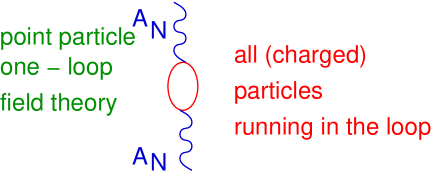
On the other hand, in superstring theory with D–branes the corresponding one–loop gauge threshold effect $\Delta_{a}$ arises from a cylinder diagram with its two boundaries attached to D$p$– and D$p^{\prime}$–branes. On one of them the two gauge vectors $A_{M}$ of the gauge group $G_{a}$ under consideration couple to the closed loop (for anomaly free gauge group), c.f. Figure 18. Hence one of the D–branes must carry the gauge group $G_{a}$ under consideration. In addition, there is a Möbius diagram starting and ending at the same D–brane. In other words, the Möbius diagram may be understood as a cylinder with one boundary attached to the D$p$–brane with gauge group $G_{a}$, where the two gauge fields couple and the second boundary representing a crosscap attached to an orientifold O–plane (c.f. Figure 18). On the other hand, since neither the Klein bottle nor the torus worldsheet have boundaries, where gauge fields from the branes could couple, these diagrams do not contribute to one–loop gauge threshold corrections.

Figure 18: One–loop gauge threshold effects in string theories with D–branes.

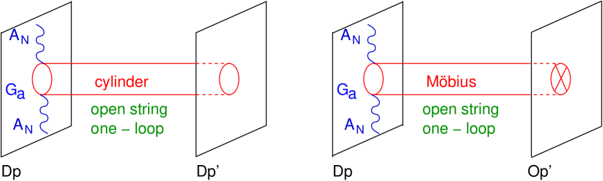
In a generic string background with ${\cal N}=2$ SUSY in $D=4$ the gauge kinetic terms are 1/2 BPS protected, which means that only 1/2 BPS states contribute in the one–loop diagram. Furthermore, in that case the gauge kinetic function does not receive any further corrections beyond one–loop. Though this is a special case, since only a subset of the charged states of the spectrum contributes in the loop, it is a more generic property, which also holds in theories with ${\cal N}=1$ SUSY in $D=4$.

The gauge threshold corrections $\Delta_{a}$ for a gauge group $G_{a}$ are given by a (weighted) sum over the masses of charged particles running in the loop. This effect may be written as a Schwinger type integral

$$\Delta_{a}=\int_{\epsilon}^{\infty}\ {\frac{dt}{t}}\ {\rm Tr}^{\prime}\ (-1)^{F}\ F\ e^{-t\ M^{2}}\ ,$$ (4.181)

with some UV–regularization $\epsilon$. The masses $M$ depend on the geometry of the underlying compactification manifold ${\cal X}$. Indeed, in a more geometric language, the gauge threshold corrections $\Delta_{a}$ are determined by a topological invariant of the compactification manifold ${\cal X}$, namely the analytic Ray–Singer torsion of the manifold ${\cal X}$ [392]. The latter is computed explicitly based on topological arguments, see [393, 394, 395] for examples in heterotic string theory or [396] in heterotic M–theory. As an example, let us discuss type I superstring theory compactified on $K3\times\mathbb{T}^{2}$ with D9–branes comprising the gauge group $G_{a}$ (in addition for consistency, there is a set of D5–branes). In that case the gauge kinetic term is a 1/2 BPS protected quantity depending on the vectormultiplet moduli only (c.f. subsection 4.3.2 for a detailed account on that moduli space). For the background $K3\times\mathbb{T}^{2}$ we shall evaluate the integral (4.181), which boils down to a sum over all Kaluza–Klein masses with respect to the torus $\mathbb{T}^{2}$. The latter has the Kähler modulus $t$, the complex structure $u$ and non–trivial Wilson lines $a_{1},a_{2}$. In terms of the latter the Kaluza–Klein BPS–masses of the open strings are given by:

$$\alpha^{\prime}\ M_{KK}^{2}={\frac{1}{t_{2}u_{2}}}\ |m_{1}+a_{1}+u\ (m_{2}+a_{2})|^{2}\ ,$$

with the integers $m_{1},m_{2}$. Therefore, (4.181) becomes:

$$\Delta_{a} = \int^{\infty}_{0}\ {\frac{dt}{t}}\ \left\{\ \sum_{(m_{1},m_{2})}\ e^{-{\frac{\pi t}{t_{2}u_{2}}}|m_{1}+a_{1}+u(m_{2}+a_{2})|^{2}}-{\frac{t_{2}}{t}}\right\}$$ (4.182)

$$= t_{2}\ \int^{\infty}_{0}\ {\frac{dt}{t^{2}}}\ \sum_{(n_{1},n_{2})\neq(0,0)}\ e^{-{\frac{\pi t_{2}}{tu_{2}}}|n_{1}+un_{2}|^{2}}\ e^{2\pi i(a_{1}n_{2}+a_{2}n_{1})}\ .$$

The second term in the first line of (4.182) is a regularization to remove the state $(m_{1},m_{2})=(0,0)$. The above integral may be evaluated following the techniques presented in [397], with the result [398]:

$$\Delta_{a}=-\ln\left|e^{\pi ia_{2}^{2}u}\ {\frac{{\theta}\left[1/2\atop 1/2\right](a_{1}-u\ a_{2},u)}{\eta(u)}}\right|^{2}\ .$$ (4.183)

The $t$–dependence has dropped out as a result of scale invariance of the integrand (4.182). Indeed, the result (4.183) is the analytic torsion of the genus one torus $\mathbb{T}^{2}$ endowed with the non–trivial background $a_{1},a_{2}$ [392].

In heterotic ${\cal N}=1$ string compactifications, the one–loop threshold correction $\Delta_{a}$ (more precisely the difference of two corrections $\Delta_{a}$ and $\Delta_{a^{\prime}}$ for two different gauge groups $G_{a}$ and $G_{a^{\prime}}$) is related to the closed string topological partition function $F_{1}$ at genus one [399]. Similarly, in type II with D–branes this correction is given by the open string topological partition function $F_{0,2}$, i.e. the open string topological partition function on an annulus [393]. Hence (4.183) is related to the open string topological partition function $F_{0,2}$ [398].

4.6.2 Gauge threshold corrections in type II orientifolds with D–branes

Let us now turn to the concrete results for one–loop threshold corrections in type II orientifolds with D–branes. One–loop threshold corrections $\Delta_{a}$ for type IIB orientifolds with parallel D–branes have been computed in [400, 161, 401, 402], while for type IIA orientifolds with D–branes at angles or for type IIB orientifolds with world volume two–form flux these corrections have been pioneered in [403]. The latter results have been generalized for non–diagonal two–form flux in [404].

The relevant amplitudes to compute at string one–loop are the cylinder and the Möbius amplitude (Figure 18). In type II orientifolds with ${\cal N}=1$ spacetime SUSY in $D=4$ the open strings between a D$p$– and D$p^{\prime}$ or between a D$p$– and one O–plane may preserve $1,1/2$ or $1/4$ of the original 16 supercharges of a type II orientifold in $D=10$, thus giving rise to a ${\cal N}=4,2$ or ${\cal N}=1$ SUSY sector contributing to the gauge threshold corrections, respectively. Since for ${\cal N}=4$ in $D=4$ gauge couplings are not renormalized at one–loop only the $1/2$ and $1/4$ BPS sectors give rise to a non–vanishing contribution to the one–loop gauge threshold corrections in $D=4$.

In IIA orientifold with intersecting D6–branes and O6–planes, the BPS sectors are classified according to the three relative angles $\varphi^{j}_{ba}=\varphi^{j}_{b}-\varphi^{j}_{a},\ j=1,2,3$ between two stacks of D6–branes $a$ and $b$ or between one stack of a D6–brane and an O6–plane. Here $j$ is the $j$–th internal complex direction (c.f. subsection 2.3 for more details). For the case $\varphi_{ba}^{j}=0\ ,j=1,2,3$, i.e. two parallel branes or one brane is parallel to an O6–plane all 16 supercharges are preserved. In that case the corresponding cylinder or Möbius diagram does not give rise to any one–loop threshold effect (${\cal N}=4$ sector).

On the other hand, the ${\cal N}=1$ case $\varphi^{1}_{ba}+\varphi^{2}_{ba}+\varphi^{3}_{ba}=0\ {\rm mod}\ 2\pi$ gives a $1/4$ BPS contribution to the threshold corrections. It has been computed in [403] and gives:

$$\Delta^{{\rm IIA},{\cal N}=1}_{ab}=-b_{ab}^{N=1}\ \ln{\frac{\Gamma(1-{\frac{1}{\pi}}\ \varphi_{ba}^{1})\ \Gamma(1-{\frac{1}{\pi}}\ \varphi_{ba}^{2})\ \Gamma(1+{\frac{1}{\pi}}\ \varphi_{ba}^{1}+{\frac{1}{\pi}}\ \varphi_{ba}^{2})}{\Gamma(1+{\frac{1}{\pi}}\ \varphi_{ba}^{1})\ \Gamma(1+{\frac{1}{\pi}}\ \varphi_{ba}^{2})\ \Gamma(1-{\frac{1}{\pi}}\ \varphi_{ba}^{1}-{\frac{1}{\pi}}\ \varphi_{ba}^{2})}}\ .$$ (4.184)

Here, the index $a$ refers to the D6–brane stack of the gauge group $G_{a}$ under consideration and the index $b$ accounts for any other stack of D6–branes or orientifold planes, with the relative angles obeying $\varphi^{1}_{ba}+\varphi^{2}_{ba}+\varphi^{3}_{ba}=0\ {\rm mod}\ 2\pi$. To obtain all $1/4$ contributions to the gauge threshold correction $\Delta_{a}$, one has to sum over all those stacks $b$ under question. The factor $b_{ab}$ is the corresponding beta–function coefficient accounting for all charged open strings stretched between stack $a$ and $b$ and contributing in the corresponding cylinder or Möbius diagram. Note, that through the angles $\varphi_{ba}^{j}$ (c.f. Eq. (2.262)), the whole expression (4.184) depends on the complex structure moduli.

Furthermore, the ${\cal N}=2$ case occurs, if $\varphi^{k}_{ba}=0$ for one $k$ and $\varphi^{i}_{ba}+\varphi_{ba}^{j}=0\ {\rm mod}\ 2\pi$ for the remaining two relative angles. That case gives rise to a 1/2 BPS contribution to the one–loop threshold corrections. This contribution may be phrased as (4.182), however with a modified mass contributing to the one–loop correction (4.181). More precisely, with respect to the complex plane with $\varphi^{k}_{ba}=0$, the open strings stretched between the two stacks $a$ and $b$, which are parallel in this subplane and each of them carries the wrapping numbers $(p_{a}^{k},q_{a}^{k})$, have non–vanishing Kaluza–Klein momenta and windings. Their mass is given by the mass formula of open strings stretched between two parallel D1–branes, which are wrapped around the torus $T_{2}^{k}$ with wrapping numbers $(p_{a}^{k},q_{a}^{k})$, c.f. Eq. (2.294):

$$\alpha^{\prime}\ M_{KK}^{2}={\frac{u_{2}^{k}}{t_{2}^{k}}}\ {\frac{|n_{k}+m_{k}t^{k}|^{2}}{|p_{a}^{k}+q_{a}^{k}u^{k}|^{2}}}\ .$$ (4.185)

This mass enters the formula (4.181) and we compute [403]:

$$\Delta_{ab}^{{\rm IIA},\rm N=2} = b^{\rm N=2}_{ab}\ {\frac{|p_{a}^{k}+q_{a}^{k}u^{k}|^{2}}{u_{2}^{k}}}\ \int_{0}^{\infty}\ {\frac{dt}{t^{2}}}\ \sum_{(n_{k},m_{k})\neq(0,0)}e^{-{\frac{\pi}{t}}\ {\frac{|p_{a}^{k}+q_{a}^{k}u^{k}|^{2}}{t_{2}^{k}u_{2}^{k}}}\ |m_{k}+n_{k}t^{k}|^{2}}$$ (4.186)

$$= -b_{ab}^{N=2}\ \left[\ln t^{k}_{2}|\eta(t^{k})|^{4}+\ln{\frac{|p_{a}^{k}+q_{a}^{k}u^{k}|^{2}}{u_{2}^{k}}}-\kappa\right]\ ,$$

with the IR regularization constant $\kappa=\gamma_{E}-\ln(4\pi)$. The last two terms of (4.186) are effects of an IR–regularization [397]. Again to obtain all $1/2$ contributions to the gauge threshold correction $\Delta_{a}$, one has to sum over all those stacks $b$, which are parallel to stack $a$ with respect to one complex plane. In the following, let us discuss $T$–duality on the result (4.186). A $T$–duality along the $\vec{\bf e}_{1}$–axis of all two–tori $\mathbb{T}^{2}_{i}$ results in the interchange $t^{i}\leftrightarrow u^{i}$ and the set of O6–planes is converted to a set of a O3/O7–planes. The one–loop correction (4.186) becomes:

$$\Delta^{\rm IIB,\rm N=2}_{ab}=-b_{ab}^{N=2}\ \left[\ln u^{k}_{2}|\eta(u^{k})|^{4}+\ln{\frac{|p_{a}^{k}+q_{a}^{k}t^{k}|^{2}}{t_{2}^{k}}}-\kappa\right]\ .$$ (4.187)

On the other hand, a $T$–duality along $\vec{\bf e}_{2}$–axis of all two–tori $\mathbb{T}^{2}_{i}$ results in the interchange $t^{i}\leftrightarrow-1/u^{i}$ and $u^{i}\leftrightarrow-1/t^{i}$. Thereby the set of O6–planes is converted to a set of a O9/O5–planes and (4.186) becomes:

$$\Delta^{\rm IIB,\rm N=2}_{ab}=-b_{ab}^{N=2}\ \left[\ln u^{k}_{2}|\eta(u^{k})|^{4}+\ln{\frac{|p_{a}^{k}t^{k}-q_{a}^{k}|^{2}}{t_{2}^{k}}}-\kappa\right]\ .$$ (4.188)

Hence Eq. (4.187) is the type IIB analog of Eq. (4.186) for the case of D3/D7– or D7/D7–branes with two–form fluxes and (4.188) corresponds to the D9/D5 case. This case has been studied in great detail in [400, 402]. Recall that in the equations (4.187) and (4.188) the real part of $t^{j}$ is given in terms of the NS background field $b^{j}$, which gives rise to world–volume two–form flux in type IIB, c.f. subsection 2.3.3.

In type IIA with intersecting D6-branes the threshold correction (4.184) from the ${\cal N}=1$ sector depend on the homology classes of the three–cycles (open string parameters) and also on the closed string geometrical moduli. In particular, these functions depend on the complex structure moduli, while in IIB they are functions on the Kähler moduli. The result (4.184) may be easily translated to type IIB orientifolds with two–form fluxes by using the relation (2.213). In the equivalent $T$-dual picture the threshold corrections will be a function of the open string magnetic gauge fluxes and of the geometrical moduli of the dual compact space, i.e. they depend on the Kähler moduli.

The type IIA result (4.186) and the type IIB results (4.187) and (4.188) are reminiscent of the heterotic threshold results in toroidal orbifold compactification, where only ${\cal N}=2$ orbifold sectors give rise to a moduli dependent contribution [405]. On the other hand, in heterotic orbifold compactifications the contributions from ${\cal N}=1$ sectors give rise to a non–moduli dependent constant.

Since the gauge fluxes are directly related to the non-commutativity parameters of the internal torus, we obtain in this way some interesting, new informations for one–loop threshold corrections on non-commutative tori in string theory, a discussion which extends recent results on one–loop corrections on compact non-commutative spaces in the literature.

To conclude this subsection, let us mention, that other research on one–loop string corrections in D–brane models investigates the Kähler potential and the superpotential, see [406, 407] and [408, 409] and Fayet–Iliopoulos terms [410, 181]. Furthermore in [411], four–gluon scattering at one–loop has been investigated. Finally, results for string amplitudes involving a world–sheet with one handle and one boundary have been pioneered in [412, 413, 414].

5 FLUX COMPACTIFICATIONS

All the string compactifications discussed so far, though showing some of the salient features of the SM physics, suffer from two major shortcomings. Their common origin is the existence of, in general, a large number, of the order of $100$, massless scalar fields. These so-called string moduli arise from the possible marginal deformations of the string background, variations of the size of the total internal manifold or submanifolds thereof do not cost any energy. These massless fields would give rise to long distance interactions, which are not observed in nature. As a second issue, the parameters in the effective four-dimensional action depend on the expectation values of these massless fields, i.e. without knowing these string theory cannot be very predictive.

It was demonstrated that in particular non-perturbative effects like gaugino condensation or world-sheet and space-time instanton corrections could in principle lift the deformations and in four-dimensional language generate a potential for the moduli. This would freeze the moduli and potentially give rise to a small number of supersymmetric or non-supersymmetric minima.

More recently, it was realized that there exist solutions to the tree-level string equations of motions in which not only the ten-dimensional metric varies non-trivially along the compact directions, like in Calabi-Yau compactifications, but also some of the other ten-dimensional fields. These solutions involve in particular fluxes for the $p$-form tensor fields which have the power to obstruct flat deformations of Calabi-Yau backgrounds and thus generate a potential. This leads to the freezing of (at least part of) the moduli. The induced potential is believed to be under sufficiently good control to make precise statements about the structure of the set of string vacua that follows (also called the string landscape). As we will discuss in section 6, contrary to earlier expectations, the fluxes give rise to a plethora of stable vacua. By extrapolating this result our universe seems to be by far less unique than initially hoped for.

The subject of flux compactifications has been developed into a very broad subject and there exist two recent review articles on the subject [74, 75]. Flux compactifications started with the heterotic string compactifications with non-vanishing three-form $H$-flux [42] (see also [140]). In many cases the effects of non-vanishing background fluxes can be formulated in terms of an effective superpotential [44, 45, 46, 48, 49, 50]. in the effective ${\cal N}=1$ supergravity action. Moreover, very often background fluxes in string theory can be explained in supergravity by gauging isometries of the underlying scalar moduli spaces respectively in terms of twisted tori compactifications [415, 416, 417, 418, 419, 420, 421, 422, 423, 424, 425, 426, 427, 359, 428, 429] along the lines of Scherk – Schwarz compactifications [430].

Making contact to the other parts of this review, our goal is to provide the framework of how fluxes and D-branes can be consistently coupled together in a single compactification ansatz. This is necessary to obtain supersymmetric models in which moduli are stabilized, making the low energy Lagrangian in principle predictable, and which are still rich enough to contain a realistic open string particle spectrum of non-abelian gauge symmetries and charged chiral matter. Besides preserving space-time supersymmetry, background fluxes can also be part of breaking supersymmetry in the closed string bulk. Coupling fluxes to the D-branes, one can calculate effects of supersymmetry breaking via fluxes on the open string states. In this way soft supersymmetry breaking terms are generated on the world volumes of the D-branes. This will be discussed in subsection 5.5. In subsections 5.3 and 5.6 we discuss how closed string complex structure moduli can be stabilized by background fluxes in type IIB orientifolds, where we also include the effects of a non-perturbative superpotential, which depends on the geometrical Kähler moduli fields. However we do not investigate how open string moduli, related to the embedding of D-branes into the closed string geometry, can be stabilized (see e.g. [358, 359, 431]).

We will restrict ourselves to some central ideas mostly along the lines of the example of three-form fluxes in type IIB string theory as discussed in [432, 49, 433, 50, 433]. This is the situation that is under best control and has been developed primarily in view of applications in string model building. One of the reasons is that the backreaction of the 3-form fluxes is such that the six-dimensional space is still a warped Calabi-Yau space. However, type IIA or heterotic flux compactifications are more difficult to analyze. Here the backreaction of the fluxes is so strong that the underlying geometry is not any longer Calabi-Yau. We will discuss some aspects of type II and heterotic flux compactifications in subsections 5.7 and 5.8. Furthermore it is interesting to see how flux compactifications behave under various geometrical string duality symmetries. For example, concerning mirror symmetry part of this discussion can be found in [434, 416], and for the heterotic/type IIA string duality in [435, 436]. Finally, we will completely omit the subject of non-geometrical fluxes, which recently received a lot of attention [437, 438, 439].

5.1 Fluxes in string compactifications

In generality, we still only allow a background ansatz which preserves four-dimensional Poincaré invariance or the corresponding anti-de Sitter (AdS) or de Sitter (dS) symmetries. Fluxes are non-trivial backgrounds for the anti-symmetric tensor fields strengths, the RR forms in type II and the generic $H_{3}$ present in any ten-dimensional theory. To preserve the symmetries, they can only be along the internal space, or have to fill out the four-dimensional space-time (for which the tensor field needs to be at least a four-form).

For a $p$-form potential $C_{p}$ with field strength $F_{p+1}=dC_{p}$ the Bianchi-identity is $dF_{p+1}=0$. Following a argument similar to Dirac’s derivation of charge quantization, one arrives at the flux quantization conditions. Upon integrating the field strength over a $(p+1)$-dimensional manifold $\Sigma_{p+1}$ without boundary the charge has to be integer,

$$\frac{1}{\ell_{s}^{p}}\int_{\Sigma_{p+1}}F_{p+1}\in\mathbb{Z}\ .$$ (5.1)

Due to the Bianchi identity, the integral only depends on the homology class of $\Sigma_{p+1}$, and since ${\Sigma}_{p+1}$ has no boundaries, only the cohomology class of $F_{p+1}$ is relevant. Thus, one speaks of a $(p+1)-$form flux through the $(p+1)-$cycle $[{\Sigma}_{p+1}]$, the homological class of ${\Sigma}_{p+1}$.

This can be applied to the three-form $H_{3}$ assuming $dH_{3}=0$. Choosing the compactification space $\cal{X}$ to be a six-dimensional compact Calabi-Yau manifold, one can introduce the symplectic, integral basis $(A^{\Lambda},B_{\Sigma})$ of the homology group $H_{3}({\cal X},\mathbb{Z})$ for the three-cycles. These three-cycles are simply Poincaré-dual to the basis of integer harmonic three-forms $({\alpha}_{\Lambda},\beta^{\Sigma})$ that appear in (2.123). One can expand the generic three-form $H_{3}$ in terms of flux quanta $(n^{\Lambda},e_{\Sigma})$ via

$$\frac{1}{\ell_{s}^{2}}\int_{A^{\Lambda}}H_{3}=m^{\Lambda}\ ,\quad\frac{1}{\ell_{s}^{2}}\int_{B_{\Sigma}}H_{3}=e_{\Sigma}\ ,\quad\quad\Lambda,\Sigma=0,\dots,h^{2,1}\ .$$ (5.2)

Hence, $H_{3}$ in terms of the basis $(\alpha_{\Lambda},\beta^{\Sigma})$ reads

$$\frac{1}{\ell_{s}^{2}}H_{3}=m^{\Lambda}\alpha_{\Lambda}-e_{\Sigma}\beta^{\Sigma}\ .$$ (5.3)

Any closed field strength can be written as a linear combination of harmonic forms of proper degree.

The major issue that we turn to in the following is the question under which conditions the string equations of motion and the Killing spinor equations, the supersymmetry conditions, allow solutions when fluxes are present in the background. As mentioned already, the only case where a trustworthy solution to the ten-dimensional equations of motion is known is the case of type IIB orientifolds with three-form flux. We will mostly concentrate on that. To add fluxes into other string backgrounds very often a perturbative approach is used, starting with a Calabi-Yau solution and adding fluxes as small perturbations while ignoring the backreaction of the metric. This approach is justified in the large radius regime where the fluxes become diluted.

5.2 Type IIB with three-form fluxes

As a prototype example, where at least at the supergravity level everything is quite well understood and under reasonable technical control, let us discuss compactifications of the type IIB superstring with background three-form fluxes. As explained in section 2.2.3, both type IIA and IIB string theories contain the two-form field $B_{2}$ together with its field strength $H_{3}=dB_{2}$. In addition type IIB has the RR potentials $C_{0}$, $C_{2}$ and the four-form $C_{4}$. The complexified axio-dilaton ${\tau}$ and the complex three-form $G_{3}$ are often defined as in (2.83). Most of the following discussion is based in the effective ten-dimensional type IIB supergravity action in Einstein frame and with manifest $SL(2,\mathbb{Z})$ invariance written in (2.84).

5.2.1 Three–form fluxes in type IIB orientifolds

Let us, before going through the details, first summarize some general aspects of type IIB orientifold compactifications with three-form fluxes. The relevant three-form background fields in IIB are $H_{3}$ and $F_{3}$ of section 2.2.3. Note that the Bianchi identity of $F_{3}$ is

$$dF_{3}=-dC_{0}\wedge dB_{2}=-F_{1}\wedge H_{3}\ .$$ (5.4)

Only after setting $F_{1}=0$ we can expand $F_{3}$ in the very same manner in the cohomological basis used in (5.2),

$$\frac{1}{\ell_{s}^{2}}\int_{A^{\Lambda}}F_{3}=\tilde{m}^{\Lambda}\ ,\quad\frac{1}{\ell_{s}^{2}}\int_{B_{\Sigma}}F_{3}=\tilde{e}_{\Sigma}\ ,\quad\quad\Lambda,\Sigma=0,\dots,h^{2,1}\ .$$ (5.5)

This expansion is however only valid in IIB before passing to the orientifold.

The orientifold projections (4.12) and (4.13) put further restrictions on the internal components that can appear. For the orientifold projection (4.12), both $F_{3}$ and $H_{3}$ are elements of $H_{-}^{3}({\cal X})$, while for (4.13) $F_{3}$ is in $H_{+}^{3}({\cal X})$, and $H_{3}$ in $H_{-}^{3}({\cal X})$ (c.f. subsections 4.2.3 and 4.2.4). This leads to a modification of the expansion in harmonics compared to (5.2) or (5.5). Let us first discuss the orientifold projection (4.12). The two three-forms $F_{3},\,H_{3}$ can be organized in terms of $G_{3}$ from (2.83) which also involves the dilaton ${\tau}$. The flux $G_{3}$ is now expanded in a symplectic integral basis of $H^{3}_{-}({\cal X},\mathbb{Z})$

$${G_{3}\over\ell_{s}^{2}}=\sum_{\lambda=0}^{h^{2,1}_{-}}m^{\lambda}\alpha_{\lambda}-e_{\lambda}\beta^{\lambda}\ ,$$ (5.6)

with the $2h^{2,1}_{-}({\cal X})+2$ complex flux parameters $(m^{\lambda},e_{\lambda})$. On the other hand, for the orientifold action (4.13) we have:

$${F_{3}\over\ell_{s}^{2}}=\sum_{\gamma=0}^{h^{2,1}_{+}({\cal X})}m^{\gamma}\alpha_{\gamma}-e_{\gamma}\beta^{\gamma}\ \ \ ,\ \ \ {H_{3}\over\ell_{s}^{2}}=\sum_{\lambda=1}^{h^{2,1}_{-}({\cal X})}m^{\lambda}\alpha_{\lambda}-e_{\lambda}\beta^{\lambda}\ ,$$ (5.7)

with $2(h^{2,1}_{+}({\cal X})+2)$ real flux parameters $(m^{\gamma},e_{\gamma})$ for $F_{3}$ and in the same way $(m^{\lambda},e_{\lambda})$ for $H_{3}$. These are the three-form fluxes that can exist in a IIB orientifold background as a matter of principle. The existence of an actual solution to the (classical) equations of motion with a compact internal space then justifies their appearance in orientifold compactifications.

Let us start with a list of qualitative consequences of these fluxes in string compactifications. Afterwards we will elaborate on each of the points in much more detail.

• As local conditions for supersymmetry the ten-dimensional Killing spinor equations, the variations of the gravitinos and dilatino $\delta\psi_{M}=0$ and $\delta\lambda=0$ are modified in the presence of three-form fluxes. As a result the metric is not even of the form (2.59), i.e. four-dimensional Minkowski space times an internal Ricci-flat space, instead a non-trivial warp factor appears in the metric like in (2.98).

• In the classical supergravity equations of motion the background fluxes $H_{3}$ and $F_{3}$ provide extra source terms, such as in the Einstein equations with a general warped metric ansatz in (2.2.5). Thus, it also follows from the equations of motion, not even regarding supersymmetry, that the internal metric is no longer Ricci-flat. This implies that the deformations of the former Calabi-Yau metric are at least partially obstructed by the fluxes.

• Via CS terms in the ten-dimensional action (2.84) the three-form fluxes act as sources for the four-form potential $C_{4}$. They modify the topological charge cancellation condition analogous to (2.95), as can be read from the modified Bianchi identity of the five-form field strength

  $$dF_{5}=-dC_{2}\wedge dB_{2}=H_{3}\wedge F_{3}\ .$$ (5.8)

  Thus, the three-form fluxes effectively carry the charge of a number of D3-branes as determined by the integral of (5.8). The supersymmetry conditions that we will study in a moment imply the positivity of the effective charge.

• Dimensional reduction of the ten-dimensional action (2.84) in the presence of three-form fluxes (plus other fields needed to complete the solution) leads to a four-dimensional action with a scalar potential. The relevant terms with three-form flux contributions is the kinetic terms for $G_{3}$ and the CS term. Roughly speaking, the potential depends on the moduli controlling the size of the cycles ${\Sigma}_{3}$ with non-vanishing flux and the dilaton ${\tau}$. Minimizing this scalar potential can potentially fix these moduli fields reflecting the obstruction of metric deformation via fluxes.

• The fluxes also impose new consistency conditions for the world volume theory of D-branes, if present. For instance, the Bianchi identity for the diagonal $U(1)$ gauge field on a D-brane

  $$2\pi{\alpha}^{\prime}d{\cal F}=dB_{2}+2\pi\alpha^{\prime}dF=0$$ (5.9)

  leads to the Freed-Witten anomaly cancellation condition. The flux $H_{3}$ through a three-cycle wrapped by a D-brane has to vanish.

In the following we discuss these points in more detail.

5.2.2 Supersymmetry conditions with fluxes in IIB

Following the recent review article [74], let us discuss the general supersymmetry conditions resulting from the vanishing of the supersymmetry variations of the gravitino and dilatino fields. These are local conditions in ten dimensions that guarantee the existence of Killing spinors in the given background. They lead to a classification of supersymmetric geometries with fluxes, but a compact internal space very often imposes additional constraints that are not covered. Neither is always known if compact solutions of the described type actually exist. Again, the simplest scenario of the type IIB Calabi-Yau orientifold with three-form flux is an exception that can be constructed on top of any Calabi-Yau space.

For the ten-dimensional metric one can use the general warped ansatz (2.98). The four-dimensional metric $g_{\mu\nu}$ describes either a Minkowski, de Sitter (dS₄), or anti-de Sitter (AdS₄) space. In general other bosonic fields are also allowed to acquire non-trivial profiles and vacuum expectation values in the background, but all fermion fields vanish.

In ten space-time dimensions the type II supersymmetry variations for the two gravitinos $\psi_{M}^{A}$ ($A=1,2)$ and the two dilatinos take the following form (in string frame)

$$\delta\psi_{M} = \nabla_{M}\epsilon+\frac{1}{4}/\!\!\!\!{H_{M}}\mathcal{P}\epsilon+\frac{1}{16}e^{\Phi}\sum_{n}/\!\!\!\!{F_{n}}\Gamma_{M}\mathcal{P}_{n}\epsilon\ ,$$

$$\delta\lambda = /\!\!\!{\partial}\Phi\epsilon+\frac{1}{2}/\!\!\!\!{H}\mathcal{P}\epsilon+\frac{1}{8}e^{\Phi}\sum_{n}(-1)^{n}(5-n)/\!\!\!\!{F_{n}}\mathcal{P}_{n}\epsilon\ .$$ (5.10)

Here the spinors $\psi_{M}$, ${\lambda}$ and ${\epsilon}$ always combine two spinors but we suppress the label $A$. The $\mathcal{P}$ and $\mathcal{P}_{n}$ are $2\times 2$ projection matrices, whose form we do not need explicitly. For more details on the notation we always refer to [74]. The vanishing of these variations is required for supersymmetry. The number of Killing spinors $\epsilon$ determines the number of supercharges that are preserved. It is now evident that without fluxes and with constant dilaton the solutions are just the covariantly constant spinors of the Calabi-Yau, while fluxes and dilaton profiles turn the conditions into much more complicated looking differential equations.

To examine the constraints, we can decompose the ten-dimensional spinors into tensor products of four- and six-dimensional spinors,

$$\epsilon^{A}_{\rm IIB}(x^{M})=\xi^{A}_{+}(x^{\mu})\otimes\eta_{+}(x^{i})+\xi^{A}_{-}(x^{\mu})\otimes\eta_{-}(x^{i})\ .$$ (5.11)

Supersymmetry in the absence of fluxes thus leads to the constraint (2.219) implying reduced holonomy for the internal space, from $SO(6)\simeq SU(4)$ to $SU(3)$, so that ${\cal X}$ is a Calabi-Yau manifold. The two covariantly constant spinors of type II theories of course lead to ${\cal N}=2$ supersymmetry in four dimensions. With non-vanishing fluxes $\eta_{\pm}$ can be viewed as covariantly constant with respect to a new connection $\nabla^{\prime}$ different from the Levi-Civita connection. The internal manifold will no longer have $SU(3)$ holonomy (with respect to the Levi-Civita connection). Instead, the requirement of having $SU(3)$ holonomy with respect to the new connection means that the six-dimensional internal manifold has a so-called $SU(3)$ group structure, i.e. the transition functions of the frame bundle take values in an $SU(3)\subset SO(6)$ subgroup.

This allows to decompose spinors and forms of the internal six-dimensional manifold with respect to their transformation properties under $SU(3)$. One finds that there exist a non-vanishing real two-form $J_{2}$ and a complex three-form $\Omega_{3}$ like on a Calabi-Yau. Moreover, these forms can be related to spinors $\eta_{\pm}$ in the following way (we have set $\ell_{s}=1$),

$$(J_{2})_{ij} = \mp 2i\eta^{\dagger}_{\pm}{\Gamma}_{ij}\eta_{\pm}\ ,$$

$$(\Omega_{3})_{ijk} = -2i\eta_{-}^{\dagger}{\Gamma}_{ijk}\eta_{+}\ .$$ (5.12)

While these forms are closed on a Calabi-Yau, this is now no longer the case. Their deviation from being closed is measured by what is called torsion. The classification of the different classes of torsion under $SU(3)$ helps in understanding the properties of the underlying geometry [440]. The exterior derivative of $J_{2}$ and $\Omega_{3}$ can be expressed using these torsion classes

$$dJ_{2} = \frac{3}{2}\textrm{Im}(\overline{\cal W}_{1}\Omega_{3})+{\cal W}_{4}\wedge J_{2}+{\cal W}_{3}\ ,$$

$$d\Omega_{3} = {\cal W}_{1}J_{2}\wedge J_{2}+{\cal W}_{2}\wedge J_{2}+\overline{\cal W}_{5}\wedge\Omega_{3}\ .$$ (5.13)

Here ${\cal W}_{1}$ is a complex scalar, ${\cal W}_{2}$ a complex primitive $(1,1)$-form, ${\cal W}_{3}$ a real primitive three-form built out of $(2,1)+(1,2)$-forms, ${\cal W}_{4}$ a real vector, and ${\cal W}_{5}$ is a complex $(1,0)$-form.

A manifold with $SU(3)$ structure is complex if ${\cal W}_{1}={\cal W}_{2}=0$ and symplectic if ${\cal W}_{1}={\cal W}_{3}={\cal W}_{4}=0$. A Kähler manifold is at the same time complex and symplectic, and therefore the only non-zero torsion class can be ${\cal W}_{5}$. Finally for a Calabi-Yau manifold with $SU(3)$ holonomy all five torsion classes are zero.

Since the connection and the torsion depend on the fluxes, the above conditions on the torsion classes can be translated into conditions on fluxes. A detailed analysis for ${\cal N}=1$ solutions in type IIB with both RR and NSNS three-form fluxes $H_{3}$ and $F_{3}$, yields three different classes

$$\left.\begin{array}[]{lc}{\rm Type\ A}:&dJ_{2}\pm iH_{3}\\ {\rm Type\ B}:&F_{3}\mp ie^{-\Phi}H_{3}\\ {\rm Type\ C}:&d(e^{-\Phi}J_{2})\pm iF_{3}\end{array}\right\}{\rm is~{}(2,1)~{}and~{}primitive}\ .$$ (5.17)

On a Calabi-Yau the $(2,1)$-forms are automatically primitive, so there is no extra condition. For extended supersymmetry, such as for instance in case of a flat torus, there are additional $(2,1)$-forms such as $dz\wedge J_{2}$ which are not primitive.

In the following we will be mainly interested in the type B class solutions. They can be reformulated in terms of the complex three-form (2.83), saying that $G_{3}$ is imaginary self dual (ISD) under internal Hodge duality and has no $(0,3)$-component,

$${\rm Type\ B}:\quad\star G_{3}=iG_{3}\ ,\quad G_{3}^{0,3}=0\ .$$ (5.18)

One can now immediately see that this condition (5.18) can fix geometrical moduli, since it depends on the internal metric through the Hodge star operation. However, the Hodge duality in six dimensions is invariant under an overall rescaling of the metric, such that the overall volume of the compactification space is not constrained by (5.18).

In the following we will discuss how the supersymmetry condition are related to the condition for a solution to the equations of motion and to the conditions that follow from extremizing an effective four-dimensional potential after dimensional reduction. It is striking to note at this point that only for the type B case of solutions to the Killing spinor equations actual classes of solutions to the equations of motions are known and an effective four-dimensional approach can be defined. We will later also comment on type IIA and heterotic flux vacua, but we basically leave all other solutions aside.

5.2.3 Compactification with fluxes: equations of motion

In order to start a program of flux compactifications one has to make sure that solutions to the equations of motion exist with an internal space that is actually compact. To preserve supersymmetry, the Killing spinor equations of the previous section also have to be satisfied, in our case the conditions (5.18). The corresponding solution was found by Giddings, Kachru and Polchinski in [49]. We will not go through all details but only explain the logic of the equations and list the result.

To start with, recall the modification of the Bianchi identity (or equation of motion) of the self-dual five-form $F_{5}$ in (5.8). The supersymmetry condition on $G_{3}$ in (5.18) now immediately implies the positivity of the right-hand-side. Integration over the compact internal space leads to a contradiction such that other sources are needed. Anti-branes would be an option at this stage, but in order to preserve ${\cal N}=1$ supersymmetry one has to pass to an orientifold with negative background D3-brane charge. The natural framework is that of type IIB orientifolds of the type with O3/O7-planes and potential D3/D7-branes. Including localized D3-brane and O3-plane charges the Bianchi identity gets modified to

$$dF_{5}=H_{3}\wedge F_{3}+2{\kappa}_{10}^{2}\mu_{3}\sum_{a}\pi_{6}^{a}+2{\kappa}_{10}^{2}Q_{3}\mu_{3}\pi_{6}^{\rm Opl}\ ,$$ (5.19)

where the six-forms $\pi_{6}^{a}$ and $\pi_{6}^{\rm Opl}$ have support at the locations of the branes (labeled again by $a$) and the O3-planes. Integration schematically leads to

$$N_{\rm flux}+N_{\rm D3}+Q_{3}N_{\rm O3}=0\ .$$ (5.20)

where in particular the effective charge induced by fluxes is defined

$$N_{\rm flux}={1\over\ell_{s}^{4}}\int_{\cal X}H_{3}\wedge F_{3}\ .$$ (5.21)

Thus the equation for the five-form imposes the topological charge cancellation condition analogous to (2.95) for the D3-brane charge.

The Einstein equation for the general metric ansatz (2.98) is of the form given in (2.2.5). On the right-hand-side the contribution of the three-form fluxes, the five-form and the dilaton appear. Integration of the component with four-dimensional indices again gives a constraint since the left-hand-side is a total derivative. A solution is found in the following way, for the five-form an ansatz is made

$$F_{5}=(1+*)d{\alpha}\wedge dx^{0}\wedge dx^{1}\wedge dx^{2}\wedge dx^{3}\ ,$$ (5.22)

and the dilaton is taken to be constant (which is possible in the presence of only D3-branes without D7-branes). One can then combine the Einstein equation with (5.19) and finds a solution under the following restrictions on the closed string background fields,

$$\star G_{3}=iG_{3}\ ,\quad{\Delta}^{-2}={\alpha}\ ,\quad\Phi={\rm const}\ .$$ (5.23)

In other words, the warp factor is given by the five-form and the three-form flux has to be ISD. The remaining Einstein equation for the internal components becomes equivalent to the equation of the five form if the internal metric without the warp factor is Ricci-flat. The internal space is therefore a conformal Calabi-Yau manifold, i.e. a Calabi-Yau manifold only up to the warp factor. This is very good news, since we know such manifolds do exist, we know their moduli spaces, and also how to perform dimensional reduction on such a background.

It is important to note that (5.23) are precisely the supersymmetry conditions of the type B solution in type IIB, except for the missing constraint that $G^{0,3}=0$ from (5.18). Thus, ISD three-form flux of Hodge type $(0,3)$ can break supersymmetry without destroying the solution.

5.2.4 The effective four-dimensional potential

Let us now investigate the type IIB orientifold flux compactifications based on the solution of the previous section from a four-dimensional perspective. We mainly concentrate on the derivation of the scalar potential.

A complication in such an approach is the presence of the non-trivial warp factor in the metric (2.98). In principle, one expects that terms from the ten-dimensional action with internal derivatives in the reduction contribute, i.e. that ${\alpha}^{\prime}$ corrections are getting important due to the dependence of the warp factor on the internal coordinates. This effect is usually treated as a small effect and neglected which is justified by the scaling of the warp factor with the inverse total volume of the internal space. At sufficiently large volume effects of warping are believed to be controllably small, at least away from sources and regions of strong warping, so-called throats. We will also follow this philosophy and implicitly set ${\Delta}$ to a constant.

The easiest way to obtain a potential from fluxes is to just naively insert a reduction ansatz into the ten-dimensional kinetic action of $G_{3}$. It is given by the following expression

$${\cal V}_{\rm kin}={1\over 4\kappa_{10}^{2}{{\rm Im}}\,{\tau}}\int_{\cal X}G_{3}\wedge\star\bar{G}_{3}\ .$$ (5.24)

Here $G_{3}$ only refers to the background flux and no fluctuations of the two-forms are included. In type IIB these would be present but in the O3/O7 orientifold both $C_{2}$ and $B_{2}$ are projected out of the spectrum. Using that $\star^{2}G_{3}=-G_{3}$ one can now split the three-form flux into an imaginary self-dual piece $G_{3}^{+}$ and an imaginary anti-self-dual piece $G_{3}^{-}$, defined by

$$\star G_{3}^{\pm}=\pm iG_{3}^{\pm}\ .$$ (5.25)

After some algebra one finds that

$${\cal V}_{\rm kin}={1\over 2\kappa_{10}^{2}{{\rm Im}}\,{\tau}}\int_{\cal X}G^{-}_{3}\wedge\star\bar{G}^{-}_{3}-{i\over 4\kappa_{10}^{2}{{\rm Im}}\,{\tau}}\int_{\cal X}G_{3}\wedge\bar{G}_{3}\ ,$$ (5.26)

The second term is equal to $\mu_{3}N_{\rm flux}$. When the vacuum energy of the localized sources, the tension of the D3-branes and O3-planes is added to the full potential, one can make use of the charge cancellation condition (5.19) to cancel these against the second term of (5.26). It turns out that these contributions can be interpreted as D-terms in the effective theory as we have already seen at various instances for the tension of brane systems. Their cancellation is thus a D-flatness condition. Thus the full potential energy is then given as

$${\cal V}={\cal V}_{\rm kin}+{\cal V}_{\rm DBI}={1\over 2\kappa_{10}^{2}{{\rm Im}}\,{\tau}}\int_{\cal X}G^{-}_{3}\wedge\star\bar{G}^{-}_{3}\ .$$ (5.27)

It is positive definite and can be written as an F-term in the effective theory. Obviously, the potential has global minima whenever $G_{3}^{-}=0$, which is the condition that also followed from the ten-dimensional equations of motion in (5.23).

One can now reproduce the structure of a standard supergravity F-term scalar potential as in (2.108). The superpotential is of the Gukov-Taylor-Vafa-Witten type [44, 45, 46]

$$W=\frac{1}{{\kappa}_{10}^{2}}\int_{\cal X}G_{3}\wedge\Omega_{3}\ ,$$ (5.28)

which depends only on the complex structure moduli encoded in ${\Omega}_{3}$, and on the dilaton ${\tau}$ inside $G_{3}$. The Kähler potential of the background Calabi-Yau was given in (2.118), (2.119) and (2.120). The use of this Kähler potential is of course not fully accurate since there exist corrections already at the classical level through the fluxes. We still use it in a heuristic fashion, following [45].

For an orientifold with O3/O7–planes $\Omega_{3}\in H^{3}_{-}({\cal X})$ and $G_{3}\in H^{3}_{-}({\cal X})$. The expansion of ${\Omega}_{3}$ in the Calabi-Yau itself from (2.2.6) then needs to be truncated to odd harmonic three-forms. The analogous expansion of $G_{3}$ was given in (5.6). Since $W$ does not depend on the Kähler moduli, the remaining sum over these in the term $G^{{\alpha}{\bar{\beta}}}{\cal K}_{\alpha}{\cal K}_{\bar{\beta}}|W|^{2}$ in (2.108) cancels against the $-3|W|^{2}$. This condition,

$$G^{A\bar{B}}{\cal K}_{A}{\cal K}_{\bar{B}}=3\ ,$$ (5.29)

$A,\bar{B}$ labeling Kähler moduli only, is the so-called no-scale structure of the classical Kähler potential on a Calabi-Yau. It was shown in [441] that $\alpha^{\prime}$ corrections to the Kähler potential for the Kähler moduli break the no-scale structure (see also [442, 443]). Using labels $I,\bar{J}$ collectively for the remaining complex structure moduli and the dilaton the F-term potential is

$${\cal V}=\kappa^{2}_{4}\,e^{{{\kappa}^{2}_{4}\cal K}}G^{I\bar{J}}D_{I}WD_{\bar{J}}\bar{W}\ .$$ (5.30)

This expression is positive definite and agrees with the first term in (5.27).

Unbroken ${\cal N}=1$ supersymmetry now requires the vanishing of the F-terms. Writing $F_{\tau},\,F_{T^{A}}$ and $F_{U^{I}}$ for the F-terms of the dilaton, the Kähler and the complex structure moduli, the constraints are

$$\begin{array}[]{ccc}D_{T^{A}}W=(\partial_{T^{A}}{\cal K})\int_{\cal X}G_{3}\wedge\Omega_{3}=0&\Leftrightarrow&G_{3}^{0,3}=0\ ,\\[11.38092pt] D_{{\tau}}W={1\over{\tau}-\bar{\tau}}\int_{\cal X}\bar{G}_{3}\wedge\Omega_{3}=0&\Leftrightarrow&G_{3}^{3,0}=0\ ,\\[11.38092pt] D_{U^{I}}\,W=\int_{\cal X}G_{3}\wedge\chi_{I}=0&\Leftrightarrow&G_{3}^{1,2}=0\ ,\end{array}$$ (5.34)

where the $\chi_{I}$ denote a basis of odd $(2,1)$-forms. The only component which survives is $G_{3}^{2,1}$. These are absolute minima of the scalar potential with vanishing vacuum energy and supersymmetric solutions to the ten-dimensional equations of motion (if suitably completed with solution for $F_{5}$, a constant dilaton and the warped metric). Only up to the warp factor, the groundstate is always a four-dimensional Minkowski space-time.

Simple counting shows that to set all F-terms to zero one has $2h_{-}^{2,1}+4$ real equations compared to $2h_{-}^{2,1}+2$ real parameters in (${\tau},U^{I}$) to solve for. The system of equations is heavily over-constrained and for general fluxes there are no solutions.

We have so far ignored the D-term constraint for the cancellation of the tension of the branes against the topological contribution of the fluxes, the second term in (5.26). In case of D3-branes only, there is no extra condition, since their tension (in four-dimensional Einstein frame) only depends on the overall volume of the internal space which is unconstrained. This goes along with the fact that $G_{3}$ is automatically primitive on a Calabi-Yau. Instead, for $H^{1}({\cal X})\neq 0$ the additional supersymmetry condition $J_{2}\wedge G_{3}=0$ imposes a non-trivial constraint on the Kähler moduli. This can be demonstrated in toy model orientifold flux compactifications on $\mathbb{T}^{6}$ for example [415, 419].

Coming back to (5.17) the type IIB supersymmetry conditions can be also satisfied by three-form fluxes, for which $G_{3}$ is not ISD (type A and type C class solutions). Here the back-reaction on the internal geometry is qualitatively more severe in the sense that ${\cal X}$ is not anymore a warped CY space. Furthermore, no explicit solution to the equations of motion along the lines outlined in section 5.2.3 is known. Nevertheless there are proposals for effective superpotentials also for these cases. They involve the piece $dJ_{2}$ which is non-vanishing due to torsion but no NSNS three-form flux,

$$W=\frac{1}{{\kappa}_{10}^{2}}\int_{\cal X}(e^{-\Phi}dJ_{2}+F_{3})\wedge\Omega_{3}\ .$$ (5.35)

This type of effective superpotential is believed to be relevant for orientifolds with O5/O9-planes instead of O3/O7-planes. The idea is that the F-flatness conditions of this superpotential reproduce the supersymmetry constraints of the ten-dimensional Killing spinor equations. But the difficulty is to identify the proper moduli with respect to which one should perform a variation and to justify the procedure by an explicit compact solution.

5.3 Three–form fluxes in type IIB $\mathbb{Z}_{N}$ and ${\mathbb{Z}_{N}\times\mathbb{Z}_{M}}$ orientifolds

After going through the general foundations of type IIB orientifold flux compactifications, we now provide a detailed treatment of a class of examples in which the process of moduli stabilization can be studied particularly well.

In this subsection we discuss the flux space for the toroidal $\mathbb{Z}_{N}$ and $\mathbb{Z}_{N}\times\mathbb{Z}_{M}$ orbifolds (4.50). On a six–torus $\mathbb{T}^{6}$ we have $h^{2,1}(\mathbb{T}^{6})=9$, thus ${\rm dim}H^{3}(\mathbb{T}^{6})=20$. We introduce the six real periodic coordinates $x^{i},y^{i}$ on the torus $\mathbb{T}^{6}$, i.e. $x^{i}\cong x^{i}+1$ and $y^{i}\cong y^{i}+1$, $i=1,2,3$. Furthermore we define the following basis

$$\ell_{s}^{3}\,\alpha_{0} = dx^{1}\wedge dx^{2}\wedge dx^{3}\ \ \ ,\ \ \ \ell_{s}^{3}\,\beta^{0}=dy^{1}\wedge dy^{2}\wedge dy^{3}\ ,$$ (5.36)

$$\ell_{s}^{3}\,\alpha_{1} = dy^{1}\wedge dx^{2}\wedge dx^{3}\ \ \ ,\ \ \ \ell_{s}^{3}\,\beta^{1}=-dx^{1}\wedge dy^{2}\wedge dy^{3}\ ,$$ (5.37)

$$\ell_{s}^{3}\,\alpha_{2} = dx^{1}\wedge dy^{2}\wedge dx^{3}\ \ \ ,\ \ \ \ell_{s}^{3}\,\beta^{2}=-dy^{1}\wedge dx^{2}\wedge dy^{3}\ ,$$ (5.38)

$$\ell_{s}^{3}\,\alpha_{3} = dx^{1}\wedge dx^{2}\wedge dy^{3}\ \ \ ,\ \ \ \ell_{s}^{3}\,\beta^{3}=-dy^{1}\wedge dy^{2}\wedge dx^{3}\ ,$$ (5.39)

$$\ell_{s}^{3}\,\gamma_{1} = dx^{1}\wedge dy^{1}\wedge dx^{2}\ \ \ ,\ \ \ \ell_{s}^{3}\,\delta^{1}=-dy^{2}\wedge dx^{3}\wedge dy^{3}\ ,$$ (5.40)

$$\ell_{s}^{3}\,\gamma_{2} = dx^{1}\wedge dy^{1}\wedge dx^{3}\ \ \ ,\ \ \ \ell_{s}^{3}\,\delta^{2}=-dx^{2}\wedge dy^{2}\wedge dy^{3}\ ,$$ (5.41)

$$\ell_{s}^{3}\,\gamma_{3} = dx^{1}\wedge dx^{2}\wedge dy^{2}\ \ \ ,\ \ \ \ell_{s}^{3}\,\delta^{3}=-dy^{1}\wedge dx^{3}\wedge dy^{3}\ ,$$ (5.42)

$$\ell_{s}^{3}\,\gamma_{4} = dx^{2}\wedge dy^{2}\wedge dx^{3}\ \ \ ,\ \ \ \ell_{s}^{3}\,\delta^{4}=-dx^{1}\wedge dy^{1}\wedge dy^{3}\ ,$$ (5.43)

$$\ell_{s}^{3}\,\gamma_{5} = dx^{1}\wedge dx^{3}\wedge dy^{3}\ \ \ ,\ \ \ \ell_{s}^{3}\,\delta^{5}=-dy^{1}\wedge dx^{2}\wedge dy^{2}\ ,$$ (5.44)

$$\ell_{s}^{3}\,\gamma_{6} = dx^{2}\wedge dx^{3}\wedge dy^{3}\ \ \ ,\ \ \ \ell_{s}^{3}\,\delta^{6}=-dx^{1}\wedge dy^{1}\wedge dy^{2}\ ,$$ (5.45)

for the integer cohomology class $H^{3}(\mathbb{T}^{6},\mathbb{Z})$ with respect to ambient space $\mathbb{T}^{6}$. This basis enjoys the following intersection properties (with the choice of orientation $\int_{\cal X}dx^{1}\wedge dx^{2}\wedge dx^{3}\wedge dy^{1}\wedge dy^{2}\wedge dy^{3}=l_{s}^{6}$):

$$\int_{\mathbb{T}^{6}}\alpha_{i}\wedge\beta^{j}=\delta^{j}_{i}\ \ \ ,\ \ \ \int_{\mathbb{T}^{6}}\gamma_{i}\wedge\delta^{j}=\delta^{j}_{i}\ .$$ (5.46)

Before the orbifold projection, there are $20+20$ independent real components for $H_{ijk}$ and $F_{ijk}$. Hence the general three-form flux may be expanded with respect to that basis (5.36):

$${1\over\ell_{s}^{2}}{G_{3}}=\sum_{i=0}^{3}\left[(a^{i}+iS\ c^{i})\alpha_{i}+(b_{i}+iS\ d_{i})\beta^{i}\right]+\sum_{j=1}^{6}\left[(e^{j}+iS\ g^{j})\gamma_{j}+(f_{j}+iS\ h_{j})\delta^{j}\right]\ .$$ (5.47)

The coefficients $a^{i},\ b_{i},\ e^{i},\ f_{i}$ refer to the Ramond part of $G_{3}$, while the coefficients $c^{i},\ d_{i},\ g^{i},\ h_{i}$ refer to its Neveu-Schwarz part.

Under the involution $\sigma^{\ast}=I_{6}$ (Eq. (4.12)) all $20$ untwisted three-forms (5.36) pick up a minus sign, i.e. belong to the cohomology $H^{3}_{-}(\mathbb{T}^{6}/\sigma,\mathbb{Z})$. Hence in that case all $20$ forms (5.36) may give rise to flux components for both $F_{3}$ and $H_{3}$. On the other hand, under the second involution $\sigma^{\ast}=1$ (Eq. (4.13)) all $20$ untwisted three-forms (5.36) are inert, i.e. belong to the cohomology $H^{3}_{+}(\mathbb{T}^{6}/\sigma,\mathbb{Z})$. Hence, $H_{3}=0$ and only $F_{3}$ may receive contributions from all $20$ elements (5.36) [423].

Let us now discuss the effect of the orbifold action (4.51). Only a portion of the forms (5.36) is invariant under the orbifold group $\Gamma$. First of all, the three-forms $\gamma_{i}$ and $\delta^{j}$ are never invariant under the orbifold twist $\Gamma$ as a result, that those forms have two legs from the same complex plane. However they play an important role in constructing a twist invariant basis of three-forms. The number of untwisted flux components of $F_{3},H_{3}$ subject to the orbifold action (4.51) and the orientifold involutions (4.12) or (4.13) is given by the Hodge number $h_{\rm untwist.}^{2,1}({\cal X})$ of the original orbifold ${\cal X}$. For details, see Eq. (4.52) for the involution $\sigma^{\ast}=I_{6}$ and Eq. (4.53) for the involution $\sigma^{\ast}=1$, respectively. Hence, for the orientifold action (4.12) the flux $G_{3}$ has $2h_{\rm untwist.}^{2,1}({\cal X})+2$ untwisted complex components, while the action (4.13) allows only for components of $F_{3}$ and $H_{3}=0$.

The untwisted three-forms, invariant under the orbifold action (4.51) may be most conveniently found in the complex basis, in which the orbifold group $\Gamma$ acts diagonally by the representation (4.51) on the complex basis $\{z^{i}\}$. To pass from the real basis (5.36) to a complex basis, one introduces complex structures, i.e. defines the complex coordinates:

$$dz^{j}=\sum_{i=1}^{3}\ \rho^{j}_{i}\ dx^{i}+\tau^{j}_{i}\ dy^{i}\ \ \ ,\ \ \ j=1,2,3\ .$$ (5.48)

Most of the parameters $\rho^{j}_{i}$ and $\tau^{j}_{i}$ are fixed through the orbifold twist $\Gamma$ [347], with only those remaining undetermined, which correspond to the $\mathbb{Z}_{2}$–elements of $\Gamma$. Eventually the latter are fixed through the flux quantization condition. As we shall see in a moment, the specific values of the constants $\rho^{j}_{i}$ and $\tau^{j}_{i}$ are relevant for finding flux solutions. With respect to to the complex coordinates, defined in (5.48), we may introduce the complex three-form cohomology $H^{3}=H^{3,0}\oplus H^{2,1}\oplus H^{1,2}\oplus H^{0,3}$ of the six–torus $\mathbb{T}^{6}$:

$${\ell_{s}^{3}}\,\omega_{A_{0}} = dz^{1}\wedge dz^{2}\wedge dz^{3}\ \ \ ,\ \ \ {\ell_{s}^{3}}\,\omega_{B_{0}}=d\overline{z}^{1}\wedge d\overline{z}^{2}\wedge d\overline{z}^{3}$$ (5.49)

$${\ell_{s}^{3}}\,\omega_{A_{1}} = d\overline{z}^{1}\wedge dz^{2}\wedge dz^{3}\ \ \ ,\ \ \ {\ell_{s}^{3}}\,\omega_{B_{1}}=dz^{1}\wedge d\overline{z}^{2}\wedge d\overline{z}^{3}$$ (5.50)

$${\ell_{s}^{3}}\,\omega_{A_{2}} = dz^{1}\wedge d\overline{z}^{2}\wedge dz^{3}\ \ \ ,\ \ \ {\ell_{s}^{3}}\,\omega_{B_{2}}=d\overline{z}^{1}\wedge dz^{2}\wedge d\overline{z}^{3}$$ (5.51)

$${\ell_{s}^{3}}\,\omega_{A_{3}} = dz^{1}\wedge dz^{2}\wedge d\overline{z}^{3}\ \ \ ,\ \ \ {\ell_{s}^{3}}\,\omega_{B_{3}}=d\overline{z}^{1}\wedge d\overline{z}^{2}\wedge dz^{3}$$ (5.52)

$${\ell_{s}^{3}}\,\omega_{C_{1}} = dz^{1}\wedge d\overline{z}^{1}\wedge dz^{2}\ \ \ ,\ \ \ {\ell_{s}^{3}}\,\omega_{D_{1}}=dz^{1}\wedge d\overline{z}^{1}\wedge d\overline{z}^{2}$$ (5.53)

$${\ell_{s}^{3}}\,\omega_{C_{2}} = dz^{1}\wedge d\overline{z}^{1}\wedge dz^{3}\ \ \ ,\ \ \ {\ell_{s}^{3}}\,\omega_{D_{2}}=dz^{1}\wedge d\overline{z}^{1}\wedge d\overline{z}^{3}$$ (5.54)

$${\ell_{s}^{3}}\,\omega_{C_{3}} = dz^{1}\wedge dz^{2}\wedge d\overline{z}^{2}\ \ \ ,\ \ \ \ell_{s}^{3}\,\omega_{D_{3}}=d\overline{z}^{1}\wedge dz^{2}\wedge d\overline{z}^{2}$$ (5.55)

$${\ell_{s}^{3}}\,\omega_{C_{4}} = dz^{2}\wedge d\overline{z}^{2}\wedge dz^{3}\ \ \ ,\ \ \ {\ell_{s}^{3}}\,\omega_{D_{4}}=dz^{2}\wedge d\overline{z}^{2}\wedge d\overline{z}^{3}$$ (5.56)

$${\ell_{s}^{3}}\,\omega_{C_{5}} = dz^{1}\wedge dz^{3}\wedge d\overline{z}^{3}\ \ \ ,\ \ \ \ell_{s}^{3}\,\omega_{D_{5}}=d\overline{z}^{1}\wedge dz^{3}\wedge d\overline{z}^{3}$$ (5.57)

$${\ell_{s}^{3}}\,\omega_{C_{6}} = dz^{2}\wedge dz^{3}\wedge d\overline{z}^{3}\ \ \ ,\ \ \ {\ell_{s}^{3}}\,\omega_{D_{6}}=d\overline{z}^{2}\wedge dz^{3}\wedge d\overline{z}^{3}\ .$$ (5.58)

In the following two tables we list for all toroidal orbifolds (4.50) those three-forms, which are left invariant under the orbifold action $\Gamma$, defined in (4.51).

$$\ \ G_{3}$$

Table 23: Allowed three-form fluxes for point group $\mathbb{Z}_{N}$.

$$\ \ G_{3}$$

Table 24: Allowed three-form fluxes for point group $\mathbb{Z}_{M}\times\mathbb{Z}_{N}$.

The remaining 12 fluxes of the form $dz^{a}\wedge d\overline{z}^{a}\wedge dz^{b}$ and $dz^{a}\wedge d\overline{z}^{a}\wedge d\overline{z}^{b}$, respectively are always projected out and therefore do not appear in the tables. They are related to the real basis elements $\gamma_{i}$ and $\delta^{j}$. In terms of the complex basis (5.49) the most general three-form flux $G_{3}$ on $\mathbb{T}^{6}$ has 20 complex components and assumes the following expansion

$${1\over\ell_{s}^{2}}\ G_{3}=\sum_{i=0}^{3}(\ A^{i}\ \omega_{A_{i}}+B^{i}\ \omega_{B_{i}}\ )+\sum_{j=1}^{6}(\ C^{j}\ \omega_{C_{j}}+D^{j}\ \omega_{D_{j}}\ )\ ,$$ (5.59)

with the complex coefficients $A^{i},B^{i},C^{j},D^{j}\in\mathbb{C}$. The three-forms $\omega_{A_{i}}$, $\omega_{B_{i}}$ correspond to flux components with all one–forms coming from different planes, while the forms $\omega_{C_{i}}$, $\omega_{D_{i}}$ are flux components with two one–forms coming from the same plane. The latter we have just written down for completeness, as they are projected out in all orbifolds. With (5.48) we may switch from (5.59) to (5.47) and express all $20$ complex coefficients $A^{i},B^{i},C^{j},D^{j}$ in terms of the $40$ real coefficients $a^{i},\ b_{i},\ e^{i},\ f_{i},c^{i},\ d_{i},\ g^{i},\ h_{i}$ or vice versa.

In the $\mathbb{Z}_{2}\times\mathbb{Z}_{2}$ orientifold/orbifold, which allows for the largest number of (untwisted) fluxes components (c.f. [339] and Table 10), all $\omega_{A_{i}}$ and $\omega_{B_{i}}$ remain, whereas in most other orbifolds only the $(3,0)$ and $(0,3)$ components, given by $\omega_{A_{0}}$ and $\omega_{B_{0}}$ survive. In these cases, no supersymmetric $(2,1)$–form flux can be turned on. That the $(0,3)$ and $(3,0)$-flux always survive is obvious, as the $(3,0)$-flux corresponds to the Calabi-Yau 3-form $\Omega_{3}$, which is always present, and the $(0,3)$-flux to its conjugate.

While in the form (5.59), the cohomology structure of $G_{3}$ is manifest, in order to impose the flux quantization (5.2) on $G_{3}$, i.e.

$${\frac{1}{\ell_{s}^{2}}}\int_{C_{3}}F_{3}\in N_{min}\ \mathbb{Z}\ \ \ ,\ \ \ {\frac{1}{\ell_{s}^{2}}}\int_{C_{3}}H_{3}\in N_{min}\ \mathbb{Z}\ ,$$ (5.60)

with some integer $N_{min}$ (depending on the orbifold group $\Gamma$) to be specified in a moment, one has to transform the forms (5.49) into a real basis (5.36). Let us briefly comment on the integers $N_{min}$, introduced in the flux quantization conditions (5.60). It has been pointed out in [444], that there are subtleties for toroidal orientifolds due to additional three-cycles, which are not present in the covering space $\mathbb{T}^{6}$. If some integers are odd, additional discrete flux has to be turned on in order to meet the quantization rule for those three-cycles. We may bypass these problems in the $\mathbb{Z}_{N}$ ($\mathbb{Z}_{N}\times\mathbb{Z}_{M}$)–orientifolds, if we choose the quantization numbers to be multiples of $N_{min}=2N$ ($N_{min}=2NM$) and do not allow for discrete flux at the orientifold planes [445, 446, 447]. Note, that for $h^{2,1}_{\rm twist.}\neq 0$, in addition to the untwisted flux components $H_{ijk}$ and $F_{ijk}$ there may be also NSNS– and RR–flux components from the twisted sector. We do not consider them here. It is assumed, that their quantization rules freeze the twisted complex structure moduli.

Generically one starts with a specific flux choice (5.59), i.e. some choice for the complex numbers $A^{i},B^{i},C^{j},D^{j}$ allowing e.g. only some flux directions. Then one imposes the flux quantization rule (5.60) for the fluxes $F_{3},H_{3}$ with respect to an integral basis. This is achieved by transforming the flux (5.59) with the help of (5.48) into the integral basis (5.47). However, then one realizes that the flux quantization conditions (5.60) may only be fulfilled for specific values of the dilaton $S$ and complex structure moduli $U$. This way flux quantization is related to discrete values for the dilaton and complex structure moduli. This may be also seen dynamically through the superpotential (5.28) (c.f. subsection 5.3.2).

One way one can think of turning on flux on a D$p$-brane is via the generalized Scherk-Schwarz Ansatz:

$$B_{mn}=H_{mnp}\,x^{p}.$$ (5.61)

The index $p$ may run only over the coordinates transversal to the brane, so in the case of a D7-brane, which fills the directions $x_{0},\ldots,x_{7}$ (wrapping the tori $\mathbb{T}_{1}^{2}\times\mathbb{T}_{2}^{2}$), we have

$$B_{mn}^{7}=H_{mn8}\,x^{8}+H_{mn9}\,x^{9}.$$ (5.62)

As $H_{ijk}$ must always have one index equal to either 8 or 9, not all of the 20 possible components are allowed in our case. Not allowed are the fluxes

$$dx^{1}\wedge dy^{1}\wedge dx^{2}\qquad dx^{1}\wedge dy^{1}\wedge dy^{2}$$

$$dx^{1}\wedge dx^{2}\wedge dy^{2}\qquad dy^{1}\wedge dx^{2}\wedge dy^{2}\ .$$ (5.63)

Expressed in complex notation, this would correspond to the fluxes $H_{1\overline{1}2}$, $H_{1\overline{2}2}$, $H_{1\overline{1}\overline{2}}$, $H_{2\overline{1}\overline{2}}$.

For D7-branes wrapping the tori $\mathbb{T}_{1}^{2}\times\mathbb{T}_{3}^{2}$ or $\mathbb{T}_{2}^{2}\times\mathbb{T}_{3}^{2}$, we find similar results. Having a setup of three stacks of D7-branes, one stack not wrapping $\mathbb{T}_{3}^{2}$, one not wrapping $\mathbb{T}_{2}^{2}$, and one not wrapping $\mathbb{T}_{1}^{2}$, we lose 12 of the twenty flux components and are left with fluxes, which have one index on each of the tori.

5.3.1 Example: Three–form fluxes on the $\mathbb{T}^{6}/\mathbb{Z}_{2}\times\mathbb{Z}_{2}$ orientifold

As an example we consider the $\mathbb{T}^{6}/\mathbb{Z}_{2}\times\mathbb{Z}_{2}$ orientifold with the Hodge numbers $h^{1,1}=3$ and $h^{2,1}=51$, c.f. Table 7. Let us discuss the three-form flux $G_{3}$ for the $\mathbb{Z}_{2}\times\mathbb{Z}_{2}$ orbifold with the orientifold action (4.12) [339]. According to Table 20 we have $h_{\rm untw.}^{2,1}({\cal X})=3$. Hence the (untwisted) three-form flux $G_{3}$ has $2h_{\rm untw.}^{2,1}+2h^{3,0}=2\cdot 3+2=8$ complex flux components. The latter correspond to the forms $\omega_{A_{i}}$ and $\omega_{B_{i}}$, with $i=0,\ldots,3$. These eight flux components are related to a linear combination of the primitive elements of the (untwisted) cohomology $H^{3}({\cal X},\mathbb{C})$. After choosing the complex structure

$$dz^{i}=dx^{i}+i\,U^{i}\ dy^{i}\ \ \ ,\ \ \ i=1,2,3$$ (5.64)

we may go back to the flux in the real representation (5.47). With respect to the basis (5.36) the flux $G_{3}$ is expressible as a linear combination of the eight real forms

$$\alpha_{i}\ \ ,\ \ \ \beta^{i}\ \ \ ,\ \ \ i=0,\ldots,3\ ,$$ (5.65)

given in Eq. (5.36). The expansion coefficients correspond to the eight allowed real components

$$H_{135}\ ,\ H_{136}\ ,\ H_{145}\ ,\ H_{146}\ ,\ H_{235}\ ,\ H_{236}\ ,\ H_{245}\ ,\ H_{246}\ ,$$ (5.66)

of the NSNS three-form $H_{3}$ and to the eight possible real components

$$F_{135}\ ,\ F_{136}\ ,\ F_{145}\ ,\ F_{146}\ ,\ F_{235}\ ,\ F_{236}\ ,\ F_{245}\ ,\ F_{246}$$ (5.67)

of the RR three-form $F_{3}$, each. The above three-forms (5.65), which are invariant under the $\mathbb{Z}_{2}\times\mathbb{Z}_{2}$ orbifold symmetry and form a symplectic basis, are Poincaré-dual to the obvious invariant three-cycles on $\mathbb{T}^{6}$.

There are the three moduli, $U^{I}$, $I=1,2,3$, which define the complex structure (5.64) on the orbifold cover $\mathbb{T}^{6}$. The holomorphic three-form

$${1\over\ell_{s}^{3}}\,\Omega_{3}=dz^{1}\wedge dz^{2}\wedge dz^{3}=X^{\Lambda}\alpha_{\Lambda}-F_{\Lambda}\beta^{\Lambda}$$ (5.68)

defines the homogeneous coordinates $X^{\Lambda}$ and the derivatives $F_{\Lambda}=\partial_{\Lambda}F$ of the prepotential

$$X^{0} = 1\ ,\quad\quad F_{0}=iU^{1}\,U^{2}\,U^{3}\ ,$$

$$X^{1} = iU^{1},\quad\quad F_{1}=-U^{2}\,U^{3}\ ,$$

$$X^{2} = iU^{2},\quad\quad F_{2}=-U^{1}\,U^{3}\ ,$$

$$X^{3} = iU^{3},\quad\quad F_{3}=-U^{1}\,U^{2}\ .$$ (5.69)

Therefore the prepotential is given by

$$F={X^{1}X^{2}X^{3}\over X^{0}}=-i\,U^{1}U^{2}U^{3}\ .$$ (5.70)

The Kähler potential is given by

$$\kappa_{4}^{2}\,{K}=-\ln\prod_{I=1}^{3}(U^{I}+\bar{U}^{I})\ ,$$

and finally the superpotential takes the form

$${\ell_{s}^{3}\over 4\pi}\,W = (b_{0}+iS\,d_{0})+(b_{1}+iS\,d_{1})\,iU_{1}+(b_{2}+iS\,d_{2})\,iU_{2}+(b_{3}+iS\,d_{3})\,iU_{3}$$ (5.71)

$$+(a_{1}+iS\,c_{1})\,U_{2}\,U_{3}+(a_{2}+iS\,c_{2})\,U_{1}\,U_{3}+(a_{3}+iS\,c_{3})\,U_{1}\,U_{2}$$

$$-(a_{0}+iS\,c_{0})\,iU_{1}\,U_{2}\,U_{3}.$$

5.3.2 Complex structure and dilaton stabilization through three-form flux

In this subsection we demonstrate how the stabilization of the dilaton and complex structure moduli is achieved dynamically with the superpotential (5.28) for a general three-form flux $G_{3}$. To keep the expressions short we shall discuss orbifolds ${\cal X}$ with $h_{-}^{2,1}({\cal X})=1$. The Kähler potential ${K}_{0}$ for the dilaton and complex structure modulus ($U\equiv U^{3}$) is:

$$\kappa_{4}^{2}\,K_{0}=-\ln(S+\bar{S})-\ln(U+\bar{U})\ .$$ (5.72)

For $h_{-}^{2,1}({\cal X})=1$ there are four complex parameters to parameterize the most general three-form flux $G_{3}$. The contribution of the latter to the tree–level superpotential (5.28) may be written

$${\ell_{s}^{3}\over 4\pi}\,W_{0}=A+B\ S+U\ (C+D\ S)\ ,$$ (5.73)

with four complex numbers $A,B,C,D\in\mathbb{C}$, to specified later. With the resulting $F$–terms

$${\ell_{s}^{3}\over 4\pi}\,\overline{F}^{\overline{S}} = \kappa_{4}^{2}\ \left({\frac{S+\overline{S}}{U+\overline{U}}}\right)^{1/2}\ \left[\ -A+B\ \overline{S}-U\ (C-D\ \overline{S})\ \right]\ ,$$ (5.74)

$${\ell_{s}^{3}\over 4\pi}\,\overline{F}^{\overline{U}} = \kappa_{4}^{2}\ \left({\frac{U+\overline{U}}{S+\overline{S}}}\right)^{1/2}\ \left[\ -A-B\ S+\overline{U}\ (C+D\ S)\ \right]\ ,$$ (5.75)

we may cast the scalar potential

$${\cal V}=g_{S\overline{S}}\ F^{S}\overline{F}^{\overline{S}}+g_{U\overline{U}}\ F^{U}\overline{F}^{\overline{U}}-3\ \kappa_{4}^{2}\ e^{\kappa_{4}^{2}\,{\cal K}_{0}}\ |W_{0}|^{2}$$ (5.76)

into the form:

$${\cal V} = {\frac{1}{(S+\bar{S})(U+\bar{U})}}\ \left[\ |\ A-B\ \overline{S}+U\ (C-D\ \overline{S})\ |^{2}+|\ A+B\ S-\overline{U}\ (C+D\ S)\ |^{2}\right.$$ (5.78)

$$\hskip 85.35826pt\left.-3\ |\ A+B\ S+U\ (C+D\ S)\ |^{2}\ \right]\ \kappa_{4}^{2}{\frac{(4\pi)^{2}}{l_{s}^{6}}}.$$

The extremal points in the moduli space $(S,U)$ are determined by the solutions of the equations $F^{S},F^{U}=0$:

$$s_{2}={\frac{i}{2}}\ {\frac{\overline{B}\ C-B\ \overline{C}-\overline{A}\ D+A\ \overline{D}}{\overline{B}\ D+B\ \overline{D}}}\ \ \ ,\ \ \ u_{2}={\frac{i}{2}}\ {\frac{-\overline{B}\ C+B\ \overline{C}-\overline{A}\ D+A\ \overline{D}}{\overline{C}\ D+C\ \overline{D}}}\ ,$$ (5.79)

and similarly for the real parts $s_{1},u_{1}$.

The three-form flux (5.47) entering (5.28) is given as a linear combination with respect to the integer cohomology basis $\{\alpha_{i},\beta^{i}\}_{i=0,\ldots,3}$ and $\{\gamma_{j},\delta^{j}\}_{j=1,\ldots,6}$, given in Eq. (5.36). This gives rise to 20 real flux components to be constrained by the respective orbifold group $\mathbb{Z}_{N}$ (c.f. subsection 5.3). This allows to express the complex parameters $A,B,C,D$ through the eight integers $a^{0},a^{1},b_{0},b_{1},c^{0},c^{1},d_{0},d_{1}$. For more details c.f. [347]. The F–flatness conditions $F^{S},F^{U}=0$ force the complex structure to align such, that the flux $G_{3}$

$$\hskip-14.22636pt\displaystyle{l_{s}\ G_{3}} = \displaystyle{{\frac{i}{2\ {\rm Re}(U)}}\ \left\{\ \left[\ \overline{A}-\overline{B}\ S+\overline{U}\ (\overline{C}-\overline{D}\ S)\ \right]\ dz^{1}\wedge dz^{2}\wedge dz^{3}\right.}$$ (5.80)

$$- \displaystyle{\left[\ A+B\ S+U\ (C+D\ S)\ \right]\ d\overline{z}^{1}\wedge d\overline{z}^{2}\wedge d\overline{z}^{3}}$$

$$+ \displaystyle{\left[\ A+B\ S-\overline{U}\ (C+D\ S)\ \right]\ d\overline{z}^{1}\wedge d\overline{z}^{2}\wedge dz^{3}}$$

$$- \displaystyle{\left.\left[\ \overline{A}-\overline{B}\ S-U\ (\overline{C}-\overline{D}\ S)\ \right]\ dz^{1}\wedge dz^{2}\wedge d\overline{z}^{3}\ \right\}}$$

corresponding to the choice (5.73) becomes ISD, i.e. it has only $(2,1)$ and $(0,3)$–components at the extremum. The flux $G_{3}$ induces the contribution of

$$N_{\rm flux}={1\over\ell_{s}^{4}}\ \int_{\cal X}F_{3}\wedge H_{3}$$ (5.81)

to the total D3-brane charge (4.71). Generically, this integral is calculated in the orientifold cover ${\cal X}$. Therefore the number $N_{flux}$ has to be twice the negative value of the total D3-brane charge (4.71), i.e.

$$N_{\rm flux}=-2\ Q_{3,tot}$$ (5.82)

to cancel the latter by flux only.

As an example, let us discuss the $\mathbb{Z}_{6-II}$–orbifold with the torus lattice $SU(2)\times SU(6)$ [340]. The $\mathbb{Z}_{6-II}$–orbifold has the action $(v^{1},\,v^{2},\,v^{3})=({1\over 6},\,{1\over 3},\,-{1\over 2})$. The three-form flux (5.47) constrained by the $\mathbb{Z}_{6-II}$–orbifold group becomes:

$$\displaystyle{{\frac{1}{\ell_{s}^{2}}}\ G_{3}} = \displaystyle{{\frac{1}{3}}\ (a_{0}+iSc_{0})\ (3\ \alpha_{0}+2\ \beta_{3}+\gamma_{1}-2\gamma_{2}-2\ \gamma_{3}+\gamma_{4}-\delta_{5})}$$ (5.83)

$$+ \displaystyle{(b_{0}+iSd_{0})\ (-\alpha_{3}+\beta_{0}+\gamma_{5}-\gamma_{6})}$$

$$+ \displaystyle{{\frac{1}{2}}\ (b_{1}+iSd_{1})\ (2\ \beta_{1}+\beta_{2}+\delta_{1}-\delta_{2}-2\ \delta_{3}-\delta_{4})}$$

$$+ \displaystyle{(a_{1}+iSc_{1})\ (\alpha_{1}+\alpha_{2}+\beta_{3}-\gamma_{2}-\gamma_{3}-\delta_{6})\ .}$$

This flux corresponds to the flux number:

$$N_{\rm{flux}}=2\ b_{0}\ c_{0}+b_{1}\ (c_{0}+3\ c_{1})-2\ a_{0}\ d_{0}-d_{1}\ (a_{0}+3\ a_{1})\ .$$ (5.84)

For the $\mathbb{Z}_{6-II}$ orbifold with $SU(2)\times SU(6)$ lattice the coefficients $A,B,C,D$ entering (5.78) become:

$$A = -{\frac{\sqrt{3}}{2}}\ b_{1}+ib_{0}\ \ \ ,\ \ \ B=-d_{0}-{\frac{\sqrt{3}\,i}{2}}d_{1}\ ,$$ (5.85)

$$C = a_{0}+i\left({\frac{a_{0}}{\sqrt{3}}}+\sqrt{3}a_{1}\right)\ \ \ ,\ \ \ D=-\left({\frac{c_{0}}{\sqrt{3}}}+\sqrt{3}c_{1}\right)+ic_{0}\ .$$ (5.86)

With this information, Eq. (5.73) yields the superpotential:

$${\ell_{s}^{3}\over 4\pi}\,W_{0} = -{\frac{\sqrt{3}}{2}}\ b_{1}+i\ b_{0}-S\ \left(d_{0}+{\frac{\sqrt{3}i}{2}}\ d_{1}\right)$$ (5.87)

$$+ U\ \left[\ a_{0}+i\left({\frac{a_{0}}{\sqrt{3}}}+\sqrt{3}\ a_{1}\right)\ \right]-S\ U\ \left({\frac{c_{0}}{\sqrt{3}}}+\sqrt{3}\ c_{1}-i\ c_{0}\right)\ .$$ (5.88)

Since the total D3-brane charge in the CY orientifold is $Q_{3,tot}=-22$ (see [340]), we look for fluxes (5.83) with $N_{flux}=44$ in the covering space. Furthermore, the fields $S=s_{1}+is_{2}$ and $U=u_{1}+iu_{2}$ should be fixed (c.f. (5.79)) to realistic values. A reasonable value for ${\rm Re}S$ is $s_{1}\sim 3.6$, which corresponds to a string coupling constant $g_{\rm string}\sim 0.27$ at the string scale. The complex structure modulus $U$ is expected to be around the $\rho$–point in the fundamental region with $\rho={\frac{1}{2}}+{\frac{i}{2}}\sqrt{3}$. After a systematic scan in the flux space $(a^{0},a^{1},b_{0},b_{1},c^{0},c^{1},d_{0},d_{1})\in\mathbb{Z}^{8}$ we find hundreds of vacua, which meet these criteria. A set of equivalent vacua, differing only in the discrete flux parameters $(a^{0},a^{1},b_{0},b_{1},c^{0},c^{1},d_{0},d_{1})$, is given in the following Table 25.

$$\ (a^{0},\ b_{0},\ c^{0},\ d_{0},\ a^{1},\ b_{1},\ c^{1},\ d_{1})\$$

Table 25: Discrete landscape of supersymmetric AdS minima.

Clearly, the axionic vacuum expectation value $s_{2}$ may be shifted back into the fundamental region $s_{2}\equiv-0.166667$, while the flux number $N_{\rm flux}$ in (5.81) and $K_{0},W_{0}$ are preserved [448]. Indeed with these solutions, the three-form flux (5.80) becomes an ISD–flux.

5.4 Type IIB fluxes and D-branes

As we have seen, fluxes provide at least on the supergravity level a mechanism to stabilize closed string moduli. With such a mechanism at our disposal we now need to combine it with a realistic D-brane sector. Such a combined construction of string vacua should enable us at least at the string scale to compute concrete values not only for the topological data like gauge group and matter but also for the “continuous” parameters like coupling constants. This would bring us one step closer to a predictive framework for a single concrete string compactification. Let us describe such D-brane models with fluxes for our example of three-form fluxes in type IIB orientifold models (for a collection of D-brane models with fluxes see [445, 446, 449, 450, 451, 452, 453]).

5.4.1 Freed-Witten anomalies

Three-form flux induces a tadpole for the RR four form $C_{4}$. In this case we were forced to also introduce orientifold O3-planes, which arise in $\Omega\sigma(-1)^{F_{L}}$ orientifolds. Such orientifolds can in addition contain O7-planes. One may now introduce magnetized D9-branes (labeled by $a,b,...$) with field strength $F_{a}$ to cancel these tadpoles. Under the orientifold projection such D9-branes are mapped to magnetized anti-D9-branes labeled $a^{\prime}$ with opposite field strength $F_{a^{\prime}}=-F_{a}$.

However, one first has to make sure that fluxes and D-branes do not interfere. It is, for instance, known that on D-branes the Bianchi-identity for the diagonal $U(1)$ gauge field strength $F$ gets modified in the presence of $H_{3}$ form flux to

$$dF=-H_{3}.$$ (5.89)

Integrating this equation over a three-cycle inside the brane world-volume ${\cal W}$ , i.e. ${\Sigma}_{3}\in H_{3}({\cal W},\mathbb{Z})$, one finds that the $H_{3}$ form flux through any such cycle has to vanish, i.e

$$\int_{{\Sigma}_{3}}H_{3}=0\ .$$ (5.90)

This is the vanishing of the Freed-Witten anomaly [454]. Another manifestation of this condition arises from the gauge invariance of the flux-brane supergravity action. Following [207] let us discuss this for the magnetized D9-brane above, for which the Freed-Witten anomaly would simply mean that such space-filling D9-branes cannot be introduced if there is non-vanishing $H_{3}$ flux in the internal directions. On the world-volume of these D9-branes, there exists the GS coupling

$$\int_{\mathbb{R}^{1,3}\times{\cal X}}C_{8}\wedge F\simeq\int_{\mathbb{R}^{1,3}}C_{2}\wedge f\,$$ (5.91)

where we have expanded $C_{8}=C_{2}\wedge\ell_{s}^{6}d{\rm vol}_{{\cal X}}$ and $f$ denotes the field strength of the four-dimensional $U(1)$ gauge potential. Therefore, on the D9-brane there exists an axion-gauge boson coupling, which is needed for canceling the abelian gauge anomalies In other words, the axion $C_{2}$ transforms like in (2.354) under gauge transformations. However, $C_{2}$ is in four dimensions related via Hodge-duality of its field strength to $C_{0}$ (just like $F_{9}$ and $F_{1}$ are related in ten dimensions), where $C_{0}$ is the axionic scalar in the complex dilaton ${\tau}$. Therefore, the term

$$W=\int_{{\cal X}}\Omega_{3}\wedge{\tau}H_{3}$$ (5.92)

in the superpotential is not gauge invariant under the shift of $C_{0}$ unless $H_{3}$ vanishes. Thus, we conclude that for non-vanishing $H_{3}$ no space-filling D9-branes can be introduced. For more general fluxes and D-branes, this rule can be generalized to:

The F-terms induced by fluxes and the D-terms on the D-branes
should depend on and restrict different moduli fields

As was pointed out in [455], there seems to be an intriguing relation between fluxes and chirality in the sense that:

If a flux contributes to a Dp-brane tadpole, then a generalization of the Freed-Witten anomaly condition forbids the branes leading to chiral matter with these Dp-branes.

In our case, the fluxes contribute to the D3-brane tadpole and the relatively supersymmetric magnetized D9-branes are forbidden. Indeed, these magnetized D9-branes are the only branes which give rise to chiral bifundamental matter from open strings stretched between them and the D3-branes. It is not clear yet how general such a statement is, but its consequences are clearly very important for realistic chiral string model building in the presence of fluxes.

5.4.2 Example: MSSM-like model on $\mathbb{T}^{6}/\mathbb{Z}_{2}\times\mathbb{Z}_{2}$

As in section 5.3.1 let us consider the orbifold $M=\mathbb{T}^{6}/\mathbb{Z}_{2}\times\mathbb{Z}_{2}$ with Hodge numbers $(h^{2,1},h^{1,1})=(51,3)$ (the T-dual of the type IIA orientifold studied in [40, 41]). In addition one performs the orientifold projection $\Omega I_{6}(-1)^{F_{L}}$, where $I_{6}$ reflects all six internal directions. Flux compactifications on the mirror symmetric Calabi-Yau given by the orbifold with discrete torsion were also considered [242].

Turning on three-form fluxes $H_{3}$ and $F_{3}$, the Chern-Simons term in the type IIB effective action induces a four-form tadpole given by (5.21). The field strengths obey the Bianchi identities $dH_{3}=dF_{3}=0$, i.e. obey the flux quantization rules (5.60) for any three-cycle ${\Sigma}_{3}$. Here $N_{min}$ is an integer guaranteeing that in orbifold models only untwisted three-form fluxes are turned on, for which we can trust the supergravity approximation. Taking also the orientifold projection into account for the $\mathbb{T}^{6}/\mathbb{Z}_{2}\times\mathbb{Z}_{2}$ orbifold, one gets $N_{\rm min}=8$.

Neglecting the Freed-Witten anomalies for a moment, in order to cancel the resulting tadpoles, one introduces in the usual way magnetized D9-branes. We will come back to the Freed-Witten anomaly at the end of this section. Such a magnetized brane is characterized by three pairs of integers $(p^{I}_{a},q^{I}_{a})$ which satisfy

$${q^{I}_{a}\over 2\pi}\int_{\mathbb{T}^{2}_{I}}F_{a}^{I}=p^{I}_{a}\ ,$$ (5.93)

where the $q^{I}_{a}$ denote the wrapping number of the D9-brane around the torus $\mathbb{T}^{2}_{I}$ and $p^{I}_{a}$ is the magnetic flux. The orientifold projection acts as follows on these quantum numbers $\Omega I_{6}(-1)^{F_{L}}:(p^{I}_{a},q^{I}_{a})\to(p^{I}_{a},-q^{I}_{a})$. Since $h^{1,1}=3$ one gets in the orientifold four tadpole cancellation conditions

$$\sum_{a}N_{a}\,p^{1}_{a}\,p^{2}_{a}\,p^{3}_{a} = 8-{N_{\rm flux}\over 4}\ ,$$ (5.94)

$$\sum_{a}N_{a}\,p^{I}_{a}\,q^{J}_{a}\,q^{K}_{a} = -8\quad{\rm for}\ I\neq J\neq K\neq I\ .$$ (5.95)

In order for each brane to preserve the same supersymmetry as the orientifold planes, they have to satisfy

$$\sum_{I}\arctan\left({q^{I}_{a}{t_{2}}^{I}\over p^{I}_{a}}\right)=0\ ,$$ (5.96)

where ${t_{2}}^{I}$ denotes the volume of $\mathbb{T}_{I}^{2}$ in units of $\alpha^{\prime}$. The number of chiral fermions between two different magnetized branes is given by the index (2.282) and as usual can lead to matter in bifundamental, symmetric or anti-symmetric representations of the gauge group.

Taking the flux quantization with $N_{\rm min}=8$ into account, the contribution of the flux to the D3-brane tadpole is given by $N_{\rm flux}/4\in 16\,\mathbb{Z}$. Therefore, for non-trivial flux the right hand side of the D3-brane tadpole cancellation condition (5.94) is always negative. One might conclude that therefore no supersymmetric solutions to the tadpole cancellation conditions do exist. However this is too naive, namely in [450, 452] it was shown that there exist supersymmetric branes which give the ”wrong” sign in one of the four tadpole cancellation conditions. Still neglecting the Freed-Witten anomaly, consider for instance the magnetized brane $(p_{a}^{I},q_{a}^{I})=((-2,1)(-3,1)(-4,1))$, which contributes as $(-24,-4,-2,-3)$ to the four tadpole conditions. Precisely branes of this type were used in [450] to construct supersymmetric, chiral, MSSM like flux compactifications. For illustrative purposes, let us present here only one of their examples.

Choosing the three-form flux as

$${\ell_{s}}\,G_{3}={8\over\sqrt{3}}\,e^{-{\pi i\over 3}}\,(d\overline{z}_{1}dz_{2}dz_{3}+dz_{1}d\overline{z}_{2}dz_{3}+dz_{1}dz_{2}d\overline{z}_{3}),$$ (5.97)

yields a contribution $N_{\rm flux}/4=48$ to the tadpole condition and freezes the moduli at $\tau=e^{2\pi i/3}$. Introducing the supersymmetric branes shown in Table 26 cancels all the tadpoles and gives rise to a one-generation MSSM-like model with gauge group

$${\cal G}=SU(3)\times SU(2)\times SU(2)\times U(1)_{B-L}\times[U(1)^{\prime}\times USp(8)].$$ (5.98)

For more technical and phenomenological details of such models please consult the original literature.

$N_{a}$	$(p^{1}_{a},q^{1}_{a})$	$(p^{2}_{a},q^{2}_{a})$	$(p^{3}_{a},q^{3}_{a})$
$N_{a}=3$	$(1,0)$	$(1,1)$	$(1,-1)$
$N_{b}=1$	$(0,1)$	$(1,0)$	$(0,-1)$
$N_{c}=1$	$(0,1)$	$(0,-1)$	$(1,0)$
$N_{d}=1$	$(1,0)$	$(1,1)$	$(1,-1)$
$N_{h_{1}}=1$	$(-2,1)$	$(-3,1)$	$(-4,1)$
$N_{h_{2}}=1$	$(-2,1)$	$(-4,1)$	$(-3,1)$
$N_{f}=4$	$(1,0)$	$(1,0)$	$(1,0)$

Table 26: Wrapping numbers for semi-realistic model.

Note that the branes $b,c$ can be placed directly on top the corresponding O7-planes yielding a gauge group $SU(2)\times SU(2)$.

Most of the branes in the model are actually magnetized D7-branes and one can show that there is no $H_{3}$ form flux through these branes. However, the branes $h_{1,2}$ are truly magnetized D9-branes giving rise to a non-vanishing Freed-Witten anomaly. One way to reconcile this is to let the brane $h_{i}$ and its $\Omega I_{6}(-1)^{F_{L}}$ mirror anti-branes recombine (assuming that this flat direction exists). This new object only carries D7- and D3-brane charges and can be understood as a D7-brane wrapping a four cycle on $\mathbb{T}^{6}$ endowed with a vector bundle. For this D7-brane the Freed-Witten anomaly vanishes.

This example shows that it is indeed possible to construct supersymmetric semi-realistic string models with fluxes and partly frozen moduli. This is an encouraging observation, but of course much more work is needed to really establish an entire class of such models (see [451, 447, 453, 456, 457, 458] for some work in this direction).

5.5 Flux–induced soft–supersymmetry breaking terms

Whether the minimal supersymmetric standard model (MSSM) or some of its ramifications will be experimentally discovered at the LHC is of burning interest also for theoretical particle physics. In the MSSM, supersymmetry breaking is usually parameterized by a set of soft supersymmetry breaking parameters, like gaugino, squark and slepton masses, which have the virtue that they do not spoil the good renormalization behavior of supersymmetric field theories. But the MSSM does not offer any deeper microscopic explanation of the origin of the soft supersymmetry breaking parameters. Nevertheless there are some phenomenological constraints on the structure of the soft terms, e.g. the absence of flavor changing neutral currents strongly favors squark masses, which are universal for all squark flavors.

A controllable way to obtain the soft supersymmetry breaking terms of the MSSM is provided by coupling the matter sector of the MSSM to local ${\cal N}=1$ supergravity. Then spontaneous supersymmetry breaking by non-vanishing F– or D–terms induces soft supersymmetry breaking terms in the matter field action. Superstring theory offers a concrete, microscopic realization of soft supersymmetry breaking in ${\cal N}=1$ supergravity: the effective low energy action of supersymmetric string compactifications to four space-time dimensions is given by the ${\cal N}=1$ supergravity action (2.105). Furthermore, spontaneous supersymmetry breaking is due to F–terms of the gauge singlet scalar fields ${\cal M}$, namely the dilaton $S$ or the geometric moduli $M$, whose F–terms are called $F^{S}$ and $F^{M}$, respectively. Then supersymmetry breaking is transmitted from the gauge neutral sector to the charged sector of the MSSM by gravitational interactions. This scenario already allows for a fairly model independent analysis of the soft terms, which are all proportional to certain combinations of $F^{S}$ or $F^{M}$. In particular, the dilaton dominated scenario with $F^{S}\neq 0$, $F^{M}=0$ possesses the feature of flavor universal soft scalar masses, which is usually spoiled by non-vanishing vevs for $F^{M}$. In more generic scenarios, in which both $F^{S}\neq 0$ and $F^{M}\neq 0$, the soft supersymmetry breaking terms can be nicely parameterized by a so-called goldstino angle $\tan\theta_{g}\sim F^{S}/F^{T}$, where $T$ is the overall volume modulus of the internal space.

The final step for a complete understanding of the soft-terms is undertaken by knowing $(i)$ how the matter sector of the MSSM is microscopically built in string theory, and $(ii)$ how the supersymmetry breaking auxiliary fields $F^{S}$, $F^{M}$ are induced, i.e. by knowing how a non-trivial effective superpotential for the fields $S$ and $M$ is generated. In this subsection we review generic aspects of soft–supersymmetry terms in type IIB orientifolds with D3 and D7-branes and three–form flux.

In order to derive the soft supersymmetry breaking parameters, one has to compute the couplings between the open string matter fields on the D3/D7-branes and the closed string three-form field strengths $G_{3}$. The soft supersymmetry breaking terms can be derived either by studying the Born-Infeld action on the D-brane world volumes coupled to the flux $G_{3}$ as accomplished for D3-branes in [351, 350], and for D7–branes in [352], or by coupling the effective action from open/closed string scattering amplitudes to the effective closed string action with three-form fluxes turned on, as it was performed for D3- and D7-branes in [339, 459]. Note that in the last references also the open string two–form $f$–flux on the D7-branes has been taken into account, which is crucial for realistic model building with chiral fermions. See also [460, 461, 359]. In any case, the results of the two different approaches [339] and [351, 350, 352] are completely consistent with each other and lead to identical results for vanishing $f$–flux. Results for type IIA orientifolds may be found in [353, 462, 463].

We start with the effective action (2.105) and the expansions (4.1). The superpotential is modified by potential supersymmetry breaking terms:

$$W({\cal M},{\cal C}) = W_{0}({\cal M})+\sum_{\alpha}\tilde{a}_{\alpha}({\cal M})\ {\cal C}_{\alpha}+{\frac{1}{2}}\sum_{\alpha,\beta}\tilde{\mu}_{\alpha\beta}({\cal M})\ {\cal C}_{\alpha}\ {\cal C}_{\beta}$$

$$+ {\frac{1}{3}}\ \sum_{\alpha,\beta,\gamma}\tilde{Y}_{\alpha\beta\gamma}({\cal M})\ {\cal C}_{\alpha}\ {\cal C}_{\beta}\ {\cal C}_{\gamma}+\ldots\ .$$

The first term encodes the three-form flux dependence (5.28), while the second term may appear e.g. in the presence of (primitive) world–volume two-form fluxes on D7-branes [359, 336, 133]. Furthermore, the third term gives rise to the supersymmetric mass term

$$m_{\alpha\overline{\beta},Susy}^{2}=\mu_{\alpha\gamma}\ G^{\gamma\overline{\delta}}\ \overline{\mu}_{\overline{\delta}\overline{\beta}}$$ (5.100)

for the chiral fields ${\cal C}$, with:

$$\mu_{\alpha\beta}=e^{\kappa_{4}^{2}K_{0}/2}\ \tilde{\mu}_{\alpha\beta}+m_{3/2}\ H_{\alpha\beta}-\overline{F}^{\overline{I}}\ \overline{\partial}_{\overline{I}}\ H_{\alpha\beta}\ ,$$ (5.101)

with the (complex) gravitino mass $m_{3/2}=\kappa_{4}^{2}\ e^{\kappa_{4}^{2}K_{0}/2}W_{0}$. We shall see in this subsection that such a mass term is generated by ISD $(2,1)$–form fluxes $G_{3}$ [352, 359]. The second term in (5.5), which originates from primitive world–volume two-form fluxes [359], gives rise to non–vanishing $F_{\cal C}$–terms and a non–vanishing scalar potential even at ${\cal C}=0$. In the following we consider the case $\tilde{a}_{\alpha}=0$.

Before computing the scalar potential ${\cal V}(\phi,\overline{\phi})$ it is convenient to introduce the effective superpotential $W_{\rm eff}$ encoding all supersymmetry preserving terms of (5.5):

$$W_{\rm eff}={\frac{1}{2}}\sum_{\alpha,\beta}\mu_{\alpha\beta}({\cal M})\ {\cal C}_{\alpha}\ {\cal C}_{\beta}+{\frac{1}{3}}\ \sum_{\alpha,\beta,\gamma}Y_{\alpha\beta\gamma}({\cal M})\ {\cal C}_{\alpha}\ {\cal C}_{\beta}\ {\cal C}_{\gamma}\ ,$$ (5.102)

with

$$Y_{\alpha\beta\gamma}=e^{\kappa_{4}^{2}K_{0}/2}\ \tilde{Y}_{\alpha\beta\gamma}\ .$$ (5.103)

The full scalar potential is a real function of all moduli fields $\phi,\overline{\phi}$ and may be determined with the Eq. (2.107). Up to second order in the matter fields ${\cal C}$ it assumes the form

$$\begin{array}[]{lcl}\displaystyle{{\cal V}({\cal M},\overline{\cal M},{\cal C},\overline{\cal C})}&=&\displaystyle{{\cal V}_{\rm F}({\cal M},\overline{\cal M})+{\cal V}_{\rm D}({\cal M},\overline{\cal M})+{\cal V}_{\rm D}({\cal C},\overline{\cal C})+\partial_{\alpha}W_{eff}\ G^{\alpha\overline{\beta}}\ \overline{\partial}_{\overline{\beta}}\overline{W}_{eff}}\\[8.53581pt] &+&\displaystyle{m_{\alpha\overline{\beta}}^{2}\ {\cal C}^{\alpha}\ \overline{\cal C}^{\overline{\beta}}+\left(\ {\frac{1}{3}}\ A_{\alpha\beta\gamma}\ {\cal C}^{\alpha}\ {\cal C}^{\beta}\ {\cal C}^{\gamma}+{\frac{1}{2}}\ B_{\alpha\beta}\ {\cal C}^{\alpha}\ {\cal C}^{\beta}+hc.\ \right)+\ldots\ ,}\end{array}$$

with the D–term potentials ${\cal V}_{\rm D}$ given in (2.110) and the scalar potential

$${\cal V}_{F}({\cal M},\overline{\cal M})=e^{\kappa_{4}^{2}K_{0}}\ \left(\ K_{0}^{I\overline{J}}\ D_{I}W_{0}\ D_{\overline{I}}\overline{W}_{0}-3\kappa_{4}^{2}\ |W_{0}|^{2}\ \right)\ ,$$ (5.104)

derived from the lowest order Kähler potential $K_{0}$ and superpotential $W_{0}$ (closed string sector only). In the following, in a sum capital roman letters denote the closed string moduli, while greek letters run over the matter fields. Both types of moduli fields are summarized in small roman letters. The second line of (5.5) gives rise to a series of bosonic scalar soft–supersymmetry breaking terms [464]. The latter split the masses of the scalars ${\cal C}$ of the chiral multiplets while guaranteeing the absence of quadratic divergences. For $\tilde{a}_{\alpha}=0$ the parameters $m^{2},A$ and $B$ have been computed for vanishing F–term scalar potential, i.e. ${\cal V}_{F}({\cal M},\overline{\cal M})=0$, in [465, 329] and for ${\cal V}_{F}({\cal M},\overline{\cal M})\neq 0$ in [466, 350]. In that case these parameters take the form:

$$m_{\alpha\overline{\beta}}^{2} = \left[\ |m_{3/2}|^{2}+{\cal V}_{F}({\cal M},\overline{\cal M})\ \right]\ G_{\alpha\overline{\beta}}-F^{I}\ \overline{F}^{\overline{j}}\ R_{I\overline{J}\alpha\overline{\beta}}\ ,$$

$$A_{\alpha\beta\gamma} = F^{I}\ \left[\ \partial_{I}Y_{\alpha\beta\gamma}+{\frac{1}{2}}\ \partial_{I}K_{0}\ Y_{\alpha\beta\gamma}-\Gamma_{I(\alpha}^{\delta}\ Y_{\beta\gamma)\delta}\ \right]\ ,$$

$$B_{\alpha\beta} = \left[\ 2\ |m_{3/2}|^{2}+{\cal V}_{F}({\cal M},\overline{\cal M})\ \right]\ H_{\alpha\beta}-\overline{m}_{3/2}\ \overline{F}^{\overline{I}}\ \overline{\partial}_{\overline{I}}H_{\alpha\beta}$$

$$+ m_{3/2}\ F^{I}\ \left(\ \partial_{I}H_{\alpha\beta}-\Gamma_{I\alpha}^{\delta}\ H_{\delta\beta}-\Gamma_{I\beta}^{\delta}\ H_{\alpha\delta}\ \right)$$

$$- F^{I}\overline{F}^{\overline{J}}\ \left(\ \partial_{I}\overline{\partial}_{\overline{J}}H_{\alpha\beta}-\Gamma_{I\alpha}^{\delta}\ \overline{\partial}_{\overline{J}}H_{\delta\beta}-\Gamma_{I\beta}^{\delta}\ \overline{\partial}_{\overline{J}}H_{\alpha\delta}\ \right)$$

$$- e^{K_{0}/2}\ \tilde{\mu}_{\alpha\beta}\ \overline{m}_{3/2}+e^{K_{0}/2}\ F^{I}\ \left(\ \partial_{I}\tilde{\mu}_{\alpha\beta}+\partial_{I}K_{0}\ \tilde{\mu}_{\alpha\beta}-\Gamma_{I\alpha}^{\delta}\ \tilde{\mu}_{\delta\beta}-\Gamma_{I\beta}^{\delta}\ \tilde{\mu}_{\alpha\delta}\ \right)\ ,$$

with the F–terms:

$$\overline{F}^{\overline{N}}=e^{\kappa_{4}^{2}K_{0}/2}\ K_{0}^{\overline{N}L}\ (\ \partial_{L}W_{0}+\kappa_{4}^{2}\ W\ \partial_{L}K_{0}\ )\ .$$ (5.106)

The connection for Hermitean manifolds is $\Gamma^{\alpha}_{I\beta}=G^{\alpha\overline{j}}\ \partial_{I}G_{\beta\overline{j}}$ and the curvature tensor $R_{I\overline{J}\alpha\overline{\beta}}=\partial_{I}\partial_{\overline{J}}G_{\alpha\overline{\beta}}-\Gamma^{i}_{I\alpha}G_{i\overline{j}}\Gamma^{\overline{j}}_{\overline{J}\overline{\beta}}$ has been expressed in Eq. (4.133) in terms of the Kähler potential $K(\phi,\overline{\phi})$. The gaugino masses $m_{a}$ are determined by the formula

$$m_{a}={\frac{1}{2}}\ F^{I}\ \partial_{I}\ln{\rm Re}(f_{a})\ ,$$ (5.107)

with $f_{a}$ the gauge kinetic function of the gauge group $G_{a}$.

In the following we shall discuss the soft–supersymmetry breaking terms (5.5) induced by three- and two-form background fluxes in type IIB orientifolds. All the relevant properties of fluxed–induced soft–supersymmetry breaking terms in type IIB orientifolds with matter fields originating from D–branes may be seen at one particular example, namely the type IIB orientifold of $\mathbb{T}^{4}/\mathbb{Z}_{2}\times\mathbb{T}^{2}$ (c.f. subsection 4.3.3 for more details). For this model we have four stacks of eight D7-branes, which are wrapped around the orbifold $\mathbb{T}^{4}/\mathbb{Z}_{2}$ and placed at the four orientifold O7-planes. The latter are located at the four $\mathbb{Z}_{2}$ fixpoints of the $\mathbb{T}^{2}$. Within this framework we calculate the flux–induced soft supersymmetry breaking terms (5.5) stemming from the effective four–dimensional D7-brane action. From the complex three-forms (5.49) the following basis elements represent

$$\omega_{A_{i}}\ ,\ \omega_{B_{j}}\ \ ,\ \ \omega_{C_{2}}\ ,\ \omega_{D_{2}}\ ,\ \omega_{C_{4}}\ ,\ \omega_{D_{4}}\ \ \ ,\ \ \ i,j=0,\ldots,3\$$

a basis of $H^{3}(\mathbb{T}^{4}/\mathbb{Z}_{2}\times\mathbb{T}^{2})$, i.e. they are invariant under the orbifold group. Only the primitive forms $\omega_{A_{i}},\omega_{B_{j}}$ will contribute to the scalar potential (5.104) and give rise to soft–terms. The (untwisted) three-form flux may be expanded as in (5.47).

In the model under consideration there are two kinds of matter fields ${\cal C}$. They originate from open strings stretched between different stacks of D7-branes or they describe the position $C_{a}$ of one stack $a$ of D7-branes along the $\mathbb{T}^{2}$. In the following we shall focus on the latter. The Kähler potential for the closed and open string moduli has been given in (4.115). According to (4.1) it assumes the expansion

$$K({\cal M},\overline{\cal M},C,\overline{C})=K_{0}({\cal M},\overline{\cal M})+G_{C_{a}\overline{C}_{a}}\ C_{a}\ \overline{C}_{a}+\left(\ {\frac{1}{2}}\ H_{C_{a}C_{a}}\ C_{a}\ C_{a}+h.c.\ \right)+\ldots\ ,$$ (5.108)

with ($U\equiv U^{3})$:

$$\kappa_{4}^{2}\ G_{C_{a}\overline{C}_{a}}={\frac{1}{(S+\overline{S})(U+\overline{U})}}\ \ \ ,\ \ \ \kappa_{4}^{2}\ H_{C_{a}C_{a}}={\frac{1}{(S+\overline{S})(U+\overline{U})}}\ .$$ (5.109)

The expansion of the superpotential $W$ takes the form (5.5)

$$W({\cal M},C)=W_{0}({\cal M})+{1\over 2}\ \tilde{\mu}_{C_{a}C_{a}}\ C_{a}\ C_{a}+{1\over 3}\ \tilde{Y}_{ABC}\ C_{A}\ C_{B}\ C_{C}+\ldots\ ,$$ (5.110)

with the superpotential term $W_{0}$, given in (5.71) with $U^{3}\equiv U$, the three-form flux dependent $\mu$–term

$$\tilde{\mu}_{C_{7_{a}}C_{7_{a}}}=-d_{3}-c_{2}\ U^{1}-c_{1}\ U^{2}+c_{0}\ U^{1}\ U^{2}\ ,$$ (5.111)

and the holomorphic three–point couplings $\tilde{Y}_{ABC}$. The above superpotential for the orientifold $\mathbb{T}^{4}/\mathbb{Z}_{2}\times\mathbb{T}^{2}$ may be derived from gauging some PQ–symmetries of axions of ${\cal N}=2$ hypermultiplet or from F–theory [359]. According to (5.102) the $\mu$–term (5.111) and the Yukawa couplings $\tilde{Y}_{ABC}$ give rise to the effective superpotential

$$W_{\rm eff}(C)={\frac{1}{2}}\ \mu_{C_{a}C_{a}}\ (C_{a})^{2}+{\frac{1}{3}}\ Y_{ABC}\ C_{A}C_{B}C_{C}+\ldots\ ,$$ (5.112)

with the effective $\mu$–term (5.101):

$$\mu_{C_{7_{a}}C_{7_{a}}}=e^{\kappa_{4}^{2}K_{0}/2}\ \tilde{\mu}_{C_{7_{a}}C_{7_{a}}}+m_{3/2}\ H_{C_{7_{a}}C_{7_{a}}}-\overline{F}^{\overline{M}}\ \overline{\partial}_{\overline{M}}\ H_{C_{7_{a}}C_{7_{a}}}=-Y^{-1/2}\ {G_{C_{7_{a}}\overline{C}_{7_{a}}}}\ \int\overline{G}_{3}\wedge\omega_{A_{3}}\ ,$$ (5.113)

with $Y=e^{-\kappa_{4}^{2}K_{0}}$. From (5.5) we determine the following soft–masses $m^{2}_{C_{7_{a}}C_{7_{a}}}$ for the D7-brane position moduli $C_{7_{a}}$:

$$m^{2}_{C_{7_{a}}C_{7_{a}}}=|Y|^{-1}\ \left\{\ \left|\!\int G_{3}\wedge\Omega\,\right|^{2}+\left|\!\int G_{3}\wedge\omega_{A_{1}}\right|^{2}+\left|\!\int G_{3}\wedge\omega_{A_{2}}\right|^{2}\ \right\}\ G_{C_{7_{a}}\overline{C}_{7_{a}}}\ .$$ (5.114)

Furthermore, according to (5.100) the supersymmetric mass becomes:

$$m^{2}_{C_{7_{a}}\overline{C}_{7_{a}},Susy}=G^{C_{7_{a}}\overline{C}_{7_{a}}}\ |\mu_{C_{7_{a}}C_{7_{a}}}|^{2}=|Y|^{-1}\ \left|\ \int\overline{G}_{3}\wedge\omega_{A_{3}}\ \right|^{2}\ G_{C_{7_{a}}\overline{C}_{7_{a}}}\ .$$ (5.115)

From the two expressions (5.114) we conclude, that both ISD $(0,3)$– and $(1,2)$–form fluxes contribute to the soft–mass (5.114). On the other hand, a $(2,1)$–flux preserving supersymmetry gives rise to the effective $\mu$–term (5.115). The fact, that an ISD–flux gives rise to non–vanishing scalar masses for D7-brane position moduli [339, 352] is to be contrasted to scalar masses of D3-brane position moduli, which only receive contributions from IASD–fluxes [351, 350].

Let us now discuss the gaugino masses. The gauge kinetic function for $SO(8)$ gauge theory on one stack of D7-branes is given in (4.33). With this we may determine the gaugino masses (5.107)

$$m_{a}={\frac{1}{T+\overline{T}}}\ F^{T}\ .$$ (5.116)

Hence the latter is sensitive to ISD $(0,3)$–form fluxes only. In Table 27 we show the flux components contributing to soft–supersymmetry breaking terms (5.5) on D7–branes.

	$(2,1)$	$(0,3)$	$(3,0)$	$(1,2)$
$m_{\alpha\alpha}$	$-$	$+$	$-$	$+$
$\mu_{\alpha\beta}$	$+$	$-$	$-$	$-$
$m_{a}$	$-$	$+$	$-$	$-$

Table 27: Fluxes contributing to soft–supersymmetry breaking terms on D7-branes.

If in addition to the three-form flux $G_{3}$ also (non–primitive) two-form fluxes $f$ on the D7-brane world–volume are turned on, the results (5.114), (5.115) and (5.116) change. Note, that non–primitive two-form fluxes contribute to the D–term potential, while $\tilde{a}_{\alpha}=0$ in (5.5). The expressions become rather long and can be found in [359]. In that case all flux components contribute to the soft–mass (5.114). Furthermore, the gaugino mass receives also a contribution from an IASD $(3,0)$–flux. From those results the soft–masses for a stack of (space–time filling) D3-branes may be easily anticipated by sending the two-form flux on the D7-branes to infinity. In Table 28 we show the flux components contributing to soft–supersymmetry breaking terms (5.5) on D3-branes. In particular, no soft–masses are generated from ISD–fluxes. This fact is a manifestation of the no–scale structure of the effective action of a D3-brane (at leading order in $\alpha^{\prime}$).

	$(2,1)$	$(0,3)$	$(3,0)$	$(1,2)$
$m_{\alpha\alpha}$	$-$	$-$	$+$	$-$
$\mu_{\alpha\beta}$	$-$	$-$	$-$	$+$
$m_{a}$	$-$	$-$	$+$	$-$

Table 28: Fluxes contributing to soft–supersymmetry breaking terms on D3-branes.

In the presence of world–volume two-form flux on the D7-brane, i.e. with mixed $D/N$–boundary conditions, the pattern of both tables 27 and 28 are combined and give a rich structure of soft–terms [339, 459]. Most importantly, chiral scalar fields, which correspond to twisted open string sectors, i.e. open strings which stretch between two D7-branes with different type of $f$–flux boundary conditions, get also masses from $(3,0)$- as well as from $(0,3)$-fluxes. In particular, these effects appear in realistic models with three chiral generations as discussed in subsection 5.4.2. We refer the reader to the following literature [339, 459, 460, 461] for a detailed account. In addition, some phenomenological research on flux–induced soft supersymmetry terms may be found in [467, 468].

The soft-supersymmetry breaking pattern, discussed above, holds also quite generically for other orientifold compactifications, see recent calculations on a CY manifold in the large radius approximation [469, 470, 471, 472]. In this non–toroidal case the Kähler potential for the charged matter fields is the hardest part of the computation. However, due to non–renormalization theorems the scaling behavior (encoded in modular weights) of the Kähler potential with respect to certain Kähler moduli could indirectly be obtained from the physical Yukawa couplings in type IIB orientifolds, thereby neglecting the dependence on the complex structure moduli [471]. It should however be stressed, that such an attempt cannot provide non–trivial functions encoding stringy effects as they appear in the matter metrics (4.153). The latter allow for a non–trivial and rich structure in the soft–supersymmetry breaking terms [459]. Nonetheless, the computation of the resulting soft supersymmetry breaking terms in [472] showed unexpected cancellations and in leading order led to flavor universal soft terms as in the cases described above. It would clearly be of some interest to perform such computations of soft supersymmetry breaking terms for a larger set of models. Given these terms, available software packages allow to run these string derived couplings down to the TeV scale and compare with LHC results [473] (of course assuming that supersymmetry at the TeV scale is found at LHC).

5.6 Moduli stabilization in type IIB orientifolds

For type IIB orientifolds the work of KKLT [474] proposes a mechanism to stabilize all moduli at a small positive cosmological constant. Let us review this propoasal.

In the following a flux compactification of a type IIB CY orientifold with ${\mu}=0$ and the general Kähler potential (4.23) is assumed. Furthermore, we consider the racetrack superpotential:

$$W=W_{0}(S,U)+\sum_{j=1}^{h_{+}^{1,1}({\cal X})}\beta_{j}({\cal C})\ \gamma_{j}(S,U)\ e^{a_{j}\ T^{j}}\ .$$ (5.117)

The first term $W_{0}$ of (5.117) represents the tree–level flux superpotential (5.28). On the other hand, the sum of exponentials accounts for D3–brane instantons and gaugino condensation on stacks of D7–branes. Here the function $\gamma_{j}(S,U)$ includes possible further contributions from the dilaton and the complex structure moduli, whereas $\beta_{j}({\cal C})$ includes possible contributions of charged matter fields ${\cal C}$ (see below). The D3–instantons come from wrapping (Euclidean) D3–branes on internal four–cycles $C_{j}$ of the CY orientifold ${\cal X}$. The latter have the volume ${\rm Re}(T^{j})$ (c.f. Eq. (4.32)) and lead to the instanton effect $e^{-2\pi T^{j}}$ in the superpotential, i.e. $a_{j}=-2\pi$. In order for such a superpotential being generated, one needs precisely two fermionic zero modes being present on the world volume of the Euclidean D3–branes. In F/M–theory, where one considers instead of the D3-branes Euclidean M5–branes, wrapped around 6-dimensional divisors of a CY fourfold, a necessary condition for having two fermionic zero modes is that the arithmetic genus $\chi$ of the divisor is equal to one [475]:

$$\chi({\rm wrapped~{}divisor})=h^{(0,0)}-h^{(0,1)}+h^{(0,2)}-h^{(0,3)}=1\ .$$ (5.118)

However the number of zero modes may change in the presence of background fluxes [476, 477, 478, 479, 480, 431, 481, 340]. In type IIB a similar condition than (5.118) can be formulated under certain circumstances. In fact in [479, 340] it is shown directly in type IIB, how the zero modes counting is changed in the presence of background three–form fluxes $G_{3}$ and orientifolds. Additionally, it was shown in [481] that only the $(2,1)$–component of the $G_{3}$–flux may lift zero modes. The advantage of the latter counting procedure is that it is not necessary to do an F-theory lift, the calculations can be done directly in the type IIB picture. Although there exist criteria for the existence of D3–instantons contributing in (5.117), the coefficient $\gamma_{j}(S,U)$, which represents the one–loop determinant of the instanton solution, is hard to compute directly. So far this has been achieved (in)directly in F– or M–theory [475] or by some duality arguments [482, 483].

On the other hand, gaugino condensation on a D7–brane, which is wrapped on the four–cycle $C_{j}$, can only occur under certain instances. The gauge coupling on a D7–brane is given by ${\rm Re}(T^{j})$, c.f. Eq. (4.33). Hence, gaugino condensation on this D7–brane yields the effect $e^{-T^{j}/b_{a}}$ in the superpotential, with $b_{a}$ the $\beta$–function coefficient of the effective super Yang–Mills gauge theory, which lives on the world volume of the wrapped D7–branes. Gaugino condensation can only arise if the gauge theory is asymptotically free, i.e. if $b_{a}>0$. This puts some constraints on the possible matter spectrum on the D7–branes. The simplest possibility, which always leads to a gaugino condensate, is that the gauge theory on the D7–branes is a pure ${\cal N}=1$ Yang-Mills theory without any massless fundamental or adjoint chiral matter fields. For example, for the gauge group $SU(N_{c})$ we have $b_{SU(N_{c})}={\frac{N_{c}}{2\pi}}$, i.e. $a_{j}=-{\frac{2\pi}{N_{c}}}$ and $\beta_{j}({\cal C})=1$.

Gaugino condensation can also occur if there are $N_{f}$ charged matter fields in the fundamental plus antifundamental representations of the confining gauge group $SU(N_{c})$. Specifically, for the case $N_{f}<N_{c}$, one obtains the following Affleck-Dine-Seiberg (ADS) non-perturbative superpotential [484]

$$W_{ADS}=\gamma_{j}(S,U)\ \left(\frac{e^{-8\pi^{2}T^{j}}}{\det(M)}\right)^{\frac{1}{N_{c}-N_{f}}}\ ,$$ (5.119)

which now contains an additional factor involving the meson determinant

$$\det(M^{i}_{j})\equiv\det(\tilde{{\cal C}}^{ia}{\cal C}_{ja}),$$ (5.120)

where the ${\cal C}^{ia}$ are charged matter fields, and $i,j$ denotes the flavor and $a,b$ the color index.

In order to realize this superpotential in type IIB orientifold compactifications, one considers two different stacks of D7-branes one denoted by D7_c and the other one by D7_f [485]. On the first stack, which consists of $N_{c}$ D7_c-branes wrapped around the four-cycle $C_{c}$, we assume a gauge group $G_{c}$ that can undergo gaugino condensation. As generalizations of the ADS superpotential in the presence of (anti-)symmetric tensor representations are not very well understood, we assume that these representations are absent. The simplest situation in which this is the case is when the D7_c stack does not intersect the O-planes. The gauge group $G_{c}$ will therefore be of the form $U(N_{c})\cong SU(N_{c})\times U(1)_{c}$.

The other stack of $\tilde{N}_{f}$ D7_f-branes being wrapped around $C_{f}$, has a gauge group $G_{f}$ that contains at least one $U(1)$ factor denoted by $U(1)_{f}$. In the generic case, when the D7_f stack does not lie on top of the O7-planes, one has the usual unitary gauge group including an Abelian $U(1)_{f}$ factor. On the other hand, in the case when the D7_f stack coincides with an O7-plane, $G_{f}$ becomes enhanced to a symplectic or orthogonal gauge group. This group can be broken to a unitary group with Abelian factors by switching on appropriate world volume fluxes, so this might a priori also be a valid option. However, for simplicity we want to assume that the D7_f branes are not on top of O7-planes, and hence $G_{f}=U(1)_{f}\times SU(\tilde{N}_{f})$. The bifundamental matter fields ${\cal C}$ are coming from open strings stretched between the $f$- and $c$-stacks. They each transform under $(SU(\tilde{N}_{f}),SU(N_{c}))_{U(1)_{f}}$ in the representation

$$(\tilde{N}_{f},N_{c}\oplus\bar{N}_{c})_{q_{f}=1}\ ,$$ (5.121)

where the subscript denotes their charge under the $U(1)_{f}$. The fields in the $(\tilde{N}_{f},\bar{N}_{c})$-representation originate from strings stretched from D7_c to D7_f, whereas the ones transforming in the $(\tilde{N}_{f},N_{c})$-representation arise from open strings stretched from the orientifold image of D7_c to D7_f. Obviously, with only this particle content $SU(\tilde{N}_{f})$ would be anomalous. Thus, additional fields charged under $SU(\tilde{N}_{f})$, for instance from other brane stacks that intersect D7_f, have to be present in a globally consistent model. Alternatively if $\tilde{N}_{f}=1$ there is only an $U(1)_{f}$ anomaly that can be canceled by the Green-Schwarz mechanism.

In order to have a non-zero flavor number $N_{f}$ one has to turn on open string F-flux on the D7_f-branes. Then the number of chiral bifundamentals is given by the index of the Dirac operator on the intersection of the two D7-branes and in the background of the world volume flux along this intersection. We assume that there is no world-volume flux on the D7_c-stack, otherwise the difference of the fluxes on the two stacks along their intersection locus would enter the index. This would lead to different numbers of $(\tilde{N}_{f},\bar{N}_{c})$- and $(\tilde{N}_{f},N_{c})$-representations. Under this assumption, the number of $(\tilde{N}_{f},\bar{N}_{c})$-representations is given by

$$n={\rm index}(\nabla)=\alpha^{\prime-1}\int_{C_{f}\cap C_{c}}\frac{F}{2\pi}\ ,$$ (5.122)

where we introduced the factors $\alpha^{\prime-1}$ for dimensional reasons. The number of $(\tilde{N}_{f},N_{c})$-representations is given by (5.122) as well. Therefore, the total number of bifundamental fields ${\cal C}$ is given by $N_{f}=n\tilde{N}_{f}$.

The ADS superpotential $W_{ADS}$ is also important if D-term potentials arise from world-volume F-flux on the D7_f-branes. In this case the non-trivial shift of the Kähler modulus $T^{j}$ under the anomalous $U(1)_{f}$ gauge symmetry is compensated by the transformation of the matter fields ${\cal C}$ under this group, such that the superpotential $W_{ADS}$ is completely invariant [486, 485]. This observation becomes relevant when performing the uplift from an AdS-vacuum to a dS-vacuum by the D-term potential instead of the inclusion of anti–$D3$–branes (see below).

Hence the closed string moduli stabilization procedure is generically influenced by local brane properties and open string moduli. As a result one should stabilize both open and closed string moduli at once. However in practice one may first solve for $F_{\cal C}=0$ and substitute the resulting solution for the open string modulus ${\cal C}$ into the remaining closed string system. This reduces the problem to a KKLT scenario. This way it has been shown in [487], that it is safe to ignore the effects of anomalous $U(1)$’s in the KKLT setup. Therefore, in the following we shall assume the absence of charged matter fields ${\cal C}$ in the superpotential and vanishing D–terms.

In Eq. (5.117) we assume $\beta_{j}({\cal C})=1$, $W_{0}\in\mathbb{C}$, $\gamma_{j}\in\mathbb{C}$, and $a_{j}\in{\rm I\kern-1.79993ptR}_{-}$. We do not consider a possible open string moduli dependence of the superpotential [488, 359]. On the $D7$–brane, $\gamma_{j}(S,U)$ may comprise one–loop effects and further instanton effects from $D(-1)$–branes: One loop corrections to the gauge coupling give rise to [403]

$$\gamma_{j}\sim\eta(U)^{-2/b_{a}}\ ,$$ (5.123)

while additional instantons in the $D7$–gauge theory amount to:

$$\gamma_{j}\sim e^{-S/b_{a}\int_{C^{j}_{4}}F\wedge F}\ .$$ (5.124)

Stabilization of all moduli and breaking supersymmetry at a positive vacuum energy is accomplished through three steps. One first dynamically fixes the dilaton $S$ and the complex structure moduli $U^{\lambda}$ through the tree–level piece $W_{0}$ (given in Eq. (5.28)) of the superpotential. This is achieved with a generic three–form flux $G_{3}$ with both ISD– and IASD–flux components. At the minimum of the scalar potential in the complex structure and dilaton directions, the flux becomes ISD and the potential assumes the value ${\cal V}_{0}(S,U)=-3e^{K}|W_{0}|^{2}$. The soft masses $m_{S},m_{U}$ (c.f. subsection 5.5) for the dilaton and complex structure scalars are generically of the order $\alpha^{\prime}/R^{3}$ [459]. In the large radius approximation ${\rm Re}(T)\gg 1$, the non–perturbative terms in (5.117) only amount to a small exponentially suppressed additional contribution to $m_{S},m_{U}$. According to [491] the latter is negligible. The second step is the addition of the non–perturbative piece to the superpotential (5.117), which allows the stabilization of the Kähler moduli $T^{j}$ at a supersymmetric AdS minimum. The soft masses for the Kähler moduli are much smaller than soft masses $m_{S}$ and $m_{U}$. This property allows us to separate the first and second step, i.e. to effectively first integrate out the dilaton and complex structure moduli. Nonetheless, strictly speaking these two steps should be treated at the same time.

The dynamics of the effective ${\cal N}=1$ supergravity theory with the superpotential (5.117) is determined by the associated scalar potential (2.107)

$${\cal V}_{AdS}=e^{\kappa_{4}^{2}K}\ \left(|D_{S}W|^{2}+\sum_{i=1}^{h_{+}^{1,1}({\cal X})}|D_{T^{i}}W|^{2}+\sum_{j=1}^{h_{-}^{2,1}({\cal X})}|D_{U^{j}}W|^{2}-3\ \kappa_{4}^{2}\ |W|^{2}\ \right)\ ,$$ (5.125)

with the Kähler potential for the fields $S,T^{j},U^{j}$, given in (4.23). Supersymmetric vacuum solutions are found by finding the zeros of the F–terms:

$$\overline{F}^{\overline{M}}=K^{\overline{M}J}\ (\partial_{J}W+\kappa_{4}^{2}\ W\ K_{J})\ .$$ (5.126)

Solutions to the equations $F^{M}=0$ give rise to extremal points of the scalar potential. In addition, it has to be verified whether those zeros lead to a stable minimum. Since the matrix $K^{\overline{M}J}$ is positive definite, the zeros in the moduli space are determined by the $1+h_{-}^{2,1}({\cal X})+{h_{+}^{1,1}({\cal X})}$ equations

$$\displaystyle{\partial_{S}W+\kappa_{4}^{2}\ W\ K_{S}} = 0\ ,$$

$$\displaystyle{\partial_{U^{\lambda}}W+\kappa_{4}^{2}\ W\ K_{U^{\lambda}}} = \displaystyle{0\ \ \ ,\ \ \ \lambda=1,\ldots,h_{-}^{2,1}({\cal X})\ ,}$$ (5.127)

$$\displaystyle{\partial_{T^{j}}W+\kappa_{4}^{2}\ W\ K_{T^{j}}} = \displaystyle{0\ \ \ ,\ \ \ j=1,\ldots,{h_{+}^{1,1}({\cal X})}}$$

following from the requirement of vanishing F–terms (5.126). These equations turn into the $1+{h_{+}^{1,1}({\cal X})}+h_{-}^{2,1}({\cal X})$ equations, whose solution allow to fix the vev for dilaton $S$, the $h_{-}^{2,1}({\cal X})$ complex structure $U^{\lambda}$ and ${h_{+}^{1,1}({\cal X})}$ Kähler moduli $T^{j}$. At these values, the scalar potential assumes the negative value

$${\cal V}_{AdS}=-3\ \kappa_{4}^{2}\ e^{\kappa_{4}^{2}K}\ |W|^{2}$$ (5.128)

and supersymmetry is restored at the AdS minimum. Typically the sizes of the four–cycles are fixed at reasonable large values. To summarize, with the first two steps of the KKLT mechanism stabilization of all moduli is achieved. This has been demonstrated in much detail for some selected type IIB orientifold examples in [492, 349, 493, 340].

The third step in the KKLT proposal is the inclusion of one anti–D3–brane. The effect of the latter is an additional positive energy amount (with some constant $D$)

$${\cal V}_{\overline{D3}}={\frac{D}{{\rm Vol}({\cal X})^{2}}}\ ,$$ (5.129)

to be added to the scalar potential (5.125):

$${\cal V}_{total}={\cal V}_{AdS}+{\cal V}_{\overline{D3}}\ .$$ (5.130)

With this contribution the full scalar potential becomes positive and its minimum may be adjusted to a small positive value.

In Figure 19 we have depicted the situation for one Kähler modulus (overall radius ${\rm Re}T$ of the CY manifold ${\cal X}$). With the first and second step we obtain the scalar potential (5.125), shown in red. The additional contribution (5.129) of the anti–D3 is shown in green. The resulting final potential (5.130) is shown in blue.

Figure 19: Scalar potentials in a KKLT scenario: $V_{AdS}$ in red, ${\cal V}_{\overline{D3}}$ in green, and ${\cal V}_{total}$ in blue.

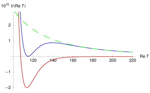
The minimum is lifted from AdS to dS, however the values for the moduli derived from the vacuum equations (5.127) do not significantly change during the uplift. Furthermore, the supersymmetry breaking parameters like the gravitino mass or soft–masses are essentially determined by the depth of the AdS–minimum and most of the soft–supersymmetry breaking pattern (exhibited in subsection 5.5) does apply.

The stability of AdS vacua in gravity coupled to scalar fields has been investigated in [494]. Stability is guaranteed, if all scalar masses fulfill the Breitenlohner–Freedman (BF) bound [494], i.e. their mass eigenvalues do not fall below a certain minimal bound. The latter is a negative number related to the scalar potential at the minimum (5.128). It can be shown in a completely model independent way that all scalars have masses above this bound at any ${\cal N}=1$ supersymmetric AdS minimum in supergravity theories. However, the third and final step in the KKLT scenario consists in the addition of one anti D3–brane, i.e. a positive contribution to the scalar potential, which lifts the AdS minimum to a dS minimum. The masses for the moduli fields do not change significantly during this process. However stable dS vacua require positive mass eigenvalues. Hence, any negative mass eigenvalue before the uplift is unacceptable since the effect of the anti D3–branes on the mass eigenvalues is too small to change a negative mass to positive.

The question under which conditions one may achieve a stable uplift from AdS to dS has been asked in [495, 347] (see also [496, 497, 498, 499, 500]) and further investigated in full generality in [340]. One important conclusion of the work [340] is, that compactifications without complex structure moduli, i.e. $h^{2,1}_{-}({\cal X})=0$ generically do not allow for a stable uplift. More precisely, there are certain constraints on the form of the Kähler potential for the Kähler moduli in order to yield positive mass eigenvalues. In particular, all $\mathbb{Z}_{N}$–and $\mathbb{Z}_{N}\times\mathbb{Z}_{M}$–orientifolds ${\cal X}$ with $h^{2,1}_{-}({\cal X})=0$ are excluded for a KKLT scenario. This concerns $\mathbb{Z}_{3},\mathbb{Z}_{7},\mathbb{Z}_{3}\times\mathbb{Z}_{3},\mathbb{Z}_{4}\times\mathbb{Z}_{4},\mathbb{Z}_{6}\times\mathbb{Z}_{6}$ and $\mathbb{Z}_{2}\times\mathbb{Z}_{6^{\prime}}$ –both at the orbifold point and away from it.

Finally we want to mention, that other scenarios for moduli stabilization and supersymmetry breaking in type IIB orientifolds have been developed in [501, 443, 497, 502]. Instead of the potential (5.129) the uplift from an AdS- to a dS-vacuum may be also achieved by a D-term potential (D–term uplift) [501]. However, it has been pointed out in [491] that a supersymmetric AdS minimum (5.127) cannot be uplifted by non–vanishing D–terms. On the other hand, in [497, 502] an appealing alternative has been proposed to break supersymmetry by F–terms $F_{\cal C}$ of open string moduli or matter fields (F–term uplift). In the matter dominated supersymmetry breaking scenario $F_{\cal M}\sim 0,\ F_{\cal C}\sim m_{3/2}$ supersymmetry is broken by non–vanishing F–terms of matter fields while essentially saving the stabilization results (5.127) of the closed string moduli furnished at the AdS minimum, c.f. [497, 502] for more details.

5.7 Type IIA flux compactifications

In order to explain the idea of flux compactifications we have focused on the prototype example of three-form fluxes in type IIB string theory. The main reason was that the backreaction of the fluxes on the geometry is under rather good control insofar as one deals with a conformal Calabi-Yau manifold as internal space. Neglecting the warp factor, one can employ the standard Calabi-Yau techniques and rely on the mathematical proofs for their existence.

Compared to type IIB, matters are more complicated in type IIA [416, 503, 504, 505, 506, 507, 508, 509, 510, 511, 512, 513, 207, 514]. In type IIA a similar analysis of the Killing spinor equations as sketched in section 5.2.2 leads to the conclusions that IIA solutions with non-vanishing NSNS or RR fluxes are either not symplectic or not complex, or neither. More concretely, a specific class of solutions of the type IIA Killing spinor equations is given by almost-Kähler, half-flat manifolds with the following torsion class

$$\tau\in{\cal W}_{2}^{+}\ .$$ (5.131)

It means that the holomorphic 3-form $\Omega_{3}$ is non-closed (cfr. eq.(5.2.2)):

$$d\Omega_{3}={\cal W}_{2}\wedge J_{2}\ .$$ (5.132)

This geometrical quantity can the be related to the non-vanishing RR fluxes in the following way:

$${\cal W}_{2}^{+}=e^{\phi}(F_{2}+F_{4})\ .$$ (5.133)

A similar analysis is actually true for flux compactifications with a four-dimensional AdS₄ space instead of Minkowski space-time [516]. Here the torsion is constrained to fall into the following classes:

$$\tau\in{\cal W}_{1}^{+}+{\cal W}_{2}^{+}\ .$$ (5.134)

Therefore the six-dimensional space is a half-flat manifold. In addition to 5.134, the Bianchi identities require the exterior derivate of ${\cal W}_{2}^{+}$ to be proportional to the real part of the (3,0)-form on the six-dimensional space:

$$d{\cal W}_{2}^{+}\sim{\rm Re}(\Omega)\ .$$ (5.135)

About the type IIA non-Calabi-Yau solutions to the supersymmetry constraints much less is known and examples are rare. To address the moduli problem one should first know the moduli space, which is not the case for these solutions. Nevertheless, one can try a perturbative approach and treat the fluxes and the backreaction of the metric and other fields as small effects. Effectively, one can then use the Calabi-Yau background and its moduli space. Let us sketch how one can proceed in type IIA in this way.

Type IIA theory contains the RR one-form $C_{1}$ and three-form $C_{3}$ as well as their Hodge dual forms $C_{7}$ and $C_{5}$. In addition, in type IIA Calabi-Yau orientifolds we have to deal with orientifold O6-planes that couple to the RR seven-form $C_{7}$ via (2.2.4), explicitly

$$Q_{6}\mu_{6}\int_{{\cal W}}C_{7}\ .$$ (5.136)

Regarding the effects of fluxes on the 6-brane charge one has to take care of a subtlety which was mentioned in the course of introducing the democratic type II action in section 2.2.3, namely the potential presence of RR field strengths without dynamical RR potentials. This includes the RR zero-form $F_{0}$ which is conventionally referred to as the mass parameter $m$ of IIA. Including this zero-form, the RR two-form field strength is defined

$$F_{2}=dC_{1}+F_{0}B_{2}\ .$$ (5.137)

By the democratic formulation, the equation of motion for $C_{7}$ is the Bianchi identity of $F_{2}$. Thus, the coupling (5.136) leads to a modification of this Bianchi identity in the presence of O6-planes in the form

$$dF_{2}=F_{0}H_{3}-Q_{6}\mu_{6}\pi_{3}\ .$$ (5.138)

Here $\pi_{3}$ is the Poincaré-dual three-form of the six-cycle wrapped by the O6-plane. Integrating this equation over any three-cycle produces a cancellation condition among the combination $F_{0}H_{3}$ of RR zero-form flux and NSNS three-form flux and the background O6-plane charge. Of course, adding D6-branes in addition would also contribute. This is the analogue of the effective three-brane charge (5.21) of three-form fluxes in IIB. Note that in IIA there are other RR fluxes which remain unconstrained.

The potential energy induced by the fluxes is obtained again by inserting a general ansatz for the fields into the action. All potentials are expanded into harmonic forms of proper degree on the Calabi-Yau. Fluxes are included for their field strengths. The dilaton is considered to be constant, and the metric a direct product of Minkowski times the Calabi-Yau. The kinetic action of the RR forms $F_{2p}$, $p=0,2,4$, is of course positive, and from the tension of the O6-planes there comes a negative contribution. This allows a stabilization with negative vacuum energy in a potentially supersymmetric AdS₄ groundstate.

The explicit dimensional reduction was performed in [148], where it was shown how to capture the effects of the fluxes in terms of a superpotential that has two pieces,

$$W_{\rm IIA-flux}={1\over\kappa_{10}^{2}}\,\int_{\cal X}\Big{[}\Omega_{3}\wedge H_{3}+\bigoplus_{p=0}^{3}F_{2p}\wedge e^{B+iJ_{2}}\Big{]}\ ,$$ (5.139)

which combines the general NSNS flux $H_{3}$ with the even RR fluxes $F_{2p}$. In addition, it is very plausible that the effective superpotential for type IIA compactifications on non-Calabi-Yau spaces contains a geometrical piece, which is determined by the non-vanishing torsion, i.e. the non-closure of $\Omega_{3}$, of the internal manifold (see also the similar expression for heterotic flux compactifications):

$$W_{\rm IIA-geometry}={1\over\kappa_{10}^{2}}\,\int_{\cal X}(d\Omega_{3}\wedge J_{2})\ .$$ (5.140)

The important difference compared to the case of IIB is the fact that (5.139) depends on both types of moduli, and thus complete moduli stabilization may in principle be achieved in IIA compactifications with fluxes [508, 509, 513, 517, 510, 511, 512, 207].

Now, the superpotential $W_{\rm IIA-flux}+W_{\rm IIA-geometry}$ is supposed to produce the correct conditions for preserving supersymmetry from its F-flatness. That means vanishing F-terms should impose the same constraints that follow from the Killing spinor equations. However this is quite difficult to be explicitly shown, since the moduli spaces of the non-Calabi Yau manifolds are not very well understood.

An alternative effective description was suggested basically based on experience with toroidal models and T-duality. The idea is that the deviation of the metric from being Calabi-Yau, i.e. the geometric torsion, could possibly be described by adding a background value for the spin connection $\omega_{ij}^{k}$, which can also be viewed as a three-index object. This has lead to the term “geometric flux”. Such geometric fluxes arise naturally from mirror symmetry to Type IIB flux compactifications and contribute both to the RR tadpole cancellation conditions as well as to the superpotential [416, 417]. They also give rise to new consistency conditions among fluxes and branes [511, 207]. The geometric fluxes deform the torus to a twisted torus. The resulting consistency conditions can be understood from their geometry and topology. In particular, it was pointed out that on the twisted torus the cohomology groups $H^{3}(\mathbb{T}^{6}_{\omega},\mathbb{Z})$ contain $\mathbb{Z}_{N}$ torsion pieces which give rise to extra tadpole cancellation conditions [455]. First attempts with concrete models with D6-branes and fluxes in IIA have been reported in [511, 518, 519, 520, 521]. From T-duality it was also conjectured that even more fluxes (or better flux-like deformations) could exist in so-called non-geometric compactifications [437].

Since in general type IIA flux vacua and other more general deformations of Calabi-Yau compactifications are not very well understood, we stop here.

5.8 Heterotic flux compactifications

Heterotic string compactifications on an internal space with non–trivial warp factor, dilaton and H–field background were first discussed in [42] (see also [140]. We will follow essentially the discussion in [503, 522]. More and also subsequent work on that subject can be found in [142, 523, 524, 525, 526, 527, 528, 529, 530, 531, 532, 533, 534, 535, 536, 537, 538, 539, 540, 541].

In the following, we will be interested in ${\cal N}=1$ supersymmetric compactifications of heterotic string theory on spaces with metric given by

$$ds^{2}=g^{0}_{MN}\,dx^{M}\otimes dx^{N}={\rm e}^{2\Delta(y)}\left(dx^{\mu}\otimes dx^{\nu}\,g_{\mu\nu}(x)+dy^{m}\otimes dy^{n}\,\hat{g}_{mn}(y)\right)\,.$$ (5.141)

Here ${g}_{\mu\nu}(x)$ denotes the metric of a four–dimensional maximally symmetric spacetime and $\Delta$ denotes a warp factor which we take to only depend on the internal coordinates $y^{m}$. The ten–dimensional supersymmetry equations (in the absence of gaugino condensates) can be cast into the following form

$$\delta\psi_{M} = {\cal D}_{M}\epsilon\equiv\nabla_{M}\epsilon-\frac{1}{4}H_{M}\epsilon\,,$$ (5.142)

$$\delta\chi = -\frac{1}{4}\,\Gamma^{MN}\epsilon\,F_{MN}\,,$$ (5.143)

$$\delta\lambda = -{1\over 4}\nabla\!\!\!\!/\phi+\frac{1}{24}\,H\,\epsilon\,,$$ (5.144)

where $H\equiv\Gamma^{MNP}H_{MNP}$, $H_{M}\equiv H_{MNP}\,\Gamma^{NP}$, and where the covariant derivative $\nabla$ is constructed from the rescaled metric $g_{MN}={\rm e}^{-2\phi}g_{MN}^{0}$. Necessary and sufficient conditions for ${\cal N}=1$ spacetime supersymmetry in four dimensions were derived in [42] and are given by:

1. the four–dimensional spacetime has to be Minkowski, i.e. ${g}_{\mu\nu}=\eta_{\mu\nu}$;

2. the internal six–dimensional manifold has to be complex, i.e. the Nijenhuis tensor $N_{mnp}$ has to vanish;

3. up to a constant factor, there is exactly one holomorphic $(3,0)$–form $\omega$, whose norm is related to the complex structure $J$ by

   $$\star d\star J=i\left(\bar{\partial}-\partial\right)\,\log||\omega||\,;$$ (5.145)

4. the Yang–Mills background field strength must be a $(1,1)$– form and must satisfy

   $$\hbox{tr}F\wedge F=\hbox{tr}\,\tilde{R}\wedge\tilde{R}-i\,\partial\bar{\partial}J\,$$ (5.146)

   as well as

   $$F_{mn}J^{mn}=0\,;$$ (5.147)

5. the warp factor $\Delta$ and the dilaton $\phi$ are determined by

   $$\Delta(y) = -{1\over 4}\phi(y)+{\rm constant}\;,$$

   $$\phi(y) = -\frac{1}{2}\log||\omega||+{\rm constant}\;;$$ (5.148)

6. the background three–form $H$ is determined in terms of $J$ by

   $$H=\frac{i}{2}\,\left(\bar{\partial}-\partial\right)J\,,$$ (5.149)

   where $i(\partial-{\bar{\partial}})=dx^{n}\,J_{n}\,^{m}\,\partial_{m}$.

Inspection of (5.146) shows that if ${\rm tr}\,{\tilde{R}}\wedge{\tilde{R}}$ is non–vanishing, then it has to be a $(2,2)$–form for consistency.

Next we will reformulate the conditions just mentioned in terms of torsional constraints, using the language of section 5.2.2. Since the internal manifold is taken to be complex, it immediately follows from that

$${\cal W}_{1}={\cal W}_{2}=0\,.$$ (5.150)

The torsion is therefore left in

$$\tau\in{\cal W}_{3}\oplus{\cal W}_{4}\oplus{\cal W}_{5}\,,$$ (5.151)

but it cannot be completely generic, because there is one further geometric constraint to be satisfied, namely (5.145). This equation relates the dual of the complex structure to the holomorphic (3,0)–form and therefore can be interpreted as a relation among the ${\cal W}_{4}$ and ${\cal W}_{5}$ classes. The ${\cal W}_{4}$ class is determined by $J\wedge dJ$ which, using the duality relation $\star J=\frac{1}{2}J\wedge J$, can be interpreted as $d\star J$. This implies that information about this class is encoded in the left–hand side of equation (5.145), as this is given by the one–form $\star d\star J$. Moreover, from the definition of ${\cal W}_{4}$, it follows that it must be described by a one–form, so it is interesting to establish the precise relation among the two quantities. We can rephrase the Hodge star dual and show that

$${\cal W}_{4}=\frac{1}{2}\,J\,\lrcorner\,dJ=\frac{1}{2}\,J\cdot\left(\star d\star J\right)\,.$$ (5.152)

The proof follows directly from the definition of the contraction operator

$$J\,\lrcorner\,dJ=\frac{3}{2}\;J^{sn}\;dx^{p}\;\nabla_{[s}J_{np]}=dx^{n}\;{J_{s}}^{p}\,\nabla_{p}{J_{n}}^{s}\,,$$ (5.153)

and of the Hodge dual:

$$J\cdot\left(\star d\star J\right)=-dx^{n}\;{J_{n}}^{s}\;\nabla_{p}{J_{s}}^{p}=dx^{n}\;{J_{s}}^{p}\;\nabla_{p}{J_{n}}^{s}\,.$$ (5.154)

Going back to (5.145), and in order to determine the precise relation between ${\cal W}_{4}$ and ${\cal W}_{5}$, we better consider multiplying (5.145) with $J$. In this way the equation gets simplified to

$${\cal W}_{4}=-\frac{1}{2}\,d\log||\omega||\,,$$ (5.155)

which gives a further constraint on ${\cal W}_{4}$, namely that it is an exact real 1–form. On the right hand side of this equation we find the norm of the holomorphic form, which is related to ${\cal W}_{5}$. Our classification of the torsion relies on the definition of a unit norm (3,0)–form, which in this case is simply

$$\Psi=\frac{\omega}{||\omega||}\,.$$ (5.156)

This form is not holomorphic anymore for a generic dilaton profile (which is then related to the $\omega$ norm) and that implies ${\cal W}_{5}\neq 0$. From the definition of the unit–norm (3,0)–form (5.156) it follows that

$$d\psi_{+}=\frac{1}{2}\,\left(d\Psi+d\bar{\Psi}\right)=-d\log||\omega||\wedge\psi_{+}\,.$$ (5.157)

The contraction with $\psi_{+}$ will therefore lead to

$${\cal W}_{5}=\frac{1}{2}\psi_{+}\,\lrcorner\,d\psi_{+}=d\log||\omega||\,,$$ (5.158)

and this finally translates into

$$2\,{\cal W}_{4}+{\cal W}_{5}=0\,.$$ (5.159)

With respect to concrete solutions of the above equations, it is possible to find manifolds that satisfy all these geometrical constraints. For instance the Iwasawa manifold is an explicit example for a solution of the geometrical heterotic supersymmetry conditions.. However there are additional constraints that are related to the heterotic Bianchi identities and to the equations in the heterotic gauge bundle sector. For non-Calabi Yau spaces with H-flux explicit constructions and solutions for heterotic gauge bundles are very hard to find. Hence we omit this part of the discussion and refer the reader to some of the relevant work in this direction [528, 539].

Now we want to discuss the effective action of heterotic flux compactifications. The aim is, like for type II flux compactifications, to find an effective superpotential $W_{het}$, which implements via $DW_{het}=0$ the same supersymmetry conditions that we have derived in the previous paragraph. The discussion will be still somewhat qualitative, since the moduli spaces of non-Calabi Yau manifolds are largely unknown. We start with the bosonic part of the Lagrangean up to second order in $\alpha^{\prime}$ is given by [542]

$$S = \int d^{10}x\,\sqrt{-g}\,e^{-2\phi}\left[\frac{1}{4}\,R-\frac{1}{12}H_{MNP}H^{MNP}+(\partial_{M}\phi)^{2}\right.$$ (5.160)

$$\qquad\qquad\qquad\;\;\left.-\frac{1}{4}\alpha^{\prime}\left(F_{MN}^{I}F^{I\,MN}-R^{+}_{MNPQ}R^{+\,MNPQ}\right)\,\right]\,.$$

This action is written in the string frame (we have set $\kappa_{10}^{2}=2$) and its fermionic completion makes it supersymmetric using the three–form Bianchi identity given by

$$dH=\alpha^{\prime}\left(\hbox{tr}\,R^{+}\wedge R^{+}-\hbox{tr}F\wedge F\right)\,,$$ (5.161)

where the curvature $R^{+}$ is the generalized Riemann curvature built from the generalized connection $\nabla^{+}$.

To simplify the discussion we limit ourselves to the case with dilaton and warp factor identified, i.e. $\phi=-4\Delta$, but the generalization of the following results is straightforward. After some manipulations, the action (5.160) can be written as

$$S= \int d^{4}x\,\sqrt{-g_{4}}\,\left\{-\frac{1}{2}\int_{{\cal X}}\,{\rm e}^{-2\phi}\left(-2d\phi+\theta\right)\wedge\star\left(-2d\phi+\theta\right)+\frac{1}{8}\int_{{\cal X}}{\rm e}^{-2\phi}\,J\wedge J\wedge{\hat{R}}^{ab}J_{ab}\right.$$ (5.162)

$$- \frac{1}{4}\int_{{\cal X}}d^{6}y\;\sqrt{g_{6}}\,{\rm e}^{-2\phi}\,N_{mn}{}^{p}\,g^{mq}g^{nr}g_{ps}\,N_{qr}{}^{s}\,$$

$$+ \frac{1}{2}\int_{{\cal X}}{\rm e}^{-2\phi}\,\left(H+\frac{1}{2}\star{\rm e}^{2\phi}\,d({\rm e}^{-2\phi}\,J)\right)\wedge\star\left(H+\frac{1}{2}\star{\rm e}^{-2\phi}\,d({\rm e}^{-2\phi}\,J)\right)\,$$

$$- \frac{\alpha^{\prime}}{2}\int_{{\cal X}}d^{6}y\;\sqrt{g_{6}}\,{\rm e}^{-2\phi}\,\left[\hbox{tr}(F^{(2,0)})^{2}+{\rm tr}(F^{(0,2)})^{2}+\frac{1}{4}\,\hbox{tr}(J^{mn}F_{mn})^{2}\right]$$

$$+ \left.\frac{\alpha^{\prime}}{2}\int_{{\cal X}}d^{6}y\;\sqrt{g_{6}}\,{\rm e}^{-2\phi}\,\left[\hbox{tr}(R^{+\,(2,0)})^{2}+\,\hbox{tr}(R^{+\,(0,2)})^{2}+\frac{1}{4}\,\hbox{tr}(J^{mn}R^{+}_{mn})^{2}\right]\right\}\,.$$

In this expression the traces are taken with respect to the fiber indices $a,b,\ldots$, whereas the Hodge type refers to the base indices $m,n,\ldots$ of the curvatures. The other geometrical objects appearing in the above expression are the Lee–form

$$\theta\equiv J\lrcorner dJ=\frac{3}{2}J^{mn}\,\partial_{[m}J_{np]}\,dx^{p}\,,$$ (5.163)

the Nijenhuis tensor

$$N_{mn}{}^{p}={J_{m}}^{q}\partial_{[q}J_{n]}{}^{p}-{J_{n}}^{q}\partial_{[q}J_{m]}{}^{p}\,,$$ (5.164)

and the generalized curvature $\hat{R}$, which is constructed using the Bismut connection built from the standard Levi–Civita connection and a totally antisymmetric torsion $T^{B}$ proportional to the complex structure,

$$T^{B}_{mnp}=\frac{3}{2}\,{J_{m}}^{q}{J_{n}}^{r}{J_{p}}^{s}\partial_{[q}J_{rs]}=-\frac{3}{2}J_{[m}{}^{q}\nabla_{|q|}J_{np]}\,.$$ (5.165)

The action (5.162) will now be used to find the conditions determining the background geometry. Namely, (5.162) can be used as the expression for the scalar potential of the effective four–dimensional theory,

$$S=-\int d^{4}x\,\sqrt{-g_{4}}\,{\cal V}\,.$$ (5.166)

The action (5.162) consists of a sum of squares as well as of one linear term. In order to have a solution of the equations of motion one sets to zero all the squares and proves that the linear term does not contribute to the equations of motion. First we would like to exhibit the correspondence between the supersymmetry conditions and the terms which are squared in the action. The geometrical conditions resulting from the vanishing of the BPS–like squares are the vanishing of the Nijenhuis tensor

$$N^{m}{}_{np}=0$$

and of some components of the generalized Riemann curvature constructed from the $\nabla^{+}$ connection,

$$R^{+\,(2,0)}=R^{+\,(0,2)}=J^{mn}R^{+}_{mn}=0.$$

The vanishing of the Nijenhuis tensor states that the internal manifold is complex (which means ${\cal W}_{1}={\cal W}_{2}=0$ in the torsion classes language). The conditions on the $R^{+}$ curvature can be translated into the integrability constraints following from the vanishing of the gravitino supersymmetry transformation (5.142), which leads to the requirement of $SU(3)$ holonomy for the $\nabla^{-}$ connection. The proof requires the identity

$$R^{+}_{ab\,cd}=R^{-}_{cd\,ab}-(dH)_{abcd}\,,$$ (5.167)

which relates the $R^{+}$ and $R^{-}$ curvatures with the base and fiber indices swapped. Using this identity and the fact that $dH$ gives higher order terms in $\alpha^{\prime}$ the conditions on the base indices of $R^{+}$ become conditions on the $R^{-}$ fiber indices, to lowest order in $\alpha^{\prime}$,

$$R^{-\,(2,0)}=R^{-\,(0,2)}=J^{ab}R^{-}_{ab}=0\,.$$ (5.168)

These conditions precisely state that the generalized curvature $R^{-}$ is in the adjoint representation of $SU(3)\subset SO(6)$ and therefore its holonomy group is contained in $SU(3)$. We also obtain the relation between the ${\cal W}_{4}$ and ${\cal W}_{5}$ torsion classes, expressed by the identification of the differential of the dilaton with the Lee–form,

$$d\phi-\frac{1}{2}\,\theta=0\,\,.$$ (5.169)

The final BPS–like square precisely yields the locking condition of the three–form $H$ onto the almost complex structure $J$ which was derived from the vanishing of the supersymmetry transformations. Indeed, on a complex manifold, and using (5.169), the following identity holds,

$$H=-\frac{1}{2}\star{\rm e}^{2\phi}\,d({\rm e}^{-2\phi}\,J)=\frac{1}{2}i(\partial-{\bar{\partial}})J\;.$$ (5.170)

Since the potential essentially consists of a sum of BPS–like squares, and is hence positive definite, we can derive it as a F-term potential from a holomorphic superpotential, plus various D–terms. The necessary requirements for having an ${\cal N}=1$ vacuum, i.e. $W=0$ and $\partial W=0$, then impose certain conditions leading to moduli stabilization. A rigorous derivation of the superpotential for flux compactifications requires a detailed knowledge of the moduli space of the compactification manifolds, which is not available at present. However an educated guess for the superpotential is given by [531, 522]

$$W_{het}={1\over 2}\int\Omega_{3}\wedge\left(H+\frac{i}{2}dJ\right)\,.$$ (5.171)

Notice that for generic flux compactifications the internal space is not complex, i.e. $J$ is not integrable, and therefore $dJ\wedge\Omega\neq 0$. Since the above superpotential explicitly depends on the three–form flux $H$, its extremisation should give rise to the torsional constraints leading to supersymmetric configurations. Again, a rigorous derivation requires an explicit knowledge of the metric moduli, but it is plausible that under certain assumptions the expected torsional constraints do follow. More precisely, the superpotential $W_{het}$ has to lead to a determination of $H$ in terms of the deviation of the internal space from being a Calabi–Yau manifold. $W_{het}$ must therefore also include pieces which are purely geometrical and which measure the non–Calabi–Yau–ness of the internal space. This is captured by the additional piece proportional to $dJ$ in (5.171).

Let us briefly comment on the limiting case with constant dilaton $\phi=const.$ and vanishing flux $H=0$. The locking condition (5.170) simply becomes the requirement for the internal manifold to be Kähler, imposing $dJ=0$. In addition, the square involving the dilaton becomes a condition imposing the vanishing of the Lee form, $d\star J=0$. Moreover, now $\nabla^{\pm}=\nabla$ and $R^{+}=R^{-}=R$. Therefore the conditions on the holonomy of $\nabla^{-}$ become conditions on the Levi–Civita connection. The solution is obviously given by Calabi–Yau manifolds, which are Kähler and have vanishing first Chern class.

6 STATISTICS OF FLUX AND D-BRANE MODELS

So far we have reviewed the various classes of string compactifications with ${\cal N}=1$ space-time supersymmetry in four dimensions. Both heterotic as well as D-brane constructions allow to realize many of the features for the SM, like gauge symmetry, chiral matter particles, gauge symmetry breaking, family replication etc. These discrete parameters are mostly of topological origin in string theory and are relatively well understood. When it comes to the continuous parameters like gauge or Yukawa couplings, string theory is far less under control, for first these terms in the effective action are only possible to be computed for simple toroidal orbifold models so far and second they depend sensitively on the moduli notoriously present in string compactifications.

However, as a big step forward it was realized that flux backgrounds (in addition to non-perturbative corrections) in general freezes these moduli either in supersymmetric or non-supersymmetric minima. However, with a method really determining (the classical or naked) energy density in a string vacuum, the so far neglected cosmological constant problem arises. In general one expects that quantum corrections generate a cosmological constant of the order of the supersymmetry breaking scale $M^{4}_{susy}=(1$TeV)⁴. In order to obtain the observed value of $\Lambda=(0.003$eV)⁴ a fine-tuning of the classical value is needed for which so far no physical reason has been identified.

As we will review in the next subsection, an estimate of the number of supersymmetric flux vacua in Type IIB orientifolds [543] comes to the conclusion that for general Calabi-Yau manifolds there exist of the order of $10^{500}$. This number dramatically exceeds most of the estimates for the number of string vacua made before. For instance the number of toric Calabi threefolds is 184026 [544]. An exception is the early estimate of the number of self-dual lattices in [13](see also [545]). Taking this number seriously, i.e. assuming that the number of vacua is not drastically reduced by taking non-perturbative corrections to the flux superpotential into account, led R. Bousso and J. Polchinski [546] to the proposal that the cosmological constant might not be fixed by a dynamical principle to such a small value but that this fine tuning is ”solved” by merely the enormous vacuum degeneracy of string vacua. Along this same line of reasoning, M.R. Douglas proposed that, complementary to a model by model search, one should follow a statistical approach to the string vacuum problem [547], as this large degeneracy seemed to make it very unlikely that we will easily identify models, which come close to our universe.

In [543, 548] very powerful statistical methods were developed to determine to distribution of Type IIB flux vacua over the complex structure moduli space. The generalization to M-theory flux vacua was performed in [549]. Since in this review we restrict ourselves to deal mainly with D-brane constructions, we do not review the entire story about the statistics in the flux sector. For short reviews on this subject we refer the reader to [550, 78] and for a more elaborate review to [75]. Here we mainly review the methods developed so far to describe the statistics in the D-brane sector. This should only be regarded as a first approach to the problem, as in a completely realistic setting the statistics of the D-brane sector has to be combined with the statistics of the flux sector.

6.1 Counting supersymmetric Type IIB flux vacua

In section 5 we have provided the formalism to describe flux vacua in Type IIB string theory. Just taking the tree level induced potential over the complex structure moduli space of a chosen Calabi-Yau manifold, one could ask the question

How many different flux vacua are there?

Following [548], let us make an estimate. Consider Type IIB compactified on a Calabi-Yau manifold with $b_{3}$ three-forms $\alpha^{i}$. Now we turn on general G-flux through these three-cycles

$${1\over\ell_{s}^{2}}H_{3}=\sum_{i}N^{i}_{NS}\,\alpha_{i},\quad\quad{1\over\ell_{s}^{2}}F_{3}=\sum_{i}N^{i}_{R}\,\alpha_{i},$$ (6.1)

so that

$$N_{\rm flux}={1\over\ell_{s}^{4}}\int F_{3}\wedge H_{3}=\eta_{ij}N^{i}_{NS}\,N^{j}_{R}>0$$ (6.2)

with $\eta_{ij}=\int\alpha_{i}\wedge\alpha_{j}$. The tadpole cancellation condition reads

$${N_{\rm flux}\over 2}+N_{D-branes}=L_{*}$$ (6.3)

where $L_{*}$ denotes the contribution of the orientifold planes. Now, we want to count the number of solutions with $0\leq L\leq L_{*}$ with $L=N_{\rm flux}/2$. This number is given by

$${\cal N}_{\rm flux}(L\leq L_{*}) = \sum_{{\rm susy\ vac}}\theta(L_{*}-L)$$

$$= \sum_{vac}{1\over 2\pi i}\int_{C}{d\alpha\over\alpha}e^{\alpha\,(L_{*}-L)}$$

$$= {1\over 2\pi i}\int_{C}{d\alpha\over\alpha}e^{\alpha\,L_{*}}\left(\sum_{vac}e^{-{\alpha\over 2}{\bf N}\,\eta\,{\bf N}}\right)$$

where the path $C$ in the complex plane runs parallel to the $y$ axis with small positive $x$. After approximating the discrete sum over the flux quanta by an integral, the sum over all vacua can be written as

$${\cal N}(\alpha) = \sum_{vac}e^{-{\alpha\over 2}{\bf N}\,\eta\,{\bf N}}$$ (6.5)

$$= \int_{M}d^{2m}z\int d^{4m}Ne^{-{\alpha\over 2}{\bf N}\,\eta\,{\bf N}}\,\delta^{2m}(DW)\,|\det D^{2}W|$$

with $m=b_{3}/2$ and $M$ denoting a fundamental region in the complex structure/dilaton moduli space. However, the scaling of the number of vacua with $L_{*}$ can be estimated without evaluating this integral. Let us rescale $N\to N/\sqrt{\alpha}$, which implies ${\cal N}(\alpha)\to\alpha^{-2m}{\cal N}(1)$ so that gets

$$N_{\rm flux}(L\leq L_{*}) = {1\over 2\pi i}\int_{C}{d\alpha\over\alpha^{2m+1}}e^{\alpha\,L_{*}}\,{\cal N}(1)$$ (6.6)

$$= \theta(L_{*})\,{L_{*}^{2m}\over(2m)!}\,{\cal N}(1).$$

This is good approximation as long as the radius of the sphere in $N$-space is large enough, i.e. $L_{*}\gg 2m$. For typical numbers such as $L_{*}\simeq 1000$ (as they appear in F-theory) and $m\simeq 200$ one gets ${\cal N}_{\rm flux}\simeq 10^{250}$. This is an amazingly large number, which is may orders of magnitudes larger than the ensembles of string vacua people have dealt with before, like for instance toric varieties [551], where numbers like $4\cdot 10^{9}$ occurred .

In [543] the integral (6.5) was evaluated further (with $|\det D^{2}W|$ $\to$ $\det D^{2}W$ ) leading eventually to the formula

$$N_{\rm flux}(L\leq L_{*}) = {2\pi L_{*}^{2m}\over\pi^{n}\,(2m)!}\,\int_{{\cal F}\times{\cal H}}\det\left(-R-\omega\right)$$ (6.7)

where ${\cal F}$ denotes the fundamental region of $SL(2,\mathbb{Z})$, ${\cal H}$ the fundamental region of the complex structure moduli space and $R$ and $\omega$ the curvature and Kähler two forms.

In view of this huge vacuum degeneracy, the so-called string landscape, M.R. Douglas has proposed a statistical approach to the string vacuum problem [547]. In its pragmatic version it says that complementary to a (necessary) model by model search one should study the statistical distribution of various physical quantities in the ensemble of string vacua. Such an approach might be helpful to

• estimate the frequency with which standard-like string models arise

• get an idea in which regions of the landscape to look for realistic models

• find statistical evidence that standard-like properties are extremely rare, i.e. almost excluded $\to$ falsification of string theory

• argue for a uniform distribution of certain physical quantities like for instance the cosmological constant, shedding a new light on so-called fine tuning problems

Our viewpoint is rather pragmatic stating that no final word has been spoken in this matter and one should carry on investigating the set of string vacua with all possible means. It might also be that without a completely understanding of M-theory we are missing some essential (non-perturbative) consistency conditions, which eventually will reduces the number of vacua.

6.2 Statistical approach for D-brane models

The statistics due to the closed string fluxes provide estimates for the frequency of cosmological parameters like the cosmological constant. Of course, for making contact with elementary particle physics and the SM, we have to also include the statistics of the open string sector in Type II orientifolds.

The statistics of D3-brane gauge groups in flux vacua has been investigated in [554]. A more general study of D-brane statistics was initiated in [555], where for the ensemble of intersecting branes on certain toroidal orientifolds, the statistical distribution of various gauge theoretic quantities was studied, like the rank of the gauge group, the number of models with an $SU(M)$ gauge factor and the number of generations. In particular, the examples of supersymmetric intersecting branes on the $T^{2}$, $T^{4}/\mathbb{Z}_{2}$ and $T^{6}/\mathbb{Z}_{2}\times\mathbb{Z}_{2}$ orientifolds were discussed in detail. These results were supplemented and confirmed by concrete results from a long term brute force computer search as reported in [556, 557, 558, 559]. In [560] the statistics of supersymmetric intersecting D-brane models on $T^{6}/\mathbb{Z}_{2}\times\mathbb{Z}_{2}$ orbifolds was also discussed. In contrast to [556, 557, 558, 559] here the distributions were discussed for fixed numbers of D-branes i.e. by neglecting the exponential degeneracy of the hidden sector branes. In particular it was proven that the number of tadpole canceling configurations is finite. Another example of models where a brute force statistical analysis was performed are the aforementioned Gepner model orientifolds [283, 287].

The models we are interested in are still supersymmetric intersecting D-brane models with the main constraints given by supersymmetry and the tadpole cancellation condition. The first step is to determine all or at least a large, preferably representative subset of supersymmetric branes. After solving the supersymmetry constraints, in all the examples discussed in [555], this was given by a subset $S$ of the naively allowed wrapping numbers $X_{I}$. As a constraint one faces the various tadpole cancellation conditions

$$\sum_{a=1}^{k}N_{a}\,X_{a,I}=L_{I}$$ (6.8)

with $I=1,\ldots,b_{3}/2$ and $L_{I}$ denoting the contribution from the orientifold planes and the three-form fluxes. A gauge theoretic quantity is often a function of the wrapping numbers and the number of D-branes. Therefore it is necessary to have methods to compute statistical distributions in the unconstrained set of solutions to (6.8).

6.2.1 Counting tadpole solutions

Let us discuss such a method at a very simple example, which however shows already the general idea. Say we would first count the solutions of the single tadpole condition

$$\sum_{a=1}^{k}N_{a}\,X_{a}=L.$$ (6.9)

By writing the Kronecker delta function as

$$\delta_{n,0}={1\over 2\pi i}\oint dq\,q^{n-1},$$ (6.10)

we can express this number as

$${\cal N}(L) \simeq {1\over 2\pi i}\oint dq{1\over q^{L+1}}\sum_{k=1}^{\infty}{1\over k!}\,\sum_{N_{1}=1}^{\infty}\sum_{X_{1}=1}^{L}\ldots\sum_{N_{k}=1}^{\infty}\sum_{X_{k}=1}^{L}q^{\sum_{a}N_{a}X_{a}}$$ (6.11)

$$= {1\over 2\pi i}\oint dq{1\over q^{L+1}}\sum_{k=1}^{\infty}{1\over k!}\,\left(\sum_{X=1}^{L}{q^{X}\over 1-q^{X}}\right)^{k}$$

A common method to evaluate the asymptotic expansion of such integrals is the saddle point approximation. First we write

$${\cal N}(L)={1\over 2\pi i}\oint{dq}\,e^{f(q)}.$$ (6.12)

To evaluate this integral one assumes that the main contribution comes from the saddle points $q_{0}$, which are determined by the condition $df/dq|_{q_{0}}=0$. Here we assume that there exists only one saddle point. Otherwise one has to sum over all saddle points. The leading order saddle point approximation is then simply given by

$${\cal N}^{(0)}(L)=e^{f(q_{0})}.$$ (6.13)

One can compute the next to leading order approximation

$${\cal N}^{(2)}(L)={1\over\sqrt{2\pi}}\,{e^{f(q_{0})}\over\sqrt{{\partial^{2}f\over\partial q^{2}}|_{q_{0}}}}.$$ (6.14)

In our case the saddle point function $f$ reads

$$f(q)=\sum_{X=1}^{L}{q^{X}\over 1-q^{X}}-(L+1)\,\log q.$$ (6.15)

Close to $q\simeq 1$ we find the analytical expression

$$f(q)\simeq{1\over 1-q}\sum_{X=1}^{L}{1\over X}-L\,\log q\simeq{\log L\over 1-q}-L\,\log q.$$ (6.16)

In this approximation the saddle point is at $q_{0}=1-\sqrt{\log L\over L}$ yielding the leading order approximation

$${\cal N}(L)\simeq e^{2\sqrt{L\log L}}.$$ (6.17)

A rough intuitive understanding of this result can be gained as follows: In order to solve (6.9) one first divides $L$ into its partitions and then one writes each term as a product of two positive integer numbers. We know already that the number of partitions scales like $e^{2\sqrt{L}}$. On the other hand it is known in number theory that the function $\sigma_{0}(n)$ of divisors of an integer $n$ has the property

$${1\over L}\sum_{n=1}^{L}\sigma_{0}(n)\simeq\log L+(2\gamma_{E}-1)$$ (6.18)

for $L>>1$, where $\gamma_{E}$ denotes the Euler-Mascheroni constant.

For the more general case of $b_{3}/2$ tadpole cancellation conditions, the number of such solutions is given by the expression

$${\cal N}(\vec{L}) \simeq {1\over(2\pi i)^{b_{3}\over 2}}\oint\prod_{I}{dq_{I}\over q_{I}^{L_{I}+1}}\,\exp\left(\sum_{X_{I}\in S}{\prod_{I}q_{I}^{X_{I}}\over 1-\prod_{I}q_{I}^{X_{I}}}\right),$$ (6.19)

which can be evaluated at leading order by a saddle point approximation with

$$f(\vec{q})=\sum_{X_{I}\in S}{\prod_{I}q_{I}^{X_{I}}\over 1-\prod_{I}q_{I}^{X_{I}}}-\sum_{I}(L_{I}+1)\,\log q_{I}.$$ (6.20)

The saddle point is determined by the condition $\nabla f(\vec{q})|_{\vec{q}_{0}}=0$, and the second order saddle point approximation reads

$${\cal N}^{(2)}(\vec{L})={1\over\sqrt{2\pi}^{b_{3}\over 2}}\,{e^{f(\vec{q}_{0})}\over\sqrt{\det\left[\left({\partial^{2}f\over\partial q_{i}\partial q_{j}}\right)\right]_{q_{0}}}}.$$ (6.21)

6.2.2 Distribution of physical quantities

We can also ask, what the percentage of models with at least one $SU(M)$ gauge factor is. Using the same methods as above this can be written

$$P(M) \simeq {1\over 2\pi i\,{\cal N(L)}}\oint dq\,{1\over q^{L+1}}\sum_{k=1}^{\infty}{1\over(k-1)!}\,\left(\sum_{X=1}^{L}{q^{X}\over 1-q^{X}}\right)^{k-1}\,\sum_{X=1}^{L}\sum_{N=1}^{\infty}q^{NX}\delta_{N,M}$$ (6.22)

$$= {1\over 2\pi i\,{\cal N(L)}}\oint dq\,{1\over q^{L+1}}\,\exp\left(\sum_{X=1}^{L}{q^{X}\over 1-q^{X}}\right)\,q^{M}\left({1-q^{ML}\over 1-q^{M}}\right)$$

The corresponding saddle point function reads

$$f(q)=\sum_{X=1}^{L}{q^{X}\over 1-q^{X}}+\log\left[q^{M}\left({1-q^{ML}\over 1-q^{M}}\right)\right]-(L+1)\,\log q.$$ (6.23)

We can either numerically search for saddle points of this function or we can observe that for $M\ll L$ the second, $M$ dependent, term in (6.23) is just a small perturbation. In this case we expect that in leading order the saddle point does not change, so that we have only to evaluate (6.23) at $q_{0}=1-\sqrt{L\log L}$. Doing this for large $L$ one expects that the probability to find an $SU(M)$ gauge factor scales like

$$P(M)\simeq\exp\left(-\sqrt{\log L\over L}M\right).$$ (6.24)

In Figure 20 we have shown the frequency for at least one $SU(M)$ factor for L=25.

Figure 20: Frequency of at least one $SU(M)$ factor for L=25. The dots show the exact results and the curve the saddle point approximation.

We see that the exact and saddle point approximation nicely agree in the regime $M\ll L$ and that for $M\simeq L$ we get deviations from the simple (6.24) behavior.

Next we investigate what the frequency is to get a gauge group of total rank $r$. This means that we also have to implement the constraint

$$\sum_{a}N_{a}=r,$$ (6.25)

which we again do by writing the Kronecker delta function as a contour integral

$$P(r) \simeq {1\over 2\pi i\,{\cal N}(L)}\oint dq{1\over q^{L+1}}\oint dz{1\over z^{r+1}}\sum_{k=1}^{\infty}{1\over k!}\,\sum_{N_{1}=1}^{\infty}\sum_{X_{1}=1}^{L}\ldots\sum_{N_{k}=1}^{\infty}\sum_{X_{k}=1}^{L}q^{\sum_{a}N_{a}X_{a}}\,z^{\sum_{a}N_{a}}$$ (6.26)

$$= {1\over 2\pi i{\cal N}(L)}\oint dq{1\over q^{L+1}}\oint dz{1\over z^{r+1}}\exp\left(\sum_{X=1}^{L}{z\,q^{X}\over 1-z\,q^{X}}\right).$$

Then the saddle point function reads

$$f(q,z)=\sum_{X=1}^{L}{z\,q^{X}\over 1-z\,q^{X}}-(L+1)\,\log q-(r+1)\,\log z.$$ (6.27)

Numerically determining the saddle point now in the two variables, $q$ and $z$ we find the Gaussian like distribution shown in Figure 21.

Figure 21: The rank distribution for $L=16$. The dots show the exact results and the curve the saddle point approximation.

After having checked in [555] that the number of solutions to the tadpole cancellation conditions for fixed complex structures for the 8D, 6D and 4D examples are finite, various gauge theoretic distributions were computed and compared to a brute force computer classification. Cutting a long story short, the following qualitative results we obtained

• The frequency to find an $SU(M)$ gauge factor scales like

  $$P(M)\simeq\exp\left(-\sqrt{\log L\over L}M\right).$$ (6.28)

  For a product gauge group $\prod_{i=1}^{k}SU(M_{i})$ with $\sum_{i=1}^{k}M_{i}\ll L$ it satisfies mutual independence, i.e. $P(M_{1}\,\ldots M_{k})=\prod_{i}P(M_{i})$.

• The rank distribution yields approximately a Gauss curve with the maximum depending on the complex structure moduli.

• Defining a measure for the chirality of a solution by $\chi=\langle\Pi^{\prime}\circ\Pi\rangle$, in the 6D case a dependence like

  $$P(\chi)\simeq\exp\left(-\kappa\,\sqrt{\chi}\right)$$ (6.29)

  was found with $\kappa$ denoting some constant depending presumably on the $L_{I}$.

6.2.3 Statistical correlations

An important question is whether one can see any statistical correlations of physical quantities. Here one can distinguish two kinds of correlations:

• Correlations which are directly the effect of the stringy consistency conditions like for instance the tadpole cancellation conditions. Though rather obvious from the stringy point of view, from a pure field theoretical or mathematical point of view, these correlations may nevertheless be quite surprising. A good example of such a correlation is for instance mirror symmetry, which is rather trivial from the world-sheet point of view, but rather surprising from the target space point of view.

• Correlations which are not obvious at all and cannot easily be traced back to the defining string equations.

All correlations known so far are of the first type. In the ensemble of intersecting D-brane models one finds for instance a correlation between the rank of the gauge group (6.25) and the mean chirality of the model (see figure 22), which we have defined as

$$\chi=<\Pi_{a}^{\prime}\circ\Pi_{b}-\Pi_{a}\circ\Pi_{b}>.$$ (6.30)

Figure 22: The frequency rank distribution of models of specific rank and chirality. $L_{0}=L_{1}=L_{2}=L_{3}=8$ and complex structures $U_{I}=1$.

This correlation was anticipated in [555] employing the saddle point approximation and confirmed in [556] by a direct computer search. It roughly speaking says that the higher the rank of the total gauge symmetry is the smaller is the number of generations in the model.

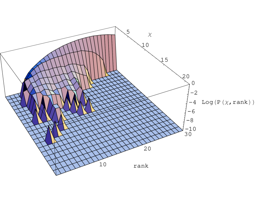
6.2.4 Statistical distributions of gauge theoretic quantities

In view of phenomenological applications of intersecting D-brane models it is interesting to learn something about the frequency of MSSM like models in this framework. In [556] of the order of $10^{8}$ intersecting D-brane models have been constructed, for which various statistical distributions were plotted. The main emphasis was on the statistics of semi-realistic models containing a subset of D-branes realizing the Standard Model quiver or a variation thereof. It was exemplified that most of the Standard Model features can be considered as being statistically independent, which allowed one to make an estimate for the frequency of MSSM-like models in this set-up. The individual suppression factors are listed in Table 29.

Restriction	Factor
gauge factor $U(3)$	$8.16\cdot 10^{-2}$
gauge factor $U(2)/SP(2)$	$9.92\cdot 10^{-1}$
No symmetric representations	$8.39\cdot 10^{-1}$
Massless $U(1)$	$4.23\cdot 10^{-1}$
Three generations of quarks	$2.92\cdot 10^{-5}$
Three generations of leptons	$1.62\cdot 10^{-3}$
Total	$1.3\cdot 10^{-9}$

Table 29: Suppression factors for various constraints of Standard Model properties.

Combining all these factors leads to an overall suppression factor of $\approx\,1.3\cdot 10^{-9}$. For plots of other statistical distributions we refer the reader to the original paper [556].

6.3 Outlook on statistics

Clearly, we are just beginning to approach the problem of unraveling the statistics on the landscape of string theory. The final aim would be to perform the statistics over as many parameters as possible to really get a realistic picture of what overall statistical averages can tell us about the distribution of various physical quantities. The methods shown above might play an important role whenever one encounters string theoretic constraints similar to the tadpole cancellation conditions. More modestly, as a next step it would be interesting to study the distributions of heterotic string vacua and to see whether, as expected from string dualities, they feature similar patterns as the orientifolds . Gepner model orientifolds [284, 287] might also provide a nice testing ground for comparing and possibly refining the technical statistical tools.

In principle, having agreed upon a good statistical ensemble one would like to address questions concerned directly with the Standard Model, like:

• What is the percentage of models having the right gauge group, matter and number of families?

• How drastically is this number reduced by requiring more detailed constraints, like the correct gauge and Yukawa couplings, the right Higgs couplings, absence of exotic matter?

• Having installed all phenomenological constraints, how does the distribution of the supersymmetry breaking scale and the cosmological constant look like?

The answers to these questions will strongly depend on possible statistical correlations among the various quantities.

Finally, let us mention that the idea of a stringy landscape has also influenced the way people think about other fine tuning problems, like for instance the gauge hierarchy problem. This has led to the idea of split supersymmetry [238], which still gives rise to gauge coupling unification at the GUT scale but does not employ low energy supersymmetry for stabilizing the weak scale.

7 CONCLUSIONS

Let us close with a summary of the status of the attempts we have covered here to find a realistic string vacuum. We find it fair to say that despite the enormous effort and the unquestionable successes in understanding the structure of string models so far there is no fully realistic candidate. We have discussed models with essential features of the Standard Model, but all promising candidates fail to be realistic at a certain step. In the end, a successful string compactification would need to solve the moduli problem explicitly and make all parameters computable which is still beyond our capabilities. Before getting desperate about this situation one should keep in mind, though, that we are only looking in very special corners of the overall configuration space, namely those which are technically accessible and under good control. Toroidal orbifolds are the most computable examples, Gepner models or geometric compactification at large radius defined by vector bundles on Calabi-Yau manifolds are alternatives. For most other string compactifications we cannot even answer the most elementary questions.

Therefore, a scan of all possible string vacua is far beyond our understanding and computational abilities. As argued in [563] the complexity of the task to identify the physically relevant vacua among the set of all vacua may fall in the category of so-called NP-hard problems. This may be a reason why we have not found the completely successful model yet. So far, we can only see the tip of the iceberg. The search for a realistic vacuum is unquestionably one of the most essential tasks in string theory, arguably the most ambitious computational problem ever encountered in theoretical physics. The reputation of string theorists will have to be measured by the answer delivered to this question.

In this review article we have collected a number of technical tools usable for building models describing various classes of ${\cal N}=1$ supersymmetric four-dimensional string compactifications. There are techniques applicable in the geometric large radius regime and conformal field theory methods which can be used for certain special points in the parameter space. A better understanding of the physics in the intermediate regime would be highly desirable. It would be of great impact to obtain concrete information on superpotentials, both classical contributions and those generated by world-sheet or space-time instantons. The way these can lift part of the moduli space is still not well understood. In order to really quantitatively relate string compactifications to low energy physics higher order corrections in perturbation theory are equally important. This refers in particular to the Kähler potential. A numerical approach along the line proposed in [564] might turn out to be promising.

The problem of moduli stabilization needs to find a solution before any string compactification can lead to fully a determined effective Lagrangian. It is also at the heart of the naturalness problems of standard field theory. In this sense, without a fully satisfactory moduli stabilization, there are no completely realistic string compactifications anyways. We have here also partly reviewed the mechanism of moduli stabilization through fluxes or similar deformations of Calabi-Yau compactifications in type II string theories. It provides a simple and, at least in cases, controllable way to stabilize part of the moduli scalars. This subject is currently still debated very actively and final conclusions are hard to identify yet. The general set of fluxes permissable in a given model, the consistency conditions that have to be satisfied when D-branes are present as well, and a number of conceptual issues such as the proper treatment of backreaction are examples for open questions that bear some impact on the models one can construct. It is not finally excluded that quantum physics of fluxes in string theory could spoil some of the results obtained in the classical approach mostly used at present.

On the other hand, taking the known formulas for potentials induced by fluxes seriously leads unavoidably to the enormous proliferation in the number of string vacua. This would change the nature of the vacuum problem significantly. It would provide at least a logical rationale for a statistical solution of the naturalness problems, the gauge hierarchy of the Standard Model and the cosmological constant problem, but at the prize of sacrificing the strict predictability of the theory. Statistical methods might then become really mandatory to get any insight into the distributions of physical quantities. This would, of course, leave many problems. It would be hard or impossible to decide which parameters have statistical or environmental explanations and which ones are uniquely determined and predictable by the dynamics of the theory. A simple example where both possibilities could in principle apply is the question why the space we live in has four macroscopic space-time dimensions.

Regarding this issue, we do not expect to be any close to an answer. We know far too little about the structure of string theory and its space of solutions. Within the available experimental and theoretical understanding of nature none of the two possibilities is excluded, there may exist a multiverse and part of the physics in our own universe is explained environmentally, or maybe a better understanding of full quantum M-theory could tell us the dynamical selection principle for four dimensions. Research remains a historical process, and time will tell.

Acknowledgements

R.B. and D.L. would like to thank the KITP Santa Barbara and St.St. CERN for hospitality. R.B. also thanks Rutgers University, where part of this review was written.

We would like to thank all our collaborators for working with us during the last six years on the material presented in this article: C. Angelantonj, K. Behrndt, M. Berg, V. Braun, J. Conlon, M. Cvetič, G. Curio, G. Dall’Agata, F. Epple, M. Gaberdiel, F. Gmeiner, L. Görlich, M. Haack, R. Helling, G. Honecker, A. Klemm, A. Krause, D. Krefl, P. Langacker, G. Lopes Cardoso, P. Manousselis, F. Marchesano, P. Mayr, S. Moster, P. Nath, T. Ott, E. Plauschinn, S. Reffert, R. Richter, E. Scheidegger, W. Schulgin, G. Shiu, K. Suruliz, T.R. Taylor, S. Theisen, P.K. Tripathy, D. Tsimpis, A. Van Proeyen, T. Weigand, M. Zagermann and G. Zoupanos.

Moreover, over the years we have learnt very much from interesting discussions with B. Acharya, N. Akerblom, G. Aldazabal, M. Alim, S. de Alwis, I. Antoniadis, R. Apreda, C. Bachas, K. Becker, M. Becker, M. Bianchi, D. Cremades, F. Denef, J.-P. Derendinger, K. Dienes, M. Douglas, E. Dudas, G. Dvali, J. Erdmenger, M. Faux, A. Faraggi, S. Ferrara, B. Florea, S. Förste, A. Font, M. Graña, T. Grimm, Y.H. He, A. Hebecker, L. Ibáñez, C. Jeschek, H. Jockers, S. Kachru, R. Kallosh, E. Kiritsis, S. Körs, C. Kounnas, W. Lerche, A. Linde, J. Louis, A. Lukas, A. Miemiec, H.P. Nilles, B. Ovrut, F. Quevedo, G. Pradisi, R. Rabadan, M. Ratz, R. Reinbacher, A. Sagnotti, B. Schellekens, M. Schmidt-Sommerfeld, C. Sieg, E. Silverstein, M. Trigiante, A. Uranga and F. Zwirner.

This work is supported in part by the European Community’s Human Potential Programme under contract MRTN-CT-2004-005104 ‘Constituents, fundamental forces and symmetries of the universe’.

Appendix A Some basics of CFT

We collect some basic formulas for the world sheet CFT of the superstring, sticking to the conventions of [61, 62].

A.1 Free closed string CFT

The world sheet sigma-model for a ten-dimensional flat target space with free scalars and fermions in super conformal gauge is

$${\cal S}=\frac{1}{2\pi\alpha^{\prime}}\int_{\Sigma}d^{2}z\,\Big{[}\partial X^{M}\bar{\partial}X_{M}+\frac{\alpha^{\prime}}{2}\Big{(}\psi^{M}\bar{\partial}\psi_{M}+\tilde{\psi}^{M}\partial\tilde{\psi}_{M}\Big{)}\Big{]}\ .$$ (A.1)

It is obtained from the general closed string sigma-model (2.1.1) by specifying to a target space with $G_{MN}=\eta_{MN},\,B_{MN}=0,$ and constant $e^{\Phi}=g_{s}$. The gauge field at the boundary is set to zero, $A_{M}=0$. The complex world sheet coordinates are defined

$$z=\exp(-i\sigma_{1}+\sigma_{2})\ .$$ (A.2)

The equations of motion are

$$\partial\bar{\partial}X^{M}(z,\bar{z})=0\ ,\quad\partial\tilde{\psi}^{M}(z,\bar{z})=\bar{\partial}\psi^{M}(z,\bar{z})=0\ .$$ (A.3)

Periodicity condition are imposed by $\sigma_{1}\equiv{\sigma}_{1}+2\pi$, while $-\infty<\sigma_{2}<\infty$. They are

$$X^{M}(\sigma_{1},\sigma_{2})~{}=~{}X^{M}(\sigma_{1}+2\pi,\sigma_{2})\ ,$$ (A.4)

$$\psi^{M}(\sigma_{1},\sigma_{2})~{}=~{}e^{2\pi i\nu}\psi^{M}(\sigma_{1}+2\pi,\sigma_{2})\ ,\quad\tilde{\psi}^{M}(\sigma_{1},\sigma_{2})~{}=~{}e^{2\pi i\tilde{\nu}}\tilde{\psi}^{M}(\sigma_{1}+2\pi,\sigma_{2})\ ,$$

the signs referring to the periodic Ramond ($\nu,\tilde{\nu}=0$) or the anti-periodic Neveu-Schwarz ($\nu,\tilde{\nu}=\frac{1}{2}$) sectors. Periodicities for left- and right-moving fermions can be chosen independently, giving rise to four different sectors, RR, NSNS, RNS, and NSR. One can now split the fields into holomorphic left- and anti-holomorphic right-movers, $X^{M}=X^{M}_{L}(z)+X^{M}_{R}(\bar{z})$, $\psi^{M}=\psi^{M}(z)$, $\tilde{\psi}^{M}=\tilde{\psi}^{M}(\bar{z})$, with

$$X^{M}_{L}(z) = \frac{x^{M}}{2}-i\frac{\alpha^{\prime}}{2}p_{L}^{M}\ln(z)+i\sqrt{\frac{\alpha^{\prime}}{2}}\sum_{n\neq 0}\frac{\alpha_{n}^{M}}{n}z^{-n}\ ,$$

$$X^{M}_{R}(\bar{z}) = \frac{x^{M}}{2}-i\frac{\alpha^{\prime}}{2}p_{R}^{M}\ln(\bar{z})+i\sqrt{\frac{\alpha^{\prime}}{2}}\sum_{n\neq 0}\frac{\tilde{\alpha}_{n}^{M}}{n}\bar{z}^{-n}\ ,$$

$$\psi^{M}(z) = \sum_{r\in\mathbb{Z}+\nu}\psi_{r}^{M}z^{-r-1/2}\ ,$$

$$\tilde{\psi}^{M}(\bar{z}) = \sum_{r\in\mathbb{Z}+\tilde{\nu}}\tilde{\psi}_{r}^{M}\bar{z}^{-r-1/2}\ .$$ (A.5)

The total momentum and winding is defined

$$p^{M}=\frac{1}{2}\Big{(}p^{M}_{L}+p^{M}_{R}\Big{)}\ ,\quad w^{M}=\frac{1}{2}\Big{(}p^{M}_{L}-p^{M}_{R}\Big{)}\ .$$ (A.6)

The algebra of raising and lowering operators is

$$[\alpha^{M}_{n},\alpha^{N}_{m}] = [\tilde{\alpha}^{M}_{n},\tilde{\alpha}^{N}_{m}]~{}=~{}n\delta_{n,-m}\eta^{MN}\ ,$$

$$\{\psi^{M}_{r},\psi^{N}_{s}\} = \{\tilde{\psi}^{M}_{r},\tilde{\psi}^{N}_{s}\}~{}=~{}\delta_{r,-s}\eta^{MN}\ ,$$

$$\big{[}x^{M},p^{N}\big{]} = i\eta^{MN}\ .$$ (A.7)

The closed string Hamiltonian is given by

$${\cal H}_{\rm cl}=L_{0}+\bar{L}_{0}\ ,$$ (A.8)

with

$$L_{0}=\frac{\alpha^{\prime}}{4}p_{L}^{2}+\frac{1}{2}\sum_{n\neq 0}\alpha^{M}_{-n}\alpha_{Mn}+\frac{1}{2}\sum_{r\in\mathbb{Z}+\nu}r\psi^{M}_{-r}\psi_{Mr}+a\ ,$$ (A.9)

and similarly $\bar{L}_{0}$ for the right-movers. The normal ordering constant $a$ takes values $\frac{1}{24}$ for each real periodic fermion, and $-\frac{1}{48}$ for antiperiodic fermions, and opposite signs for bosons. Thus, in flat Minkowski space-time it is $a=0$ in a R and $a=-\frac{1}{2}$ in NS sectors. The world sheet fermion number operators are

$$F=\sum_{r\in\mathbb{Z}+\nu}\psi^{M}_{-r}\psi_{Mr}\ ,\quad\tilde{F}=\sum_{r\in\mathbb{Z}+\tilde{\nu}}\tilde{\psi}^{M}_{-r}\tilde{\psi}_{Mr}\ .$$ (A.10)

A.2 Free closed strings with boundaries

One may now impose boundary conditions e.g. at ${\sigma}_{2}=0$, i.e. on the unit circle $z=1/\bar{z}$. For the bosons Neumann boundary conditions are $\partial_{{\sigma}_{2}}X^{M}=0$, Dirichlet conditions $\partial_{{\sigma}_{1}}X^{M}=0$. For the bosonic modes this translates into

$${\rm N:} \quad p^{M}=0\ ,\quad\alpha^{M}_{n}+\tilde{\alpha}_{-n}^{M}=0\ ,$$

$${\rm D:} \quad w^{M}=0\ ,\quad\alpha^{M}_{n}-\tilde{\alpha}_{-n}^{M}=0\ .$$ (A.11)

The mode expansion that satisfy the boundary conditions are

$${\rm N:} \quad X^{M}(z,\bar{z})=x^{M}-i\frac{\alpha^{\prime}}{2}w^{M}\ln(z{\bar{z}})+i\sqrt{\frac{\alpha^{\prime}}{2}}\sum_{n\neq 0}\frac{\alpha_{n}^{M}}{n}\bigg{[}\frac{1}{z^{n}}+\frac{1}{\bar{z}^{n}}\bigg{]}\ ,$$

$${\rm D:} \quad X^{M}(z,\bar{z})=x^{M}-i\frac{\alpha^{\prime}}{2}p^{M}\ln(z\bar{z})+i\sqrt{\frac{\alpha^{\prime}}{2}}\sum_{n\neq 0}\frac{\alpha_{n}^{M}}{n}\bigg{[}\frac{1}{z^{n}}-\frac{1}{\bar{z}^{n}}\Big{]}\ .$$ (A.12)

By forming linear combinations more general boundary conditions (2.9) can be imposed for constant $G_{MN}$ and ${\cal F}_{MN}$. The mode expansions are also just superpositions of the free fields.

The boundary conditions for the fermionic coordinates leave a freedom of choice for the spin structure at the boundary [91]. This is is reflected in the value of $\eta=\pm 1$ in

$${\rm N:}\quad\psi^{M}+i\eta\tilde{\psi}^{M}=0\Big{|}_{\partial{\Sigma}}\ ,\quad{\rm D:}\quad\psi^{M}-i\eta\tilde{\psi}^{M}=0\Big{|}_{\partial{\Sigma}}\ .$$ (A.13)

Mode expansions are easily constructed from (A.1).

A.3 Free open string CFT

The open string is defined by supplementing (A.1) and (A.3) with boundary conditions at ${\sigma}_{1}=0,\pi$, the real axis $z=\bar{z}$, while $0\leq{\sigma}_{1}\leq\pi$ and $-\infty<{\sigma}_{2}<\infty$. Neumann conditions read $\partial_{{\sigma}_{1}}X^{M}=0$ and Dirichlet $\partial_{{\sigma}_{2}}X^{M}=0$, opposite from the condition for the closed string imposed at fixed ${\sigma}_{2}$. The mode expansion of the open string reads

$${\rm N:} \quad X^{M}(z,\bar{z})=x^{M}-i\alpha^{\prime}p^{M}\ln(z\bar{z})+i\sqrt{\frac{\alpha^{\prime}}{2}}\sum_{n\neq 0}\frac{\alpha_{n}^{M}}{n}\Big{[}\frac{1}{z^{n}}-\frac{1}{\bar{z}^{n}}\Big{]}\ ,$$

$${\rm D:} \quad X^{M}(z,\bar{z})=x^{M}-i\alpha^{\prime}w^{M}\ln(z\bar{z})+i\sqrt{\frac{\alpha^{\prime}}{2}}\sum_{n\neq 0}\frac{\alpha_{n}^{M}}{n}\Big{[}\frac{1}{z^{n}}+\frac{1}{\bar{z}^{n}}\Big{]}\ .$$ (A.14)

The normalization of the space-time momentum $p^{M}$ and the winding $w^{M}$ differs by a factor 2 compared to (A.2). At the boundary there is again a choice of spin structure for the fermions. By the “doubling trick” one defines $\psi^{M}({\sigma}_{1},{\sigma}_{2})$ for ${\sigma}_{1}\in[0,2\pi]$ via $\psi^{M}({\sigma}_{1},{\sigma}_{2})=\tilde{\psi}(2\pi-{\sigma}_{1},{\sigma}_{2})$ for ${\sigma}_{1}\in[\pi,2\pi]$. With this construction the open string fermion behaves in all respect like a single holomorphic fermion with either periodic or anti-periodic periodicity, i.e. with a R and an NS sector. The periodicity of the fields also depends ont he types of boundary conditions at both ends, NN or DD leading to periodic R and antiperiodic NS fields, and vice vers for ND or DN boundary conditions.

The algebra of the open string mode operators is then also just the holomorphic part of (A.1) and the open string Hamiltonian is

$${\cal H}_{\rm op}=L_{0}={\alpha}^{\prime}p^{2}+\frac{1}{2}\sum_{n\neq 0}{\alpha}^{M}_{-n}{\alpha}_{Mn}+\frac{1}{2}\sum_{r\in\mathbb{Z}+\nu}r{\psi}^{M}_{-r}{\psi}_{Mr}+a\ .$$ (A.15)

The normal ordering constant $a$ depends on the periodicity of the fields just as for the closed string sectors.

A.4 Free CFT of intersecting branes

It is straightforward to generalize the above to the situation of closed and open strings that end on D-branes that are rotated and intersecting. Consider for simplicity the boundary conditions (2.209) in a two-dimensional plane or on a two-dimensional torus. It is useful to introduce complex coordinates

$$Z=X^{1}+UX^{2}\ ,\quad\bar{Z}=X^{1}+\bar{U}X^{2}\ ,\quad{\Psi}={\psi}^{1}+U{\psi}^{2}\ ,\quad\bar{\Psi}={\psi}^{1}+\bar{U}{\psi}^{2}\ ,$$ (A.16)

where $U$ can be the complex structure of the torus. Let us simplify by setting $U=i$. The mode operators are similarly complexified, e.g. ${\alpha}_{n}={\alpha}^{1}_{n}+i{\alpha}^{2}_{n}$, $\bar{\alpha}_{n}={\alpha}^{1}_{n}-i{\alpha}^{2}_{n}$, $\tilde{\alpha}_{n}=\tilde{\alpha}^{1}_{n}+i\tilde{\alpha}^{2}_{n}$, $\tilde{\bar{\alpha}}_{n}=\tilde{\bar{\alpha}}^{1}_{n}+i\tilde{\bar{\alpha}}^{2}_{n}$, and so on.

Boundary conditions for a one-dimensionally extended D-brane along the plane, rotated by an angle ${\varphi}$, can be written

$$\partial_{{\sigma}_{1}}{\rm Re}(e^{i{\varphi}}Z)=0\Big{|}_{\partial{\Sigma}}\ ,\quad\partial_{{\sigma}_{2}}{\rm Im}(e^{i{\varphi}}Z)=0\Big{|}_{\partial{\Sigma}}\ .$$ (A.17)

It is again straightforward to write the linear combinations of mode expansions that satisfy these boundary conditions. An alternative formulation is the rotated boundary state that satisfies the closed string boundary conditions above. Starting from (2.25) one only has to apply a rotation to a state with ND boundary conditions. One gets

$$|B,{\varphi},\eta\rangle_{\rm osc} = \exp\Big{(}-\frac{1}{2}\sum_{n>0}\frac{1}{n}(e^{2i{\varphi}}{\alpha}_{-n}\tilde{\alpha}_{-n}+e^{-2i{\varphi}}\bar{\alpha}_{-n}\tilde{\bar{\alpha}}_{-n})$$

$$\hskip 56.9055pt-\frac{i}{2}\eta\sum_{r>0}(e^{2i{\varphi}}{\psi}_{-r}\tilde{\psi}_{-r}+e^{-2i{\varphi}}\bar{\psi}_{-r}\tilde{\bar{\psi}}_{-r})\Big{)}|B,\eta,0\rangle_{\rm osc}\ .$$

Note that this describes only the oscillator part of the full boundary state, its zero mode pieces will also change under the rotation. From here one can read off that in the annulus tree channel amplitude, the overlap of two such states with potentially different rotation angles, a phase factor appears.

Open strings with rotated boundary conditions can best be described by their mode expansions. As long as the boundary conditions at the two ends ${\sigma}_{1}=0,\pi$ are identical (the two rotation angles equal) the solutions are again obtained by simple rotation from (A.3). When the open strings stretch between two sets of branes that are rotated at different relative angles, they have to satisfy

$$\partial_{{\sigma}_{2}}{\rm Re}(e^{i{\varphi}_{a}}Z)=0\Big{|}_{{\sigma}_{1}=0}\ ,\quad\partial_{{\sigma}_{1}}{\rm Im}(e^{i{\varphi}_{a}}Z)=0\Big{|}_{{\sigma}_{1}=0}\ ,$$

$$\partial_{{\sigma}_{2}}{\rm Re}(e^{i{\varphi}_{b}}Z)=0\Big{|}_{{\sigma}_{1}=\pi}\ ,\quad\partial_{{\sigma}_{1}}{\rm Im}(e^{i{\varphi}_{b}}Z)=0\Big{|}_{{\sigma}_{1}=\pi}\ .$$ (A.19)

Fields are no longer periodic or anti-periodic, and modes are not integer or half-integer. Instead, the mode levels are shifted in the form $n\in\mathbb{Z}\pm{\delta}_{ab}$ and $r\in\mathbb{Z}+\nu\pm{\delta}_{ab}$ by

$$\delta_{ab}=\frac{\varphi_{a}-\varphi_{b}}{\pi}\ .$$ (A.20)

There are no linear modes (linear in ${\sigma}_{1}$ and ${\sigma}_{2}$) that can satisfy the boundary conditions, and thus no zero modes exist, neither fermionic nor bosonic. The only degeneracy of the ground state (besides zero modes along transverse directions) comes from the center of mass coordinate which is confined to the intersection locus of the two branes. If the branes have multiple intersection, there is a tower of open string states at each intersection point.

One can continue to use most formulas of the case for parallel branes, such as the open string Hamiltonian (A.15), keeping the shift of modings in mind. The general zero-point energy for a complex bosonic field with modings in $\mathbb{Z}+{\delta}$ is

$$a({\delta})=\frac{1}{24}-\frac{1}{8}(2\delta-1)^{2}\ .$$ (A.21)

Fermions come with opposite sign.

A.5 Modular functions and useful identities

The eta- and theta-functions we use are

$$\eta(\tau) = q^{1/24}\prod_{n=1}^{\infty}\left(1-q^{n}\right)\ ,$$

$$\vartheta[\!\!\begin{array}[]{c}{\scriptstyle\vec{\alpha}}\\[-4.55244pt] {\scriptstyle\vec{\beta}}\end{array}\!\!](\vec{\nu},G) = \sum_{\vec{n}\in\mathbb{Z}^{N}}e^{i\pi(\vec{n}+\vec{\alpha})^{T}G(\vec{n}+\vec{\alpha})}e^{2\pi i(\vec{\nu}+\vec{\beta})^{T}(\vec{n}+\vec{\alpha})}\ ,$$ (A.24)

where $G$ can be any $N\times N$ matrix with ${\rm Im}(G)>0$, and $q=e^{2\pi i\tau}$ as always. The case $N=1$ is the usual set of genus one theta-functions. Their product expansion is

$$\frac{\vartheta[\!\!\begin{array}[]{c}{\phantom{}\vspace{-.5mm}\scriptstyle{\alpha}}\\[-4.55244pt] {\scriptstyle\beta}\end{array}\!\!](\nu,{\tau})}{\eta({\tau})} = e^{2\pi i{\alpha}(\nu+\beta)}q^{{\alpha}^{2}/2-1/24}$$

$$\times\prod_{n=1}^{\infty}\Bigg{[}\Big{(}1+q^{n-1/2+{\alpha}}e^{2\pi i(\nu+\beta)}\Big{)}\Big{(}1+q^{n-1/2-{\alpha}}e^{-2\pi i(\nu+\beta)}\Big{)}\Bigg{]}\ .$$

We sometimes use the notation

$$\vartheta[\!\!\begin{array}[]{c}{\scriptstyle 0}\\[-4.55244pt] {\scriptstyle 0}\end{array}\!\!](\nu,\tau)=\vartheta_{3}(\nu,\tau)\ ,\quad\vartheta[\!\!\begin{array}[]{c}{\scriptstyle 1/2}\\[-4.55244pt] {\scriptstyle 0}\end{array}\!\!](\nu,\tau)=\vartheta_{2}(\nu,\tau)\ ,$$ (A.32)

$$\vartheta[\!\!\begin{array}[]{c}{\scriptstyle 0}\\[-4.55244pt] {\scriptstyle 1/2}\end{array}\!\!](\nu,\tau)=\vartheta_{4}(\nu,\tau)\ ,\quad\vartheta[\!\!\begin{array}[]{c}{\scriptstyle 1/2}\\[-4.55244pt] {\scriptstyle 1/2}\end{array}\!\!](\nu,\tau)=-\vartheta_{1}(\nu,\tau)\ .$$ (A.37)

The $S$ and $T$ modular transformation of the eta-function are

$$\eta({\tau}) = (-i{\tau})^{-1/2}\eta(-1/{\tau})\ ,$$

$$\eta({\tau}) = e^{-i\pi/12}\eta({\tau}+1)\ .$$ (A.38)

Those of the theta-functions are

$$\vartheta[\!\!\begin{array}[]{c}{\phantom{}\vspace{-.5mm}\scriptstyle\alpha}\\[-4.55244pt] {\scriptstyle\beta}\end{array}\!\!](\nu,\tau) = e^{i\pi\alpha(\alpha+1)}\vartheta[\!\!\begin{array}[]{c}{\phantom{}\vspace{-.5mm}\scriptstyle\alpha}\\[-4.55244pt] {\scriptstyle\beta-\alpha-1/2}\end{array}\!\!](\nu,\tau+1)\ ,$$ (A.43)

$$\vartheta[\!\!\begin{array}[]{c}{\phantom{}\vspace{-.5mm}\scriptstyle\alpha}\\[-4.55244pt] {\scriptstyle\beta}\end{array}\!\!](\nu,\tau) = (-i\tau)^{-1/2}e^{2\pi i\alpha\beta-i\pi\nu^{2}/\tau}\vartheta[\!\!\begin{array}[]{c}{\phantom{}\vspace{-.5mm}\scriptstyle-\beta}\\[-4.55244pt] {\scriptstyle\alpha}\end{array}\!\!](\nu/\tau,-1/\tau)\ .$$ (A.48)

The $S$ transformation of the general theta-function (A.24) relevant for transforming KK sums is

$$\vartheta[\!\!\begin{array}[]{c}{\scriptstyle\vec{\alpha}}\\[-4.55244pt] {\scriptstyle\vec{0}}\end{array}\!\!](0,itG^{-1}) = \sqrt{{\rm det}(G)}\,t^{-N/2}\,\vartheta[\!\!\begin{array}[]{c}{\scriptstyle\vec{0}}\\[-4.55244pt] {\scriptstyle\vec{0}}\end{array}\!\!](\vec{\alpha},it^{-1}G)\ .$$ (A.53)

For the Möbius strip the following sequence $P=TST^{2}S$ of modular transformations is useful

$$\tau~{}\rightarrow~{}-{1\over\tau}~{}\rightarrow~{}-{1\over\tau}+2~{}\rightarrow~{}-{1\over-{1\over\tau}+2}~{}\rightarrow~{}-{1\over-{1\over\tau}+2}+1\ ,$$

which maps $\frac{1}{2}+it$ to $\frac{1}{2}+\frac{i}{4t}$. It gives

$$\eta({\tau}) = e^{-i\pi/4}(1-2{\tau})^{-1/2}\eta\Big{(}\frac{1-{\tau}}{1-2{\tau}}\Big{)}\ ,$$ (A.54)

$$\vartheta[\!\!\begin{array}[]{c}{\phantom{}\vspace{-.5mm}\scriptstyle\alpha}\\[-4.55244pt] {\scriptstyle\beta}\end{array}\!\!](0,\tau) = (1-2\tau)^{-1/2}e^{2\pi i({\alpha}^{2}/2+\beta^{2}+2{\alpha}\beta-{\alpha}/2-2\beta)}\vartheta[\!\!\begin{array}[]{c}{\phantom{}\vspace{-.5mm}\scriptstyle\alpha+2\beta}\\[-4.55244pt] {\scriptstyle 1/2-{\alpha}-\beta}\end{array}\!\!]\Big{(}0,\frac{1-\tau}{1-2\tau}\Big{)}\;.$$ (A.59)

The basic quartic Riemann identity is

$${1\over 2}\sum_{\alpha,\beta}\eta_{\alpha\beta}\prod_{i=1}^{4}\vartheta[\!\!\begin{array}[]{c}{\phantom{}\vspace{-.5mm}\scriptstyle\alpha}\\[-4.55244pt] {\scriptstyle\beta}\end{array}\!\!](g_{i},\tau) = -\prod_{i=1}^{4}\vartheta[\!\!\begin{array}[]{c}{\phantom{}\vspace{-.5mm}\scriptstyle 1/2}\\[-4.55244pt] {\scriptstyle 1/2}\end{array}\!\!](g_{i}^{\prime},\tau)$$ (A.64)

with

$$g_{1}^{\prime} = {1\over 2}(g_{1}+g_{2}+g_{3}+g_{4})\;,\qquad g_{2}^{\prime}={1\over 2}(g_{1}+g_{2}-g_{3}-g_{4})\;,$$

$$g_{3}^{\prime} = {1\over 2}(g_{1}-g_{2}+g_{3}-g_{4})\;,\qquad g_{4}^{\prime}={1\over 2}(g_{1}-g_{2}-g_{3}+g_{4})\ .$$ (A.65)

Appendix B Differential forms and characteristic classes

We use the following standard conventions for differential forms. For a real or complex valued $p$-form $\Omega_{p}$ in ten dimensions write

$$\Omega_{p} = \frac{1}{p!}\Omega_{M_{1}\,...\,M_{p}}dx^{M_{1}}\wedge\,\cdots\,\wedge dx^{M_{p}}\ ,$$

$$|\Omega_{p}|^{2} = \frac{1}{p!}\Omega_{M_{1}\,...\,M_{p}}\bar{\Omega}^{M_{1}\,...\,M_{p}}\ ,$$ (B.66)

Ten-dimensional Hodge duality is defined by

$$*\Omega_{p}=\frac{1}{p!(10-p)!}{\epsilon^{M_{1}\,...\,M_{p}}}_{M_{p+1}\,...\,M_{10}}\Omega_{M_{1}\,...\,M_{p}}dx^{M_{p+1}}\wedge\,\cdots\,\wedge dx^{M_{10}}\ ,$$ (B.67)

We sometimes also perform a Hodge duality of only the internal six-dimensional space. It is denoted by $\star{\Omega}_{p}$ and given by

$$(\star\Omega_{p})_{\mu_{1}\ldots\mu_{n}j_{1}\ldots j_{6-p+n}}=\frac{1}{(p-n)!}{\epsilon^{i_{1}\ldots i_{p-n}}}_{j_{1}\ldots j_{6-p+n}}\Omega_{\mu_{1}\,...\,\mu_{n}i_{1}\,...\,i_{p-n}}\ .$$ (B.68)

For the totally antisymmetric tensor $\epsilon$ in $D$ dimensions we use the convention

$$\epsilon_{1\,...\,D}=\pm\sqrt{|g_{D}|}\ ,\quad\epsilon^{1\,...\,D}=\frac{1}{\sqrt{|g_{D}|}}\ ,$$ (B.69)

with $g_{D}$ the determinant of the metric and the sign depends on the signature of the metric.

The characteristic classes are polynomials in the curvature form of a vector bundle given by a matrix $x$ with eigenvalues $x_{i}$. The Chern class of a complex bundle is

$$c(x)={\rm det}(1+x)=\sum_{n=0}^{\infty}c_{n}(x)=1+{\rm tr}\,x-\frac{1}{2}({\rm tr}\,x^{2}-({\rm tr}\,x)^{2})+\ \cdots\ .$$ (B.70)

The $c_{n}(x)$ are of degree $n$ in $x$. The Chern character is

$${\rm ch}(x)={\rm tr}\,\exp(x)=\sum_{n=0}^{\infty}{\rm ch}_{n}(x)\ .$$ (B.71)

It has the important properties

$${\rm ch}(x\oplus y)={\rm ch}(x)+{\rm ch}(y)\ ,\quad{\rm ch}(x\otimes y)={\rm ch}(x)\wedge{\rm ch}(y)\ .$$ (B.72)

The Pontryagin class of a real bundle is

$$p(x)={\rm det}(1-x)=\sum_{n=0}^{\infty}p_{n}(x)\ .$$ (B.73)

The individual terms $p_{n}(x)$ are of degree $2n$ in $x$, since $x^{T}=-x$. This is also true for the following real classes. The A-roof genus is

$$\hat{A}(x)=\prod_{i}\frac{\frac{1}{2}x_{i}}{\sinh(\frac{1}{2}x_{i})}=1-\frac{1}{24}p_{1}+\frac{1}{5760}(7p_{1}^{2}-4p_{2})+\ \cdots\ .$$ (B.74)

The Hirzebruch $L$-polynomial is

$$L(x)=\prod_{i}\frac{x_{i}}{\tanh(x_{i})}=1+{1\over 3}p_{1}+{1\over 45}(-p_{1}^{2}+7p_{2})+\ \cdots\ .$$ (B.75)

To evaluate traces in $SU(N)$ explicitly we note some relation for traces in different representations,

$${\rm tr}_{\rm adj}\,F^{2} = 2N{\rm tr}_{N}\,F^{2}\ ,$$

$${\rm tr}_{\rm S}\,F^{2} = (N+4){\rm tr}_{N}\,F^{2}\ ,$$

$${\rm tr}_{\rm A}\,F^{2} = (N-4){\rm tr}_{N}\,F^{2}\ ,$$ (B.76)

where representations are denoted by adj, $N$, A, and S for the adjoint, fundamental, anti-symmetric and symmetric.

References

- [1] J. Polchinski, Dirichlet-Branes and Ramond-Ramond Charges, Phys. Rev. Lett. 75 (1995) 4724–4727, hep-th/9510017.
- [2] J. Polchinski, S. Chaudhuri, and C. V. Johnson, Notes on D-Branes, hep-th/9602052.
- [3] J. Polchinski, Lectures on D-branes, hep-th/9611050.
- [4] L. Alvarez-Gaume and E. Witten, Gravitational anomalies, Nucl. Phys. B234 (1984) 269.
- [5] M. B. Green and J. H. Schwarz, Anomaly Cancellation in Supersymmetric D=10 Gauge Theory and Superstring Theory, Phys. Lett. B149 (1984) 117–122.
- [6] D. J. Gross, J. A. Harvey, E. J. Martinec, and R. Rohm, The Heterotic String, Phys. Rev. Lett. 54 (1985) 502–505.
- [7] P. Candelas, G. T. Horowitz, A. Strominger, and E. Witten, Vacuum configurations for superstrings, Nucl. Phys. B258 (1985) 46–74.
- [8] L. J. Dixon, J. A. Harvey, C. Vafa, and E. Witten, Strings on orbifolds, Nucl. Phys. B261 (1985) 678–686.
- [9] L. J. Dixon, J. A. Harvey, C. Vafa, and E. Witten, Strings on orbifolds. 2, Nucl. Phys. B274 (1986) 285–314.
- [10] L. E. Ibáñez, H. P. Nilles, and F. Quevedo, Orbifolds and Wilson lines, Phys. Lett. B187 (1987) 25–32.
- [11] H. Kawai, D. C. Lewellen, and S. H. H. Tye, Construction of four-dimensional fermionic string models, Phys. Rev. Lett. 57 (1986) 1832.
- [12] I. Antoniadis, C. P. Bachas, and C. Kounnas, Four-dimensional superstrings, Nucl. Phys. B289 (1987) 87.
- [13] W. Lerche, D. Lüst, and A. N. Schellekens, Chiral four-dimensional heterotic strings from selfdual lattices, Nucl. Phys. B287 (1987) 477.
- [14] A. Sagnotti, Open strings and their symmetry groups, hep-th/0208020.
- [15] J. Polchinski and Y. Cai, Consistency of open superstring theories, Nucl. Phys. B296 (1988) 91.
- [16] G. Pradisi and A. Sagnotti, Open String orbifolds, Phys. Lett. B216 (1989) 59.
- [17] P. Horava, Strings on world sheet orbifolds, Nucl. Phys. B327 (1989) 461.
- [18] M. Bianchi and A. Sagnotti, On the systematics of open string theories, Phys. Lett. B247 (1990) 517–524.
- [19] M. Bianchi, G. Pradisi, and A. Sagnotti, Toroidal compactification and symmetry breaking in open string theories, Nucl. Phys. B376 (1992) 365–386.
- [20] C. Angelantonj and A. Sagnotti, Open strings, Phys. Rept. 371 (2002) 1–150, hep-th/0204089.
- [21] E. G. Gimon and J. Polchinski, Consistency Conditions for Orientifolds and D-Manifolds, Phys. Rev. D54 (1996) 1667–1676, hep-th/9601038.
- [22] E. G. Gimon and C. V. Johnson, K3 Orientifolds, Nucl. Phys. B477 (1996) 715–745, hep-th/9604129.
- [23] M. Berkooz and R. G. Leigh, A D = 4 N = 1 orbifold of type I strings, Nucl. Phys. B483 (1997) 187–208, hep-th/9605049.
- [24] C. Angelantonj, M. Bianchi, G. Pradisi, A. Sagnotti, and Y. S. Stanev, Chiral asymmetry in four-dimensional open- string vacua, Phys. Lett. B385 (1996) 96–102, hep-th/9606169.
- [25] Z. Kakushadze, Aspects of N = 1 type I-heterotic duality in four dimensions, Nucl. Phys. B512 (1998) 221–236, hep-th/9704059.
- [26] G. Aldazabal, A. Font, L. E. Ibáñez, and G. Violero, D = 4, N = 1, type IIB orientifolds, Nucl. Phys. B536 (1998) 29–68, hep-th/9804026.
- [27] M. Berkooz, M. R. Douglas, and R. G. Leigh, Branes intersecting at angles, Nucl. Phys. B480 (1996) 265–278, hep-th/9606139.
- [28] C. Bachas, A Way to break supersymmetry, hep-th/9503030.
- [29] R. Blumenhagen, L. Görlich, and B. Körs, Supersymmetric orientifolds in 6D with D-branes at angles, Nucl. Phys. B569 (2000) 209–228, hep-th/9908130.
- [30] G. Pradisi, Type I vacua from diagonal Z(3)-orbifolds, Nucl. Phys. B575 (2000) 134–150, hep-th/9912218.
- [31] R. Blumenhagen, L. Görlich, and B. Körs, Supersymmetric 4D orientifolds of type IIA with D6-branes at angles, JHEP 01 (2000) 040, hep-th/9912204.
- [32] R. Blumenhagen, L. Görlich, B. Körs, and D. Lüst, Noncommutative compactifications of type I strings on tori with magnetic background flux, JHEP 10 (2000) 006, hep-th/0007024.
- [33] C. Angelantonj, I. Antoniadis, E. Dudas, and A. Sagnotti, Type-I strings on magnetised orbifolds and brane transmutation, Phys. Lett. B489 (2000) 223–232, hep-th/0007090.
- [34] S. Förste, G. Honecker, and R. Schreyer, Supersymmetric Z(N) x Z(M) orientifolds in 4D with D-branes at angles, Nucl. Phys. B593 (2001) 127–154, hep-th/0008250.
- [35] R. Blumenhagen, B. Körs, and D. Lüst, Type I strings with F- and B-flux, JHEP 02 (2001) 030, hep-th/0012156.
- [36] G. Aldazabal, S. Franco, L. E. Ibáñez, R. Rabadán, and A. M. Uranga, Intersecting brane worlds, JHEP 02 (2001) 047, hep-ph/0011132.
- [37] G. Aldazabal, S. Franco, L. E. Ibáñez, R. Rabadán, and A. M. Uranga, D = 4 chiral string compactifications from intersecting branes, J. Math. Phys. 42 (2001) 3103–3126, hep-th/0011073.
- [38] L. E. Ibáñez, F. Marchesano, and R. Rabadán, Getting just the standard model at intersecting branes, JHEP 11 (2001) 002, hep-th/0105155.
- [39] R. Blumenhagen, B. Körs, D. Lüst, and T. Ott, The standard model from stable intersecting brane world orbifolds, Nucl. Phys. B616 (2001) 3–33, hep-th/0107138.
- [40] M. Cvetič, G. Shiu, and A. M. Uranga, Three-family supersymmetric standard like models from intersecting brane worlds, Phys. Rev. Lett. 87 (2001) 201801, hep-th/0107143.
- [41] M. Cvetič, G. Shiu, and A. M. Uranga, Chiral four-dimensional N = 1 supersymmetric type IIA orientifolds from intersecting D6-branes, Nucl. Phys. B615 (2001) 3–32, hep-th/0107166.
- [42] A. Strominger, Superstrings with Torsion, Nucl. Phys. B274 (1986) 253.
- [43] K. Dasgupta, G. Rajesh, and S. Sethi, M theory, orientifolds and G-flux, JHEP 08 (1999) 023, hep-th/9908088.
- [44] S. Gukov, C. Vafa, and E. Witten, CFT’s from Calabi-Yau four-folds, Nucl. Phys. B584 (2000) 69–108, hep-th/9906070.
- [45] T. R. Taylor and C. Vafa, RR flux on Calabi-Yau and partial supersymmetry breaking, Phys. Lett. B474 (2000) 130–137, hep-th/9912152.
- [46] P. Mayr, On supersymmetry breaking in string theory and its realization in brane worlds, Nucl. Phys. B593 (2001) 99–126, hep-th/0003198.
- [47] B. R. Greene, K. Schalm, and G. Shiu, Warped compactifications in M and F theory, Nucl. Phys. B584 (2000) 480–508, hep-th/0004103.
- [48] G. Curio, A. Klemm, D. Lüst, and S. Theisen, On the vacuum structure of type II string compactifications on Calabi-Yau spaces with H-fluxes, Nucl. Phys. B609 (2001) 3–45, hep-th/0012213.
- [49] S. B. Giddings, S. Kachru, and J. Polchinski, Hierarchies from fluxes in string compactifications, Phys. Rev. D66 (2002) 106006, hep-th/0105097.
- [50] S. Kachru, M. B. Schulz, and S. P. Trivedi, Moduli stabilization from fluxes in a simple IIB orientifold, JHEP 10 (2003) 007, hep-th/0201028.
- [51] R. Blumenhagen, M. Cvetič, P. Langacker, and G. Shiu, Toward realistic intersecting D-brane models, Ann. Rev. Nucl. Part. Sci. 55 (2005) 71–139, hep-th/0502005.
- [52] I. R. Klebanov and E. Witten, Proton decay in intersecting D-brane models, Nucl. Phys. B664 (2003) 3–20, hep-th/0304079.
- [53] M. Cvetič and R. Richter, Proton decay via dimension-six operators in intersecting D6-brane models, hep-th/0606001.
- [54] J. P. Conlon, The QCD axion and moduli stabilisation, JHEP 05 (2006) 078, hep-th/0602233.
- [55] P. Svrcek and E. Witten, Axions in string theory, JHEP 06 (2006) 051, hep-th/0605206.
- [56] P. Svrcek, Cosmological Constant and Axions in String Theory, hep-th/0607086.
- [57] J. P. Conlon, Seeing the invisible axion in the sparticle spectrum, hep-ph/0607138.
- [58] M. B. Green, J. H. Schwarz, and E. Witten, Superstring theory, Vol. 1: Introduction,. Cambridge, Uk: Univ. Pr. ( 1987) 469 P. ( Cambridge Monographs On Mathematical Physics).
- [59] M. B. Green, J. H. Schwarz, and E. Witten, Superstring theory, Vol. 2: Loop amplitudes, anomalies and phenomenology,. Cambridge, Uk: Univ. Pr. ( 1987) 596 P. ( Cambridge Monographs On Mathematical Physics).
- [60] D. Lüst and S. Theisen, Lectures on string theory, Lect. Notes Phys. 346 (1989) 1–346.
- [61] J. Polchinski, String theory. Vol. 1: An introduction to the bosonic string,. Cambridge, UK: Univ. Pr. (1998) 402 p.
- [62] J. Polchinski, String theory. Vol. 2: Superstring theory and beyond,. Cambridge, UK: Univ. Pr. (1998) 531 p.
- [63] C. V. Johnson, D-branes,. Cambridge, USA: Univ. Pr. (2003) 548 p.
- [64] B. Zwiebach, A first course in string theory,. Cambridge, UK: Univ. Pr. (2004) 558 p.
- [65] A. Dabholkar, Lectures on orientifolds and duality, hep-th/9804208.
- [66] F. Quevedo, Lectures on string / brane cosmology, Class. Quant. Grav. 19 (2002) 5721–5779, hep-th/0210292.
- [67] A. M. Uranga, Chiral four-dimensional string compactifications with intersecting D-branes, Class. Quant. Grav. 20 (2003) S373–S394, hep-th/0301032.
- [68] E. Kiritsis, D-branes in standard model building, gravity and cosmology, Fortsch. Phys. 52 (2004) 200–263, hep-th/0310001.
- [69] D. Lüst, Intersecting brane worlds: A path to the standard model?, Class. Quant. Grav. 21 (2004) S1399–1424, hep-th/0401156.
- [70] R. Blumenhagen, Recent progress in Intersecting D-brane models, hep-th/0412025.
- [71] F. G. Marchesano, Intersecting D-brane models, hep-th/0307252.
- [72] T. Ott, Aspects of stability and phenomenology in type IIA orientifolds with intersecting D6-branes, Fortsch. Phys. 52 (2004) 28–137, hep-th/0309107.
- [73] L. Görlich, N=1 and non-supersymmetric open string theories in six and four space-time dimensions, hep-th/0401040.
- [74] M. Grana, Flux compactifications in string theory: A comprehensive review, Phys. Rept. 423 (2006) 91–158, hep-th/0509003.
- [75] M. R. Douglas and S. Kachru, Flux compactification, hep-th/0610102.
- [76] A. R. Frey, Warped strings: Self-dual flux and contemporary compactifications, hep-th/0308156.
- [77] S. Reffert, Toroidal orbifolds: Resolutions, orientifolds and applications in string phenomenology, hep-th/0609040.
- [78] J. Kumar, A review of distributions on the string landscape, hep-th/0601053.
- [79] E. S. Fradkin and A. A. Tseytlin, Nonlinear electrodynamics from quantized strings, Phys. Lett. B163 (1985) 123.
- [80] J. Callan, Curtis G., E. J. Martinec, M. J. Perry, and D. Friedan, Strings in background fields, Nucl. Phys. B262 (1985) 593.
- [81] A. Abouelsaood, J. Callan, Curtis G., C. R. Nappi, and S. A. Yost, Open strings in background gauge fields, Nucl. Phys. B280 (1987) 599.
- [82] H. Dorn and H. J. Otto, Open bosonic strings in general backgrounds, Z. Phys. C32 (1986) 599.
- [83] R. G. Leigh, Dirac-Born-Infeld action from Dirichlet sigma models, Mod. Phys. Lett. A4 (1989) 2767.
- [84] E. Witten, Bound states of strings and p-branes, Nucl. Phys. B460 (1996) 335–350, hep-th/9510135.
- [85] J. Callan, Curtis G., C. Lovelace, C. R. Nappi, and S. A. Yost, Loop corrections to superstring equations of motion, Nucl. Phys. B308 (1988) 221.
- [86] J. L. Cardy, Boundary conditions, fusion rules and the verlinde formula, Nucl. Phys. B324 (1989) 581.
- [87] M. Li, Boundary States of D-Branes and Dy-Strings, Nucl. Phys. B460 (1996) 351–361, hep-th/9510161.
- [88] M. B. Green and M. Gutperle, Light-cone supersymmetry and D-branes, Nucl. Phys. B476 (1996) 484–514, hep-th/9604091.
- [89] M. R. Gaberdiel, Lectures on non-BPS Dirichlet branes, Class. Quant. Grav. 17 (2000) 3483–3520, hep-th/0005029.
- [90] J. Dai, R. G. Leigh, and J. Polchinski, New connections between string theories, Mod. Phys. Lett. A4 (1989) 2073–2083.
- [91] N. Seiberg and E. Witten, Spin structures in string theory, Nucl. Phys. B276 (1986) 272.
- [92] E. Witten, Search for a realistic Kaluza-Klein theory, Nucl. Phys. B186 (1981) 412.
- [93] J. E. Paton and H.-M. Chan, Generalized veneziano model with isospin, Nucl. Phys. B10 (1969) 516–520.
- [94] J. H. Schwarz, Gauge groups for Type I superstrings,. Presented at 6th Johns Hopkins Workshop on Current Problems in High-Energy Particle Theory, Florence, Italy, Jun 2-4, 1982.
- [95] N. Marcus and A. Sagnotti, Tree level constraints on gauge groups for Type I superstrings, Phys. Lett. B119 (1982) 97.
- [96] M. R. Douglas and G. W. Moore, D-branes, Quivers, and ALE Instantons, hep-th/9603167.
- [97] M. Klein and R. Rabadan, D = 4, N = 1 orientifolds with vector structure, Nucl. Phys. B596 (2001) 197–230, hep-th/0007087.
- [98] M. R. Douglas, Branes within branes, hep-th/9512077.
- [99] M. B. Green, J. A. Harvey, and G. W. Moore, I-brane inflow and anomalous couplings on D-branes, Class. Quant. Grav. 14 (1997) 47–52, hep-th/9605033.
- [100] Y.-K. E. Cheung and Z. Yin, Anomalies, branes, and currents, Nucl. Phys. B517 (1998) 69–91, hep-th/9710206.
- [101] J. F. Morales, C. A. Scrucca, and M. Serone, Anomalous couplings for D-branes and O-planes, Nucl. Phys. B552 (1999) 291–315, hep-th/9812071.
- [102] J. Stefanski, Bogdan, Gravitational couplings of D-branes and O-planes, Nucl. Phys. B548 (1999) 275–290, hep-th/9812088.
- [103] C. A. Scrucca and M. Serone, Anomalies and inflow on D-branes and O-planes, Nucl. Phys. B556 (1999) 197–221, hep-th/9903145.
- [104] C. A. Scrucca and M. Serone, Anomaly inflow and RR anomalous couplings, hep-th/9911223.
- [105] R. C. Myers, Dielectric-branes, JHEP 12 (1999) 022, hep-th/9910053.
- [106] A. A. Tseytlin, On non-abelian generalisation of the Born-Infeld action in string theory, Nucl. Phys. B501 (1997) 41–52, hep-th/9701125.
- [107] A. Hashimoto and I. Taylor, Washington, Fluctuation spectra of tilted and intersecting D-branes from the Born-Infeld action, Nucl. Phys. B503 (1997) 193–219, hep-th/9703217.
- [108] F. Denef, A. Sevrin, and J. Troost, Non-Abelian Born-Infeld versus string theory, Nucl. Phys. B581 (2000) 135–155, hep-th/0002180.
- [109] E. A. Bergshoeff, M. de Roo, and A. Sevrin, Non-Abelian Born-Infeld and kappa-symmetry, J. Math. Phys. 42 (2001) 2872–2888, hep-th/0011018.
- [110] S. Stieberger and T. R. Taylor, Non-Abelian Born-Infeld action and type I - heterotic duality. I: Heterotic F**6 terms at two loops, Nucl. Phys. B647 (2002) 49–68, hep-th/0207026.
- [111] S. Stieberger and T. R. Taylor, Non-Abelian Born-Infeld action and type I - heterotic duality. II: Nonrenormalization theorems, Nucl. Phys. B648 (2003) 3–34, hep-th/0209064.
- [112] E. Coletti, I. Sigalov, and W. Taylor, Abelian and nonabelian vector field effective actions from string field theory, JHEP 09 (2003) 050, hep-th/0306041.
- [113] M. Cederwall, A. von Gussich, B. E. W. Nilsson, and A. Westerberg, The Dirichlet super-three-brane in ten-dimensional type IIB supergravity, Nucl. Phys. B490 (1997) 163–178, hep-th/9610148.
- [114] M. Aganagic, C. Popescu, and J. H. Schwarz, D-brane actions with local kappa symmetry, Phys. Lett. B393 (1997) 311–315, hep-th/9610249.
- [115] M. Cederwall, A. von Gussich, B. E. W. Nilsson, P. Sundell, and A. Westerberg, The Dirichlet super-p-branes in ten-dimensional type IIA and IIB supergravity, Nucl. Phys. B490 (1997) 179–201, hep-th/9611159.
- [116] E. Bergshoeff and P. K. Townsend, Super D-branes, Nucl. Phys. B490 (1997) 145–162, hep-th/9611173.
- [117] M. Aganagic, C. Popescu, and J. H. Schwarz, Gauge-invariant and gauge-fixed D-brane actions, Nucl. Phys. B495 (1997) 99–126, hep-th/9612080.
- [118] M. Grana, D3-brane action in a supergravity background: The fermionic story, Phys. Rev. D66 (2002) 045014, hep-th/0202118.
- [119] J. A. de Azcarraga, J. P. Gauntlett, J. M. Izquierdo, and P. K. Townsend, Topological extensions of the supersymmetry algebra for extended objects, Phys. Rev. Lett. 63 (1989) 2443.
- [120] A. Dabholkar, G. W. Gibbons, J. A. Harvey, and F. Ruiz Ruiz, Superstrings and solitons, Nucl. Phys. B340 (1990) 33–55.
- [121] G. T. Horowitz and A. Strominger, Black strings and P-branes, Nucl. Phys. B360 (1991) 197–209.
- [122] J. Callan, Curtis G., J. A. Harvey, and A. Strominger, Supersymmetric string solitons, hep-th/9112030.
- [123] K. S. Stelle, BPS branes in supergravity, hep-th/9803116.
- [124] A. Dabholkar, Lectures on orientifolds and duality, hep-th/9804208.
- [125] G. Zwart, Four-dimensional N = 1 Z(N) x Z(M) orientifolds, Nucl. Phys. B526 (1998) 378–392, hep-th/9708040.
- [126] M. Klein and R. Rabadan, Z(N) x Z(M) orientifolds with and without discrete torsion, JHEP 10 (2000) 049, hep-th/0008173.
- [127] M. Frau, L. Gallot, A. Lerda, and P. Strigazzi, Stable non-BPS D-branes in type I string theory, Nucl. Phys. B564 (2000) 60–85, hep-th/9903123.
- [128] A. Lerda and R. Russo, Stable non-BPS states in string theory: A pedagogical review, Int. J. Mod. Phys. A15 (2000) 771–820, hep-th/9905006.
- [129] M. Fukuma, T. Oota, and H. Tanaka, Comments on T-dualities of Ramond-Ramond potentials on tori, Prog. Theor. Phys. 103 (2000) 425–446, hep-th/9907132.
- [130] E. Bergshoeff, R. Kallosh, T. Ortin, D. Roest, and A. Van Proeyen, New formulations of D = 10 supersymmetry and D8 - O8 domain walls, Class. Quant. Grav. 18 (2001) 3359–3382, hep-th/0103233.
- [131] S. F. Hassan and R. Minasian, D-brane couplings, RR fields and Clifford multiplication, hep-th/0008149.
- [132] M. Berg, M. Haack, and B. Körs, An orientifold with fluxes and branes via T-duality, Nucl. Phys. B669 (2003) 3–56, hep-th/0305183.
- [133] H. Jockers, The effective action of D-branes in Calabi-Yau orientifold compactifications, Fortsch. Phys. 53 (2005) 1087–1175, hep-th/0507042.
- [134] R. Rabadan and F. Zamora, Dilaton tadpoles and D-brane interactions in compact spaces, JHEP 12 (2002) 052, hep-th/0207178.
- [135] E. Dudas, G. Pradisi, M. Nicolosi, and A. Sagnotti, On tadpoles and vacuum redefinitions in string theory, Nucl. Phys. B708 (2005) 3–44, hep-th/0410101.
- [136] W. Fischler and L. Susskind, Dilaton tadpoles, string condensates and scale invariance. 2, Phys. Lett. B173 (1986) 262.
- [137] W. Fischler and L. Susskind, Dilaton tadpoles, string condensates and scale invariance, Phys. Lett. B171 (1986) 383.
- [138] E. Dudas and J. Mourad, Brane solutions in strings with broken supersymmetry and dilaton tadpoles, Phys. Lett. B486 (2000) 172–178, hep-th/0004165.
- [139] R. Blumenhagen and A. Font, Dilaton tadpoles, warped geometries and large extra dimensions for non-supersymmetric strings, Nucl. Phys. B599 (2001) 241–254, hep-th/0011269.
- [140] B. de Wit, D. J. Smit, and N. D. Hari Dass, Residual supersymmetry of compactified d=10 supergravity, Nucl. Phys. B283 (1987) 165.
- [141] J. M. Maldacena and C. Nunez, Supergravity description of field theories on curved manifolds and a no go theorem, Int. J. Mod. Phys. A16 (2001) 822–855, hep-th/0007018.
- [142] S. Ivanov and G. Papadopoulos, A no-go theorem for string warped compactifications, Phys. Lett. B497 (2001) 309–316, hep-th/0008232.
- [143] M. Dine, N. Seiberg, and E. Witten, Fayet-Iliopoulos terms in string theory, Nucl. Phys. B289 (1987) 589.
- [144] E. Witten, Dynamical Breaking of Supersymmetry, Nucl. Phys. B188 (1981) 513.
- [145] W. Fischler, H. P. Nilles, J. Polchinski, S. Raby, and L. Susskind, Vanishing renormalization of the D-term in supersymmetric U(1) theories, Phys. Rev. Lett. 47 (1981) 757.
- [146] S. Kachru, M. B. Schulz, and S. Trivedi, Moduli stabilization from fluxes in a simple IIB orientifold, JHEP 10 (2003) 007, hep-th/0201028.
- [147] T. W. Grimm and J. Louis, The effective action of N = 1 Calabi-Yau orientifolds, Nucl. Phys. B699 (2004) 387–426, hep-th/0403067.
- [148] T. W. Grimm and J. Louis, The effective action of type IIA Calabi-Yau orientifolds, Nucl. Phys. B718 (2005) 153–202, hep-th/0412277.
- [149] R. Blumenhagen, L. Görlich, and B. Körs, A new class of supersymmetric orientifolds with D-branes at angles, hep-th/0002146.
- [150] R. Blumenhagen, J. P. Conlon, and K. Suruliz, Type IIA Orientifolds on General Supersymmetric Z(N) Orbifolds, JHEP 07 (2004) 022, hep-th/0404254.
- [151] E. Bergshoeff, M. de Roo, B. de Wit, and P. van Nieuwenhuizen, Ten-dimensional Maxwell-Einstein supergravity, its currents, and the issue of its auxiliary fields, Nucl. Phys. B195 (1982) 97–136.
- [152] S. Sugimoto, Anomaly cancellations in type I D9-D9-bar system and the USp(32) string theory, Prog. Theor. Phys. 102 (1999) 685–699, hep-th/9905159.
- [153] H. Jockers and J. Louis, The effective action of D7-branes in N = 1 Calabi-Yau orientifolds, Nucl. Phys. B705 (2005) 167–211, hep-th/0409098.
- [154] C. P. Burgess and T. R. Morris, Open and unoriented strings a la Polyakov, Nucl. Phys. B291 (1987) 256.
- [155] C. P. Burgess and T. R. Morris, Open superstrings a la Polyakov, Nucl. Phys. B291 (1987) 285.
- [156] Z. Kakushadze, G. Shiu, and S. H. H. Tye, Type IIB orientifolds with NS-NS antisymmetric tensor backgrounds, Phys. Rev. D58 (1998) 086001, hep-th/9803141.
- [157] C. Angelantonj, Comments on open-string orbifolds with a non-vanishing B(ab), Nucl. Phys. B566 (2000) 126–150, hep-th/9908064.
- [158] Z. Kakushadze, Non-perturbative K3 orientifolds with NS-NS B-flux, Phys. Lett. B459 (1999) 497–506, hep-th/9905033.
- [159] C. Angelantonj and R. Blumenhagen, Discrete deformations in type I vacua, Phys. Lett. B473 (2000) 86–93, hep-th/9911190.
- [160] Z. Kakushadze, Geometry of orientifolds with NS-NS B-flux, Int. J. Mod. Phys. A15 (2000) 3113–3196, hep-th/0001212.
- [161] I. Antoniadis, C. Bachas, C. Fabre, H. Partouche, and T. R. Taylor, Aspects of type I - type II - heterotic triality in four dimensions, Nucl. Phys. B489 (1997) 160–178, hep-th/9608012.
- [162] C. Vafa and E. Witten, On orbifolds with discrete torsion, J. Geom. Phys. 15 (1995) 189–214, hep-th/9409188.
- [163] R. Blumenhagen, L. Görlich, B. Körs, and D. Lüst, Asymmetric orbifolds, noncommutative geometry and type I string vacua, Nucl. Phys. B582 (2000) 44–64, hep-th/0003024.
- [164] E. Bergshoeff, R. Kallosh, T. Ortin, and G. Papadopoulos, Kappa-symmetry, supersymmetry and intersecting branes, Nucl. Phys. B502 (1997) 149–169, hep-th/9705040.
- [165] A. Font, L. E. Ibanez, and F. Marchesano, Coisotropic D8-branes and model-building, JHEP 09 (2006) 080, hep-th/0607219.
- [166] M. Marino, R. Minasian, G. W. Moore, and A. Strominger, Nonlinear instantons from supersymmetric p-branes, JHEP 01 (2000) 005, hep-th/9911206.
- [167] R. Rabadán, Branes at angles, torons, stability and supersymmetry, Nucl. Phys. B620 (2002) 152–180, hep-th/0107036.
- [168] F. Epple and D. Lüst, Tachyon condensation for intersecting branes at small and large angles, Fortsch. Phys. 52 (2004) 367–387, hep-th/0311182.
- [169] D. Cremades, L. E. Ibáñez, and F. Marchesano, Intersecting brane models of particle physics and the Higgs mechanism, JHEP 07 (2002) 022, hep-th/0203160.
- [170] R. Blumenhagen, L. Görlich, and T. Ott, Supersymmetric intersecting branes on the type IIA T**6/Z(4) orientifold, JHEP 01 (2003) 021, hep-th/0211059.
- [171] G. Honecker and T. Ott, Getting just the Supersymmetric Standard Model at Intersecting Branes on the Z6-orientifold, Phys. Rev. D70 (2004) 126010, hep-th/0404055.
- [172] A. Sagnotti, A Note on the Green-Schwarz mechanism in open string theories, Phys. Lett. B294 (1992) 196–203, hep-th/9210127.
- [173] L. E. Ibáñez, R. Rabadan, and A. M. Uranga, Anomalous U(1)’s in type I and type IIB D = 4, N = 1 string vacua, Nucl. Phys. B542 (1999) 112–138, hep-th/9808139.
- [174] L. E. Ibáñez, R. Rabadan, and A. M. Uranga, Sigma-model anomalies in compact D = 4, N = 1 type IIB orientifolds and Fayet-Iliopoulos terms, Nucl. Phys. B576 (2000) 285–312, hep-th/9905098.
- [175] C. A. Scrucca and M. Serone, Gauge and gravitational anomalies in D = 4 N = 1 orientifolds, JHEP 12 (1999) 024, hep-th/9912108.
- [176] I. Antoniadis, E. Kiritsis, and J. Rizos, Anomalous U(1)s in type I superstring vacua, Nucl. Phys. B637 (2002) 92–118, hep-th/0204153.
- [177] J.-P. Derendinger, S. Ferrara, C. Kounnas, and F. Zwirner, All loop gauge couplings from anomaly cancellation in string effective theories, Phys. Lett. B271 (1991) 307–313.
- [178] J. Louis and K. Förger, Holomorphic couplings in string theory, Nucl. Phys. Proc. Suppl. 55B (1997) 33–64, hep-th/9611184.
- [179] M. Klein, Anomaly cancellation in D = 4, N = 1 orientifolds and linear/chiral multiplet duality, Nucl. Phys. B569 (2000) 362–390, hep-th/9910143.
- [180] C. Coriano’, N. Irges, and E. Kiritsis, On the effective theory of low scale orientifold string vacua, Nucl. Phys. B746 (2006) 77–135, hep-ph/0510332.
- [181] P. Anastasopoulos, M. Bianchi, E. Dudas, and E. Kiritsis, Anomalies, anomalous U(1)’s and generalized Chern-Simons terms, hep-th/0605225.
- [182] I. Antoniadis, E. Kiritsis, and T. N. Tomaras, A D-brane alternative to unification, Phys. Lett. B486 (2000) 186–193, hep-ph/0004214.
- [183] A. Krause, Critical vacuum energy, warped geometry and grand unification, Nucl. Phys. B748 (2006) 98–125, hep-th/0006226.
- [184] I. Antoniadis, E. Kiritsis, J. Rizos, and T. N. Tomaras, D-branes and the standard model, Nucl. Phys. B660 (2003) 81–115, hep-th/0210263.
- [185] R. Blumenhagen, M. Cvetič, P. Langacker, and G. Shiu, Toward realistic intersecting D-brane models, Ann. Rev. Nucl. Part. Sci. 55 (2005) 71–139, hep-th/0502005.
- [186] R. Blumenhagen, V. Braun, B. Körs, and D. Lüst, The standard model on the quintic, hep-th/0210083.
- [187] A. M. Uranga, Local models for intersecting brane worlds, JHEP 12 (2002) 058, hep-th/0208014.
- [188] A. M. Uranga, Local intersecting brane worlds, Fortsch. Phys. 51 (2003) 879–884.
- [189] J. F. G. Cascales, M. P. Garcia del Moral, F. Quevedo, and A. M. Uranga, Realistic D-brane models on warped throats: Fluxes, hierarchies and moduli stabilization, JHEP 02 (2004) 031, hep-th/0312051.
- [190] H. Verlinde and M. Wijnholt, Building the standard model on a D3-brane, hep-th/0508089.
- [191] I. Garcia-Etxebarria, F. Saad, and A. M. Uranga, Local models of gauge mediated supersymmetry breaking in string theory, JHEP 08 (2006) 069, hep-th/0605166.
- [192] M. Buican, D. Malyshev, D. R. Morrison, M. Wijnholt, and H. Verlinde, D-branes at singularities, compactification, and hypercharge, hep-th/0610007.
- [193] R. Blumenhagen, V. Braun, B. Körs, and D. Lüst, Orientifolds of K3 and Calabi-Yau manifolds with intersecting D-branes, JHEP 07 (2002) 026, hep-th/0206038.
- [194] R. Minasian and G. W. Moore, K-theory and Ramond-Ramond charge, JHEP 11 (1997) 002, hep-th/9710230.
- [195] E. Witten, D-branes and K-theory, JHEP 12 (1998) 019, hep-th/9810188.
- [196] A. M. Uranga, D-brane probes, RR tadpole cancellation and K-theory charge, Nucl. Phys. B598 (2001) 225–246, hep-th/0011048.
- [197] E. Witten, An SU(2) anomaly, Phys. Lett. B117 (1982) 324–328.
- [198] J. Maiden, G. Shiu, and J. Stefanski, Bogdan, D-brane spectrum and K-theory constraints of D = 4, N = 1 orientifolds, JHEP 04 (2006) 052, hep-th/0602038.
- [199] I. Garcia-Etxebarria and A. M. Uranga, From F/M-theory to K-theory and back, JHEP 02 (2006) 008, hep-th/0510073.
- [200] K. Becker, M. Becker, and A. Strominger, Five-branes, membranes and nonperturbative string theory, Nucl. Phys. B456 (1995) 130–152, hep-th/9507158.
- [201] S. Kachru and J. McGreevy, Supersymmetric three-cycles and (super)symmetry breaking, Phys. Rev. D61 (2000) 026001, hep-th/9908135.
- [202] J. F. G. Cascales and A. M. Uranga, Branes on generalized calibrated submanifolds, JHEP 11 (2004) 083, hep-th/0407132.
- [203] D. Cremades, L. E. Ibáñez, and F. Marchesano, SUSY quivers, intersecting branes and the modest hierarchy problem, JHEP 07 (2002) 009, hep-th/0201205.
- [204] R. Blumenhagen, D. Lüst, and S. Stieberger, Gauge unification in supersymmetric intersecting brane worlds, JHEP 07 (2003) 036, hep-th/0305146.
- [205] I. Brunner, M. R. Douglas, A. E. Lawrence, and C. Romelsberger, D-branes on the quintic, JHEP 08 (2000) 015, hep-th/9906200.
- [206] S. Kachru, S. Katz, A. E. Lawrence, and J. McGreevy, Open string instantons and superpotentials, Phys. Rev. D62 (2000) 026001, hep-th/9912151.
- [207] G. Villadoro and F. Zwirner, D terms from D-branes, gauge invariance and moduli stabilization in flux compactifications, JHEP 03 (2006) 087, hep-th/0602120.
- [208] D.-E. Diaconescu, A. Garcia-Raboso, and K. Sinha, A D-brane landscape on Calabi-Yau manifolds, JHEP 06 (2006) 058, hep-th/0602138.
- [209] M. Dine, N. Seiberg, X. G. Wen, and E. Witten, Nonperturbative effects on the string world sheet, Nucl. Phys. B278 (1986) 769.
- [210] M. Dine, N. Seiberg, X. G. Wen, and E. Witten, Nonperturbative effects on the string world sheet. 2, Nucl. Phys. B289 (1987) 319.
- [211] S. Kachru, S. Katz, A. E. Lawrence, and J. McGreevy, Mirror symmetry for open strings, Phys. Rev. D62 (2000) 126005, hep-th/0006047.
- [212] R. Blumenhagen, M. Cvetič, and T. Weigand, Spacetime instanton corrections in 4D string vacua - the seesaw mechanism for D-brane models, hep-th/0609191.
- [213] B. Florea, S. Kachru, J. McGreevy, and N. Saulina, Stringy Instantons and Quiver Gauge Theories, hep-th/0610003.
- [214] H. Ooguri and C. Vafa, Knot invariants and topological strings, Nucl. Phys. B577 (2000) 419–438, hep-th/9912123.
- [215] M. Aganagic and C. Vafa, Mirror symmetry, D-branes and counting holomorphic discs, hep-th/0012041.
- [216] M. Aganagic, A. Klemm, and C. Vafa, Disk instantons, mirror symmetry and the duality web, Z. Naturforsch. A57 (2002) 1–28, hep-th/0105045.
- [217] W. Lerche and P. Mayr, On N = 1 mirror symmetry for open type II strings, hep-th/0111113.
- [218] L. E. Ibáñez and A. M. Uranga, Neutrino Majorana Masses from String Theory Instanton Effects, hep-th/0609213.
- [219] J. R. Ellis, P. Kanti, and D. V. Nanopoulos, Intersecting branes flip SU(5), Nucl. Phys. B647 (2002) 235–251, hep-th/0206087.
- [220] M. Axenides, E. Floratos, and C. Kokorelis, SU(5) unified theories from intersecting branes, JHEP 10 (2003) 006, hep-th/0307255.
- [221] C. Kokorelis, New standard model vacua from intersecting branes, JHEP 09 (2002) 029, hep-th/0205147.
- [222] C. Kokorelis, Exact standard model compactifications from intersecting branes, JHEP 08 (2002) 036, hep-th/0206108.
- [223] C. Kokorelis, GUT model hierarchies from intersecting branes, JHEP 08 (2002) 018, hep-th/0203187.
- [224] C. Kokorelis, Deformed intersecting D6-brane GUTs. I, JHEP 11 (2002) 027, hep-th/0209202.
- [225] S. Förste, G. Honecker, and R. Schreyer, Orientifolds with branes at angles, JHEP 06 (2001) 004, hep-th/0105208.
- [226] D. Bailin, G. V. Kraniotis, and A. Love, Standard-like models from intersecting D4-branes, Phys. Lett. B530 (2002) 202–209, hep-th/0108131.
- [227] G. Honecker, Non-supersymmetric orientifolds with D-branes at angles, Fortsch. Phys. 50 (2002) 896–902, hep-th/0112174.
- [228] G. Honecker, Intersecting brane world models from D8-branes on (T(2) x T(4)/Z(3))/Omega R(1) type IIA orientifolds, JHEP 01 (2002) 025, hep-th/0201037.
- [229] D. Cremades, L. E. Ibáñez, and F. Marchesano, Standard model at intersecting D5-branes: Lowering the string scale, Nucl. Phys. B643 (2002) 93–130, hep-th/0205074.
- [230] C. Kokorelis, Exact standard model structures from intersecting D5- branes, Nucl. Phys. B677 (2004) 115–163, hep-th/0207234.
- [231] D. Bailin, G. V. Kraniotis, and A. Love, New standard-like models from intersecting D4-branes, Phys. Lett. B547 (2002) 43–50, hep-th/0208103.
- [232] D. Bailin, G. V. Kraniotis, and A. Love, Standard-like models from intersecting D5-branes, Phys. Lett. B553 (2003) 79–86, hep-th/0210219.
- [233] D. Bailin, Standard-like models from D-branes, hep-th/0210227.
- [234] D. Bailin, G. V. Kraniotis, and A. Love, Intersecting D5-brane models with massive vector-like leptons, JHEP 02 (2003) 052, hep-th/0212112.
- [235] R. Blumenhagen, B. Körs, and D. Lüst, Moduli stabilization for intersecting brane worlds in type 0’ string theory, Phys. Lett. B532 (2002) 141–151, hep-th/0202024.
- [236] D. Cremades, L. E. Ibáñez, and F. Marchesano, More about the standard model at intersecting branes, hep-ph/0212048.
- [237] C. Angelantonj, M. Cardella, and N. Irges, Scherk-Schwarz breaking and intersecting branes, Nucl. Phys. B725 (2005) 115–154, hep-th/0503179.
- [238] N. Arkani-Hamed and S. Dimopoulos, Supersymmetric unification without low energy supersymmetry and signatures for fine-tuning at the LHC, JHEP 06 (2005) 073, hep-th/0405159.
- [239] I. Antoniadis and S. Dimopoulos, Splitting supersymmetry in string theory, Nucl. Phys. B715 (2005) 120–140, hep-th/0411032.
- [240] I. Antoniadis, K. Benakli, A. Delgado, M. Quiros, and M. Tuckmantel, Split extended supersymmetry from intersecting branes, Nucl. Phys. B744 (2006) 156–179, hep-th/0601003.
- [241] T. Ott, A new picture for 4-dimensional ’spacetime’ from intersecting D-branes on the T**9, Phys. Rev. D73 (2006) 046003, hep-th/0509108.
- [242] R. Blumenhagen, M. Cvetič, F. Marchesano, and G. Shiu, Chiral D-brane models with frozen open string moduli, JHEP 03 (2005) 050, hep-th/0502095.
- [243] E. Dudas and C. Timirgaziu, Internal magnetic fields and supersymmetry in orientifolds, Nucl. Phys. B716 (2005) 65–87, hep-th/0502085.
- [244] R. Blumenhagen and E. Plauschinn, Intersecting D-branes on shift Z(2) x Z(2) orientifolds, JHEP 08 (2006) 031, hep-th/0604033.
- [245] I. Antoniadis, G. D’Appollonio, E. Dudas, and A. Sagnotti, Open descendants of Z(2) x Z(2) freely-acting orbifolds, Nucl. Phys. B565 (2000) 123–156, hep-th/9907184.
- [246] G. Pradisi, Magnetized (shift-)orientifolds, hep-th/0210088.
- [247] M. Larosa and G. Pradisi, Magnetized four-dimensional Z(2) x Z(2) orientifolds, Nucl. Phys. B667 (2003) 261–309, hep-th/0305224.
- [248] M. Cvetič, I. Papadimitriou, and G. Shiu, Supersymmetric three family SU(5) grand unified models from type IIA orientifolds with intersecting D6-branes, Nucl. Phys. B659 (2003) 193–223, hep-th/0212177.
- [249] M. Cvetič, P. Langacker, and G. Shiu, Phenomenology of a three-family standard-like string model, Phys. Rev. D66 (2002) 066004, hep-ph/0205252.
- [250] M. Cvetič, P. Langacker, and G. Shiu, A three-family standard-like orientifold model: Yukawa couplings and hierarchy, Nucl. Phys. B642 (2002) 139–156, hep-th/0206115.
- [251] M. Cvetič and I. Papadimitriou, More supersymmetric standard-like models from intersecting D6-branes on type IIA orientifolds, Phys. Rev. D67 (2003) 126006, hep-th/0303197.
- [252] M. Cvetic, P. Langacker, T.-j. Li, and T. Liu, D6-brane splitting on type IIA orientifolds, Nucl. Phys. B709 (2005) 241–266, hep-th/0407178.
- [253] M. Cvetič, T. Li, and T. Liu, Supersymmetric Pati-Salam models from intersecting D6- branes: A road to the standard model, Nucl. Phys. B698 (2004) 163–201, hep-th/0403061.
- [254] C. M. Chen, G. V. Kraniotis, V. E. Mayes, D. V. Nanopoulos, and J. W. Walker, A supersymmetric flipped SU(5) intersecting brane world, Phys. Lett. B611 (2005) 156–166, hep-th/0501182.
- [255] C. M. Chen, G. V. Kraniotis, V. E. Mayes, D. V. Nanopoulos, and J. W. Walker, A K-theory anomaly free supersymmetric flipped SU(5) model from intersecting branes, Phys. Lett. B625 (2005) 96–105, hep-th/0507232.
- [256] G. Pradisi, Magnetic fluxes, NS-NS B field and shifts in four- dimensional orientifolds, hep-th/0310154.
- [257] G. Honecker, Chiral supersymmetric models on an orientifold of Z(4) x Z(2) with intersecting D6-branes, Nucl. Phys. B666 (2003) 175–196, hep-th/0303015.
- [258] G. Honecker, Supersymmetric intersecting D6-branes and chiral models on the T(6)/(Z(4) x Z(2)) orbifold, hep-th/0309158.
- [259] G. Honecker, Chiral N=1 4D orientifolds with D-branes at angles, Mod. Phys. Lett. A19 (2004) 1863–1879, hep-th/0407181.
- [260] D. Bailin and A. Love, Towards the supersymmetric standard model from intersecting D6-branes on the Z’(6) orientifold, hep-th/0603172.
- [261] I. Antoniadis and T. Maillard, Moduli stabilization from magnetic fluxes in type I string theory, Nucl. Phys. B716 (2005) 3–32, hep-th/0412008.
- [262] M. Bianchi and E. Trevigne, The open story of the magnetic fluxes, JHEP 08 (2005) 034, hep-th/0502147.
- [263] P. S. Aspinwall, D-branes on Calabi-Yau manifolds, hep-th/0403166.
- [264] M. R. Douglas, B. Fiol, and C. Romelsberger, Stability and BPS branes, hep-th/0002037.
- [265] R. Blumenhagen, G. Honecker, and T. Weigand, Non-abelian brane worlds: The open string story, hep-th/0510050.
- [266] R. Blumenhagen, G. Honecker, and T. Weigand, Non-abelian brane worlds: The heterotic string story, JHEP 10 (2005) 086, hep-th/0510049.
- [267] E. Witten, Global Anomalies In String Theory, Print-85-0620 (PRINCETON).
- [268] D. S. Freed, Determinants, Torsion And Strings, Commun. Math. Phys. 107 (1986).
- [269] E. Witten, Some properties of O(32) superstrings, Phys. Lett. B149 (1984) 351–356.
- [270] R. Blumenhagen, G. Honecker, and T. Weigand, Supersymmetric (non-)abelian bundles in the type I and SO(32) heterotic string, JHEP 08 (2005) 009, hep-th/0507041.
- [271] D. Gepner, Space-time supersymmetry in compactified string theory and superconformal models, Nucl. Phys. B296 (1988) 757.
- [272] D. Gepner, Exactly solvable string compactifications on manifolds of SU(N) holonomy, Phys. Lett. B199 (1987) 380–388.
- [273] C. Angelantonj, M. Bianchi, G. Pradisi, A. Sagnotti, and Y. S. Stanev, Comments on Gepner models and type I vacua in string theory, Phys. Lett. B387 (1996) 743–749, hep-th/9607226.
- [274] R. Blumenhagen and A. Wisskirchen, Spectra of 4D, N=1 type I string vacua on non-toroidal CY threefolds, Phys. Lett. B438 (1998) 52–60, hep-th/9806131.
- [275] S. Govindarajan and J. Majumder, Crosscaps in Gepner models and type IIA orientifolds, JHEP 02 (2004) 026, hep-th/0306257.
- [276] G. Aldazabal, E. C. Andres, M. Leston, and C. Nunez, Type IIB orientifolds on Gepner points, JHEP 09 (2003) 067, hep-th/0307183.
- [277] R. Blumenhagen, Supersymmetric orientifolds of Gepner models, JHEP 11 (2003) 055, hep-th/0310244.
- [278] I. Brunner, K. Hori, K. Hosomichi, and J. Walcher, Orientifolds of Gepner models, hep-th/0401137.
- [279] R. Blumenhagen and T. Weigand, Chiral supersymmetric Gepner model orientifolds, JHEP 02 (2004) 041, hep-th/0401148.
- [280] T. P. T. Dijkstra, L. R. Huiszoon, and A. N. Schellekens, Chiral supersymmetric standard model spectra from orientifolds of Gepner models, Phys. Lett. B609 (2005) 408–417, hep-th/0403196.
- [281] G. Aldazabal, E. C. Andres, and J. E. Juknevich, Particle models from orientifolds at Gepner-orbifold points, JHEP 05 (2004) 054, hep-th/0403262.
- [282] R. Blumenhagen and T. Weigand, A note on partition functions of Gepner model orientifolds, Phys. Lett. B591 (2004) 161–169, hep-th/0403299.
- [283] T. P. T. Dijkstra, L. R. Huiszoon, and A. N. Schellekens, Supersymmetric standard model spectra from RCFT orientifolds, Nucl. Phys. B710 (2005) 3–57, hep-th/0411129.
- [284] T. P. T. Dijkstra, L. R. Huiszoon, and A. N. Schellekens, Chiral supersymmetric standard model spectra from orientifolds of Gepner models, Phys. Lett. B609 (2005) 408–417, hep-th/0403196.
- [285] B. Gato-Rivera and A. N. Schellekens, Remarks on global anomalies in RCFT orientifolds, Phys. Lett. B632 (2006) 728–732, hep-th/0510074.
- [286] G. Aldazabal, E. Andres, and J. E. Juknevich, On SUSY standard-like models from orbifolds of D = 6 Gepner orientifolds, JHEP 07 (2006) 039, hep-th/0603217.
- [287] P. Anastasopoulos, T. P. T. Dijkstra, E. Kiritsis, and A. N. Schellekens, Orientifolds, hypercharge embeddings and the standard model, hep-th/0605226.
- [288] J. Fuchs, L. R. Huiszoon, A. N. Schellekens, C. Schweigert, and J. Walcher, Boundaries, crosscaps and simple currents, Phys. Lett. B495 (2000) 427–434, hep-th/0007174.
- [289] A. Sagnotti and Y. S. Stanev, Open descendants in conformal field theory, Fortsch. Phys. 44 (1996) 585–596, hep-th/9605042.
- [290] A. Recknagel and V. Schomerus, D-branes in Gepner models, Nucl. Phys. B531 (1998) 185–225, hep-th/9712186.
- [291] I. Brunner and V. Schomerus, D-branes at singular curves of Calabi-Yau compactifications, JHEP 04 (2000) 020, hep-th/0001132.
- [292] J. Fuchs et al., Boundary fixed points, enhanced gauge symmetry and singular bundles on K3, Nucl. Phys. B598 (2001) 57–72, hep-th/0007145.
- [293] V. Braun and S. Schafer-Nameki, D-brane charges in Gepner models, hep-th/0511100.
- [294] I. Brunner and V. Schomerus, On superpotentials for D-branes in Gepner models, JHEP 10 (2000) 016, hep-th/0008194.
- [295] J. Polchinski and E. Witten, Evidence for Heterotic - Type I String Duality, Nucl. Phys. B460 (1996) 525–540, hep-th/9510169.
- [296] R. Blumenhagen, G. Honecker, and T. Weigand, Loop-corrected compactifications of the heterotic string with line bundles, JHEP 06 (2005) 020, hep-th/0504232.
- [297] R. Blumenhagen, S. Moster, and T. Weigand, Heterotic GUT and standard model vacua from simply connected Calabi-Yau manifolds, Nucl. Phys. B751 (2006) 186–221, hep-th/0603015.
- [298] G. Honecker, Massive U(1)s and heterotic five-branes on K3, Nucl. Phys. B748 (2006) 126–148, hep-th/0602101.
- [299] B. Andreas and D. Hernandez Ruiperez, U(n) vector bundles on Calabi-Yau threefolds for string theory compactifications, Adv. Theor. Math. Phys. 9 (2005) 253–284, hep-th/0410170.
- [300] B. Andreas and G. Curio, Standard models from heterotic string theory, hep-th/0602247.
- [301] R. Tatar and T. Watari, Proton decay, Yukawa couplings and underlying gauge symmetry in string theory, Nucl. Phys. B747 (2006) 212–265, hep-th/0602238.
- [302] E. Silverstein and E. Witten, Criteria for conformal invariance of (0,2) models, Nucl. Phys. B444 (1995) 161–190, hep-th/9503212.
- [303] A. Basu and S. Sethi, World-sheet stability of (0,2) linear sigma models, Phys. Rev. D68 (2003) 025003, hep-th/0303066.
- [304] C. Beasley and E. Witten, Residues and world-sheet instantons, JHEP 10 (2003) 065, hep-th/0304115.
- [305] R. Blumenhagen and A. Wisskirchen, Exactly solvable (0,2) supersymmetric string vacua with GUT gauge groups, Nucl. Phys. B454 (1995) 561–586, hep-th/9506104.
- [306] R. Blumenhagen, R. Schimmrigk, and A. Wisskirchen, The (0,2) Exactly Solvable Structure of Chiral Rings, Landau-Ginzburg Theories, and Calabi-Yau Manifolds, Nucl. Phys. B461 (1996) 460–492, hep-th/9510055.
- [307] R. Friedman, J. Morgan, and E. Witten, Vector bundles and F theory, Commun. Math. Phys. 187 (1997) 679–743, hep-th/9701162.
- [308] G. Curio, Chiral matter and transitions in heterotic string models, Phys. Lett. B435 (1998) 39–48, hep-th/9803224.
- [309] B. A. Ovrut, N = 1 supersymmetric vacua in heterotic M-theory, hep-th/9905115.
- [310] R. Donagi, B. A. Ovrut, T. Pantev, and D. Waldram, Standard model vacua in heterotic M-theory, hep-th/0001101.
- [311] R. Donagi, B. A. Ovrut, T. Pantev, and D. Waldram, Standard-model bundles on non-simply connected Calabi-Yau threefolds, JHEP 08 (2001) 053, hep-th/0008008.
- [312] R. Donagi, B. A. Ovrut, T. Pantev, and D. Waldram, Standard-model bundles, Adv. Theor. Math. Phys. 5 (2002) 563–615, math.ag/0008010.
- [313] B. A. Ovrut, Lectures on heterotic M-theory, hep-th/0201032.
- [314] R. Donagi, Y.-H. He, B. A. Ovrut, and R. Reinbacher, Moduli dependent spectra of heterotic compactifications, Phys. Lett. B598 (2004) 279–284, hep-th/0403291.
- [315] R. Donagi, Y.-H. He, B. A. Ovrut, and R. Reinbacher, The particle spectrum of heterotic compactifications, JHEP 12 (2004) 054, hep-th/0405014.
- [316] R. Donagi, Y.-H. He, B. A. Ovrut, and R. Reinbacher, The spectra of heterotic standard model vacua, JHEP 06 (2005) 070, hep-th/0411156.
- [317] T. Kobayashi, S. Raby, and R.-J. Zhang, Searching for realistic 4d string models with a Pati-Salam symmetry: Orbifold grand unified theories from heterotic string compactification on a Z(6) orbifold, Nucl. Phys. B704 (2005) 3–55, hep-ph/0409098.
- [318] W. Buchmuller, K. Hamaguchi, O. Lebedev, and M. Ratz, The supersymmetric standard model from the heterotic string, Phys. Rev. Lett. 96 (2006) 121602, hep-ph/0511035.
- [319] W. Buchmuller, K. Hamaguchi, O. Lebedev, and M. Ratz, Supersymmetric standard model from the heterotic string. II, hep-th/0606187.
- [320] H. P. Nilles, S. Ramos-Sanchez, P. K. S. Vaudrevange, and A. Wingerter, Exploring the SO(32) heterotic string, JHEP 04 (2006) 050, hep-th/0603086.
- [321] V. Bouchard and R. Donagi, An SU(5) heterotic standard model, Phys. Lett. B633 (2006) 783–791, hep-th/0512149.
- [322] V. Braun, Y.-H. He, B. A. Ovrut, and T. Pantev, A heterotic standard model, Phys. Lett. B618 (2005) 252–258, hep-th/0501070.
- [323] V. Braun, Y.-H. He, B. A. Ovrut, and T. Pantev, A standard model from the E(8) x E(8) heterotic superstring, JHEP 06 (2005) 039, hep-th/0502155.
- [324] V. Braun, Y.-H. He, B. A. Ovrut, and T. Pantev, Vector bundle extensions, sheaf cohomology, and the heterotic standard model, hep-th/0505041.
- [325] V. Bouchard, M. Cvetič, and R. Donagi, Tri-linear couplings in an heterotic minimal supersymmetric standard model, Nucl. Phys. B745 (2006) 62–83, hep-th/0602096.
- [326] D. Lüst, S. Theisen, and G. Zoupanos, Four-Dimensional Heterotic Strings And Conformal Field Theory, Nucl. Phys. B296 (1988) 800.
- [327] J. Lauer, D. Lüst, and S. Theisen, Four-Dimensional Supergravity From Four-Dimensional Strings, Nucl. Phys. B304 (1988) 236–268.
- [328] L. J. Dixon, V. Kaplunovsky, and J. Louis, On Effective Field Theories Describing (2,2) Vacua Of The Heterotic String, Nucl. Phys. B329 (1990) 27–82.
- [329] L. E. Ibáñez and D. Lüst, Duality anomaly cancellation, minimal string unification and the effective low-energy Lagrangian of 4-D strings, Nucl. Phys. B382 (1992) 305–364, hep-th/9202046.
- [330] H. P. Nilles and S. Stieberger, String unification, universal one-loop corrections and strongly coupled heterotic string theory, Nucl. Phys. B499 (1997) 3–28, hep-th/9702110.
- [331] E. Cremmer, S. Ferrara, L. Girardello, and A. Van Proeyen, Yang-Mills Theories With Local Supersymmetry: Lagrangian, Transformation Laws And Superhiggs Effect, Nucl. Phys. B212 (1983) 413.
- [332] P. Candelas and X. de la Ossa, Moduli Space Of Calabi-Yau Manifolds, Nucl. Phys. B355 (1991) 455–481.
- [333] B. Acharya, M. Aganagic, K. Hori, and C. Vafa, Orientifolds, mirror symmetry and superpotentials, hep-th/0202208.
- [334] I. Brunner and K. Hori, Orientifolds and mirror symmetry, JHEP 11 (2004) 005, hep-th/0303135.
- [335] D. Lüst, S. Reffert, E. Scheidegger, and S. Stieberger, Resolved toroidal orbifolds and their orientifolds, hep-th/0609014.
- [336] H. Jockers and J. Louis, D-terms and F-terms from D7-brane fluxes, Nucl. Phys. B718 (2005) 203–246, hep-th/0502059.
- [337] T. W. Grimm, The effective action of type II Calabi-Yau orientifolds, Fortsch. Phys. 53 (2005) 1179–1271, hep-th/0507153.
- [338] D. Lüst, P. Mayr, R. Richter, and S. Stieberger, Scattering of Gauge, Matter, and Moduli Fields from Intersecting Branes, Nucl. Phys. B696 (2004) 205–250, hep-th/0404134.
- [339] D. Lüst, S. Reffert, and S. Stieberger, Flux-induced soft supersymmetry breaking in chiral type IIb orientifolds with D3/D7-branes, Nucl. Phys. B706 (2005) 3–52, hep-th/0406092.
- [340] D. Lust, S. Reffert, E. Scheidegger, W. Schulgin, and S. Stieberger, Moduli stabilization in type IIB orientifolds. II, Nucl. Phys. B766 (2007) 178–231, hep-th/0609013.
- [341] J. Erler and A. Klemm, Comment on the generation number in orbifold compactifications, Commun. Math. Phys. 153 (1993) 579–604, hep-th/9207111.
- [342] L. E. Ibáñez, J. Mas, H.-P. Nilles, and F. Quevedo, Heterotic Strings In Symmetric And Asymmetric Orbifold Backgrounds, Nucl. Phys. B301 (1988) 157.
- [343] A. Font, L. E. Ibáñez, and F. Quevedo, orbifolds and discrete torsion, Phys. Lett. B217 (1989) 272.
- [344] S. Ferrara, C. Kounnas, and M. Porrati, General Dimensional Reduction Of Ten-Dimensional Supergravity And Superstring, Phys. Lett. B181 (1986) 263.
- [345] M. Cvetič, J. Louis, and B. A. Ovrut, A String Calculation Of The Kahler Potentials For Moduli Of Z(N) Orbifolds, Phys. Lett. B206 (1988) 227.
- [346] S. Ferrara and S. Theisen, Moduli Spaces, Effective Actions And Duality Symmetry In String Compactifications,. Based on lectures given at 3rd Hellenic Summer School, Corfu, Greece, Sep 13-23, 1989.
- [347] D. Lust, S. Reffert, W. Schulgin, and S. Stieberger, Moduli stabilization in type IIB orientifolds. I: Orbifold limits, Nucl. Phys. B766 (2007) 68–149, hep-th/0506090.
- [348] M. Klein and R. Rabadan, Orientifolds with discrete torsion, JHEP 07 (2000) 040, hep-th/0002103.
- [349] F. Denef, M. R. Douglas, B. Florea, A. Grassi, and S. Kachru, Fixing all moduli in a simple F-theory compactification, hep-th/0503124.
- [350] M. Graña, T. W. Grimm, H. Jockers, and J. Louis, Soft supersymmetry breaking in Calabi-Yau orientifolds with D-branes and fluxes, Nucl. Phys. B690 (2004) 21–61, hep-th/0312232.
- [351] P. G. Cámara, L. E. Ibáñez, and A. M. Uranga, Flux-induced SUSY-breaking soft terms, Nucl. Phys. B689 (2004) 195–242, hep-th/0311241.
- [352] P. G. Camara, L. E. Ibáñez, and A. M. Uranga, Flux-induced SUSY-breaking soft terms on D7-D3 brane systems, Nucl. Phys. B708 (2005) 268–316, hep-th/0408036.
- [353] B. Körs and P. Nath, Effective action and soft supersymmetry breaking for intersecting D-brane models, Nucl. Phys. B681 (2004) 77–119, hep-th/0309167.
- [354] W. Lerche, P. Mayr, and N. Warner, N = 1 special geometry, mixed Hodge variations and toric geometry, hep-th/0208039.
- [355] W. Lerche, P. Mayr, and N. Warner, Holomorphic N = 1 special geometry of open-closed type II strings, hep-th/0207259.
- [356] W. Lerche, Special geometry and mirror symmetry for open string backgrounds with N = 1 supersymmetry, hep-th/0312326.
- [357] B. de Wit and A. Van Proeyen, Special geometry, cubic polynomials and homogeneous quaternionic spaces, Commun. Math. Phys. 149 (1992) 307–334, hep-th/9112027.
- [358] C. Angelantonj, R. D’Auria, S. Ferrara, and M. Trigiante, orientifolds with fluxes, open string moduli and critical points, Phys. Lett. B583 (2004) 331–337, hep-th/0312019.
- [359] D. Lüst, P. Mayr, S. Reffert, and S. Stieberger, F-theory flux, destabilization of orientifolds and soft terms on D7-branes, Nucl. Phys. B732 (2006) 243–290, hep-th/0501139.
- [360] S. Stieberger, (0,2) heterotic gauge couplings and their M-theory origin, Nucl. Phys. B541 (1999) 109–144, hep-th/9807124.
- [361] D. Lüst and S. Stieberger, work to appear.
- [362] M. Bertolini, M. Billo, A. Lerda, J. F. Morales, and R. Russo, Brane world effective actions for D-branes with fluxes, Nucl. Phys. B743 (2006) 1–40, hep-th/0512067.
- [363] P. Bain and M. Berg, Effective action of matter fields in four-dimensional string orientifolds, JHEP 04 (2000) 013, hep-th/0003185.
- [364] N. Seiberg, Observations On The Moduli Space Of Superconformal Field Theories, Nucl. Phys. B303 (1988) 286.
- [365] S. Cecotti, S. Ferrara, and L. Girardello, Geometry Of Type II Superstrings And The Moduli Of Superconformal Field Theories, Int. J. Mod. Phys. A4 (1989) 2475.
- [366] P. Mayr and S. Stieberger, Dilaton, antisymmetric tensor and gauge fields in string effective theories at the one loop level, Nucl. Phys. B412 (1994) 502–522, hep-th/9304055.
- [367] L. J. Dixon, D. Friedan, E. J. Martinec, and S. H. Shenker, The Conformal Field Theory Of Orbifolds, Nucl. Phys. B282 (1987) 13–73.
- [368] L. E. Ibáñez, C. Munoz, and S. Rigolin, Aspects of type I string phenomenology, Nucl. Phys. B553 (1999) 43–80, hep-ph/9812397.
- [369] S. Hamidi and C. Vafa, Interactions on orbifolds, Nucl. Phys. B279 (1987) 465.
- [370] J. Erler, D. Jungnickel, M. Spalinski, and S. Stieberger, Higher twisted sector couplings of Z(N) orbifolds, Nucl. Phys. B397 (1993) 379–416, hep-th/9207049.
- [371] S. Stieberger, D. Jungnickel, J. Lauer, and M. Spalinski, Yukawa couplings for bosonic Z(N) orbifolds: Their moduli and twisted sector dependence, Mod. Phys. Lett. A7 (1992) 3059–3070, hep-th/9204037.
- [372] J. A. Casas, F. Gomez, and C. Munoz, Complete structure of Z(n) Yukawa couplings, Int. J. Mod. Phys. A8 (1993) 455–506, hep-th/9110060.
- [373] S. Stieberger, Moduli and twisted sector dependence on Z(N) x Z(M) orbifold couplings, Phys. Lett. B300 (1993) 347–353, hep-th/9211027.
- [374] T. Kobayashi and O. Lebedev, Heterotic Yukawa couplings and continuous Wilson lines, Phys. Lett. B566 (2003) 164–170, hep-th/0303009.
- [375] E. Gava, K. S. Narain, and M. H. Sarmadi, On the bound states of p- and (p+2)-branes, Nucl. Phys. B504 (1997) 214–238, hep-th/9704006.
- [376] I. Antoniadis, K. Benakli, and A. Laugier, Contact interactions in D-brane models, JHEP 05 (2001) 044, hep-th/0011281.
- [377] D. Cremades, L. E. Ibáñez, and F. Marchesano, Yukawa couplings in intersecting D-brane models, JHEP 07 (2003) 038, hep-th/0302105.
- [378] M. Cvetič and I. Papadimitriou, Conformal field theory couplings for intersecting D-branes on orientifolds, Phys. Rev. D68 (2003) 046001, hep-th/0303083.
- [379] S. A. Abel and A. W. Owen, Interactions in intersecting brane models, Nucl. Phys. B663 (2003) 197–214, hep-th/0303124.
- [380] D. Cremades, L. E. Ibáñez, and F. Marchesano, Computing Yukawa couplings from magnetized extra dimensions, JHEP 05 (2004) 079, hep-th/0404229.
- [381] S. A. Abel, O. Lebedev, and J. Santiago, Flavour in intersecting brane models and bounds on the string scale, Nucl. Phys. B696 (2004) 141–173, hep-ph/0312157.
- [382] N. Kitazawa, T. Kobayashi, N. Maru, and N. Okada, Yukawa coupling structure in intersecting D-brane models, Eur. Phys. J. C40 (2005) 579–587, hep-th/0406115.
- [383] T. Higaki, N. Kitazawa, T. Kobayashi, and K.-j. Takahashi, Flavor structure and coupling selection rule from intersecting D-branes, Phys. Rev. D72 (2005) 086003, hep-th/0504019.
- [384] M. Herbst, W. Lerche, and D. Nemeschansky, Instanton geometry and quantum A(infinity) structure on the elliptic curve, hep-th/0603085.
- [385] M. Herbst, C.-I. Lazaroiu, and W. Lerche, Superpotentials, A(infinity) relations and WDVV equations for open topological strings, JHEP 02 (2005) 071, hep-th/0402110.
- [386] I. Brunner, M. Herbst, W. Lerche, and J. Walcher, Matrix factorizations and mirror symmetry: The cubic curve, hep-th/0408243.
- [387] S. A. Abel and A. W. Owen, N-point amplitudes in intersecting brane models, Nucl. Phys. B682 (2004) 183–216, hep-th/0310257.
- [388] D. Oprisa and S. Stieberger, Six gluon open superstring disk amplitude, multiple hypergeometric series and Euler-Zagier sums, hep-th/0509042.
- [389] S. Stieberger and T. R. Taylor, Multi-gluon scattering in open superstring theory, Phys. Rev. D74 (2006) 126007, hep-th/0609175.
- [390] V. S. Kaplunovsky, One loop threshold effects in string unification, Nucl. Phys. B307 (1988) 145, hep-th/9205068.
- [391] H. P. Nilles and S. Stieberger, How to Reach the Correct and in String Theory, Phys. Lett. B367 (1996) 126–133, hep-th/9510009.
- [392] D. B. Ray and I. M. Singer, Analytic torsion for complex manifolds, Annals Math. 98 (1973) 154–177.
- [393] M. Bershadsky, S. Cecotti, H. Ooguri, and C. Vafa, Kodaira-Spencer theory of gravity and exact results for quantum string amplitudes, Commun. Math. Phys. 165 (1994) 311–428, hep-th/9309140.
- [394] S. Ferrara, C. Kounnas, D. Lüst, and F. Zwirner, Duality invariant partition functions and automorphic superpotentials for (2,2) string compactifications, Nucl. Phys. B365 (1991) 431–466.
- [395] P. Mayr and S. Stieberger, Threshold corrections to gauge couplings in orbifold compactifications, Nucl. Phys. B407 (1993) 725–748, hep-th/9303017.
- [396] T. Friedmann and E. Witten, Unification scale, proton decay, and manifolds of G(2) holonomy, Adv. Theor. Math. Phys. 7 (2003) 577–617, hep-th/0211269.
- [397] K. Förger and S. Stieberger, Higher derivative couplings and heterotic-type I duality in eight dimensions, Nucl. Phys. B559 (1999) 277–300, hep-th/9901020.
- [398] P. Mayr and S. Stieberger, unpublished notes.
- [399] M. Bershadsky, S. Cecotti, H. Ooguri, and C. Vafa, Holomorphic anomalies in topological field theories, Nucl. Phys. B405 (1993) 279–304, hep-th/9302103.
- [400] C. Bachas and C. Fabre, Threshold Effects in Open-String Theory, Nucl. Phys. B476 (1996) 418–436, hep-th/9605028.
- [401] I. Antoniadis, H. Partouche, and T. R. Taylor, Duality of N = 2 heterotic-type I compactifications in four dimensions, Nucl. Phys. B499 (1997) 29–44, hep-th/9703076.
- [402] I. Antoniadis, C. Bachas, and E. Dudas, Gauge couplings in four-dimensional type I string orbifolds, Nucl. Phys. B560 (1999) 93–134, hep-th/9906039.
- [403] D. Lüst and S. Stieberger, Gauge threshold corrections in intersecting brane world models, hep-th/0302221.
- [404] M. Bianchi and E. Trevigne, Gauge thresholds in the presence of oblique magnetic fluxes, JHEP 01 (2006) 092, hep-th/0506080.
- [405] L. J. Dixon, V. Kaplunovsky, and J. Louis, Moduli dependence of string loop corrections to gauge coupling constants, Nucl. Phys. B355 (1991) 649–688.
- [406] M. Berg, M. Haack, and B. Körs, Loop corrections to volume moduli and inflation in string theory, Phys. Rev. D71 (2005) 026005, hep-th/0404087.
- [407] M. Berg, M. Haack, and B. Körs, String loop corrections to Kaehler potentials in orientifolds, JHEP 11 (2005) 030, hep-th/0508043.
- [408] S. A. Abel and B. W. Schofield, One-loop Yukawas on intersecting branes, JHEP 06 (2005) 072, hep-th/0412206.
- [409] S. A. Abel and M. D. Goodsell, Intersecting brane worlds at one loop, JHEP 02 (2006) 049, hep-th/0512072.
- [410] A. Lawrence and J. McGreevy, D-terms and D-strings in open string models, JHEP 10 (2004) 056, hep-th/0409284.
- [411] M. Bianchi and A. V. Santini, String predictions for near future colliders from one-loop scattering amplitudes around D-brane worlds, hep-th/0607224.
- [412] I. Antoniadis, K. S. Narain, and T. R. Taylor, Open string topological amplitudes and gaugino masses, Nucl. Phys. B729 (2005) 235–277, hep-th/0507244.
- [413] I. Antoniadis and T. R. Taylor, Topological masses from broken supersymmetry, Nucl. Phys. B695 (2004) 103–131, hep-th/0403293.
- [414] I. Antoniadis and T. R. Taylor, Note on mediation of supersymmetry breaking from closed to open strings, Nucl. Phys. B731 (2005) 164–170, hep-th/0509048.
- [415] R. D’Auria, S. Ferrara, and S. Vaula, N = 4 gauged supergravity and a IIB orientifold with fluxes, New J. Phys. 4 (2002) 71, hep-th/0206241.
- [416] S. Gurrieri, J. Louis, A. Micu, and D. Waldram, Mirror symmetry in generalized Calabi-Yau compactifications, Nucl. Phys. B654 (2003) 61–113, hep-th/0211102.
- [417] S. Kachru, M. B. Schulz, P. K. Tripathy, and S. P. Trivedi, New supersymmetric string compactifications, JHEP 03 (2003) 061, hep-th/0211182.
- [418] B. de Wit, H. Samtleben, and M. Trigiante, On Lagrangians and gaugings of maximal supergravities, Nucl. Phys. B655 (2003) 93–126, hep-th/0212239.
- [419] R. D’Auria, S. Ferrara, F. Gargiulo, M. Trigiante, and S. Vaula, N = 4 supergravity Lagrangian for type IIB on T**6/Z(2) in presence of fluxes and D3-branes, JHEP 06 (2003) 045, hep-th/0303049.
- [420] C. Angelantonj, S. Ferrara, and M. Trigiante, Unusual gauged supergravities from type IIA and type IIB orientifolds, Phys. Lett. B582 (2004) 263–269, hep-th/0310136.
- [421] L. Andrianopoli, R. D’Auria, S. Ferrara, and M. A. Lledo, 4-D gauged supergravity analysis of type IIB vacua on K3 x T**2/Z(2), JHEP 03 (2003) 044, hep-th/0302174.
- [422] B. de Wit, H. Nicolai, and H. Samtleben, Gauged supergravities in three dimensions: A panoramic overview, hep-th/0403014.
- [423] C. Angelantonj, S. Ferrara, and M. Trigiante, New D = 4 gauged supergravities from N = 4 orientifolds with fluxes, JHEP 10 (2003) 015, hep-th/0306185.
- [424] L. Andrianopoli, S. Ferrara, and M. Trigiante, Fluxes, supersymmetry breaking and gauged supergravity, hep-th/0307139.
- [425] B. de Wit, H. Samtleben, and M. Trigiante, Maximal supergravity from IIB flux compactifications, Phys. Lett. B583 (2004) 338–346, hep-th/0311224.
- [426] J.-P. Derendinger, C. Kounnas, and F. Zwirner, Potentials and superpotentials in the effective N = 1 supergravities from higher dimensions, Nucl. Phys. B691 (2004) 233–248, hep-th/0403043.
- [427] L. Andrianopoli, S. Ferrara, and M. A. Lledo, Scherk-Schwarz reduction of D = 5 special and quaternionic geometry, Class. Quant. Grav. 21 (2004) 4677–4696, hep-th/0405164.
- [428] G. Dall’Agata and S. Ferrara, Gauged supergravity algebras from twisted tori compactifications with fluxes, Nucl. Phys. B717 (2005) 223–245, hep-th/0502066.
- [429] G. Dall’Agata, R. D’Auria, and S. Ferrara, Compactifications on twisted tori with fluxes and free differential algebras, Phys. Lett. B619 (2005) 149–154, hep-th/0503122.
- [430] J. Scherk and J. H. Schwarz, Spontaneous breaking of supersymmetry through dimensional reduction, Phys. Lett. B82 (1979) 60.
- [431] J. Gomis, F. Marchesano, and D. Mateos, An open string landscape, JHEP 11 (2005) 021, hep-th/0506179.
- [432] J. Michelson, Compactifications of type IIB strings to four dimensions with non-trivial classical potential, Nucl. Phys. B495 (1997) 127–148, hep-th/9610151.
- [433] G. Dall’Agata, Type IIB supergravity compactified on a Calabi-Yau manifold with H-fluxes, JHEP 11 (2001) 005, hep-th/0107264.
- [434] J. Louis and A. Micu, Type II theories compactified on Calabi-Yau threefolds in the presence of background fluxes, Nucl. Phys. B635 (2002) 395–431, hep-th/0202168.
- [435] G. Curio, A. Klemm, B. Körs, and D. Lüst, Fluxes in heterotic and type II string compactifications, Nucl. Phys. B620 (2002) 237–258, hep-th/0106155.
- [436] J. Louis and A. Micu, Heterotic-type IIA duality with fluxes, hep-th/0608171.
- [437] J. Shelton, W. Taylor, and B. Wecht, Nongeometric flux compactifications, JHEP 10 (2005) 085, hep-th/0508133.
- [438] C. M. Hull, Doubled geometry and T-folds, hep-th/0605149.
- [439] J. Shelton, W. Taylor, and B. Wecht, Generalized flux vacua, hep-th/0607015.
- [440] S. Chiossi and S. Salamon, The intrinsic torsion of SU(3) and structures, math.dg/0202282.
- [441] K. Becker, M. Becker, M. Haack, and J. Louis, Supersymmetry breaking and alpha’-corrections to flux induced potentials, JHEP 06 (2002) 060, hep-th/0204254.
- [442] V. Balasubramanian and P. Berglund, Stringy corrections to Kaehler potentials, SUSY breaking, and the cosmological constant problem, JHEP 11 (2004) 085, hep-th/0408054.
- [443] V. Balasubramanian, P. Berglund, J. P. Conlon, and F. Quevedo, Systematics of moduli stabilisation in Calabi-Yau flux compactifications, JHEP 03 (2005) 007, hep-th/0502058.
- [444] A. R. Frey and J. Polchinski, N = 3 warped compactifications, Phys. Rev. D65 (2002) 126009, hep-th/0201029.
- [445] R. Blumenhagen, D. Lüst, and T. R. Taylor, Moduli stabilization in chiral type IIB orientifold models with fluxes, Nucl. Phys. B663 (2003) 319–342, hep-th/0303016.
- [446] J. F. G. Cascales and A. M. Uranga, Chiral 4d N = 1 string vacua with D-branes and NSNS and RR fluxes, JHEP 05 (2003) 011, hep-th/0303024.
- [447] A. Font, Z(N) orientifolds with flux, JHEP 11 (2004) 077, hep-th/0410206.
- [448] O. DeWolfe, A. Giryavets, S. Kachru, and W. Taylor, Enumerating flux vacua with enhanced symmetries, JHEP 02 (2005) 037, hep-th/0411061.
- [449] J. F. G. Cascales and A. M. Uranga, Chiral 4d string vacua with D-branes and moduli stabilization, hep-th/0311250.
- [450] F. Marchesano and G. Shiu, MSSM vacua from flux compactifications, Phys. Rev. D71 (2005) 011701, hep-th/0408059.
- [451] M. Cvetic and T. Liu, Three-family supersymmetric standard models, flux compactification and moduli stabilization, Phys. Lett. B610 (2005) 122–128, hep-th/0409032.
- [452] F. Marchesano and G. Shiu, Building MSSM flux vacua, JHEP 11 (2004) 041, hep-th/0409132.
- [453] M. Cvetic, T. Li, and T. Liu, Standard-like models as type IIB flux vacua, Phys. Rev. D71 (2005) 106008, hep-th/0501041.
- [454] D. S. Freed and E. Witten, Anomalies in string theory with D-branes, hep-th/9907189.
- [455] F. Marchesano, D6-branes and torsion, JHEP 05 (2006) 019, hep-th/0603210.
- [456] J. Kumar and J. D. Wells, Surveying standard model flux vacua on T**6/Z(2) x Z(2), JHEP 09 (2005) 067, hep-th/0506252.
- [457] C.-M. Chen, T. Li, and D. V. Nanopoulos, Standard-like model building on type II orientifolds, Nucl. Phys. B732 (2006) 224–242, hep-th/0509059.
- [458] C.-M. Chen, V. E. Mayes, and D. V. Nanopoulos, Flipped SU(5) from D-branes with type IIB fluxes, Phys. Lett. B633 (2006) 618–626, hep-th/0511135.
- [459] D. Lüst, S. Reffert, and S. Stieberger, MSSM with soft SUSY breaking terms from D7-branes with fluxes, Nucl. Phys. B727 (2005) 264–300, hep-th/0410074.
- [460] A. Font and L. E. Ibáñez, SUSY-breaking soft terms in a MSSM magnetized D7-brane model, JHEP 03 (2005) 040, hep-th/0412150.
- [461] M. P. Garcia del Moral, A new mechanism of Kahler moduli stabilization in type IIB theory, JHEP 04 (2006) 022, hep-th/0506116.
- [462] G. L. Kane, P. Kumar, J. D. Lykken, and T. T. Wang, Some phenomenology of intersecting D-brane models, Phys. Rev. D71 (2005) 115017, hep-ph/0411125.
- [463] F. Marchesano, G. Shiu, and L.-T. Wang, Model building and phenomenology of flux-induced supersymmetry breaking on D3-branes, Nucl. Phys. B712 (2005) 20–58, hep-th/0411080.
- [464] L. J. Hall, J. D. Lykken, and S. Weinberg, Supergravity as the messenger of supersymmetry breaking, Phys. Rev. D27 (1983) 2359–2378.
- [465] V. S. Kaplunovsky and J. Louis, Model independent analysis of soft terms in effective supergravity and in string theory, Phys. Lett. B306 (1993) 269–275, hep-th/9303040.
- [466] A. Brignole, L. E. Ibáñez, and C. Munoz, Soft supersymmetry-breaking terms from supergravity and superstring models, hep-ph/9707209.
- [467] L. E. Ibáñez, The fluxed MSSM, Phys. Rev. D71 (2005) 055005, hep-ph/0408064.
- [468] B. C. Allanach, A. Brignole, and L. E. Ibáñez, Phenomenology of a fluxed MSSM, JHEP 05 (2005) 030, hep-ph/0502151.
- [469] J. P. Conlon, F. Quevedo, and K. Suruliz, Large-volume flux compactifications: Moduli spectrum and D3/D7 soft supersymmetry breaking, JHEP 08 (2005) 007, hep-th/0505076.
- [470] J. P. Conlon and F. Quevedo, Gaugino and scalar masses in the landscape, JHEP 06 (2006) 029, hep-th/0605141.
- [471] J. P. Conlon, D. Cremades, and F. Quevedo, Kaehler potentials of chiral matter fields for Calabi-Yau string compactifications, hep-th/0609180.
- [472] J. P. Conlon, S. S. Abdussalam, F. Quevedo, and K. Suruliz, Soft SUSY breaking terms for chiral matter in IIB string compactifications, hep-th/0610129.
- [473] G. L. Kane, P. Kumar, and J. Shao, LHC string phenomenology, hep-ph/0610038.
- [474] S. Kachru, R. Kallosh, A. Linde, and S. P. Trivedi, De Sitter vacua in string theory, Phys. Rev. D68 (2003) 046005, hep-th/0301240.
- [475] E. Witten, Non-Perturbative Superpotentials In String Theory, Nucl. Phys. B474 (1996) 343–360, hep-th/9604030.
- [476] R. Kallosh and D. Sorokin, Dirac action on M5 and M2 branes with bulk fluxes, JHEP 05 (2005) 005, hep-th/0501081.
- [477] N. Saulina, Topological constraints on stabilized flux vacua, Nucl. Phys. B720 (2005) 203–210, hep-th/0503125.
- [478] R. Kallosh, A.-K. Kashani-Poor, and A. Tomasiello, Counting fermionic zero modes on M5 with fluxes, JHEP 06 (2005) 069, hep-th/0503138.
- [479] E. Bergshoeff, R. Kallosh, A.-K. Kashani-Poor, D. Sorokin, and A. Tomasiello, An index for the Dirac operator on D3 branes with background fluxes, JHEP 10 (2005) 102, hep-th/0507069.
- [480] J. Park, D3 instantons in Calabi-Yau orientifolds with(out) fluxes, hep-th/0507091.
- [481] D. Lüst, S. Reffert, W. Schulgin, and P. K. Tripathy, Fermion zero modes in the presence of fluxes and a non- perturbative superpotential, JHEP 08 (2006) 071, hep-th/0509082.
- [482] P. Berglund and P. Mayr, Non-perturbative superpotentials in F-theory and string duality, hep-th/0504058.
- [483] P. S. Aspinwall and R. Kallosh, Fixing all moduli for M-theory on K3 x K3, JHEP 10 (2005) 001, hep-th/0506014.
- [484] I. Affleck, M. Dine, and N. Seiberg, Dynamical supersymmetry breaking in supersymmetric QCD, Nucl. Phys. B241 (1984) 493–534.
- [485] M. Haack, D. Krefl, D. Lüst, A. Van Proeyen, and M. Zagermann, Gaugino Condensates and D-terms from D7-branes, hep-th/0609211.
- [486] A. Achucarro, B. de Carlos, J. A. Casas, and L. Doplicher, de Sitter vacua from uplifting D-terms in effective supergravities from realistic strings, JHEP 06 (2006) 014, hep-th/0601190.
- [487] D. Cremades, M. P. Garcia del Moral, F. Quevedo, and K. Suruliz, Moduli stabilisation and de Sitter string vacua from magnetised D7 branes, hep-th/0701154.
- [488] L. Görlich, S. Kachru, P. K. Tripathy, and S. P. Trivedi, Gaugino condensation and nonperturbative superpotentials in flux compactifications, JHEP 12 (2004) 074, hep-th/0407130.
- [489] J. J. Blanco-Pillado, R. Kallosh, and A. Linde, Supersymmetry and stability of flux vacua, JHEP 05 (2006) 053, hep-th/0511042.
- [490] D. Krefl and D. Lüst, On supersymmetric Minkowski vacua in IIB orientifolds, JHEP 06 (2006) 023, hep-th/0603166.
- [491] K. Choi, A. Falkowski, H. P. Nilles, and M. Olechowski, Soft supersymmetry breaking in KKLT flux compactification, Nucl. Phys. B718 (2005) 113–133, hep-th/0503216.
- [492] F. Denef, M. R. Douglas, and B. Florea, Building a better racetrack, JHEP 06 (2004) 034, hep-th/0404257.
- [493] J. J. Blanco-Pillado et al., Inflating in a better racetrack, JHEP 09 (2006) 002, hep-th/0603129.
- [494] P. Breitenlohner and D. Z. Freedman, Stability In Gauged Extended Supergravity, Ann. Phys. 144 (1982) 249.
- [495] K. Choi, A. Falkowski, H. P. Nilles, M. Olechowski, and S. Pokorski, Stability of flux compactifications and the pattern of supersymmetry breaking, JHEP 11 (2004) 076, hep-th/0411066.
- [496] S. P. de Alwis, Effective potentials for light moduli, Phys. Lett. B626 (2005) 223–229, hep-th/0506266.
- [497] O. Lebedev, H. P. Nilles, and M. Ratz, de Sitter vacua from matter superpotentials, Phys. Lett. B636 (2006) 126, hep-th/0603047.
- [498] H. Abe, T. Higaki, and T. Kobayashi, Remark on integrating out heavy moduli in flux compactification, Phys. Rev. D74 (2006) 045012, hep-th/0606095.
- [499] H.-X. Yang, On moduli stabilization scheme in type IIB flux compactifications, hep-th/0608155.
- [500] H.-X. Yang, Moduli stabilization in type IIB flux compactifications, Phys. Rev. D73 (2006) 066006, hep-th/0511030.
- [501] C. P. Burgess, R. Kallosh, and F. Quevedo, de Sitter string vacua from supersymmetric D-terms, JHEP 10 (2003) 056, hep-th/0309187.
- [502] O. Lebedev, V. Lowen, Y. Mambrini, H. P. Nilles, and M. Ratz, Metastable vacua in flux compactifications and their phenomenology, JHEP 02 (2007) 063, hep-ph/0612035.
- [503] G. Lopes Cardoso, G. Curio, G. Dall’Agata, D. Lüst, P. Manousselis, and G. Zoupanos, Non-Kaehler string backgrounds and their five torsion classes, Nucl. Phys. B652 (2003) 5–34, hep-th/0211118.
- [504] K. Behrndt and M. Cvetič, Supersymmetric intersecting D6-branes and fluxes in massive type IIA string theory, Nucl. Phys. B676 (2004) 149–171, hep-th/0308045.
- [505] G. Dall’Agata and N. Prezas, N = 1 geometries for M-theory and type IIA strings with fluxes, Phys. Rev. D69 (2004) 066004, hep-th/0311146.
- [506] K. Behrndt and M. Cvetič, General N = 1 supersymmetric flux vacua of (massive) type IIA string theory, Phys. Rev. Lett. 95 (2005) 021601, hep-th/0403049.
- [507] K. Behrndt and M. Cvetič, General N = 1 supersymmetric fluxes in massive type IIA string theory, Nucl. Phys. B708 (2005) 45–71, hep-th/0407263.
- [508] J.-P. Derendinger, C. Kounnas, P. M. Petropoulos, and F. Zwirner, Superpotentials in IIA compactifications with general fluxes, Nucl. Phys. B715 (2005) 211–233, hep-th/0411276.
- [509] S. Kachru and A.-K. Kashani-Poor, Moduli potentials in type IIA compactifications with RR and NS flux, JHEP 03 (2005) 066, hep-th/0411279.
- [510] O. DeWolfe, A. Giryavets, S. Kachru, and W. Taylor, Type IIA moduli stabilization, JHEP 07 (2005) 066, hep-th/0505160.
- [511] P. G. Camara, A. Font, and L. E. Ibáñez, Fluxes, moduli fixing and MSSM-like vacua in a simple IIA orientifold, JHEP 09 (2005) 013, hep-th/0506066.
- [512] G. Aldazabal, P. G. Camara, A. Font, and L. E. Ibáñez, More dual fluxes and moduli fixing, JHEP 05 (2006) 070, hep-th/0602089.
- [513] G. Villadoro and F. Zwirner, N = 1 effective potential from dual type-IIA D6/O6 orientifolds with general fluxes, JHEP 06 (2005) 047, hep-th/0503169.
- [514] B. S. Acharya, F. Benini, and R. Valandro, Fixing moduli in exact type IIA flux vacua, hep-th/0607223.
- [515] N. J. Hitchin, Stable forms and special metrics, math.dg/0107101.
- [516] D. Lüst and D. Tsimpis, Supersymmetric AdS(4) compactifications of IIA supergravity, JHEP 02 (2005) 027, hep-th/0412250.
- [517] J. P. Derendinger, C. Kounnas, P. M. Petropoulos, and F. Zwirner, Fluxes and gaugings: N = 1 effective superpotentials, Fortsch. Phys. 53 (2005) 926–935, hep-th/0503229.
- [518] C.-M. Chen, T. Li, and D. V. Nanopoulos, Type IIA Pati-Salam flux vacua, Nucl. Phys. B740 (2006) 79–104, hep-th/0601064.
- [519] C.-M. Chen, T. Li, and D. V. Nanopoulos, Flipped and unflipped SU(5) as type IIA flux vacua, Nucl. Phys. B751 (2006) 260–284, hep-th/0604107.
- [520] M. Ihl and T. Wrase, Towards a realistic type IIA T**6/Z(4) orientifold model with background fluxes. I: Moduli stabilization, JHEP 07 (2006) 027, hep-th/0604087.
- [521] E. Floratos and C. Kokorelis, MSSM GUT string vacua, split supersymmetry and fluxes, hep-th/0607217.
- [522] G. Lopes Cardoso, G. Curio, G. Dall’Agata, and D. Lüst, BPS action and superpotential for heterotic string compactifications with fluxes, JHEP 10 (2003) 004, hep-th/0306088.
- [523] J. Louis and A. Micu, Heterotic string theory with background fluxes, Nucl. Phys. B626 (2002) 26–52, hep-th/0110187.
- [524] J. Gutowski, S. Ivanov, and G. Papadopoulos, Deformations of generalized calibrations and compact non- Kahler manifolds with vanishing first Chern class, math.dg/0205012.
- [525] J. P. Gauntlett, D. Martelli, S. Pakis, and D. Waldram, G-structures and wrapped NS5-branes, Commun. Math. Phys. 247 (2004) 421–445, hep-th/0205050.
- [526] K. Becker and K. Dasgupta, Heterotic strings with torsion, JHEP 11 (2002) 006, hep-th/0209077.
- [527] M. Becker and D. Constantin, A note on flux induced superpotentials in string theory, JHEP 08 (2003) 015, hep-th/0210131.
- [528] E. Goldstein and S. Prokushkin, Geometric model for complex non-Kaehler manifolds with SU(3) structure, Commun. Math. Phys. 251 (2004) 65–78, hep-th/0212307.
- [529] K. Becker, M. Becker, K. Dasgupta, and P. S. Green, Compactifications of heterotic theory on non-Kaehler complex manifolds. I, JHEP 04 (2003) 007, hep-th/0301161.
- [530] J. P. Gauntlett, D. Martelli, and D. Waldram, Superstrings with intrinsic torsion, Phys. Rev. D69 (2004) 086002, hep-th/0302158.
- [531] K. Becker, M. Becker, K. Dasgupta, and S. Prokushkin, Properties of heterotic vacua from superpotentials, Nucl. Phys. B666 (2003) 144–174, hep-th/0304001.
- [532] G. Curio and A. Krause, Enlarging the parameter space of heterotic M-theory flux compactifications to phenomenological viability, Nucl. Phys. B693 (2004) 195–222, hep-th/0308202.
- [533] G. Lopes Cardoso, G. Curio, G. Dall’Agata, and D. Lüst, Heterotic string theory on non-Kaehler manifolds with H- flux and gaugino condensate, Fortsch. Phys. 52 (2004) 483–488, hep-th/0310021.
- [534] K. Becker, M. Becker, P. S. Green, K. Dasgupta, and E. Sharpe, Compactifications of heterotic strings on non-Kaehler complex manifolds. II, Nucl. Phys. B678 (2004) 19–100, hep-th/0310058.
- [535] M. Becker and K. Dasgupta, Kaehler versus non-Kaehler compactifications, hep-th/0312221.
- [536] M. Becker, K. Dasgupta, A. Knauf, and R. Tatar, Geometric transitions, flops and non-Kaehler manifolds. I, Nucl. Phys. B702 (2004) 207–268, hep-th/0403288.
- [537] K. Becker, M. Becker, K. Dasgupta, and R. Tatar, Geometric transitions, non-Kaehler geometries and string vacua, Int. J. Mod. Phys. A20 (2005) 3442–3448, hep-th/0411039.
- [538] G. Curio, A. Krause, and D. Lüst, Moduli stabilization in the heterotic / IIB discretuum, Fortsch. Phys. 54 (2006) 225–245, hep-th/0502168.
- [539] T. Kimura and P. Yi, Comments on heterotic flux compactifications, JHEP 07 (2006) 030, hep-th/0605247.
- [540] G. Curio and A. Krause, S-Track stabilization of heterotic de Sitter vacua, hep-th/0606243.
- [541] S. Kim and P. Yi, A heterotic flux background and calibrated five-branes, hep-th/0607091.
- [542] E. A. Bergshoeff and M. de Roo, The quartic effective action of the heterotic string and supersymmetry, Nucl. Phys. B328 (1989) 439.
- [543] S. Ashok and M. R. Douglas, Counting flux vacua, JHEP 01 (2004) 060, hep-th/0307049.
- [544] H. Skarke, Weight systems for toric Calabi-Yau varieties and reflexivity of Newton polyhedra, Mod. Phys. Lett. A11 (1996) 1637–1652, alg-geom/9603007.
- [545] A. N. Schellekens, The landscape ’avant la lettre’, physics/0604134.
- [546] R. Bousso and J. Polchinski, Quantization of four-form fluxes and dynamical neutralization of the cosmological constant, JHEP 06 (2000) 006, hep-th/0004134.
- [547] M. R. Douglas, The statistics of string / M theory vacua, JHEP 05 (2003) 046, hep-th/0303194.
- [548] F. Denef and M. R. Douglas, Distributions of flux vacua, JHEP 05 (2004) 072, hep-th/0404116.
- [549] B. S. Acharya, F. Denef, and R. Valandro, Statistics of M theory vacua, JHEP 06 (2005) 056, hep-th/0502060.
- [550] M. R. Douglas, Basic results in vacuum statistics, Comptes Rendus Physique 5 (2004) 965–977, hep-th/0409207.
- [551] M. Kreuzer and H. Skarke, Complete classification of reflexive polyhedra in four dimensions, Adv. Theor. Math. Phys. 4 (2002) 1209–1230, hep-th/0002240.
- [552] L. Susskind, The anthropic landscape of string theory, hep-th/0302219.
- [553] C. Vafa, The string landscape and the swampland, hep-th/0509212.
- [554] J. Kumar and J. D. Wells, Landscape cartography: A coarse survey of gauge group rank and stabilization of the proton, Phys. Rev. D71 (2005) 026009, hep-th/0409218.
- [555] R. Blumenhagen, F. Gmeiner, G. Honecker, D. Lüst, and T. Weigand, The statistics of supersymmetric D-brane models, Nucl. Phys. B713 (2005) 83–135, hep-th/0411173.
- [556] F. Gmeiner, R. Blumenhagen, G. Honecker, D. Lust, and T. Weigand, One in a billion: MSSM-like D-brane statistics, JHEP 01 (2006) 004, hep-th/0510170.
- [557] F. Gmeiner, Standard model statistics of a type II orientifold, Fortsch. Phys. 54 (2006) 391–398, hep-th/0512190.
- [558] F. Gmeiner and M. Stein, Statistics of SU(5) D-brane models on a type II orientifold, Phys. Rev. D73 (2006) 126008, hep-th/0603019.
- [559] F. Gmeiner, Gauge sector statistics of intersecting D-brane models, hep-th/0608227.
- [560] M. R. Douglas and W. Taylor, The landscape of intersecting brane models, hep-th/0606109.
- [561] K. R. Dienes, Statistics on the heterotic landscape: Gauge groups and cosmological constants of four-dimensional heterotic strings, Phys. Rev. D73 (2006) 106010, hep-th/0602286.
- [562] A. E. Faraggi, C. Kounnas, and J. Rizos, Chiral family classification of fermionic Z(2) x Z(2) heterotic orbifold models, hep-th/0606144.
- [563] F. Denef and M. R. Douglas, Computational complexity of the landscape. I, hep-th/0602072.
- [564] M. R. Douglas, R. L. Karp, S. Lukic, and R. Reinbacher, Numerical solution to the hermitian Yang-Mills equation on the Fermat quintic, hep-th/0606261.