Hamiltonian approach to Yang-Mills theory in Coulomb gauge

Abstract

Recent results obtained within the Hamiltonian approach to continuum Yang-Mills theory in Coulomb gauge are reviewed.

1 Introduction

There have been many attempts in the past to solve the Yang-Mills Schrödinger equation using gauge invariant wave functionals. Unfortunately, all these approaches have not been blessed with much success. The reason is that it is extremely difficult to work with gauge invariant wave functionals. A much more economic way is to explicitly resolve Gauss’ law (which ensures gauge invariance of the wave functional) by fixing the gauge. For this purpose, the Coulomb gauge $\vec{\partial}\cdot\vec{A}=0$ is particularly convenient. In my talk, I would like to present a variational solution of the Yang-Mills Schrödinger equation in Coulomb gauge Feuchter:2004mk . Let me start by briefly summarizing the essential ingredients of the quantization of Yang-Mills theory in Coulomb gauge.

In Coulomb gauge the space of (transversal) gauge orbits has a non-trivial metric, which is given by the Faddeev-Popov determinant $J(A)=Det(-\hat{D}_{i}\partial_{i})$, where $\hat{D}^{ab}_{i}=\delta^{ab}\partial_{i}+\hat{A}^{ab}_{i}\hskip 2.84544pt,\hskip 2.84544pt\hat{A}^{ab}_{i}=f^{acb}A^{c}_{i}$ denotes the covariant derivative in the adjoint representation of the gauge group ($f^{acb}$ is the structure constant). In Coulomb gauge the Yang-Mills Hamiltonian is given by Christ:1980ku

$$H=\frac{1}{2}\int J^{-1}\Pi J\Pi+\frac{1}{2}\int B^{2}+\frac{g^{2}}{2}\int J^{-1}\rho(-\hat{D}\partial)^{-1}(-\partial^{2})(-\hat{D}\partial)^{-1}J\rho\hskip 2.84544pt,$$ (1)

where $\Pi^{a}_{i}(x)=\delta/i\delta A^{a}_{i}(x)$ denotes the momentum operator, representing the color electric field, $B$ is the color magnetic field and $\rho^{a}(x)=-\hat{A}^{ab}_{i}(x)\Pi^{b}_{i}(x)$ is the non-Abelian color charge of the gauge field. The first term in the Hamiltonian is the Laplacian in curved space, the second term represents the potential and the last term arises from the longitudinal momentum part of the kinetic energy after resolving Gauss’ law. This term is usually referred to as the Coulomb term, since in the Abelian case it reduces to the ordinary Coulomb potential.

2 Variational solution of the Yang-Mills Schrödinger equation

We have performed a variational solution of the Yang-Mills Schrödinger equation for the vacuum using the following ansatz for the wave functional Feuchter:2004mk

$$\Psi[A]={\cal N}J[A]^{-\alpha}\exp\left(-\frac{1}{2}\int A\omega A\right)\hskip 2.84544pt$$ (2)

with $\alpha=\frac{1}{2}$, where $\omega(|x-x^{\prime}|)$ is the variational kernel determined by minimizing the energy

$$\langle\Psi|H|\Psi\rangle=\int{\cal D}A\>J[A]\Psi^{*}[A]\>H\>\Psi[A]\hskip 2.84544pt.$$ (3)

This gives rise to a set of coupled Dyson-Schwinger equations for the ghost propagator

$$G^{ab}(x,x^{\prime})=\langle\Psi|\langle x,a|(-\hat{D}\partial)^{-1}|x^{\prime},b\rangle|\Psi\rangle=\frac{1}{g}(-\partial^{2})^{-1}d(x,x^{\prime})\hskip 2.84544pt$$ (4)

with $d$ being the ghost form factor, and the gluon propagator

$$D^{ab}_{ij}(x,x^{\prime})=\langle\Psi|A^{a}_{i}(x)A^{b}_{j}(x)|\Psi\rangle=\frac{1}{2}\delta^{ab}t_{ij}(x)\omega^{-1}(x,x^{\prime})\hskip 2.84544pt,\,\,\hskip 2.84544ptt_{ij}(x)=\delta_{ij}-\frac{\partial^{x}_{i}\partial^{x}_{j}}{\partial^{2}_{x}}\hskip 2.84544pt.$$ (5)

The gluon Dyson-Schwinger equation has the form of the dispersion relation of a relativistic particle

$$\omega^{2}(k)=k^{2}+\Sigma^{2}(k)\hskip 2.84544pt,$$ (6)

where the gluon self-energy $\Sigma$ is dominated by the ghost loop

$$\chi^{ab}_{ij}(x,x^{\prime})=-\frac{1}{2}\left\langle\Psi|\right.\frac{\delta^{2}\ln J[A]}{\delta A^{a}_{i}(x)\delta A^{b}_{j}(y)}\left.|\Psi\right\rangle\hskip 2.84544pt,$$ (7)

which is a measure for the curvature of the space of transversal gauge orbits and which in the following will be referred to as curvature. Due to the ansatz for the ghost form factor $d$ the coupling constant $g$ drops out from the Dyson-Schwinger equations which is a specific feature of the one-loop approximation.

In ref. Schleifenbaum:2006bq an infrared analysis of the Dyson-Schwinger equations was performed without resorting to the angular approximation. Using the infrared ansätze

$$D(p)=\frac{1}{p^{2+\alpha}}\hskip 2.84544pt,\hskip 2.84544ptG(p)=\frac{B}{p^{2+\beta}}$$ (8)

and implementing the horizon condition $d^{-1}(0)=0$, first given in ref. Zwanziger:1995cv , one finds from the ghost Dyson-Schwinger equation the sum rule

$$\alpha+2\beta=d-4\hskip 2.84544pt,$$ (9)

where $d$ is the number of spatial dimensions, see also ref. Zwa02 . The sum rule (9) is due to the non-renormalization of the ghost-gluon vertex which is a feature of both the Landau gauge Tay71 and the Coulomb gauge Fischer:2005qe ; Schleifenbaum:2006bq . Inserting this relation into the gluon Dyson-Schwinger equation, one obtains for the infrared exponent a unique solution $\beta=0.4$ in $d=2$ and two solutions in $d=3$,

$$\beta_{1}=0.796\hskip 2.84544pt,\hskip 2.84544pt\beta_{2}=1.0\hskip 2.84544pt.$$ (10)

Only $\beta_{2}$ was previously found in the angular approximation Feuchter:2004mk , while $\beta_{1}$ corresponds to the numerical solutions reported in ref. Feuchter:2004mk , where $\beta=0.85$ was found. Recently the full (numerical) solution corresponding to the infrared exponent $\beta_{2}$ was also found Epple and is shown in fig. 1.

Figure 1: The ghost form factor $d(k)$ (left panel) and the gluon energy $\omega(k)$ and the curvature $\chi(k)$ (right panel)

The infrared exponent $\beta=1$ together with the sum rule (9) implies an infrared linearly diverging gluon energy, see fig. 1, which is a manifestation of confinement, and also produces a linear rising static color potential, shown in fig. 2.

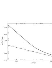
Figure 2: Left panel: The static Coulomb potential. Right panel: The three-gluon vertex at the symmetric point, full line with non-perturbative propagators, dashed line with perturbative propagators.

Let me stress that it is absolutely crucial to keep fully the Faddeev-Popov determinant $J[A]$ in both the Hamiltonian and the integration measure. The Faddeev-Popov determinant converts the flat integration measure $\int{\cal D}A$ into the Haar measure of the gauge group Reinhardt:1996fs . When the Faddeev-Popov determinant is neglected Szczepaniak:2001rg the gluon energy becomes infrared finite and the linear rise in the static color potential is lost. On the other hand, the obtained infrared behavior is quite robust with respect to changes of the variational wave functional. Extending the variational ansatz, eq. (2), to arbitrary $\alpha$ (where $\alpha=\frac{1}{2}$ and $\alpha=0$ correspond to the wave functional used in refs. Feuchter:2004mk and Szczepaniak:2001rg , respectively), it can be shown that up to two loops in the energy, the variational solution and in particular the ghost and gluon propagators are actually independent of $\alpha$, see ref. Reinhardt:2004mm . Other quantities like the three-gluon vertex are, however, more sensitive than the energy and do depend on $\alpha$.

The leading contribution to the three-gluon vertex is given by the triangle diagram with an internal ghost loop. In this order the three-gluon vertex has the same color structure as the bare one and can be expressed by a single form factor

$$\Gamma^{abc}_{ijk}\left(p_{1},p_{2},p_{3}\right)=f^{abc}\left(i(p_{1})_{j}\delta_{ik}F\left(p_{1},p_{2},p_{3}\right)+\mbox{permutations}\right)\hskip 2.84544pt.$$ (11)

The form factor $F$ is shown in fig. 2 for the symmetric point $p_{1}=p_{2}=p_{3}$. The infrared analysis performed in ref. Schleifenbaum:2006bq shows $F(p^{2})\sim(p^{2})^{\frac{d}{2}-2-\frac{3}{2}\beta}$. Inserting here $d=3$ and $\beta=0.85$ from ref. Feuchter:2004mk , one finds $F(p^{2})\sim(p^{2})^{-1.775}$, which is in perfect agreement with the numerical result shown in fig. 2, from which one extracts $F(p^{2})\sim(p^{2})^{-1.77}$. We have also investigated the ghost-gluon vertex and found that, like in Landau gauge, it becomes bare when one of the external ghost momenta vanishes, so that its dressing can be ignored, at least in the infrared.

We can define the RG-invariant running coupling constant,

$$\alpha(k)=\frac{16}{3}\frac{g^{2}_{R}}{4\pi}p^{5}G^{2}(p)D(p)\,,$$ (12)

from the ghost-gluon vertex Fischer:2005qe , where $G(p)$ and $D(p)$ are the ghost and gluon propagators, respectively. Due to the sum rule (9) for the infrared exponents this coupling has an infrared fixed point which for the DSE solutions with $\beta=1.0$ is given by $\alpha(0)=16\pi/(3N_{c})\approx 16.76/N_{c}$, see ref. Schleifenbaum:2006bq . This value obtained in the infrared analysis is in excellent agreement with the value of $\alpha(0)=16.94/N_{c}$, see Epple , which is obtained from the numerical solution of the DSE presented in fig. 1. Let us also stress that this result disagrees with the value for the infrared fixed point obtained in the Coulomb gauge limit of the interpolating gauges Fischer:2005qe .

3 The ’t Hooft loop

The class (2) of wave functionals yield (up to two loops in the energy) the same Dyson-Schwinger equations independent of $\alpha$. To test our wave functional and to get more detailed information on the structure of the Yang-Mills vacuum, observables more sensitive than the energy density should be calculated. Moreover, the confining Coulomb potential obtained above does not necessarily guarantee that our wave functional describes indeed a confining vacuum state. The reason is that the Coulomb potential is only an upper-bound to the true static quark potential Zwanziger . Thus a confining Coulomb potential is a necessary but not a sufficient condition for a confining vacuum.

In pure Yang-Mills theory the order parameter of confinement is the temporal Wilson loop, which obeys an area law in the confined phase and a perimeter law in the deconfined phase. Unfortunately, this quantity is difficult to calculate in the continuum theory due to the path ordering. Fortunately, there exists another (dis-)order parameter of Yang-Mills theory which is easier to calculate in the continuum theory. This is the spatial ’t Hooft loop which is dual to the temporal Wilson loop in the sense that it obeys a perimeter law in the confined phase and an area law in the deconfined phase 'tHooft:1977hy .

The operator $V(C)$ of ’t Hooft’s disorder parameter is defined for a spatial loop $C$ by the following relation 'tHooft:1977hy :

$$V(C_{1})W(C_{2})=Z^{L(C_{1},C_{2})}W(C_{2})V(C_{1})\quad,\quad W(C)=\frac{1}{N}tr\,P\exp(i\oint\limits_{c}A)$$ (13)

where $W(C)$ is the spatial Wilson loop, $Z$ is a (non-trivial) center element of the gauge group ($Z=-1$ for SU(2)) and $L(C_{1},C_{2})$ denotes the Gaussian linking number between the two spatial loops $C_{1}$ and $C_{2}$. Unfortunately ’t Hooft did not give an explicit realization of the operator $V(C)$ in the continuum theory, but defined the operator implicitly as having the effect of a singular (on the loop $C$) gauge transformation.

The physical meaning of the ’t Hooft loop defined by equation (13) is recognized by noticing that a time independent (spatial) center vortex ${\mathcal{A}}(C_{1})$ whose magnetic flux is localized on the closed loop $C_{1}$, produces the Wilson loop $W\big{[}\mathcal{A}(C_{1})\big{]}(C_{2})=Z^{L(C_{1},C_{2})}$. It follows that the ’t Hooft loop operator $V(C)$ can be interpreted as a center vortex creation operator. The operator $V(C)$ which generates a center vortex gauge field $\mathcal{A}(C)$ i.e., $V(C)\Psi(A)=\Psi\big{(}A+\mathcal{A}(C)\big{)}$, is given by

$$V(C=\partial\Sigma)=\exp\left(i\int d^{3}x\mathcal{A}^{a}_{i}(\Sigma,x)\Pi^{a}_{i}(x)\right).$$ (14)

In reference Reinhardt:2002mb it was proven that the operator (14) with the vortex field

$$\mathcal{A}^{a}_{i}(\Sigma,x)=\zeta^{a}\int_{\Sigma}d^{2}\tilde{\sigma_{i}}\delta^{3}(x-\bar{x}(\sigma))$$ (15)

with $\zeta=\zeta^{a}T_{a}$ being a co-weight vector defined by $\exp(i\zeta)=Z$ actually satisfies the defining relation (13). Since $\Pi^{a}_{i}(x)$ is the operator of the electric field, the ’t Hooft loop measures the electric flux (projected on the co-weight $\zeta=\zeta^{a}T_{a}$) through the closed loop $C$, while the (spatial) Wilson loop $W(C)$ measures the magnetic flux through $C$. The operator $V(C)$ is not manifestly gauge invariant, but produces a gauge invariant result, when acting on gauge invariant states $\Psi(A^{U})=\Psi(A)$.

The wave functional in Coulomb gauge satisfies Gauss’ law (which ensures gauge invariance) and has, hence, to be considered as the restriction of the gauge invariant wave functional to transverse gauge fields. Therefore by implementing the Coulomb gauge by the standard Faddeev-Popov method, we obtain for the ’t Hooft loop

$$\langle V(C)\rangle=\int\mathcal{D}A\,J(A)\,\Psi^{\ast}(A)\,\Psi(A+\mathcal{A}^{\perp}(C)\big{)}\hskip 2.84544pt,$$ (16)

where $\mathcal{A}^{\perp}(C=\partial\Sigma)$ is the transverse part of the center vortex field $\mathcal{A}(\Sigma)$ (15) given by Reinhardt:2001kf

$$\mathcal{A}^{\perp}(\partial\Sigma,x)=-\zeta\oint_{\partial\Sigma}d\tilde{\sigma}_{ik}\partial^{\bar{x}}_{k}\,\frac{1}{4\pi|x-\bar{x}|}\quad,\quad d\tilde{\sigma}_{ik}=\Sigma_{ik\ell}\,d\bar{x}_{\ell}$$ (17)

which manifestly depends only on the loop $C=\partial\Sigma$ but not on the enclosed surface $\Sigma$ as the field (15) does. It is straightforward to calculate from eq. (17) ’t Hooft’s disorder parameter inserting for $\Psi(A)$ the wave functional determined previously Feuchter:2004mk . After straightforward calculations, one finds

$$\langle V(C)\rangle=\exp(-S)\hskip 2.84544pt,\hskip 2.84544ptS(C)=\int^{\infty}_{0}dq\,K(q)\,h(C,q)\hskip 2.84544pt,$$ (18)

where

$$K(q)=\frac{1}{2}\omega(q)\,\big{(}1-\frac{\chi^{2}(q)}{\omega^{2}(q)}\big{)}$$ (19)

contains the whole information about Yang-Mills vacuum while the quantity $h(C,q)$ is exclusively determined by the geometry of the considered loop. To simplify the calculations of this quantity, we consider a planar circular loop with radius $R$. A detailed analysis shows that the $R$ dependence of $S(R)$ is determined by the infrared behavior of $K(q)$. Given that $\omega(q)$ and $\chi(q)$ are both infrared divergent and differ only by a finite constant, one finds

$$K(q\to 0)=\big{(}\omega(q)-\chi(q)\big{)}_{q\to 0}=c$$ (20)

where $c$ is a finite renormalization constant which can be chosen arbitrarily. Choosing $c=0$, which implies that the infrared wave functional reduces to the strong coupling limit $\Psi[A]=1$, one finds indeed a perimeter law ${S}(R)=\tilde{\kappa}R$, while for $c\neq 0$ one obtains ${S}R\sim R\,\ln(R/R_{0})$. Finally, if one ignores the curvature $(\chi=0)$ in eq. (19), one finds an area law ${S}(R)=\tilde{\varrho}R^{2}$. Thus again we find the curvature to be crucial for the confinement properties of the theory.

4 Summary and Conclusions

In my talk I have discussed recent results obtained in the Hamilton approach to Yang-Mills theory in Coulomb gauge. Using ghost dominance, an infrared analysis of the Schwinger-Dyson equations has revealed both quark and gluon confinement. The gluon energy is infrared diverging implying the absence of asymptotic gluon states from the physical spectrum, and the static Coulomb potential is linearly rising. These results are confirmed by a full numerical solution of the Schwinger-Dyson equations. While the ghost-gluon vertex remains basically unrenormalized and in particular becomes the bare one when the ghost momentum vanishes, the three-gluon vertex is strongly infrared divergent. As a first non-trivial test of the variationally determined vacuum wave functional, we have calculated ’t Hooft’s disorder parameter choosing the renormalization constants of the gap equation in such a way that the wave functional reproduces in the infrared the strong coupling limit. Then the ’t Hooft loop shows indeed a perimeter law, indicating a confining vacuum.

References

- (1) R. G. Leigh, D. Minic and A. Yelnikov, Phys. Rev. Lett. 96 (2006) 222001 [arXiv:hep-th/0512111].
- (2) C. Feuchter and H. Reinhardt, Phys. Rev. D 70, 105021 (2004) [arXiv:hep-th/0408236].
- (3) N. H. Christ and T. D. Lee, Phys. Rev. D 22, 939 (1980) [Phys. Scripta 23, 970 (1981)].
- (4) A. P. Szczepaniak and E. S. Swanson, Phys. Rev. D 65, 025012 (2002) [arXiv:hep-ph/0107078].
- (5) W. Schleifenbaum, M. Leder and H. Reinhardt, Phys. Rev. D 73, 125019 (2006) [arXiv:hep-th/0605115].
- (6) D. Zwanziger, Nucl. Phys. B 485 (1997) 185 [arXiv:hep-th/9603203].
- (7) D. Zwanziger, Phys. Rev. D 65 (2002) 094039 [arXiv:hep-th/0109224], C. Lerche and L. von Smekal, Phys. Rev. D 65 (2002) 125006 [arXiv:hep-ph/0202194].
- (8) J. C. Taylor, Nucl. Phys. B 33 (1971) 436, W. Schleifenbaum, A. Maas, J. Wambach and R. Alkofer, Phys. Rev. D 72 (2005) 014017 [arXiv:hep-ph/0411052].
- (9) C. S. Fischer and D. Zwanziger, Phys. Rev. D 72, 054005 (2005) [arXiv:hep-ph/0504244].
- (10) D. Epple, H. Reinhardt and W. Schleifenbaum, to be published.
- (11) H. Reinhardt, Mod. Phys. Lett. A 11, 2451 (1996) [arXiv:hep-th/9602047].
- (12) H. Reinhardt and C. Feuchter, Phys. Rev. D 71, 105002 (2005) [arXiv:hep-th/0408237].
- (13) D. Zwanziger, Phys. Rev. Lett. 90 (2003) 102001 [arXiv:hep-lat/0209105], J. Greensite, S. Olejnik and D. Zwanziger, Phys. Rev. D 69 (2004) 074506 [arXiv:hep-lat/0401003].
- (14) G. ’t Hooft, Nucl. Phys. B 138, 1 (1978).
- (15) H. Reinhardt, Phys. Lett. B 557, 317 (2003) [arXiv:hep-th/0212264].
- (16) H. Reinhardt, Nucl. Phys. B 628, 133 (2002) [arXiv:hep-th/0112215], M. Engelhardt and H. Reinhardt, Nucl. Phys. B 567 (2000) 249 [arXiv:hep-th/9907139].