Uplifting and Inflation with D3 Branes

Abstract:

Back-reaction effects can modify the dynamics of mobile D3 branes moving within type IIB vacua, in a way which has recently become calculable. We identify some of the ways these effects can alter inflationary scenarios, with the following three results: ($1$) By examining how the forces on the brane due to moduli-stabilizing interactions modify the angular motion of D3 branes moving in Klebanov-Strassler type throats, we show how previous slow-roll analyses can remain unchanged for some brane trajectories, while being modified for other trajectories. These forces cause the D3 brane to sink to the bottom of the throat except in a narrow region close to the D7 brane, and do not ameliorate the $\eta$-problem of slow roll inflation in these throats; ($2$) We argue that a recently-proposed back-reaction on the dilaton field can be used to provide an alternative way of uplifting these compactifications to Minkowski or De Sitter vacua, without the need for a supersymmetry-breaking anti-D3 brane; and ($3$) by including also the $D$-term forces which arise when supersymmetry-breaking fluxes are included on D7 branes we identify the 4D supergravity interactions which capture the dynamics of D3 motion in D3/D7 inflationary scenarios. The form of these potentials sheds some light on recent discussions of how symmetries constrain $D$ term interactions in the low-energy theory.

1 Introduction

Of late there has been considerable interest in understanding the dynamics of time-dependent string configurations largely motivated by their possible applications to cosmology, particularly to the search for inflation. The resulting dynamics has begun to produce a number of interesting scenarios for inflationary constructions, such as the brane-antibrane mechanism [1]-[6], D3/D7 models [7, 8], modular inflation [9] and other scenarios [10]-[12].

The study of the motion of branes within type IIB geometries with fluxes has been of particular interest, given the progress towards modulus stabilization which these geometries provide [13]-[16]. The goal of these studies is to improve the control over the approximations being made, in an effort to more reliably tie the time-dependent behaviour to the properties of real string vacua. What makes these studies difficult is the necessity of exploring nonsupersymmetric configurations when exploring time-dependent solutions, with the loss of control over the corrections to the leading features that this supersymmetry breaking entails.

The greater calculational control offered by supersymmetry makes it advantageous to keep any supersymmetry breaking parameterically small, putting a premium on constructions which can be regarded as only small deviations from the supersymmetric limit. In particular, this makes it preferable not to break supersymmetry with antibranes, since these necessarily require that supersymmetry be nonlinearly realized. This motivates identifying dynamical situations where supersymmetry breaks spontaneously, but in a way which allows a description of the low-energy dynamics purely in terms of a 4D supergravity. The motion of a mobile, or itinerant, D3 brane moving in the presence of background fluxes and the fields generated by various D7 and O7 sources provides an attractive class of systems of this type.

In this paper we use recent calculations [18, 20] of the back-reaction of such an itinerant D3 brane on the low-energy gauge coupling functions to identify some of the forces acting on the mobile D3. The first of these forces is described in the low-energy theory by an $F$-term potential [18], which arises because the low-energy superpotential acquires a dependence on the low-energy gauge coupling function due to nonperturbative effects. These can arise either through Euclidean D3-branes wrapping a 4-cycle of the Calabi-Yau (CY) [21], or by gaugino condensation [22] of an unbroken gauge group living on a stack of D7 branes which also wrap a 4-cycle in the CY. The potential induced in this way was identified some time ago [3] as the source of an $\eta$ problem for inflationary models involving mobile D3 branes moving in the throat; ignorance of its detailed form left open the possibility [3] – [6] that inflation could nonetheless be achieved by adjusting inflaton-dependent corrections to the superpotential. But this begged the question of whether string theory really provides the desired kind of superpotential corrections.

Progress toward computing this superpotential more explicitly was recently made by ref. [18], who noted that the form of the superpotential corrections can be explicitly calculated for branes moving within a Klebanov-Strassler (KS) throat [23, 24], if the wrapped 4-cycle is itself within the throat. In section §2 we use this calculation to compute the motion of a mobile D3 brane, and find that the resulting superpotential vanishes when minimized along the angular directions which parameterize the 5D $T^{1,1}$ submanifold of the throat. We conclude that the superpotential by itself therefore does not counteract the $\eta$ problem for motion along these directions. Furthermore, the forces which push the D3 brane in the angular directions are too steep to provide new slow-roll mechanisms themselves.

An additional force on the D3 brane also arises at the same order as the superpotential correction, due to the back-reaction of the D7 brane on the background dilaton profile [25]. We find in §3 that this force competes with that due to the superpotential in such a way as to change the stable point of the D3 motion in the angular directions in the throat. However including these corrections does not allow one to fine-tune away the $\eta$-problem of slow roll inflation, since they provide a force on the D3 brane which is in the same direction as the force which gives rise to the $\eta$ problem. On the other hand, we show that because the dilaton correction increases the potential energy of the D3, it can be used to uplift the vacuum to de Sitter or Minkowski space, even in the absence of an antibrane. This new possibility may allow better control over the corrections to this picture inasmuch as it does not rely on the introduction of badly-broken supersymmetry via antibranes.

Finally, in section §4 we use the modified gauge kinetic functions of ref. [18] to compute the force on a mobile D3 brane which arises when supersymmetry-breaking fluxes are introduced on the D7 branes, due to the partial failure of the BPS cancellations amongst the interbrane forces. This type of force has been argued to be described by a $D$-term potential [26]-[28], whose form has also been recently identified by other workers [29]. We identify the $F$ and $D$ terms which describe the motion of a D3 in the special case that the internal dimensions have the form of a product of a 4-cycle with two toroidal (or orbifold) dimensions (such as for $K3\times T^{2}/\mathbb{Z}_{2}$). Besides expecting these results to be pertinent for constructing new inflationary scenarios, we find they also provide useful illustrations of how the low-energy theory implements some of the symmetries which arise when discussing $D$-term potentials.

1.1 D3’s and D7’s in type IIB vacua

In type IIB compactifications the perturbations to the strength of gauge couplings on nearby D7 branes due to the presence of itinerant D3 branes within the bulk have recently been calculated in two independent ways. They were first obtained as loop-generated threshold effects within an open-string picture [20], with the result in some instances reconfirmed by performing a back-reaction calculation within the closed-string picture [18].

The background spacetimes which arise within warped type IIB compactifications preserving $N=1$ supersymmetry in four dimensions [13, 14] have the general form

$${\rm d}s^{2}=h^{-1/2}(y)\,g_{\mu\nu}(x)\,{\rm d}x^{\mu}{\rm d}x^{\nu}+h^{1/2}(y)\,\tilde{g}_{mn}(y)\,{\rm d}y^{m}{\rm d}y^{n}\,,$$ (1)

where $h(y)$ denotes the warp factor. Given this metric, the gauge term for a massless gauge field situated on a stack of coincident space-filling D7 brane becomes

$$S_{g}=-\frac{1}{4}\int_{\Sigma}d^{4}x\sqrt{-g_{4}}\;g^{\mu\nu}g^{\lambda\rho}{\cal G}_{ab}F^{a}_{\mu\lambda}F^{b}_{\nu\rho}\,,$$ (2)

where the matrix ${\cal G}_{ab}$ governs the effective gauge coupling strength, and is given semiclassically by the following warped volume

$${\cal G}_{ab}={\cal T}_{7}V_{\Sigma}^{w}\delta_{ab}\equiv{\cal T}_{7}\,\delta_{ab}\int_{\Sigma}d^{4}y\sqrt{\tilde{g}_{4}}\;h\,,$$ (3)

where $a$, $b$ label gauge group generators, $\Sigma$ denotes the 4-cycle wrapped by the 7-brane in the internal 6 dimensions and ${\cal T}_{7}\propto\alpha^{\prime 2}T_{7}$ is proportional to the 7-brane tension.

For compactifications which preserve $N=1$ supersymmetry in 4D, supersymmetry dictates that ${\cal G}_{ab}$ must be the real part of a holomorphic quantity when it is viewed as a function of the moduli which appear as fields within the low-energy 4D theory. For instance, if we follow in this way the dependence on the volume modulus for the internal dimensions, $\tilde{g}_{mn}=e^{2u}\,g_{mn}$, we see that ${\cal G}_{ab}\propto e^{4u}\,\delta_{ab}$. In the absence of the itinerant D3 branes of interest below, this is indeed the real part of a holomorphic function because it is related to the holomorphic volume modulus, $\rho$, by

$$e^{4u}=\rho+\overline{\rho}\,.$$ (4)

D3 perturbations to D7 gauge couplings

When identifying forces acting on the D3’s our interest is in how the above expressions respond to the presence of a perturbing mobile D3 brane situated at a point $y^{m}=z^{m}$ in the bulk, since we wish to follow how the low-energy 4D theory depends on the position modulus, $z^{m}$. From the microscopic point of view, this involves determining how the the quantity ${\cal G}_{ab}$ responds to the back-reaction of the 10D geometry to the 3-brane’s position. ${\cal G}_{ab}$ depends on this back-reaction because the gauge couplings depend on the volume of the cycle which the D7 wraps, and this becomes corrected by the change in the bulk geometry due to the presence of the itinerant D3 brane.

As was recently emphasized [18], the holomorphy of this back-reaction enters in two ways: through perturbations to the volume, $e^{4u}$, and to perturbations to $h$. Although both of these perturbations introduce nonholomorphic contributions to ${\cal G}_{ab}$, these contributions cancel to leave a holomorphic brane-dependent contribution to the gauge kinetic function: ${\cal G}_{ab}\propto\delta_{ab}\,\hbox{Re}\,f$ with $f=\rho+F(z)$, in agreement with the earlier arguments of [20]. The quantity $F(z)$ here represents a suitable cycle average of the holomorphic part of the appropriate Greens function which governs the perturbations $\delta e^{4u}$ and $\delta h$.

1.2 Forces on itinerant D3 branes

Although all static forces cancel (by definition) between an itinerant D3 brane and the other branes in a lowest-order supersymmetric construction, typically this no longer remains true once all corrections are taken into account. For sufficiently slow motion the dynamics generated by these forces can be described within a low-energy effective 4D theory, whose comparative simplicity is often a prerequisite for being able to fully analyze the motion. Furthermore, provided that the size of the supersymmetry breaking associated with the forces is kept small enough the result must be a particular kind of $N=1$ 4D supergravity. An approximately supersymmetric 4D limit of this type is particularly powerful because of the control it provides over the approximations underlying the compactification which leads to the effective 4D Lagrangian.

The key to understanding the 4D supergravity formulation lies with the gauge kinetic function given in the previous section, which have the generic form ${\cal G}^{s}_{ab}={\cal T}_{7}V_{\Sigma}^{i}\,\delta_{ab}\left(f_{s}+\overline{f_{s}}\right)$ with

$$f_{s}(\rho,z)=\rho+F_{s}(z)\,.$$ (5)

Here the subscript ‘$s$’ labels the relevant D7 brane on which lives the corresponding massless gauge field. This dependence of gauge couplings on D3 brane positions gives rise to two kinds of forces of this type which are of particular interest.

$F$-terms and volume-stabilization forces

There are forces on the D3 brane arising from any dynamics (like gaugino condensation or D3 instantons) which stabilize the various moduli of the bulk geometry. These mediate a force on the itinerant D3 because the moduli typically adjust in the supersymmetric case as the D3 moves, as required in order to keep the net force on the D3 zero. Any energetic cost for making this adjustment indirectly induces a potential which depends on the D3 position. This leads to the force which so complicated the inflationary analysis within warped throats [3, 6]

The interaction potential generated in 4D by modulus stabilization is incorporated by using the kinetic function, eq. (5), within the standard superpotentials which are used in the literature to describe the gaugino condensation (or D3 instanton) which stabilizes the relevant moduli [15, 18, 22]:

$$W=W_{0}+\sum_{s}A_{s}\exp\Bigl{[}-a_{s}f_{s}(\rho,z)\Bigr{]}\,.$$ (6)

Here the constant $W_{0}$ expresses the effects of any supersymmetry-breaking amongst the higher-dimensional fluxes which stabilize some of the moduli, while the exponential term contains the influence of gaugino condensation (or the like) on various D7 branes, and involves the dependence on the D3 position due to the back-reaction of the D3 onto the relevant gauge coupling strengths. The quantities $A_{s}$ and $a_{s}$ are $z$-independent constants which are calculable given the details of the underlying physics.

$D$-terms and direct interbrane forces

A supersymmetry-breaking flux localized on any of the branes also introduces a direct interbrane force, independent of the stabilization of bulk moduli. It does so because the breaking of supersymmetry ruins the BPS cancellations among the long-range bulk forces corresponding to the exchange of massless closed-string states. This typically leads to an interbrane potential which varies near a source brane like $r^{2-d}$, where $d$ counts the number of transverse dimensions. (For $d=2$ the potential becomes logarithmic.) It gives rise to the attractive force which is used in most brane-antibrane [2] and D3/D7 [7, 8] inflationary analyses.

A similar argument can be used to incorporate the effects of imperfect cancellation of bulk forces due to supersymmetry-breaking fluxes localized on various branes. To this end, imagine turning on a background gauge field, ${\cal F}_{mn}$, on a 7-brane, which at the classical level contributes a 4D Einstein-frame action of the form

$$S_{f}=-{\cal T}_{7}\int d^{\,4}x\sqrt{g_{4}}\;{\cal H}\,,$$ (7)

where

$${\cal H}=\int_{\Sigma}d^{4}y\sqrt{g_{4}}\;e^{-12u}h^{-1}g^{mn}g^{pq}{\cal F}_{mp}{\cal F}_{nq}$$ (8)

If the fluxes involved break supersymmetry by a sufficiently small amount, then it has been argued [26]-[28] that such a flux term contributes a $D$-term potential to the low-energy effective 4D supergravity, of the form

$$V_{D}=\frac{1}{2}\,{\cal G}^{ab}D_{a}D_{b}\,,$$ (9)

where ${\cal G}^{ab}$ is the inverse of the matrix, ${\cal G}_{ab}$, of holomorphic gauge-kinetic functions, and the sum is over the generators of the group gauged by the massless spin-1 particles. Here

$$D_{a}=\xi_{a}+{\cal D}_{a}$$ (10)

where ${\cal D}_{a}=\partial_{i}K(\varphi,\overline{\varphi})[t_{a}\varphi]^{i}$ represents the $D$-term contribution of any charged scalar matter fields in the low-energy theory, and $\xi_{a}$ represents a field-dependent Fayet-Iliopoulos (FI) term [30], which can only arise for $U(1)$ factors of the gauge group.

2 D3 dynamics in warped throats

We next turn to a more detailed exploration of the implications of these forces for the specific case of D3 motion in the strongly warped region of the internal geometry. The internal geometry will turn out to be more complicated than the simple deformed conifold case studied earlier. In fact the susy breaking for our case will be intimately tied up with some specific features of the internal geometry. In the following section we will elaborate this story.

2.1 Internal geometry and supersymmetry breaking

We therefore begin by analysing the precise background metric for our case. In terms of eq. (1) we aim to determine $\tilde{g}_{mn}$ that would include the backreactions from the D7 branes, D3 branes and fluxes, as well as some controlled nonperturbative effects such as gaugino condensates on the D7 branes. The warp factor $h$ appearing in (1) already takes into account some of these effects, but there are in addition some subtle changes to the standard deformed conifold background that are responsible for breaking supersymmetry in our case. In fact we soon argue that even after we switch off the nonperturbative SUSY-breaking effects, the resulting background still breaks supersymmetry because the backreactions from the D7 and the D3 branes do not allow primitive three-form fluxes in this geometry.

The three-form fluxes are the $H_{3}=H_{NS}$ and $F_{3}=H_{RR}$ which would satisfy the equations of motion if $G_{3}\equiv F_{3}+\tau H_{3}$ is imaginary self-dual (ISD) where $\tau$ is the axio-dilaton. We can view the RR component of $G_{3}$ as coming from a dual theory with wrapped D5 branes.

The metric now can be computed using various arguments. In the absence of itinerant D3 branes, the background with D7 branes and fluxes could be supersymmetric. Ouyang [25] has computed the metric of D7 branes with fluxes on a Klebanov-Tseytlin type geometry [31] by regarding the D7 branes as probes in the background. The final metric therein has an overall warp factor $h$ (much like (1)) with $\tilde{g}_{mn}$ being given by the Klebanov-Tseytlin metric [31]. However there are two shortcomings: one, the geometry should be given by a full F-theory picture, and two, the metric $\tilde{g}_{mn}$ should be the Klebanov-Strassler type metric [24]. These shortcomings are not very severe as long as we are away from the tip of the Klebanov-Strassler throat, and consider the geometry only in the neighborhood of one D7 brane. On the other hand, once we try to incorporate all the branes the global geometry becomes very complicated and we can only infer the local picture in certain cases [32].

Here we try to address the noncompact limit of our global geometry when additional D3 branes are also incorporated into the picture. From the considerations of [32] and [33] (see also [40]) the metric of the internal space looks like:

$${\rm d}s^{2}=F_{1}~{}(e_{1}^{2}+e_{2}^{2})+F_{2}\sum_{i=1}^{2}~{}(\epsilon_{i}^{2}-2be_{i}\epsilon_{i})+v^{-1}(\epsilon_{3}^{2}+{\rm d}r^{2})\,,$$ (11)

where $F_{i}$ are some functions of the radial coordinate $r$, ($v,b$) are parameters, and ($e_{i},\epsilon_{i}$) are defined as

$$e_{1} = {\rm d}\theta_{1},~{}~{}~{}~{}~{}~{}e_{2}=-{\rm sin}~{}\theta_{1}{\rm d}\phi_{1}\,,$$

$$\epsilon_{1} = {\rm sin}~{}\psi~{}{\rm sin}~{}\theta_{2}{\rm d}\phi_{2}+{\rm cos}~{}\psi~{}{\rm d}\theta_{2}\,,$$

$$\epsilon_{2} = {\rm cos}~{}\psi~{}{\rm sin}~{}\theta_{2}{\rm d}\phi_{2}+{\rm sin}~{}\psi~{}{\rm d}\theta_{2}\,,$$

$$\epsilon_{3} = {\rm d}\psi+{\rm cos}~{}\theta_{1}{\rm d}\phi_{1}+{\rm cos}~{}\theta_{2}{\rm d}\phi_{2}\,.$$ (12)

We see that the background is neither Klebanov-Tseytlin nor Klebanov-Strassler because there are two two-spheres – given by $\sum_{i}e_{i}^{2}$ and $\sum_{i}\epsilon_{i}^{2}$ – that have unequal radii. In fact the radii are given by $F_{1}(r)$ and $F_{2}(r)$ respectively. Once we remove the D7 branes, the $F_{i}$ take the following form [34]

$$F_{1}(r)=e^{g}+b^{2}\,e^{-g},~{}~{}~{}~{}~{}~{}~{}~{}F_{2}(r)=e^{-g}\,,$$ (13)

where $g=g(r)$ whose functional form can be extracted from [34], and $b$ measures the size of the three-cycle at the tip of the throat. On the other hand, if we remove the D3 branes and put in a single D7 brane, then the background will be close to the one predicted by Ouyang [25] with $F_{1}\approx F_{2}$ but with a naked singularity at the tip. If we replace the naked singularity with a nontrivial three-cycle then the local geometry is given in [32] with $F_{1}\neq F_{2}$. Thus incorporating all the branes and fluxes, the geometry around the neighborhood of the D3 and the D7 branes will clearly be (11) with $F_{1}\neq F_{2}$.

To study the issue of supersymmetry, let us take the limit $b\to 0$. In this limit our background looks like a warped resolved conifold with $G_{3}$ fluxes and branes. Supersymmetry will be preserved if we can argue that $G_{3}$ is a pure (2,1) form with vanishing (1,2), (3,0) and (0,3) components. Recall that this condition is stronger than the ISD condition imposed on the $G_{3}$ fluxes.

The background supergravity equations of motion connect these forms to radii of various cycles in the internal manifold (11). For example, a direct computation of background fluxes along the lines of [35] reveals that $G_{3}$ has both (2,1) as well as (1,2) components given in the following way:

$$G_{3}~{}=~{}(F_{1}^{-1}+F_{2}^{-1})\Lambda^{2,1}~{}\oplus~{}(F_{1}^{-1}-F_{2}^{-1})\Lambda^{1,2}\,,$$ (14)

and would become supersymmetric when $F_{1}=F_{2}$ globally. Here we have denoted the (2,1) and (1,2) forms by $\Lambda^{2,1}$ and $\Lambda^{1,2}$ respectively. Locally imposing this cancellation implies that the regime of interest has $G_{3}\propto\Lambda^{2,1}$ with vanishing (1,2) piece. However it would be wrong to conclude that supersymmetry is restored! Only under strict global cancellation of the (1,2) part could we infer unbroken supersymmetry. From the analysis presented here (along with the earlier references) it seems difficult to have $F_{1}=F_{2}$ everywhere in the internal space.

Consider now the case when $F_{1}\neq F_{2}$ but $H_{3}=0$ and $F_{3}\neq 0$. This could in principle happen when we are in the far-IR region of the geometry. Now of course the concept of (2,1) and (1,2) forms makes no sense as $G_{3}$ is real. Is SUSY restored for our case? The answer is no because in the presence of $F_{3}$ and $F_{1}\neq F_{2}$, a D7 brane breaks all supersymmetry. Therefore we see that SUSY could in principle be broken by two effects in the background (11): non-primitive $G_{3}$ fluxes and D7 branes. Both these effects are somehow connected to having $F_{1}\neq F_{2}$.

2.2 The superpotential correction

We now return to our starting point, the warped solution, eq. (1), where ${\rm d}s_{6}^{2}$ given by the metric (11) and $h(r)$ is the warp factor. To simplify the ensuing analysis, let us first consider the following limits of the variable defined in (11):

$$b~{}\to~{}0,~{}~{}~{}~{}v~{}=~{}1,~{}~{}~{}~{}F_{1}(r)~{}\approx~{}F_{2}(r)~{}=~{}{r^{2}\over 6},~{}~{}~{}~{}~{}\epsilon_{3}~{}\to~{}{r\epsilon_{3}\over 3}\,.$$ (15)

which gives the conifold limit of the metric. We employ the standard idea that this manifold can be defined by the complex surface

$$w_{1}\,w_{2}-w_{3}\,w_{4}=0\,,$$ (16)

in four complex dimensions. The complex coordinates $w_{i}$ are related to real coordinates $(r,\theta_{1},\theta_{2},\phi_{1},\phi_{2},\psi)$ via

$$w_{1} = r^{3/2}\,e^{\frac{i}{2}(\psi-\phi_{1}-\phi_{2})}\sin\frac{\theta_{1}}{2}\,\sin\frac{\theta_{2}}{2}\,,$$

$$w_{2} = r^{3/2}\,e^{\frac{i}{2}(\psi+\phi_{1}+\phi_{2})}\cos\frac{\theta_{1}}{2}\,\cos\frac{\theta_{2}}{2}\,,$$

$$w_{3} = r^{3/2}\,e^{\frac{i}{2}(\psi+\phi_{1}-\phi_{2})}\cos\frac{\theta_{1}}{2}\,\sin\frac{\theta_{2}}{2}\,,$$

$$w_{4} = r^{3/2}\,e^{\frac{i}{2}(\psi-\phi_{1}+\phi_{2})}\sin\frac{\theta_{1}}{2}\,\cos\frac{\theta_{2}}{2}\,,$$ (17)

In terms of these real coordinates, the metric of the conifold can be written explicitly,

$${\rm d}s_{6}^{2}={\rm d}r^{2}+r^{2}\left[\frac{1}{9}\left({\rm d}\psi+\sum_{i=1}^{2}\cos\theta_{i}\,{\rm d}\phi_{i}\right)^{2}+\frac{1}{6}\sum_{i=1}^{2}\left({\rm d}\theta_{i}^{2}+\sin^{2}\theta_{i}\,{\rm d}\phi_{i}^{2}\right)\right]\,.$$ (18)

As emphasised before, the limit (15) provides a good approximation only for intermediate ranges within a throat for two reasons. First, in this regime $G_{3}$ is a pure (2,1) form and the complications due to the other components do not show up; and secondly our results do not depend on these complications associated with $b\neq 0$, since all the action will be taking place away from the bottom of the throat.

The Kähler potential for the moduli of such a configuration is known to be [36]

$$\kappa_{4}^{2}K=-3\log\left[2\sigma-c\,k(w_{i},\bar{w}_{i})\right]\,,$$ (19)

where $c=\frac{1}{3}\kappa_{4}^{2}T_{3}$ and $2\sigma=\rho+\bar{\rho}$. The quantity $k$ denotes the Kähler potential of the Calabi-Yau space itself — in our case, the conifold — which is given by [38, 39]

$$k(w_{i},\bar{w}_{i})=r^{2}=\left(\sum_{i=1}^{4}|w_{i}|^{2}\right)^{2/3}\,.$$ (20)

This form can be inferred in various ways, for example by comparing the D3-brane kinetic term in the present SUGRA description with the expression that results from evaluating the DBI action in the compactified background.

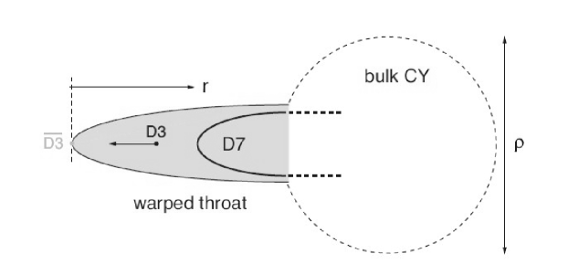
Figure 1: A cartoon (taken from ref. [18]) of the configuration of D3 and D7 branes used in the superpotential calculation.

To follow the explicit D3 dynamics we use the KKLT superpotential, supplemented by the $w_{i}$-dependent corrections discussed above, which are computed in ref. [18] for the case where gaugino condensation occurs on a stack of D7’s which wrap a cycle extending into the throat, specified by the supersymmetric embedding

$$\prod_{i=1}^{4}w_{i}^{p_{i}}=\mu^{P}\,,$$ (21)

as in Fig. (1). The resulting superpotential can be taken from (6) and rewritten as

$$W=W_{0}+A(w_{i})e^{-a\rho}$$ (22)

where

$$A(w_{i})=A_{0}\left(1-{\prod_{i=1}^{4}w_{i}^{p_{i}}\over\mu^{P}}\right)^{1/N_{D7}}$$ (23)

with $P=\sum_{i}p_{i}$ and $N_{D7}$ the number of D7 branes. In the special case of $N_{D7}=1$ there is no gaugino condensation, but the Euclidean D3-brane mechanism [21] could instead apply. This superpotential can be thought of as a function of the distance between the D3 brane and the 4-cycle. In principle, there is a connection between the value of $a$ and the volume of the 4-cycle [18], $a=2T_{3}V_{\Sigma_{4}}/N_{D7}$, but for the pure conifold this volume diverges, and would only be cut off by the gluing of the throat to a bulk Calabi-Yau. Since this procedure is model-dependent, we are free to consider $a$ as a free parameter.

2.3 D3 dynamics

To compute the resulting D3 dynamics we first need to compute the F-term potential, given by the usual supergravity formula

$$V_{F}=e^{\kappa_{4}^{2}K}\left(K^{\bar{b}a}D_{a}W\overline{D_{b}W}-3\kappa_{4}^{2}|W|^{2}\right)$$ (24)

where the indices $a,b$ run over the complex fields $\rho,w_{i}$. It is possible to show that the inverse Kähler metric, $K^{a\bar{b}}$, is simple when expressed in block form, where the $\rho$ and $w_{i}$ fields are written in separate blocks. Defining the volume modulus as $R=\rho+\bar{\rho}-ck(w_{i},\bar{w}_{i})$, we find that $K^{a\bar{b}}$ has the form

$$K^{\bar{b}a}={R\over 3}\left(\begin{array}[]{c|c}R+ck_{,\bar{\imath}}k^{\bar{\imath}j}k_{,j}&k_{,\bar{\imath}}k^{\bar{\imath}a}\cr\hline\cr k^{\bar{b}i}k_{,i}&\frac{1}{c}k^{\bar{b}a}\cr\end{array}\right)$$ (25)

where $k^{\bar{\imath}j}$ is the inverse of $k_{i\bar{\jmath}}=\partial_{i}\partial_{\overline{\jmath}}k$. Furthermore, using the Kähler potential (20) we find that

$$k_{,\bar{\imath}}k^{\bar{\imath}a}=\frac{3}{2}w^{a};\qquad k^{\bar{b}i}k_{,i}=\frac{3}{2}\bar{w}^{b};\qquad k_{,\bar{\imath}}k^{\bar{\imath}j}k_{,j}=r^{2}\,,$$ (26)

implying that the combination $R+c\,k_{,\bar{\imath}}\,k^{\bar{\imath}j}k_{,j}$ appearing in (25) is simply $\rho+\bar{\rho}$.

Using these simplifications, the F-term potential takes the form

$$V_{F} = {\kappa_{4}^{2}\over 3R^{2}}\left[\phantom{\frac{1}{3}}\!\!\!\!(\rho+\bar{\rho})|W_{,\rho}|^{2}\right.-3(\overline{W}W_{,\rho}+{\rm c.c.})$$

$$\qquad\qquad\qquad+\left.\frac{3}{2}\left(\overline{W}_{,\bar{\rho}}w^{j}W_{,j}+{\rm c.c.}\right)+\frac{1}{c}k^{\bar{i}j}\overline{W}_{,\bar{i}}W_{,j}\right]{}$$

$$= {\kappa_{4}^{2}\over 3R^{2}}\Biggl{[}\left[(\rho+\bar{\rho})a^{2}+6a\right]|A|^{2}e^{-2a(\rho+\bar{\rho})}+3aW_{0}(Ae^{-a\rho}+\bar{A}e^{-a\bar{\rho}})$$

$$\qquad\qquad\qquad-\frac{3}{2}ae^{-a(\rho+\bar{\rho})}\left(\bar{A}w^{j}A_{,j}+{\rm c.c.}\right)+\frac{1}{c}k^{\bar{\imath}j}\overline{A}_{,\bar{\imath}}A_{,j}e^{-a(\rho+\bar{\rho})}\Biggr{]}\,,{}$$

which vanishes for a purely constant superpotential ($a=A_{i}=0$). The first line of (2.3) can be recognized as the KKLT potential before doing any uplifting. The second line in (2.3) contains the new contributions due to the $w_{i}$-dependent superpotential corrections. The KKLT potential would give an AdS minimum at $\sigma_{0}$ where $DW=0$ and

$$W_{0}=-A_{0}e^{-a\sigma_{0}}\left(1+\frac{2}{3}a\sigma_{0}\right),\quad\quad\quad V_{AdS}=-\frac{a^{2}A_{0}^{2}e^{-2a\sigma_{0}}}{6\sigma_{0}}\,.$$ (29)

The Ouyang embedding

We now focus on the simplest embedding, discussed by Ouyang [25], in which $p_{1}=1$ and $p_{i}=0$ for $i>1$. For simplicity we also take $N_{D7}=1$. We show that the superpotential corrections to $V_{F}$, denoted by $\delta V_{F}$, by themselves do not uplift, because they vanish when the polar angles of the $T^{1,1}$ space take their energetically preferred values, $\theta_{i}=0$. At small $\theta_{i}$, the $F$-term contribution takes the form

$$\delta V_{F}=M_{11}(\theta_{1}^{2}+\theta_{2}^{2})+M_{12}\cos\left(\textstyle\frac{1}{2}\tilde{\psi}\right)\theta_{1}\theta_{2}+\dots$$ (30)

where $\tilde{\psi}=\psi-\phi_{1}-\phi_{2}$. The determinant of the $\theta_{i}$ mass matrix is

$$\det M_{\theta\theta}=M_{11}^{2}-\textstyle\frac{1}{4}\cos^{2}\left(\textstyle\frac{1}{2}\tilde{\psi}\right)M_{12}^{2}\propto 1-a^{2}c^{2}\mu^{2}r$$ (31)

when evaluated at the supersymmetric KKLT minimum, eq. (29), and when we take $\cos(\textstyle\frac{1}{2}\tilde{\psi})=\pm 1$, which minimizes the potential for $\tilde{\psi}$.

The following argument shows that for reasonable values of $g_{s}$, $a^{2}c^{2}\mu^{2}r_{0}\ll 1$ (when $r$ is evaluated at the bottom of the throat), and hence $\theta_{i}=0$ indeed minimizes the F-term correction to the potential at a value where it vanishes. Suppose $R_{CY}$ is the Calabi-Yau radius, and $r_{0}=\xi_{0}L\sim\xi_{0}g_{s}^{1/4}/M_{s}$ in terms of the AdS curvature scale $L$ and the warp factor at the bottom of the throat, $\xi_{0}=h_{0}^{-1/4}$. Using $c\sim T_{3}/M_{p}^{2}\sim 1/(g_{s}R_{CY}^{6}M_{s}^{4})$, $a=2\pi/N$ for gaugino condensation of an $SU(N)$ gauge theory, and $\mu^{2}<R_{CY}^{3}$, we obtain

$$a^{2}c^{2}\mu^{2}r_{0}<\left(\frac{2\,\pi}{N}\right)^{2}{\xi_{0}\over g_{s}^{7/4}(R_{CY}\,M_{s})^{9}}$$ (32)

We need $R_{CY}M_{s}\gg 1$ for the validity of the low-energy effective theory, and since strong warping implies $\xi_{0}\ll 1$, the right-hand-side of (32) is generically $\ll 1$, unless the string coupling is taken to be much smaller than its normally assumed range of values. This shows that the curvature of the potential in the $\theta_{i}$ directions is positive at $\theta_{i}=0$, and implies that $\delta V_{F}$ has a local minimum at the poles of the $S^{3}$ within the $T^{1,1}$, along which $\delta V_{F}$ vanishes, for any values of the other coordinates within the conifold. Thus, the D3 brane likes to move to these poles along which the D3-dependence of the superpotential has no effect on the energy of the itinerant D3 brane.

We can repeat the previous argument for larger values of $r$ to see whether the situation can change higher in the throat. But even assuming that $r\sim\mu^{2/3}\sim R_{CY}$, the bound (32) is only softened to

$$a^{2}c^{2}\mu^{2}r<\left(\frac{2\,\pi}{N}\right)^{2}{1\over g_{s}^{2}(R_{CY}\,M_{s})^{8}}$$ (33)

Even without the warp factor on the right hand side, it would seem that having a large enough value of $R_{CY}\,M_{s}$ to justify the effective field theory approach makes it impossible to violate (33) without taking $g_{s}\ll(MsR_{CY})^{-4}$ — much smaller than the ${\cal O}(0.1)$ values usually entertained.

3 Dilaton corrections and uplifting

Interestingly there is a competing effect which could cause the brane to stabilize at nonvanishing polar angles, giving a positive uplifting energy to the brane. To study this we need to carefully analyse the backreactions of the D7 brane on the geometry. These backreactions will lead to possible running of the dilaton that will help us to study susy breaking effects more precisely.

3.1 D7 brane dynamics, running dilaton and D3 potential

The internal metric (11) alongwith the warp factor $h$ captures the effect of the D7 brane on the background volume $e^{4u}$, but the D7 brane also distorts the axion-dilaton background. This distortion is straightforward to work out using Ouyang’s embedding [25]. Denoting the axion-dilaton by $\tau$ we see that both $\tau$ and the axion $\tilde{\phi}$ can be denoted in the following way:

$$\tau~{}=~{}{i\over g_{s}}~{}+{N_{D7}\over 2\pi i}~{}{\rm log}~{}w_{1},~{}~{}~{}~{}~{}~{}\tilde{\phi}~{}=~{}{N_{D7}\over 4\pi}~{}(\psi-\phi_{1}-\phi_{2})$$ (34)

where $w_{1}$ is defined in (2.2) and $N_{D7}$ is the number of D7 branes. From (34) it is easy to see that the dilaton for our case is given by

$$e^{-\Phi}={1\over g_{s}}-{N_{D7}\over 2\pi}\log\left({r^{3/2}\over\mu}\sin{\theta_{1}\over 2}\,\sin{\theta_{1}\over 2}\right)\,.$$ (35)

which is exactly the same as the one derived in [25].  This is not surprising because we used non-trivial D7 monodromies to derive the $\tau$ background. However this cannot be the complete story because of the SUSY-breaking effects that we discussed in sec. 2. The two SUSY-breaking effects—existence of non-primitive fluxes and D7 branes—rely explicitly on the fact that the sizes of the two-spheres (parametrised by ($\theta_{1},\phi_{1}$) and ($\theta_{2},\phi_{2}$)) are unequal. Therefore this should modify the dilaton behavior (35) in such a way as to reflect these changes.

To quantify the changes, let us assume that radii of the two-spheres are related by

$$F_{1}~{}-~{}F_{2}~{}=~{}\epsilon f$$ (36)

in (11) with $\epsilon\to 0$ being a small quantity and $f$ a function which may depend on all coordinates. For such a small change, the dilaton behavior cannot be too different from the one given above (35). Also since we are almost in the conifold type regime of our geometry (11), the monodromy property of the embedding D7 has to be given by ${\rm log}~{}w_{1}$. The simplest way to keep the monodromy effect of D7 intact is to perturb the behavior of $N_{D7}$, as we are changing the sizes of the cycles from the conifold case keeping the axion flux quanta same. Therefore the integrated flux over a cycle, which measures $N_{D7}$, will change slightly. Thus our first ansatz would be to have

$$N_{D7}~{}\to~{}N_{D7}~{}+~{}\delta N(\epsilon)$$ (37)

where $\epsilon$ is the change in (36).

A little thought tells us that this still cannot be the full story even if $\epsilon$ is very small. To see a possible contradiction, let us consider the following scenario. Imagine our background (11) comes from a full F-theory set-up. Then there would be multiple seven-branes (not all local with respect to each other). In such a scenario, there always exists a point in the moduli space where the string coupling can be made locally constant [19]. In such a case the global as well as local monodromies all vanish making

$$e^{-\Phi}~{}=~{}{1\over g_{s}}$$ (38)

with no running dilaton and $\delta N=0$ in (37). This background is similar to the background of [40] because of locally-cancelled seven-brane effects. However [40] still has a running dilaton because of unequal radii of the two-cycles (36). Thus the change (37) cannot fully account for the change in dilaton behavior even for $\epsilon\to 0$. We need something more.

It turns out that the additional corrections to (35) can be derived from ref. [40]. In the absence of D7 branes, Dymarsky et al. claim that the dilaton runs as

$$e^{-\Phi_{1}}~{}=~{}e^{\epsilon^{2}f^{2}I(r)}~{}+~{}{\cal O}(\epsilon^{4})$$ (39)

where $I(r)$ is a function that is given in [33]. We see that when $\epsilon=0$ then $e^{-\Phi_{1}}=1$ in (39), $\delta N=0$ and the only “running” will be from the monodromy analysis (35). Thus the actual running of the dilaton for our case will be given by $e^{-\Phi}+\delta e^{-\Phi}$ where

$$\delta e^{-\Phi}~{}=~{}-{\delta N(\epsilon)\over 2\pi}~{}\log\left({r^{3/2}\over\mu}\sin{\theta_{1}\over 2}\,\sin{\theta_{1}\over 2}\right)~{}+~{}\left(e^{\epsilon^{2}f^{2}I(r)}~{}-~{}1\right)~{}+~{}{\cal O}(\epsilon^{4}).$$ (40)

We remind the reader that this behavior for the dilaton is strictly valid only in the limit $\epsilon\to 0$ where conifold ansätze could be used. For a finite difference in radius (36) the monodromy behavior of the D7 brane is more involved, and a simple ansatz like (37) has to be corrected with additional terms.

Now using the fact that supersymmetry is spontaneously broken in our background (1) with ${\tilde{g}}_{mn}$ given by (11), a D3 brane along spacetime directions $x^{0,1,2,3}$ should see a nonzero potential from the Dirac-Born-Infeld (DBI) and Chern-Simons (CS) part of its action. The potential in string frame is given in terms of the warp factor $h$ and the running dilaton by

$$\delta V_{O}~{}=~{}T_{3}\left[\sqrt{g}(e^{-\Phi}+\delta e^{-\Phi})~{}-~{}C_{0123}\right]~{}=~{}T_{3}~{}h^{-1}\delta e^{-\Phi}$$ (41)

where $\sqrt{g}$ is the determinant of the metric along $x^{0,1,2,3}$ directions, $C_{0123}=g_{s}^{-1}h^{-1}$ is the fourform background when the D3 brane is a probe, and $T_{3}$ is the tension of the D3 brane. We see that the potential would vanish when the sizes of the two-spheres are equal, as one might expect.

We can determine the potential contribution if we know the warp factor $h(r)$ for our case. It is clear that the leading term of the warp factor will be given by

$$h(r)~{}=~{}{L^{4}\over r^{4}}+\delta h(r,\theta_{i},\epsilon)$$ (42)

where $\delta h$ is the additional subleading contributions that may depend on $\theta_{i}$ coordinates and the difference of the two radii $F_{1}-F_{2}$. Providing this contribution does not cancel that of other bulk fields, it leads to the following contribution to the D3 potential in Einstein frame:

$$\delta V_{O}=-{\delta N(\epsilon)\over 2\pi}\,{T_{3}\xi_{0}^{4}\over R^{2}}\,\left(r\over r_{0}\right)^{4}\,\log\left({r^{3/2}\over\mu}\sin{\theta_{1}\over 2}\sin{\theta_{1}\over 2}\right)~{}+~{}{\cal O}(\epsilon^{2})$$ (43)

which must be added to the F-term potential. The existence of this potential is a clear manifestation that SUSY is broken in our case even after we switch off the gaugino condensate term. It is also clear that the new contribution is minimized at $\theta_{1}=\theta_{2}=\pi$, so now there will be competition between $\delta V_{F}$ and $\delta V_{O}$, resulting in a minimum at some nontrivial value of $\theta_{1}=\theta_{2}=\theta$.

To finish this section, we need to determine the value of $f$ appearing in the radius formula (36) and the sign of $\delta N(\epsilon)$. For $f$, we see that in the analysis of Dymarsky et al. [40] supersymmetry is already broken at the level of D3 brane without any extra D7 brane. In their analysis

$$F_{1}(r)~{}-~{}F_{2}(r)~{}\propto~{}{\cal U}$$ (44)

and so we might expect $f$ in (36) to be be related to ${\cal U}$. The harmonic function $h$ in [40] is of the form $h=h_{KS}+{\cal O}({\cal U}^{2})$ where $h_{KS}$ is the corresponding harmonic function for the Klebanov-Strassler model. This is also consistent with our choice of harmonic function.

For the sign of $\delta N(\epsilon)$ we can go to the limit of our geometry (11) where the tip is given by a resolved conifold with the resolution parameter being $\epsilon$ appearing in (36). For this case we expect $\delta N>0$ and so $\delta V_{O}$ computed above is positive, and is suitable for uplifting.

3.2 Minimization and uplifting

We can explicitly integrate out the angular degrees of freedom using the fact that $\delta V_{F}$ and $\delta V_{0}$ take the form

$$\delta V_{F} = V_{1}\sin^{2}\textstyle\frac{1}{2}\theta+V_{2}\sin^{4}\textstyle\frac{1}{2}\theta$$ (45)

$$\delta V_{O} = V_{O}\log\left({r^{3/2}\over\mu}\sin^{2}\textstyle\frac{1}{2}\theta\right)~{}+~{}{\cal O}(\epsilon^{2})$$ (46)

where

$$V_{O} = -{\delta N(\epsilon)\over 2\pi}\,{T_{3}\,\xi_{0}^{4}\over R^{2}}\left(r\over r_{0}\right)^{4}$$ (47)

$$V_{1} = {\kappa_{4}^{2}\,A_{0}^{2}\,r\,e^{-2a\sigma}\over 3\,\mu^{2}\,c\,R^{2}}\left(3-a\,\mu\,c\,\sqrt{r}\cos\textstyle\frac{1}{2}\tilde{\psi}\left(9+4\,a\,\sigma+6{W_{0}\over A}e^{a\sigma}\right)\right)$$ (48)

$$V_{2} = {\kappa_{4}^{2}A_{0}^{2}\,r\,e^{-2a\sigma}\over 12\,\mu^{2}\,c\,R^{2}}\left(-3+a\,c\,r^{2}\,(12+8\,a\,\sigma)\right)$$ (49)

Minimizing $\delta V_{F}+\delta V_{0}$ over $\theta$ determines the nontrivial angular minimum

$$\sin^{2}\left(\textstyle\frac{1}{2}\theta\right)=\min\left({-V_{1}+\sqrt{V_{1}^{2}-8V_{2}V_{O}}\over 4V_{2}},\ 1\right)$$ (50)

This is the extra contribution which will uplift the KKLT potential to a nonnegative vacuum energy at its minimum.

The correction $\delta V_{F}+\delta V_{O}$, evaluated at (50), must be added to the KKLT potential

$$V_{\scriptscriptstyle KKLT}={2\,\kappa_{4}^{2}\,a\,A_{0}^{2}e^{-2a\sigma}\over R^{2}}\left(1+\textstyle\frac{1}{3}a\sigma+{W_{0}\over A_{0}}e^{a\sigma}\right)$$ (51)

to obtain the full perturbed potential for the D3 brane and the Kähler modulus. We will see that the brane experiences a force pushing it to the bottom of the throat, which we assume to be at $r=r_{0}$. To study the problem of stabilizing $\sigma$ and uplifting the potential at the minimum to nonnegative values, we now restrict ourselves to the potential at $r=r_{0}$.

It is easy to see that the addition of $\delta V_{O}$ can be used to raise the minimum of the potential to positive or zero values, by comparing to the potential which arises in the KKLT procedure of adding a $\overline{\rm D3}$ brane. The effect of a $\overline{\rm D3}$ is to add a term

$$\delta V_{\overline{\rm D3}}={2\xi_{0}^{4}T_{3}\over R^{2}}$$ (52)

to the unlifted potential $V_{\scriptscriptstyle KKLT}$. The correction (47) from the D3, has the same form, except for some additional mild $\sigma$-dependence coming from the logarithm, once (50) is imposed. In fig. 2 we show the full potential as a function of the Kähler modulus for the parameters (in $M_{P}$ units) $A_{0}=1,\ a=0.1,\ W_{0}=-10^{-4},\ r_{0}=0.1,\ c=10^{-4},\ \mu=10$, and the warped brane tension alongwith $\delta N(\epsilon)$ is tuned to $\delta N(\epsilon)\xi_{0}^{4}T_{3}=7.3\times 10^{-11}$ to get a Minkowski minimum at $\sigma_{0}=115.8$.

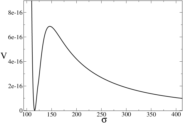
Figure 2: The uplifted potential as a function of Kähler modulus, for $r=r_{0}$ (bottom of the throat).

Having demonstrated that the minimum can be uplifted to a positive energy, we can now consider fluctuations of the brane from the bottom of the throat and show that it is indeed driven to $r=r_{0}$. We show the potential as a function of $r$ when $\sigma$ is at its minimum-energy value, in figure 3. The fact that the potential turns over and goes to zero at some value of $r$ is understandable, because of the form of the superpotential (23), which vanishes at some maximum value of $r$, for fixed angles. We have checked that this is exponentially close (of order $e^{-a\sigma}$) to the value of $r$ at which the potential shown in figure 3 vanishes. Without the competition between the superpotential and the correction (43), we do not get any uplifting effect.

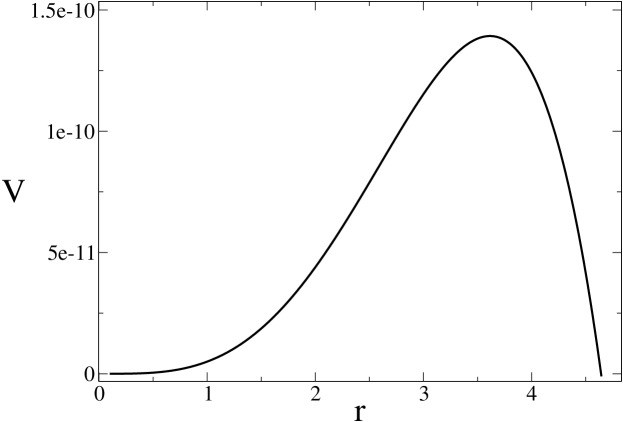
Figure 3: The potential as a function of $r$ at the stationary value of $\sigma$.

Potential near the bottom of the throat

For completeness, we note that the form of the full potential for the brane simplifies in the region $r\ll\mu^{2/3}$. In this region, $V_{O}\sim r^{4}$ while $V_{i}\sim r$ in (47-49), and we can approximate (50) by Taylor-expanding in $V_{0}$, giving

$$\sin^{2}\left(\textstyle\frac{1}{2}\theta\right)=-{V_{O}\over V_{1}}={|V_{O}|\over V_{1}}$$ (53)

This results in the potential

$$V(r) = |V_{O}|\left[1-{|V_{O}|\over V_{1}}\,\log\left({r^{3/2}\over\mu}\right)\right]+V_{\scriptscriptstyle KKLT}$$ (54)

where $V_{\scriptscriptstyle KKLT}$ depends on $r$ only weakly, $V_{\scriptscriptstyle KKLT}=-C/R^{2}$, since $R=(2\sigma-cr^{2})$ and $C$ is a positive constant. Of course this “weak” dependence was the origin of the severe $\eta$ problem of the KKLMMT model, but here the $r^{2}$ dependence is removed, because the first term in (54) is tuned to go like $C/R^{2}$ as $r\to r_{0}$, so that the potential is zero at its minimum. This causes the $r^{2}$ dependence in $R$ to be subleading to the main $r^{4}$ behavior of the potential.

3.3 Slow roll brane-antibrane inflation?

We next explore in a preliminary way whether the potential corrections considered above can be used to obtain slow roll inflation. First we consider the evolution for small $r$, where we have seen that the potential varies for small $r$ like $r^{4}$. However, the kinetic term for the inflaton is in this case given by [3, 6]

$$M_{p}^{2}{6\,c\,\sigma\over R^{2}}\,\dot{r}^{2}\sim{T_{3}\over\sigma}\dot{r}^{2}\,.$$ (55)

In the limit where $cr^{2}\ll 2\sigma$ and $R\cong 2\sigma$, this implies that the canonically normalized field, $\psi$, satisfies

$$\frac{\psi}{M_{p}}=\sqrt{3\,c\,r^{2}\over\sigma}<\sqrt{6}\,.$$ (56)

The inequality in (56) follows because $R$ can never become negative (being related to the physical size of the Calabi-Yau), and so $r$ cannot exceed $\sqrt{2\sigma/c}$.

On the other hand, in order to obtain chaotic inflation with a $\psi^{4}$ potential, one needs to ensure that the $\eta$ parameter, $M_{p}^{2}V^{\prime\prime}/V=12M_{p}^{2}/\psi^{2}$, is much smaller than unity, with inflation ending when $\eta\sim 1$ — that is, when $\psi=\sqrt{12}M_{p}$. This shows that (56) is incompatible with chaotic slow-roll inflation: the field is already rolling too fast even for the largest values of $r$.

Next, we consider whether it is possible to inflate from the top of the potential where it has a local maximum. This is equivalent to asking whether we can use the negative curvature of our new contribution to the potential to cancel the positive curvature which comes from expanding an antibrane contribution to the potential (52) in $r$. In the approximation of ignoring the brane-antibrane Coulombic attraction term, there is no difference between (52) and the KKLT potential (51) as far as their $r$-dependence is concerned.

At the local maximum of the potential shown in figure 3, the value of $\eta$ is

$$|\eta|\sim{\sigma\over c}\left|{V_{,rr}\over V}\right|\sim{\sigma\over c\,r_{m}^{2}}\gg 1$$ (57)

where $r_{m}\sim 1$ is the value of $r$ at the maximum. To obtain a smaller value of $\eta$, one should choose parameters such that $r_{m}$ becomes larger. However, the condition $R>0$ ensures that $r$ must satisfy the constraint $r<\sqrt{2\sigma/c}$, and this shows that in the best case $\eta$ can at most be of order $1$, whereas we need $\eta\sim 1/N_{e}$ with $N_{e}\sim 60$ being the number of $e$-foldings of inflation.

It is possible that slow-roll inflation might become possible in more complicated constructions, such as if supersymmetry-breaking fluxes are turned on on the D7 branes. In this case it may be possible to balance the resulting $D$-term potential, which acts to attract the D3 brane towards the D7, with the $F$-term potential considered here. We leave a more detailed study of the interplay of these D3 forces to future work.

4 Applications to orbifolds $M\times T^{2}/\Gamma$

We next specialize to toroidal geometries for which the internal geometry is locally a product of the 4-manifold, $M$, and an orbifolded 2-torus, $T^{2}/{\Gamma}$, with the various D7’s wrapping $M$ and located at the fixed points, $z=z_{s}$, of the orbifold. (In this section we denote the complex coordinates on $M$ by $y^{i}$ and those on $T^{2}/\Gamma$ by $z$, so that the coordinates on $M\times T^{2}/\Gamma$ are $\{u^{m}\}=\{y^{i},z\}$.) For instance for the case of $K3\times T^{2}/\mathbb{Z}_{2}$ we would have 4 D7’s and an orientifold plane – each of which wraps $K3$ – located at each of 4 fixed points on $T^{2}/\mathbb{Z}_{2}$. Our interest in this instance is in the motion of an itinerant D3 brane within the flat toroidal dimensions.

4.1 The gauge coupling function

The dependence of the perturbed warp factor, $h(u)$, on the D3 position, $z$, is found by solving the perturbed supergravity equations in the bulk. Taking $h\to h_{0}+\delta h$, we have

$$\tilde{\nabla}_{u}^{2}\delta h(u)=-2\kappa_{10}^{2}T_{3}\left[\frac{\delta^{6}(u-z)}{\sqrt{\tilde{g}}_{6}}-\sigma_{b}\right]\,,$$ (58)

where $\sigma_{b}$ is the background charge density coming from the adjustments made by all of the other sources in response to the presence of the D3 in order to maintain the topological condition that the integration over the left-hand-side vanish for a compact space. The authors of ref. [18] argue that the presence of the $\sigma_{b}$ term implies the existence of a nonholomorphic contribution to $\delta h$

$$e^{4u}\,\delta h=G(u^{m};z)+\overline{G}(\overline{u}^{\overline{m}};\overline{z})+\frac{\kappa_{4}^{2}T_{3}}{3}\,k(z,\overline{z})\,,$$ (59)

with the last term precisely cancelling the nonholomorphic contribution of $\delta e^{4u}$ in its contributions to the gauge coupling function. (Here $e^{u}$ represents the breathing mode, $\tilde{g}_{m\overline{n}}=e^{2u}g_{m\overline{n}}$.) The resulting gauge coupling function is then determined by the holomorphic contribution, $G(u^{m},z)$, of the appropriate Green’s function, suitably integrated over the cycle, $\Sigma$, wrapped by the corresponding D7 brane.

With these results the gauge coupling function for the D7 brane located at $z=z_{s}$ on $T^{2}/\Gamma$ becomes $f_{s}(\rho,z)=\rho+F_{a}(z)$, with the D3 position-dependence being

$$F_{s}(z) \propto {\cal T}_{7}\,\int_{\Sigma}d^{4}y\sqrt{g_{4}}\;\delta\Bigl{(}e^{4u}\,h\Bigr{)}_{hol}{}$$ (60)

$$= {\cal T}_{7}\int_{\Sigma}d^{4}y\sqrt{g_{4}}\;G(y,z_{s};z)\,.$$

The integration of the 6D Green’s function, $G(y,z)$, over the volume of the 4-cycle $\Sigma$ simply converts the result into the appropriate 2D Green’s function. That is, integrating eq. (58) over the 4-cycle and using $\tilde{\nabla}^{2}_{u}=\tilde{\nabla}^{2}_{y}+\tilde{\nabla}^{2}_{z}$ implies $\langle\delta h\rangle_{\Sigma}$ satisfies

$$\tilde{\nabla}^{2}_{z}\langle\delta h\rangle_{\Sigma}=-\frac{2\kappa_{10}^{2}T_{3}}{\tilde{V}_{\Sigma}}\left[\frac{\delta^{2}(y-z)}{\sqrt{\tilde{g}_{2}}}-\sigma_{2}\right]\,,$$ (61)

where we define $\langle\cdots\rangle_{\Sigma}=\tilde{V}_{\Sigma}^{-1}\int d^{4}y\sqrt{\tilde{g}_{4}}(\cdots)$, $\tilde{V}_{\Sigma}$ is the volume of the 4-cycle computed with the metric $\tilde{g}_{mn}$, $\tilde{\nabla}^{2}_{z}$ denotes the 2D Laplacian and $\sigma_{2}=\int_{\Sigma}d^{4}y\sqrt{\tilde{g}_{4}}\;\sigma_{b}$. For instance, for the torus defined by the lattice $y\simeq y+1\simeq y+\tau$, with complex modulus $\tau=\tau_{1}+i\tau_{2}$ and Kähler metric ${\rm d}s^{2}_{\scriptscriptstyle T}={\rm d}y\,{\rm d}\overline{y}$, the volume of the 2-torus is $V_{T}=\tau_{2}$ and $\sigma_{2}=1/\tau_{2}$. The result for $\langle\delta h\rangle_{\Sigma}$ then becomes

$$\langle\delta h(w,\overline{w})\rangle_{\Sigma}=-2\kappa_{4}^{2}T_{3}\tau_{2}\left[\frac{(w-\overline{w})^{2}}{8\tau_{2}}+\frac{1}{4\pi}\ln\Bigl{|}\vartheta_{1}\left(\pi w|\tau\right)\Bigr{|}^{2}\right]\,,$$ (62)

where $w=z-z^{\prime}$ and we use $\kappa_{10}^{2}=\kappa_{4}^{2}V_{6}=\kappa^{2}_{4}V_{\Sigma}\tau_{2}$. Again the nonholomorphic part is proportional to the 2D Kähler potential, $k(w,\overline{w})$, which ref. [18] argues is cancelled by the nonholomorphic contribution of the back-reaction to $e^{4u}$.

A similar result holds when the two dimensions transverse to the D7 are orbifolded, obtained by summing eq. (62) over the appropriate image points:

$$\langle\delta h(w,\overline{w})\rangle_{\Sigma}=-2\kappa_{4}^{2}T_{3}\tau_{2}\sum_{p}\left[\frac{(w_{p}-\overline{w}_{p})^{2}}{8\tau_{2}}+\frac{1}{4\pi}\ln\Bigl{|}\vartheta_{1}\left(\pi w_{p}|\tau\right)\Bigr{|}^{2}\right]\,,$$ (63)

where $w_{p}=z-g_{p}(z^{\prime})$ and $g_{p}(z^{\prime})$ denotes the action on the D3 brane position, $z^{\prime}$, of the discrete group elements, $g_{p}$, with the sum running over all of the elements of the group. For instance, for the orbifold $T^{2}/\mathbb{Z}_{2}$ defined by identifying points under reflection of a square torus about the origin, we have $g_{+}(z)=z$ and $g_{-}(z)=-z$ and $\tau=i$, and so $w_{+}=w=z-z^{\prime}$ while $w_{-}=z+z^{\prime}$.

Using this in expression (60) gives the following expression for the dependence of $F_{s}(z)$ on the D3 position

$$F_{s}(z)=C\sum_{p}\ln\Bigl{(}\vartheta_{1}\left[\pi(z_{s}-z_{p})|\tau\right]\Bigr{)}\,,$$ (64)

where $z$ denotes the position of the itinerant D3 brane in the orbifold, $z_{p}$ is its image under the orbifold group elements, and $z_{s}$ is the position of the D7 brane of interest. $C$ denotes a constant whose detailed form is not crucial in what follows, which is proportional to the tension of the D3.

4.2 $F$-term potential: bulk fluxes

Using this in the gaugino-condensation superpotential

$$W=W_{0}+\sum_{s}A_{s}\exp\Bigl{[}-a_{s}(\rho+F_{s}(z))\Bigr{]}\,.$$ (65)

gives the low-energy expression of the forces on the D3 due to the physics of modulus stabilization. As we discussed before, the constant $W_{0}$ appears from the $G_{3}$ given in (14), and therefore expresses the effects of supersymmetry-breaking amongst the higher-dimensional fluxes which stabilize some of the moduli, while the exponential term contains the influence of gaugino condensation (or the like) on various D7 branes, and involves the dependence on the D3 position due to the back-reaction of the D3 onto the relevant gauge coupling strengths. The quantities $A_{s}$ and $a_{s}$ (which are related to $A_{0}$ and $a$ respectively in (22) and (23) for special choices of $s$) are $z$-independent constants which are calculable given the details of the underlying physics.

Periodicity properties

For later purposes it is instructive at this point to record a subtlety regarding the periodicity properties of the above expressions under the shifts $z\to z+1$ and $z\to z+\tau$ which define the underlying torus, restricting for convenience to the case of later interest: the orbifold $T^{2}/\mathbb{Z}_{2}$, with $\mathbb{Z}_{2}$ acting as $z\to-z$. Using the periodicity properties of the Jacobi $\vartheta$-function listed in the Appendix, it can be shown that the quantities

$$f_{s}(\rho,z) = \rho+\alpha\sum_{p}\ln\Bigl{(}\vartheta_{1}\left[\pi(z_{s}-z)|\tau\right]\Bigr{)}{}$$ (66)

$$= \rho+\alpha\ln\Bigl{(}\vartheta_{1}\left[\pi(z_{s}-z)|\tau\right]\vartheta_{1}\left[\pi(z_{s}+z)|\tau\right]\Bigr{)}$$

$$\hbox{and}\qquad X = \rho+\overline{\rho}-\frac{\beta\,(z-\overline{z})^{2}}{\tau_{2}}\,,$$ (67)

are invariant under the transformations

$$z\to z+1\qquad\hbox{and}\qquad\rho\to\rho{}$$

$$z\to z+\tau\qquad\hbox{and}\qquad\rho\to\rho+2i\beta\,(2z+\tau)\,,$$ (68)

provided the real constants $\alpha$ and $\beta$ are related by $\beta=\pi\alpha$.

This shows that the $F$-term potential built from the above superpotential is appropriately periodic under shifts of the D3 position, but only if the volume modulus, $\rho$, also shifts appropriately. This coupling of the shifting of $\rho$ and $z$ due to the nonperturbative $F$-term potential shows that the D3 modulus, $z$, transforms nontrivially under the classical shift symmetry, $\rho\to\rho+i\epsilon$, which is broken by anomalies down to a discrete subgroup under which both $\rho$ and $z$ shift. This bears out the observation [41] that symmetries can require the KKLT superpotential to depend on fields other than just $\rho$, although it is interesting that the the fields which are relevant are in this case the position moduli of the itinerant D3 rather than charged multiplets living on the branes. This cancellation between shifts of $z$ and $\rho$ is also noted in ref. [29].

A novel feature of this realization of the symmetry is that it does not involve any fields beyond $\rho$ and the D3 position modulus, $z$. In particular it does not involve any charged chiral fields on the branes, such as is often assumed. In fact, in the limit that the D3 approaches the relevant D7 brane the dependence of $W$ on $z$ has a natural interpretation from the point of view of the charged fields which become part of the effective 4D field theory as the mass of the D3–D7 string states become light. This is because when the D3 is sufficiently close to the D7, the mass of these states is nonzero but small enough to be included into the low-energy 4D theory, through a contribution to the superpotential of the form

$$W_{\scriptscriptstyle M}=\frac{1}{2}\,\mu_{ij}(z)\varphi^{i}\varphi^{j}\,$$ (69)

where the dependence of $\mu_{ij}(z)$ on the D3 position, $z$, is calculable and arises because of the necessity of stretching the D3–D7 strings as the D3 position changes. Furthermore, the $U(1)$ invariance of eq. (69) ensures that $\mu_{ij}(z)$ necessarily has the right transformation property to be combined into an invariant gaugino-condensation superpotential in combination with $e^{-a\rho}$ [42], along the lines discussed in refs. [41], corresponding to what would be obtained if the charged fields were integrated out. This shows why it can be possible to achieve invariance using only the fields $z$ and $\rho$.

4.3 $D$ term potential: brane fluxes

A $D$-term potential, eqs. (9) and (10), can also be generated for these compactifications if supersymmetry-breaking magnetic fluxes are turned on on some of the D7 branes. This type of $D$-term potential arises in particular if the D3 is brought close enough to the relevant D7 that the D3-D7 string states become light enough to introduce chiral multiplets whose scalar fields carry the charge of the D7 gauge group.

If we use the form of the Kähler potential, $\kappa_{4}^{2}\partial_{\rho}K=-3/X$, and the gauge kinetic function, $f_{s}=\rho+F_{s}(z)$, suggested by eqs. (66) and (67), then $V_{D}$ becomes

$$V_{D}=\sum_{s}\frac{V_{0s}}{f_{s}+\overline{f}_{s}}\left[\frac{3\,v_{s}}{X}+{\cal D}_{s}(\varphi,\overline{\varphi})\right]^{2}\,,$$ (70)

where $X=\rho+\overline{\rho}-\beta(z-\overline{z})^{2}/\tau_{2}$, the constant $V_{0s}$ is inversely proportional to the tension of the relevant brane, as well as to the volume of the 4-cycle which it wraps. The parameter $v_{s}$ is proportional to the strength of the flux whose presence on brane ‘$s$’ breaks supersymmetry. The scalar fields, $\varphi$, here denote any light scalars which are charged under the relevant gauge group and appear in the effective 4D theory. These might include light D3–D7 string states if the D3 brane is sufficiently close to the relevant D7, but would not if the D3–D7 separation should be too great.

4.4 Uplifting

The potential (70) was proposed in ref. [28] as being a potential source of uplifting to flat or anti-de Sitter space, instead of using the supersymmetry-breaking anti-D3 brane used by KKLT. However, as noted in [28] the success of this proposal is model-dependent inasmuch as it relies on the minimum of the complete scalar potential being at a place where some of the $D$-terms are nonzero. As has since been emphasized [41], this requires at least one of the $F$-terms to also be nonzero at the relevant minimum.

Both of these features are explicitly manifest in the potential $V=V_{F}+V_{D}$, if $V_{F}$ and $V_{D}$ are computed with gaugino condensation and supersymmetric flux breaking occuring on a single D7 brane. In this case if we take an itinerant D3 brane which is far enough from the D7 then the only relevant light fields are $\rho$ and $z$ because all of the charged D3–D7 states are too massive to be included in the effective 4D theory (and so ${\cal D}_{s}(\varphi,\overline{\varphi})=0$). In the absence of a Fayet-Iliopoulos term $V_{D}=0$, and at face value $V_{F}$ as computed above is minimized (and vanishes) as the D3 moves towards the D7 on which gaugino condensation and flux breaking occurs, because the gauge kinetic function, $f_{s}$, diverges logarithmically as $z\to z_{s}$. However, in reality the effective description must change before the D3 and D7 can reach one another because of the breakdown of the approximations used (such as the necessity to include the D3–D7 states which become light in this limit).

A less trivial situation would arise if a brane configuration could be devised for which there is a $U(1)$ gauge group in the low-energy theory for which all of the charged chiral multiplets, $\varphi$, have the same sign charge. In this case the low-energy theory has a $U(1)$ anomaly, whose Green-Schwarz cancellation implies the existence of a Fayet-Iliopoulos term [43], as the following argument shows. In such a case the anomaly-cancelling mechanism implies that the 4D Lagrangian contains the term $v\int B\wedge F$, where $v$ is a constant with dimensions of mass, $F={\rm d}A$ and $B$ is the appropriate two-form potential which shifts under the action of the anomalous $U(1)$ gauge transformation. Together with the $B$-field kinetic terms, this dualizes to a Lagrangian of the form

$$S_{4dgs}=-\int d^{4}x\left[\sqrt{-g}\;\frac{1}{2}(\partial_{\mu}a-vA_{\mu})(\partial^{\mu}a-vA^{\mu})+c^{\prime}\,a\,F\wedge F\right]\,,$$ (71)

where $a$ is the Goldstone mode dual to $B_{\mu\nu}$ in four dimensions, and $c^{\prime}$ is an appropriate constant. $N=1$ supersymmetry then implies that the corresponding SUSY multiplets $A$ and $\psi$ only enter the Kähler potential of the low-energy theory through the combination $\psi+\overline{\psi}-vA$ within the Kähler function, $K$, where $\psi$ is the complex scalar whose imaginary part is $a$ and $A$ is the vector multiplet containing $A_{\mu}$. This leads to an FI term having the form $\xi=-v\partial_{\psi}K=3v/X$. Furthermore, eq. (71) requires the gauge kinetic term for $A_{\mu}$ must contain a term linear in $\psi$.

Of particular interest for us is the case where the relevant scalar $a$ is the imaginary part of the volume modulus, $\rho$, since we know that this field generically does appear linearly in the gauge kinetic functions in type IIB compactifications. Since this field comes from the component $C_{\mu\nu mn}$ of the RR 4-form field, the 4D Green-Schwarz term can be regarded as the low-energy expression of the underlying 7-brane Chern-Simons coupling

$$S_{cs}\propto\int C\wedge F\wedge{\cal F}\,,$$ (72)

where $F_{\mu\nu}$ is the 4D gauge field for the anomalous $U(1)$ and as above ${\cal F}_{mn}$ is the background flux whose SUSY-breaking presence the FI term represents.

In such a case the $D$-term potential contains contributions from both the FI term as well as the contributions of the charged scalars, ${\cal D}_{s}(\varphi,\overline{\varphi})$. However the relative sign of these contributions to $D_{s}$ is dictated by supersymmetry and anomaly cancellation, and is such that the minimization with respect to $\varphi$ cannot cancel ${\cal D}_{s}$ against the FI term, leading to a minimum at ${\cal D}_{s}=0$, with a surviving nonzero FI term available to play a role in uplifting. It would clearly be of considerable interest to realize this picture within a bona fide string construction.

4.5 Beyond linear backreaction?

The derivation leading to eqs. (6), (24) and (70) for the potentials $V_{F}$ and $V_{D}$, includes the D3-brane position through its dependence on the gauge kinetic function, $f_{s}=\rho+F_{s}$, and on the Kähler variable, $X$, which themselves depend on the D3 position through eqs. (59) and (19) (or (67)). This dependence arises due to the back-reaction on the bulk fields of the D3 position, and was computed by linearizing about the D3-independent background. This leads us to ask whether the domain of validity of the 4D potential must also be restricted to linear order in $F$ and $\delta X=X-\rho-\overline{\rho}$.

Part of the virtue of having a formulation in terms of 4D supergravity lies in the various nonrenormalization theorems which such theories enjoy [44, 45]. For holomorphic quantities like the gauge kinetic function and superpotential, these theorems often allow the extension of nominally low-order results beyond the domain of their initial derivation. In particular, since nonrenormalization theorems often restrict the corrections to the gauge kinetic function to arise only at lowest order, we expect that it may be a good approximation to keep the full dependence of $f_{s}=\rho+F_{s}$ on $z$, without having to linearize results to lowest order in $F$.

Similar arguments are more difficult to make for $X$, however, since corrections to the Kähler function of the low-energy 4D supergravity are typically not protected from receiving perturbative corrections. Indeed, it can happen that interesting and qualitatively new kinds of minima actually do arise for the scalar potential once the leading such corrections are taken into account [46].

5 Conclusions

Building on the work of [18], we have shown that the KKLT stabilization mechanism, with the addition of a mobile D3 brane, necessarily involves extra superpotential and dilaton background corrections. These are a consequence of the same mechanism that stabilizes the Kähler modulus, either Euclidean D3 branes or gaugino condensation. In a scenario like brane-antibrane inflation where D3 branes are involved it is necessary to add these corrections.

The new corrections depend upon which 4-cycle in the KS-throat is wrapped by the D7 brane, or stack of D7 branes. In the present work we have focused on a particularly simple choice of 4-cycle, and the case of a single D7 brane. Our preliminary study of other choices indicate that they have similar qualitative behavior to the simple case we studied.

A major motivation for studying this system was to determine whether the superpotential correction can be fine-tuned to ameliorate the $\eta$ problem of brane-antibrane slow roll inflation à la KKLMMT [3]. A yet more fortunate outcome would have been to find that our potential supports slow roll inflation by itself, even without an antibrane. We found that neither of these possibilities could be realized. Either one would have required large values of $r$, inconsistent with the requirement $cr^{2}\ll 2\sigma$, needed in order to keep the volume of the extra dimensions sufficiently large that the low-energy effective description can be trusted. It has been suggested that these problems can be overcome in a more elaborate related background, the full resolved warped deformed conifold [40], although it would be worth extending their analysis to a case for which all moduli are stabilized.

Finally, we examine a simple toroidal example and exhibit the $F$ and $D$ term potentials which express in the low-energy 4D theory various forces on a mobile D3 brane. We show how the D3 position modulus can play the role of the field which ensures the invariance of the superpotential under otherwise-puzzling symmetries. We imagine the resulting potential could be useful for exploring D3–D7 inflationary models in more detail.

Appendix A Theta functions

We record in this appendix some of the properties of the Jacobi $\vartheta$-functions we use in the main text. We use the definition

$$\vartheta_{1}(z|\tau) = -i\sum_{n=-\infty}^{\infty}(-)^{n}q^{\left(n+\frac{1}{2}\right)^{2}}\,e^{i(2n+1)z}{}$$ (73)

$$= 2\sum_{n=0}^{\infty}(-)^{n}q^{\left(n+\frac{1}{2}\right)^{2}}\sin\Bigl{[}(2n+1)z\Bigr{]}\,,$$

where $q=e^{i\pi\tau}$. This definition ensures that $\vartheta_{1}(-z|\tau)=-\vartheta_{1}(z|\tau)$, as well as the toroidal periodicity properties

$$\vartheta_{1}(z+n\pi|\tau) = (-)^{n}\vartheta_{1}(z|\tau){}$$

$$\hbox{and}\quad\vartheta_{1}(z-n\pi\tau|\tau) = (-)^{n}q^{-n^{2}}e^{2niz}\vartheta_{1}(z|\tau)\,,$$ (74)

for any integer $n$. Similarly, the identity

$$\frac{\vartheta^{\prime}_{1}(z|\tau)}{\vartheta_{1}(z|\tau)}=\cot z+4\sum_{n=1}^{\infty}\left(\frac{q^{2n}}{1-q^{2n}}\right)\sin(2nz)\,,$$ (75)

where $\vartheta^{\prime}_{1}(z|\tau)={\rm d}\vartheta_{1}(z|\tau)/{\rm d}z$, implies that near $z=0$ we have $\vartheta_{1}(z|\tau)=z+O(z^{3})$.

Appendix B 4D anomaly cancellation

In this appendix we confirm the relative sign between the contributions to the $D$-terms from the Fayet-Iliopoulos (FI) term and from the charged matter multiplets. We show that in the special case where all of the matter multiplets share the same charge the resulting potential is minimized by having the charged scalars vanish, leaving the D3 dynamics governed by the FI term, as argued in ref. [28].

We start with the 4D $U(1)$ anomaly due to a collection of fermions, all of which carry the same $U(1)$ charge $q$. By an appropriate choice of counterterms the variation of the quantum action under such an anomaly can be written in the form:

$$\delta S=\frac{Aq}{16\pi^{2}}\int{\rm d}^{4}x\,\omega\epsilon^{\mu\nu\lambda\rho}F_{\mu\nu}F_{\lambda\rho}\,,$$ (76)

where $\omega$ is the $U(1)$ symmetry transformation parameters and $A$ is a positive calculable constant.

Within the 4D Green-Schwarz mechanism this anomaly is cancelled by the presence of a local interaction, given the presence of a 2-form gauge potential, $B_{\mu\nu}$, with an action

$$S_{\scriptscriptstyle GS}=-\int{\rm d}^{4}x\left[\frac{1}{12}\,\sqrt{-g}\,H^{\mu\nu\lambda}H_{\mu\nu\lambda}+k\epsilon^{\mu\nu\lambda\rho}B_{\mu\nu}F_{\lambda\rho}\right]\,,$$ (77)

where the field strength

$$H_{\mu\nu\lambda}=\partial_{\mu}B_{\nu\lambda}-\kappa A_{\mu}F_{\nu\lambda}+\hbox{cyclic}\,,$$ (78)

is invariant under the following $U(1)$ gauge transformations

$$\delta A_{\mu}=\partial_{\mu}\omega\qquad\hbox{and}\qquad\delta B_{\mu\nu}=\omega\kappa F_{\mu\nu}\,,$$ (79)

and $\kappa$ is a positive dimensionful constant. This action cancels the anomaly for an appropriate choice of $k$ because its variation under the $U(1)$ transformation is

$$\delta S_{\scriptscriptstyle GS}=-\kappa k\int{\rm d}^{4}x\;\omega\epsilon^{\mu\nu\lambda\rho}F_{\mu\nu}F_{\lambda\rho}\,.$$ (80)

This cancels the fermionic anomaly provided $\kappa k=Aq/(16\pi^{2})$.

The connection to supersymmetric $D$-terms is best seen once the 2-form field is dualized, leading in 4D to a scalar field, $a$. This duality is most easily performed by rewriting the Green-Schwarz action as

$$S_{\scriptscriptstyle GS} = -\int{\rm d}^{4}x\left[\frac{1}{12}\,\sqrt{-g}\,H^{\mu\nu\lambda}H_{\mu\nu\lambda}+\frac{2k}{3}\epsilon^{\mu\nu\lambda\rho}A_{\mu}H_{\nu\lambda\rho}\right.{}$$ (81)

$$\qquad\qquad\qquad\qquad\qquad\left.+\frac{1}{6}\,a\,\epsilon^{\mu\nu\lambda\rho}\left(\partial_{\mu}H_{\nu\lambda\rho}+\frac{3\kappa}{2}F_{\mu\nu}F_{\lambda\rho}\right)\right]\,,$$

and regarding the functional integral to be over the fields $H_{\mu\nu\lambda}$ and $a$, rather than $B_{\mu\nu}$. The equivalence of this form with eq. (77) is seen by performing the functional integral over the field $a$, which acts as a Lagrange multiplier enforcing the Bianchi identity:

$$\epsilon^{\mu\nu\lambda\rho}\partial_{\mu}H_{\nu\lambda\rho}=-\frac{3\kappa}{2}\epsilon^{\mu\nu\lambda\rho}F_{\mu\nu}F_{\lambda\rho}\,.$$ (82)

This has eq. (78) as its local solution, allowing the functional integral over $H_{\mu\nu\lambda}$ to be traded for an integral over $B_{\mu\nu}$, weighted by the action (77).

The dual formulation is obtained by performing the functional integrals in the opposite order, first integrating over $H_{\mu\nu\lambda}$ to leave an action in terms of the scalar field $a$. Since the integral over $H_{\mu\nu\lambda}$ is Gaussian, it may be performed explicitly, leading to the saddle point $H_{\mu\nu\lambda}=-\epsilon_{\mu\nu\lambda\rho}D^{\rho}a$, where the covariant derivative

$$D_{\mu}a=\partial_{\mu}a-4k\,A_{\mu}\,,$$ (83)

is invariant under the $U(1)$ transformations

$$\delta A_{\mu}=\partial_{\mu}\omega\qquad\hbox{and}\qquad\delta a=4k\omega\,.$$ (84)

The resulting dual action for $a$ then becomes:

$$\tilde{S}_{\scriptscriptstyle GS}=-\int{\rm d}^{4}x\;\left[\frac{1}{2}\,D_{\mu}aD^{\mu}a+\frac{\kappa}{4}\,a\,\epsilon^{\mu\nu\lambda\rho}F_{\mu\nu}F_{\lambda\rho}\right]\,,$$ (85)

which again reproduces the proper anomalous $U(1)$ transformation.

Within a 4D $N=1$ supersymmetric context the ‘constants’ $k$ and $\kappa$ typically depend on various moduli fields, but the above arguments carry through basically unchanged. In this case the scalar $a$ resides within a complex chiral scalar multiplet, $\rho=\kappa(z+2ia)$, and so the second term in the action (85) requires $\rho$ to appear linearly in the holomorphic gauge kinetic function: $f=\rho+\cdots$, and so

$$S_{g}=-\frac{1}{4}\int{\rm d}^{4}x\;\Bigl{[}\sqrt{-g}\;\kappa\,z\,F_{\mu\nu}F^{\mu\nu}+\kappa a\epsilon^{\mu\nu\lambda\rho}F_{\mu\nu}F_{\lambda\rho}\Bigr{]}\,.$$ (86)

By contrast, the kinetic term for $a$ and for the charged matter fields, $\varphi$, arise from the Kähler function $K=K_{1}(\rho+\overline{\rho}+cV)+K_{2}(\overline{\varphi}e^{qV},\varphi)$, where $V$ denotes the $U(1)$ gauge multiplet and $c=-4\kappa k=-Aq/(4\pi^{2})$ is required in order to ensure that $\partial_{\mu}a$ and $A_{\mu}$ only appear through the invariant combination $D_{\mu}a=\partial_{\mu}a-4kA_{\mu}$. The Kähler function is also the source of the $D$-term contributions

$$\left[\left(c\,\frac{\partial K_{1}}{\partial\rho}+q\overline{\varphi}\frac{\partial K_{2}}{\partial\overline{\varphi}}\right)_{V=0}\,V\right]_{D}=q\left(-\frac{A}{4\pi^{2}}\,\frac{\partial K_{1}}{\partial\rho}+\overline{\varphi}\frac{\partial K_{2}}{\partial\overline{\varphi}}\right)_{V=0}D\,.$$ (87)

which show that the relative size of the two contributions is independent of the sign of $q$. In particular, using $\kappa^{2}K_{1}=-3\ln(\rho+\overline{\rho})$ and the ‘minimal’ choice, $K_{2}=\overline{\varphi}e^{qV}\varphi$, implies

$$D\propto q\left(\frac{3A}{4\pi^{2}\kappa^{2}(\rho+\overline{\rho})}+\overline{\varphi}\varphi\right)\,,$$ (88)

in agreement with refs. [41]. Clearly, in the absence of any other $\varphi$-dependence, the $D$-term potential $V_{D}\propto D^{2}$ is minimized by $\varphi=0$ because of the conditions that $\kappa^{2}(\rho+\overline{\rho})/A$ is positive.

References

- [1] G. R. Dvali and S. H. H. Tye, “Brane inflation,” Phys. Lett. B 450 (1999) 72 [hep-ph/9812483]; S. H. S. Alexander, “Inflation from D - anti-D brane annihilation,” Phys. Rev. D 65, 023507 (2002) [hep-th/0105032].
- [2] C. P. Burgess, M. Majumdar, D. Nolte, F. Quevedo, G. Rajesh and R. J. Zhang, “The inflationary brane-antibrane universe,” JHEP 0107 (2001) 047 [hep-th/0105204]. G. R. Dvali, Q. Shafi and S. Solganik, “D-brane inflation,” hep-th/0105203.
- [3] S. Kachru, R. Kallosh, A. Linde, J. Maldacena, L. McAllister and S. P. Trivedi, “Towards inflation in string theory,” JCAP 0310 (2003) 013 [hep-th/0308055].
- [4] J. Garcia-Bellido, R. Rabadan and F. Zamora, “Inflationary scenarios from branes at angles,” JHEP 0201, 036 (2002); N. Jones, H. Stoica and S. H. H. Tye, “Brane interaction as the origin of inflation,” JHEP 0207, 051 (2002); M. Gomez-Reino and I. Zavala, JHEP 0209, 020 (2002).
- [5] H. Firouzjahi and S. H. Tye, “Closer towards inflation in string theory,” Phys. Lett. B 584 (2004) 147 [hep-th/0312020]; S.E. Shandera and S.H. Tye, “Observing Brane Inflation,” [hep-th/0601099].
- [6] C. P. Burgess, J. M. Cline, H. Stoica and F. Quevedo, “Inflation in realistic D-brane models,” JHEP 0409, 033 (2004) [hep-th/0403119]; J. M. Cline and H. Stoica, “Multibrane inflation and dynamical flattening of the inflaton potential,” Phys. Rev. D 72, 126004 (2005) [hep-th/0508029].
- [7] K. Dasgupta, C. Herdeiro, S. Hirano and R. Kallosh, “D3/D7 inflationary model and M-theory,” Phys. Rev. D 65, 126002 (2002) [hep-th/0203019]; K. Dasgupta, J. P. Hsu, R. Kallosh, A. Linde and M. Zagermann, “D3/D7 brane inflation and semilocal strings,” JHEP 0408, 030 (2004) [hep-th/0405247]; P. Chen, K. Dasgupta, K. Narayan, M. Shmakova and M. Zagermann, “Brane inflation, solitons and cosmological solutions: I,” JHEP 0509, 009 (2005) [hep-th/0501185].
- [8] J. P. Hsu, R. Kallosh and S. Prokushkin, “On brane inflation with volume stabilization,” JCAP 0312 (2003) 009 [hep-th/0311077]; F. Koyama, Y. Tachikawa and T. Watari, “Supergravity analysis of hybrid inflation model from D3-D7 system”, [hep-th/0311191]; J. P. Hsu and R. Kallosh, “Volume stabilization and the origin of the inflaton shift symmetry in string theory,” JHEP 0404 (2004) 042 [hep-th/0402047];
- [9] C. P. Burgess, P. Martineau, F. Quevedo, G. Rajesh and R. J. Zhang, “Brane antibrane inflation in orbifold and orientifold models,” JHEP 0203 (2002) 052 [hep-th/0111025]; J. J. Blanco-Pillado et al., “Racetrack inflation,” JHEP 0411 (2004) 063 [hep-th/0406230]; Z. Lalak, G. G. Ross and S. Sarkar, “Racetrack inflation and assisted moduli stabilisation,” [hep-th/0503178]; J. P. Conlon and F. Quevedo, “Kähler moduli inflation,” JHEP 0601 (2006) 146 [hep-th/0509012]; J. J. Blanco-Pillado et al., “Inflating in a better racetrack,” [hep-th/0603129].
- [10] E. Silverstein and D. Tong, “Scalar speed limits and cosmology: Acceleration from D-cceleration,” Phys. Rev. D 70 (2004) 103505 [hep-th/0310221]; M. Alishahiha, E. Silverstein and D. Tong, “DBI in the sky,” Phys. Rev. D 70 (2004) 123505 [hep-th/0404084]; X. G. Chen, “Inflation from warped space,” JHEP 0508 (2005) 045 [hep-th/0501184]; “Running non-Gaussianities in DBI inflation,” [astro-ph/0507053]; D. Cremades, F. Quevedo and A. Sinha, “Warped tachyonic inflation in type IIB flux compactifications and the open-string completeness conjecture,” JHEP 0510 (2005) 106 [hep-th/0505252].
- [11] O. DeWolfe, S. Kachru and H. Verlinde, “The giant inflaton,” JHEP 0405 (2004) 017 [hep-th/0403123]; N. Iizuka and S. P. Trivedi, “An inflationary model in string theory,” [hep-th/0403203]; B. Freivogel, V. E. Hubeny, A. Maloney, R. Myers, M. Rangamani and S. Shenker, “Inflation in AdS/CFT,” JHEP 0603 (2006) 007 [hep-th/0510046]; S. Dimopoulos, S. Kachru, J. McGreevy and J. G. Wacker, “N-flation,” [hep-th/0507205]; K. Becker, M. Becker and A. Krause, Nucl. Phys. B715 (2005) 349-371 [hep-th/0501130]; [hep-th/0510066].
- [12] K. Maeda and N. Ohta, “Inflation from M-theory with fourth-order corrections and large extra dimensions,” Phys. Lett. B 597 (2004) 400 [hep-th/0405205]; “Inflation from superstring / M theory compactification with higher order corrections. I,” Phys. Rev. D 71 (2005) 063520 [hep-th/0411093]; K. Akune, K. Maeda and N. Ohta, “Inflation from superstring / M-theory compactification with higher order corrections. II: Case of quartic Weyl terms,” Phys. Rev. D 73 (2006) 103506 [hep-th/0602242]; N. Ohta, “Accelerating cosmologies and inflation from M / superstring theories,” Int. J. Mod. Phys. A 20 (2005) 1 [hep-th/0411230].
- [13] S. B. Giddings, S. Kachru and J. Polchinski, “Hierarchies from fluxes in string compactifications,” Phys. Rev. D66, 106006 (2002) [hep-th/0105097].
- [14] S. Sethi, C. Vafa and E. Witten, “Constraints on low-dimensional string compactifications,” Nucl. Phys. B 480 (1996) 213 [hep-th/9606122]; K. Dasgupta, G. Rajesh and S. Sethi, “M theory, orientifolds and G-flux,” JHEP 9908 (1999) 023 [hep-th/9908088].
- [15] S. Kachru, R. Kallosh, A. Linde and S. P. Trivedi, “de Sitter Vacua in String Theory,” Phys. Rev. D 68 (2003) 046005 [hep-th/0301240]; B. S. Acharya, “A moduli fixing mechanism in M theory,” [hep-th/0212294]; R. Brustein and S. P. de Alwis, “Moduli potentials in string compactifications with fluxes: Mapping the discretuum,” Phys. Rev. D 69 (2004) 126006 [hep-th/0402088].
- [16] F. Denef, M. R. Douglas and B. Florea, “Building a better racetrack,” JHEP 0406 (2004) 034 [hep-th/0404257]; F. Denef, M. R. Douglas, B. Florea, A. Grassi and S. Kachru, “Fixing all moduli in a simple F-theory compactification,” [hep-th/0503124].
- [17] J. M. Cornwall, D. N. Levin and G. Tiktopoulos, “Derivation Of Gauge Invariance From High-Energy Unitarity Bounds On The S - Matrix,” Phys. Rev. D 10, 1145 (1974) [Erratum-ibid. D 11, 972 (1975)]; M.S. Chanowitz, M. Golden and H. Georgi, Phys. Rev. D 36 (1987) 1490; C. P. Burgess and D. London, “On anomalous gauge boson couplings and loop calculations,” Phys. Rev. Lett. 69 (1992) 3428; Phys. Rev. D 48 (1993) 4337 [hep-ph/9203216].
- [18] D. Baumann, A. Dymarsky, I. R. Klebanov, J. Maldacena, L. McAllister and A. Murugan, “On D3-brane potentials in compactifications with fluxes and wrapped D-branes,” hep-th/0607050.
- [19] K. Dasgupta and S. Mukhi, “F-theory at constant coupling,” Phys. Lett. B 385, 125 (1996) [arXiv:hep-th/9606044].
- [20] M. Berg, M. Haack and B. Körs, “Loop corrections to volume moduli and inflation in string theory,” Phys. Rev. D71 026005 (2005) [hep-th/0404087]; M. Berg, M. Haack and B. Körs, “String loop corrections to Kähler potentials in orientifolds,” JHEP 0511 030 (2005) [hep-th/0508043].
- [21] E. Witten, “Non-Perturbative Superpotentials In String Theory,” Nucl. Phys. B 474, 343 (1996) [hep-th/9604030].
- [22] J. P. Derendinger, L. E. Ibáñez and H. P. Nilles, “On The Low-Energy D = 4, N=1 Supergravity Theory Extracted From The D = 10, N=1 Superstring,” Phys. Lett. B 155 (1985) 65; M. Dine, R. Rohm, N. Seiberg and E. Witten, “Gluino Condensation In Superstring Models,” Phys. Lett. B 156 (1985) 55; C.P. Burgess, J.-P. Derendinger, F. Quevedo and M. Quirós, “Gaugino Condensates and Chiral-Linear Duality: An Effective-Lagrangian Analysis”, Phys. Lett. B 348 (1995) 428–442; “On Gaugino Condensation with Field-Dependent Gauge Couplings”, Ann. Phys. 250 (1996) 193-233.
- [23] I. R. Klebanov and E. Witten, “AdS/CFT correspondence and symmetry breaking,” Nucl. Phys. B 556, 89 (1999) [hep-th/9905104].
- [24] I. R. Klebanov and M. J. Strassler, “Supergravity and a confining gauge theory: Duality cascades and SB-resolution of naked singularities,” JHEP 0008, 052 (2000) [hep-th/0007191].
- [25] P. Ouyang, “Holomorphic D7-Branes And Flavored N = 1 Gauge Theories,” Nucl. Phys. B 699 (2004) 207 [hep-th/0311084].
- [26] I. Brunner, M. R. Douglas, A. E. Lawrence and C. Romelsberger, “D-branes on the quintic,” JHEP 0008 (2000) 015 [hep-th/9906200]; M. Mihailescu, I. Y. Park and T. A. Tran, “D-branes as solitons of an N = 1, D = 10 non-commutative gauge theory,” Phys. Rev. D 64 (2001) 046006 [hep-th/0011079]; E. Witten, “BPS bound states of D0-D6 and D0-D8 systems in a B-field,” JHEP 0204 (2002) 012 [hep-th/0012054]; S. Kachru and J. McGreevy, “Supersymmetric three-cycles and (super)symmetry breaking,” Phys. Rev. D 61 (2000) 026001 [hep-th/9908135]; R. Blumenhagen, D. Lüst and T. R. Taylor, “Moduli stabilization in chiral type IIB orientifold models with fluxes,” Nucl. Phys. B 663 (2003) 319 [hep-th/0303016]; J. F. Cascales and A. M. Uranga, “Chiral 4d N = 1 string vacua with D-branes and NSNS and RR fluxes,” JHEP 0305 (2003) 011 [hep-th/0303024].
- [27] For T-dual versions see for instance: R. Blumenhagen, L. Goerlich, B. Kors and D. Lust, “Noncommutative compactifications of type I strings on tori with magnetic background flux,” JHEP 0010 (2000) 006 [hep-th/0007024]; G. Aldazabal, S. Franco, L. E. Ibanez, R. Rabadan and A. M. Uranga, “Intersecting brane worlds,” JHEP 0102 (2001) 047 [hep-ph/0011132]; M. Cvetic, G. Shiu and A. M. Uranga, “Chiral four-dimensional N = 1 supersymmetric type IIA orientifolds from intersecting D6-branes,” Nucl. Phys. B 615 (2001) 3 [hep-th/0107166]; D. Cremades, L. E. Ibanez and F. Marchesano, “Intersecting brane models of particle physics and the Higgs mechanism,” JHEP 0207 (2002) 022 [hep-th/0203160]; “SUSY quivers, intersecting branes and the modest hierarchy problem,” JHEP 0207 (2002) 009 [hep-th/0201205].
- [28] C. P. Burgess, R. Kallosh and F. Quevedo, “de Sitter string vacua from supersymmetric D-terms,” JHEP 0310 (2003) 056 [hep-th/0309187].
- [29] M. Haack, D. Krefl, D. Lüst, A. Van Proeyen and M. Zagermann, “Gaugino Condensates and D-terms from D7-branes,” [hep-th/0609211].
- [30] P. Fayet, J. Iliopoulos, “ Spontaneously Broken Supergauge Symmetries And Goldstone Spinors,” Phys. Lett. B 51 (1974) 461.
- [31] I. R. Klebanov and A. A. Tseytlin, “Gravity duals of supersymmetric SU(N) x SU(N+M) gauge theories,” Nucl. Phys. B 578, 123 (2000) [arXiv:hep-th/0002159].
- [32] M. Becker, K. Dasgupta, A. Knauf and R. Tatar, “Geometric transitions, flops and non-Kaehler manifolds. I,” Nucl. Phys. B 702, 207 (2004) [arXiv:hep-th/0403288]; S. Alexander, K. Becker, M. Becker, K. Dasgupta, A. Knauf and R. Tatar, “In the realm of the geometric transitions,” Nucl. Phys. B 704, 231 (2005) [arXiv:hep-th/0408192]; M. Becker, K. Dasgupta, S. H. Katz, A. Knauf and R. Tatar, “Geometric transitions, flops and non-Kaehler manifolds. II,” Nucl. Phys. B 738, 124 (2006) [arXiv:hep-th/0511099]; K. Dasgupta, M. Grisaru, R. Gwyn, S. H. Katz, A. Knauf and R. Tatar, “Gauge - gravity dualities, dipoles and new non-Kaehler manifolds,” [arXiv:hep-th/0605201]; K. Dasgupta, J. Guffin, R. Gwyn and S. H. Katz, “Dipole-deformed bound states and heterotic kodaira surfaces,” [arXiv:hep-th/0610001].
- [33] A. Butti, M. Grana, R. Minasian, M. Petrini and A. Zaffaroni, “The baryonic branch of Klebanov-Strassler solution: A supersymmetric family of SU(3) structure backgrounds,” JHEP 0503, 069 (2005) [arXiv:hep-th/0412187].
- [34] G. Papadopoulos and A. A. Tseytlin, “Complex geometry of conifolds and 5-brane wrapped on 2-sphere,” Class. Quant. Grav. 18, 1333 (2001) [arXiv:hep-th/0012034].
- [35] M. Cvetic, G. W. Gibbons, H. Lu and C. N. Pope, “Ricci-flat metrics, harmonic forms and brane resolutions,” Commun. Math. Phys. 232, 457 (2003) [arXiv:hep-th/0012011].
- [36] O. DeWolfe and S. B. Giddings, “Scales and hierarchies in warped compactifications and brane worlds,” Phys. Rev. D 67, 066008 (2003) [hep-th/0208123].
- [37] E. Cremmer, S. Ferrara, C. Kounnas and D.V. Nanonpoulos, “Naturally vanishing cosmological constant in supergravity,” Phys. Lett. B133, 61 (1983); J. Ellis, A.B. Lahanas, D.V. Nanopoulos and K. Tamvakis, “No-scale Supersymmetric Standard Model,” Phys. Lett. B134, 429 (1984).
- [38] P. Candelas and X. C. de la Ossa, “Comments on conifolds,” Nucl. Phys. B 342, 246 (1990).
- [39] K. Higashijima, T. Kimura and M. Nitta, “Supersymmetric nonlinear sigma models on Ricci-flat Kaehler manifolds with O(N) symmetry,” Phys. Lett. B 515, 421 (2001) [hep-th/0104184].
- [40] A. Dymarsky, I. R. Klebanov and N. Seiberg, “On the moduli space of the cascading SU(M+p) x SU(p) gauge theory,” JHEP 0601, 155 (2006) [hep-th/0511254].
- [41] K. Choi, A. Falkowski, H.P. Nilles and M. Olechowski, “Soft supersymmetry breaking in KKLT flux compactification,” Nucl. Phys. B718 (2005) 113 [hep-th/0503216]; S.P. de Alwis, “Effective potentials for light moduli,” Phys. Lett. B626 (2005) 223 [hep-th/0506266]; G. Villadoro and F. Zwirner, “de Sitter vacua via consistent D-terms,” Phys. Rev. Lett. 95 (2005) 231602 [hep-th/0508167]; A. Achucarro, B. de Carlos, J.A. Casas and L. Doplicher, “de Sitter vacua from uplifting D-terms in effective supergravities from realistic strings,” JHEP 0606, 014 (2006) [hep-th/0601190]; G. Villadoro and F. Zwirner, “D terms from D-branes, gauge invariance and moduli stabilization in flux compactifications,” JHEP 0603 (2006) 087 [hep-th/0602120]; Ph. Brax, C. . v. de Bruck, A. C. Davis, S. C. Davis, R. Jeannerot and M. Postma, “Moduli corrections to D-term inflation,” [hep-th/0610195].
- [42] K. A. Intriligator and N. Seiberg, “Lectures on supersymmetric gauge theories and electric-magnetic duality,” Nucl. Phys. Proc. Suppl. 45BC (1996) 1 [hep-th/9509066].
- [43] M. Dine, N. Seiberg and E. Witten, “Fayet-Iliopoulos Terms In String Theory,” Nucl. Phys. B 289 (1987) 589.
- [44] M. T. Grisaru, W. Siegel and M. Rocek, “Improved Methods For Supergraphs,” Nucl. Phys. B 159 (1979) 429; E. Witten, “New Issues In Manifolds Of SU(3) Holonomy,” Nucl. Phys. B 268 (1986) 79; M. Dine, N. Seiberg, “Nonrenormalization Theorems in Superstring Theory,” Phys. Rev. Lett. 57 (1986) 21; N. Seiberg, “Naturalness versus supersymmetric nonrenormalization theorems,” Phys. Lett. B 318 (1993) 469 [hep-ph/9309335]; C.P. Burgess, C. Escoda and F. Quevedo, “Nonrenormalization of Flux Superpotentials in String Theory,” JHEP (to appear), [hep-th/0510213].
-
[45]
Other references in which these symmetry arguments are given;
S. Weinberg, The Quantum Theory of Fields III, Cambridge University Press (1996); C. P. Burgess, A. Font and F. Quevedo, “Low-Energy Effective Action For The Superstring,” Nucl. Phys. B 272 (1986) 661; C.P. Burgess, J.P. Derendinger and F. Quevedo and M. Quiros,, Ann. Phys. 250 (1996) 193 [hep-th/9505171]; Phys. Lett. B348 (1995) 428, [hep-th/9501065]. - [46] V. Balasubramanian, P. Berglund, J. P. Conlon and F. Quevedo, “Systematics of moduli stabilisation in Calabi-Yau flux compactifications,” JHEP 0503, 007 (2005) [arXiv:hep-th/0502058].