The box diagram in Yukawa theory

Abstract

We present a light-front calculation of the box diagram in Yukawa theory. The covariant box diagram is finite for the case of spin-1/2 constituents exchanging spin-0 particles. In light-front dynamics, however, individual time-ordered diagrams are divergent. We analyze the corresponding light-front singularities and show the equivalence between the light-front and covariant results by taming the singularities.

I Introduction

One of the important theoretical tools to study relativistic bound-state problems is the light-front quantization method which provides one of the three forms Dirac of Hamiltonian dynamics and a Fock-state representation at equal light-front time $\tau=t+z/c$ BPP . Distinguished features of light-front dynamics (LFD) may be summarized in two fundamental areas of physics, namely the vacuum and symmetry in Minkowski space. Except for zero-modes, the vacuum of LFD is much simpler than the vacuum of instant form dynamics (IFD) based on the ordinary equal $t$ quantization. The rational energy-momentum dispersion relation in LFD may be the key to understand this highly non-trivial property of the vacuum. The number of kinematic generators for the Poincaré symmetry is also maximal in LFD and the conversion of dynamical generators from the boost to the transverse rotation occurs upon the replacement of IFD by LFD JM . The compact nature of the rotation may be regarded as an advantageous property of the LFD in handling complicated dynamical operators JKM .

The momentum-space bound-state solutions to a system of relativistic equations $\psi(x,{\vec{k}}_{\perp},\lambda)$ are functions of the light-front variables $x_{i}=(k^{0}_{i}+k_{i}^{z})/(p^{0}+p^{z})$, ${\vec{k}}_{\perp i}$, and the particle helicities $\lambda_{i}$. They are suitable for the calculation of physical observables such as hadron form factors and structure functions. The first step in solving the full set of coupled Fock-state equations on the light-front (LF) is to find a simple analytically tractable equation for the valence, lowest-particle-number sector, and to develop a systematic scheme of obtaining the contributions from the higher-particle-number sectors with a desired accuracy. A frequently used technique to achieve at least the first step is the projection of the manifestly covariant Bethe-Salpeter equation on the hypersurface of LFD BJS . For instance, the the LF ladder approximation can be obtained by projecting the ladder approximation of the Bethe-Salpeter equation. The ladder approximation to the LF two-body bound-state equation involves only up to three-body Fock-states and the higher-particle-number sectors beyond the three-body Fock-states cannot be generated in this approximation. However, they can be generated if the projection procedure is applied after the covariant Bethe-Salpeter equation is iterated once. As an example, the four-body Fock-state of the stretched box diagram in LFD can be generated by projecting the covariant box diagram after iterating once the ladder kernel of the Bethe-Salpeter equation. In this sense, the procedures of iteration and projection do not commute.

A three-dimensional reduction of the two-particle Bethe-Salpeter equation has been proposed SFCS2000 and the reduction of the two-fermion Bethe-Salpeter equation in the framework of LFD has been studied for the 3+1 dimensional Yukawa model SFCS2001 . We study here a generalization of this model for which the interaction Lagrangian density is given by

$$L=g_{1}{\bar{\Psi}}_{1}\Psi_{1}\phi_{1}+g_{2}{\bar{\Psi}}_{2}\Psi_{2}\phi_{2},+g_{12}({\bar{\Psi}}_{1}\Psi_{2}\sigma+{\rm h.c.}),$$ (1)

where the fermions correspond to the fields $\Psi_{1,2}$ with rest masses $M,\;m$ and the exchanged bosons to the fields $\phi_{1}$, $\phi_{2}$, and $\sigma$ with masses $\mu_{1}$, $\mu_{2}$, and $\mu$, respectively. A physical system where this interaction would be applicable is the coupled $NN-N^{*}N^{*}$ system.

The LF treatment yields three-dimensional quantities for the transition matrix and the bound-state wave function. Since the kernel of the LF Tamm-Dancoff PHW reduced Bethe-Salpeter equation for the vertex function for the one-boson-exchange interaction in ladder approximation has a divergence problem, the introduction of a counterterm to renormalize the integral equation was proposed GHPSW . In Ref. SFCS2001 , the authors were concerned with the origin of the perturbative counterterms of the LF ladder Bethe-Salpeter equation for the Yukawa model and showed that the kernel of the auxiliary integral equation, expanded up to the fourth power of the coupling constant, $g^{4}$, naturally yielded the box counterterm GHPSW and a well defined finite part. As the authors explained, this is because the perturbative expansion of the LF scattering amplitude in powers of the coupling constant, obtained from the LF $T$-matrix equation with the kernel calculated up to the same order, necessarily reproduces the perturbative covariant ladder scattering amplitude at that order in $g$. An important necessary inclusion, in addition to the instantaneous contributions, is the higher Fock components by going beyond the Tamm-Dancoff approximation. For example, in Ref. SFCS2001 , the divergence could not be removed if the four-body Fock-component represented by the simultaneous propagation of two $\sigma$s and two fermions occuring between the creation and annihilation of the bosons was not included. Even higher Fock-state contributions such as the simultaneous propagation of three $\sigma$s and two fermions should be necessary if terms of order $g^{6}$ are included in the kernel. Such a requirement of including higher Fock-state contributions to remove the relevant divergence in LFD would persist if higher and higher Fock sectors would be included. Thus, it is not clear how the reduction program would work in practice even if the expansion in powers of the coupling constant allows a definit number of boson exchanges.

Moreover, LF perturbation theory shows singularities which have nothing to do with the truncation of Fock space. Many pitfalls and treacherous points exist in LFD, which is full of surprises. In particular, we recently discussed the arc contribution and the point singularity in the contour integration of the LF energy variable BDJM . Also, we showed an explicit example of the anomaly associated with the quantum field theoretic infinities BJ2005 that make the prediction of physical quantities different between the manifestly covariant approach and LFD even after the amplitude is renormalized, unless the anomaly-free condition is imposed. Our vector anomaly analysis BJ2005 provided a bottom-up fitness test of the Standard Model and a model-independent proof of the zero-mode contribution even in the good (or plus) current matrix element (helicity zero-to-zero amplitude). Thus, it is significant to further analyze the LFD singularities.

In this work, we use the generalized Yukawa model given by Eq. (1) as a testbed for different ways to remove LF singularities and discuss another type of singularity which is significant to the bound state problem in LFD. In LFD one would like to use the LF time-ordered one-boson-exchange amplitudes as driving terms in the bound-state equation, similarly to the covariant one-boson-exchange amplitudes which play the same role in the ladder Bethe-Salpeter equation. Here a difficulty arises that can be simply formulated in perturbation theory: The manifestly covariant box diagram in the Yukawa model is finite, whereas the corresponding LF diagrams are divergent. In this type of diagrams, the residue calculus is correct and no arc contributions occur in the LF energy contour integration. Moreover, the LF divergences cancel MvI2005 since this type of singularities corresponds to finite integrals over the LF energy variable. However, in order to learn how to exploit the property of cancelling divergences, we analyzed in detail the box diagram. We present both the manifestly covariant calculation and the LF calculation to verify the equivalence between the two. Using the integrals over the Feynman parameters in the manifestly covariant calculation, we expand the on-shell scattering amplitude in terms of form factors that are functions of the Mandelstam variables.

In order to be able to calculate the LF amplitudes, we need to introduce regularization. Two methods were used, namely Pauli-Villars (PV) regularization where one PV boson was introduced, and dimensional regularization in the transverse-momentum integrals (DR₂). We compare these two methods, because we have seen before BJ2005 that in some cases the finite parts of the regulated amplitudes may differ. Our LF calculation reveals the zero-mode in the stretched box depending on the kinematics. We discuss a few different prescriptions to compute the form factors. We have found that they are prescription independent.

In Section II, we briefly review the scalar box diagram and introduce the variables that are used in the rest of the paper. In Section III, our manifestly covariant calculation is presented for the scattering of two spin-1/2 particles. The relation of the matrix elements in spin space to the invariant form factors is given here too. We show how, for a given kinematics, the form factors can be extracted from the matrix elements. In Section IV, our LF calculation is presented and the zero-mode contribution from the stretched box is also discussed. In Section V, we sketch the two regularization methods we use in the LF case. Section VI contains a discussion of the numerical results and our Conclusions follow in Section VII. In the Appendices A and B, details of the helicity spinors and the integrals used in DR₂ are given, respectively.

II Analysis of the scalar diagram

Figure 1: The covariant box diagram with momenta defined.

In Refs. KSW1959 and ELOP1966 , a general framework is given for the calculation of the scalar box diagram. Although these authors were chiefly interested in the analytic properties of amplitudes in strong-interaction theory, we may use their methods to determine the values of the Mandelstam variables for which the box diagram is non-singular.

The scalar box diagram is defined by the integral

$$I=\int\mathrm{d}^{4}k\int d\alpha_{1}\dots d\alpha_{4}\frac{\delta(1-\alpha_{1}\dots-\alpha_{4})}{[\alpha_{1}(q^{2}_{1}-m^{2}_{1})+\dots+\alpha_{4}(q^{2}_{4}-m^{2}_{4})]^{4}}.$$ (2)

Of course, Feynman parametrization was used here. The momenta $q_{i}$ on the internal lines are (see Fig. 1)

$$q_{1}=k-p_{1},\;q_{2}=k,\;q_{3}=k-p^{\prime}_{1},\;q_{4}=p_{1}+p_{2}-k.$$ (3)

The corresponding masses are

$$m_{1}=m_{3}=\mu,\;m_{2}=m_{4}=m.$$ (4)

The function in the denominator can be written as $k^{\prime\,2}+M^{2}_{\rm cov}$ if the shift

$$k\to k^{\prime}=k-(\alpha_{1}+\alpha_{4})p_{1}-\alpha_{4}p_{2}-\alpha_{3}p^{\prime}_{1}$$ (5)

is performed.

Next, we make the restriction that the external momenta are on shell for external particles with mass $M$. Owing to four-momentum conservation we can express the momentum dependence in terms of the three Mandelstam variables $s$, $t$, and $u$, defined as usual:

$$s = (p_{1}+p_{2})^{2}=(p^{\prime}_{1}+p^{\prime}_{2})^{2},$$

$$t = (p^{\prime}_{1}-p_{1})^{2}=(p^{\prime}_{2}-p_{2})^{2},$$

$$u = (p_{1}-p^{\prime}_{2})^{2}=(p^{\prime}_{1}-p_{2})^{2}.$$ (6)

Upon substitution of the on-shell relations for the external momenta and the Mandelstam variables $s$ and $t$ we find

$$M^{2}_{\rm cov} = (\alpha_{2}+\alpha_{4})m^{2}+(\alpha_{1}+\alpha_{3})\mu^{2}$$ (7)

$$-(\alpha_{1}+\alpha_{3})(\alpha_{2}+\alpha_{4})M^{2}-\alpha_{2}\alpha_{4}s-\alpha_{1}\alpha_{3}t.$$

We consider in this work a situation that is similar to the bound-state case in the sense that the corresponding scattering amplitude is real, namely we consider masses $m$ and $M$, related to the fermions in the loop and the external fermions respectively, such that $M<m$, which gives us a window $4M^{2}\leq s\leq 4m^{2}$ where the contribution from the $\Psi_{2}\Psi_{2}$-intermediate state to the scattering amplitude is real. While working in this window, we can avoid the complications caused by the unitarity cuts, when we calculate the diagram for the process $\Psi_{1}\Psi_{1}\to\Psi_{2}\Psi_{2}\to\Psi_{1}\Psi_{1}$. In that case the analysis of Refs. KSW1959 ; ELOP1966 shows that the minimum value of the denominator function defined above is greater than zero in the domain of integration.

III Covariant calculation of the Yukawa box

In this section we discuss the general formalism for the calculation of the box diagram. First, we sketch the calculation of the amplitude in spin space and next we connect these matrix elements to invariant form factors.

III.1 Amplitude

We consider the scattering of two spin-1/2 paricles with mass $m$, that exchange scalar particles of mass $\mu$. The amplitude can be written as

$${\cal T}_{fi}=\bar{u}(p^{\prime}_{1},s^{\prime}_{1})\bar{u}(p^{\prime}_{2},s^{\prime}_{2}){\cal M}u(p_{1},s_{1})u(p_{2},s_{2}),$$ (8)

where ${\cal M}$ is a matrix in spin space and depends on the invariants that can be built from the momenta $p_{1}$, $p_{2}$, $p^{\prime}_{1}$, and $p^{\prime}_{2}$.

The spin matrix ${\cal M}$, defined in Eq. (8), can be obtained using the standard Feynman rules. Then one finds

$$\mathcal{M} = \int\frac{\mathrm{d}^{4}k}{(2\pi)^{4}}\frac{(k\!\!\!/+m)\otimes(p\!\!\!/_{1}+p\!\!\!/_{2}-k\!\!\!/+m)}{(k^{2}-m^{2}+i\epsilon)((k-p_{1})^{2}-\mu^{2}+i\epsilon)}$$

$$\times\frac{1}{((p_{1}+p_{2}-k)^{2}-m^{2}+i\epsilon)((k-p^{\prime}_{1})-\mu^{2}+i\epsilon)},$$

where the notation $\otimes$ is introduced to distinguish the internal lines connecting $p_{i}$ and $p^{\prime}_{i}$ for $i=$ 1 and 2. This expression can be rewritten using Feynman parameters as

$$\mathcal{M}=6\int_{T}\mathrm{d}\alpha_{1}\cdots\mathrm{d}\alpha_{4}\int\frac{\mathrm{d}^{4}k}{(2\pi)^{4}}\,\frac{(k\!\!\!/+m)\otimes(p\!\!\!/_{1}+p\!\!\!/_{2}-k\!\!\!/+m)}{D^{4}},$$ (10)

where

$$D = \alpha_{1}((k-p_{1})^{2}-\mu^{2}))+\alpha_{2}(k^{2}-m^{2})\$$ (11)

$$+\alpha_{3}((k-p^{\prime}_{1})^{2}-\mu^{2})+\alpha_{4}((p_{1}+p_{2}-k)^{2}-m^{2})+i\epsilon.$$

The domain of integration $T$ is the interior of a regular tetrahedron given by $T=\{\alpha_{i}\geq 0,\alpha_{1}+\alpha_{2}+\alpha_{3}+\alpha_{4}=1\}$.

After a Wick rotation it is clear that the amplitude is given by a convergent integral. Consequently, we are allowed to shift the integration variable. The shift is of course the same as in the scalar case, Eq. (5). After the shift, which produces a denominator that is an even function of the integration variable $k^{\prime}$, we may invoke symmetry to prove that the terms in the numerator proportional to $k^{\prime}$ vanish upon integration and that the term $k^{\prime}_{\mu}k^{\prime}_{\nu}$ is equivalent to a term $g_{\mu\nu}\,k^{\prime 2}/4$.

The numerator is changed to (we drop the terms linear in $k^{\prime}$)

$$-\gamma(1)\cdot k^{\prime}\;\gamma(2)\cdot k^{\prime}+\left\{\gamma(1)\cdot[(1-\alpha_{3}-\alpha_{4})p_{1}+\alpha_{2}p_{2}+\alpha_{3}p^{\prime}_{1}]+m\right\}\;\left\{\gamma(2)\cdot[(\alpha_{3}+\alpha_{4})p_{1}+(1-\alpha_{2})p_{2}-\alpha_{3}p^{\prime}_{1}]+m\right\}.$$ (12)

The gamma-matrices are associated with two different particles: $\gamma(i)$ is associated with the internal line connecting $p_{i}$ and $p^{\prime}_{i}$.

We need the following integrals

$$D_{0}=6\int_{T}d\alpha\int\frac{\mathrm{d}^{4}k}{(2\pi)^{4}}\frac{1}{(k^{2}-M^{2}_{\rm cov})^{4}},$$

$$D_{\alpha_{i}}=6\int_{T}d\alpha\int\frac{\mathrm{d}^{4}k}{(2\pi)^{4}}\frac{\alpha_{i}}{(k^{2}-M^{2}_{\rm cov})^{4}},$$

$$D_{\alpha_{i}\alpha_{j}}=6\int_{T}d\alpha\int\frac{\mathrm{d}^{4}k}{(2\pi)^{4}}\frac{\alpha_{i}\alpha_{j}}{(k^{2}-M^{2}_{\rm cov})^{4}},$$

$$D_{2}=6\int_{T}d\alpha\int\frac{\mathrm{d}^{4}k}{(2\pi)^{4}}\frac{k^{2}}{(k^{2}-M^{2}_{\rm cov})^{4}}.$$ (13)

Upon performing the integral over the momentum and using a Wick rotation, we find

$$D_{\alpha_{i}}=\frac{i}{(4\pi)^{2}}\int_{T}d\alpha\frac{\alpha_{i}}{M^{4}_{\rm cov}},$$

$$D_{\alpha_{i}\alpha_{j}}=\frac{i}{(4\pi)^{2}}\int_{T}d\alpha\frac{\alpha_{i}\alpha_{j}}{M^{4}_{\rm cov}},$$

$$D_{2}=\frac{-2i}{(4\pi)^{2}}\int_{T}d\alpha\frac{1}{M^{2}_{\rm cov}}.$$ (14)

Owing to the symmetries of the diagram the mass function is symmetric under the transpositions $\alpha_{1}\leftrightarrow\alpha_{3}$ and $\alpha_{2}\leftrightarrow\alpha_{4}$. Using this symmetry of the denominator, we find the identities

$$D_{0} = 2(D_{\alpha_{1}}+D_{\alpha_{2}}),$$

$$D_{\alpha_{1}} = D_{\alpha_{3}},\quad D_{\alpha_{2}}=D_{\alpha_{4}},$$

$$D_{\alpha^{2}_{1}} = D_{\alpha^{2}_{3}},\quad D_{\alpha^{2}_{2}}=D_{\alpha^{2}_{4}},$$

$$D_{\alpha_{1}\alpha_{2}} = D_{\alpha_{1}\alpha_{4}}=D_{\alpha_{2}\alpha_{3}}=D_{\alpha_{3}\alpha 4}.$$ (15)

Using the fact that the alpha’s add up to 1, we can derive two more relations, namely

$$D_{\alpha^{2}_{1}} = D_{\alpha_{1}}-2D_{\alpha_{1}\alpha_{2}}-D_{\alpha_{1}\alpha_{3}},$$

$$D_{\alpha^{2}_{2}} = D_{\alpha_{2}}-2D_{\alpha_{1}\alpha_{2}}-D_{\alpha_{2}\alpha_{4}}.$$ (16)

Using the symmetries just discussed, we find that only $D_{\alpha_{1}}$, $D_{\alpha_{2}}$, $D_{\alpha_{1}\alpha_{2}}$, $D_{\alpha_{1}\alpha_{3}}$, $D_{\alpha_{2}\alpha_{4}}$, and $D_{2}$ are independent.

III.2 Spin Structure

We now gather the different pieces of the amplitude. We write

$${\cal M}=-\gamma(1)\cdot\gamma(2)\,\mbox{\small$\frac{1}{4}$}D_{2}+m\,\gamma(1)\cdot D(1)+m\,\gamma(2)\cdot D(2)+\gamma(1)_{\mu}\gamma(2)_{\nu}\,D(12)^{\mu\nu}+m^{2}\,D_{0},$$ (17)

where we used the vectors

$$D(1) = \mbox{\small$\frac{1}{2}$}\left[PD_{0}+qD_{\alpha_{1}}-q^{\prime}D_{\alpha_{1}}\right],$$

$$D(2) = \mbox{\small$\frac{1}{2}$}\left[PD_{0}-qD_{\alpha_{1}}+q^{\prime}D_{\alpha_{1}}\right],$$ (18)

$$= PD_{0}-D(1),$$

and the tensor

$$D(12)^{\mu\nu} = \;\frac{1}{2}P^{\mu}P^{\nu}\left[D_{\alpha_{1}}+2D_{\alpha_{1}\alpha_{2}}+2D_{\alpha_{2}\alpha_{4}}\right]$$ (19)

$$+\frac{1}{4}\left[q^{\mu}q^{\nu}+q^{\prime\mu}q^{\prime\nu}\right]\left[-D_{\alpha_{1}}+2D_{\alpha_{1}\alpha_{2}}+D_{\alpha_{1}\alpha_{3}}\right]$$

$$-\frac{1}{4}P^{[\mu}q^{\nu]}D_{\alpha_{1}}-\frac{1}{4}P^{[\mu}q^{\prime\nu]}D_{\alpha_{1}}-\frac{1}{4}q^{\{\mu}q^{\prime\,\nu\}}D_{\alpha_{1}\alpha_{3}}.$$

Here we have used the vectors $P=p_{1}+p_{2}$, $q=p_{1}-p_{2}$ and $q^{\prime}=p^{\prime}_{1}-p^{\prime}_{2}$ to get symmetric expressions. We use the notation $p^{\{\mu}q^{\nu\}}=p^{\mu}q^{\nu}+q^{\mu}p^{\nu}$ and $p^{[\mu}q^{\nu]}=p^{\mu}q^{\nu}-q^{\mu}p^{\nu}$.

In view of the symmetries of the spin matrix elements of the identity and the $\gamma$-matrices (see Appendix A), we find that the matrix ${\cal T}$ has the following structure

$${\cal T}=\left(\begin{array}[]{rrrr}{\cal T}_{11}&{\cal T}_{12}&{\cal T}_{13}&{\cal T}_{14}\\ {\cal T}_{21}&{\cal T}_{22}&{\cal T}_{23}&{\cal T}_{24}\\ -{\cal T}^{*}_{24}&{\cal T}^{*}_{23}&{\cal T}^{*}_{22}&-{\cal T}^{*}_{21}\\ {\cal T}^{*}_{14}&-{\cal T}^{*}_{13}&-{\cal T}^{*}_{12}&{\cal T}^{*}_{11}\end{array}\right).$$ (20)

Here we use the following numbering of the two-fermion spin states

$$|1\rangle=|\uparrow\uparrow\rangle,|2\rangle=|\uparrow\downarrow\rangle,|3\rangle=|\downarrow\uparrow\rangle,|4\rangle=|\downarrow\downarrow\rangle.$$ (21)

Clearly, there are eight independent complex matrix elements which correspond to sixteen independent real numbers.

Upon taking matrix elements between spinors and using the Dirac equation to simplify some matrix elements, we find the following structure

$${\cal T} = O^{1}F_{1}+O^{2}F_{2}+O^{3}F_{3}+O^{4}F_{4},$$

$$O^{1} = I(1)\otimes I(2),\hskip 127.00015ptF_{1}=2mM\left(2D_{\alpha_{1}}+D_{\alpha_{2}}\right)+M^{2}\left(2D_{\alpha_{1}}+D_{\alpha_{2}\alpha_{4}}\right)+2m^{2}\left(D_{\alpha_{1}}+D_{\alpha_{2}}\right),$$

$$O^{2} = [I(1)\otimes(p_{1}\cdot\Gamma(2))+(p_{2}\cdot\Gamma(1))\otimes I(2)],\hskip 10.00002ptF_{2}=mD_{\alpha_{2}}+M\left(2D_{\alpha_{1}\alpha_{2}}+D_{\alpha_{2}\alpha_{4}}\right),$$

$$O^{3} = (p_{2}\cdot\Gamma(1))\otimes(p_{1}\cdot\Gamma(2)),\hskip 76.00017ptF_{3}=D_{\alpha_{2}\alpha_{4}},$$

$$O^{4} = \Gamma(1)\cdot\Gamma(2),\hskip 130.0002ptF_{4}=-D_{2}/4.$$ (22)

Apparently, there are four independent form factors. The reason for this small number is that there is a high degree of symmetry in the mass function $M^{2}_{\rm cov}$. If this symmetry would be broken by e.g. differences in masses of the particles, more form factors would occur. Remarkably, the integral $D_{\alpha_{1}\alpha_{3}}$ does not occur.

Using this representation, one can easily derive linear relations between the spin matrix elements if the matrix elements of the spin operators $O^{1}\dots O^{4}$ are known.

III.3 Extraction of form factors

In a manifestly covariant calculation, one does not need the spin-matrix elements ${\cal T}_{fi}$ to extract the form factors as Eq. (22) shows. However, in a LF calculation, which breaks manifest covariance, there does not exist a relation like Eq. (22). Thus, one must try to solve the linear relation between the ${\cal T}_{fi}$ and the $F_{j}$ in a specific kinematics. We work in the center of mass system (CMS). Of course, other kinematics will also enable us to extract the form factors, but the CMS, which is detailed below, seems to be the simplest one.

For any kinematics, we may write

$${\cal T}_{fi}=\sum_{j}O^{j}_{fi}\,F_{j}.$$ (23)

The extraction procedure consists in choosing a set of spin labels $\{f_{l},i_{l}\},\;l=1,\dots,4$, such that the square matrix $O^{j}_{f_{l},i_{l}},\;j=1,\dots 4,\;l=1,\dots,4$, is nonsingular. An obvious choice is fixing the row label $f$ to 1 or 2 and let the column index $i$ run from 1 to 4. This choice was made in this work and we have found that it gives unambiguous results as long as the sine of the scattering angle $\theta$ and the three-momentum $p$ of the scattered particles do not vanish.

As an illustration of the problems one may encounter otherwise, we show the structure of the amplitude matrix in forward ($\theta=0$) and backward ($\theta=\pi$) kinematics. In forward kinematics, the amplitude $\mathcal{T}$ reduces to a diagonal form

$${\mathcal{T}}(\theta=0)=\left(\begin{array}[]{rrrr}{\cal T}_{11}&0&0&0\\ 0&{\cal T}_{11}&0&0\\ 0&0&{\cal T}_{11}&0\\ 0&0&0&{\cal T}_{11}\end{array}\right).$$ (24)

Clearly, there is only one independent amplitude in forward kinematics and one obviously cannot extract four form factors at $\theta=0$.

In backward kinematics, the amplitude $\mathcal{T}$ is a slightly more complicated and has the following structure

$${\mathcal{T}}(\theta=\pi)=\left(\begin{array}[]{rrrr}{\cal T}_{11}&0&0&0\\ 0&{\cal T}_{11}&{\cal T}_{23}&0\\ 0&{\cal T}_{23}&{\cal T}_{11}&0\\ 0&0&0&{\cal T}_{11}\end{array}\right).$$ (25)

Now two independent amplitudes occur, which also does not allow to extract the four form factors.

In the LF case, we may use the same matrices $O^{j}_{fi}$ to connect the LF amplitude ${\cal T}^{d}_{fi}$ corresponding to diagram $d$ to an LF ‘form factor’ $F^{d}_{j}$. We use here the terminology of form factors, although the quantities $F^{d}_{j}$ are not invariant objects. We shall, however, show that upon regularization of the LF amplitudes, the corresponding LF form factors add up to the invariant ones, viz.

$$\sum_{d}F^{d}_{j}=F_{j}.$$ (26)

III.4 Kinematics

In the box diagram that depends on three independent momenta, a simplification cannot be achieved by choosing e.g. the Breit frame, which appeared to be so helpful in, for instance, the triangle diagram. Therefore, we choose just the CMS. A slight simplification can be achieved if one limits the incoming and outgoing momenta to the $xz$-plane. Here we follow Erkelenz E1974 . In particular, we choose

$${\bm{p}}_{1}=p\hat{\bm{e}}_{z},\;{\bm{p}}^{\;\prime}_{1}=p(\sin\theta\cos\phi,\sin\theta\sin\phi,\cos\theta),\quad{\bm{p}}_{2}=-{\bm{p}}_{1},\;{\bm{p}}^{\;\prime}_{2}=-{\bm{p}}^{\;\prime}_{1}.$$ (27)

In order to construct the correct helicity spinors in initial and final states, it is important to define the polar and azimuthal angles correctly. They are

$${\bm{p}}_{1}:\;\theta_{1}=0,\phi_{1}=0;\;{\bm{p}}_{2}:\;\theta_{2}=\pi,\phi_{2}=\pi,\quad{\bm{p}}^{\prime}_{1}:\;\theta^{\prime}_{1}=\theta,\phi^{\prime}_{1}=0;\;{\bm{p}}_{2}:\;\theta^{\prime}_{2}=\pi-\theta,\phi^{\prime}_{2}=\pi.$$ (28)

The corresponding spinors can be found in Appendix A.

Here, we want to point out that the zero mode we mentioned in the Introduction is found in this kinematics when $p^{+}_{1}=p^{\prime+}_{1}$, which occurs for $p=0$ or $\theta=0$. If we had chosen instead of the $xz$-plane the $xy$-plane as the scattering plane, the zero mode would have occurred for any values of the scattering angle and the three-momentum.

IV Light-front calculation

The invariant amplitude Eq. (III.1) can be rewritten in LF coordinates

$$\mathcal{M}=\int\frac{\mathrm{d}^{2}k_{\perp}}{(2\pi)^{2}}\int\frac{\mathrm{d}k^{+}}{2\pi}\int\frac{\mathrm{d}k^{-}}{2\pi}\frac{1}{\Phi}\frac{(k\!\!\!/+m)\otimes(-k\!\!\!/+p\!\!\!/_{1}+p\!\!\!/_{2}+m)}{(k^{-}-H_{1})(k^{-}-H_{2})(k^{-}-H_{3})(k^{-}-H_{4})},$$ (29)

where the phase-space factor $\Phi$ is given by

$$\Phi=16k^{+}(k^{+}-p_{1}^{+})(k^{+}-{p^{\prime}_{1}}^{+})(k^{+}-p_{1}^{+}-p_{2}^{+}).$$ (30)

The ‘Hamiltonians’ $H_{i}$ are defined as

$$H_{1} = p_{1}^{-}+\frac{(\vec{k}^{\perp}-\vec{p}^{\perp}_{1})^{2}+\mu^{2}-i\epsilon}{2(k^{+}-p_{1}^{+})}$$

$$H_{2} = \frac{(\vec{k}^{\perp})^{2}+m^{2}-i\epsilon}{2k^{+}}$$

$$H_{3} = {p^{\prime}_{1}}^{-}+\frac{(\vec{k}^{\perp}-{\vec{p}}^{\,\prime\perp})^{2}+\mu^{2}-i\epsilon}{2(k^{+}-{p^{\prime}_{1}}^{+})}$$

$$H_{4} = p_{1}^{-}+p_{2}^{-}+\frac{(\vec{k}^{\perp}-\vec{p}^{\perp}_{1}-\vec{p}^{\perp}_{2})^{2}+m^{2}-i\epsilon}{2(k^{+}-p_{1}^{+}-p_{2}^{+})}.$$ (31)

We choose $p_{1}^{+}\geq{p^{\prime}_{1}}^{+}$ for definitness. In the opposite case, some details of the calculations would change, but the general picture, and in particular our conclusions, would remain the same.

In order to get the light-front time-ordered (LFTO) diagrams, we integrate over $k^{-}$ first. The positions of the poles define five regions in $k^{+}$, each of them with a different number of poles in the upper and lower plane. They are

1. $k^{+}<0:\textrm{Im}H_{1}>0,\textrm{Im}H_{2}>0,\textrm{Im}H_{3}>0,\textrm{Im}H_{4}>0$

2. $0<k^{+}<{p^{\prime}_{1}}^{+}:\textrm{Im}H_{1}>0,\textrm{Im}H_{2}<0,\textrm{Im}H_{3}>0,\textrm{Im}H_{4}>0$

3. ${p^{\prime}_{1}}^{+}<k^{+}<p_{1}^{+}:\textrm{Im}H_{1}>0,\textrm{Im}H_{2}<0,\textrm{Im}H_{3}<0,\textrm{Im}H_{4}>0$

4. $p_{1}^{+}<k^{+}<p_{1}^{+}+p_{2}^{+}:\textrm{Im}H_{1}<0,\textrm{Im}H_{2}<0,\textrm{Im}H_{3}<0,\textrm{Im}H_{4}>0$

5. $k^{+}>p_{1}^{+}+p_{2}^{+}:\textrm{Im}H_{1}<0,\textrm{Im}H_{2}<0,\textrm{Im}H_{3}<0,\textrm{Im}H_{4}<0$.

In the regions 1 and 5, all poles are in one half of the complex plane so that the integral over $k^{-}$ vanishes. In regions 2 and 4, one of the poles is in one half plane, while the other poles are in the other half plane. We close the contour in the half plane with one pole and perform the integration. In region 3, there are two poles in either half of the complex plane so that for this calculation two residues have to be included.

Since two of the internal particles are fermions, the instantaneous parts have to be taken into account. We obtain the LFTO diagrams of Fig. 2 when we perform the described analysis.

Figure 2: The splitting of the covariant box into light-front time-ordered diagrams.

Diagrams (a) and (b) correspond to region 2, diagrams (c), (d), (e), (f), and (g ) correspond to region 3 and diagrams (h) and (i) correspond to region 4. We can decrease the number of diagrams we have to use with the blink mechanism LB1995 , which we will do for each region.

Region 2

We can combine the propagating diagram with the instantaneous diagram in region 2 to obtain a diagram with a blink, as shown in Fig. 3. We will call this diagram with the blink diagram 1.

Figure 3: The sum of the two diagrams of region 2 is a diagram with a blink.

The corresponding amplitude of diagram 1 is

$$\mathcal{M}_{1}=\int\!\frac{\mathrm{d}^{2}k^{\perp}}{(2\pi)^{2}}\int_{0}^{{p^{\prime}}_{1}^{+}}\!\frac{\mathrm{d}k^{+}}{2\pi}\frac{-i}{\Phi}\frac{\left[k\!\!\!/_{\mathrm{on}}+m\right]\otimes\left[\gamma_{\mu}\left(p_{1}^{\mu}+p_{2}^{\mu}-k_{\mathrm{on}}^{\mu}\right)+m\right]}{D_{1}D_{2}D_{3}},$$ (32)

where the momenta with subscript ‘on’ are four-momenta with the minus-component calculated from the on-mass-shell condition, i.e., $k^{-}_{\rm on}=((\vec{k}^{\perp})^{2}+m^{2})/2k^{+}$. The energy denominators are

$$D_{1} =H_{2}-H_{1}= {p^{\prime}_{1}}^{-}-\frac{(\vec{k}^{\perp})^{2}+m^{2}}{2k^{+}}-\frac{(\vec{p}^{\,\prime\perp}_{1}-\vec{k}^{\perp})^{2}+\mu^{2}}{2\left({p^{\prime}_{1}}^{+}-k^{+}\right)}$$

$$D_{2} =H_{4}-H_{1}= p_{1}^{-}+p_{2}^{-}-\frac{(\vec{k}^{\perp})^{2}+m^{2}}{2k^{+}}-\frac{(\vec{p}^{\perp}_{1}+\vec{p}^{\perp}_{2}-\vec{k}^{\perp})+m^{2}}{2(p_{1}^{+}+p_{2}^{+}-k^{+})}$$

$$D_{3} =H_{3}-H_{1}= p_{1}^{-}-\frac{(\vec{k}^{\perp})^{2}+m^{2}}{2k^{+}}-\frac{(\vec{p}_{1}^{\perp}-\vec{k}^{\perp})^{2}+\mu^{2}}{2(p_{1}^{+}-k^{+})}.$$ (33)

The phase-space factor is

$$\Phi=16k^{+}(k^{+}-p_{1}^{+})(k^{+}-{p^{\prime}_{1}}^{+})(k^{+}-p_{1}^{+}-p_{2}^{+}).$$ (34)

Region 3

In this region two poles contribute, which are not directly coupled to diagrams, see Ref. LB1995 for a discussion. Each of the diagrams is a linear combination of the corresponding residues. The diagrams contributing in this region are (c), (d), (e), (f), and (g) in Fig. 2.

Figure 4: The sum of the instantaneous diagrams of region 3 and the stretched box is the stretched box with two blinks.

The open diamond, diagram (c), does not contain any blinks. We will call this diagram 2. Its amplitude is given by

$$\mathcal{M}_{2}=\int\!\frac{\mathrm{d}^{2}k^{\perp}}{(2\pi)^{2}}\int_{{p^{\prime}}_{1}^{+}}^{p_{1}^{+}}\!\frac{\mathrm{d}k^{+}}{2\pi}\frac{i}{\Phi}\frac{\left[k\!\!\!/_{\mathrm{on}}+m\right]\otimes\left[\gamma_{\mu}(p_{1}+p_{2}-k)_{\mathrm{on}}^{\mu}+m\right]}{D^{\prime}_{1}D_{2}D_{3}}.$$ (35)

The instantaneous diagrams (e), (f), and (g) can be combined with the stretched box diagram (d), to create a stretched box with two blinks (see Fig. 4). The corresponding amplitude is

$$\mathcal{M}_{3}=\int\!\frac{\mathrm{d}^{2}k^{\perp}}{(2\pi)^{2}}\int_{{p^{\prime}}_{1}^{+}}^{p_{1}^{+}}\!\frac{\mathrm{d}k^{+}}{2\pi}\frac{i}{\Phi}\frac{\left[\gamma_{\mu}(p_{1}^{\mu}-(p_{1}-k)_{\mathrm{on}}^{\mu})+m\right]\otimes\left[\gamma_{\nu}({p^{\prime}_{2}}^{\nu}-(k-p^{\prime}_{1})_{\mathrm{on}}^{\nu})+m\right]}{D^{\prime}_{1}D^{\prime}_{2}D_{3}},$$ (36)

where

$$D^{\prime}_{1}=H_{4}-H_{2} = {p^{\prime}_{2}}^{-}-\frac{(\vec{p}_{1}^{\perp}+\vec{p}_{2}^{\perp}-\vec{k}^{\perp})^{2}+m^{2}}{2(p_{1}^{+}+p_{2}^{+}-k^{+})}-\frac{(\vec{k}^{\perp}-\vec{p}^{\,\prime\perp}_{1})^{2}+\mu^{2}}{2(k^{+}-{p^{\prime}_{1}}^{+})}$$

$$D_{2}^{\prime}=H_{3}-H_{2} = p^{\prime-}_{2}-p_{2}^{-}-\frac{(\vec{k}^{\perp}-\vec{p}^{\,\prime\perp}_{1})^{2}+\mu^{2}}{2(k^{+}-p^{\prime+}_{1})}-\frac{(\vec{p}_{1}^{\perp}-\vec{k}^{\perp})^{2}+\mu^{2}}{2(p_{1}^{+}-k^{+})}.$$ (37)

We will call the stretched box with blinks diagram 3. This diagram has a subtlety, i.e., it contributes even when the integration region goes to zero; this is called a zero mode. In Sec. IV.3 we will elaborate on this subject.

Region 4

In this region, only the pole corresponding to $H_{4}$ contributes to the amplitude so that we now have diagrams (h) and (i) in Fig. 2. Again we can sum these two diagrams to obtain the diagram with the blink (see Fig. 5). We will refer to this diagram as diagram 4.

Figure 5: The sum of the instantaneous and propagating diagrams in region 4 is equal to a diagram with a blink.

The corresponding amplitude is

$$\mathcal{M}_{4}=\int\!\frac{\mathrm{d}^{2}k^{\perp}}{(2\pi)^{2}}\int_{p_{1}^{+}}^{p_{1}^{+}+p_{2}^{+}}\!\frac{\mathrm{d}k^{+}}{2\pi}\frac{-i}{\Phi}\frac{\left[\gamma_{\mu}(p_{1}^{\mu}+p_{2}^{\mu}-(p_{1}+p_{2}-k)_{\mathrm{on}}^{\mu})+m\right]\otimes\left[\gamma_{\nu}(p_{1}+p_{2}-k)_{\mathrm{on}}^{\nu}+m\right]}{D^{\prime}_{1}D_{2}D^{\prime\prime}_{3}}.$$ (38)

The energy denominator different from those of regions 2 and 3 is

$$D^{\prime\prime}_{3}=H_{4}-H_{1}=p_{2}^{-}-\frac{(\vec{p}_{1}^{\perp}+\vec{p}_{2}^{\perp}-\vec{k}^{\perp})^{2}+m^{2}}{2(p_{1}^{+}+p_{2}^{+}-k^{+})}-\frac{(\vec{k}^{\perp}-\vec{p}_{1}^{\perp})^{2}+\mu^{2}}{2(k^{+}-p_{1}^{+})}.$$ (39)

IV.1 Amplitude

When we take the matrix elements of the four $\mathcal{M}_{i}$ derived above, between spinors, we end up with the contribution of the diagram to the amplitude $\mathcal{T}$. All four diagrams have the same structure so that we can parametrize the contribution of each diagram to the total amplitude $\mathcal{T}$ in the following way ($d$ labeling the four LF contributions)

$$\mathcal{T}^{d} = \overline{u}(p^{\prime}_{1},s^{\prime}_{1})\overline{u}(p^{\prime}_{2},s^{\prime}_{2})\mathcal{M}_{d}u(p_{1},s_{1})u(p_{2},s_{2})$$ (40)

$$= C(d)^{\mu\nu}_{\Gamma\Gamma}\Gamma(1)_{\mu}\otimes\Gamma(2)_{\nu}+C(d)^{\mu}_{\Gamma I}\Gamma(1)_{\mu}\otimes I(2)+C(d)^{\nu}_{I\Gamma}I(1)\otimes\Gamma(2)_{\nu}$$

$$+C(d)_{II}I(1)\otimes I(2).$$

The tensor $C(d)^{\mu\nu}_{\Gamma\Gamma}$, the vectors $C(d)^{\mu}_{\Gamma I}$ and $C(d)^{\nu}_{I\Gamma}$ and the constant $C(d)_{II}$ are of course different for each diagram. Taking for example diagram 1, we obtain

$$C(1)^{\mu\nu}_{\Gamma\Gamma} = \int\!\frac{\mathrm{d}^{2}k^{\perp}}{(2\pi)^{2}}\int_{0}^{{p^{\prime}}_{1}^{+}}\!\frac{\mathrm{d}k^{+}}{2\pi}\frac{-i}{\Phi}\frac{k^{\mu}_{\mathrm{on}}\left(p^{\nu}_{1}+p^{\nu}_{2}-k^{\nu}_{\mathrm{on}}\right)}{D_{1}D_{2}D_{3}},$$

$$C(1)^{\mu}_{\Gamma I} = \int\!\frac{\mathrm{d}^{2}k^{\perp}}{(2\pi)^{2}}\int_{0}^{{p^{\prime}}_{1}^{+}}\!\frac{\mathrm{d}k^{+}}{2\pi}\frac{-i}{\Phi}\frac{k^{\mu}_{\mathrm{on}}m}{D_{1}D_{2}D_{3}},$$

$$C(1)^{\nu}_{I\Gamma} = \int\!\frac{\mathrm{d}^{2}k^{\perp}}{(2\pi)^{2}}\int_{0}^{{p^{\prime}}_{1}^{+}}\!\frac{\mathrm{d}k^{+}}{2\pi}\frac{-i}{\Phi}\frac{m\left(p^{\nu}_{1}+p^{\nu}_{2}-k^{\nu}_{\mathrm{on}}\right)}{D_{1}D_{2}D_{3}},$$

$$C(1)_{II} = \int\!\frac{\mathrm{d}^{2}k^{\perp}}{(2\pi)^{2}}\int_{0}^{{p^{\prime}}_{1}^{+}}\!\frac{\mathrm{d}k^{+}}{2\pi}\frac{-i}{\Phi}\frac{m^{2}}{D_{1}D_{2}D_{3}}.$$ (41)

The expressions for the other diagrams are similar.

In principle, we now only have to calculate $C(d)^{\mu\nu}_{\Gamma\Gamma}$, $C(d)^{\mu}_{\Gamma I}$, $C(d)^{\nu}_{I\Gamma}$ and $C(d)_{II}$ for each diagram. Using Eq. (40) we obtain the corresponding $\mathcal{T}^{d}$ and then use Eq. (23) to extract the form factors. We end up with the contributions of each diagram to the form factors.

IV.2 Rationalization

Because the numerator and denominator contain terms like $1/(p^{\prime+}_{1})^{2}$, it seems there are singularities for the $k^{+}$ integration. But this is not the case and to show this, we rationalize the denominators. Let us, for example, take the first diagram and define

$$d_{1} = 2k^{+}\left({p^{\prime}_{1}}^{+}-k^{+}\right)D_{1},$$

$$d_{2} = 2k^{+}\left(p_{1}^{+}+p_{2}^{+}-k^{+}\right)D_{2},$$

$$d_{3} = 2k^{+}\left(p_{1}^{+}-k^{+}\right)D_{3}.$$ (42)

These $d_{i}$’s are rationalized and we can proceed to obtain rationalized denominators for each diagram. We now use for diagram 1

$$\frac{1}{\Phi}\frac{1}{D_{1}D_{2}D_{3}}=\frac{(k^{+})^{2}}{2}\frac{1}{d_{1}d_{2}d_{3}}$$ (43)

to rewrite all the integrals in terms of the $d_{i}$’s. Then, it becomes clear that the $k^{+}$-integration is not singular.

IV.3 Zero modes in the box diagram

Domain 3, $p^{\prime+}<k^{+}<p^{+}$, corresponds to two LFTO diagrams; the open diamond and the stretched box. If we combine the LF-propagating and instantaneous parts to blinks LB1995 , the longitudinal singularities cancel out. It is easy to show that the open diamond is obtained by integrating a function that is finite in domain 3. Thus, its contribution vanishes if this domain shrinks to a point. The stretched box, however, contains a zero mode.

To show this, we look at the integrand for the stretched box which is given by Eqs. (33) and (34). Upon rationalization, we find that the integrand is proportional to ${\cal F}_{3}$ given by

$${\cal F}_{3}=\frac{1}{2}\frac{(p^{+}_{1}-k^{+})(k^{+}-p^{\prime+}_{1})N_{3}}{d^{\prime}_{1}d^{\prime}_{2}d_{3}},$$ (44)

where $N_{3}$ is the numerator for ${\cal M}_{3}$. The factors $(p^{+}_{1}-k^{+})$ and $(k^{+}-p^{\prime+}_{1})$ are just the ones needed to cancel the longitudinal singularities in $N_{3}$. Indeed we find

$$(p^{+}_{1}-k^{+})\left[\gamma_{\mu}(p_{1}^{\mu}-(p_{1}-k)_{\mathrm{on}}^{\mu})+m\right] = -\frac{1}{2}[({\vec{p}}^{\perp}_{1}-{\vec{k}}^{\perp})^{2}+\mu^{2}]\gamma^{+}(1)+(p^{+}_{1}-k^{+})\times\;{\rm finite}\;{\rm terms},$$

$$(k^{+}-p^{\prime+}_{1})\left[\gamma_{\nu}({p^{\prime}_{2}}^{\nu}-(k-p^{\prime}_{1})_{\mathrm{on}}^{\nu})+m\right] = -\frac{1}{2}[({\vec{k}}^{\perp}-{\vec{p}}^{\,\prime\,\perp}_{1})^{2}+\mu^{2}]\gamma^{+}(2)+(k^{+}-p^{\prime+}_{1})\times\;{\rm finite}\;{\rm terms}.$$ (45)

Thus, we see that upon taking the limit $p^{\prime+}_{1}\to p^{+}_{1}$ the numerator reduces to

$$N^{\rm zm}=\frac{1}{8}\gamma^{+}(1)\gamma^{+}(2)[({\vec{p}}^{\perp}_{1}-{\vec{k}}^{\perp})^{2}+\mu^{2}][({\vec{k}}^{\perp}-{\vec{p}}^{\,\prime\,\perp}_{1})^{2}+\mu^{2}].$$ (46)

Next we take the same limit in the denominators to find the final result for the zero mode integrand

$${\cal F}^{\rm zm}=-\frac{\gamma^{+}(1)\gamma^{+}(2)}{8k^{+}(p^{+}_{1}+p^{+}_{2}-k^{+})}\;\frac{1}{(k^{+}-p^{\prime+}_{1})[({\vec{p}}^{\perp}_{1}-{\vec{k}}^{\perp})^{2}+\mu^{2}]+(p^{+}_{1}-k^{+}))[({\vec{k}}^{\perp}-{\vec{p}}^{\,\prime\,\perp})^{2}+\mu^{2}]}.$$ (47)

We see that the zero mode occurs in the $\gamma^{+}(1)\gamma^{+}(2)$ tensor element only. Moreover, the logarithmic divergence is clearly visible: for $|{\vec{k}}^{\perp}|\to\infty$, ${\cal F}^{\rm zm}$ behaves like $1/{\vec{k}}^{\,\perp\,2}$. Finally, the factors $p^{+}_{1}-k^{+}$ and $k^{+}-p^{\prime+}_{1}$ in the denominator are just the factors that cause the zero mode to survive. The integral over $k^{+}$ can be done by making the transformation

$$k^{+}=p^{\prime+}_{1}+x(p^{+}_{1}-p^{\prime+}_{1}).$$ (48)

Then the zero-mode amplitude is obtained after taking the limit $p^{\prime+}_{1}\to p^{+}_{1}$. It is

$${\cal M}^{\rm zm}=-\frac{\gamma^{+}(1)\gamma^{+}(2)}{8p^{+}_{1}p^{+}_{2}}\frac{1}{(2\pi)^{3}}\int^{1}_{0}\mathrm{d}x\int\mathrm{d}^{2}k^{\perp}\frac{1}{x({\vec{p}}^{\perp}_{1}-{\vec{k}}^{\perp})^{2}+(1-x)({\vec{k}}^{\perp}-{\vec{p}}^{\,\prime\,\perp}_{1})^{2}+\mu^{2}}.$$ (49)

The divergent integral over the transverse momentum can be regulated using DR₂ or PV.

V Regularization methods

Now that we have the expressions for the four diagrams, we can see that there are ultraviolet logarithmic divergences in the $\vec{k}^{\perp}$-integration. These divergences have been explored by Van Iersel MvI2004 . The four diagrams all have a term proportional to $(\vec{k}^{\perp})^{4}$ in the numerator and terms proportional to $(\vec{k}^{\perp})^{6}$ in the denominator, making the integral logarithmically divergent. Van Iersel has shown that the divergences cancel when one sums all the diagrams, but the question whether the summation of finite parts gives the covariant results remained open. We discuss two possible regularization schemes, two-dimensional dimensional regularization (DR₂) and Pauli-Villars (PV) regularization.

V.1 Dimensional regularization

In the LF case, we only need to regulate the transverse directions, so that we compute the diagram as an analytic function of the dimensionality $D$ of these directions. The final quantity should then have a well-defined limit as $D\to 2$; we call this form of dimensional regularization two-dimensional dimensional regularization (DR₂).

The divergent parts correspond to terms in the numerator proportional to $\vec{k}^{4}_{\perp}$. In order to use DR₂, we have to rewrite the denominator in the form $D=((\vec{k}^{\perp})^{2}+(M^{\perp})^{2})^{3}$. We will obtain this form by introducing Feynman-parameters followed by a shift of the integration variable.

The denominators of all the diagrams have the same structure, $D=d_{1}d_{2}d_{3}$. We introduce Feynman parameters to change the numerator into

$$\frac{1}{d_{1}d_{2}d_{3}}=\int^{1}_{0}\mathrm{d}\alpha_{1}\cdots\alpha_{3}\frac{2\delta\left(1-\alpha_{1}-\alpha_{2}-\alpha_{3}\right)}{\left(\alpha_{1}d_{1}+\alpha_{2}d_{2}+\alpha_{3}d_{3}\right)^{3}}.$$ (50)

To obtain the desired form, we expand the denominator in terms of $\vec{k}^{\perp}$ as follows

$$D_{d}=\left(a_{d}\left(\vec{k}^{\perp}\right)^{2}+\vec{b}^{\perp}_{d}\cdot\vec{k}^{\perp}+c_{d}\right)^{3},$$ (51)

which can be rewritten in the form

$$D_{d} = \left(a_{d}\left(\vec{k}^{\perp}+\frac{\vec{b}^{\perp}_{d}}{2a_{d}}\right)^{2}-\frac{(\vec{b}^{\perp}_{d})^{2}}{4a_{d}}+c_{d}\right)^{3},$$ (52)

$$= a^{3}_{d}\left({\vec{k}}^{\prime\perp}+\left(M^{\perp}_{d}\right)^{2}\right)^{3},$$

where for a diagram labeled $d$ we write

$${\vec{k}}^{\prime\perp} = \vec{k}^{\perp}+\frac{\vec{b}^{\perp}_{d}}{2a_{d}},$$

$$\left(M_{d}^{\perp}\right)^{2} = -\frac{\left(\vec{b}^{\perp}_{d}\right)^{2}}{4a^{2}_{d}}+\frac{c_{d}}{a_{d}}.$$ (53)

We shift the integration from $\vec{k}^{\perp}$ to $\vec{k}^{\prime\perp}$ and also express the numerator in terms of $\vec{k}^{\prime\perp}$. Then, using the usual symmetry argument, we see that only even powers of $\vec{k}^{\prime\perp}$ in the numerator contribute and terms in the numerator of the form $\left(\vec{k}^{\prime\perp}\cdot\vec{a}^{\perp}\right)\left(\vec{k}^{\prime\perp}\cdot\vec{b}^{\perp}\right)$ can be replaced by $\frac{1}{2}\,\vec{a}^{\perp}\cdot\vec{b}^{\perp}\left(\vec{k}^{\prime\perp}\right)^{2}$. The final expressions after the shift are rather complex and thus we will not give them here.

Finally we conclude that we can write $C(d)^{\mu\nu}_{\Gamma\Gamma}$, $C(d)^{\mu}_{\Gamma I}$, $C(d)^{\nu}_{I\Gamma}$ and $C(d)_{II}$ in terms of the following integrals

$$\bar{I}^{0}_{3} = \int\frac{\mathrm{d}^{2}k^{\perp}}{(2\pi)^{2}}\frac{1}{\left((k^{\perp})^{2}+(M^{\perp})^{2}\right)^{3}},$$

$$\bar{I}^{1}_{3} = \int\frac{\mathrm{d}^{2}k^{\perp}}{(2\pi)^{2}}\frac{(k^{\perp})^{2}}{\left((k^{\perp})^{2}+(M^{\perp})^{2}\right)^{3}},$$

$$\bar{I}^{2}_{3} = \int\frac{\mathrm{d}^{2}k^{\perp}}{(2\pi)^{2}}\frac{(k^{\perp})^{4}}{\left((k^{\perp})^{2}+(M^{\perp})^{2}\right)^{3}}.$$ (54)

After the $\vec{k}^{\perp}$ integration is done, we also have to integrate over $k^{+}$ and the Feynman parameters.

Since the integral $\bar{I}^{2}_{3}$ is divergent, we regulate it. Using DR₂ we write the integral as

$$\mu^{2-D}_{s}\int\frac{\mathrm{d}^{D}k^{\perp}}{(2\pi)^{D})}\frac{(k^{\perp})^{4}}{\left((k^{\perp})^{2}+(M^{\perp})^{2}\right)^{3}},$$ (55)

where $D=2-2\epsilon$ and a scaling mass $\mu_{s}$ is introduced for dimensional reasons. This integral can be done as shown in Appendix B. Finally we end up with the following expression for this integral

$$\bar{I}^{2}_{3}=\frac{1}{4\pi}\left[\frac{1}{\epsilon}-\gamma-\frac{3}{2}+\ln\left(4\pi\mu^{2}_{s}\right)-\ln\left({M^{\perp}}^{2}\right)\right].$$ (56)

The $C(d)^{\mu\nu}_{\Gamma\Gamma}$, $C(d)^{\mu}_{\Gamma I}$, $C(d)^{\nu}_{I\Gamma}$ and $C(d)_{II}$ are linear combinations of these integrals. When the $\frac{1}{\epsilon}-\gamma-\frac{3}{2}+\ln\left(4\pi\mu^{2}_{s}\right)$ terms of the four diagrams are summed, they cancel out, so we will not take them into account. The cancellation is proved below.

The divergent terms are the terms in the numerator which are proportional to $(k^{\prime\perp})^{4}$. Only the $C(d)^{--}_{\Gamma\Gamma}$ contain such terms. We will now show that the divergent parts of these terms cancel. The divergent parts of the four $C(d)^{--}_{\Gamma\Gamma}$’s for $d=1,\dots,4$ can be written as

$$C_{d}\left[\frac{1}{\epsilon}-\gamma-\frac{3}{2}+\ln\left(4\pi\mu^{2}_{s}\right)\right],$$ (57)

with the quantities $C_{d}$ given by

$$C_{1} = \frac{i}{4\pi}\int_{0}^{{p^{\prime}}_{1}^{+}}\!\frac{\mathrm{d}k^{+}}{2\pi}\int_{\triangle}\!\mathrm{d}\alpha\,\frac{1}{8a^{3}_{1}}$$

$$C_{2} = -\frac{i}{4\pi}\int_{{p^{\prime}}_{1}^{+}}^{p^{+}_{1}}\!\frac{\mathrm{d}k^{+}}{2\pi}\int_{\triangle}\!\mathrm{d}\alpha\,\frac{1}{8a^{3}_{2}}$$

$$C_{3} = -\frac{i}{4\pi}\int_{{p^{\prime}}_{1}^{+}}^{p^{+}_{1}}\!\frac{\mathrm{d}k^{+}}{2\pi}\int_{\triangle}\!\mathrm{d}\alpha\,\frac{1}{8a^{3}_{3}}$$

$$C_{4} = \frac{i}{4\pi}\int_{p^{+}_{1}}^{p^{+}_{1}+p^{+}_{2}}\!\frac{\mathrm{d}k^{+}}{2\pi}\int_{\triangle}\!\mathrm{d}\alpha\,\frac{1}{8a^{3}_{4}},$$ (58)

where the quantities $a_{d}$ are defined in Eq. (51). The notation $\int_{\triangle}\!\mathrm{d}\alpha$ is used for the integration over the Feynman parameters, which lie in a triangle in $\alpha$-space.

If we substitute the values found for $a_{d}$, perform the integration over the Feynman parameters and sum the four integrals, we get

$$\frac{i}{4\pi}\frac{1}{8}\left[\frac{1}{\epsilon}-\gamma-\frac{3}{2}+\ln\left(4\pi\mu^{2}_{s}\right)\right]\Bigg{[}\int_{0}^{{p^{\prime}}_{1}^{+}}\!\frac{\mathrm{d}k^{+}}{2\pi}\frac{1}{-p^{\prime+}_{1}\left(p^{+}_{1}+p^{+}_{2}\right)p^{+}_{1}}$$

$$-\int_{{p^{\prime}}_{1}^{+}}^{p^{+}_{1}}\!\frac{\mathrm{d}k^{+}}{2\pi}\frac{1}{-p^{\prime+}_{2}\left(p^{+}_{1}+p^{+}_{2}\right)p^{+}_{1}}-\int_{{p^{\prime}}_{1}^{+}}^{p^{+}_{1}}\!\frac{\mathrm{d}k^{+}}{2\pi}\frac{1}{-p^{\prime+}_{2}\left(p^{+}_{1}-p^{\prime+}_{1}\right)p^{+}_{1}}$$

$$+\int_{p^{+}_{1}}^{p^{+}_{1}+p^{+}_{2}}\!\frac{\mathrm{d}k^{+}}{2\pi}\frac{1}{-p^{\prime+}_{2}\left(p^{+}_{1}+p^{+}_{2}\right)p^{+}_{2}}\Bigg{]}.$$ (59)

Performing the $k^{+}$-integration, we find that the factor multiplying $\left[1/\epsilon-\gamma-3/2+\ln\left(4\pi\mu^{2}\right)\right]$ vanishes, so the divergent terms of the diagrams cancel out.

V.2 Pauli-Villars regularization

In the previous section, we used DR₂ to regulate the divergent integrals of the four LFTO diagrams. This was only necessary for the LF calculation, since there are no singularities in the manifestly covariant case. There are of course other ways to regulate the divergent terms, for example Pauli-Villars regularization, which is the topic of this subsection.

In the case of Pauli-Villars regularization, we change the meson propagator in the following way

$$\frac{1}{p^{2}-\mu^{2}+i\epsilon}\to\frac{1}{p^{2}-\mu^{2}+i\epsilon}-\frac{1}{p^{2}-\Lambda^{2}+i\epsilon},$$ (60)

which means we are adding an extra particle to the theory. All the integrands are unaffected by this change at low $p$ (since $\Lambda$ is large), but they are cut off smoothly when $p\gtrsim\Lambda$.

We need only one Pauli-Villars particle because we are only regulating the box diagram. If we want to regulate more diagrams, we may need more Pauli-Villars particles (see for example Brodsky et al. BHMcC2006 ).

VI Results

We evaluated the amplitudes using the two regularization schemes given the in Sect. V. We found that the covariant calculation gives the same results as the LF calculation, i.e., they are equivalent. In the calculations, we have used the following values for the masses: $M=0.94$, $m=1.44$ and $\mu=0.14$ corresponding to the masses of the hadrons $N$, Roper resonance, and $\pi$. These values satisfy the stability conditions of Sec.  II.

In all our numerical calculations, we have used Gauss-Legendre quadratures to perform the integrals over the $\alpha$’s and $k^{+}$ as well as an adaptation of Gaussian quadrature for the integrals over ${\vec{k}}^{\perp}$. We have checked the convergence of all numerical calculations.

VI.1 Manifestly covariant calculation

The matrix elements and the form factors depend on two independent quantities, namely the Mandelstam variable $s$ (which is directly related to the total energy) and the scattering angle $\theta$.

First we give the results for both kinematics possible for $\mathcal{T}_{11}$ in 1+1 dimensions. These results are shown in Fig. 6. The lines intersect at the lower threshold $s=3.53$. This has to be the case, since at this threshold forward scattering cannot be distinguished from backward scattering.

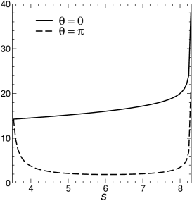
Figure 6: The $s$-dependence of $\mathcal{T}_{11}$ in forward and backward kinematics in 1+1 dimensions. Covariant calculation.

For comparison, we give in Fig. 7 the matrix elements of $\mathcal{T}_{11}$ in forward and backward scattering for the 3+1-dimensional case. The behaviour is almost the same as the 1+1-dimensional case, the main difference being the scale.

Of course, we also have in the 3+1 dimensional case the $\mathcal{T}_{23}$-element in backward scattering, but as its behaviour is very similar to the behaviour of $\mathcal{T}_{11}$, we do not show it.

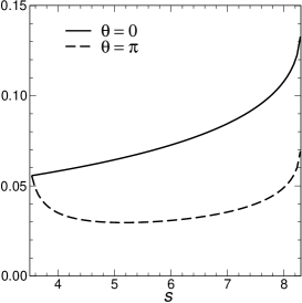
Figure 7: The $s$-dependence of $\mathcal{T}_{11}$ in forward and backward kinematics in 3+1 dimensions. Covariant calculation.

In Fig. 8, we present our results for the $s$- and $\theta$-dependence of the four form factors.

$F_{1}$                                                              $F_{2}$

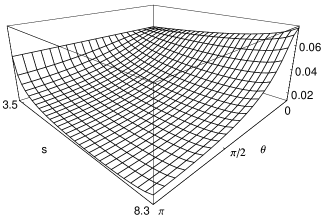
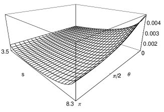
$F_{3}$                                                              $F_{4}$

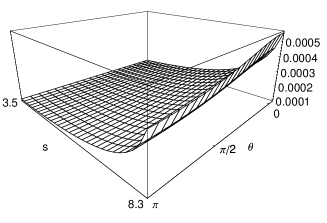
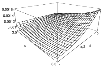
Figure 8: The $s$- and $\theta$-dependence of the form factors. Covariant calculation.

VI.2 Light-front calculation using dimensional regularization

We have calculated the $s$-dependence of the contributions of the four diagrams to $\mathcal{T}_{11}$ in 1+1 and 3+1 dimensions both in forward and in backward kinematics. The results are given in Figs. 9 - 12. Note that in these cases the contributions to the form factors cannot be calculated, as the matrix $O^{d}_{fi}$ of Sec. III.3 is singular.

In Figs. 9 and 11 the zero mode is clearly visible. In 1+1 as well as in 3+1-dimensions, diagram 1 dominates at high $s$ in forward kinematics. In backward kinematics, it is diagram 2 which contributes the most. We also see differences between 1+1 and 3+1 dimensions. The dominant diagrams are the same, but otherwise the behaviour of the amplitudes is completely different.

We should note that close to the threshold of the unitarity cut at $s=8.29$, numerical errors increase and the sum of the LF amplitudes differs from the covariant amplitude. We have checked that the covariant amplitudes agree with the LF ones to at least three decimal places for $s<5.9$ if we use 20 Gauss points for each dimension in the numerical integrals. If we increase the number of abscissas to 50, the accuracy increases to at least 5 decimal places. Thus, we conclude that the differences are purely due to numerical noise.

We have also calculated the $s$-dependences of the contributions of the four diagrams to the form factors. In Fig. 13 we show the results for a fixed angle $\theta=\pi/2$. (We do not show the results for $s>4.5$, because they show little structure.) We have summed the contributions per diagram to each form factor and compared these sums with the covariant form factors. We found that the sums and the covariant results are the same, meaning that the LF calculation is equivalent to the covariant one.

The contributions to the form factors are of the same order of magnitude as the sum at high $s$ and $\theta$. The LF form factors diverge for small $s$ and $\theta$, but their sum does not diverge since the four diagrams compensate each other, rendering the sum finite. The divergence at small $s$ and $\theta$ of the four diagrams are to some extent artefacts of the extraction procedure. However, they become important in a situation where e.g. the stretched box would be dropped. They show in a dramatic way the need to include all Fock sectors that contribute to a certain order in covariant perturbation theory.

We have obtained our results for the form factors in LFD using the extraction procedure in Sec. III.3. In this extraction procedure, we used the elements of the first row of $\mathcal{T}$ to obtain our form factors. Another choice for the four independent matrix elements of $\mathcal{T}$ gives different results for the contributions of the four diagrams. The sum, however, does not change. Furthermore, the low $s$- and $\theta$-behaviour will also not change in the sum, as this behaviour in the individual LFD contribution is just an artefact of our extraction procedure. If one would not take the four-particle intermediate-state into account, in other words neglect diagram 3, the $s$- and $\theta$-behaviour would be completely different, most dramatically at small $s$ and $\theta$.

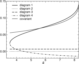
Figure 9: The $s$-dependence of the contributions of the four diagrams to $\mathcal{T}_{11}$ in forward kinematics in 1+1 dimensions. Light-front calculation.

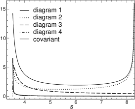
Figure 10: The $s$-dependence of the contributions of the four diagrams to $\mathcal{T}_{11}$ in backward kinematics in 1+1 dimensions. Light-front calculation.

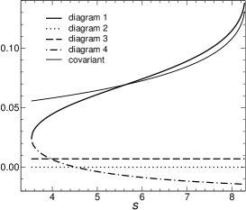
Figure 11: The $s$-dependence of the contributions of the four diagrams to $\mathcal{T}_{11}$ in forward kinematics in 3+1 dimensions. Light-front calculation using DR₂.

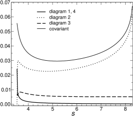
Figure 12: The $s$-dependence of the contributions of the four diagrams to $\mathcal{T}_{11}$ in backward kinematics in 3+1 dimensions. Light-front calculation using DR₂.

$F_{1}$                                                      $F_{2}$

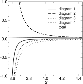
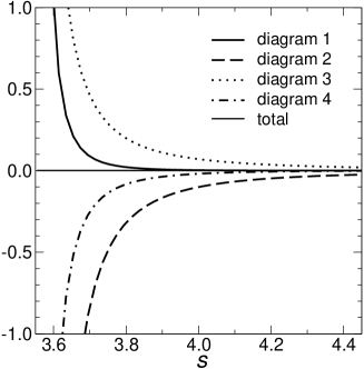
$F_{3}$                                                      $F_{4}$

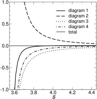
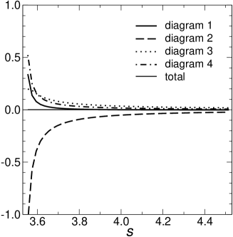
Figure 13: The $s$-dependence of the contributions of the four diagrams to the form factors for a value $\theta=\pi/2$. Light-front calculation using DR₂.

VI.3 Light-front calculation using Pauli-Villars regularization

In this subsection, we give our results of the LF calculation using Pauli-Villars regularization. In Figs. 14 and 15 we present the results in 1+1 dimensions. All the contributions of the diagrams are convergent, and so is the sum. This has to be the case, since no regularization is needed in 1+1 dimensions. Furthermore, this sum is in both cases equal to the covariant result.

The results of our calculation of the $\mathcal{T}_{11}$ matrix element in forward kinematics in 3+1 dimensions at $s=5$ are shown in Fig. 16. The logarithmic dependence is clearly visible. The divergent parts can be written in the form

$$C_{d}\ln\Lambda^{2}/\mu^{2},$$ (61)

where we use the same coefficients $C_{d}$, given by Eq. (58), as in the case of DR₂. Note, however, that this choice is not unique, as we could also subtract in addition a term of the form $C_{d}\times constant$, where $constant$ is independent of the diagram label $d$. This would not change the sum of the LF amplitudes, because the sum of the coefficients $C_{d}$ vanishes. The cancellation of the logarithmic terms is clearly visible. Finally, we note that the sum is equal to the covariant result and that neglecting the stretched box changes the results considerably, as it is needed to obtain finite results.

In Fig 17, we show the same results, but now we have subtracted the terms $C_{d}\ln\Lambda^{2}/\mu^{2}$. Again, one sees that all diagrams are now convergent so that this divergence is really the logarithmic divergence found by Van Iersel.

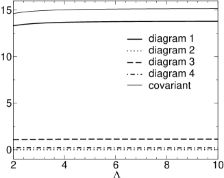
Figure 14: The $\Lambda$-dependence of the four contributions to $\mathcal{T}_{11}$ in forward kinematics in 1+1 dimensions at $s=5$. Light-front calculation with PV subtraction.

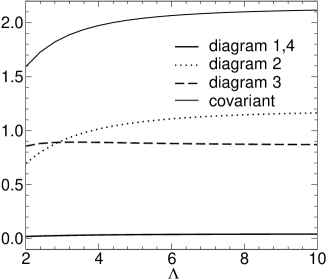
Figure 15: The $\Lambda$-dependence of the four contributions to $\mathcal{T}_{11}$ in backward kinematics in 1+1 dimensions at $s=5$. Light-front calculation with PV subtraction.

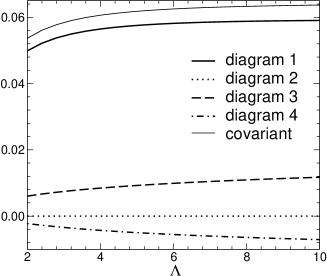
Figure 16: The $\Lambda$-dependence of the four contributions to $\mathcal{T}_{11}$ in forward kinematics in 3+1 dimensions at $s=5$. Light-front calculation with PV subtraction.

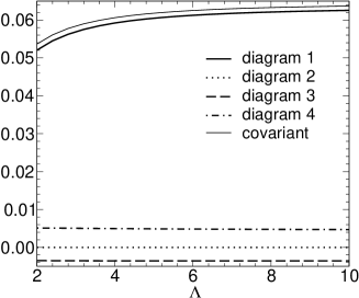
Figure 17: The $\Lambda$-dependence of the four contributions to $\mathcal{T}_{11}$ in forward kinematics in 3+1 dimensions at $s=5$. In this figure the $\ln\Lambda^{2}/\mu^{2}$-term is subtracted.

VII Conclusions

We have calculated the box diagram in generalized Yukawa theory, both in the manifestly covariant formalism and LF quantization. In the particular case we considered, this diagram can be expressed in terms of four invariant form factors.

If the calculations are carried out in $1+1$ dimensions, both approaches lead to finite integrals and the LF amplitudes add up to the covariant ones. In $3+1$ dimensions, we recovered the well-known divergences of the LF amplitudes. Using two completely different regularization methods, we succeeded to remove them and show that the finite parts of the LF amplitudes again add up to the covariant ones, while the divergent parts cancel out. There is no scheme dependence of the sum of the regularized amplitudes. One may change both regularization schemes in such a way that the individual regulated LF amplitudes in different schemes are different, but the allowed changes must not change their sum. There is no anomaly in the box diagram, opposed to the situation in the triangle diagram of the gauge theory.

A zero mode occurs, that is revealed only in special kinematical situations, because it is seen only if there is no plus-momentum transfer. In the kinematics we adopted, it shows up for special choices of the scattering angle or the energy, but one might choose the scattering plane to be perpendicular to the $z$-axis, in which case the zero mode will occur for all values of the energy and the scattering angle.

The mechanism for the occurrence of the LF singularities is easily understood. They are connected to the form of the dispersion relation for the LF energy. The appearance of the square of the transverse momentum in the numerator of the LF energy upsets the usual power counting and opens the possibility for ulraviolet divergences in LFD that are not present in the corresponding covariant calculation. From our results, one understands immediately that logarithmic divergences like the ones we have encountered in the box diagram will be present in all orders of perturbation theory.

The taming of the LF singularities can be done only by including all relevant Fock sectors. In the box diagram, it means that one may not discard the stretched box. This does not bode well for nonperturbative methods that rely on regularization, for instance of the kernel of the bound-state equation, order-by-order. It might turn out that an infinite number of counterterms is needed to regulate LF Yukawa theory.

For further study, we think that it may be useful to investigate the double box in order to learn what new singularities may occur. The double box would correspond to one more iteration of the covariant ladder kernel. From this study, we would find out whether the removal of the singularities of the box diagram is sufficient to regulate the nonperturbative calculations.

We may also try to attack this problem from a completely different angle. Namely, we may just do the nonperturbative calculation for a finite value of the Pauli-Villars mass $\Lambda$ and make a $\Lambda\to\infty$ extrapolation of the observables, e.g. the masses of the bound states. We are convinced that this program would work if the limit of $\Lambda\to\infty$ and the limit of taking an infinite number of diagrams into account commute.

Since the positivity of the LF energy and longitudinal momentum is a great advantage of the LF formulation, it would be a disappointment if none of the cures that we would like to try would work.

Appendix A Spinors

We shall use in this paper helicity spinors. The reason is that in LFD the LF boosts, which are combinations of pure boosts and rotations, form a subgroup of the Lorentz group. We get the Kogut and Soper spinors KS1970 by boosting a rest-frame spinor using a LF boost (see, e.g., Ref. BJ2002 ). We write them down explicitly for completeness. (The symbols $\pm$ refer to $s_{z}=\pm 1/2$, respectively.)

$$u_{\rm LF}({\bm{p}};+)=\frac{1}{\sqrt{4\surd 2\,p^{+}M}}\left(\begin{array}[]{c}\surd 2\,p^{+}+m\\ p^{r}\\ \surd 2\,p^{+}-m\\ p^{r}\end{array}\right),\quad u_{\rm LF}({\bm{p}};-)=\frac{1}{\sqrt{4\surd 2\,p^{+}M}}\left(\begin{array}[]{c}-p^{l}\\ \surd 2\,p^{+}+m\\ p^{l}\\ -\surd 2\,p^{+}+m\end{array}\right).$$ (62)

The matrix elements now have the structure

$$I=\left(\begin{array}[]{rl}I_{a}&I_{b}\\ -I^{*}_{b}&I^{*}_{a}\end{array}\right),\quad\Gamma^{\mu}=\left(\begin{array}[]{rl}\Gamma^{\mu}_{a}&\Gamma^{\mu}_{b}\\ -{\Gamma^{\mu}_{b}}^{*}&{\Gamma^{\mu}_{a}}^{*}\end{array}\right).$$ (63)

The explicit forms of the matrix elements are

$$I_{a} = \frac{p^{\prime\,+}+p^{+}}{2\sqrt{p^{\prime\,+}p^{+}}},\quad I_{b}=\frac{-p^{\prime\,+}p^{l}+p^{+}p^{\prime l}}{2M\sqrt{p^{\prime\,+}p^{+}}}$$

$$\Gamma^{0}_{a} = \frac{2p^{\prime+}p^{+}+{\bm{p}}^{\,\prime}_{\perp}\cdot{\bm{p}}_{\perp}+i{\bm{p}}^{\,\prime}_{\perp}\times{\bm{p}}_{\perp}+M^{2}}{2M\sqrt{2p^{\prime+}p^{+}}},\quad\Gamma^{0}_{b}=\frac{p^{\prime l}-p^{l}}{2\sqrt{p^{\prime+}p^{+}}},$$

$$\Gamma^{x}_{a} = -\frac{p^{\prime+}p^{r}+p^{+}p^{\prime l}}{2M\sqrt{p^{\prime+}p^{+}}},\quad\Gamma^{x}_{b}=-\frac{p^{\prime+}-p^{+}}{2\sqrt{p^{\prime+}p^{+}}},$$

$$\Gamma^{y}_{a} = -i\frac{p^{\prime+}p^{r}-p^{+}p^{\prime l}}{2M\sqrt{p^{\prime+}p^{+}}},\quad\Gamma^{y}_{b}=-i\frac{p^{\prime+}-p^{+}}{2\sqrt{p^{\prime+}p^{+}}},$$

$$\Gamma^{z}_{a} = \frac{2p^{\prime+}p^{+}-{\bm{p}}^{\,\prime}_{\perp}\cdot{\bm{p}}_{\perp}-i{\bm{p}}^{\,\prime}_{\perp}\times{\bm{p}}_{\perp}-M^{2}}{2M\sqrt{2p^{\prime+}p^{+}}},\quad\Gamma^{z}_{b}=-\frac{p^{\prime l}-p^{l}}{2\sqrt{p^{\prime+}p^{+}}},$$

$$\Gamma^{+}_{a} = \frac{\sqrt{p^{\prime+}p^{+}}}{M},\quad\Gamma^{+}_{b}=0,$$

$$\Gamma^{-}_{a} = \frac{{\bm{p}}^{\,\prime}_{\perp}\cdot{\bm{p}}_{\perp}+i{\bm{p}}^{\,\prime}_{\perp}\times{\bm{p}}_{\perp}+M^{2}}{2M\sqrt{p^{\prime+}p^{+}}},\quad\Gamma^{-}_{b}=\frac{p^{\prime l}-p^{l}}{2\sqrt{p^{\prime+}p^{+}}}.$$ (64)

In the kinematics we adopt, we find explicitly for particle $1$

$$I_{a}(1) = \frac{2E+p(1+\cos\theta)}{2\sqrt{(E+p)(E+p\cos\theta)}},\quad I_{b}(1)=\frac{(E+p)p\sin\theta}{2M\sqrt{(E+p)(E+p\cos\theta)}};$$

$$\Gamma^{0}_{a}(1) = \frac{(E+p)(E+p\cos\theta)+m^{2}}{2M\sqrt{(E+p)(E+p\cos\theta)}},\quad\Gamma^{0}_{b}(1)=\frac{p\sin\theta}{2\sqrt{(E+p)(E+p\cos\theta)}};$$

$$\Gamma^{x}_{a}(1) = \frac{(E+p)p\sin\theta}{2M\sqrt{(E+p)(E+p\cos\theta)}},\quad\Gamma^{x}_{b}(1)=-\frac{p(1-\cos\theta)}{2\sqrt{(E+p)(E+p\cos\theta)}};$$

$$\Gamma^{y}_{a}(1) = i\frac{(E+p)p\sin\theta}{2M\sqrt{(E+p)(E+p\cos\theta)}},\quad\Gamma^{y}_{b}(1)=i\frac{p(1-\cos\theta)}{2\sqrt{(E+p)(E+p\cos\theta)}};$$

$$\Gamma^{z}_{a}(1) = \frac{(E+p)(E+p\cos\theta)-M^{2}}{2M\sqrt{(E+p)(E+p\cos\theta)}},\quad\Gamma^{z}_{b}(1)=-\frac{p\sin\theta}{2\sqrt{(E+p)(E+p\cos\theta)}}.$$ (65)

For particle $2$ the matrix elements are found by substituting $-p$ for $p$ in the expressions for particle $1$.

A simple check on these expressions is to go to the forward limit, $\theta=0$, where the matrix elements of the identity must reduce to $\delta_{\lambda^{\prime}\lambda}$ and of the $\gamma$-matrices to $p^{\mu}\,\delta_{\lambda^{\prime}\lambda}/m$.

Appendix B Integrals needed in dimensional regularization

We need explicit expressions for the integrals over $\vec{k}^{\perp}$ since some of the integrals are divergent. In this appendix, we show how to regularize these divergences using DR₂.

In LFD, regularization is needed in the transverse directions only. In dimensional regularization, we calculate the integrals as an analytic function of the dimensionality of these directions. We change the number of dimensions from 2 to D. The integrals are changed according to

$$\int\!\frac{\mathrm{d}^{2}k^{\perp}}{(2\pi)^{2}}\frac{\left(\vec{k}^{\perp}\right)^{2r}}{\left(\left(\vec{k}^{\perp}\right)^{2}+C^{2}\right)^{s}}\to\mu^{2-D}_{s}\int\!\frac{\mathrm{d}^{D}k^{\perp}}{(2\pi)^{2}}\frac{\left(\vec{k}^{\perp}\right)^{2r}}{\left(\left(\vec{k}^{\perp}\right)^{2}+C^{2}\right)^{s}}=\bar{I}^{r}_{s}.$$ (66)

Now, we take $D=2-2\epsilon$ to obtain

$$\bar{I}^{r}_{s}=\mu^{2\epsilon}_{s}\frac{1}{(4\pi)^{D/2}}\frac{\Gamma(r+D/2)\Gamma(s-r-D/2)}{\Gamma(D/2)\Gamma(s)}\left(\frac{1}{C^{2}}\right)^{s-r-D/2}.$$ (67)

For the divergent integral $\bar{I}^{2}_{3}$, we find

$$\bar{I}^{2}_{3}=\frac{1}{4\pi}\left[\frac{1}{\epsilon}-\gamma-\frac{3}{2}+\ln\left(\frac{4\pi\mu^{2}_{s}}{C^{2}}\right)\right].$$ (68)

The other integrals we need are completely regular;

$$\bar{I}^{0}_{3} = \frac{1}{8\pi}\frac{1}{C^{4}},$$

$$\bar{I}^{1}_{3} = \frac{1}{8\pi}\frac{1}{C^{2}}.$$ (69)

References

- (1) P.A.M. Dirac, Rev. Mod. Phys. 21, 392 (1949).
- (2) S.J. Brodsky, H.-C. Pauli, and S. Pinsky, Phys. Rep. 301, 299 (1998).
- (3) C.-R. Ji and C. Mitchell, Phys. Rev. D 64, 085013 (2001).
- (4) C.-R. Ji, G.-H. Kim, and D.-P. Min, Phys. Rev. D 64, 025009 (2001); Phys. Rev. D 58, 105020 (1998).
- (5) S.J. Brodsky, C.-R. Ji, and M. Sawicki, Phys. Rev. D 32, 1530 (1985).
- (6) J.H.O. Sales, T. Frederico, B.V. Carlson, and P.U. Sauer, Phys. Rev. C 61, 044003 (2000).
- (7) J.H.O. Sales, T. Frederico, B.V. Carlson, and P.U. Sauer, Phys. Rev. C 63, 064003 (2001).
- (8) R.J. Perry, A. Harindranath, and K.G. Wilson, Phys. Rev. Lett. 65, 2959 (1990).
- (9) S. Głazek, A. Harindranath, S. Pinsky, J. Shigemitsu, and K.G. Wilson, Phys. Rev. D 47, 1599 (1993).
- (10) B.L.G. Bakker, M.A. DeWitt, C.-R. Ji, and Y. Mishchenko, Phys. Rev. D 72, 076005 (2005).
- (11) B.L.G. Bakker and C.-R. Ji, Phys. Rev. D 71, 053005 (2005).
- (12) M. van Iersel, Few-Body Systems 36, 133 (2005).
- (13) R. Karplus, C.M. Sommerfield, and E.H. Wichmann, Phys. Rev. 114, 376 (1959)
- (14) R.J. Eden, P.V. Landshoff, D.I. Olive, and J.C. Polkinghorne, The analytic S-matrix, (Cambridge UP, Cambridge, 1966)
- (15) J.B. Kogut and D.E. Soper, Phys. Rev. D 1, 2901 (1970).
- (16) B.L.G. Bakker and C.-R. Ji, Phys. Rev. D 65, 073002 (2002).
- (17) E. Leader, Spin in Particle Physics, (Cambridge University Press, Cambridge, 2001).
- (18) K. Erkelenz, Phys. Rept. 13, 191 (1974).
- (19) N.E. Ligterink and B.L.G. Bakker, Phys. Rev. D 52, 5954 (1995).
- (20) S.J. Brodsky, J.R. Hiller, and G. McCartor, Ann. Phys. 321, 1240 (2006)
- (21) M. van Iersel, Aspects of Bound-State Calculations in Light-Front Dynamics, PhD-thesis, Vrije Universiteit, Amsterdam (2004)