We discuss Wu-Yang type solutions of Maxwell-Chern-Simons and Yang-Mills-Chern-Simons theories. There exists a natural scale of length which is determined by the inverse topological mass $\nu\sim ng^{2}$. We obtain the non-abelian solution by means of a $SU(2)$ gauge transformation of Dirac magnetic monopole type solution. In the abelian case, field strength locally determines the gauge potential up to a closed term via self-duality equation. We introduce a transformation of the gauge potential using dual field strength which can be identified with the gauge transformation in the abelian solution. Then we present Hopf map $S^{3}\longrightarrow S^{2}$ including the topological mass. This leads to a reduction of the field equation onto $S^{2}$ using local sections of $S^{3}$. The local solutions possess a composite structure consisting of both magnetic and electric charges. These naturally lead to topologically massive Wu-Yang solution which is based on patching up the local potentials by means of a gauge transformation. We also discuss solutions with different first Chern numbers. There exist a fundamental scale $\lambda=2\pi/g^{2}$ over which the gauge function is single-valued and periodic for any integer $n$ in addition to the fact that it has a smaller period $\lambda/n$. We also discuss Dirac quantization condition. We present a stereographic view of the fibres in the Hopf map. Meanwhile Archimedes map yields a simple geometric picture for the Wu-Yang solution. We also discuss holonomy of the gauge potential and the dual-field on $S^{2}$. Finally we point out a naive identification of the natural length scale introduced by the topological mass with Hall resistivity.

1 Introduction

Topologically massive gravity and gauge theory are dynamical theories which are specific to three dimensions [1, 2], [3]. They are qualitatively different from the Einstein gravity and the Yang-Mills gauge theory beside their mathematical elegance and consistency.

The most distinctive feature of the topologically massive gauge theories is the existence of a natural scale of length introduced by the topological mass: $[\nu]=[g]^{2}=L^{-1}$ [4], [5], in geometric units ($h=1$, $c=1$). The Dirac monopole [6] type solution of the Maxwell-Chern-Simons electrodynamics in a space with euclidean signature is an example of the essential new feature introduced by the topological mass [7]. This is a physical system which is a priori unrelated to gravity but which nevertheless requires curved space for its existence [7].

We discuss euclidean topologically massive Wu-Yang type solutions [8, 9], [10] of the Maxwell-Chern-Simons (MCS) and the Yang-Mills-Chern-Simons (YMCS) theories on de Sitter (dS) space $S^{3}$.

In section 2 we present, after a brief account of the YMCS theory, the geometric frame including the natural scale of length which is determined by the topological mass. We use an intrinsic arclength parameterization. This endows us with a dimensionally consistent framework for our solutions in geometrical terms. We obtain the non-abelian solution by embedding the Dirac solution [7] into the YMCS theory by means of a $SU(2)$ gauge transformation [8, 9], [10].

We return to the MCS theory in section 3. In the topologically massive electrodynamics, field strength locally determines the gauge potential up to a closed term via self-duality equation [11], [12], [13]. We introduce a transformation of the gauge potential using the dual-field strength. This will lead to the gauge function in Wu-Yang solution in terms of electric charge.

Then we present Hopf map $S^{3}\longrightarrow S^{2}$ including the topological mass [14, 15, 16]. This leads to a reduction of the field equation onto $S^{2}$ using local sections of $S^{3}$. The Hopf map yields local gauge potentials on $S^{2}$ which differ by a gauge transformation. This gives rise to topologically massive Wu-Yang solution. The gauge functions, in both the abelian and non-abelian cases, contain the topological mass $\nu\sim ng^{2}$ which yields the strength $\nu/g\sim ng$ for potentials. This is analogous to the non-massive Wu-Yang monopole which consist of the dimensionless factor $eg$.

The local solutions have a composite structure consisting of both magnetic and electric charges which are related via integral of the field equation. The gauge function can equivalently be given in terms of either the magnetic charge or the electric charge. Conversely the integrated field equation naturally gives rise to Wu-Yang type solutions on $S^{2}$ [8, 9], [10] and to loop-variables [17, 18]. We also consider solutions with different First Chern numbers.

In section 4, we present three geometric structures which arise in connection with our solutions. We briefly present a stereographic view of the fibres in the Hopf map [19], [20, 21]. Meanwhile Archimedes map [22], [23] provides a simple geometric picture for the Wu-Yang solution on $S^{2}$. We also express geometric phase [24], [25], [26, 27] suffered by a vector upon parallel transport on $S^{2}$ [23], [28] in terms of holonomy of the gauge potential or the dual-field [29, 30, 31, 32], [33], [34].

Then we discuss quantization of the topological mass: $\nu=ng^{2}$ and the length scale determined by it in section 5. There exist a fundamental scale $\lambda=2\pi/g^{2}$ over which the gauge function is single-valued and periodic for any integer $n$ in addition to the fact that it has a smaller period $\lambda/n$. We discuss the First Chern number and the quantization of the topological mass in terms of winding numbers of maps of circles. We also discuss Dirac quantization condition.

The geometric framework presented here might provide a naive explanation for the integer quantum Hall effect if the Hall resistance could be identified with the natural scale of length introduced by the topological mass.

The literature consists of various discussions on quantization of the topological mass and topological aspects of Wu-Yang type constructions (with no solution) [35, 36, 37, 38], beside different monopole/instanton type solutions [39, 40], [41, 42]. However there arise conflicting arguments, see for example [36, 37], because the essential new feature introduced by the topological mass is ignored in topological discussions, except a few remarks [41, 42]. To the knowledge of the author, the solutions and geometric constructions presented here which clarify this issue are lacking in the literature .

A lorentzian version of these solutions and structures on AdS space was given by the same author [43]. The connection of the MCS theory with contact geometry and curl transformation was discussed in [44].

2 The Non-Abelian Gauge Theory

2.1 Yang-Mills-Chern-Simons Theory

The topologically massive $SU(2)$ YMCS theory is given by the dimensionless action

$$S_{YMCS} = S_{YM}+S_{CS}$$

$$= -\frac{1}{2}\left[\int tr\bigg{(}F\wedge*F\bigg{)}-\nu\int tr\left(F\wedge A+\frac{1}{3}gA\wedge A\wedge A\right)\right],$$

where $\nu$ is the topological mass. We include the factor containing the gauge coupling constant $g$ in (2.1) in expressions for the field and the gauge potential because of underlying geometric reasons that will become clear in advance. This will lead to strength $g$ for the potential upon assuming quantization of the topological mass. The YMCS action (2.1) yields the field equation

$$D*F-\nu F=0,$$ (2)

where $D$ is the gauge covariant exterior derivative. The field $2$-form also satisfies the Bianchi identity

$$DF=0.$$ (3)

The covariant exterior derivative $D$ respectively acts as $D*F=\left(d-g\{A,\,\,\}\right)*F$ and $DF=\left(d-g[A,\,\,]\right)F$ on the dual field $1$-form $*F$ and the field $2$-form $F$. Here $\{\,\,,\,\,\}$ denotes the anti-commutator and $[\,\,,\,\,]$ the commutator.

Action (2.1) is not invariant under non-abelian large gauge transformations

$$A^{\prime}=U^{-1}AU-\frac{1}{g}U^{-1}dU.$$ (4)

It changes by

$$W=-8\pi^{2}\frac{\nu}{g^{2}}\,w,$$ (5)

neglecting a surface term that vanishes under suitable asymptotic convergence conditions on $U$ [1, 2], [3]. Here $w$ is the integer winding number

$$w=\frac{1}{48\pi^{2}}\int tr\left(U^{-1}dU\wedge U^{-1}dU\wedge U^{-1}dU\right),$$ (6)

of the gauge transformation [1, 2], [3]. Therefore the large gauge transformations, which are labeled by the winding number $w$, have a non-trivial contribution to the action.

In the lorentzian case if we demand the expression $\exp(iS)$ to be gauge invariant in order to have a well-defined quantum theory via path-integrals, then the change (5) can be tolerated if the topological mass is quantized as

$$\nu=\frac{1}{4\pi}ng^{2},$$ (7)

[1, 2], [3].

We remark that the action, the field equation and the solutions presented here, which are defined on a curved space with euclidean signature, are all real valued. We shall refer the relation: $\nu\sim ng^{2}$ as the quantization of the topological mass no matter if $n$ is an integer until section 5. Because this relation will naturally arise in our solutions.

2.2 The Natural Scale of Length

We shall consider the MCS and YMCS theory over a space with the co-frame consisting of the modified left-invariant basis $1$-forms of Bianchi type $IX$ in Euler parameters [7]. The topological mass introduces a geometric scale of length. We shall use an intrinsic arclength parameterization where the arclength parameters are independent of the length scale introduced by the topological mass.

We scale the unmodified co-frame with the dimensionful factor $1/\nu$. This yields

$$\omega^{1} = -\sin(\nu\psi)d\theta+\cos(\nu\psi)\sin(\nu\theta)d\phi$$

$$\omega^{2} = \cos(\nu\psi)d\theta+\sin(\nu\psi)\sin(\nu\theta)d\phi$$ (8)

$$\omega^{3} = d\psi+\cos(\nu\theta)d\phi,$$

in terms of the intrinsic (half) arclength coordinates

$$\theta=\frac{1}{2}R\tilde{\theta}\hskip 14.22636pt,\hskip 14.22636pt\phi=\frac{1}{2}R\tilde{\phi}\hskip 14.22636pt,\hskip 14.22636pt\psi=\frac{1}{2}R\tilde{\psi}$$ (9)

$$\hskip 8.53581pt=\frac{1}{\nu}\tilde{\theta}\hskip 48.36967pt=\frac{1}{\nu}\tilde{\phi}\hskip 48.36967pt=\frac{1}{\nu}\tilde{\psi},$$

which have the dimension of length: $[\theta]=[\phi]=[\psi]=L$. This amounts to scaling the Cartan-Killing metric by the factor $1/\nu^{2}$

$$ds^{2}=\eta_{ab}\omega^{a}\omega^{b}\hskip 28.45274pt\eta_{ab}=diag(1,1,1)$$ (10)

$$\hskip 19.91692pt=d\theta^{2}+d\phi^{2}+2\cos(\nu\theta)d\phi d\psi+d\psi^{2}$$

$$\hskip 19.91692pt=d\theta^{2}+\sin^{2}\left(\nu\theta\right)d\phi^{2}+[d\psi+\cos(\nu\theta)d\phi]^{2},$$

which yields the de Sitter space $S^{3}$. The radius of the $3$-sphere is scaled by the same factor: $R=(1/\nu)\tilde{R}=(1/\nu)2$. The parameters $\theta$, $\phi$, $\psi$ respectively represent the half-length of arcs which corrrespond to the Eulerian angles $\tilde{\theta}=\nu\theta$, $\tilde{\phi}=\nu\phi$, $\tilde{\psi}=\nu\psi$ on the $3$-sphere of radius $R=2/\nu$. Thus (10) is the metric on the $3$-sphere $S^{3}$ of radius $R=2/\nu$ which is parameterized in terms of the (half) Eulerian arclengths. The co-frame (2.2) determines a unique orientation on this sphere. The scalar curvature $\mathcal{R}$ of this $3$-sphere is determined by its radius $R$

$${\mathcal{R}}=\frac{6}{R^{2}}=\frac{3}{2}\,\,\nu^{2},$$ (11)

[45]. Note that the arclength parameters are independent of the length scale determined by the inverse topological mass. We shall only consider rotational degrees of freedom which are associated with the intrinsic arclengths.

This $3$-sphere $S^{3}$ can be embedded into the euclidean space $\mathbf{R^{4}}$

$$(y^{1})^{2}+(y^{2})^{2}+(y^{3})^{2}+(y^{4})^{2}=R^{2}\hskip 8.53581pt,\hskip 8.53581ptR=\frac{2}{\nu},$$ (12)

[7] by the correspondence

$$y^{1}=R\cos\left(\nu\frac{\theta}{2}\right)\cos\left(\nu\frac{\psi+\phi}{2}\right)\hskip 8.53581pt,\hskip 8.53581pty^{2}=R\cos\left(\nu\frac{\theta}{2}\right)\sin\left(\nu\frac{\psi+\phi}{2}\right)$$

(13)

$$y^{3}=R\sin\left(\nu\frac{\theta}{2}\right)\cos\left(\nu\frac{\psi-\phi}{2}\right)\hskip 8.53581pt,\hskip 8.53581pty^{4}=R\sin\left(\nu\frac{\theta}{2}\right)\sin\left(\nu\frac{\psi-\phi}{2}\right),$$

where $R=2/\nu$. The flat metric

$$ds^{2}=(dy^{1})^{2}+(dy^{2})^{2}+(dy^{3})^{2}+(dy^{4})^{2},$$ (14)

on $\mathbf{R^{4}}$ reduces to (10) with this correspondence.

The Hodge-duality relations and the Maurer-Cartan equations for the basis (2.2) immediately lead to the result that the MCS field equation: $d(*F-\nu A)=0$ will be identically satisfied for the gauge potential $1$-form: $A=-(\nu/g)\omega^{3}$ [7]. The field equation is given by the derivative of the self-duality condition: $*F-\nu A=0$ for the topologically massive abelian gauge fields [11], [12]. The MCS action vanishes for this potential: $S_{MCS}[A]=0$. Note that a change in the orientation leads to a change of sign in the field equation.

We shall define the Hopf map $S^{3}\longrightarrow S^{2}$ including the topological mass in section 3.2. We also scale the radius of the unit $2$-sphere by the same factor $1/\nu$

$$(x^{1})^{2}+(x^{2})^{2}+(x^{3})^{2}=r^{2}\hskip 8.53581pt,\hskip 8.53581ptr=\frac{1}{\nu}.$$ (15)

The correspondence with the metric on $S^{2}$ is given by

$$x^{1}=r\sin(\nu\theta)\cos(\nu\phi)\hskip 8.53581pt,\hskip 8.53581ptx^{2}=r\sin(\nu\theta)\sin(\nu\phi)\hskip 8.53581pt,\hskip 8.53581ptx^{3}=r\cos(\nu\theta),$$ (16)

where $r=1/\nu$. This provides an embedding of this $2$-sphere $S^{2}$ into the space $\mathbf{R^{3}}$ with radius $r=1/\nu$. The flat metric

$$ds^{2}=(dx^{1})^{2}+(dx^{2})^{2}+(dx^{3})^{2},$$ (17)

on $\mathbf{R^{3}}$ reduces to the metric

$$ds^{2}=d\theta^{2}+\sin^{2}\left(\nu\theta\right)d\phi^{2},$$ (18)

on $S^{2}$ with this correspondence. Thus (18) is the metric on the $2$-sphere $S^{2}$ of radius $r=1/\nu$ which is parameterized in terms of the length of spherical arcs corresponding to the spherical angles $\tilde{\theta}=\nu\theta$, $\tilde{\phi}=\nu\phi$. More precisely, $\theta$ is the length of the geodesic arc from the north pole to the south and $\phi$ is the length of the geodesic arc on the equator.

The range of the parameters $\theta$, $\phi$, $\psi$ are determined by the topological mass. The arclength $\phi$ on the equator of $S^{2}$ uniquely defines the angle $\tilde{\phi}=\nu\phi$ for any parallel. The length of an arc, on the parallel determined by $\theta=(1/\nu)\tilde{\theta}$, which corresponds to the angle $\tilde{\phi}$ is

$$\frac{\sin(\nu\theta)}{\nu}\tilde{\phi}=\sin(\nu\theta)\phi.$$ (19)

This reduces to the arclength on the equator: $\phi=(1/\nu)\tilde{\phi}$ when $\tilde{\theta}=\nu\theta=\pi/2$. The coordinate $\phi$ which is well-defined for any point except the poles on $S^{2}$ changes from $\phi=0$ to $\phi=2\pi/\nu$ round about any parallel.

2.3 The Topologically Massive Non-abelian Solution

First consider the solution which is given by the gauge potential $1$-form:

$$A=-\frac{\nu}{g}\,\omega^{3}\,\tau_{3}=-\frac{\nu}{g}\,\Big{[}d\psi+\cos(\nu\theta)d\phi\Big{]}\tau_{3},$$ (20)

[7]. Here $\tau_{i}=\sigma_{i}/2i$ where $\sigma_{i}$ are the Pauli spin matrices. The factor $\nu/g$ yields $(1/4\pi)ng$ for the strength of the potential $A$ upon quantization of the topological mass (7). This is analogous to Dirac’s quantization condition $eg=n$ which leads to strength $g$ for the non-abelian solution upon a gauge transformation of the Dirac’s monopole potential [9], [10].

A gauge transformation of the potential (20) necessarily contains the topological mass inherently in the gauge function, because it also appears in the potential (20). This is intuitively analogous to the gauge transformation in the non-massive Wu-Yang monopole that contains the dimensionless factor $eg$. In our case this is basically due to the arclength parameterization. The gauge function which embeds the topologically massive abelian solution (20) into the YMCS theory is an element of the group $SU(2)$ [46], [47]. This is given by normalizing the radius $R$ of $S^{3}$ which is parameterized with the Eulerian arclengths as

$$\hskip 22.76219ptU=\frac{1}{R}\left(\begin{array}[]{cc}z^{1}&z^{2}\\ -\bar{z}^{2}&\bar{z}^{1}\end{array}\right)=\exp{(-\nu\gamma\tau_{3})}\exp{(-\nu\beta\tau_{2})}\exp{(-\nu\alpha\tau_{3})}.$$ (23)

Here $z^{1}=y^{1}+iy^{2}$, $z^{2}=y^{3}+iy^{4}$. We identify the Euler parameters as $\alpha=\phi,\,\,\beta=\theta,\,\,\gamma=\psi$. This is the analog of the gauge transformation which embeds the Dirac monopole solution into the $SU(2)$ YM theory [9], [10]. Note that $U\rightarrow 1$ as $\nu\rightarrow 0$.

The gauge transformation (4) with the gauge function (23) have winding number $w=1$ (6). It yields the potential $1$-form

$$A^{\prime}=U^{-1}AU-\frac{1}{g}U^{-1}dU$$ (24)

$$\hskip 17.07164pt=-\frac{\nu}{g}\,\bigg{\{}\Big{[}\sin(\nu\phi)\tau_{1}-\cos(\nu\phi)\tau_{2}\Big{]}d\theta$$

$$\hskip 28.45274pt+\Big{[}\cos(\nu\theta)\cos(\nu\phi)\tau_{1}+\cos(\nu\theta)\sin(\nu\phi)\tau_{2}-\sin(\nu\theta)\tau_{3}\Big{]}\sin(\nu\theta)d\phi\bigg{\}}.$$

This gives rise to the field $2$-form

$$F^{\prime}=dA^{\prime}-gA^{\prime}\wedge A^{\prime}=U^{-1}FU$$ (25)

$$\hskip 17.07164pt=\frac{\nu^{2}}{g}\Big{[}\sin(\nu\theta)\cos(\nu\phi)\tau_{1}+\sin(\nu\theta)\sin(\nu\phi)\tau_{2}+\cos(\nu\theta)\tau_{3}\Big{]}$$

$$\hskip 236.15787pt\sin(\nu\theta)d\theta\wedge d\phi.$$

The dual field $1$-form covariantly transforms as: $*F^{\prime}=U^{-1}*FU$. The field equation (2) and the Bianchi identity (3) are identically satisfied since they also covariantly transform. This is the topologically massive non-abelian Wu-Yang solution which is the generalization of the non-massive Wu-Yang solution given in [9].

We have three observations which are based on dimensional arguments in the equations (20), (23), (24), (25).

(i) The gauge function necessarily contains the topological mass as in (23).
(ii) The strength $\nu/g$ of the abelian gauge potential (20) is crucial for finding
       the field $2$-form (25) in the non-abelian case. One finds the correct ex      pression for the field $2$-form with this choice.
(iii) This is associated with the quantization of the topological mass.

Thus if the strength of the potential is given by $\nu/g$ then we inevitably arrive at condition (7), because this yields $\nu/g=(1/4\pi)ng$ as the strength of the potential. Conversely, if one starts with a potential with strength $(1/4\pi)ng$, then one needs to use (7) in finding the non-abelian gauge potential $A^{\prime}$ (24) and field $F^{\prime}$ (25). Moreover the YMCS field equation reduces to condition (7) which will be identically satisfied. Note that in this discussion, number $n$ is a free parameter. The gauge coupling strength and the electric charge are denoted with $g$. The factor of $1/4\pi$ in the topological mass (7) is included in the strength of the potential for the sake of conciseness.

Action (2.1) for the potential (24) reduces to the Yang-Mills term because the Chern-Simons piece vanishes

$$S_{YMCS}[A^{\prime}]=-8\pi^{2}\frac{\nu}{g^{2}}=-2\pi n.$$ (26)

This is equal to change $W$ (5) in the action due to the gauge transformation (23) which have winding number $w=1$. The other term which arise in the action as a result of the gauge transformation (23) vanishes. The quantization of the topological mass also leads to

$${\mathcal{R}}\sim n^{2}g^{4},$$ (27)

for the scalar curvature (11).

3 The Abelian Gauge Theory

3.1 Maxwell-Chern-Simons Theory

The action for MCS theory is

$$S_{MCS} = S_{M}+S_{CS}$$

$$= -\frac{1}{2}\,\,\frac{1}{2\pi}\,\left(\int F\wedge*F-\nu\int F\wedge A\right).$$

For later convenience, we explicitely write $1/2\pi$ in (7) as an overall factor in the action. We also adopt a slight change of convention in the abelian potential: $A=-(1/2)(\nu/g)\omega^{3}$ and the topological mass is now given as: $\nu=ng^{2}$. The MCS action (3.1) yields the field equation

$$\left(*d-\nu\right)*F=0.$$ (29)

The field $2$-form also satisfies the Bianchi identity $dF=0$. We can easily derive

$$(\triangle-\nu^{2})F=0\hskip 14.22636pt,\hskip 14.22636pt(\triangle-\nu^{2})*F=*(\triangle-\nu^{2})F=0,$$ (30)

where $\triangle=(d+\delta)^{2}$ is the Laplace-Beltrami operator. The operator $\triangle-\nu^{2}$ is factorizable as

$$\triangle-\nu^{2}=(d*-\nu)(d*+\nu)=(d*+\nu)(d*-\nu).$$ (31)

We find

$$\left(*d-\nu\right)A=\nu\alpha,$$ (32)

if we integrate (29), after taking the Hodge-dual. Here $\alpha$ is a closed $1$-form: $d\alpha=0$ which can be made to vanish by means of a gauge transformation if locally $\alpha=dB$. Thus the topologically massive field locally determines the potential up to a gauge term via the self-duality equation

$$\left(*d-\nu\right)A^{\prime}=0,\hskip 14.22636pt\hskip 14.22636ptF^{\prime}=F=dA^{\prime},$$ (33)

where $A^{\prime}=A+\alpha$ [11], [12]. Therefore the field equation is identically satisfied for a self-dual field/potential $A^{\prime}$. Because the equations (29) and (33) are symmetric under the interchange $*F\leftrightarrow\nu A$. Hence we can also treat the dual-field $1$-form $*F$ as a gauge potential in the field equation (29). As a result the field equation (29) reduces to finding the strength of the potential which is determined by the field strength itself

$$F^{\prime}=dA^{\prime}=\frac{1}{\nu}d*F=F.$$ (34)

The Bianchi identity $dF^{\prime}=0$ is also satisfied. The Maxwell and the Chern-Simons terms in the MCS action (3.1) interchange under this symmetry as $F^{\prime}=F$ is kept fixed.

We can define yet another potential $\tilde{A}$ by the transformation

$$\tilde{A}=\frac{1}{\nu}\,\left(*d+\nu\right)A=A+\frac{1}{\nu}*F,$$ (35)

which is motivated by this interchange symmety. The right-hand side in (35) is the self-duality equation with an opposite sign for the topological mass. The new potential $\tilde{A}$ transforms as a connection under the abelian gauge transformations. The potential $\tilde{A}$ and the field

$$\tilde{F}=d\tilde{A}=\frac{1}{\nu}\left(d*+\nu\right)F,$$ (36)

respectively satisfy the equations (32) and (29) by virtue of (30), (31). The field $\tilde{F}$ also satisfies the Bianchi identity $d\tilde{F}=0$. The equations (29) and (32) in turn yield $\tilde{A}=2A+\alpha$ and $\tilde{F}=2F$. A variant of this transformation (35) is also observed in [48] and similar features are used in [49, 50]. In fact, with a similar reasoning, one can introduce higher order terms of type $(\frac{1}{\nu}*d)^{i}A$ where $i=1,2,3,...$. The topologically massive gauge theory is related to the CS theory through such an expansion of field redefinition in [51], [52, 53].

The equation (36) leads to the trivial conclusion that the field $2$-form $F$ which satisfies the field equation (29) becomes a source for the field equation with an opposite sign for the topological mass

$$\left(*d+\nu\right)*F=J.$$ (37)

Here the source $1$-form is given as $J=2\nu*F$. In this case: $d*J=0$ since $dF=0$. The self-duality $*F=\nu A$ yields: $J=2\nu^{2}A=2\triangle A$ (30).

We shall see in section 3.4 that we can interpret (35) as a gauge transformation

$$A^{\prime}=A-\frac{i}{g}U^{-1}dU,$$ (38)

of the potential $A$ on the $2$-sphere. We find that the gauge function is

$$U=\exp\left(i\frac{g}{\nu}\oint*F\right)=\exp\left[ig\oint(A+\alpha)\right],$$ (39)

upon the identification

$$\frac{1}{\nu}\,*F=-\frac{i}{g}d\ln U,$$ (40)

and using the self-duality equation (33). This is the gauge function which will arise in the topologically massive Wu-Yang solution in terms of a loop integral that yields the electric charge.

3.2 The Hopf Map with the Topological Mass

In this section we present the Hopf map $S^{3}\longrightarrow S^{2}$ including the topological mass. This leads to local topologically massive Wu-Yang potentials on $S^{2}$ upon using specific sections of $S^{3}$ which is locally given as a $S^{1}$ bundle over $S^{2}$: $S^{3}\approx S^{1}\times S^{2}$ [14, 15, 16]. The difference from the non-massive Wu-Yang monopole [9], [10] which is essentially described by a $U(1)$ principal bundle over the unit $2$-sphere is the introduction of a natural scale of length by the topological mass. We refer the reader to [19, 20, 21, 54, 55, 56, 57, 58, 59] for the basic concepts of the Hopf map and its relation to Dirac monopole [14, 15, 16] which we adapt here with the inclusion of the topological mass. For a discussion of Wu-Yang type multi-monopole solutions see [60].

The Hopf map $S^{3}\longrightarrow S^{2}$ is given as

$$x^{1}=2\frac{r}{R^{2}}\left(y^{1}y^{3}+y^{2}y^{4}\right),$$

$$x^{2}=2\frac{r}{R^{2}}\left(y^{2}y^{3}-y^{1}y^{4}\right),$$ (41)

$$x^{3}=\frac{r}{R^{2}}\left[(y^{1})^{2}+(y^{2})^{2}-(y^{3})^{2}-(y^{4})^{2}\right],$$

[14], [15, 16]. The sections of the $3$-sphere (2.2) corresponding to $\phi=-\psi$ and $\phi=\psi$ are respectively

$$z^{1}=R\cos\left(\frac{\nu\theta}{2}\right)=R\frac{r}{\sqrt{r^{2}+|w|^{2}}},$$ (42)

$$z^{2}=R\sin\left(\frac{\nu\theta}{2}\right)\exp(-i\nu\phi)=R\frac{w}{\sqrt{r^{2}+|w|^{2}}},$$

$$\hskip 28.45274ptw=r\frac{x^{1}-ix^{2}}{r+x^{3}}=r\frac{z^{2}}{z^{1}}=r\tan\left(\frac{\nu\theta}{2}\right)\exp(-i\nu\phi),$$

and

$$z^{1}=R\cos\left(\frac{\nu\theta}{2}\right)\exp(i\nu\phi)=R\frac{z}{\sqrt{r^{2}+|z|^{2}}},$$

$$z^{2}=R\sin\left(\frac{\nu\theta}{2}\right)=R\frac{r}{\sqrt{r^{2}+|z|^{2}}},$$ (43)

$$\hskip 28.45274ptz=r\frac{x^{1}+ix^{2}}{r-x^{3}}=r\frac{z^{1}}{z^{2}}=r\cot\left(\frac{\nu\theta}{2}\right)\exp(i\nu\phi).$$

Here $z$ and $w$ are respectively the stereographic projection coordinates of the southern hemi-sphere $U_{S}$ and the northern hemi-sphere $U_{N}$ of $S^{2}$ projected from the north pole and the south pole to the equatorial plane. They satisfy $zw=r^{2}$ (42), (3.2).

The inverse image of a point in $S^{2}$ is given by either: $z^{1}=\frac{1}{r}zz^{2}$ or $z^{2}=\frac{1}{r}wz^{1}$ where $|z^{1}|^{2}+|z^{2}|^{2}=R^{2}$. These are the intersections of $S^{3}$ with hyperplanes passing through the origin. Thus for every point in $S^{2}$, there exists a $S^{1}$ fibre which is a great circle of radius $R=2/\nu$ in $S^{3}$ [21, 54, 55, 56]. These are parameterized as $\exp(-\nu\psi\tau_{3})$ or simply $\exp(i\nu\psi/2)$ [54]. We shall present a stereographic view of these fibres in section 4.

The $3$-sphere $S^{3}$ is locally given as $S^{1}\times S^{2}$. However $S^{1}\times S^{2}$ is globally distinct [15]. Because on $S^{2}$ the angular coordinate $\tilde{\phi}=\nu\phi$ is undefined for $\tilde{\theta}=\nu\theta=0$ and $\tilde{\theta}=\nu\theta=\pi$. Nevertheless, the two local sections given in the equations (42), (3.2) are respectively well-defined when $\tilde{\theta}=\nu\theta=0$ and $\tilde{\theta}=\nu\theta=\pi$ that is on $U_{N}$ and $U_{S}$. The transition function on the equator $U_{N}\bigcap U_{S}$ is given by $\exp(-2\nu\phi\tau_{3})$ that is $\exp(i\nu\phi)$ as one can see from equations (42), (3.2) in analogy with the non-massive case [54]. Note that the gauge group $U(1)$ is given by normalizing the radius of $S^{1}$.

The $1$-form $(1/2)\omega^{3}$ (2.2) defines a connection on $S^{3}$ which is considered as a $S^{1}$ bundle over $S^{2}$ analogous to the non-massive case. This gives rise to gauge potential $A=-(1/2)(\nu/g)\omega^{3}$. The strength $-(1/2)(\nu/g)$ of the potential reduces to $-(1/2)ng$ upon adopting the quantization of the topological mass: $\nu=ng^{2}$. The abelian potential

$$A=-\frac{1}{2}\,\frac{\nu}{g}\,\Big{[}d\psi+\cos(\nu\theta)d\phi\Big{]}$$ (44)

$$\hskip 11.38109pt=-\frac{1}{g}\,\frac{1}{R^{2}}\,\left(-y^{2}dy^{1}+y^{1}dy^{2}-y^{4}dy^{3}+y^{3}dy^{4}\right),$$

is globally defined on $S^{3}$. This yields the field $2$-form

$$F=\frac{1}{2}\,\frac{\nu^{2}}{g}\,\sin(\nu\theta)d\theta\wedge d\phi$$ (45)

$$\hskip 11.38109pt=-\frac{1}{g}\,\frac{2}{R^{2}}\,\left(dy^{1}\wedge dy^{2}+dy^{3}\wedge dy^{4}\right),$$

which is closed and also exact on $S^{3}$. Because all closed forms on $3$-sphere are exact [14, 15, 16]. The potential (44) satisfy the self-duality equation (33).

Figure 1: $A^{N}$ and $A^{S}$ are respectively well-defined over $U_{N}$ and $U_{S}$.

However the field $2$-form is not exact although it is closed on the $2$-sphere $S^{2}$. If it were exact it would yield no magnetic charge [7] upon using the Stokes theorem. In other words, there exists no globally defined potential $A$ on $S^{2}$ such that $F=dA$. Therefore the potential $1$-forms

$$A^{N}=+\,\frac{1}{2}\,\frac{\nu}{g}\,\Big{[}1-\cos(\nu\theta)\Big{]}d\phi=\frac{1}{2}\,\frac{1}{g}\,\,\frac{-x^{2}dx^{1}+x^{1}dx^{2}}{r(r+x^{3})},$$

(46)

$$A^{S}=-\,\frac{1}{2}\,\frac{\nu}{g}\,\Big{[}1+\cos(\nu\theta)\Big{]}d\phi=-\frac{1}{2}\,\frac{1}{g}\,\,\frac{-x^{2}dx^{1}+x^{1}dx^{2}}{r(r-x^{3})},$$

on $S^{2}$ are locally given by projections of the specific sections $\phi=-\psi$ and $\phi=\psi$ (42), (3.2) of $A$ (44) on $S^{3}$ onto $S^{2}$ using the Hopf map. These are respectively well-defined on the northern and the southern hemispheres: $U_{N}$ and $U_{S}$ as shown in Figure 1. The potential $1$-forms (3.2) lead to topologically massive Wu-Yang potentials

$$A^{N}=+\,\frac{1}{2}\,\frac{\nu}{g}\,\frac{\Big{[}1-\cos(\nu\theta)\Big{]}}{\sin(\nu\theta)}\,e^{(\phi)},$$

$$\hskip 170.71652pte^{(\phi)}=\sin(\nu\theta)d\phi,$$ (47)

$$A^{S}=-\,\frac{1}{2}\,\frac{\nu}{g}\,\frac{\Big{[}1+\cos(\nu\theta)\Big{]}}{\sin(\nu\theta)}\,e^{(\phi)},$$

in the orthonormal frame on $S^{2}$. The potentials $A^{N}$ and $A^{S}$ have singularities at $\theta=\frac{\pi}{\nu}$ and $\theta=0$ which respectively correspond to the negative and the positive $x^{3}$- axis. These yield the same field $2$-form

$$F^{N}=F^{S}=F=\frac{1}{2}\,\frac{\nu^{2}}{g}\,\sin(\nu\theta)d\theta\wedge d\phi$$ (48)

$$\hskip 76.82243pt=\frac{1}{2}\,\frac{1}{g}\,\frac{1}{r^{3}}\,\left(x^{1}dx^{2}\wedge dx^{3}+x^{2}dx^{3}\wedge dx^{1}+x^{3}dx^{1}\wedge dx^{2}\right),$$

on $S^{2}$.

We could have considered the sections N: $\psi=-\phi$ and S: $\psi=\phi$ for the potential (20) and the gauge function (23) in embedding the abelian solution into the YMCS theory in section 2.3. It is straightforward to check that the equations (24), (25) are satisfied for these sections. The stringy singularities of the potentials $A^{N}$, $A^{S}$ (3.2) vanish after these gauge transformations.

A potential as a local expression for a connection in a bundle is determined by a choice of a local section in this bundle [28]. In our solution the term $\alpha$ (33) is associated with the specific local sections in the Hopf map. The extra $\alpha$ terms for potentials $A^{N}$ and $A^{S}$ (3.2) on $S^{2}$ vanish upon a consistent choice of the appropriate local sections N: $\phi=-\psi$ and S: $\phi=\psi$ for dual-field $1$-forms: $*F^{N}=(*F)^{N}$, $*F^{S}=(*F)^{S}$ while projecting $S^{3}$ onto $S^{2}$. Otherwise one needs to use abelian gauge transformations on $S^{3}$ in order to make these terms vanish. The MCS field equation (29)

$$d*F^{N}-\nu F^{N}=0\hskip 14.22636pt,\hskip 14.22636ptd*F^{S}-\nu F^{S}=0,$$ (49)

and also the self-duality condition (33)

$$*F^{N}-\nu A^{N}=0\hskip 14.22636pt,\hskip 14.22636pt*F^{S}-\nu A^{S}=0,$$ (50)

are satisfied on each local chart $U_{N}$ and $U_{S}$ of $S^{2}$ for the appropriate local potentials $A^{N}$ and $A^{S}$ (3.2). Thus the field determines the local gauge potential on the $2$-sphere up to a gauge term. The Wu-Yang solution that is based on seaming these solutions along the equator $U_{N}\bigcap U_{S}$ by means of a gauge transformation exhibits this gauge term.

The Hodge-duality is based on a locally consistent choice of a global orientation which is determined by the co-frame (2.2) on $S^{3}$. This orientation is locally equivalent to the “product orientation” which is induced by the orientations of $S^{1}$ and $S^{2}$, [55], [57, 58, 59]. The Wu-Yang solution yields a locally consistent global orientation.

We present three special cases of interest concerning the transformation of coordinates in the Hopf map (3.2). In the first case, the transformation

$$y^{1}\rightarrow-y^{4}\hskip 14.22636pt,\hskip 14.22636pty^{2}\rightarrow-y^{3}\hskip 14.22636pt,\hskip 14.22636pty^{3}\rightarrow y^{2}\hskip 14.22636pt,\hskip 14.22636pty^{4}\rightarrow y^{1},$$ (51)

which is equivalently given by $\tilde{\theta}\rightarrow\pi-\tilde{\theta}$, $\tilde{\phi}\rightarrow\pi+\tilde{\phi}$, $\tilde{\psi}\rightarrow 2\pi-\tilde{\psi}$ on $S^{3}$ (2.2) induces the anti-podal map

$$x^{1}\rightarrow-x^{1}\hskip 14.22636pt,\hskip 14.22636ptx^{2}\rightarrow-x^{2}\hskip 14.22636pt,\hskip 14.22636ptx^{3}\rightarrow-x^{3},$$ (52)

on $S^{2}$ (16), (3.2). This leads to $A\rightarrow-A$ (44), $F\rightarrow-F$ (45) and $A^{N}\rightarrow-A^{S}$, $A^{S}\rightarrow-A^{N}$ (3.2), $F^{N/S}\rightarrow-F^{S/N}$ (48). The minus ($-$) signs in the potential and the field vanish if we redefine the gauge coupling constant: $g\rightarrow-g$. This transformation amounts to a change of the special sections (42), (3.2) of $S^{3}$. The second transformation

$$y^{1}\rightarrow y^{3}\hskip 14.22636pt,\hskip 14.22636pty^{2}\rightarrow y^{4}\hskip 14.22636pt,\hskip 14.22636pty^{3}\rightarrow y^{1}\hskip 14.22636pt,\hskip 14.22636pty^{4}\rightarrow y^{2},$$ (53)

leads to

$$x^{1}\rightarrow x^{1}\hskip 14.22636pt,\hskip 14.22636ptx^{2}\rightarrow-x^{2}\hskip 14.22636pt,\hskip 14.22636ptx^{3}\rightarrow-x^{3},$$ (54)

on $S^{2}$. This yields $A\rightarrow A$ (44), $F\rightarrow F$ (45) and $A^{N}\rightarrow A^{S}$, $A^{S}\rightarrow A^{N}$ (3.2), $F^{N/S}\rightarrow F^{S/N}$ (48). The third case is

$$y^{1}\rightarrow y^{4}\hskip 14.22636pt,\hskip 14.22636pty^{2}\rightarrow y^{3}\hskip 14.22636pt,\hskip 14.22636pty^{3}\rightarrow y^{2}\hskip 14.22636pt,\hskip 14.22636pty^{4}\rightarrow y^{1},$$ (55)

which leads to

$$x^{1}\rightarrow x^{1}\hskip 14.22636pt,\hskip 14.22636ptx^{2}\rightarrow x^{2}\hskip 14.22636pt,\hskip 14.22636ptx^{3}\rightarrow-x^{3}.$$ (56)

This yields $A\rightarrow-A$ (44), $F\rightarrow-F$ (45) and $A^{N}\rightarrow-A^{S}$, $A^{S}\rightarrow-A^{N}$ (3.2), $F^{N/S}\rightarrow-F^{S/N}$ (48). The three transformations (51), (53), (55) are orientation preserving.

3.3 The Topologically Massive Wu-Yang Solution

The abelian topologically massive Wu-Yang solution is based on patching up the local solutions by means of a gauge transformation which contains the topological mass as in the non-abelian case. The potential $1$-forms $A^{N}$ and $A^{S}$ (3.2) differ by an abelian gauge transformation

$$A^{N}=A^{S}-\frac{i}{g}U^{-1}dU,$$ (57)

where $U=\exp{(i\nu\phi)}$. If the strength of the potentials $A^{N}$ and $A^{S}$ (3.2) were $\pm(1/2)ng$ then we would find $\nu=ng^{2}$ in the gauge function. This conversely yields $\pm(1/2)\nu/g=\pm(1/2)ng$ as the strength of the potentials. The gauge function $U=\exp{(i\nu\phi)}$ is analogous to that of the non-massive Wu-Yang monopole [9] which contains the dimensionless factor $eg$. The difference lies in the physical dimensions: $[\nu]=[g]^{2}=L^{-1}$. In this case, the phase $\nu\phi$ defines the dimensionless angle: $\tilde{\phi}=\nu\phi$ in terms of which the gauge function is single-valued: $0\leq\tilde{\phi}=\nu\phi\leq 2\pi$. One could discuss quantization of the topological mass using the arclength in units of radius that is angle on the circle of unit radius $g=1$ ignoring the relevant physical dimensions.

The magnetic charge $Q$ [7] is

$$Q\equiv\oint_{S^{2}}F=2\pi\frac{1}{g},$$ (58)

(48) as in the non-massive case. We decompose this integral into terms

$$Q=\int_{S^{2}}F=\oint_{U_{N}}dA^{N}+\oint_{U_{S}}dA^{S},$$ (59)

which are locally well-defined over the charts $U_{N}$ and $U_{S}$. These reduce to loop integrals

$$Q=\oint_{P:\tilde{\theta}=\frac{\pi}{2}}(A^{N}-A^{S}),$$ (60)

of the potentials $A^{N}$, $A^{S}$ over the common boundary $U_{N}\bigcap U_{S}$, the equator determined by the parallel $P:\tilde{\theta}=\nu\theta=\frac{\pi}{2}$, if we use Stokes theorem. We can write this as

$$Q=-\frac{i}{g}\oint_{P:\tilde{\theta}=\frac{\pi}{2}}d(\ln U),$$ (61)

using the equation (57). The gauge function is $U=\exp{(igQ)}$ in terms of the magnetic charge (58).

The equations (58), (59), (60), (61) are basically the sum of integrals of the field equations (49). Because the field strength determines the local potentials via the self-duality conditions (50). Therefore the gauge function can equivalently be given in terms of the electric charge as we noted in (39). This construction is valid for any parallel $P$ which is determined by the angle $\tilde{\theta}=\nu\theta$ since the polar terms of $A^{N}$ and $A^{S}$ cancel out in (60). For $\tilde{\theta}=0$ or $\tilde{\theta}=\pi$ the expression (60) reduces to integration of one of the field equations (49) via the Stokes theorem.

3.4 The Wu-Yang Solution and The Self-Duality

The local solutions (49), (50) have a composite structure which consists of both magnetic and electric charges. This is basically due to local character of the field equation. The Wu-Yang solution is simply based on patching up these local solutions by means of a gauge transformation. Because the field strength locally determines the potential up to a gauge term. The underlying reason for interpreting the equation (35) as a gauge transformation (39) is the field equation itself which leads to this composite structure.

The integration of either of the field equations (49) over the relevant chart yields

$$\Phi-\nu Q=0.$$ (62)

Here $\Phi$ is the electric charge which is defined as

$$\Phi\equiv\int_{S^{2}}d*F.$$ (63)

This reduces to

$$\Phi=\oint_{P}*F=\nu\oint_{P}A,$$ (64)

a loop integral over the boundary of the relevant chart which is given by the parallel $P$ upon using Stokes theorem. Here the last equality follows from the equation (50). Thus

$$Q=\frac{1}{\nu}\Phi=\oint_{P}A.$$ (65)

We can write the gauge function in the Wu-Yang solution as

$$U=\exp(igQ)=\exp\left(i\frac{g}{\nu}\Phi\right),$$ (66)

in terms of the magnetic or the electric charge. Therefore the two gauge functions in (39) and (61) coincide. Note that the superscripts $N$/$S$ in the equations (62), (63), (64), (65), (66) are omitted for the sake of conciseness.

The magnetic and the electric charges associated with the potentials $A^{N}$ and $A^{S}$ on $S^{2}$ except the poles $\tilde{\theta}=\pi$ and $P:\tilde{\theta}=0$ are

$$Q^{N}=\frac{1}{\nu}\Phi^{N}=\oint_{P:\tilde{\theta}=\pi}A^{N},\hskip 39.83385ptQ^{S}=\frac{1}{\nu}\Phi^{S}=-\oint_{P:\tilde{\theta}=0}A^{S}$$

$$\hskip 19.91692pt=2\pi\frac{1}{g}\hskip 130.88268pt=2\pi\frac{1}{g},$$ (67)

(58) (63), (64), (65). The quantization of the topological mass: $\nu=ng^{2}$ leads to quantization of the electric charge: $\Phi^{N}=\Phi^{S}=2\pi ng$. The parallels $P:\tilde{\theta}=\pi$ and $P:\tilde{\theta}=0$ refer to very small loops around the poles. These equations will lead us to Archimedes map in section $4.2$ which yields a simple picture of the Wu-Yang construction in terms of area and arclength.

Figure 2: The local charts of $S^{2}$ have boundaries at the parallels $P$ around the poles which correspond to singular points.

If the Wu-Yang construction is carried out around an arbitrary parallel $P:\tilde{\theta}=\nu\theta$, the magnetic and electric charges are partially given by

$$Q^{N}=\frac{1}{\nu}\Phi^{N}=\oint_{P:\tilde{\theta}}A^{N}\hskip 19.91692pt,\hskip 19.91692ptQ^{S}=\frac{1}{\nu}\Phi^{S}=-\oint_{P:\tilde{\theta}}A^{S}$$

$$\hskip 19.91692pt=\pi\frac{1}{g}\Big{[}1-\cos(\nu\theta)\Big{]}\hskip 19.91692pt\hskip 36.98857pt=\pi\frac{1}{g}\Big{[}1+\cos(\nu\theta)\Big{]}.$$ (68)

The total magnetic and the electric charges are respectively $Q_{T}=Q^{N}+Q^{S}$, $\Phi_{T}=\Phi^{N}+\Phi^{S}$; $Q_{T}=(1/\nu)\Phi_{T}$ since the two charts constitute the $2$-sphere. The gauge function is $U=\exp{(i\nu\phi)}$. Its line integral over the parallel yields the total magnetic charge $Q_{T}$ or equivalently the electric charge $\Phi_{T}$.

We can explicitly write the Wu-Yang construction with the electric charge as follows

$$\Phi=\int_{S^{2}}d*F=\int_{U_{N}}d*F^{N}+\int_{U_{S}}d*F^{S}$$ (69)

$$\hskip 11.38109pt=\oint_{P}(*F^{N}-*F^{S})$$

$$\hskip 11.38109pt=\nu\oint_{P}(A^{N}-A^{S})$$

$$\hskip 11.38109pt=-\frac{i}{g}\nu\oint_{P}U^{-1}dU.$$

Here we used (50). This yields $U=\exp{[i(g/\nu)\Phi]}$ (66).

Although the dual-field $1$-form covariantly transforms as: $*F^{\prime}=U^{-1}*FU$ on $S^{3}$, its sections: $*F^{N}$, $*F^{S}$ on $S^{2}$ transform as proportional to the potentials. Because choice of these local sections endows us with potentials as local expressions for the connection which are determined by the field itself via the self-duality condition.

3.5 The First Chern Number

Consider the generalization

$$\tilde{A}=A+\frac{k}{\nu}*F,$$ (70)

of the transformation (35) where $k$ is an arbitrary constant. This is equivalent to scaling the potential $A$ by a dimensionless factor modulo a closed term (33). The new potential $\tilde{A}$ transforms as a connection under abelian gauge transformations. The equation (70) yields $\tilde{F}=d\tilde{A}=0$ (29) for $k=-1$,

The sections $\tilde{A}^{N}$ and $\tilde{A}^{S}$ of the potential $\tilde{A}$ (70) which are $1+k$ multiple of the potentials (3.2), (44) are well-defined respectively on $U_{N}$ and $U_{S}$. The magnetic and electric charges associated with the potentials $\tilde{A}^{N}$ and $\tilde{A}^{S}$ are

$$\tilde{Q}=(1+k)Q\hskip 42.67912pt,\hskip 42.67912pt\tilde{\Phi}=(1+k)\Phi$$

$$\hskip 14.22636pt=2\pi\frac{1}{g}(1+k)\hskip 68.2866pt=2\pi\frac{\nu}{g}(1+k),$$

where $\tilde{\Phi}=\nu\tilde{Q}$. This yields $\tilde{\Phi}=2\pi(1+k)ng$ if we use $\nu=ng^{2}$. The transformation (70) changes the magnetic and the electric charges by $k$ units. The potentials $\tilde{A}^{N}$ and $\tilde{A}^{S}$ differ by a gauge transformation: $\tilde{U}=\exp\left[i\left(1+k\right)\nu\phi\right]$ (57). The Wu-Yang construction with the potentials $\tilde{A}^{N}$ and $\tilde{A}^{S}$ yields $\tilde{U}=\exp{(ig\tilde{Q})}=\exp{[i(g/\nu)\tilde{\Phi}]}=U^{1+k}$. The gauge function is single-valued in the interval $0\leq\nu\phi\leq 2\pi$ if $k$ is an integer.

The First Chern number $C$ [54], [61] is given as

$$C=-\,\frac{1}{2\pi}\,g\,\tilde{Q}=-\,\frac{1}{2\pi}\frac{g}{\nu}\,\tilde{\Phi}$$ (72)

$$\hskip 14.22636pt=-(1+k).$$

This is determined by the winding number of the gauge function $\tilde{U}:S^{1}\rightarrow S^{1}$ [54] as we shall discuss in section $5$.

4 Three Geometric Structures

In this section we present three geometric structures which arise in connection with our solutions. The first is a stereographic view of fibers in the Hopf map. The second is Archimedes map from $S^{2}$ to the cylinder around it. The third is the expression of the geometric phase suffered by a vector upon parallel transport on $S^{2}$ in terms of holonomy of the topologically massive gauge potential or the dual-field.

4.1 A Stereographic View

In the Hopf map $S^{3}\longrightarrow S^{2}$ (3.2), for every point in $S^{2}$ there exists a corresponding great circle $S^{1}$ of radius $R=2/\nu$ in $S^{3}$. These great circles can be explicitly found by inverting the Hopf map. Equivalently they are given by intersections of $S^{3}$ with hyperplanes passing through the origin.

The stereographic projection $S^{3}\longrightarrow\mathbf{R^{3}}$

$$(X^{1},X^{2},X^{3})=\frac{R}{R-y^{1}}\left(y^{3},y^{4},y^{2}\right),$$ (73)

from the pole $N(R,0,0,0)$ of $S^{3}$ provides a stereographic view of these $S^{1}$ fibers, as given in Figure 3 [19], [20, 21]. Each torus in the figure is made up of circles corresponding to points on a parallel determined by $\theta$ on $S^{2}$. These circles are called Villarceau circles. The circle corresponding to the north pole on $S^{2}$ is given by the $X^{3}$-axis. The innermost circle with radius $R$ in the $(X^{1},X^{2})$ plane corresponds to the south pole. The tori respectively correspond to the parallels $\theta=\pi/(4\nu)$, $\theta=\pi/(2\nu)$ and $\theta=3\pi/(4\nu)$. The Villarceau circles are linked once with each other. This yields the geometric interpretation of the Hopf invariant in terms of the linking number of the Villarceau circles [21], [57, 58, 59].

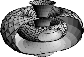
Figure 3: The $(X^{1},X^{2},X^{3})$ axis are chosen in accordance with a right-handed coordinate system.

4.2 The Archimedes Map

The Archimedes map [22] or the Lambert projection [23] as it is sometimes called from $S^{2}$ to the cylinder over its equatorial circle provides a simple geometric explanation of the Wu-Yang construction and the field equation in terms of area and arclength. The Archimedes map

$${\mathcal{A}}(x,y,z)=\left(\frac{r}{\sqrt{r^{2}-z^{2}}}\,x,\,\,\frac{r}{\sqrt{r^{2}-z^{2}}}\,y,\,\,z\right),$$ (74)

is shown in Figure 4 $[(x^{1},x^{2},x^{3})\longrightarrow(x,y,z)]$. Choose a point $P$, except the poles, on $S^{2}$ and draw a straight line perpendicular to the axis of the cylinder which passes through $P$. The image of $P$ is defined as the point of intersection of this line with the cylinder. This yields $z=(1/\nu)\cos(\nu\theta)$ and $\phi$ denotes the length of arcs on parallels of the cylinder. This map is area preserving.

Figure 4: The Archimedes map is area preserving.

Consider two spherical caps $D_{N}$ and $D_{S}$ which are determined by the parallel $z$ respectively around the north and the south poles. The images of $D_{N}$ and $D_{S}$ are respectively given by the cylindrical regions $C_{N}$ and $C_{S}$. The area of a very small region on the sphere is given by the $2$-form $s=\sin(\nu\theta)d\theta\wedge d\phi$. The $1$-forms

$$a^{N}=\frac{1}{\nu}[1-\cos(\nu\theta)]d\phi\hskip 14.22636pt,\hskip 14.22636pta^{S}=-\frac{1}{\nu}[1+\cos(\nu\theta)]d\phi,$$ (75)

respectively yield the area $2$-form $s^{N}=s^{S}=s$ over $D_{N}$ and $D_{S}$: $s^{N}=da^{N}$, $s^{S}=da^{S}$. The area of the corresponding region on the cylinder is given by $h=-dz\wedge d\phi$. Then $h^{N}=db^{N}$, $h^{S}=db^{S}$ where

$$b^{N}=\left(\frac{1}{\nu}-z\right)d\phi\hskip 14.22636pt,\hskip 14.22636ptb^{S}=-\left(\frac{1}{\nu}+z\right)d\phi.$$ (76)

Here $b^{N}$ is the area of the vertical strip between the parallels $z=1/\nu$ and $z=(1/\nu)\cos(\nu\theta)$ of height $k^{N}=(1/\nu)-z$ and base length $d\phi$. Meanwhile $-b^{S}$ is the area of the vertical strip between the parallels $z=(1/\nu)\cos(\nu\theta)$ and $z=-1/\nu$ of height $k^{S}=(1/\nu)+z$ and base $d\phi$. The area of $D_{N}$ and $D_{S}$

$$S^{N}=\int_{D_{N}}s^{N}=\oint_{\partial D_{N}:P[\theta]}a^{N}\hskip 14.22636pt,\hskip 14.22636ptS^{S}=\int_{D_{S}}s^{S}=-\oint_{\partial D_{S}:P[\theta]}a^{S}$$

$$\hskip 19.91692pt=2\pi\frac{1}{\nu^{2}}\left[1-\cos(\nu\theta)\right]\hskip 65.44133pt=2\pi\frac{1}{\nu^{2}}\left[1+\cos(\nu\theta)\right]$$

$$\hskip 19.91692pt=2\pi\frac{1}{\nu}\left(\frac{1}{\nu}-z\right)\hskip 91.04881pt=2\pi\frac{1}{\nu}\left(\frac{1}{\nu}+z\right),$$ (77)

are respectively equal to the area of the regions $C_{N}$ and $C_{S}$. These are respectively given by the area of the rectangles with base $2\pi(1/\nu)$ and height $k^{N}$ and $k^{S}$.

The Wu-Yang solution is based on pasting the caps $D_{N}$ and $D_{S}$ along the common boundary $P:z(\theta)$. We need a dimensionful factor: $\nu^{2}/2g$ for the sake of dimensional consistency: $F=(\nu^{2}/2g)s$, $A^{N}=(\nu^{2}/2g)a^{N}$, $A^{S}=(\nu^{2}/2g)a^{S}$ and $Q^{N}=(\nu^{2}/2g)S^{N}$, $Q^{S}=(\nu^{2}/2g)S^{S}$. The gauge transformation formula (57) yields $U=\exp[i(2\phi/\nu)\nu^{2}/2]$ where the factor $2\phi/\nu$ is the area of a vertical strip of height $2/\nu$ and base $\phi$ on the cylinder. This leads to $U=\exp(igQ)$ where $Q=(4\pi/\nu^{2})\nu^{2}/2g$, in terms of the total area of the sphere or the cylinder. The $1$-forms $*F^{N}$ and $*F^{S}$ are given as: $*F^{N}=\nu A^{N}$, $*F^{S}=\nu A^{S}$. These yield $\Phi^{N}=\pi(\nu^{2}/g)k^{N}$, $\Phi^{S}=\pi(\nu^{2}/g)k^{S}$. Thus we can interpret the integrated field equations (62) simply as the area formula: $height=(1/base)area$ of a rectangle of height $k$ and base $2\pi/\nu$ up to an overall factor of $\nu^{2}/2g$

The quantization of the topological mass: $\nu=ng^{2}$ can be interpreted as division of the rectangle with base $2\pi/g^{2}$ and height $2/g^{2}$ into $n^{2}$ similar sub-rectangles of equal area.

4.3 The Geometric Phase

The analogy between the Berry phase [24], which corresponds to holonomy in a line bundle [25], and the magnetic monopole is well known, [26, 27], [29, 30, 31, 32], [33], [34]. The classical example of this is the geometric phase suffered by a vector upon parallel transport along the lattitude $\theta$ on the $2$-sphere [23], [28]. We can express this geometric phase in terms of holonomy of the topologically massive gauge potential or the dual-field.

Consider a vector $X$ which is tangent to $S^{2}$ at longitude $\phi=0$ and latitude $\theta$ as shown in Figure 5. If we parallel transport this vector along the latitude, after a complete revolution, it suffers a phase $\gamma$ which is determined by the solid angle $\Omega$ subtented by the parallel $P$ at latitude $\theta$ in $S^{2}$ [24], [29, 30, 31, 32], [34]. This is given as

$$\gamma_{N}=-\Omega_{N}\hskip 71.13188pt,\hskip 42.67912pt\gamma_{S}=\Omega_{S}$$

$$\hskip 17.07164pt=-2\pi[1-\cos(\nu\theta)]\hskip 71.13188pt=2\pi[1+\cos(\nu\theta)],$$

using the arclength parameterization. Note that $\gamma_{N}-\gamma_{S}=-4\pi$ although $\gamma_{N}\neq\gamma_{S}$. It is straightforward to verify this by solving the equation for parallel transport $\nabla_{(\phi)}X=0$ with the metric (18) on $S^{2}$ [28]. This equation reduces to

$$\frac{dZ}{d\phi}+i\nu\cos(\nu\theta)Z=0,$$ (79)

[23]. We find

$$Z(2\pi\frac{1}{\nu})=Z(0)\exp\{-i\oint_{P}\nu[1-\cos(\nu\theta)]d\phi\},$$ (80)

for a complete revolution. Here $Z(0)$ and $Z(2\pi/\nu)$ respectively correspond to the initial and the final vectors $X_{i}$, $X_{f}$. The phase in (80) reduces to the solid angle in (4.3) which is subtented by the parallel $P$ via the Stokes theorem.

Figure 5: The geometric phase $\tilde{\gamma}$ suffered by a vector $X$ upon parallel transport along the latitude $P:\theta$ is determined by the solid angle $\tilde{\Omega}$.

The phases (4.3) can be written in terms of holonomy $\Gamma$ of the topologically massive gauge potential or the dual-field over the parallel $P$ as

$$\gamma_{N}=-2\Gamma_{N}\hskip 42.67912pt,\hskip 42.67912pt\gamma_{S}=-2\Gamma_{S},$$ (81)

where

$$\Gamma_{N}=Q^{N}=\frac{1}{\nu}\Phi^{N}\hskip 42.67912pt,\hskip 42.67912pt\Gamma_{S}=-Q^{S}=-\frac{1}{\nu}\Phi^{S},$$ (82)

(3.4) and the factor $1/g$ is ignored. Here $\Gamma_{N}-\Gamma_{S}=2\pi$. The phase factors corresponding to holonomy of the sections $\tilde{A}^{N}$, $\tilde{A}^{S}$ of the potential (70) are equal

$$\exp(i\Gamma_{N})=\exp(i\Gamma_{S}),$$ (83)

since $p=1+k$ is an integer.

5 The Quantization of Topological Mass

If the strength of the potentials $A^{N}$, $A^{S}$ (3.2) were $\pm(1/2)mg$ then the gauge function would be $U=\exp{(img^{2}\phi)}=\exp{(ip\nu\phi)}$, see section $3.5$. This would yield $U=\exp{(i2\pi mg^{2}/\nu)}$ in terms of the total magnetic and electric charges $\Phi=\nu Q=2\pi mg$.

The expression $U=\exp{(i2\pi mg^{2}/\nu)}=\exp{(i2\pi p)}$ implies $\nu=ng^{2}$ with $p=\frac{m}{n}=1+k$ an integer. Hence $m$ is quantized in units of $n$. Here $p$ is the winding number of the gauge transformation which corresponds to the negative of the first Chern number. Thus the arclength parameterization leads to $r=1/ng^{2}$. Then $U=\exp{(img^{2}\phi)}$ is single-valued on this circle. Because as $\nu\phi\rightarrow\nu\phi+2\pi$

$$U=\exp{(img^{2}\phi)}\longrightarrow\exp{(i2\pi p)}\exp{(img^{2}\phi)}\hskip 8.53581pt,\hskip 14.22636ptm=pn,$$ (84)

since $0\leq\nu\phi\leq 2\pi$. More generally, $U\rightarrow\exp{(i2\pi pl)}U$ as $\nu\phi\rightarrow\nu\phi+2\pi l$ where $l$ is an integer. Then $l^{\prime}=pl$ is an integer too. Note that this discussion implicitly amounts to a redefinition of the arclength: $\phi\rightarrow p\phi$ without changing the length scale defined by $\nu$.

Further we require $U=\exp{(img^{2}\phi)}$ to be a single-valued function of $\phi$ independent of any a priori choice of a scale of length, neither by redefining the arclength $\phi$ nor by imposing the condition $0\leq\phi\leq L=2\pi/\nu$ on it. The identification $r=1/ng^{2}$ provides a fundamental unit of length $1/g^{2}$ or $\lambda=2\pi/g^{2}$ over which any gauge function is single-valued. Then as $g^{2}\phi\rightarrow g^{2}\phi+2\pi$

$$U=\exp{(img^{2}\phi)}\longrightarrow\exp{(i2\pi m)}\exp{(img^{2}\phi)},$$ (85)

since $0\leq g^{2}\phi\leq 2\pi$. This yields an integer value for $m$. More generally, $U\rightarrow\exp{(i2\pi mk)}U$ as $g^{2}\phi\rightarrow g^{2}\phi+2\pi k$ where $k$ is an integer. Then $l^{\prime}=mk$ is an integer too. This leads to the quantization of the topological mass. Because if $m=pn$ is an integer for any integer $p$ then $n$ is an integer too. The converse is also true.

Thus the quantization of topological mass further requires that the circle of perimeter $L=2\pi/\nu$ has been wound $n$ times by the fundamental circle of perimeter $\lambda$ with locally invariant arclength. This leads to $l=nk$ which yields $l^{\prime}=pl=mk$. More precisely, as $\phi$ changes from $\phi=0$ to $\phi=lL=l(\lambda/n)$ this circle is traversed $l$ times. Meanwhile, the fundamental circle is traversed $k=l/n$ times. If $k$ is an integer, then $l=nk$ is an integer if and only if $n$ is an integer too. Thus the fundamental circle covers this an integer $(l=)n$ times and its radius is $r=\lambda/(2\pi n)=1/ng^{2}$. The quantization of topological mass amounts to a discrete change of scale which arises from a winding by the circle of fundamental size with invariant arclength. Intuitively number $n$ is a measure of the topological thickness of the winding as the name topological mass suggests.

We can see this if we rewrite $\nu=ng^{2}$ as

$$\frac{\lambda}{{2\pi\frac{1}{\nu}}}=n.$$ (86)

Then the gauge function $U=\exp{(i\nu\phi)}$ is given as

$$U=\exp{(i\frac{2\pi n}{\lambda}\phi)}.$$ (87)

If $U$ is a single-valued function of $\phi$ with the fundamental length scale $\lambda$ for any $n$ then $n$ has to be an integer. The fundamental length scale $\lambda=nL$ is the least common multiple of intervals over which the gauge function is single-valued and periodic for any integer $n$ in addition to the fact that it has a smaller period $L=\lambda/n$ [19].

In other words the quantization of topological mass reduces to quantization of the inverse natural length scale in units of the inverse fundamental scale. We can associate the integer $n$ with a winding number of mapping of circles using the arclength parameterization.

In the fundamental units: $g=1$ the arclength $\phi$ reduces to angle: $0\leq\phi\leq 2\pi$ and the topological mass becomes $\nu=n$. One could identify the number $n$ with the topological winding number $p$ ignoring the physical dimensions and discuss the quantization of topological mass. If $U=\exp{(i\nu\phi)}$ is single-valued on the unit circle then $n$ is an integer.

5.1 The Winding Numbers

The Hopf map (3.2) defines a $S^{1}$ bundle over $S^{2}$ with a natural scale of length determined by the topological mass. The gauge function, that is the transition function of the bundle is given by a map $h:S^{1}_{(2)}\longrightarrow{S^{\prime}}^{1}_{(2)}$ from the equator $S^{1}_{(2)}=U_{N}\bigcap U_{S}$ of $S^{2}$ to the manifold of the gauge group ${S^{\prime}}^{1}_{(2)}$ [54]. The group $U(1)$ is given by normalizing the radius of ${S^{\prime}}^{1}_{(2)}$. Topological structure of the bundle is determined by homotopy class of the transition function which is characterized by the winding number of $S^{1}_{(2)}$ about ${S^{\prime}}^{1}_{(2)}$ [54, 57]. This winding number, which is associated with the magnetic charge of the monopole, corresponds to the negative of the First Chern number of the bundle. Meanwhile the size of ${S^{\prime}}^{1}_{(2)}$ (also $S^{1}_{(2)}$) is determined by a winding $f:S^{1}_{(1)}\longrightarrow{S^{\prime}}^{1}_{(2)}$ of the circle of fundamental size with locally invariant arclength.

The winding number of a map $u:\tilde{S}^{1}_{(1)}\longrightarrow\tilde{S}^{1}_{(2)}$ is defined as the degree of this map

$$\oint_{\tilde{S}^{1}_{(1)}}u^{*}(\omega_{(2)})=deg(u)\oint_{\tilde{S}^{1}_{(2)}}\omega_{(2)},$$ (88)

[59, 62, 63]. Here $\omega_{(2)}$ is the arclength $1$-form on $\tilde{S}^{1}_{(2)}$ and $u^{*}(\omega_{(2)})$ is its pull-back onto $\tilde{S}^{1}_{(1)}$. The map $u$ is uniquely defined for each point in $\tilde{S}^{1}_{(1)}$ and it is single-valued in $\tilde{S}^{1}_{(2)}$ if and only if the degree $deg(u)$, which measures the effective number $\tilde{S}^{1}_{(2)}$ is covered by $\tilde{S}^{1}_{(1)}$, is an integer. Note that this definition is independent of choice of a length scale. In the non-massive case, which has no natural scale, this map is defined only in terms of angles. In the present case we use arclength parameterization for defining this in accordance with the natural scale of length.

The gauge function $U$ is given by $h:S^{1}_{(2)}\longrightarrow{S^{\prime}}^{1}_{(2)}$

$$\exp(i\nu\phi^{\prime}_{(2)})=\exp(ip\nu\phi_{(2)}),$$ (89)

where the circles $S^{1}_{(2)}$ and ${S^{\prime}}^{1}_{(2)}$ are of the same radius $r^{\prime}_{(2)}=r_{(2)}=1/\nu$. Then $\phi^{\prime}_{(2)}=p\phi_{(2)}$ while $\tilde{\phi}^{\prime}_{(2)}=p\tilde{\phi}_{(2)}$. We find

$$deg(h)=p,$$ (90)

since $r_{(2)}/r^{\prime}_{(2)}=1$ (88). Hence, as $S^{1}_{(2)}$ is traversed $l$ times, ${S^{\prime}}^{1}_{(2)}$ is traversed $l^{\prime}=pl$ times. Note that $deg(h)=p$ is independent of choice of any length scale $r^{\prime}_{(2)}=r_{(2)}$.

Consider the function $g:S^{1}_{(1)}\longrightarrow S^{1}_{(2)}$

$$\hskip 28.45274pt\exp(i\nu\phi_{(2)})=\exp(in\nu_{(1)}\phi_{(1)}),$$ (91)

which maps the circle $S^{1}_{(1)}$ onto $S^{1}_{(2)}$ with locally invariant arclength $\phi_{(2)}=\phi_{(1)}$ where $\nu_{(1)}=1/g^{2}$. Then $r_{(1)}=nr_{(2)}$ and $\lambda=nL$ while $\tilde{\phi}_{(2)}=n\tilde{\phi}_{(1)}$. The degree formula (88) yields the winding number as the ratio $r_{(1)}/r_{(2)}$

$$deg(g)=n.$$ (92)

Hence, as $S^{1}_{(1)}$ is traversed $k$ times, $S^{1}_{(2)}$ is traversed $l=nk$ times. The radius $r_{(2)}$ of circle $S^{1}_{(2)}$ is determined by the winding number $n=r_{(1)}/r_{(2)}$.

The composite mapping $f=h\cdot g$ is given as

$$\exp(i\nu\phi^{\prime}_{(2)})=\exp(im\nu_{(1)}\phi_{(1)}).$$ (93)

In this case $\phi^{\prime}_{(2)}=p\phi_{(1)}$ while $\tilde{\phi}^{\prime}_{(2)}=m\tilde{\phi}_{(1)}$ since $r_{(1)}=nr^{\prime}_{(2)}$, $m=np$. The degree formula (88) yields the winding number as the product

$$deg(f)=m.$$ (94)

Then as $S^{1}_{(1)}$ is traversed $k$ times, ${S^{\prime}}^{1}_{(2)}$ is traversed $l^{\prime}=mk$ times. This is equivalent to the case in $g$. That is, $m=np$ is an integer for any integer $p$ if and only if $n$ is an integer too. We find $m=n$ for $p=1$ while $m=p$ for $r_{(1)}/r_{(2)}=n=1$.

5.2 Dirac Quantization Condition

We can now elucidate the acclaimed relation between the quantization of topological mass and Dirac quantization condition [36, 37]. Consider Dirac potentials $A^{N/S}$ of magnetic strength $g^{\prime}$ on the respective charts $U_{N/S}$ of $S^{2}$ with radius $r=1/\nu$

$$A^{N/S}=\pm\frac{1}{2}g^{\prime}\nu\left[1\mp\cos(\nu\theta)\right]d\phi=\pm\frac{1}{2}n^{\prime}\frac{\nu}{g}\left[1\mp\cos(\nu\theta)\right]d\phi,$$ (95)

where $gg^{\prime}=n^{\prime}$. The relations $gg^{\prime}=n^{\prime}$ and $\nu=ng^{2}$ yield $\nu g^{\prime}=sg$ [37], $s=nn^{\prime}$. The magnetic and electric charges associated with the potentials $A^{N/S}$ are

$$Q^{N/S}=2\pi g^{\prime},\hskip 28.45274pt \Phi^{N/S}=2\pi g^{\prime}\nu=2\pi sg.$$ (96)

The potentials $A^{N/S}$ differ by a gauge transformation $U=\exp(igg^{\prime}\nu\phi)$. The Wu-Yang construction yields the gauge function as $U=\exp(i2\pi gg^{\prime})$ in terms of the magnetic or electric charges. Thus $gg^{\prime}=n^{\prime}$ or equivalently $p^{\prime}=n^{\prime}$ $(p=1)$ is an integer. If $m^{\prime}=s$ is to be an integer as described above then $n$ is an integer too.

6 Conclusion

We have considered euclidean Wu-Yang type solutions of the MCS and the $SU(2)$ YMCS theories on the dS space $S^{3}$. We have discussed the introduction of a physical scale of length determined by the inverse topological mass $\nu\sim ng^{2}$ in these solutions from a geometrical point of view. We have embedded the abelian solution into the YMCS theory by means of a $SU(2)$ gauge transformation which has winding number $w=1$. The total action for this solution only consists of the YM piece. The action for the abelian solution vanishes.

In the abelian case the field locally determines the potential up to a closed $1$-form via the self-duality equation. We have introduced a transformation of the gauge potential using the dual-field strength which can be identified with a gauge transformation.

Then we have discussed the Hopf map $S^{3}\longrightarrow S^{2}$ including the topological mass. This has led to a reduction of the field equation onto $S^{2}$ using local sections of $S^{3}$. The Hopf map has given rise to the local potentials on $S^{2}$ which differ by a gauge transformation. These solutions have a composite structure consisting of both magnetic and electric charges because of the local character of the field equation. The quantization of the total electric charge $\Phi$ requires the quantization of the topological mass.

This has naturally led to the Wu-Yang solution which is based on seaming the local potentials across the common boundary by means of a gauge transformation. The gauge function can be expressed in terms of either the magnetic or the electric charges. We have also presented abelian solutions with different first Chern numbers.

We have also presented three geometric structures which arise in connection with our solutions. We have presented a stereographic view of the fibers in the Hopf map. The Archimedes map has provided a simple picture for the Wu-Yang solution. This has led to a simple interpretation of the composite structure in terms of the area of a rectangle. We have also expressed the geometric phase suffered by a vector upon parallel transport on $S^{2}$ in terms of the holonomy of the topologically massive gauge potential or the dual-field.

Then we have discussed quantization of the topological mass $\nu=ng^{2}$ in the abelian case. In geometric terms, quantization of the topological mass reduces to quantization of inverse of the natural scale of length $L=2\pi/ng^{2}$ in units of the inverse of the fundamental length scale $\lambda=2\pi/g^{2}$. The fundamental length scale $\lambda$ is the least common multiple of intervals over which the gauge function is single-valued and periodic for any integer $n$ in addition to the fact that it has a smaller period $L=\lambda/n$. The number $n$ can be identified with the winding number of a function that maps the circle of fundamental size about this circle with locally invariant arclength. Meanwhile the First Chern number is given by the winding number of maps of circles of the same size $L$. We have also discussed Dirac quantization condition.

Finally, we would like to point out a naive analogy between the natural length scale introduced by the topological mass and the Hall resistivity $R=1/ng^{2}$. The monopole/instanton type solutions presented here might provide a geometrical explanation for the levels if the particles in the Hall effect gave rise to a gauge theoretic system with a fundamental length scale $1/g^{2}$. An immediate prediction would be the effect of quenching if the sample size is of the order of radius of these particles’ orbits, while the smaller orbits survived.

We remark that the most distinctive feature of the topologically massive gauge theories is the existence of a natural scale of length introduced by the topological mass. We have demonstrated that incorporation of this crucial fact which was ignored in the literature, settles down the physical discussions into a consistent geometric frame. To the knowledge of the author, the solutions and geometric constructions presented here which clarify this issue are lacking in the literature.

References

• [1] S. Deser, R. Jackiw, S. Templeton, Phys. Rev. Lett., 48 (1982), 975.
• [2] S. Deser, R. Jackiw, S. Templeton, Ann. Phys., 140 (1982), 372.
• [3] J. F. Schonfeld, Nuc. Phys. B, 185 (1981), 157.
• [4] S. Deser, Phys. Rev. Lett., 64 (1990), 611.
• [5] R. Jackiw in โ€œRelativity, Groups and Topology IIโ€, (Les Houches Session XL, 1983, ed. B. DeWitt, R. Stora), North-Holland, 1984.
• [6] P. Goddard, D. I. Olive, Rep. Prog. Phys., 41 (1978), 1357.
• [7] A. N. Aliev, Y. Nutku, K. Saygili, Class. Quant. Grav., 17 (2000), 4111.
• [8] C. N. Yang, Phys. Rev. Lett., 33 (1974), 445.
• [9] T. T. Wu, C. N. Yang, Phys. Rev. D, 12 (1975), 3845.
• [10] L. H. Ryder, โ€œQuantum Field Theoryโ€, Cambridge University Press, 2006.
• [11] P. K. Townsend, K. Pilch, P. Van Nieuwenhuizen, Phys. Lett. B, 136 (1984), 38.
• [12] S. Deser, R. Jackiw, Phys. Lett. B, 139 (1984), 371.
• [13] T. T. Wu, C. N. Yang, Phys. Rev. D, 12 (1975), 3843.
• [14] M. Minami, Prog. Theor. Phys., 62 (1979), 1128.
• [15] L. H. Ryder, J. Phys. A, Math. Gen., 13 (1980), 437.
• [16] A. Trautman, Int. Jour. Theor. Phys., 16 (1977), 561.
• [17] S. Mandelstam, Phys. Rev. D, 19 (1979), 2391.
• [18] K. G. Wilson, Phys. Rev. D, 10 (1974), 2445.
• [19] R. Penrose, โ€œThe Road to Realityโ€, A. A. Knopf, 2005.
• [20] M. Berger, โ€œGeometryโ€, Springer-Verlag, 2004.
• [21] W. P. Thurston, โ€œThree-Dimensional Geometry and Topologyโ€, Princeton University Press, 1997.
• [22] D. McDuff, D. Salamon, โ€œIntroduction to Symplectic Topologyโ€, Clarendon Press, Oxford, 1998.
• [23] I. Agricola, T. Friedrich, โ€œGlobal Analysis, Differential Forms in Analysis, Geometry and Physicsโ€, Graduate Studies in Mathematics 52, Americal Mathematical Society, 2002.
• [24] M. V. Berry, Proc. R. Soc. Lond., A, 392 (1984), 45.
• [25] B. Simon, Phys. Rev. Lett., 51 (1983), 2167.
• [26] B. Zumino, preprint, UCB/PTH-87/13.
• [27] E. Kritsis, preprint, CALT-68-1336.
• [28] M. Nakahara, โ€œGeometry, Topology and Physicsโ€, IOP Publishing Ltd., 1996.
• [29] J. H. Hannay, J. Phys. A, 18 (1985), 221.
• [30] J. Anandan, L. Stodolsky, Phys. Rev. D., 35 (1987), 2597.
• [31] H. Li, Phys. Rev. D, 35 (1987), 2615.
• [32] M. G. Benedict, L. Gy. Feher, Z. Horvath, J. Math. Phys., 30 (1989), 1727.
• [33] I. J. J. Aitchison, Acta Physica Polonica B, 18 (1987), 207.
• [34] A. Mostafazadeh, โ€œDynamical Invariants, Adiabatic Approximation and the Geometric Phaseโ€, Nova Science Publishers, Inc., 2001.
• [35] O. Alvarez, Commun. Math. Phys., 100 (1985), 279.
• [36] A. P. Polychronakos, Nuc. Phys. B, 281 (1987), 241.
• [37] M. Henneaux, C. Teitelboim, Phys. Rev. Lett., 56 (1986), 689.
• [38] P. A. Horvathy, C. Nash, Phys.Rev. D, 33 (1986), 1822.
• [39] R. D. Pisarski, Phys. Rev. D, 34 (1986), 3851.
• [40] I. Affleck, J. Harvey, L. Palla, G. Semenoff, Nucl. Phys. B, 328 (1989), 575.
• [41] R. Jackiw, S.-Y. Pi, Phys. Lett. B, 423 (1998), 364.
• [42] B. Tekin, K. Saririan, Y. Hosotani, Nucl. Phys. B, 539 (1999), 720.
• [43] K. Saygili, Int. Jour. Mod. Phys. A, 22 (2007), 2961.
• [44] . K. Saygili, Int. Jour. Mod. Phys. A, to be published.
• [45] B. Hou, B. Hou, โ€œDifferential Geometry for Physicistsโ€, World Scientific, 1997.
• [46] S. Bhagavantam, T. Venkatarayudu, โ€œTheory of Groups and its Application to Physical Problemsโ€, Academic Press, 1969.
• [47] K. Gottfried โ€œQuantum Mechanics, Volume 1: Fundamentalsโ€, W. A. Benjamin Inc, New York, 1966.
• [48] N. Itzhaki, Phys. Rev. D, 67 (2003), 065008.
• [49] S. Deser, in โ€œDirections in General Relativityโ€, vol.2, p.114, College Park 1993.
• [50] S. Deser, R. Jackiw, Phys. Lett. B, 451 (1999), 73.
• [51] M. A. M Gomes, R. R. Landim, J. Phys. A: Math. Gen. 38 (2005), 257.
• [52] V. E. R. Lemes, C. Linhares de Jesus, C. A. G. Sasaki, S. P. Sorella, L. C. Q. Vilar, O. S. Ventura, Phys. Lett. B, 418 (1998), 324.
• [53] V. E. R. Lemes, C. Linhares de Jesus, S. P. Sorella, L. C. Q. Vilar, O. S. Ventura, Phys. Rev. D, 58 (1998), 045010.
• [54] J. A. De Azcarraga, J. M. Izquierdo, โ€œ Lie groups, Lie algebras, cohomology and some applications in physicsโ€, Cambridge University Press, 1998.
• [55] V. A. Vassiliev, โ€œIntroduction to Topologyโ€, Student Mathematical Library 14, American Mathematical Society, 2001.
• [56] M. Spivak, โ€œA Comprehensive Introduction to Differential Geometryโ€, Publish or Perish Inc., 1999.
• [57] N. Steenrod, โ€œThe Topology of Fibre Bundlesโ€, Princeton University Press, 1951.
• [58] R. Bott, L. W. Tu, โ€œDifferential Forms in Algebraic Topologyโ€, Springer-Verlag, 1982.
• [59] W. Greub, S. Halperin, R. Vanstone, โ€œConnections, Curvature, and Cohomologyโ€, volume 1, 2, Academic Press Inc. 1972, 1973.
• [60] A. D. Popov, Jour. Math. Phys., 46 (2005), 073506.
• [61] T. Eguchi, P. B. Gilkey, A. J. Hanson, Phys. Rep., 66 (1980), 213.
• [62] B. Felsager, โ€œGeometry, Particles, and Fieldsโ€, Springer-Verlag, 1998.
• [63] I. Madsen, J. Tornehave, โ€œFrom Calculus to Cohomologyโ€, Cambridge University Press, 1997.