Universal regularization for string field theory

Abstract:

We find an analytical regularization for string field theory calculations. This regularization has a simple geometric meaning on the worldsheet, and is therefore universal as level truncation. However, our regularization has the added advantage of being analytical. We illustrate how to apply our regularization to both the discrete and continuous basis for the scalar field and for the bosonized ghost field, both for numerical and analytical calculations. We reexamine the inner products of wedge states, which are known to differ from unity in the oscillator representation in contrast to the expectation from level truncation. These inner products describe also the descent relations of string vertices. The results of applying our regularization strongly suggest that these inner products indeed equal unity. We also revisit Schnabl’s algebra and show that the unwanted constant vanishes when using our regularization even in the oscillator representation.

1 Introduction

Regularization should be made with care for issues such as symmetries, analyticity and the origin of divergences. One amusing example is given by regularizing the bosonic and fermionic contributions to the vacuum energy in the context of the DBI action [1, 2]. In both cases one gets an infinite set of constant contributions, but they should be regularized differently since they originate from integer and half-integer modes respectively. For the bosonic case one gets

$$\sum_{n=1}^{\infty}1\equiv\zeta(0)=-\frac{1}{2}\,,$$ (1)

while for the fermionic case

$$\sum_{n=\frac{1}{2}}^{\infty}1\equiv\zeta(0,\frac{1}{2})=0\,.$$ (2)

In this paper we address the issue of regularization in bosonic string field theory [3]. Here, divergences can occur due to the singular nature of the string vertices that act as delta functionals. Witten addressed these divergences by defining the delta functionals using strips with finite width in the limit where this width tends to zero. Witten’s construction was made more explicit using oscillators [4, 5, 6, 7, 8] and CFT methods [9, 10]. All these methods give expressions for Witten’s vertex with strips of zero width.

Actually, it turns out that usually no regularization is required as long as we do not care about the overall normalization. In cubic string field theory only the two- and three-vertices are needed, and since the two-vertex has trivial normalization, any non-trivial normalization of the three-vertex can be absorbed into field redefinitions.

Yet, this is not always the case, since in practice, other vertices are also used. The most prominent example is Schnabl’s analytic solution to the equation of motion [14]. In this work, Schnabl constructed the solution using a novel gauge and proved Sen’s first conjecture [15, 16]. Following his construction the consistency of the solution was verified [17, 18] and Sen’s third conjecture was proven [19]. Generalizations of his construction for the toy model introduced in [20] and exploration of their geometric meaning were presented in [21]. A continuous basis oscillator representation for Schnabl’s operators was found in [22] and a study of scattering amplitudes in a variation of his gauge was performed in [23].

Schnabl’s construction uses an infinite sum of wedge states. Wedge states are surface states that are naturally related to string vertices [24, 25, 26, 27]. For integer $n$ the wedge state $\left|n\right>$ can be defined as the contraction of the $n$ string field vertex $\left|V_{n}\right>$ with $n-1$ vacua. While Schnabl’s universal construction is safe from normalization anomalies, they can occur when working with an explicit CFT. Indeed, when choosing to work with 26 scalar fields plus the bosonized ghost, all represented in the continuous basis, an anomaly occurs in the algebra of Schnabl’s operators [22]. This should be interpreted as an artifact, stating that the regularization procedure used is anomalous.

Another, even more called for example of such an anomaly comes from evaluating the descent relation among string field vertices $\left<V_{1}\vphantom{V_{3}}\right|\left.\!\vphantom{V_{1}}{V_{3}}\right>=\left|V_{2}\right>$ or the analogous equation with wedge states $\left<1\vphantom{3}\right|\left.\!\vphantom{1}{3}\right>=1$. One gets the second equation from the first upon contraction with two vacuum states with ghost numbers zero and three. The first evaluation of this expression in the oscillator representation was attempted in the continuous basis [28, 29, 30, 31, 32]. There, it was found that the result of the inner product is not unity. In order to identify the source of this problem, numerical evaluations of these expressions using oscillator level truncation in the discrete basis were performed in [35, 36]. These papers illustrated that the problem is not related to the use of the continuous basis.

In the seminal paper of LeClair, Peskin and Preitschopf [10] a formal justification for the descent relations was given. It relied on the fact that the relation

$$\left<0\right|\exp\Big{(}{\sum_{n=0}^{\infty}v_{n}L_{n}}\Big{)}\exp\Big{(}{\sum_{n=0}^{\infty}u_{n}L_{-n}}\Big{)}\left|0\right>=1\,,$$ (3)

holds as long as $v_{n},u_{n}$ are small enough and the total central charge is zero. One criterion to check whether $v_{n},u_{n}$ are indeed small enough is to turn on a central charge. If the above correlator diverges, it could be a sign of trouble. Unfortunately, it diverges in the case of the vertices. This raises the question of whether we can trust the descent relations

$$\left<V_{1}\vphantom{V_{N}}\right|\left.\!\vphantom{V_{1}}{V_{N}}\right>=\left|V_{N-1}\right>,$$ (4)

or is it necessary to add some normalization factors to these relations. In this paper we find an analytical regularization under which these relations hold.

The apparent validity of (3) is a direct consequence of the Virasoro algebra with zero central charge. This suggest that any universal regularization should work. Universality refers here to independence of the choice of CFT, as long as the total system has a vanishing central charge.

The regularization we suggest is to shrink the string field states using the conformal map $f_{s}(\xi)=s\xi$, where $\xi$ is a coordinate on the upper half-plane with the half unit circle as the local coordinate patch and $s<1$ is the dilatation parameter. Geometrically this regularization can be viewed as reinstating Witten’s prescription of using a strip with half-width of $\log s^{-1}$, as can be seen in the $\tau,\sigma$ coordinates. This regularization respects the symmetry of the problem since it is universal by construction while resolving the origin of the singularity, i.e. the delta-functional gluing and the conical singularity of the string vertices, see figure 1.

Figure 1: The effect of the regularization on the canonical coordinate patch (a), the two-vertex (b) and the three-vertex (c).

Expanding a field $\Psi$ in level components $\Psi_{h}$, the regularized field can be expressed as

$$\Psi^{s}\equiv f_{s}\circ\Psi=s^{L_{0}}\Psi=\sum_{h}s^{h}\Psi_{h}\,.$$ (5)

This shows that our regularization is closely related to level truncation [37]. Specifically, writing

$$\left<\Psi_{1}^{s}\vphantom{\Psi_{2}^{s}}\right|\left.\!\vphantom{\Psi_{1}^{s}}{\Psi_{2}^{s}}\right>=g_{12}(s)\,,$$ (6)

one can obtain the level $(L,2L)$ result from Taylor expanding $g_{12}(s)$ to order $2L$ and then setting $s=1$. This also demonstrates the down side of level truncation. The function $g_{12}(s)$ can have a well defined Taylor expansion, but with radius of convergence less than unity. Calculations to any finite level will not yield a divergent result.

Our regularization has the added feature of analyticity, which is missing in level truncation. To demonstrate this we can look at the overlap of two butterfly states

$$\left<B_{\alpha}\vphantom{B_{\beta}}\right|\left.\!\vphantom{B_{\alpha}}{B_{\beta}}\right>=\left<0\right|\exp\Big{(}\frac{1}{2}\alpha L_{2}\Big{)}\exp\Big{(}\frac{1}{2}\beta L_{-2}\Big{)}\left|0\right>=(1-\alpha\beta)^{-\frac{c}{8}}.$$ (7)

This case is simple enough to derive the explicit normalization. Setting $\alpha=\beta$ we can calculate the normalization of the butterfly state. It is clear that for $|\alpha|>1$ the normalization is not well defined. Still, truncating to any finite level gives a finite result. Calculating the normalization in our regularization simply amounts to rescaling $\alpha\rightarrow s^{2}\alpha$. Notice, that even though the level truncation calculation simply amounts to repeatedly applying the Virasoro algebra, it is quicker to use our regularization and then Taylor expand the result. The limiting case $\alpha=1$ is the interesting case where the butterfly becomes a projector. The normalization is only well defined if we apply our regularization. Geometrically, in this case the boundary of the surface exactly pinches the coordinate patch (at the mid-point). Our regularization shrinks the state to avoid this singularity.

The effect of our regularization on squeezed states is simply to rescale its defining matrix and vector,

$$\left|S^{s}\right>=\exp(a^{\dagger}S^{s}a^{\dagger}+V^{s}a^{\dagger})\left|0\right>,\qquad S^{s}_{nm}=S_{nm}s^{n+m}\,,\quad V^{s}_{n}=V_{n}s^{n}\,.$$ (8)

This means that we can still use squeezed state techniques in our calculations, which are usually more efficient than level truncation calculations. Actually, many calculations in oscillators were done by truncating the matrix $S_{nm}$ to finite size. This method, named oscillator level truncation, can be used to harness the power of squeezed state techniques. In particular it was used in [38] for defining the spectral density of the continuous basis and in [39, 40] for calculating scattering amplitudes. However, as stated above, oscillator level truncation can give anomalous results. Normalization calculations in the continuous basis also suffer from the same inconsistencies. In this paper we show how to apply our regularization to the discrete basis and to the continuous basis and demonstrate that it gives consistent results in both cases.

To calculate the normalization of the descent relations (4) we contract them with $N-1$ vacuum states. This leaves us with two wedge states

$$\left<1\vphantom{N}\right|\left.\!\vphantom{1}{N}\right>\equiv\gamma_{1,N}\,.$$ (9)

Using (3) we get $\gamma_{1,N}=1$, but as we demonstrated with the butterfly calculation (7), one must use (3) with caution.

In this paper we analyze the more general wedge state inner product $\gamma_{n_{1},n_{2}}\equiv\left<n_{1}\vphantom{n_{2}}\right|\left.\!\vphantom{n_{1}}{n_{2}}\right>$ using our regularization. We show that $\gamma_{2+t_{1},2+t_{2}}=1+{\cal O}(t_{1}^{3}t_{2}^{3})$. We also prove that (the expression with the most potential for singularities) $\gamma_{1,1}=1$, and evaluate $\gamma_{1,3}$ numerically showing that it is consistent with being unity for values of $s$ at least up to $s=0.999$. This seems sufficient to claim that $\gamma_{n_{1},n_{2}}=1$ in the context of our regularization. We believe that the contraction of any two legitimate surface states, i.e. states whose defining surface contains the local coordinate patch, would give unity, when using our regularization.

Our regularization is for states. It can be generalized to operators, but only if one is careful to use it in the right context. The ambiguity comes from the fact that an operator of weight $h$ can be scaled as $s^{h}$ or $s^{-h}$ depending on whether it appears in a ket or a bra state. To avoid this ambiguity we limit the use of regularized operators to computations involving normal ordered states. Then creation operators will always appear in ket states while annihilation operators will always appear in bra states. There is a subtlety with the ghost zero-modes, which is resolved by acting on either of the vacua with the $c_{1},c_{0},c_{-1}$ ghost operators. This is needed to saturate the ghost number anomaly. Non unitary CFT’s, like the scalar field with time signature, are another issue. We will postpone the question of regularizing operators like $:e^{ikX}:$ to a later time. For now, we present a few examples. We start with the Virasoro operators. Under the above conditions the regularized Virasoro operators are

$$L_{n}^{s}=s^{|n|}L_{n}\,.$$ (10)

These operators satisfy the regularized Virasoro algebra

$$[L_{n}^{s},L_{m}^{s}]=s^{|n|+|m|-|n+m|}\left((n-m)L_{n+m}^{s}+\frac{c}{12}(n^{3}-n)\delta_{n+m}\right).$$ (11)

This algebra is guaranteed to satisfy the Jacobi identity by construction. For the scalar field we have (ignoring zero-modes)

$$\alpha_{n}^{s}=s^{|n|}\alpha_{n}\,,\qquad[\alpha_{n}^{s},\alpha_{m}^{s}]=s^{|2n|}n\delta_{n+m}\,.$$ (12)

In terms of these operators the Virasoro operators are

$$\qquad L_{n}^{s} =\frac{1}{2}\sum_{m=1}^{n-1}\alpha_{m}^{s}\alpha_{n-m}^{s}+\sum_{m=n+1}^{\infty}s^{2(n-m)}\alpha_{m}^{s}\alpha_{n-m}^{s} n>0\,,\qquad$$ (13)

$$\qquad L_{n}^{s} =\frac{1}{2}\sum_{m=n+1}^{-1}\alpha_{m}^{s}\alpha_{n-m}^{s}+\sum_{m=-\infty}^{n-1}s^{2(m-n)}\alpha_{m}^{s}\alpha_{n-m}^{s} n<0\,.\qquad$$ (14)

It might seem that these expressions diverge since we have negative powers of $s<1$, but one can check that in the dependence of $L_{n}^{s}$ on the original oscillators there are only positive powers of $s$.

The rest of the paper is structured as follows. In section 2 we show how to regularize continuous basis calculations. In section 3 we analyze Schnabl’s algebra using our regularization and generalizations thereof. In section 4 we calculate the descent relations in the continuous and in the discrete basis. We conclude in section 5.

2 The continuous basis

Our regularization is analytic with respect to $s$, unlike level truncation regularization, where the dependence on the level is encoded in a step-function. From (8), we see that for calculations involving squeezed states we should add, between every two contracted indices, the regularizing matrix

$$\rho_{s}^{nm}\equiv\delta_{n,m}s^{2n}\,.$$ (15)

However, we would also like to work in the continuous basis to get analytical expressions, whenever possible. To that end, we evaluate $\rho_{s}$ in the continuous basis in 2.1. Then, in 2.2 we illustrate the properties of the resulting expression.

2.1 Evaluating the form of the regulator in the continuous basis

The continuous basis is the basis that diagonalizes $K_{1}=L_{1}+L_{-1}$ [38]. The oscillators in this basis can be written as a linear combination of the discrete basis oscillators,

$$a^{\dagger}_{\kappa}=\sum_{n=1}^{\infty}\frac{v_{n}^{{\kappa}}}{\sqrt{{\cal N}({\kappa})}}\,a^{\dagger}_{n}\,,\qquad a_{\kappa}=\sum_{n=1}^{\infty}\frac{v_{n}^{{\kappa}}}{\sqrt{{\cal N}({\kappa})}}\,a_{n}\,,$$ (16)

where $-\infty<{\kappa}<\infty$. The transformation matrix is defined by the generating function,

$$f_{\kappa}(z)=\frac{1-e^{-{\kappa}\tan^{-1}z}}{{\kappa}}\equiv\sum_{n=1}^{\infty}\frac{v_{n}^{\kappa}}{\sqrt{n}}z^{n}\,.$$ (17)

The normalization,

$${\cal N}({\kappa}) =\frac{2}{{\kappa}}\sinh(\frac{{\kappa}\pi}{2})\,,$$ (18)

gives orthogonality and completeness relations of the form

$$\int_{-\infty}^{\infty}d{\kappa}\frac{v_{n}^{{\kappa}}v_{m}^{{\kappa}}}{{\cal N}({\kappa})}= \delta_{nm}\,,$$ (19)

$$\sum_{n=1}^{\infty}v_{n}^{{\kappa}}v_{n}^{{\kappa}^{\prime}}= {\cal N}({\kappa})\delta({\kappa}-{\kappa}^{\prime})\,.$$ (20)

We can write the regularizing matrix (15) in the continuous basis as

$$\rho_{\epsilon}({\kappa},{\kappa}^{\prime}) =\frac{1}{\sqrt{{\cal N}({\kappa}){\cal N}({\kappa}^{\prime})}}\sum_{n,m=1}^{\infty}v_{n}^{\kappa}v_{m}^{{\kappa}^{\prime}}\rho_{s}^{nm}=\frac{1}{\sqrt{{\cal N}({\kappa}){\cal N}({\kappa}^{\prime})}}\sum_{n=1}^{\infty}v_{n}^{\kappa}v_{n}^{{\kappa}^{\prime}}s^{2n}\,,$$ (21)

$${\epsilon} \equiv 1-s\,.$$ (22)

From the operator regularization point of view this matrix can be interpreted as the commutation relation

$$[a_{\kappa}^{s},{a_{{\kappa}^{\prime}}^{s}}^{\dagger}]=\rho_{\epsilon}({\kappa},{\kappa}^{\prime})\,.$$ (23)

This expression is reminiscent of the expressions that one gets in level truncation [28, 29, 30]. However, here the regularization matrix is non-diagonal and thus resolves the singular delta-type behaviour.

We can write the regularizing matrix explicitly using

$$\sum_{n=1}^{\infty}v_{n}^{\kappa}v_{n}^{{\kappa}^{\prime}}s^{2n}=\frac{s}{2}\partial_{s}\frac{1}{2\pi i}\oint\frac{du}{u}f_{\kappa}(u)f_{{\kappa}^{\prime}}\big{(}\frac{s^{2}}{u}\big{)}\,.$$ (24)

It is easy to see that only the term involving two exponents gives a non-zero result. Rescaling $u$ we get,

$$\sum_{n=1}^{\infty}v_{n}^{\kappa}v_{n}^{{\kappa}^{\prime}}s^{2n}=\frac{s}{2}\partial_{s}\frac{1}{2\pi i}\oint\frac{du}{u}\frac{e^{-{\kappa}\tan^{-1}(su)-{\kappa}^{\prime}\cot^{-1}(\frac{u}{s})}}{{\kappa}{\kappa}^{\prime}}\,.$$ (25)

We now take $u$ on the unit circle, where the integral is well defined for all $s<1$ and expand the argument around $s=1$,

$$\sum_{n=1}^{\infty}v_{n}^{\kappa}v_{n}^{{\kappa}^{\prime}}s^{2n}=-\frac{1-{\epsilon}}{4\pi{\kappa}{\kappa}^{\prime}}\partial_{\epsilon}\int_{0}^{2\pi}d\theta e^{-{\kappa}_{+}\tan^{-1}\left(\frac{\cos\vphantom{{}^{2}}\theta}{{\epsilon}}\left(1-\frac{{\epsilon}}{2}+{\cal O}({\epsilon}^{2})\right)\right)-i{\kappa}_{-}\tanh^{-1}\left(\sin\theta(1-\frac{{\epsilon}^{2}}{2})+{\cal O}({\epsilon}^{2})\right)},$$ (26)

where we define

$${\kappa}_{\pm}\equiv\frac{{\kappa}\pm{\kappa}^{\prime}}{2}\,.$$ (27)

We know from the derivation of the level-truncation expression $\rho_{\text{fin}}$ that this expression diverges as $\log{\epsilon}$. We are thus, not interested in ${\cal O}({\epsilon})$ corrections to the expression, because they would not contribute even for a product of regulators. We also note that the argument of the exponent is bounded. Thus, we can neglect higher order terms. Moreover, a rescaling of ${\epsilon}\rightarrow{\epsilon}(1+\frac{{\epsilon}}{2})$ gives,

$$\sum_{n=1}^{\infty}v_{n}^{\kappa}v_{n}^{{\kappa}^{\prime}}s^{2n}=-\frac{1}{4\pi{\kappa}{\kappa}^{\prime}}\partial_{\epsilon}\int_{0}^{2\pi}d\theta e^{-{\kappa}_{+}\tan^{-1}\left(\frac{\cos\theta}{{\epsilon}}\right)-i{\kappa}_{-}\tanh^{-1}\left(\sin\theta(1-\frac{{\epsilon}^{2}}{2})\right)}.$$ (28)

We now use the obvious symmetries and find that up to the relevant accuracy we have,

$$\rho_{\epsilon}({\kappa},{\kappa}^{\prime})=\frac{I_{1}+I_{2}}{\pi{\kappa}{\kappa}^{\prime}\sqrt{{\cal N}({\kappa}){\cal N}({\kappa}^{\prime})}}\,.$$ (29)

Here,

$$I_{1}=-\int_{0}^{\frac{\pi}{2}}\frac{{\kappa}_{-}{\epsilon}\sin\theta d\theta}{\cos^{2}\theta+{\epsilon}^{2}\sin^{2}\theta}\cosh\big{(}{\kappa}_{+}\tan^{-1}(\frac{\cos\theta}{{\epsilon}})\big{)}\sin\Big{(}{\kappa}_{-}\tanh^{-1}\big{(}(1-\frac{{\epsilon}^{2}}{2})\sin\theta\big{)}\Big{)}=$$

$$-\int_{0}^{1}\frac{{\kappa}_{-}{\epsilon}dx}{x^{2}+{\epsilon}^{2}(1-x^{2})}\cosh\big{(}{\kappa}_{+}\tan^{-1}(\frac{x}{{\epsilon}})\big{)}\sin\Big{(}{\kappa}_{-}\tanh^{-1}\big{(}(1-\frac{{\epsilon}^{2}}{2})\sqrt{1-x^{2}}\,\big{)}\Big{)},$$ (30)

$$I_{2}=\int_{0}^{\frac{\pi}{2}}\frac{{\kappa}_{+}\cos\theta d\theta}{{\epsilon}^{2}+\cos^{2}\theta}\sinh\big{(}{\kappa}_{+}\tan^{-1}(\frac{\cos\theta}{{\epsilon}})\big{)}\cos\Big{(}{\kappa}_{-}\tanh^{-1}\big{(}(1-\frac{{\epsilon}^{2}}{2})\sin\theta\big{)}\Big{)}=$$

$$\int_{0}^{1}\frac{{\kappa}_{+}xdx}{(x^{2}+{\epsilon}^{2})\sqrt{1-x^{2}}}\sinh\big{(}{\kappa}_{+}\tan^{-1}(\frac{x}{{\epsilon}})\big{)}\cos\Big{(}{\kappa}_{-}\tanh^{-1}\big{(}(1-\frac{{\epsilon}^{2}}{2})\sqrt{1-x^{2}}\,\big{)}\Big{)},$$ (31)

where $x=\cos\theta$.

Inspecting the integrands we see that the trigonometric and hyperbolic functions are bounded, while the terms multiplying them peak around $x={\epsilon}$. This produces the expected logarithmic singularity for ${\kappa}_{-}=0$. For ${\kappa}_{-}\neq 0$, the trigonometric function tempers the divergence. Thus, we can add terms that are ${\cal O}({\epsilon})$ to the integrands. Up to such terms, we note that the two integrals are related by an integration by parts with zero boundary terms,

$$I_{2}=-\frac{{\kappa}_{+}^{2}}{{\kappa}_{-}}I_{1}\,.$$ (32)

Next, we use the fact that the integrand of $I_{1}$ is non-zero only at a small neighbourhood of ${\epsilon}$ in order to drop more terms, rescale to $y={\epsilon}^{-1}x$ and continue the $y$ integration to infinity. This gives us,

$$\rho_{\epsilon}({\kappa},{\kappa}^{\prime})= \Im\frac{e^{i{\kappa}_{-}\log\frac{{\epsilon}}{2}}}{\pi{\kappa}_{-}\sqrt{{\cal N}({\kappa}){\cal N}({\kappa}^{\prime})}}\int_{0}^{\infty}\frac{dy}{1+y^{2}}e^{i{\kappa}_{-}\frac{\log(1+y^{2})}{2}}\cosh\big{(}{\kappa}_{+}\tan^{-1}y\big{)}$$

$$= \frac{2}{{\kappa}{\kappa}^{\prime}\sqrt{{\cal N}({\kappa}){\cal N}({\kappa}^{\prime})}}\Re\frac{e^{i{\kappa}_{-}\log{\epsilon}}}{B(\frac{i{\kappa}^{\prime}}{2},-\frac{i{\kappa}}{2})}$$

$$= \frac{1}{{\kappa}{\kappa}^{\prime}\sqrt{{\cal N}({\kappa}){\cal N}({\kappa}^{\prime})}}\left(\frac{e^{i{\kappa}_{-}\log{\epsilon}}}{B(\frac{i{\kappa}^{\prime}}{2},-\frac{i{\kappa}}{2})}+\frac{e^{-i{\kappa}_{-}\log{\epsilon}}}{B(\frac{i{\kappa}}{2},-\frac{i{\kappa}^{\prime}}{2})}\right),$$ (33)

where $B$ is the beta function.

2.2 Calculating with the regulator in the continuous basis

As a first observation we note that in the limit ${\kappa}_{-}\rightarrow 0$, (33) reduces to the known result (note that $2{\epsilon}$ here equals ${\epsilon}$ in [29]),

$$\rho_{\epsilon}({\kappa})=-\frac{2\log{\epsilon}+2\gamma+\psi(\frac{i{\kappa}}{2})+\psi(-\frac{i{\kappa}}{2})}{4\pi}\,.$$ (34)

However, we should not impose this limit. Rather, $\rho_{\epsilon}({\kappa},{\kappa}^{\prime})$ should behave as $\delta({\kappa}-{\kappa}^{\prime})$ in the limit ${\epsilon}\rightarrow 0$, as is demonstrated below.

The regulator $\rho_{\epsilon}$ is a matrix. Matrix multiplication in the continuous basis is integration. Given a vector $V$, that is a function of ${\kappa}$, we can evaluate the product $\rho_{\epsilon}V$. If $V$ has no real singularities and does not diverge faster than $e^{\frac{|{\kappa}|\pi}{4}}$ for ${\kappa}\rightarrow\pm\infty$ we have

$$(\rho_{\epsilon}V)({\kappa})=V({\kappa})+{\cal O}({\epsilon})\,.$$ (35)

To show this, we note that for a function that does not diverge too fast for imaginary argument, we can close the contour of integration neglecting the contribution of the arc, so that the integral is given by a sum over residues. This is clear for a function that does not diverge super-exponentially fast in the imaginary directions (other than the singularities that we would have to sum) and is also true for a function that diverges faster, as can be seen by changing simultaneously ${\epsilon}$ and the radius of integration ($e^{-{\kappa}^{2}}$ is an example for such a function). Note that we have two integrands, one of which should be closed in the upper half plane and the other in the lower half plane. However, we cannot separate these integrands, since they have poles for ${\kappa}^{\prime}={\kappa}$ that cancel for their sum. Thus, we have to first deform the integration contour, say by lowering it by $\delta$ below the real axis in the complex ${\kappa}^{\prime}$ plane. Then, we can close the contours separately. The integrand proportional to $e^{i{\kappa}_{-}\log{\epsilon}}$ should be closed from below and picks up residues at ${\kappa}^{\prime}={\kappa}-2in$, as well as at poles of $V$ in the lower half plane. The second integrand picks up similar residues at the upper half plane, as well as the residue at ${\kappa}^{\prime}={\kappa}$. Generically, we could also have cuts coming from the square root terminating at ${\kappa}^{\prime}=\pm 2in$ as well as (possibly) other cuts coming from $V$. These cuts can be taken into account by integrating around them. The result of the summation of residues and cut integrals would be a function of ${\epsilon}$, which has a positive radius of convergence. It is possible to change the order of summation and the limit for this function. Then, all the contributions that come from either the upper or the lower half plane would vanish in the ${\epsilon}\rightarrow 0$ limit. The poles at ${\kappa}^{\prime}=\pm 2in$ for example would all be proportional to ${\epsilon}^{2n}$. Thus, we arrive at the important observation, that the only term we should evaluate is the residue at ${\kappa}^{\prime}={\kappa}$ of the integrand proportional to $e^{-i{\kappa}_{-}\log{\epsilon}}$. Direct evaluation then proves (35). We will henceforth omit the ${\cal O}({\epsilon}^{k})$. All identities should be understood as holding up to such negligible terms.

We continue by evaluating the matrix multiplication

$$(\rho_{\epsilon}\rho_{{\epsilon}^{\prime}})({\kappa},{\kappa}^{\prime})= \frac{1}{{\kappa}{\kappa}^{\prime}\sqrt{{\cal N}({\kappa}){\cal N}({\kappa}^{\prime})}}\,\cdot$$ (36)

$$\cdot \int_{-\infty}^{\infty}\frac{d\tilde{\kappa}}{\tilde{\kappa}^{2}{\cal N}(\tilde{\kappa})}\Big{(}\frac{e^{i\frac{{\kappa}-\tilde{\kappa}}{2}\log{\epsilon}}}{B(\frac{i\tilde{\kappa}}{2},-\frac{i{\kappa}}{2})}+\frac{e^{-i\frac{{\kappa}-\tilde{\kappa}}{2}\log{\epsilon}}}{B(\frac{i{\kappa}}{2},-\frac{i\tilde{\kappa}}{2})}\Big{)}\Big{(}\frac{e^{i\frac{\tilde{\kappa}-{\kappa}^{\prime}}{2}\log{\epsilon}^{\prime}}}{B(\frac{i{\kappa}^{\prime}}{2},-\frac{i\tilde{\kappa}}{2})}+\frac{e^{-i\frac{\tilde{\kappa}-{\kappa}^{\prime}}{2}\log{\epsilon}^{\prime}}}{B(\frac{i\tilde{\kappa}}{2},-\frac{i{\kappa}^{\prime}}{2})}\Big{)}.$$

Again we should shift the integration contour slightly below the real axis in order to evaluate the terms separately. The term that we get from multiplying the second summand in the first parentheses by the first summand in the second ones is proportional to $e^{i\frac{\tilde{\kappa}}{2}\log({\epsilon}{\epsilon}^{\prime})}$. This contour should be closed from below and would therefore not contribute in the limit from similar considerations to those described above. For the term proportional to $e^{-i\frac{\tilde{\kappa}}{2}\log({\epsilon}{\epsilon}^{\prime})}$ we have to sum the residues on the real axis. This gives

$$2\pi i(\operatorname{res}_{\tilde{\kappa}={\kappa}}+\operatorname{res}_{\tilde{\kappa}={\kappa}^{\prime}})=\frac{e^{i\frac{{\kappa}-{\kappa}^{\prime}}{2}\log{\epsilon}}}{B(\frac{i{\kappa}^{\prime}}{2},-\frac{i{\kappa}}{2})}+\frac{e^{-i\frac{{\kappa}-{\kappa}^{\prime}}{2}\log{\epsilon}^{\prime}}}{B(\frac{i{\kappa}}{2},-\frac{i{\kappa}^{\prime}}{2})}\,.$$ (37)

The other two terms are proportional to $e^{\pm i\frac{\tilde{\kappa}}{2}\log(\frac{{\epsilon}}{{\epsilon}^{\prime}})}$. Since generically $\pm\log(\frac{{\epsilon}}{{\epsilon}^{\prime}})$ is not small, we have to evaluate the integral exactly. Assuming without loss of generality that ${\epsilon}^{\prime}<{\epsilon}$ we get for the $e^{-i\frac{\tilde{\kappa}}{2}\log(\frac{{\epsilon}}{{\epsilon}^{\prime}})}$ term, residues at $\tilde{\kappa}={\kappa}^{\prime}-2ni$, which we sum to get

$$-2\pi i\sum_{\operatorname{res}}=\frac{e^{i\frac{{\kappa}-{\kappa}^{\prime}}{2}\log({\epsilon}+{\epsilon}^{\prime})}-e^{i\frac{{\kappa}-{\kappa}^{\prime}}{2}\log{\epsilon}}}{B(\frac{i{\kappa}^{\prime}}{2},-\frac{i{\kappa}}{2})}\,.$$ (38)

For the last term we have to consider the poles at $\tilde{\kappa}={\kappa}^{\prime}+2ni$, which give a similar expression

$$2\pi i\sum_{\operatorname{res}}=\frac{e^{-i\frac{{\kappa}-{\kappa}^{\prime}}{2}\log({\epsilon}+{\epsilon}^{\prime})}-e^{-i\frac{{\kappa}-{\kappa}^{\prime}}{2}\log{\epsilon}}}{B(-\frac{i{\kappa}^{\prime}}{2},\frac{i{\kappa}}{2})}\,,$$ (39)

as well as the poles at $\tilde{\kappa}={\kappa},{\kappa}^{\prime}$, which give

$$2\pi i(\operatorname{res}_{\tilde{\kappa}={\kappa}}+\operatorname{res}_{\tilde{\kappa}={\kappa}^{\prime}})=\frac{e^{-i\frac{{\kappa}-{\kappa}^{\prime}}{2}\log{\epsilon}}-e^{-i\frac{{\kappa}-{\kappa}^{\prime}}{2}\log{\epsilon}^{\prime}}}{B(-\frac{i{\kappa}^{\prime}}{2},\frac{i{\kappa}}{2})}\,.$$ (40)

All in all we are left with the elegant expression

$$(\rho_{\epsilon}\rho_{{\epsilon}^{\prime}})({\kappa},{\kappa}^{\prime})=\frac{1}{{\kappa}{\kappa}^{\prime}\sqrt{{\cal N}({\kappa}){\cal N}({\kappa}^{\prime})}}\Big{(}\frac{e^{i\frac{{\kappa}-{\kappa}^{\prime}}{2}\log({\epsilon}+{\epsilon}^{\prime})}}{B(\frac{i{\kappa}^{\prime}}{2},-\frac{i{\kappa}}{2})}+\frac{e^{-i\frac{{\kappa}-{\kappa}^{\prime}}{2}\log({\epsilon}+{\epsilon}^{\prime})}}{B(-\frac{i{\kappa}^{\prime}}{2},\frac{i{\kappa}}{2})}\Big{)}=\rho_{{\epsilon}+{\epsilon}^{\prime}}({\kappa},{\kappa}^{\prime})\,.$$ (41)

We should however keep in mind, that we cannot iterate this expression without a limit, since we have used the fact that ${\epsilon}$ is small, both in deriving the form of $\rho_{\epsilon}$ (33) and in the evaluation above. For example, from its definition it is clear that ${\epsilon}<1$, while iterating (41) can lead to ${\epsilon}>1$. In fact, in the discrete basis this expression is trivial, and simply amounts to

$$\rho_{s}\rho_{s^{\prime}}=\rho_{ss^{\prime}}\,.$$ (42)

For small ${\epsilon}$ this gives (41).

3 Regularizing Schnabl’s algebra

In this section we address the algebra of Schnabl’s operators using our regularization. In 3.1 we prove analytically that, when regulated, these operators obey the correct algebra also in their continuous basis representation. Next, in 3.2 we calculate the subleading terms of the algebra with regularized operators in the Virasoro basis. Then, in 3.3 we study possible generalizations of our regularization.

3.1 Using oscillators

In [22] we noted that Schnabl’s operators ${\cal L}_{0},{\cal L}_{0}^{\dagger}$ have a very nice structure in the continuous basis,

$${\cal L}_{0} =\int_{-\infty}^{\infty}d{\kappa}d{\kappa}^{\prime}\Big{(}\frac{1}{2}a_{\kappa}A({\kappa},{\kappa}^{\prime})a_{{\kappa}^{\prime}}+a_{\kappa}^{\dagger}B({\kappa},{\kappa}^{\prime})a_{{\kappa}^{\prime}}\Big{)}+\int_{-\infty}^{\infty}d{\kappa}\;V_{1}({\kappa})a_{\kappa}+\frac{1}{2}V_{00}\,,$$ (43)

$${\cal L}_{0}^{\dagger} =\int_{-\infty}^{\infty}d{\kappa}d{\kappa}^{\prime}\Big{(}\frac{1}{2}a_{\kappa}^{\dagger}A({\kappa},{\kappa}^{\prime})a_{{\kappa}^{\prime}}^{\dagger}+a_{{\kappa}^{\prime}}^{\dagger}B({\kappa},{\kappa}^{\prime})a_{{\kappa}}\Big{)}+\int_{-\infty}^{\infty}d{\kappa}\;V_{2}({\kappa})a_{\kappa}^{\dagger}+\frac{1}{2}V_{00}\,.$$ (44)

Here the matrices $A,B$ are given by

$$A({\kappa},{\kappa}^{\prime})= \frac{\pi}{{\cal N}({\kappa})}\delta({\kappa}+{\kappa}^{\prime})\,,$$ (45)

$$B({\kappa},{\kappa}^{\prime})= \frac{{\kappa}\pi}{4}\coth(\frac{{\kappa}\pi}{2})\delta({\kappa}-{\kappa}^{\prime})+\frac{{\kappa}+{\kappa}^{\prime}}{2}\delta^{\prime}({\kappa}-{\kappa}^{\prime})\,.$$ (46)

The linear terms in the matter sectors are proportional to the zero mode momentum,

$$V_{1}({\kappa})=V_{2}({\kappa})=-\frac{\pi}{2\sqrt{{\cal N}({\kappa})}}\tanh(\frac{{\kappa}\pi}{4})p_{0}\,,\\$$ (47)

and for the bosonic ghost they depend on the ghost number and are given by

$$V_{1}({\kappa}) ={\cal P}\frac{\pi}{2\sqrt{{\cal N}({\kappa})}}\Big{(}3\coth(\frac{{\kappa}\pi}{2})-q_{0}\tanh(\frac{{\kappa}\pi}{4})\Big{)},$$ (48)

$$V_{2}({\kappa}) ={\cal P}\frac{\pi}{2\sqrt{{\cal N}({\kappa})}}\Big{(}-3\frac{1}{\sinh(\frac{{\kappa}\pi}{2})}-q_{0}\tanh(\frac{{\kappa}\pi}{4})\Big{)}.$$ (49)

With these conventions $q_{0}$ refers to the ghost number of the ket state. One can also work in a more (anti)symmetric convention,

$$\tilde{V}_{m}({\kappa})=-{\cal P}\frac{\pi}{2\sqrt{{\cal N}({\kappa})}}\Big{(}(-1)^{m}\frac{3}{2}\coth(\frac{{\kappa}\pi}{4})+\tilde{q}_{0}\tanh(\frac{{\kappa}\pi}{4})\Big{)},\qquad\tilde{q}_{0}\equiv q_{0}-\frac{3}{2}\,.$$ (50)

In this convention $\tilde{q}_{0}$ is an anti-Hermitian operator. This is the usual convention-ambiguity of a linear dilaton theory. We prefer to work with the conventions of (48,49) as we did in [22], where we already illustrated that the zero mode dependence of the algebra closes, so we just set $q_{0}=0$. Also, in section 4 we calculate inner products with kets with $q_{0}=0$, so again it is convenient to use these conventions. Lastly, the constant terms are $V_{00}=p_{0}^{2}$ for the matter sector and $V_{00}=q_{0}(q_{0}-3)$ for the ghost sector.

When we calculated the commutation relation we found that the infinities cancel leaving an anomaly for the finite part. The commutation relation that we found was,

$$[{\cal L}_{0,\text{total}},{\cal L}_{0,\text{total}}^{\dagger}]={\cal L}_{0,\text{total}}+{\cal L}_{0,\text{total}}^{\dagger}+C\,,$$ (51)

where $C$ is a constant. The contribution to this constant comes from two sources,

$$[{\cal L}_{0,\text{quad}},{\cal L}_{0,\text{quad}}^{\dagger}]=C_{1}+\text{operators}\,,$$ (52)

$$[{\cal L}_{0,\text{lin}},{\cal L}_{0,\text{lin}}^{\dagger}]=C_{2}+\text{zero mode terms}\,.$$ (53)

Here ${\cal L}_{0,\text{quad}}^{\dagger}$ is the term containing $a^{\dagger}Aa^{\dagger}$, while ${\cal L}_{0,\text{lin}}$ represent the linear terms. We already showed in [22] that the operator and zero mode terms in the algebra work out correctly. Here we only analyze the constants $C_{1},C_{2}$ that come from the central charge.

The total constant is

$$C=27C_{1}+C_{2}\,.$$ (54)

Since our regularization is state oriented, we need to clear up how exactly we apply it for the algebra calculation. One way to view it is as if we are calculating

$$\left<0\right|{\cal L}_{0,\text{total}}{\cal L}_{0,\text{total}}^{\dagger}\left|0\right>=C\,.$$ (55)

Alternatively, we can use the generalization of our regularization for operators, as described in the introduction. Actually, we can use directly either (11) or (12). This is the case since the matrix $B$ is not involved in the calculation, and therefore there are no extra normal ordering issues.

We can now evaluate

$$C_{2}({\epsilon})=-\Big{(}\frac{3\pi}{2}\Big{)}^{2}\int_{-\infty}^{\infty}d{\kappa}d{\kappa}^{\prime}{\cal P}\frac{\coth\big{(}\frac{{\kappa}^{\prime}\pi}{2}\big{)}}{\sinh\left(\frac{{\kappa}\pi}{2}\right)}\frac{\rho_{\epsilon}({\kappa},{\kappa}^{\prime})}{\sqrt{{\cal N}({\kappa}){\cal N}({\kappa}^{\prime})}}\,.$$ (56)

We can take care of the principal part prescriptions by anti-symmetrizing (33) with respect to ${\kappa}\rightarrow-{\kappa}$. The anti-symmetrization with respect to ${\kappa}^{\prime}$ is then automatic. Thus,

$$C_{2}({\epsilon})=-\Big{(}\frac{3\pi}{2}\Big{)}^{2} \int_{-\infty}^{\infty}d{\kappa}d{\kappa}^{\prime}\frac{\coth\big{(}\frac{{\kappa}^{\prime}\pi}{2}\big{)}}{8\sinh^{2}\left(\frac{{\kappa}\pi}{2}\right)\sinh\left(\frac{{\kappa}^{\prime}\pi}{2}\right)}\cdot$$

$$\cdot\left(\frac{e^{i\frac{{\kappa}-{\kappa}^{\prime}}{2}\log{\epsilon}}}{B(\frac{i{\kappa}^{\prime}}{2},-\frac{i{\kappa}}{2})}+\frac{e^{-i\frac{{\kappa}-{\kappa}^{\prime}}{2}\log{\epsilon}}}{B(\frac{i{\kappa}}{2},-\frac{i{\kappa}^{\prime}}{2})}+\frac{e^{i\frac{{\kappa}+{\kappa}^{\prime}}{2}\log{\epsilon}}}{B(-\frac{i{\kappa}^{\prime}}{2},-\frac{i{\kappa}}{2})}+\frac{e^{-i\frac{{\kappa}+{\kappa}^{\prime}}{2}\log{\epsilon}}}{B(\frac{i{\kappa}}{2},\frac{i{\kappa}^{\prime}}{2})}\right).$$ (57)

Following our general prescription, we can evaluate the ${\kappa}^{\prime}$ integral by dropping the second and third summands and evaluating the residues of the two remaining summands at ${\kappa}^{\prime}=0,\pm{\kappa}$. The evaluation of the ${\kappa}^{\prime}$ residues leaves us with

$$C_{2}({\epsilon})=-\Big{(}\frac{3\pi}{2}\Big{)}^{2} \int_{-\infty}^{\infty}d{\kappa}\frac{\frac{{\kappa}\pi}{2}\coth\big{(}\frac{{\kappa}\pi}{2}\big{)}-\cos\big{(}\frac{{\kappa}\log{\epsilon}}{2}\big{)}}{\pi\sinh^{2}\left(\frac{{\kappa}\pi}{2}\right)}=\frac{9}{2}\big{(}\log{\epsilon}+1\big{)}.$$ (58)

This result exactly matches the one obtained in [22].

For $C_{1}({\epsilon})$ we have

$$C_{1}({\epsilon}) =\frac{\pi^{2}}{32}\int_{-\infty}^{\infty}d{\kappa}d{\kappa}^{\prime}\frac{1}{\sinh^{2}\left(\frac{{\kappa}\pi}{2}\right)\sinh^{2}\left(\frac{{\kappa}^{\prime}\pi}{2}\right)}\left(\frac{e^{i{\kappa}_{-}\log{\epsilon}}}{B(\frac{i{\kappa}^{\prime}}{2},-\frac{i{\kappa}}{2})}+\frac{e^{-i{\kappa}_{-}\log{\epsilon}}}{B(\frac{i{\kappa}}{2},-\frac{i{\kappa}^{\prime}}{2})}\right)^{2}$$

$$=\frac{\pi^{2}}{32}\int_{-\infty}^{\infty}d{\kappa}d{\kappa}^{\prime}\left(X_{1}+X_{2}+X_{3}\right),$$ (59)

where we defined

$$X_{1}= \frac{e^{i({\kappa}-{\kappa}^{\prime})\log{\epsilon}}}{\sinh^{2}(\frac{{\kappa}\pi}{2})\sinh^{2}(\frac{{\kappa}^{\prime}\pi}{2})B^{2}(\frac{i{\kappa}^{\prime}}{2},-\frac{i{\kappa}}{2})},$$ (60)

$$X_{2}= \frac{e^{-i({\kappa}-{\kappa}^{\prime})\log{\epsilon}}}{\sinh^{2}(\frac{{\kappa}\pi}{2})\sinh^{2}(\frac{{\kappa}^{\prime}\pi}{2})B^{2}(\frac{i{\kappa}}{2},-\frac{i{\kappa}^{\prime}}{2})},$$ (61)

$$X_{3}= \frac{{\kappa}{\kappa}^{\prime}}{\pi({\kappa}-{\kappa}^{\prime})\sinh\big{(}\frac{{\kappa}-{\kappa}^{\prime}}{2}\pi\big{)}\sinh\big{(}\frac{\pi{\kappa}}{2}\big{)}\sinh\big{(}\frac{\pi{\kappa}^{\prime}}{2}\big{)}}\,.$$ (62)

Now, $X_{2}$ does not contribute and $X_{1}$ contributes from the residue at ${\kappa}^{\prime}={\kappa}$, which gives

$$\int_{-\infty-i\delta}^{\infty-i\delta}d{\kappa}^{\prime}X_{1}\cong-\frac{{\kappa}^{2}\left(2\log{\epsilon}+2\gamma+\psi(\frac{i{\kappa}}{2})+\psi(-\frac{i{\kappa}}{2})\right)}{\pi\sinh^{2}\left(\frac{{\kappa}\pi}{2}\right)}\,,$$ (63)

where in the r.h.s we have neglected an anti-symmetric integrable imaginary part that would cancel out after the ${\kappa}$ integration. Next, we have to evaluate the integral of $X_{3}$. Here we have to sum all residues, since this term is ${\epsilon}$ independent. Again we neglect the anti-symmetric part and get

$$\int_{-\infty-i\delta}^{\infty-i\delta}d{\kappa}^{\prime}X_{3}\cong\frac{{\kappa}^{2}\left(2\gamma+\psi(\frac{i{\kappa}}{2})+\psi(-\frac{i{\kappa}}{2})-2\right)}{\pi\sinh^{2}\left(\frac{{\kappa}\pi}{2}\right)}\,.$$ (64)

Adding (64) and (63) we see that the terms resembling $\rho_{\text{fin}}$ actually cancel out and we are left with the simple integral

$$-\frac{2}{\pi}\big{(}\log{\epsilon}+1\big{)}\int_{-\infty}^{\infty}d{\kappa}\frac{{\kappa}^{2}}{\sinh^{2}\left(\frac{{\kappa}\pi}{2}\right)}=-\frac{16}{3\pi^{2}}\big{(}\log{\epsilon}+1\big{)}\,.$$ (65)

Thus,

$$C_{1}({\epsilon})=-\frac{1}{6}\big{(}\log{\epsilon}+1\big{)}\,.$$ (66)

This result differs from the expression in [22]. We can now sum and get

$$C({\epsilon})=27C_{1}({\epsilon})+C_{2}({\epsilon})=0\,,$$ (67)

the same expression as one gets using the Virasoro algebra with vanishing central charge.

3.2 Using Virasoro operators

We can repeat the calculation using a Virasoro algebra with non vanishing central charge,

$$C_{c}(s)=\sum_{n=1}^{\infty}\left(\frac{-2(-1)^{n}s^{2n}}{4n^{2}-1}\right)^{2}\frac{c}{12}\big{(}(2n)^{3}-(2n)\big{)}= \frac{c}{6}\left(\frac{1+s^{2}}{s^{2}}\tan^{-1}(s^{2})-1\right)$$

$$= -\frac{c}{6}\Big{(}\log{\epsilon}+1+{\cal O}({\epsilon})\Big{)}\,.$$ (68)

This demonstrates that we have indeed managed to define a consistent regularization scheme for the oscillator representation and that this regularization is universal.

As opposed to the continuous basis calculation where we only calculated to the required order in ${\epsilon}$, the calculation of $C_{c}$ using the Virasoro generator is exact. This raises the hope that one could generalize relations such as,

$$e^{t({\cal L}_{0}+{\cal L}_{0}^{\dagger})}=\Bigl{(}\frac{2}{2-2t}\Big{)}^{{\cal L}_{0}^{\dagger}}\Bigl{(}\frac{2}{2-2t}\Big{)}^{{\cal L}_{0}}\,,$$ (69)

to CFT’s with a non vanishing central charge. Turning on a central charge adds an infinite normalization to this relation, which can be made finite using our regularization. Getting this relation requires repeated use of Schnabl’s algebra and therefore depends on the exact form of the regularized algebra. Unfortunately, $C_{c}$ is not enough, since the operators in the algebra also get ${\cal O}({\epsilon})$ corrections. We now verify that indeed such subleading terms emerge and calculate them explicitly.

The geometric nature of our regularization allows for a straightforward definition of the regularized Schnabl operators using conformal transformations. Let $u=s\xi$ and $v=-s\xi^{-1}$, then by definition the regularized operators are given by

$${\cal L}_{0}^{s}= \frac{1}{2\pi i}\oint du(1+u^{2})\tan^{-1}(u)T(u)=\frac{1}{2\pi is}\oint d\xi(1+(s\xi)^{2})\tan^{-1}(s\xi)T(\xi)\,,$$ (70)

$${{\cal L}_{0}^{s}}^{\dagger}= \frac{1}{2\pi i}\oint dv(1+v^{2})\tan^{-1}(v)T(v)=\frac{1}{2\pi is}\oint d\xi(\xi^{2}+s^{2})\tan^{-1}\big{(}\frac{s}{\xi}\big{)}T(\xi)\,,$$ (71)

where in the last line the sign was reversed due to the orientation change. Now,

$$[{\cal L}_{0}^{s},{{\cal L}_{0}^{s}}^{\dagger}] =\frac{1}{2\pi is^{2}}\oint d\xi$$

$$\operatorname{res}_{\tilde{\xi}=\xi}\Big{(}(\xi^{2}+s^{2})\tan^{-1}\big{(}\frac{s}{\xi}\big{)}(1+(s\tilde{\xi})^{2})\tan^{-1}(s\tilde{\xi})\big{(}\frac{2}{(\tilde{\xi}-\xi)^{2}}T(\xi)+\frac{1}{\tilde{\xi}-\xi}\partial_{\xi}T(\xi)\big{)}\Big{)}$$

$$= {\cal L}_{0}^{s}+{{\cal L}_{0}^{s}}^{\dagger}-\frac{2(1-s^{4})}{2\pi is^{2}}\oint d\xi\xi\tan^{-1}(s\xi)\tan^{-1}\big{(}\frac{s}{\xi}\big{)}T(\xi)$$

$$= {\cal L}_{0}^{s}+{{\cal L}^{s}}_{0}^{\dagger}-2(1-s^{4})\sum_{k,m=0}^{\infty}\frac{(-1)^{m+k}s^{2(m+k)}}{(2m+1)(2k+1)}L_{2(m-k)}$$

$$= {\cal L}_{0}^{s}+{{\cal L}_{0}^{s}}^{\dagger}-(1-s^{4})\bigg{(}\frac{1}{2}\Phi\big{(}s^{4},2,\frac{1}{2}\big{)}L_{0}+$$ (72)

$$\sum_{n=1}^{\infty}(-1)^{n}s^{2n}\Big{(}\frac{\tanh^{-1}(s^{2})}{ns^{2}}-\frac{\,{}_{2}F_{1}(1,n+\frac{1}{2};n+\frac{3}{2};s^{4})}{2n^{2}+n}\Big{)}(L_{2n}+L_{-2n})\bigg{)}$$

$$= {\cal L}_{0}^{s}+{{\cal L}_{0}^{s}}^{\dagger}-{\epsilon}\Big{(}\pi^{2}L_{0}+2\sum_{n=1}^{\infty}\frac{(-1)^{n}\left(2H_{2n-1}-H_{n-1}\right)}{n}(L_{2n}+L_{-2n})\Big{)}+{\cal O}({\epsilon}^{2}\log{\epsilon}).$$

Here, $\Phi$ is the Lerch transcendent, ${}_{2}F_{1}$ is the hypergeometric function and $H$ is the harmonic number. We see that while our regularization obeys Schnabl’s algebra in the ${\epsilon}\rightarrow 0$ limit, there are ${\cal O}({\epsilon})$ corrections to it.

3.3 A generalization of the regularization

The fact that our regularization respects Schnabl’s algebra only up to ${\cal O}({\epsilon})$ means that we cannot use it to regularize operators that are general nonlinear functions of ${\cal L}_{0},{\cal L}_{0}^{\dagger}$. It would have been desirable to find a regularization that is adequate also for this case, especially since wedge states and string vertices, which we consider in the next section, can be represented in such a way. Ideally we would like to have a regularization that respects exactly the full Virasoro algebra. This, however, seems too optimistic. The reason is that the Virasoro algebra encodes all the geometric data while the origin of singularities, that one wants to resolve, is also geometrical. In particular, one can easily see that a universal regularization necessarily modifies the Virasoro algebra. Still, one can hope to find a regularization that would leave Schnabl’s algebra intact, without the ${\cal O}({\epsilon})$ corrections that we evaluated in section 3.2. We are not sure if such a regularization exists. However, if there is such a regularization it can be used to regularize expressions such as (69) and then it can be considered as a regularization of operators and not only states.

In the continuous basis a natural ansatz for a generalization of our regularization is

$$\rho_{\epsilon}({\kappa},{\kappa}^{\prime})=\frac{1}{2\pi i}\Big{(}\frac{e^{-i\frac{{\kappa}-{\kappa}^{\prime}}{2}\log{\epsilon}}}{{\kappa}-{\kappa}^{\prime}}f({\kappa},{\kappa}^{\prime})-\frac{e^{i\frac{{\kappa}-{\kappa}^{\prime}}{2}\log{\epsilon}}}{{\kappa}-{\kappa}^{\prime}}f^{*}({\kappa},{\kappa}^{\prime})\Big{)}.$$ (73)

The origin of the regularization can be geometric, but is not necessarily so. In order to for this expression to be a resolved delta function we should demand $f({\kappa},{\kappa})=1$. We would also like the regularization to be symmetric, that is

$$\rho_{\epsilon}({\kappa},{\kappa}^{\prime})=\rho_{\epsilon}({\kappa}^{\prime},{\kappa})\,.$$ (74)

Together with a reality requirement this restricts the $f({\kappa},{\kappa}^{\prime})$ to take the form

$$f({\kappa},{\kappa}^{\prime})=f_{s}+if_{a}\,,$$ (75)

$$f_{s}=1+k_{-}^{2}f_{2}({\kappa}_{+})+k_{-}^{4}f_{4}({\kappa}_{+})+...\,,\qquad f_{a}=k_{-}f_{1}({\kappa}_{+})+k_{-}^{3}f_{3}({\kappa}_{+})+...\,.$$

It is important to stress that while all these regularizations refine the delta function, which seems as the source of divergences in the continuous basis, they are not necessarily consistent, since a priori they are not related to the symmetries of the theory.

The simplest generalization is given by $f({\kappa},{\kappa}^{\prime})=1$, but we have to check its consistency. For this case the multiplication of regulators gives

$$\rho_{\epsilon}\rho_{{\epsilon}^{\prime}}=\rho_{\min({\epsilon},{\epsilon}^{\prime})}\,.$$ (76)

This result, unlike (41) is exact (no ${\cal O}({\epsilon})$ corrections). This implies that these regulating matrices are projectors and as such can only have zeros and ones as their eigenvalues. It is easy to diagonalize these projectors. For that we note that since they are functions only of ${\kappa}-{\kappa}^{\prime}$ the multiplication of two such operators is just a convolution. Going to the variable $x$, which is the Fourier transform of ${\kappa}-{\kappa}^{\prime}$ turns the convolution into a regular multiplication. Then

$$\rho_{\epsilon}(x)=\theta(x-\log{\epsilon})-\theta(x+\log{\epsilon})\,.$$ (77)

This regularization amounts to truncating the frequencies to the range $\log{\epsilon}<x<-\log{\epsilon}$. We repeated the calculations of section 3.1 using this regularization to check its consistency. The results are that $C_{2}({\epsilon})=\frac{9}{2}(\log{\epsilon}+1)$, as in section 3.1 and in the oscillator level truncation evaluation [22]. The quadratic term, however, gives a different and thus inconsistent, result $27C_{1}({\epsilon})=-\frac{9}{2}(\log{\epsilon}+\log 2-\frac{1}{4})$. This result reminds us of the discussion at the end of [41]. Once again we see that it is not enough to resolve the singularity, but one should do it while respecting the symmetries. In [41] the singularity originated from divergences at ${\kappa}=0$ in the continuous basis and the symmetry was a specific algebra obeyed by the matrices defining the string vertex. Here, we have to resolve the delta function, since otherwise we get $\delta^{2}$ terms and the relevant symmetry is universality.

We now want to see if there are other members of this family for which the constant in the commutation relation vanishes. The evaluation of $C_{2}({\epsilon})$ is straightforward and gives

$$C_{2}({\epsilon})=\frac{9}{2}\big{(}\log{\epsilon}+1+2f_{1}(0)\big{)}\,.$$ (78)

For $C_{1}({\epsilon})$ the equations are not as simple. The result is

$$27C_{1}({\epsilon})=-\frac{9}{2}(\log{\epsilon}+J_{1}+J_{2})\,,$$ (79)

where

$$J_{1}=\frac{3\pi}{8}\int_{-\infty}^{\infty}\frac{{\kappa}^{2}f_{1}({\kappa})}{\sinh^{2}(\frac{{\kappa}\pi}{2})}d{\kappa}\,,\qquad J_{2}=-\frac{3}{32}\int_{-\infty}^{\infty}\frac{{\kappa}{\kappa}^{\prime}|f({\kappa},{\kappa}^{\prime})|^{2}}{{\kappa}_{-}^{2}\sinh(\frac{{\kappa}\pi}{2})\sinh(\frac{{\kappa}^{\prime}\pi}{2})}d{\kappa}d{\kappa}^{\prime}\,.$$ (80)

Note that the ${\kappa}^{\prime}$ integration contour of $J_{2}$ lies below that of ${\kappa}$ and that $J_{2}$ depends on all the $f_{j}$’s. We see that the infinite part always cancels. The final result would be consistent provided that

$$J_{1}+J_{2}=1+2f_{1}(0)\,.$$ (81)

There are infinitely many choices for such regularizations. The reason is that for a given $f$ it is always possible to change $f_{1}$ at the vicinity of ${\kappa}_{+}=0$, without modifying $J_{1}$ and $J_{2}$ by much.

4 Wedge states and the descent relations of string vertices

We want to show that the descent relations

$$\left<V_{1}\vphantom{V_{N}}\right|\left.\!\vphantom{V_{1}}{V_{N}}\right>=\left|V_{N-1}\right>,$$ (82)

hold without a need for any extra normalization. To simplify the above relation we contract it with $N-1$ vacuum states, of which $N-2$ have ghost number zero and one vacuum state is taken with ghost number three, to saturate the ghost number. This leaves us with a relation among wedge states

$$\left<1\vphantom{N}\right|\left.\!\vphantom{1}{N}\right>=1\,,$$ (83)

where one state has ghost number zero and the other has ghost number three. In what follows we consider the more general case of wedge state inner product $\left<n_{1}\vphantom{n_{2}}\right|\left.\!\vphantom{n_{1}}{n_{2}}\right>$, where $n_{i}$ are not necessarily integers. This should also equal unity, as should be the case for inner product of any two surface states. Also, note that the location of the ghost insertion is not important, as can be deduced from the CFT expression, where the two wedge states form a half infinite cylinder of a given circumference and the $c^{3}$ insertion can be moved around the boundary of this cylinder.

We define the wedge states (before regularization) by

$$\left<n\right| =\left<0\right|e^{\log\frac{2}{n}{\cal L}_{0}}=\left<0\right|e^{\log\frac{2}{n}(\frac{1}{2}aAa+a^{\dagger}Ba+aV_{1})}\,,$$ (84)

$$\left|n\right> =e^{\log\frac{2}{n}{\cal L}_{0}^{\dagger}}\left|0\right>=e^{\log\frac{2}{n}(\frac{1}{2}a^{\dagger}Aa^{\dagger}+a^{\dagger}B^{T}a+a^{\dagger}V_{2})}\left|0\right>.$$ (85)

This convention guaranties that the overlap of all wedge states with the vacuum (wedge state $n=2$) is unity for any central charge. It is the standard convention used in the literature. Then, in order to evaluate the inner product it is convenient to write

$$\left<n\right|=\left<0\right|e^{\frac{1}{2}a\alpha(n)a+a\beta_{1}(n)}\,,\qquad\qquad\left|n\right>=e^{\frac{1}{2}a^{\dagger}\alpha(n)a^{\dagger}+a^{\dagger}\beta_{2}(n)}\left|0\right>.$$ (86)

In order to find the matrix $\alpha$ and the vectors $\beta_{m}$ we define

$$u\equiv\log\frac{2}{n}$$ (87)

and derive (84,85,86) with respect to $u$. Using the commutation relations we arrive at the differential equations

$$\alpha^{\prime}(u) =A+B^{T}\alpha(u)+\alpha(u)B\,,$$ (88)

$$\beta^{\prime}_{m}(u) =V_{m}+B^{T}\beta_{m}(u)\,,$$ (89)

whose solution is

$$\alpha(u) =\sum_{n=1}^{\infty}\sum_{k=0}^{n-1}u^{n}\frac{(n-1)!}{(n-1-k)!k!}{B^{T}}^{k}AB^{n-1-k}\,,$$ (90)

$$\beta_{m}(u) =\sum_{n=1}^{\infty}\frac{u^{n}}{n!}{B^{T}}^{n-1}V_{m}\,.$$ (91)

Regularization amounts to replacing

$$A\rightarrow A^{s}=\rho_{s}^{\frac{1}{2}}A\rho_{s}^{\frac{1}{2}}\,,\qquad B\rightarrow B^{s}=\rho_{s}^{-\frac{1}{2}}B\rho_{s}^{\frac{1}{2}}\,,\qquad V_{m}\rightarrow V_{m}^{s}=\rho_{s}^{\frac{1}{2}}V_{m}\,.$$ (92)

Notice the negative power of $\rho_{s}$ in the definition of $B^{s}$. It is a result of the fact that one index of the matrix contracts a creation operator while the other index contracts an annihilation operator (recall that our regularization is state oriented). One could have been worried about the negative powers of the regulator, but in fact this feature simplifies the rest of the regularization and only positive powers of $\rho_{s}$ appear in the final expression

$$\alpha^{s} =\rho_{s}^{\frac{1}{2}}\alpha\rho_{s}^{\frac{1}{2}}\,,$$ (93)

$$\beta_{m}^{s} =\rho_{s}^{\frac{1}{2}}\beta_{m}\,.$$ (94)

Actually, this simplification was bound to occur due to the nature of the regularization, where the power of $s$ counts the conformal weight of the operators in the state.

In subsection 4.1 we evaluate these descent relations in the continuous basis, where the wedge states are diagonal. Then, in subsection 4.2 we study them also in the discrete basis.

4.1 Continuous basis calculations

Before regularization we can use the differential equations to get a closed form for their solutions,

$$\alpha(n) =\frac{\sinh(\frac{(2-n){\kappa}\pi}{4})}{\sinh\big{(}\frac{n{\kappa}\pi}{4}\big{)}}\delta({\kappa}+{\kappa}^{\prime})\,,$$ (95)

$$\beta_{\text{mat}}(n) ={\cal P}\frac{\sinh(\frac{{\kappa}\pi}{2})}{{\kappa}\sqrt{{\cal N}({\kappa})}}\Big{(}\tanh\big{(}\frac{n{\kappa}\pi}{8}\big{)}-\tanh\big{(}\frac{{\kappa}\pi}{4}\big{)}\Big{)}p_{0},$$ (96)

$$\beta_{1}(n) ={\cal P}\frac{3}{{\kappa}\sqrt{{\cal N}({\kappa})}}\Big{(}\frac{\sinh(\frac{{\kappa}\pi}{2})}{\sinh(\frac{n{\kappa}\pi}{4})}-1\Big{)},$$ (97)

$$\beta_{2}(n) ={\cal P}\frac{3}{{\kappa}\sqrt{{\cal N}({\kappa})}}\Big{(}\cosh(\frac{{\kappa}\pi}{2})-\coth(\frac{n{\kappa}\pi}{4})\sinh(\frac{{\kappa}\pi}{2})\Big{)}.$$ (98)

The expression for $\alpha(n)$ is simply the unregularized expression for the wedge states found already in [25]. In what follows $\beta_{\text{mat}}$ will not be used, it is only given for completeness.

To regularize these expressions we have to add the $s$ superscript to $\alpha(n),\beta_{m}(n)$ or equivalently, to insert $\rho^{s}$ whenever two indices are being contracted. This $s$ dependence will be implicit in the rest of this subsection for notational simplicity. All expressions should be understood as regularized. We now use the formulas of [44] to write the normalization

$$\left<n_{1}\vphantom{n_{2}}\right|\left.\!\vphantom{n_{1}}{n_{2}}\right>=\exp\Big{(}- \frac{27}{2}\operatorname{tr}\log\big{(}1-\alpha_{1}\alpha_{2}\big{)}+$$ (99)

$$\beta_{2}\big{(}1-\alpha_{1}\alpha_{2}\big{)}^{-1}\beta_{1}+\frac{1}{2}\beta_{2}\big{(}1-\alpha_{1}\alpha_{2}\big{)}^{-1}\alpha_{1}\beta_{2}+\frac{1}{2}\beta_{1}\big{(}1-\alpha_{2}\alpha_{1}\big{)}^{-1}\alpha_{2}\beta_{1}\Big{)},$$

where $\beta_{m}\equiv\beta_{m}(n_{m})$ and $\alpha_{m}\equiv\alpha(n_{m})$.

We have not managed to evaluate this expression analytically as a function of $u_{m}$. However, in the limit ${\epsilon}\rightarrow 0$ the result should tend to unity at least $\forall u_{m}<\log 2$. Thus, we can expand the argument inside the exponent in a double Taylor series in $u_{m}$ and all the coefficients should cancel between the first and second lines of (99). A useful expression in these calculations is

$$(\rho^{s}A\rho^{s})({\kappa},{\kappa}^{\prime})=\frac{-1}{2\sqrt{{\cal N}({\kappa}){\cal N}({\kappa}^{\prime})}({\kappa}+{\kappa}^{\prime})}\Big{(}\frac{e^{i\frac{{\kappa}+{\kappa}^{\prime}}{2}\log{\epsilon}}}{{\kappa}+{\kappa}^{\prime}+2i}+\frac{e^{-i\frac{{\kappa}+{\kappa}^{\prime}}{2}\log{\epsilon}}}{{\kappa}+{\kappa}^{\prime}-2i}\Big{)}\,.$$ (100)

The calculations are somewhat lengthy and not too illuminating. The result is

$$\beta_{2}\big{(}1-\alpha_{1}\alpha_{2}\big{)}^{-1}\beta_{1}+\frac{1}{2}\beta_{2}\big{(}1-\alpha_{1}\alpha_{2}\big{)}^{-1}\alpha_{1}\beta_{2}+\frac{1}{2}\beta_{1}\big{(}1-\alpha_{2}\alpha_{1}\big{)}^{-1}\alpha_{2}\beta_{1}=$$

$$\frac{27}{2}\operatorname{tr}\log\big{(}1-\alpha_{1}\alpha_{2}\big{)}=$$

$$\qquad u_{1}\frac{9}{4}(\log{\epsilon}+1)(e^{2u_{2}}-1)+u_{1}^{2}\Big{(}\frac{63\log{\epsilon}+27+6\pi^{2}}{8}u_{2}^{2}+\frac{69\log{\epsilon}+30+3\pi^{2}+36\zeta(3)}{8}u_{2}^{3}$$

$$\qquad\quad+\frac{1095\log{\epsilon}+495+40\pi^{2}+8\pi^{4}}{160}u_{2}^{4}$$ (101)

$$\qquad\quad+\frac{681\log{\epsilon}+318+15\pi^{2}+180\zeta(3)-4\pi^{4}+720\zeta(5)}{160}u_{2}^{5}+{\cal O}(u_{2}^{6})\Big{)}+{\cal O}(u_{1}^{3})\,.$$

Part of the (double) integrals leading to the constant contributions in the last two lines were calculated numerically for the trace calculation. The final numerical results agree with the one stated up to at least six significant digits. All the expressions related to the second line of (99) were calculated analytically. In order to perform the integrals one should keep in mind the principal part in the definition of (97,98), which is taken care of by antisymmetrizing the $\rho$ that acts on it with respect to the relevant variable. Actually, antisymmetrization with respect to any of the two variables gives the same result. One should also be careful with contour deformations. In the calculations triple integrals appear. In order to perform these integrals all three contours should be deformed. The relative “heights” of the three contours in the complex plane effects the evaluation. The final result is of course independent of the chosen deformation. Also, while the coefficients of say $u_{1}^{2}u_{2}^{3}$ and $u_{1}^{3}u_{2}^{2}$ coming from (97,98) are not a priori equal, it is clear that they must be the same, since they both equal the coefficient of the trace part. Practically, instead of calculating both, one can evaluate one of them and their difference, which can be shown to vanish relatively easy. Indeed we have checked these coefficients ($u_{1}^{n}u_{2}$ and $u_{1}^{n}u_{2}^{2}$) and the results agree.

We note that each one of the coefficients of the $u_{1}^{2}u_{2}^{n}$ terms contains in addition to the $\log{\epsilon}$ factor also a rational term and a sum of rational coefficients times $\zeta(k)$ for $2\leq k\leq n$. In order to decipher the meaning of this we switch from the $u$ variable which we used in order to find $\alpha$ and $\beta_{m}$ to

$$t=-\frac{n-2}{2}=1-e^{-u}\,.$$ (102)

In these coordinates our results read

$$\frac{27}{2} \operatorname{tr}\log\big{(}1-\alpha_{1}\alpha_{2}\big{)}=t_{1}\frac{9}{4}(\log{\epsilon}+1)\frac{(2-t_{2})t_{2}}{(1-t_{2})^{2}}+$$ (103)

$$\frac{9}{8}t_{1}^{2}\sum_{n}\Big{(}(n+1)(n+2)(\log{\epsilon}+1)-\frac{(n-1)(n+2)^{2}}{2n}+2\sum_{k=2}^{n}(n-k+2)\zeta(k)\Big{)}t_{2}^{n}+{\cal O}(t_{1}^{3}).$$

We have calculated these coefficients for $n=1..5$. However, if we can trust it as a general formula then we can sum the coefficients of $t_{1}^{2}$ to get

$$\frac{9\left(3-3t_{2}+t^{2}_{2}\right)t_{2}}{4(1-t_{2})^{3}}(\log{\epsilon}+1)-\frac{9(2-t_{2})t_{2}}{8(1-t_{2})^{3}}-\frac{9}{4}\log(1-t_{2})-\frac{9(2-t_{2})t_{2}\left(\psi(1-t_{2})+\gamma\right)}{4(1-t_{2})^{2}}\,.$$ (104)

We have managed to evaluate the infinite parts analytically and indeed they match the above expression both for the trace and for the other terms. We evaluated the finite parts numerically. These parts match each other and match (104) to more than seven significant digits up to $t_{2}\approx.7$, where numerical integration starts to lose its precision due to the singularity at $t_{2}=1$. Actually, there should be a singularity already at $t_{i}=\frac{1}{2}$ that corresponds to the identity. This singularity is invisible at this order of calculation.

To summarize we can write

$$\left<n_{1}\vphantom{n_{2}}\right|\left.\!\vphantom{n_{1}}{n_{2}}\right>=1+{\cal O}(t_{1}^{3}t_{2}^{3})\,.$$ (105)

In all former evaluations of these expressions anomalies occurred for all the non-trivial cases, that is, they were present in all orders of the double Taylor series. We thus view our result as a strong indication that as long as the exact expression for (101) is well defined, that is as long as $1\leq n_{i}\leq\infty$, the inner product is exactly unity as it should be. This is a strong argument in favor of our regularization. In fact, we believe that this would be the result of using our regularization with any well defined surface states.

4.2 Discrete basis calculations

We start by calculating $\left<1\vphantom{3}\right|\left.\!\vphantom{1}{3}\right>$ numerically. Using (8) we can simply use the known expressions for the wedge states $\left<1\right|,\left|3\right>$ and just insert the regularizing factors accordingly. There are several checks that we can do numerically.

First, we check that taking the matter and ghost sector separately one gets finite results for every $s<1$. The numerical calculation is only approximate since we are taking finite matrices. For small values of $s$ the result converges very quickly to a constant.

Next, we check the dependence of this constant on ${\epsilon}=1-s$ to see that we get the $\log{\epsilon}+1$ behaviour. This calculation can be a bit tricky since for large values of ${\epsilon}$ there are ${\cal O}({\epsilon})$ correction while for small values of ${\epsilon}$ we need large matrices for the calculation to converge. Luckily, current computer resources are strong enough to leave us with a large enough window in the range $2^{-7}<{\epsilon}<2^{-4}$ using 1000 by 1000 matrices to verify the analytic computation.

Lastly, we can compute the total normalization. Here the computation is easier, since the normalization should equal unity for every value of $s<1$. Still, we try to approach $s=1$ to demonstrate that the radius of convergence is indeed unity. These results are summarized in figures 2,3.

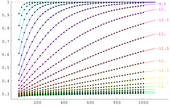
Figure 2: This plot describes the numerical calculation of the $\gamma_{1,3}$ normalization. The horizontal axis is the size of the matrix used and the vertical axis is the normalization. The different graphs are for different values of ${\epsilon}$ between $2^{-6}$ and $2^{-16}$, where some of the intermediate values are labeled. The dots are the calculated values and the lines are just an interpolation we used to guide the eye. For “large” values $({\epsilon}=2^{-6}\sim 0.016)$ the results converge to 1 very rapidly. For extremely small values of ${\epsilon}$ we will have to work with larger and large matrices, but the pattern is clear – eventually the result converges to unity. Interestingly, for ${\epsilon}=0$, even if we take infinite matrices the result will not converge to 1, but to 0.29.

Figure 3: The left plot describes the normalization of the exponential term. The $x$-axis is the $\log$ of the regularization parameter such that ${\epsilon}=0.5^{x}$. The $y$-axis is the argument of the exponent. Therefore, the apparent linear behaviour corresponds to a $\log{\epsilon}$ dependence of the normalization. After ignoring edge points, a linear fit gives $y=-1.29-1.51\log{\epsilon}$. The result from continuous basis calculations is that the coefficient of $\log{\epsilon}$ is $-3/2$. The deviation of the data points from the fit for small $x$ (large ${\epsilon}$) is a result of ignoring ${\cal O}({\epsilon})$ corrections. The deviation of the data points for large $x$ is due to the fact that we are using finite size matrices (1000 by 1000). Up to a total sign the results for the determinant term (right plot) are the same up to the prescribed accuracy. The only qualitative difference is that the deviation for large $x$ starts a bit earlier for the determinant term. This difference is the source of the anomaly seen in the oscillator level truncation.

Another interesting case is the sliver normalization $\left<\infty\vphantom{\infty}\right|\left.\!\vphantom{\infty}{\infty}\right>$. It is of interest because of the extensive use of the sliver state in the literature and because the sliver seems more singular than most other wedge states [38, 45, 46]. We did not try to optimize the numeric calculation and therefore it was limited to 30 by 30 matrices. Still this was enough to demonstrate that the normalization is unity for $s\lesssim 0.9$.

We also computed the overlap of two identity states. This calculation is much more singular since the surface state touches the coordinate patch not only at the mid-point, but also at the entire boundary. Truncating the matrix of the squeezed state also does not help since it gives singular results for every matrix size. Still, using our regularization we can get exact analytical results. For $D$ scalar fields we get

$$\log\det(1-C^{s}C^{s})^{-D/2}=-\frac{D}{2}\operatorname{tr}\log(1-C^{s}C^{s})=-\frac{D}{2}\sum_{n=1}^{\infty}\log(1-s^{4n})\,.$$ (106)

Showing that this expression has radius of convergence of unity proves that our regularization gives a well defined value to the $\left<1\vphantom{1}\right|\left.\!\vphantom{1}{1}\right>$ overlap. We used the scalar field for the calculation, but since the regularization of the scalar field is equivalent to regularizing the Virasoro operators, the above expression is universal after replacing the number of scalar fields $D$ with their central charge $c$.

We are therefore guaranteed to get $\left<1\vphantom{1}\right|\left.\!\vphantom{1}{1}\right>=1$ for a system with central charge 0. We still calculated this explicitly for the system of 26 scalar fields and bosonized ghost. This demonstrates that the regularization works in a highly non trivial way. The expression for the log of the normalization is

$$f(x)\equiv\sum_{n=1}^{\infty}\bigg{(}-\frac{27}{2}\log(1-x^{n})+\frac{9}{2n}\frac{x^{n}}{1-x^{2n}}\Big{(}\big{(}2(-1)^{n}-1\big{)}-\frac{1}{2}x^{n}-\frac{1}{2}\big{(}(-1)^{n}-2\big{)}^{2}x^{n}\Big{)}\bigg{)},$$ (107)

where we define $x\equiv s^{4}$. To evaluate the expression we expand $(1-x^{2n})^{-1}$ in its Taylor series as $\sum_{m=1}^{\infty}x^{2n(m-1)}$. We now have a double sum term which we sum over $n$. Renaming $m\rightarrow n$ we get

$$f(x)=\frac{9}{2}\log\prod_{n=1}^{\infty}\left(\frac{\left(1+x^{n}\right)^{3}\left(1-x^{2n-1}\right)}{\left(1+x^{2n}\right)^{2}\left(1+x^{2n-1}\right)^{2}}\right)=\frac{9}{2}\log\prod_{n=1}^{\infty}(1+x^{n})(1-x^{2n-1})\,.$$ (108)

To see that this expression vanishes we use the identity $(1+x^{2n-1})(1-x^{2n-1})=1-x^{2(2n-1)}$. This leaves us with only even powers of $x$ and gives the relation $f(x)=f(x^{2})$, which means that $f(x)$ is a constant and this constant is obviously zero at $x=0$.

5 Conclusions

In this paper we regularized the string field states by a conformal transformation that shrinks them. An important feature of this regularization is that it is independent of the choice of CFT. Level truncation regularization also shares this feature. The added value of our regularization is analyticity with respect to the shrink parameter $s$. This allows us to study singularities that level truncation cannot see, as was demonstrated with the butterfly state.

Our strategy is to turn on the regulator. Then we can consider each sector of the CFT separately. Without the regulator the calculations in each sector would diverge because of the non-zero central charge. These are the infinities that we regularize. After adding up the results from the different sectors, the regularization is removed giving a consistent result.

Moreover, calculations in our regularization can be much simpler and analytic calculations can be taken much further. Specifically, we can apply our regularization to the continuous basis. All previous calculations in the continuous basis used oscillator level truncation, which is not universal, giving wrong results.

In the continuous basis we managed to calculate the normalization of the commutation relation of Schnabl’s operators and to check, to some extent, the descent relations of the vertices. It would be interesting to try and make an analytical calculation for all the descent relations. We did do some numerical calculations. Since it is impossible to use infinite matrices, the calculation is again CFT dependent. Still, we could take matrices up to 1000 by 1000 in size, which can be considered infinite for $s\lesssim 0.99$. Interestingly, for the most singular calculation, the calculation of the normalization of the identity state, we did manage to perform a fully analytic calculation.

For all singular calculations $s$ has radius of convergence of unity. One could ask what happens at $s=1$. It seems that there could be a phase transition at this point, which adds non trivial constants to the descent relations. In [32] it was suggested that indeed such constants exist and that they can be explained by partition function calculations, yet no one has performed these calculations. In our regularization, this question is irrelevant, since we avoid the need to deal with surfaces with conical singularities. All calculations are consistent in the limit $s\rightarrow 1$, so we can define the value at $s=1$ to be the value of this limit.

Our regularization works for states and vertices. Other string field theory calculations would also require the use of the propagator. There does not appear to be a straightforward generalization of our regularization to the propagator operator. We can hope that either such regularization will not be needed, or that the intuitive geometric picture of our regularization would allow for a simple generalization of our work to this case.

We could also think of generalizing our regularization by replacing $s^{L_{0}}$ with other universal expressions. One asked-for option is to use $s^{{\cal L}_{0}}$ as the regulator. With this choice the calculation of descent relations is much simpler. However, one can easily check that the singularity in the descent relations is not removed. So this operator cannot be used for regularization. This gives us some intuitive understanding about the source of the divergence. The conformal map related to $s^{{\cal L}_{0}}$ shrinks the coordinate patch everywhere except at the mid-point, demonstrating that the mid-point is “the source of all evil”.

Finally, we note that our work is relevant also to other, non-polynomial string field theories. There has been recently an advance in the field, with the definition of the heterotic string field theory [47, 48] and the new results from closed string field theory [49, 50]. These theories are usually dealt with using universal expressions. However, if one would attempt an oscillator approach, then relative normalization coefficients would be even more important than in the case of the cubic theory, where non-trivial factors can in principal be absorbed into the string field.

References

- [1] E. S. Fradkin and A. A. Tseytlin, Nonlinear electrodynamics from quantized strings, Phys. Lett. B163 (1985) 123.
- [2] R. R. Metsaev, M. A. Rakhmanov, and A. A. Tseytlin, The Born-Infeld action as the effective action in the open superstring theory, Phys. Lett. B193 (1987) 207.
- [3] E. Witten, Noncommutative geometry and string field theory, Nucl. Phys. B268 (1986) 253.
- [4] D. J. Gross and A. Jevicki, Operator formulation of interacting string field theory, Nucl. Phys. B283 (1987) 1.
- [5] D. J. Gross and A. Jevicki, Operator formulation of interacting string field theory. 2, Nucl. Phys. B287 (1987) 225.
- [6] S. Samuel, The physical and ghost vertices in Witten’s string field theory, Phys. Lett. B181 (1986) 255.
- [7] N. Ohta, Covariant interacting string field theory in the Fock space representation, Phys. Rev. D34 (1986) 3785–3793.
- [8] E. Cremmer, A. Schwimmer, and C. B. Thorn, The vertex function in Witten’s formulation of string field theory, Phys. Lett. B179 (1986) 57.
- [9] A. LeClair, M. E. Peskin, and C. R. Preitschopf, String field theory on the conformal plane. 1. kinematical principles, Nucl. Phys. B317 (1989) 411.
- [10] A. LeClair, M. E. Peskin, and C. R. Preitschopf, String field theory on the conformal plane. 2. generalized gluing, Nucl. Phys. B317 (1989) 464.
- [11] I. Bars, Map of Witten’s * to Moyal’s *, Phys. Lett. B517 (2001) 436–444, [hep-th/0106157].
- [12] I. Bars and Y. Matsuo, Computing in string field theory using the Moyal star product, Phys. Rev. D66 (2002) 066003, [hep-th/0204260].
- [13] I. Bars, MSFT: Moyal star formulation of string field theory, hep-th/0211238.
- [14] M. Schnabl, Analytic solution for tachyon condensation in open string field theory, Adv. Theor. Math. Phys. 10 (2006) 433–501, [hep-th/0511286].
- [15] A. Sen, Descent relations among bosonic D-branes, Int. J. Mod. Phys. A14 (1999) 4061–4078, [hep-th/9902105].
- [16] A. Sen, Universality of the tachyon potential, JHEP 12 (1999) 027, [hep-th/9911116].
- [17] Y. Okawa, Comments on Schnabl’s analytic solution for tachyon condensation in Witten’s open string field theory, JHEP 04 (2006) 055, [hep-th/0603159].
- [18] E. Fuchs and M. Kroyter, On the validity of the solution of string field theory, JHEP 05 (2006) 006, [hep-th/0603195].
- [19] I. Ellwood and M. Schnabl, Proof of vanishing cohomology at the tachyon vacuum, hep-th/0606142.
- [20] D. Gaiotto, L. Rastelli, A. Sen, and B. Zwiebach, Patterns in open string field theory solutions, JHEP 03 (2002) 003, [hep-th/0201159].
- [21] L. Rastelli and B. Zwiebach, Solving open string field theory with special projectors, hep-th/0606131.
- [22] E. Fuchs and M. Kroyter, Schnabl’s operator in the continuous basis, JHEP 10 (2006) 067, [hep-th/0605254].
- [23] H. Fuji, S. Nakayama, and H. Suzuki, Open string amplitudes in various gauges, hep-th/0609047.
- [24] L. Rastelli and B. Zwiebach, Tachyon potentials, star products and universality, JHEP 09 (2001) 038, [hep-th/0006240].
- [25] K. Furuuchi and K. Okuyama, Comma vertex and string field algebra, JHEP 09 (2001) 035, [hep-th/0107101].
- [26] L. Rastelli, A. Sen, and B. Zwiebach, Boundary CFT construction of D-branes in vacuum string field theory, JHEP 11 (2001) 045, [hep-th/0105168].
- [27] M. Schnabl, Wedge states in string field theory, JHEP 01 (2003) 004, [hep-th/0201095].
- [28] D. M. Belov and A. Konechny, On continuous Moyal product structure in string field theory, JHEP 10 (2002) 049, [hep-th/0207174].
- [29] E. Fuchs, M. Kroyter, and A. Marcus, Virasoro operators in the continuous basis of string field theory, JHEP 11 (2002) 046, [hep-th/0210155].
- [30] D. M. Belov and A. Konechny, On spectral density of Neumann matrices, Phys. Lett. B558 (2003) 111–118, [hep-th/0210169].
- [31] E. Fuchs, M. Kroyter, and A. Marcus, Continuous half-string representation of string field theory, JHEP 11 (2003) 039, [hep-th/0307148].
- [32] D. M. Belov, Witten’s ghost vertex made simple (bc and bosonized ghosts), Phys. Rev. D69 (2004) 126001, [hep-th/0308147].
- [33] M. R. Douglas, H. Liu, G. Moore, and B. Zwiebach, Open string star as a continuous Moyal product, JHEP 04 (2002) 022, [hep-th/0202087].
- [34] D. M. Belov, Representation of small conformal algebra in kappa-basis, hep-th/0210199.
- [35] E. Fuchs and M. Kroyter, Normalization anomalies in level truncation calculations, JHEP 12 (2005) 031, [hep-th/0508010].
- [36] I. Y. Aref’eva, R. Gorbachev, P. B. Medvedev, and D. V. Rychkov, Descent relations and oscillator level truncation method, hep-th/0606070.
- [37] V. A. Kostelecky and S. Samuel, On a nonperturbative vacuum for the open bosonic string, Nucl. Phys. B336 (1990) 263.
- [38] L. Rastelli, A. Sen, and B. Zwiebach, Star algebra spectroscopy, JHEP 03 (2002) 029, [hep-th/0111281].
- [39] W. Taylor, Perturbative diagrams in string field theory, hep-th/0207132.
- [40] W. Taylor, Perturbative computations in string field theory, hep-th/0404102.
- [41] K. Okuyama, Ratio of tensions from vacuum string field theory, JHEP 03 (2002) 050, [hep-th/0201136].
- [42] S. Uhlmann, A note on kappa-diagonal surface states, JHEP 11 (2004) 003, [hep-th/0408245].
- [43] E. Fuchs and M. Kroyter, On surface states and star-subalgebras in string field theory, JHEP 10 (2004) 004, [hep-th/0409020].
- [44] V. A. Kostelecky and R. Potting, Analytical construction of a nonperturbative vacuum for the open bosonic string, Phys. Rev. D63 (2001) 046007, [hep-th/0008252].
- [45] G. Moore and W. Taylor, The singular geometry of the sliver, JHEP 01 (2002) 004, [hep-th/0111069].
- [46] D. Gaiotto, L. Rastelli, A. Sen, and B. Zwiebach, Star algebra projectors, JHEP 04 (2002) 060, [hep-th/0202151].
- [47] Y. Okawa and B. Zwiebach, Heterotic string field theory, JHEP 07 (2004) 042, [hep-th/0406212].
- [48] N. Berkovits, Y. Okawa, and B. Zwiebach, WZW-like action for heterotic string field theory, JHEP 11 (2004) 038, [hep-th/0409018].
- [49] H. Yang and B. Zwiebach, A closed string tachyon vacuum?, JHEP 09 (2005) 054, [hep-th/0506077].
- [50] N. Moeller and H. Yang, The nonperturbative closed string tachyon vacuum to high level, hep-th/0609208.