Quantum Field Theory in de Sitter space : A survey of recent approaches.

Abstract

We present a survey of rigourous quantization results obtained in recent works on quantum free fields in de Sitter space. For the “massive” cases which are associated to principal series representations of the de Sitter group $SO_{0}(1,4)$, the construction is based on analyticity requirements on the Wightman two-point function. For the “massless” cases (e.g. minimally coupled or conformal), associated to the discrete series, the quantization schemes are of the Gupta-Bleuler-Krein type.

1 Introduction

It is valuable to start out this review of recent results on de Sitter quantum field theory by quoting a sentence from the well-known Wald’s monograph [37] on QFT in curved space-time :

It is worth noting that most of the available treatments of quantum field theory in curved spacetime either are oriented strongly toward mathematical issues (and deal, e.g., with $C^{\ast}$-algebras, KMS states, etc.) or are oriented toward a concrete physical problem (and deal, e.g., with particular mode function expansions of a quantum field in a certain spacetime).

De Sitter and Anti de Sitter space-times play a fundamental role in cosmology, since they are, with Minkowski spacetime, the only maximally symmetric space-time solutions in general relativity. Their respective invariance (in the relativity or kinematical sense) groups are the ten-parameters de Sitter $SO_{\scriptsize 0}(1,4)$ and anti de Sitter $SO_{\scriptsize 0}(2,3)$ groups. Both may be seen as deformations of the proper orthochronous Poincaré group $\mathbb{R}^{1,3}\rtimes\,S0_{\scriptsize 0}(1,3)$, the kinematical group of Minkowski spacetime.

The de Sitter [resp. anti-de Sitter] space-times are solutions to the vacuum Einstein’s equations with positive [resp. negative] cosmological constant $\Lambda$. This constant is linked to the (constant) Ricci curvature $4\Lambda$ of these space-times. The corresponding fundamental length is given by $H^{-1}:=\sqrt{3/(c\Lambda)}$

Serious reasons back up any interest in studying Physics in such constant curvature spacetimes with maximal symmetry. The first one is the simplicity of their geometry, which makes consider them as an excellent laboratory model in view of studying Physics in more elaborate universes, more precisely with the purpose to set up a quantum field theory as much rigorous as possible [22, 2, 10, 37].

Higher dimensional Anti de Sitter spaces have becoming in the last years very popular because of their regularizing geometries. For instance they play an important role in some versions of string or branes theories, and constitute presently the only cosmological example of the holographic conjecture.

Recent calculations [25] suggested that the de Sitter solution may play an universal role as an “osculating” manifold for space-time.

Since the beginning of the eighties, the de Sitter space has been playing a much popular role in inflationary cosmological scenarii [24], where it is assumed that the cosmic dynamics was dominated by a term acting like a cosmoloical constant. More recently , observations on far high redshift supernovae [29], on galaxy clusters [30], and on cosmic microwave background radiation [6] suggested an accelerating universe. Again, this can be explained only with such a term.

On a fundamental level, matter and energy are of quantum nature. But the usual quantum field theory is designed in Minkowski spacetime. Many theoretical and observational arguments plead in favour of setting up a rigorous quantum field theory in de Sitter, and compare with our familiar minkowskian quantum field theory. As a matter of fact, the symmetry properties of the dS solutions may allow the construction of such a theory.

Also, the study of de Sitter space-time offers a specific interest because of the regularization opportunity afforded by the curvature parameter as a “natural” cutoff for infrared or other divergences.

On the other hand, as it will appear here, some of our most familiar concepts like time, energy, momentum, etc, disappear. They really need a new conceptual approach in de Sitterian relativity. However, it should be stressed that the current estimate on the cosmological constant does not allow any palpable experimental effect on the level of high energy physics experiments, unless, as is explained in [18], we deal with theories involving assumptions of infinitesimal masses like photon or graviton masses. We will tell more about this throughout the paper.

To summarize, the interest of setting up a QFT in de Sitter spacetime stems from

• dS is maximally symmetric

• Its symmetry is a one-parameter (curvature) deformation of minkowskian symmetry

• It is so an excellent laboratory for both, mathematical or concrete, approaches to QFT

• As soon as a constant curvature is present (like the currently observed one!), we lose some of our so familiar conservation laws like energy-momentum conservation.

• What is then the physical meaning of a scattering experiment (“space” in dS is like the sphere $S^{3}$, let alone the fact that time is ambiguous)?

• Which relevant “physical” quantities are going to be considered as (asymptotically?, contractively?) experimentally available?

The recent results on de Sitter Quantum Field Theory which we would like to report here can be viewed as a part of this program of understanding physics in the de Sitter universe. Of course, a huge amount of work has been done on de Sitter both on a classical and a quantum level since the Einstein’s cosmological “mistake” and the first geometrical studies by de Sitter himself. For reasons that will become clear below, present results are divided into two categories. The first category concerns the “massive” fields, so called for having Poincaré massive limits at null curvature. They have been developped in [4, 5, 3, 36, 21, 1, 12], and they are essentially characterised by analyticity properties of their Wightman two-point functions. The other category, developped in [7, 20, 32, 13, 14], deals with massless fields and other relevant fields, which require non standard quantization procedures. Both categories have a strong group theoretical flavor since they share, as a common obvious constraint, de Sitter covariance.

After describing the de Sitter geometry and kinematics (space and group) in Section 2, we give in Section 3 the complete list of unitary irreducible representations of the de Sitter group and their possible contractive relations with the Wigner Poincaré representations. Then we review in Sections 4 and 5 the main points of de Sitter QFT, pertaining to axiomatics as well as to technicality and problematic. Section 4 is devoted to de Sitter QFT for principal series (or “massive”) fields based on the Wightman two-point function. We explain in Section 5, through the example of the “massless” minimally coupled quantum field, how a new quantization, based on a Krein space of solutions of the de Sitter wave equation, allows to successfully deal with other fields like those pertaining to the discrete series.

2 De Sitter geometry and kinematics

2.1 The hyperboloid

The de Sitter metric is the unique solution of the cosmological vacuum Einstein’s equation with positive cosmological constant $\Lambda=3~{}H^{2}$ (in units $c=1$).

$$R_{\mu\nu}-\frac{1}{2}Rg_{\mu\nu}+\Lambda g_{\mu\nu}=0,$$ (1)

$$R=R_{\mu\nu}g^{\mu\nu}=4\Lambda\equiv 12H^{2}.$$

The corresponding de Sitter space is conveniently seen as an one-sheeted hyperboloid (Fig 1) embedded in a five-dimensional Minkowski space (the bulk):

$$M_{H}\equiv\{x\in{\rm I\!R}^{5};~{}x^{2}=\eta_{\alpha\beta}~{}x^{\alpha}x^{\beta}=-H^{-2}\},\;\;\alpha,\beta=0,1,2,3,4,$$ (2)

where $\eta_{\alpha\beta}=$diag$(1,-1,-1,-1,-1)$.

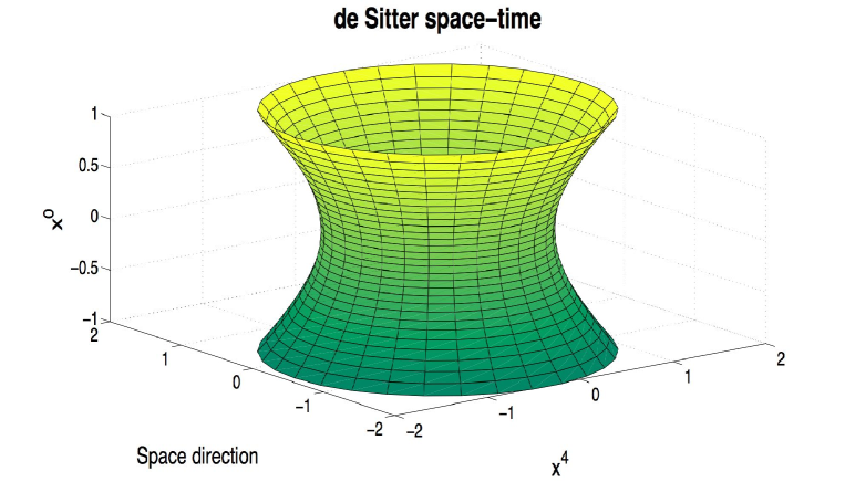
Figure 1: de Sitter space-time as a hyperboloid embedded in a five-dimensional Minkowski space

We can, for instance, adopt the following system of global coordinates :

$$x :=(x^{0},\vec{x},x^{4})$$

$$x^{0} =H^{-1}~{}\sinh(H\tau)$$

$$\vec{x} =(x^{1},x^{2},x^{3})=H^{-1}~{}\cosh(H\tau)~{}\sin(H\rho)~{}\vec{n}$$

$$x^{4} =H^{-1}~{}\cosh(H\tau)~{}\cos(H\rho)$$ (3)

where $\vec{n}$ is a spatial direction, i.e., a spatial unit vector of ${\rm I\!R}^{3}$, and $R=H^{-1}$ for a point of the hyperboloid.

There is a global causal ordering on the de Sitter manifold which is induced from that of the ambient spacetime ${\mathbb{R}}^{5}$: given two events $x,y\in M_{H}$, one says that $x\geq y$ iff $x-y\in\overline{V^{+}}$, where $\overline{V^{+}}=\{x\in{\mathbb{R}}^{5}:x\cdot x\geq 0,\ {\rm sgn}\,x^{0}={+}\}$ is the future cone in ${{\rm I\!R}}^{5}$.

The closed causal future (resp. past) cone of a given point $x$ in $X$ is therefore the set $\{y\in M_{H}:y\geq x\}$ (resp. $\{y\in M_{H}:y\leq x\}$). Two events $x,y\in M_{H}$ are said in “acausal relation” or “spacelike separated” if they belong to the intersection of the complements of such sets, i.e. if $(x-y)^{2}=-2(H^{-2}+x\cdot y)<0$.

2.2 The de Sitter group

The de Sitter relativity group is $G=SO_{0}(1,4)$, i.e. the component connected to the identity of the ten-dimensional pseudo-orthogonal group $SO(1,4)$. A familiar realization of the Lie algebra is that one generated by the ten Killing vectors

$$K_{\alpha\beta}=x_{\alpha}\partial_{\beta}-x_{\beta}\partial_{\alpha}.$$ (4)

It is worthy to notice that there is no globally time-like Killing vector in de Sitter, the adjective time-like (resp. space-like) referring to the Lorentzian four-dimensional metric induced by that of the bulk.

The universal covering of the de Sitter group is the symplectic $Sp(2,2)$ group, which is needed when dealing with half-integer spins. It is suitably described as a subgroup of the group of $2\times 2$ matrices with quaternionic coefficients:

$$Sp(2,2)=\left\{g=\left(\begin{array}[]{cc}a&b\\ c&d\\ \end{array}\right);\ a,b,c,d\in\mathbb{H},\ {\det}_{\scriptsize 4\times 4}g=1,\ g^{\dagger}\gamma^{0}g=\gamma^{0}\right\}.$$ (5)

We recall that the group of quaternions $\mathbb{H}\simeq\mathbb{R}_{+}\times SU(2)$. We write $(1\equiv e_{4},,e_{i}$ ($\simeq(-1)^{i+1}\sigma_{i})$ in $2\times 2$-matrix notations) the canonical basis for $\mathbb{H}\simeq\mathbb{R}^{4}$, with $i=1,2,3$: any quaternion will be written $q=(q^{4},\vec{q})$ (resp. $q^{a}~{}e_{a},~{}a=1,2,3,4$) in scalar-vector notations (resp. in euclidean metric notation). We also recall that the multiplication law is $qq^{\prime}=(q^{4}{q^{\prime}}^{4}-\vec{q}\cdot\vec{q^{\prime}},{q^{\prime}}^{4}\vec{q}+{q}^{4}\vec{q^{\prime}}+\vec{q}\times\vec{q^{\prime}})$, the (quaternionic) conjugate of $q=(q^{4},\vec{q})$ is $\bar{q}=(q^{4},-\vec{q})$, the squared norm is $\|q\|^{2}=q\bar{q}$, and the inverse of a nonzero quaternion is $q^{-1}=\bar{q}/\|q\|^{2}$.

We have written $g^{\dagger}=\bar{g}^{\scriptsize t}$ for the quaternionic conjugate and transpose of the matrix $g$. The matrix

$$\gamma^{0}=\left(\begin{array}[]{cc}1&0\\ 0&-1\\ \end{array}\right)$$ (6)

is part of the Clifford algebra $\gamma^{\alpha}\gamma^{\beta}+\gamma^{\beta}\gamma^{\alpha}=2\eta^{\alpha\beta}\mathbb{I}$, the four other matrices having the following form in this quaternionic representation:

$$\gamma^{4}=\left(\begin{array}[]{cc}0&1\\ -1&0\\ \end{array}\right),\ \gamma^{k}=\left(\begin{array}[]{cc}0&e_{k}\\ e_{k}&0\\ \end{array}\right),\ k=1,2,3.$$ (7)

These matrices allow the following correspondence between points of the hyperboloid $M_{H}$ and $2\times 2$ quaternionic matrices of the form below:

$$M_{H}\ni x\longrightarrow\not\!x\equiv x^{\alpha}\gamma_{\alpha}=\left(\begin{array}[]{cc}x^{0}&-{\cal P}\\ \overline{\cal P}&-x^{0}\\ \end{array}\right),$$ (8)

where ${\cal P}\equiv(x^{4},\vec{x})\in\mathbb{H}$. Note that we have

$$x\cdot x=\not\!x^{{\dagger}}\gamma^{0}\not\!x\gamma^{0},~{}~{}x^{0}=\frac{1}{4}\mbox{tr}\gamma^{0}\not\!x.$$ (9)

The de Sitter action on $M_{H}$ is then simply given by

$$Sp(2,2)\ni g:\ \not\!x\longrightarrow g\not\!xg^{-1}=\not\!x^{\prime},$$ (10)

and this precisely realizes the isomorphism $SO_{\scriptsize 0}(1,4)\longrightarrow Sp(2,2)/\mathbb{Z}_{2}$ through

$$SO_{\scriptsize 0}(1,4)\ni\Lambda(g):\ x\longrightarrow\Lambda(g)x=x^{\prime},\ \Lambda^{\alpha}_{\beta}=\frac{1}{4}\mbox{tr}(\gamma^{\alpha}g\gamma_{\beta}g^{-1}).$$ (11)

Another way to understand this group action on de Sitter is to resort to a specific (nonglobal) factorization of the group one can call space-time factorization and which is based on the group involution $g\longrightarrow\vartheta(g)=\gamma^{0}\gamma^{4}g^{\dagger}\gamma^{0}\gamma^{4}$:

$$g=jl,\ j=\left(\begin{array}[]{cc}\eta&0\\ 0&\bar{\eta}\\ \end{array}\right)\left(\begin{array}[]{cc}\cosh{\frac{\psi}{2}}&\sinh{\frac{\psi}{2}}\\ \sinh{\frac{\psi}{2}}&\cosh{\frac{\psi}{2}}\\ \end{array}\right),\ l=\left(\begin{array}[]{cc}\zeta&0\\ 0&\zeta\\ \end{array}\right)\left(\begin{array}[]{cc}\cosh{\frac{\varphi}{2}}&\hat{u}\sinh{\frac{\varphi}{2}}\\ -\hat{u}\sinh{\frac{\varphi}{2}}&\cosh{\frac{\varphi}{2}}\\ \end{array}\right),$$ (12)

where $\psi,\varphi\in\mathbb{R},\ \zeta,\eta,\hat{u}=-\bar{\hat{u}}$ (“pure” vector quaternion) $\in SU(2)$. The factor $l$ is element of the (Lorentz) subgroup $L=\{l\in Sp(2,2);\ l\vartheta(l)=\mathbb{I}\}\simeq SL(2,\mathbb{C})$ and the parameters $\zeta,\hat{u},\varphi$ have the meaning of space rotation, boost velocity direction and rapidity respectively. The factor $j$ is a kind of “space-time” square root since we have

$$j\vartheta(j)=\left(\begin{array}[]{cc}\eta^{2}\cosh{\psi}&\sinh{\psi}\\ \sinh{\psi}&\overline{\eta^{2}}\cosh{\psi}\\ \end{array}\right)\equiv\left(\begin{array}[]{cc}x^{0}&-{\cal P}\\ \overline{\cal P}&-x^{0}\\ \end{array}\right)\left(\begin{array}[]{cc}0&1\\ -1&0\\ \end{array}\right)=\not\!x\gamma^{4},$$ (13)

where the equivalence holds modulo a determinant factor. We thus see that the group action (10) is directly issued from the left action of the group on the coset $G/L$ through $j\longrightarrow gj=j^{\prime}l^{\prime}$. The Lorentz subgroup L is actually the stabilizer of $H^{-1}\gamma^{0}\gamma^{4}$. The latter corresponds to the point $O_{H}=(0,0,0,0,H^{-1})$ chosen as origin of the de Sitter universe, and $j$ maps this origin to the point $(x^{0},{\cal P})$ in the notations (8). Note that the set $\{\psi,\eta^{2}\}$ in (13) provides, through $x^{0}=\sinh{\psi},{\cal P}=\eta^{2}\cosh{\psi}$, the system of global coordinates (2.1) for $M_{H}$.

De Sitterian classical mechanics is understood along the traditional phase space approach. By phase space for an elementary system in de Sitter universe, we mean an orbit of the coadjoint representation of the group. We know that such an orbit is a symplectic manifold, and, as an homogeneous space, is homeomorphic to an even-dimensional group coset $Sp(2,2)/H_{S}$, where $H_{S}$ is the stabilizer subgroup of some orbit point. As a matter of fact, a scalar “massive” elementary system in de Sitter corresponds to the coset $Sp(2,2)/H_{S}$ where the subgroup $H_{S}$ is made up with “space” rotations and “time” translations in agreement with the space-time factorization (12) of $Sp(2,2)$:

$$H_{S}=\left\{g=\left(\begin{array}[]{cc}\zeta&0\\ 0&\zeta\\ \end{array}\right)\left(\begin{array}[]{cc}\cosh{\frac{\psi}{2}}&\sinh{\frac{\psi}{2}}\\ \sinh{\frac{\psi}{2}}&\cosh{\frac{\psi}{2}}\\ \end{array}\right),\ \zeta\in SU(2),\ \psi\in\mathbb{R}\right\}.$$ (14)

3 De Sitter UIR and their physical interpretation

Specific quantization procedures [33, 23, 19] applied to the above classical phase spaces leads to their quantum counterparts, namely the quantum elementary systems associated in a biunivocal way to the the UIR’s of the de Sitter group $Sp(2,2)$. Let us give a complete classification of the latter, following the works by Dixmier [9] and Takahashi [35]. We recall that the ten Killing vectors (4) can be represented as (essentially) self-adjoint operators in Hilbert space of (spinor-)tensor valued functions on $M_{H}$, square integrable with respect to some invariant inner product, more precisely of the Klein-Gordon type. These operators take the form

$$K_{\alpha\beta}\longrightarrow L_{\alpha\beta}=M_{\alpha\beta}+S_{\alpha\beta},$$ (15)

where the orbital part is $M_{\alpha\beta}=-i(x_{\alpha}\partial_{\beta}-x_{\beta}\partial_{\alpha})$ and the spinorial part $S_{\alpha\beta}$ acts on the indices of functions in a certain permutational way. There are two Casimir operators, the eigenvalues of which determine completely the UIR’s. They read:

$$Q^{(1)}=-\frac{1}{2}L_{\alpha\beta}L^{\alpha\beta},$$ (16)

with eigenvalues $-p(p+1)-(q+1)(q-2)$ and

$$Q^{(2)}=-W_{\alpha}W^{\alpha},\ W_{\alpha}=-\frac{1}{8}\epsilon_{\alpha\beta\gamma\delta\eta}L^{\beta\gamma}L^{\delta\eta},$$ (17)

with eigenvalues $-p(p+1)q(q-1)$. Therefore, one must distinguish between

• The discrete series $\Pi^{\pm}_{p,q}$,
  defined by $p$ and $q$ having integer or half-integer values, $p\geq q$. Note that $q$ may have a spin meaning.

  Here, we must again distinguish between

  • The scalar case $\Pi_{p,0}$, $p=1,2,\cdots$; hereafter we refer to it as Dsc;

  • The spinorial case $\Pi^{\pm}_{p,q}$, $q>0$, $p=\frac{1}{2},1,\frac{3}{2},2,\cdots$, $q=p,p-1,\cdots,1$ or $\frac{1}{2}$:Dsp

• The principal and complementary series $\Upsilon_{p,\sigma}$,
  where $p$ has a spin meaning. We put $\sigma=q~{}(1-q)$ which gives $q=\frac{1}{2}\left(1\pm\sqrt{1-4\sigma^{2}}\right)$.

  Like in the above, one distinguishes between

  • The scalar case $\Upsilon_{0,\sigma}$, where

    • $-2<\sigma<\frac{1}{4}$ for the complementary series: Cscm, Csc0 for $\sigma=0$;

    • $\frac{1}{4}\leq\sigma$ for the principal series: Pscm.

  • The spinorial case $\Upsilon_{p,\sigma}$, $p>0$, where

    • $0<\sigma<\frac{1}{4}$, $p=1,2,\cdots$, for the complementary series: Cspm,

    • $\frac{1}{4}\leq\sigma$, $p=1,2,\cdots$, for the integer spin principal series: Pspm,

    • $\frac{1}{4}<\sigma$, $p=\frac{1}{2},\frac{3}{2},\frac{5}{2}\cdots$, for the half-integer spin principal series: Pspm.

3.1 Contraction limits

An important question to be addressed concerns the interpretation of these UIR’s (or quantum de Sitter elementary systems) from a Minkowskian point of view. We mean by this the study of the contraction limit $H\to 0$ of these representations, which is the quantum counterpart of the following geometrical and group contractions

• $\lim_{H\to 0}M_{H}=M_{0}$, the Minkowski spacetime tangent to $M_{H}$ at, say, the de Sitter origin point $O_{H}$,

• $\lim_{H\to 0}Sp(2,2)={\cal P}^{\uparrow}_{+}(1,3)=M_{0}\rtimes SL(2,\mathbb{C})$, the Poincaré group.

As a matter of fact, the ten de Sitter Killing vectors (4) contract to their Poincaré counterparts $K_{\mu\nu}$, $\Pi_{\mu}$, $\mu=0,1,2,3$, after rescaling the four $K_{4\mu}\longrightarrow\Pi_{\mu}=HK_{4\mu}$.

Now, we have to distinguish between the Poincaré massive and massless cases. We shall denote by ${\cal P}^{\stackrel{{\scriptstyle>}}{{<}}}(m,s)$ the positive (resp. negative) energy Wigner UIR’s of the Poincaré group with mass $m$ and spin $s$. For interesting discussion and precision on this confusing notion of mass in “desitterian Physics”, we will give below details on the work by Garidi [16]. We shall make use of similar notation ${\cal P}^{\stackrel{{\scriptstyle>}}{{<}}}(0,s)$ for the Poincaré massless case where $s$ reads for helicity. In the latter case, conformal invariance leads us to deal also with the discrete series representations (and their lower limits) of the (universal covering of the) conformal group or its double covering $SO_{0}(2,4)$ or its fourth covering $SU(2,2)$. These UIR’s are denoted in the sequel by ${\cal C}^{\stackrel{{\scriptstyle>}}{{<}}}(E_{0},j_{1},j_{2})$, where $(j_{1},j_{2})\in\mathbb{N}/2\times\mathbb{N}/2$ labels the UIR’s of $SU(2)\times SU(2)$ and $E_{0}$ stems for the positive (resp. negative) conformal energy. The de Sitter contraction limits can be summarized in the following diagrams.

Massive case

Solely the principal series representations Pscm and Pspm are involved here (from where comes the name of de Sitter “massive representations”). Introducing the parameter $\nu$ through $\sigma=\nu^{2}+1/4$, and the Poincaré mass $m=\nu H$, we have [27, 15]

$${\Upsilon}_{s,\sigma}\longrightarrow_{H\to 0,\nu\to\infty}{c_{>}\cal P}^{>}(m,s)\oplus c_{<}{\cal P}^{<}(m,s),$$ (18)

where one of the “coefficients” among $c_{<},c_{>}$ can be fixed to 1 whilst the other one will vanishes. Note here the evidence of the energy ambiguity in de Sitter relativity, exemplified by the possible breaking of dS irreducibility into a direct sum of two Poincaré UIR’s with positive and negative energy respectively. This phenomenon is linked to the existence in the de Sitter group of a specific discrete symmetry, precisely $\gamma_{0}\in Sp(2,2)$, which sends any point $(x^{0},{\cal P})\in M_{H}$ (with the notations of (2.7)) into its mirror image $(x^{0},-{\cal P})\in M_{H}$ with respect to the $x^{0}$-axis. Under such a symmetry the four generators $L_{a0}$, $a=1,2,3,4$, (and particularly $L_{40}$ which contracts to energy operator!) transform into their respective opposite $-L_{a0}$, whereas the six $L_{ab}$’s remain unchanged.

Note that the well-known ambiguity concerning the existence of a vacuum (“$\alpha$-vacua”) in de Sitter quantum field theory originates in the above contraction arbitrariness.

In the context of the notion of mass in “desitterian Physics”, the following “mass” formula has been proposed by Garidi [16] in terms of the dS RUI parameters $p$ and $q$:

$$m^{2}_{H}=\langle Q^{(1)}\rangle_{\mathrm{dS}}-\langle Q^{(1)}_{p=q}\rangle_{\mathrm{dS}}=[(p-q)(p+q-1)]\hbar^{2}H^{2}/c^{4}.$$ (19)

This formula is natural in the sense that when the second-order wave equation

$$\left(Q^{(1)}-\langle Q^{(1)}\rangle_{\mathrm{dS}}\right)\varphi=0,$$

obeyed by rank $r$ tensor fields carrying a dS UIR, is written in terms of the Laplace-Beltrami operator $\Box_{H}$ on the dS manifold, one gets (in units $\hbar=1=c$)

$$\left(\Box_{H}+H^{2}r(r+2)+H^{2}\langle Q^{(1)}\rangle_{\mathrm{dS}}\right)\varphi=0.$$ (20)

Moreover, the minimal value assumed by the eigenvalues of the first Casimir in the set of RUI in the discrete series is precisely reached at $p=q$, which corresponds to the “conformal” massless case. The Garidi mass has the advantages to encompass all mass formulas introduced within a de-sitterian context, often in a purely mimetic way in regard with their minkowskian counterparts.

Actually, given a minkowskian mass $m$ and a “universal” length $R=:\sqrt{3/|\Lambda|}=c\,H^{-1}$ (we here restore for a moment all physical units) , nothing prevents us to consider the dS UIR parameter $\nu$ (principal series), specific of a “physics” in constant-curvature space-time, as a meromorphic functions of the dimensionless physical (in the minkowskian sense!) quantity, expressed in terms of various other quantities introduced in this paper,

$$\vartheta\equiv\vartheta_{m}\stackrel{{\scriptstyle\mathrm{def}}}{{=}}\frac{\hbar}{Rmc}=\frac{\hbar\sqrt{|\Lambda}|}{\sqrt{3}mc}=\frac{\hbar\,H}{mc^{2}}.$$ (21)

We give in Table 1 the values assumed by the quantity $\vartheta$ when $m$ is taken as some known masses and $\Lambda$ (or $H_{0}$) is given its present day estimated value. We easily understand from this table that the currently estimated value of the cosmological constant has no practical effect on our familiar massive fermion or boson fields. Contrariwise, adopting the de Sitter point of view appears as inescapable when we deal with infinitely small masses, as is done in standard inflation scenario.

Mass $m$	$\vartheta_{m}\approx$
$m_{\Lambda}/\sqrt{3}\approx 0.293\times 10^{-68}$kg	1
up. lim. photon mass $m_{\gamma}$	$0.29\times 10^{-16}$
up. lim. neutrino mass $m_{\nu}$	$0.165\times 10^{-32}$
electron mass $m_{e}$	$0.3\times 10^{-37}$
proton mass $m_{p}$	$0.17\times 10^{-41}$
$W^{\pm}$ boson mass	$0.2\times 10^{-43}$
Planck mass $M_{Pl}$	$0.135\times 10^{-60}$

Table 1: Estimated values of the dimensionless physical quantity $\vartheta\equiv\vartheta_{m}=:\frac{\hbar\sqrt{|\Lambda}|}{\sqrt{3}mc}=\frac{\hbar\,H}{mc^{2}}\approx 0.293\times 10^{-68}\times m_{\mathrm{kg}}^{-1}$ for some known masses $m$ and the present day estimated value of the Hubble length $c/H_{0}\approx 1.2\times 10^{26}\mathrm{m}$ [26].

Now, we may consider the following Laurent expansions of the principal series dS UIR parameter $\nu$ in a certain neighborhood of $\vartheta=0$:

$$\nu=\nu(\vartheta)=\frac{1}{\vartheta}+e_{0}+e_{1}\vartheta+\cdots e_{n}\vartheta^{n}+\cdots,\ \vartheta\in(0,\vartheta_{1})\ \mbox{convergence interval},$$ (22)

Coefficients $e_{n}$ are pure numbers to be determined. We should be aware that nothing is changed in the contraction formulas from the point of view of a minkowskian observer, except that we allow to consider positive as well as negative values of $\nu$ in a (positive) neighborhood of $\vartheta=0$: multiply this formula by $\vartheta$ and go to the limit $\vartheta\to 0$. We recover asymptotically the relation

$$m=|\nu|\hbar H/c^{2}=|\nu|\frac{\hbar}{c}\sqrt{\frac{|\Lambda|}{3}}.$$ (23)

As a matter of fact, the Garidi mass is perfect example of such an expansion since it can be rewritten as the following expansion in the parameter $\vartheta\in(0,1/|s-1/2|]$:

$$\nu=\sqrt{\frac{1}{\vartheta^{2}}-(s-1/2)^{2}}$$

$$=\frac{1}{\vartheta}-(s-1/2)^{2}\left(\frac{\vartheta}{2}+O(\vartheta^{2})\right),$$ (24)

Note the particular symmetric place occupied by the spin $1/2$ case with regard to the scalar case $s=0$ and the boson case $s=1$. More details concerning this discussion are given in [18].

Massless (conformal) case

Here we must distinguish between the scalar massless case, which involves the unique complementary series UIR $\Upsilon_{0,0}$ to be contractively Poincaré significant, and the spinorial case where are involved all representations $\Pi^{\pm}_{s,s},\ s>0$ lying at the lower limit of the discrete series. The arrows $\hookrightarrow$ below designate unique extension.

• Scalar massless case : Csc0.

  $$\left.\begin{array}[]{ccccccc}&&{\cal C}^{>}(1,0,0)&&{\cal C}^{>}(1,0,0)&\hookleftarrow&{\cal P}^{>}(0,0)\\ \Upsilon_{0,0}&\hookrightarrow&\oplus&\stackrel{{\scriptstyle H=0}}{{\longrightarrow}}&\oplus&&\oplus\\ &&{\cal C}^{<}(-1,0,0)&&{\cal C}^{<}(-1,0,0)&\hookleftarrow&{\cal P}^{<}(0,0),\\ \end{array}\right.$$ (25)

• Spinorial massless case : Dsp0.

  $$\left.\begin{array}[]{ccccccc}&&{\cal C}^{>}(s+1,s,0)&&{\cal C}^{>}(s+1,s,0)&\hookleftarrow&{\cal P}^{>}(0,s)\\ \Pi^{+}_{s,s}&\hookrightarrow&\oplus&\stackrel{{\scriptstyle H=0}}{{\longrightarrow}}&\oplus&&\oplus\\ &&{\cal C}^{<}(-s-1,s,0)&&{\cal C}^{<}(-s-1,s,0)&\hookleftarrow&{\cal P}^{<}(0,s),\\ \end{array}\right.$$ (26)

  $$\left.\begin{array}[]{ccccccc}&&{\cal C}(s+1,0,s)&&{\cal C}^{>}(s+1,0,s)&\hookleftarrow&{\cal P}^{>}(0,-s)\\ \Pi^{-}_{s,s}&\hookrightarrow&\oplus&\stackrel{{\scriptstyle H=0}}{{\longrightarrow}}&\oplus&&\oplus\\ &&{\cal C}^{<}(-s-1,0,s)&&{\cal C}^{<}(-s-1,0,s)&\hookleftarrow&{\cal P}^{<}(0,-s),\\ \end{array}\right.$$ (27)

Finally, all other representations have either non-physical Poincaré contraction limit or have no contraction limit at all.

4 Quantum field theory in de Sitter space: the “massive” case

Let us first outline the main features of a quantum field theory on de Sitter based on the properties of the Wightman functions. For free fields whose the one-particle sector is determined by a given de Sitter UIR in the principal and the complementary series, one resorts to an axiomatic à la Wightman [34], where precisely the so-called two-point Wightman function is required to satisfy the following four criteria.

1. Covariance with respect to the given UIR.

2. Locality/(anti-)commutativity, wich respect to the causal de Sitter structure.

3. Positive definiteness (Hilbertian Fock structure).

4. Normal (maximal?) analyticity.

Then the field itself can be reobtained from the Wightman function via a Gelfand-Naïmark-Segal (G.N.S.) type construction. Note that (i),(ii), and (iii) are analogous to the Minkowskian QFT requirements. On the other hand, Condition (iv) will play the role of a spectral condition in the absence of a global energy-momentum interpretation in de Sitter. This condition implies a thermal Kubo-Martin-Schwinger (K.M.S.) interpretation.

For “generalized” free fields, the theory is still encoded entirely by a two-point function: all truncated $n$-point functions, $n>2$, vanish, as does the “1-point” function. The axiomatic imposes the 2-point functions to obey the same conditions (i)-(iv), apart from the fact that a certain not necessarily irreducible unitary representation is now involved. However, the Plancherel content of this involved UR should be restricted to the principal series, and this decomposition allows a Källen-Lehman type representation of the 2-point function. Finally, for interacting fields in dS, the set of $n$-point functions is assumed to satisfy

1. Covariance with respect to a certain dS unitary representation.

2. Locality/(anti-)commutativity.

3. Positive definiteness.

4. “Weak” spectral condition in connection with some analyticity requirements.

4.1 Plane waves

We refer to [4, 5, 3] for details.

We consider the eigenvector equations of the second-order Casimir operator for the principal and complementary series. For any eigenvalue, they give a Klein-Gordon-like or Dirac-like equation. The whole quantum field construction rests upon those elementary pieces which are the so-called dS plane wave solutions. Let us here recall those equations :

• Principal series (Pscm and Pspm): $\Upsilon_{p=s,\sigma=\nu^{2}+\frac{1}{4}}$:

  $$[Q^{(1)}_{s}-(\nu^{2}+\frac{9}{4}-s(s+1))]~{}\psi(x)=0,$$ (28)

  where $\nu\geq 0$ for $s=0,1,2,\cdots$, and $\nu>0$ for $s=\frac{1}{2},\frac{3}{2},\cdots$.

• Complementary series (Cscm and Cspm): $\Upsilon_{p=s,\sigma}$:

  $$[Q^{(1)}_{s}-(\sigma+2-s(s+1))]~{}\psi(x)=0,$$ (29)

  where $-2<\sigma<\frac{1}{4}$ for $s=0$, and $0<\sigma<\frac{1}{4}$ for $s=1,2,\cdots$.

The de Sitter plane waves have the general form

$$\psi(x)={\cal D}(\xi,z)(z\cdot\xi)^{\mu}\mid_{z=x},$$ (30)

where

1. ${\cal D}(\xi,z)$ is a vector-valued differential operator such that $\psi(x)$ is a relevant tensor-spinor solution of the wave equation.

2. The vector $\xi=(\xi^{0},\vec{\xi},\xi^{4})$ belongs to $C^{\pm}=\{\xi\in\mathbb{R}^{5}:\ \xi\cdot\xi=0,\ \mbox{sgn}(\xi^{0})=\pm\}$, the “future” null cone in the ambient space $\mathbb{R}^{5}$. This vector $\xi$ plays the role of a four-momentum. Note that $(z\cdot\xi)^{\mu}$ is a $\Box_{5}$-harmonic function in $1+4$ Minkowski.

3. The complex five-vector $z$ belongs to the tubular domains ${\cal T}^{\pm}$: ${\cal T}^{\pm}=(\mathbb{R}^{5}\pm iV^{+})\cap M^{(c)}_{H}$, where $M^{(c)}_{H}$ is the complexification of the dS hyperboloid $M_{H}$ and $\mathbb{R}^{5}\pm iV^{+}$ are the forward and backward tubes in $\mathbb{C}^{5}$.

4. The complex power $\mu$ is such that $\psi$ is solution to the wave equation.

The occurrence of complex variables in these expressions is not fortuitous. It is actually at the heart of the analyticity requirements (iv), as will appear through the following explicit examples.

4.2 The example of the scalar case $s=0$ (Pscm and Pspm)

The complex plane waves are given by

$$\psi(z)=(Hz\cdot\xi)^{\mu},~{}\mbox{where}~{}\mu=-\frac{3}{2}+i\nu,\ \nu\in\mathbb{R}\ ,$$ (31)

for the principal series (p.s.) $\Upsilon_{0,\sigma=\nu^{2}+\frac{1}{4}}$ and

$$-3<\mu=-\frac{3}{2}\pm\sqrt{1-2\sigma}<0\$$ (32)

for the complementary series (c.s.) $\Upsilon_{0,\sigma}$.

The term wave plane in the case of the principal series is consistent with the null curvature limit (18).

We use the parametrization (2.1) of the hyperboloid. At the $R\rightarrow\infty$ limit, $x\rightarrow(\tau,\rho~{}\vec{n},\infty)$, that we consider as the point $X:=(X^{0}=\tau,\vec{X}=\rho~{}\vec{n})\in M^{1,3}$. To take the limit for the plane wave, we write $m=H\nu$, leading to

$$\lim_{H\to 0}(Hx(X)\cdot\xi)^{-\frac{3}{2}+imH^{-1}}=\exp{ik\cdot X},$$ (33)

where, in Minkowskian-like coordinates, $\xi=(\frac{k^{0}}{m},\frac{\vec{k}}{m},-1)\in C^{+}$, and
$x(X)=(H^{-1}\sinh{HX^{0}},\vec{x}=H^{-1}\frac{\vec{X}}{\|\vec{X}\|}\cosh{HX^{0}}\sin{H\|\vec{X}\|},x^{4}=H^{-1}\cosh{HX^{0}}\cos{H\|\vec{X}\|})$.

The two-point function is analytic in the tuboid ${\cal T}^{-}\times{\cal T}^{+}$ and reads (for the principal series)

$$W_{\nu}(z_{1},z_{2})= c_{\nu}\int_{\gamma}(z_{1}\cdot\xi)^{-\frac{3}{2}+i\nu}(\xi\cdot z_{2})^{-\frac{3}{2}-i\nu}\,d\mu_{\gamma}(\xi)$$

$$= \frac{H^{2}\Gamma(\frac{3}{2}+i\nu)\Gamma(\frac{3}{2}-i\nu)}{2^{4}\pi^{2}}P^{5}_{-\frac{3}{2}+i\nu}(H^{2}z_{1}\cdot z_{2}).$$ (34)

The integration is performed on an “orbital basis” $\gamma\subset C^{+}$. The symbol $P^{\lambda}_{\alpha}$ stems for a generalized Legendre function, and the coefficient factor is fixed by the Hadamard condition. We recall that the Hadamard condition imposes that the short-distance behavior of the two-point function of the field should be the same for Klein-Gordon fields on curved space-time as for corresponding Minkowskian free field. In case of dS (and many other curved space-times) it selects a unique vacuum state In case of dS, this selected vacuum coincides with the euclidean or Bunch-Davies vacuum state structure.

The corresponding Wightman function ${\cal W}_{\nu}(x_{1},x_{2})=\langle\Omega,\phi(x_{1})\phi(x_{2})\Omega\rangle$, where $\Omega$ is the Fock vacuum and $\phi$ is the field operator seen as an operator-valued distribution on $M_{H}$, is the boundary value bv${}_{{\cal T}^{\mp}\ni z_{\stackrel{{\scriptstyle 1}}{{2}}}\to x_{\stackrel{{\scriptstyle 1}}{{2}}}}W_{\nu}(z_{1},z_{2})$. Its integral representation is given by:

$${\cal W}_{\nu}(x_{1},x_{2})= c_{\nu}\int_{\gamma}((x_{1}\cdot\xi)_{+}^{-\frac{3}{2}+i\nu}+e^{-i\pi(-\frac{3}{2}+i\nu)}(x_{1}\cdot\xi)_{-}^{-\frac{3}{2}+i\nu})((\xi\cdot x_{2})_{+}^{-\frac{3}{2}-i\nu}$$

$$+ e^{-i\pi(-\frac{3}{2}-i\nu)}(\xi\cdot x_{2})_{-}^{-\frac{3}{2}-i\nu})\,d\mu_{\gamma}(\xi).$$ (35)

This function satisfies all QFT requirements:

1. Covariance: ${\cal W}_{\nu}(\Lambda^{-1}x_{1},\Lambda^{-1}x_{2})={\cal W}_{\nu}(x_{1},x_{2})$, for all $\Lambda\in SO_{0}(1,4)$.

2. Local commutativity: ${\cal W}_{\nu}(x_{1},x_{2})={\cal W}_{\nu}(x_{2},x_{1})$, for every space-like separated pair $(x_{1},x_{2})$.

3. Positive definiteness: $0\leq\int_{M_{H}\times M_{H}}\overline{f}(x_{1}){\cal W}_{\nu}(x_{1},x_{2})f(x_{2})\,d\mu(x_{1})\,d\mu(x_{2})$ for any test function $f$, and where $d\mu(x)$ is the $O(1,4)$ invariant measure on $M_{H}$.

4. Maximal analyticity: $W_{\nu}(z_{1},z_{2})$ can be analytically continued in the cut-domain $\Delta=(M_{H}^{(c)}\times M_{H}^{(c)})\setminus\Sigma^{(c)}$ where the cut is defined by $\Sigma^{(c)}=\{(z_{1},z_{2})\in M_{H}^{(c)}\times M_{H}^{(c)};\,(z_{1}-z_{2})^{2}=\rho,\,\rho\geq 0\}$.

4.3 The example of the spinorial case $s=\frac{1}{2}$

The involved UIR is here $\Upsilon_{\frac{1}{2},\sigma=\nu^{2}+\frac{1}{4}}$ [1]. For simplicity we shall put $H=1$ in the sequel. We now have four independent plane wave solutions:

$$\psi^{(1)}_{r,\nu}=(Hz\cdot\xi)^{-2+i\nu}u^{(1)}_{r}(\xi),\ \psi^{(2)}_{r,\nu}=(Hz\cdot\xi)^{-2-i\nu}\not\!zu^{(2)}_{r}(\xi),\ r=1,2,\ \xi\in C^{+},$$ (36)

where the four 4-spinors $u^{(1)}_{r}$, $u^{(2)}_{r}$ are independent solutions to $\not\!\xi u(\xi)=0$. The resulting $4\times 4$ two-point function is analytic in the tuboid ${\cal T}^{-}\times{\cal T}^{+}$ and is given by:

$$S^{\nu}(z_{1},z_{2}) = a_{\nu}\int_{\gamma}(z_{1}\cdot\xi)^{-2+i\nu}(\xi\cdot z_{2})^{-2-i\nu}(\frac{1}{2}\not\!\xi\gamma^{4})\,d\mu_{\gamma}(\xi)$$ (37)

$$= \frac{1}{8}A_{\nu}\left[(2-i\nu)P^{7}_{-2-i\nu}(z_{1}\cdot z_{2})\not\!z_{1}-(2+i\nu)P^{7}_{-2+i\nu}(z_{1}\cdot z_{2})\not\!z_{2}\right],$$

where $A_{\nu}=(i\nu(1+\nu^{2}))/8\pi\sinh{\pi\nu}$ is imposed by the Hadamard condition. The Wightman function $S^{\nu}(x_{1},x_{2})=\langle\Omega,\Psi(x_{1})\otimes\overline{\Psi}(x_{2})\Omega\rangle$, where the spinor field $\Psi=(\Psi_{i})$, $i=1,2,3,4$, and its adjoint $\overline{\Psi}\equiv\Psi^{\dagger}\gamma^{0}\gamma^{4}$ are operator-valued distributions on $M_{H}$, is the boundary value bv${}_{{\cal T}^{\mp}\ni z_{\stackrel{{\scriptstyle 1}}{{2}}}\to x_{\stackrel{{\scriptstyle 1}}{{2}}}}S^{\nu}(z_{1},z_{2})$. This function meets all axiomatic requirements:

1. Covariance: $gS^{\nu}(\Lambda^{-1}(g)x_{1},\Lambda^{-1}(g)x_{2})i(g^{-1})=S^{\nu}(x_{1},x_{2})$, for all $g\in Sp(2,2)$. The group involution $i(g)$ is defined by $i(g)=-\gamma^{4}g\gamma^{4}$.

2. Local anticommutativity: $S_{i\bar{j}}(x_{1},x_{2})=S^{\prime}_{i\bar{j}}(x_{1},x_{2})\equiv-\langle\Omega,\overline{\Psi}_{\bar{j}}(x_{2})\Psi_{i}(x_{1})\Omega\rangle$, for every space-like separated pair $(x_{1},x_{2})$.

3. Positive definiteness: $0\leq\int_{M_{H}\times M_{H}}\overline{h}(x_{1})S^{\nu}(x_{1},x_{2})h(x_{2})\,d\mu(x_{1})\,d\mu(x_{2})$ for every 4-spinor valued test function $h$.

4. Maximal analyticity: $S^{\nu}(z_{1},z_{2})$ can be analytically continued in the cut-domain $\Delta=(M_{H}^{(c)}\times M_{H}^{(c)})\setminus\Sigma^{(c)}$.

Higher-spin QF cases, for the principal or the complementary series, are similar to the ones presented in the above, and we refer to [21, 12] for details.

5 “Massless” minimally coupled quantum field

The so-called “massless” minimally coupled quantum field (which is not “massless” in our sense, even though the corresponding Garidi mass exceptionally vanishes!) occupies under many aspects a central position in de Sitter theories (see [20, 32] and references therein). On the mathematical side, it is associated to the lowest limit, namely $\Pi_{1,0}$, of the discrete series, and we shall see below some interesting features of this representation, like its place within a remarkable indecomposable representation. On the physical side, it has been playing a crucial role in inflation theories [24], it is part of the Gupta-Bleuler structure (again an indecomposable UR is involved here!) for the massless spin 1 field (de Sitter QED, [13]), and it is the elementary brick for the construction of massless spin 2 fields (de Sitter linear gravity [14]).

The wave equation for $\Pi_{1,0}$ is

$$Q^{(1)}\psi(x)=0\ \Leftrightarrow\Box\psi(x)=0,$$ (38)

where $\Box$ is the dS Laplace-Beltrami operator. “Mode” solutions $\phi_{Llm}$ to (38) are expressed in terms of the following bounded global coordinates (suitable for the compactified dS $\simeq$ Lie sphere $S^{3}\times S^{1}$):

$$x=(x^{0}=H^{-1}\tan{\rho},(\vec{x},x^{4})=\frac{u}{H\cos{\rho}})\equiv(\rho,u),\ -\frac{\pi}{2}<\rho<\frac{\pi}{2},\ u\in S^{3}.$$ (39)

The coordinate $\rho$ is timelike and plays the role of a conformal time, whereas $u$ coordinatizes the compact spacelike manifold. The “strictly positive” modes are given by

$$\phi_{Llm}(x)=A_{L}(Le^{-i(L+2)\rho}+(L+2)e^{-iL\rho}){\cal Y}_{Llm}(u),\ L=1,2,\cdots,\ 0\leq l\leq L,\ 0\leq|m|\leq l,$$ (40)

where the ${\cal Y}_{Llm}$ are the spherical harmonics on $S^{3}$. These modes form an orthonormal system with respect to the Klein-Gordon inner product,

$$\langle\phi,\psi\rangle=\frac{i}{\pi^{2}}\int_{\rho=0}\bar{\phi}(\rho,u)\stackrel{{\scriptstyle\leftrightarrow}}{{\partial}}_{\rho}\psi(\rho,u)\,du.$$ (41)

The normalisation constant $A_{L}=\frac{H}{2}[2(L+2)(L+1)L]^{-1/2}$ breaks down at $L=0$: this is called the “zero-mode” problem, and this problem is related to the fact that the space generated by the strictly positive modes (40) is not dS invariant. It is only $O(4)$ invariant. If one wishes to restore full dS invariance, it is necessary to deal with the $L=0$ solutions to (38). There are two of them, namely the constant “gauge” solution $\psi_{g}$ and the “scalar” solution $\psi_{s}$:

$$\psi_{g}=\frac{H}{2\pi},\ \psi_{s}=-\frac{iH}{2\pi}(\rho+\frac{1}{2}\sin{2\rho}).$$ (42)

Both are null norm states, and the constants are chosen in order to have $\langle\psi_{g},\psi_{s}\rangle=1$. Then we define the “true ” normalized zero mode:

$$\phi_{000}=\psi_{g}+\frac{1}{2}\psi_{s}\equiv\phi_{0},\ \langle\phi_{0},\phi_{0}\rangle=1.$$ (43)

Now, applying de Sitter group actions on it produces negative ($\overline{\phi}_{Llm}$) as well as positive modes ($\phi_{Llm}$). We thus see an indefinite inner product space ${\cal H}$ emerges under the form of a direct sum Hilbert$\oplus$anti-Hilbert. This is called a Krein space [28, 8]. More precisely, one defines the Hilbert space ${\cal H}_{+}$ generated by the positive modes (including the zero mode):

$${\cal H}_{+}=\{\sum_{(Llm)\equiv k\geq 0}c_{k}\phi_{k};\ \sum_{k\geq 0}|c_{k}|^{2}<\infty\}.$$ (44)

Similarly, one defines the anti-Hilbert space ${\cal H}_{-}$ as that one generated by the “negative” modes $\overline{\phi}_{k}$, $k\geq 0$, or equivalently the conjugates of the positive ones. Note that $\langle\phi_{k},\phi_{k^{\prime}}\rangle=\delta_{kk^{\prime}}=-\langle\overline{\phi}_{k},\overline{\phi}_{k^{\prime}}\rangle$. Then ${\cal H}={\cal H}_{+}\oplus{\cal H}_{-}$. This Krein space is de Sitter invariant, but its direct sum decomposition is not. It has a Gupta-Bleuler triplet structure [17] which carries an indecomposable representation of the de Sitter group. The involved Gupta-Bleuler triplet is the chain of spaces

$$\mathbb{C}\psi_{g}\equiv{\cal N}\subset\{c_{g}\psi_{g}+\sum_{k>0}c_{k}\phi_{k}\}\equiv{\cal K}\subset{\cal H}.$$ (45)

Space ${\cal N}$ is a null norm space whereas ${\cal K}$ is a degenerate inner product space. The coset space ${\cal K}/{\cal N}$ is the space of physical states, and it is precisely this Hilbert space which carries the UIR $\Pi_{1,0}$. A contrario, the coset space ${\cal H}/{\cal K}$ is the space of unphysical states. It is however an (anti) Hilbert space which carries also $\Pi_{1,0}$. Noticeing that the coset by itself of the space of constant functions or gauge states ${\cal N}$ carries the trivial representation $\Upsilon_{0}$ (on which both Casimir operators vanish), the whole indecomposable representation carried by the Krein space can be pictured by [17]

$$\Pi_{1,0}\longrightarrow\Pi_{1,0}\longrightarrow{\Upsilon}_{0}.$$ (46)

Also note that this indecomposable structure is based on the exact sequence of carrier spaces [31]

$$\begin{array}[]{ccccccc}0&\longrightarrow&{\cal N}&\stackrel{{\scriptstyle i}}{{\longrightarrow}}&{\cal K}&\longrightarrow&{\cal H}\\ &&&&\downarrow&&\downarrow\\ &&&&{\cal K}/{\cal N}&&{\cal H}/{\cal K}\\ &&&&\downarrow&&\downarrow\\ &&&&0&&0\end{array}$$ (47)

Let us turn to the quantization of this field. If we adopt the usual representation of the canonical commutation rules, namely if the quantized field $\varphi$ is given by

$$\varphi=\sum_{k\geq 0}(A_{k}\phi_{k}(x)+h.c.),\ \ \ \ [A_{k},A^{\dagger}_{k^{\prime}}]=2\delta_{kk^{\prime}},$$ (48)

we get a QFT which is not dS covariant: it is $SO(4)$-covariant only, and the so defined vacuum is solely $SO(4)$-invariant. In order to restore the full dS-covariance, one has to resort to the following new representation of the ccr

$$\varphi=\sum_{k\geq 0}(a_{k}\phi_{k}(x)+h.c.)-\sum_{k\geq 0}(b_{k}\overline{\phi}_{k}(x)+h.c.),\ \ \ [a_{k},a^{\dagger}_{k^{\prime}}]=\delta_{kk^{\prime}}=-[b_{k},b^{\dagger}_{k^{\prime}}],$$ (49)

and this defines a dS invariant vacuum $\mid\Omega\,\rangle$:

$$a_{k}\mid\Omega\,\rangle=0=b_{k}\mid\Omega\,\rangle,\ k\geq 0.$$ (50)

The whole (Krein-Fock) space $\underline{{\cal H}}$ has a Gupta-Bleuler structure which parallels (45):

$$\underline{\underline{{\cal N}}}\subset\{(a^{\dagger}_{g})^{n_{0}}(a^{\dagger}_{k_{1}})^{n_{1}}\cdots(a^{\dagger}_{k_{l}})^{n_{l}}\mid\Omega\,\rangle\}\equiv\underline{{\cal K}}\subset\underline{{\cal H}},$$ (51)

where $\underline{\underline{{\cal N}}}$ is the subspace of the physical space $\underline{{\cal K}}$ which is orthogonal to $\underline{{\cal K}}$. It is actually the space of gauge states since any physical state $\Psi\in\underline{{\cal K}}$ is equal to its “gauge transform” $\exp{-\frac{\pi\lambda}{H}(a^{\dagger}_{g}-a_{g})}\Psi$ up to an element of $\underline{\underline{{\cal N}}}$. We shall say that both are physically equivalent. Consistently, an observable $A$ is a symmetric operator on $\underline{{\cal H}}$ such that $\langle\Psi\mid A\mid\Psi\,\rangle=\langle\Psi^{\prime}\mid A\mid\Psi^{\prime}\,\rangle$ for any pair of equivalent physical states. As a matter of fact, the field $\varphi$ is not an observable whereas $\partial_{\mu}\varphi$, where $\mu$ refers to the global coordinates (39), is. Therefore the stress tensor

$$T_{\mu\nu}=\partial_{\mu}\varphi\partial_{\nu}\varphi-\frac{1}{2}g_{\mu\nu}g^{\rho\sigma}\partial_{\rho}\varphi\partial_{\sigma}\varphi$$ (52)

is an observable. Its most remarkable feature is that it meets all reasonable requirements one should expect from such a physical quantity, namely,

• No need of renormalization: $|\langle k^{n_{1}}_{1}\cdots k^{n_{l}}_{l}\mid T_{\mu\nu}\mid k^{n_{1}}_{1}\cdots k^{n_{l}}_{l}\,\rangle|<\infty$,

• Positiveness of the energy component (energy here should be understood in a QFT framework) on the physical sector: $\langle k^{n_{1}}_{1}\cdots k^{n_{l}}_{l}\mid T_{00}\mid k^{n_{1}}_{1}\cdots k^{n_{l}}_{l}\,\rangle\geq 0$,

• The vacuum energy is zero: $\langle\Omega\mid T_{00}\mid\Omega\,\rangle=0$.

The usual approaches to the quantization of the dS massless minimally coupled field were precisely plagued by divergences and renormalization problems. Here, one can become aware to what extent the respect of full de Sitter covariance leads to satisfying physical statements, even though the price to pay is to introduce into the formalism these (non positive norm) auxiliary states.

6 Conclusion

We now arrive at the conclusion of the paper. From its content, we can claim the following.

• In the case of “massive” fields, associated with the principal series of the de Sitter group $SO_{\scriptsize 0}(1,4)$, the construction of fields is based on analyticity condition imposed to the Wightman two-point function.

  $${\cal W}_{\nu}(x_{1},x_{2})=\langle\Omega,\phi(x_{1})\phi(x_{2})\Omega\rangle,$$

  where $\Omega$ is the Fock vacuum and $\phi$ is the field operator.

• In the case of “massless” fields (e.g. minimally coupled massless field or conformally coupled fields), associated to the discrete series of $SO_{\scriptsize 0}(1,4)$, the quantization scheme is of the Gupta-Bleuler-Krein type.

• The next step logically consists in the construction of a consistent “de Sitter QED”, since we now have all elementary bricks (“massive” spin-$1/2$ field and “massless” vector field) to set up gauge invariant Lagrangian. But then arises the fundamental question of a measurement guideline/interpretation consistent with dS relativity. A first step should consist in controlling the “minkowskian” validity of such a theory through expansion of various quantitative issues of computation in powers of the curvature.

In any fashion let us insist on the fact that relativity principles based on the theory of groups and of their representations is one the corner stones of Physics. We hope that the present review which deals with de Sitter relativity offers another convincing illustration of this well-known (but once too often forgotten?) textbook statement.

References

- [1] P. Bartesaghi, J.P. Gazeau, U. Moschella, and M. V. Takook, Dirac fields in the de Sitter model, Class. Quantum Grav. 18 (2001)4373.
- [2] N. D. Birrell and P. C. W.Davies, Quantum Fields in Curved Space, Cambridge Univ. Press, (1982).
- [3] J. Bros, H. Epstein and U. Moschella, Analyticity Properties and Thermal Effects for General Quantum Field Theory on de Sitter Space-Time, Com. Math. Phys., 196 (1998)535.
- [4] J. Bros, J. P. Gazeau and U. Moschella, Quantum Field Theory in the de Sitter Universe, Phys. Rev. Lett., 73 (1994)1746.
- [5] J. Bros and U. Moschella, Two-point functions and Quantum fields in de Sitter Universe, Rev. Math. Phys., 8, No.3 (1996)327.
- [6] P. de Bernardis et al, A flat universe from high-resolution maps of the cosmic microwave background radiation, Nature, 404 (2000)955.
- [7] S. De Bièvre and J. Renaud, The massless Gupta-Bleuler vacuum on the 1+1-dimensional de Sitter space-time, Phys. Rev. D, 57, No.10 (1998)6320.
- [8] J. Bognar, Indefinite inner product spaces, Springer-Verlag, Berlin (1974).
- [9] J. Dixmier, Représentations intégrables du groupe de de Sitter, Bull. Soc. Math. France, 89 (1961)9.
- [10] S. A. Fulling, Aspects of Quantum Field Theory in Curved Spacetime, Cambridge University Press, Cambridge (1989)
- [11] T. Garidi, Sur la théorie des champs sur l’espace-temps de de Sitter, Thèse de l’Université Paris 7-Denis Diderot (2003).
- [12] T. Garidi, J. P. Gazeau and M. V. Takook, “Massive” spin-2 field in de Sitter space, J. Math. Phys, 44(2003)3838, hep-th/0302022.
- [13] T. Garidi, J-P. Gazeau, S. Rouhani, and M. V. Takook, Massless Vector Field in de Sitter space-time, submitted, gr-qc/0608004.
- [14] T. Garidi, J. P. Gazeau, J. Renaud, S. Rouhani, and M. V. Takook, Linear covariant quantum gravity in de Sitter space , in preparation.
- [15] T. Garidi, E. Huguet, and J. Renaud, De Sitter waves and the zero curvature limit, Phys. Rev. D 67 (2003)124028, gr-qc/0304031.
- [16] T. Garidi, What is mass in desitterian Physics?, hep-th/0309104.
- [17] J.P. Gazeau, Gauge fixing and Gupta-Bleuler triplets in de Sitter QED, J. Math. Phys., 26 (1985)1847.
- [18] J.P. Gazeau and M. Novello, The nature of and the mass of the graviton: A critical view, gr-qc/0610054.
- [19] J.P. Gazeau and W. Piechocki, Coherent state quantization of a particle in de Sitter space, J. Phys. A: Math. Gen., 37 (2004)6977, hep-th/0308019.
- [20] J. P. Gazeau, J. Renaud and M. V. Takook, Gupta-Bleuler quantization for minimally coupled scalar fields in de Sitter space, Class. Quantum. Grav., 17 (2000)1415.
- [21] J. P. Gazeau and M. V. Takook, “Massive” vector field in de Sitter space, J. Math. Phys., 41 (2000)5920.
- [22] C. J. Isham, Quantum field theory in curved spacetimes: A general mathematical framework in “Differential geometrical methods in mathematical physics II”, Lect. Notes in Math., 676, ed. by K. Bleuler et alii, Springer, Berlin (1978).
- [23] A.A. Kirillov, Elements of the Theory of Representations, Springer-Verlag, Berlin (1976).
- [24] A. Linde, Particle Physics and Inflationary Cosmology, Harwood Academic Publishers, Chur (1990).
- [25] M. Lachièze-Rey and M. Mizony, Cosmological effects in the local static frame, Astronomy and astrophysics, 434( 2005), 45, gr-qc/0412084.
- [26] O. Lahav and A. R. Liddle, review article for The Review of Particle Physics 2006, in S. Eidelman et al., Physics Letters B592 (2004), 1 (see 2005 partial update for edition 2006, http://pdg.lbl.gov/).
- [27] J. Mickelsson and J. Niederle, Contractions of representations of the de Sitter groups, Commun. Math. Phys., 27 (1972)167.
- [28] M. Mintchev, Quantization in indefinite metric, J. Phys. A, 13 (1990)1841.
- [29] S. Permutter et al, Measurements of and from 42 high-redshift supernovae, Astrophys. J., 517 (1999)565.
- [30] J. Patrick Henry, U. G. Briel, and H. Böhringer, The evolution of galaxy clusters, Sc. Am., 279 (1998)24.
- [31] G. Pinczon and J. Simon, Extensions of representations and cohomology, Rep. Math. Phys., 16 (1979)49.
- [32] J. Renaud, Quantification canonique à la Gupta-Bleuler, Mémoire d’Habilitation de l’Université de Marne-La-Vallée (2000).
- [33] J.M. Souriau, Structure des systèmes dynamiques: maîtrises de mathématiques, Dunod, Paris, (1970).
- [34] R. F. Streater and A. S. Wightman, PCT, Spin and Statistics, and all that, Benjamin-Cummings Publ. Comp., (1964).
- [35] B. Takahashi, Sur les Représentations unitaires des groupes de Lorentz généralisés, Bull. Soc. Math. France, 91 (1963)289.
- [36] M. V. Takook, Théorie quantique des champs pour des systèmes élémentaires “massifs” et de “masse nulle” sur l’espace-temps de de Sitter, Thèse de l’Université Paris VI Pierre-et-Curie (1997).
- [37] R.M. Wald, Quantum Fields Theory in Curved Spacetime and Black Hole Thermodynamics. The University of Chicago Press, (1994).