Dynamics of critical vortices on the torus and on the plane

Abstract:

We use the Bradlow parameter expansion to construct the metric tensor in the space of solutions of the Bogomolny equations for the Abelian Higgs model on a two-dimensional torus. Using this metric we study the dynamics and scattering of vortices on the torus within the geodesic approximation. For small torus volumes the metric is determined in terms of a small number of parameters. For large volumes the results provide a very precise approximation to the metric and dynamics on the plane.

1 Introduction

Topological defects are interesting classically stable structures which are present in many field theories. Their stability has a topological origin. This explains why they are relevant for many areas of Physics. One of the most fascinating class of defects is given by Abrikosov vortices [Abrikosov:1956sx]. In three-dimensional space they arise as one-dimensional (string-like) structures acting as magnetic flux-tubes in type II superconductors. In a simplified setting, they are minimum energy configurations in a two-dimensional Abelian-Higgs gauge model [no:vortice]. Their stability arises from magnetic flux conservation. Apart from Superconductivity in Condensed Matter Physics there are many areas of Physics where this type of solutions might be relevant. One of the most fascinating is in Cosmology, in which they have been studied in connection to Cosmic strings for quite a while [Kibble:1976sj, Vilenkin:1981kz, Vilenkin:1994sh]. There seems to be a wide class of possible extensions of the Standard Model [Kibble:2004hq, Jeannerot:2003] which possess this kind of solutions. Furthermore, other extensions involving extra spatial compact dimensions do provide additional situations in which vortex solutions can appear and become relevant [Libanov:2000uf, Frere:2000dc, Frere:2003yv]. They have also been studied within the standard model itself in connection with the dual-superconductivity scenario of Confinement.

Being interesting mathematical objects in their own right and having shown a factual and/or potential interest in Physics, vortex-solutions have been studied for a long time [Jaffe:1980ja]. A recent book [Manton:2004tk] compiles many results accumulated over the years. The most fascinating situation occurs for a particular value of the Higgs self-coupling marking the transition from type-I to type-II superconductors. In this case, known as the Bogomolny limit [Bogomolny:1976de], the field equations (expressing the condition of minimal potential energy per unit length of the string) reduce to the first order Bogomolny equations. Taubes [Taubes:1980tm] has demonstrated that given $q$ points (the location of the zeros of the Higgs field) there exist a unique solution to the Bogomolny equations (modulo gauge transformations). Despite this simplification there is no analytical expression for the solutions. For spherically(in 2-d) symmetric solutions, including the single vortex case, the asymptotic behaviour and a Taylor expansion in the distance to the centre [deVega:1976mi] has been obtained.

In Ref. [Gonzalez-Arroyo:2004xu] we proposed a method to construct the solutions on the torus by means of an analytic expansion in a parameter measuring the departure of the area from the critical value (twice the flux, in units of the Higgs mass). It is known that for smaller areas there are no solutions of the Bogomolny equations. The critical value of the area is the only case for which there is an explicit analytic solution of the Bogomolny equations, although a fairly dull one (vanishing Higgs field and constant magnetic field). In Ref. [Gonzalez-Arroyo:2004xu] we computed the first 51 terms in the expansion and found the method capable of describing the profile of the solution even for fairly large torus areas, and arbitrary positions of the Higgs zeros.

We should stress here that, as mentioned in Ref. [Gonzalez-Arroyo:2004xu], the usefulness of the idea goes much beyond the torus case. Indeed, Bradlow [Bradlow:1990ir] discovered that the Bogomolny equations can be generalised to a class of gauge-Higgs systems in compact Kähler manifolds. In all cases there is a critical volume and the pattern is repeated. This critical case is referred as the Bradlow limit, and corresponds to a particular value of a parameter appearing in Bradlow’s formulation related to the volume. Our approach is that of expanding around this value of the Bradlow parameter and is easily generalisable to other Kähler manifolds, besides the torus. More general instances of this approach for higher dimensional theories are also possible. As a matter of fact, our proposal originated from the study of self-dual non-abelian gauge fields on the torus. In that case there are also no known analytic solutions to the self-duality equations except for constant field strength solutions occurring for particular sizes of the torus. In Ref. [GarciaPerez:2000yt] one of the present authors and collaborators showed that one could consistently expand the solution for arbitrary sizes in a power series in a parameter measuring the departure from the critical aspect ratios (which allow for analytical solutions). The general setting, to be addressed elsewhere [Tony:pr] involves perturbations of the metric tensor about the particular values allowing for constant(uniform) solutions. Finally, we should also comment that our method has also proven useful for the study of non-compact manifolds. For example, if one is interested in studying vortices on the two-dimensional plane then the torus can be considered as an infrared cut-off to be removed in the infinite area limit limit. Indeed, our results of the previous paper and the present one show that this methodology is competitive with other alternatives.

One of the advantages of having an analytic method is that it can be generalised with fairly modest effort to other questions involving vortices. The present paper is devoted to one of the most interesting applications which is that of studying the scattering of vortices. Previously, numerical methods had been employed to study this point [Samols:1990kd, Samols:1991ne, Moriarty:1988fx]. Indeed, what we will do is to make use of our expansion to compute the metric of the manifold of solutions of the Bogomolny equations on the torus. This leads, within the geodesic approximation [Manton:1981mp], to the determination of the classical dynamics of these vortices. The next section will be devoted to the presentation of the formalism and derivation of our main formulas. In particular, we derive the general structure of the metric tensor to any order, as a polynomial in certain coordinates of the moduli space. The explicit computation of the first two orders for arbitrary number of vortices are collected in the Appendix. We then focused in the particular case of two-vortex scattering. The corresponding results are presented in Section 3. In particular, we give the value (up to machine double precision) of the coefficients of the polynomial which defines the metric up to fifth order in the expansion. This should provide a very good approximation to the metric not too far from the Bradlow limit. As we approach the infinite area limit more and more terms of the expansion are required. We went up to order 40 in our expansion to compute the salient features of the scattering of vortices on the plane. Here, instead of computing the coefficients of the polynomials, we defined a grid in the moduli space and computed the metric at these points (up to order 40). From these values we determined the metric tensor for vortices in the plane with an accuracy better than one per mille. Finally, in the last section of the paper we give a summary and conclusions.

2 Critical vortex dynamics in the geodesic approximation

2.1 Vortices and the Geodesic approximation

Let us begin by recalling the Lagrangian density of the abelian Higgs model in four-dimensional($4D$) Minkowski space-time:

$$\mathcal{L}=-\frac{1}{4}F_{\mu\nu}F^{\mu\nu}+\frac{1}{2}\overline{(D_{\mu}\phi)}(D^{\mu}\phi)-\frac{\lambda}{8}(|\phi|^{2}-1)^{2}$$ (1)

where $\phi$ is a complex scalar field, and $D_{\mu}=\partial_{\mu}-\imath A_{\mu}$ is the covariant derivative with respect to $A_{\mu}$, the $U(1)$ gauge potential. There exist stationary, z-independent solutions of the classical equations of motion characterised by a quantised magnetic flux $2\pi q$ ($q$ being an integer) through the x-y plane, known as multi-vortex solutions. The Nielsen-Olesen [no:vortice] vortex (N-O vortex) is the simplest solution, having $q=1$. Its potential energy distribution has the shape of a thick string parallel to the z-axis having a finite string tension (energy per unit length). A particularly interesting case, which we will refer as “critical”, occurs for $\lambda=1$. In that case the equations of motion reduce to first order equations, known as Bogomolny equations, that in our units and for positive flux are given by:

$$(D_{1}+\imath D_{2})\phi=0$$ (2a)

$$B=\frac{1}{2}(1-|\phi|^{2})$$ (2b)

where $B$ is the $z$-component of the magnetic field. The corresponding solutions, for which the string tension is now given exactly given by $\pi|q|$, will be referred as critical multi-vortex solutions (in the literature they are sometimes called self-dual vortices). The space of multi-vortex solutions is continuous and can be parameterised by $2q$ real numbers, which can be naively interpreted as the the x-y locations of $q$ N-O critical vortices. The potential energy profile for widely separated vortices supports this interpretation. Individual N-O vortices are exponentially localised (energy density decreases exponentially away from its centre) with a typical size of order $1$ in our units. For vortex separations of this order and smaller, the field distribution begins to depart sizably from a naive superposition of N-O vortices, but still the Higgs field vanishes at $q$ locations in the x-y plane [Taubes:1980tm]. The location of these zeroes will hence serve as coordinates labelling the space of multi-vortices.

If we are interested in dynamical processes, we can consider solutions of the classical equations of motion which tend to well-separated vortices in the past. This can be regarded as a scattering process involving two or more vortices. Numerical experiments have been performed by integrating the equations of motion to describe this evolution process [Moriarty:1988fx, Shellard:1988zx, Samols:1991ne]. For small initial velocities of the vortices it was suggested [Manton:1981mp] that the motion can be well-approximated by the motion within the space of multi-vortex solutions, as this costs no potential energy. This is referred as geodesic motion [Manton:1981mp, Ruback:1988ba]. This is confirmed to be rigorous in the limit of small velocities [Stuart:1994tc], and numerically [Samols:1991ne] it has been shown to be a good approximation even up to relatively high velocities ($0.4c$).

Within the context of the geodesic approximation, the kinetic term in the action becomes a quadratic form in the time derivatives of the position of the q zeros of the Higgs field. From a geometrical stand-point this quadratic form can be regarded as a metric in multi-vortex space. The trajectories which are solutions of the equations of motion are the geodesics corresponding to this metric. This explains the name given to this approximation.

Notice that the non-trivial scattering of vortices destroys the naive interpretation of vortices as non-interacting objects. The latter image is based on the fact that the potential energy is independent of the position of the vortices. Instead, a very nice physical interpretation of vortices can be given [Manton:2002wb] in which a vortex is considered a point particle with a magnetic charge and a magnetic dipole moment. With this in mind, the interaction of two static vortices can be shown to be zero, but when the vortices move along some trajectory, it can be shown that the interaction between them is exactly what is expected for large separation between vortex centres.

Despite the nice formalism and results described in the previous paragraphs, the main difficulty in studying both static and dynamical properties of vortices is that there are no known analytical solutions of the Bogomolny equations, not even for the $q=1$ case. Most studies rely on numerical methods which often make use of symmetries to reduce complexity [no:vortice, deVega:1976mi, rb:vortice].

2.2 Vortices in compact manifolds

One can extend the previous results to more general space-times. For example, one can generalise the Bogomolny equations [Bradlow:1990ir] to a class of systems with Higgs and gauge fields in spaces which are arbitrary Kähler manifolds. In this construction there is a natural parameter, which we will call the Bradlow parameter, which measures the spatial volume in units of the inverse photon or Higgs mass (which are equal at criticality). In what follows, we will restrict to 2 dimensional compact spaces, extending the previously described case of Euclidean space. These solutions can be regarded as solutions in higher dimensional spaces, not depending on the additional coordinates. The space of solutions (moduli space) of the corresponding Bogomolny equations turn out to be $2q$-dimensional manifolds. The kinetic term induces a metric and, hence, a Riemannian structure on them. One can also introduce a complex structure and show [Samols:1991ne] that they become Kähler manifolds. Some global properties, such as the total volume of these manifolds of moduli [Manton:1998kq], can be determined in terms of the properties of the 2-d space manifold.

Obviously, the simplest (and usually the most interesting) cases arise for the sphere $S^{2}$ and the 2-torus $\mathbb{T}^{2}$, which have been explicitly addressed in the literature [Baptista:2002kb, Shah:1994us, Manton:1993tt]. The interest of these extensions goes beyond the simply academic or purely mathematical one. The torus might, for example, represent the behaviour of vortices on a dense environment. Furthermore, there is an increasing interest in vortex solutions within physical scenarios with extra dimensions [Libanov:2000uf, Frere:2000dc, Frere:2003yv]. Frequently the latter are compact and have two-dimensional cycles, so that these types of solutions are present. A final motivation could follow from our work, which shows that one can use the torus results to obtain information about vortices on the plane. From now on we will concentrate on the flat torus case.

Let us consider a two dimensional torus, described as a single patch with coordinates $x_{1}$ and $x_{2}$ having orthogonal periods of lengths $l_{1}$ and $l_{2}$ respectively. We consider the metric to be Euclidean (other constant metrics can be easily considered), so that the total area is given by $\mathcal{A}=l_{1}l_{2}$. We can also introduce the complex coordinate $z$ and its complex conjugate $\overline{z}$ (in general, we will denote complex conjugation with an “overline” symbol), and their corresponding partial derivatives:

$$z=\frac{x_{1}+\imath x_{2}}{2};\qquad\overline{z}=\frac{x_{1}-\imath x_{2}}{2}$$ (3a)

$$\partial=\partial_{1}-\imath\partial_{2};\qquad\overline{\partial}=\partial_{1}+\imath\partial_{2}$$ (3b)

Now we will briefly revise our formulation, as given in Ref. [Gonzalez-Arroyo:2004xu]. The vector potential (as any one-form in this complex manifold) can be combined into a complex valued function ($(1,0)$-form) $A(z,\overline{z})=A_{1}(x_{i})-\imath A_{2}(x_{i})$. However, this is not necessarily periodic, as a one-form should. Its periodicity properties depend on the transition functions on the bundle (See Ref. [ga:torus] for a simple introduction to the subject of gauge fields on the torus). However, if $A^{(0)}$ is a specific gauge field satisfying the boundary conditions, then $A-A^{(0)}$ is periodic and we can make use of the Hodge decomposition theorem to parametrise our gauge field as:

$$A=-\imath\partial\overline{H}+v+A^{(0)}$$ (4)

where $H=h-\imath g$ is a complex-valued periodic function of the variables $z,\overline{z}$, and $v$ is a complex constant labelling the space of harmonic forms on the torus. The function $g$ describes periodic gauge transformations which are continuously connected with the identity. The remaining discrete set of gauge transformations imply that one can regard $v$ as the complex coordinate of the dual-torus (having lengths $\frac{2\pi}{l_{1}},\frac{2\pi}{l_{2}}$). The periodicity in $v$ can be easily guessed by computing the corresponding Polyakov loops (the holonomy).

Although a good deal of our formulas do not require a choice of the transition functions, for actual calculations one is required. In that case we will take the following quasi-periodicity conditions for the field (section of the bundle):

$$\phi(x_{1}+l_{1},x_{2}) = e^{\imath\pi q\frac{x_{2}}{l_{2}}}\phi(x_{1},x_{2})$$ (5)

$$\phi(x_{1},x_{2}+l_{2}) = e^{-\imath\pi q\frac{x_{1}}{l_{1}}}\phi(x_{1},x_{2})$$

where $q$ is the first Chern-number of the bundle.

There is a natural choice for $A^{(0)}$ which we will adopt, namely that which leads to a uniform field strength, $B^{(0)}\equiv f=\frac{2\pi q}{\mathcal{A}}$. With our choice of the transition functions $A^{(0)}$ is given by

$$A^{(0)}=-\imath f\overline{z}$$ (6)

We will complement our parametrisation of the gauge field Eq. 4, with the following one for the Higgs field:

$$\phi=\sqrt{\epsilon}e^{-H}\chi$$ (7)

where $\epsilon=1-2f$. The function $\chi$ satisfies the same boundary conditions as the Higgs field (Eq. 5 for our choice of transition functions).

Finally, we can write down the Bogomolny equations in our parametrisation:

$$(\overline{\partial}+fz)\chi=\imath\overline{v}\chi$$ (8a)

$$\partial\overline{\partial}h=\frac{\epsilon}{2}\left(1-e^{-2h}|\chi|^{2}\right)$$ (8b)

These equations can be solved sequentially. First, one solves for $\chi$ using the first equation. Plugging the result into the second equation (known as the vortex equation) one solves for $h$. As we will show, the solution of the second equation is unique given $\chi$. Thus, the whole structure of the moduli space of multi-vortex solutions resides in the first equation.

The constant $v$ can be taken as one of the coordinates of the moduli space. The remaining coordinates can be associated to the space of solutions at $v=0$. This is so because given a solution $\chi^{(v)}$ of Eq. 8a for some value of $v\neq 0$ one can associate to it a unique solution $\chi^{(0)}$ for $v=0$ as follows

$$\chi^{(0)}(z,\overline{z})=\mathcal{T}_{v}\left[\chi^{(v)}(z,\overline{z})\right]\equiv e^{-\frac{|v|^{2}}{4f}}e^{\frac{-\imath}{2}(vz+\overline{v}\overline{z})}\chi^{(v)}\left(z+\frac{\imath\overline{v}}{2f},\overline{z}-\frac{\imath v}{2f}\right)$$ (9)

Which is a translation up to a gauge transformation and a rescaling by a constant factor. This result extends to Eq. 8b by also translating the function $h$, and adding a constant to it. This shows that the moduli space of solutions has the structure of a fibre bundle whose base space is a torus parametrised by $v$.

As explained in Ref. [Gonzalez-Arroyo:2004xu], for $v=0$ Eq. 8a has $|q|$ linearly independent solutions, which we will label $\chi_{i}^{(0)}(x)$. In that paper several choices of $\chi_{i}^{(0)}(x)$ are given. In particular, we will employ the following one:

$$\chi_{s+1}^{(0)}=\Psi_{0s}\equiv\left(\frac{2ql_{2}}{l_{1}}\right)^{1/4}e^{fz(z-\overline{z})}\vartheta\left[\begin{array}[]{c}s/q\\ 0\end{array}\right]\left(\frac{2q\pi z}{l_{1}}|iq\frac{l_{2}}{l_{1}}\right)$$ (11)

where $s=0,\ldots,q-1$. They satisfy the following orthonormality conditions

$$\frac{1}{\mathcal{A}}\int_{\mathbb{T}^{2}}d^{2}x\;\bar{\chi}^{(0)}_{i}(x)\chi^{(0)}_{j}(x)=\delta_{ij}$$ (12)

Using the operator $(\mathcal{T}_{v})^{-1}$ one obtains an associated basis of the space of solutions Eq. 8a for any $v$ within one patch of the dual torus. A general solution of Eq. 8a is then given by

$$\chi^{(v)}=\sum_{i=1}^{q}c_{i}\chi^{(v)}_{i}$$ (13)

where $c_{i}$ are $|q|$ complex constants. In principle, one might be led to conclude that the $c_{i}$ and its complex conjugates, together with the coordinates $(v,\overline{v})$ provide coordinates of the moduli space of solutions. However, notice that the Higgs and gauge field are invariant (up to a global gauge transformation) under the replacement:

$$c_{i}\longrightarrow\kappa c_{i};\qquad h\longrightarrow h+log(|\kappa|)$$ (14)

where $\kappa$ is an arbitrary complex number. Hence, for fixed $v$ the space of solutions becomes topologically equivalent to the complex projective space $\mathbb{CP}^{q-1}$ and the coefficients $c_{i}$ can be regarded as homogeneous coordinates in this manifold. This completes the structure of the moduli space as a fibre bundle with fibre $\mathcal{F}=\mathbb{CP}^{q-1}$. This result is a particular case of the results of Ref. [Shah:1994us] where this structure is proved for vortices in more general manifolds. This parametrisation gives us the first set of coordinates that we will use

$$\mathcal{B}_{1}=\{v,\overline{v},c_{i},\overline{c}_{i}\}\quad(i=1,\dots,q)$$ (15)

A standard choice to obtain inhomogeneous coordinates is to divide all the $c_{i}$ by one of them (say $c_{1}$). This gives good coordinates in the patches where $c_{1}\neq 0$. For the $q=2$ case, since $\mathbb{CP}^{1}\approx S^{2}$, we will also make use of the standard spherical coordinates.

Another quite natural choice of coordinates of the moduli space is given by the position of the zeros of the Higgs field $\{\tilde{z}_{r}\}$. In Ref. [Gonzalez-Arroyo:2004xu], we verified that the function $\chi^{(0)}$ must have $|q|$ zeros (counted with multiplicity), and that the centre of mass of these zeros is located in the point $Z_{c}^{(0)}=\frac{1}{4}(l_{1}+il_{2})$. Since the application of the operator $\mathcal{T}_{v}$ does not change the number of zeros, the function $\chi^{(v)}$ will also possess $|q|$ zeros obeying

$$\frac{1}{q}\sum_{r}\tilde{z}_{r}=Z_{c}^{(0)}+\imath\frac{\overline{v}}{2f}$$ (16)

Hence, the coordinate $v$ of the moduli space can be seen to be directly given by the location of the centre of mass of the zeros of the Higgs field (note that the coordinate $v$ must lie in its proper range. This can always be achieved using the fact that the position of the zeros are defined up to translations by one period). Then, one can take as coordinates of the fibre $\mathcal{F}$, the position of the zeros relative to the centre of mass, $\omega_{i}=\tilde{z}_{i}-Z_{c}$ (where $Z_{c}=\frac{1}{q}\sum_{i}\tilde{z}_{i}$). With an appropriate ordering of these relative coordinates, we can use the set

$$\mathcal{B}_{2}=\{v,\overline{v},\omega_{i},\overline{\omega}_{i}\}\quad(i=1,q-1)$$ (17)

as coordinates of the moduli space.

From this second construction, it is clear that this moduli space is a complex manifold having $\overline{v}$ and $\omega_{i}$ as possible complex coordinates. Instead, one might use $\overline{v}$ and $c_{i}$. The corresponding change of coordinates (see Ref. [Gonzalez-Arroyo:2004xu] for details) is holomorphic.

2.3 Bradlow parameter expansion

The main difficulty in obtaining the explicit form of the solutions is the non-linear character of the vortex equation Eq. 8b. In our previous paper we gave a recipe for solving it by an expansion in the parameter $\epsilon$, directly related to the Bradlow parameter. For $\epsilon=0$ the solution is given by a constant value of $h$. This constant is fixed uniquely by the flux condition and the normalisation of $\chi$. In particular, it vanishes if $\chi$ is chosen of unit norm. In this limit the Higgs field vanishes and the magnetic field is uniform. For small positive values of $\epsilon$, one expects a solution which departs only slightly from a constant. In general, one can write the solution of the vortex equation as a power series in $\epsilon$:

$$h=\sum_{n=1}^{\infty}h^{(n)}\epsilon^{n}$$ (18)

Plugging this into Eq. 8b and matching equal powers of $\epsilon$ on both sides, one obtains a series of linear non-homogeneous equations which allow the determination of the functions $h^{(n)}$ iteratively. In practice, for the torus case the solution of the linear equations can be accomplished by expanding $h^{(n)}(x)$ in Fourier series, whose coefficients can be determined by the iterative procedure mentioned previously. The main difficulty is that to obtain these coefficients one has to perform a increasingly large number of convolutions of the previously determined $h^{(m)}(x)$. Fortunately, the Fourier modes of these functions fall very rapidly and it is possible to compute the dominant ones with 10-15 significant digits by performing these convolutions numerically (truncating the infinite sums down to finite sums).

In Ref. [Gonzalez-Arroyo:2004xu] we were able to carry the $\epsilon$-expansion up to order 51 with a fairly modest computational effort. Having those many terms in the expansion allowed us to explore the convergence of the series. It is, of course, impossible in this way to prove convergence of the series. However, even if the series is asymptotic, it is possible to test what precision that can be attained for a particular value of $\epsilon$. Here it is important to notice that by virtue of its definition, the range of $\epsilon$ values that we are interested in goes from $0$ to $1$. The upper edge of the interval $\epsilon=1$, corresponds to the infinite volume limit of the torus: the plane. The results of our analysis turned out to be very positive. Meaningful results, comparing well in value and precision with that of other authors, were obtained for the worst possible case of the plane ($\epsilon=1$). Our method, in contrast to these other results, gives us the solutions for all torus sizes and can be applied irrespective of the value of $q$ or the symmetries invoked. Having an analytical expansion for the solutions has many advantages over purely numerical methods. In particular, many different theoretical questions involving vortices can be attacked in the same way. This paper develops one of these applications, the determination of the dynamics of vortices within the geodesic approximation and our Bradlow parameter expansion. In concrete, the goal is to compute the metric in the moduli space of multi-vortices on the torus. This will be explained in the next subsection.

2.4 Derivation of the metric

We will now allow our fields $A_{i}$ and $\phi$ to depend on time (while remaining $z$-independent), but we will impose that at any time they correspond to a configuration of minimal energy within the corresponding flux sector($2\pi q$), i.e. a solution of the Bogomolny equations. Therefore, the motion is indeed within the moduli space of solutions of the Bogomolny equations.

To study dynamics we have to compute the kinetic energy, which in the $A_{0}=0$ gauge, takes the form:

$$T=\frac{1}{2}\int d^{2}x\,(\dot{A}_{i}^{2}+|\dot{\phi}|^{2})$$ (19)

The potential energy is fixed to be $\pi$ times the total magnetic flux, and is time-independent. Thus, the dynamics of the system is given by this kinetic term. This amounts to a finite dimensional classical system, which corresponds to geodesic motion within the $2q$-dimensional manifold of solutions of the Bogomolny equations. To determine the metric, we simply have to parametrise $A_{i}$ and $\phi$ and their time derivatives in terms of whatever coordinates of this manifold we choose, and plug them into the expression for $T$.

We will be using the parametrisation of the Higgs and gauge fields introduced previously. In addition to the Bogomolny equations, we also need the dynamical equations involving time derivatives. Some can be deduced by differentiating the Bogomolny equations 8 with respect to time. We have

$$(\overline{\partial}+fz)\dot{\chi}^{(v)}=\imath(\bar{v}\dot{\chi}^{(v)}+\dot{\bar{v}}\chi^{(v)})$$ (20a)

$$\partial\overline{\partial}\dot{h}=\dot{h}|\phi|^{2}-\frac{\epsilon}{2}e^{-2h}\frac{\partial}{\partial t}|\chi^{(v)}|^{2}$$ (20b)

One has then to add the Gauss constraint (one of Maxwell equations for the system)

$$\partial_{i}\dot{A}_{i}=\mathop{\rm Im}(\dot{\phi}\overline{\phi})$$ (21)

This equation can be combined with the time derivative of the second Bogomolny equation to give a complex equation:

$$\partial\dot{\overline{A}}=-\imath\overline{\phi}\dot{\phi}$$ (22)

In summary, the only equations that remain to be solved are:

$$\partial\overline{\partial}h=\frac{\epsilon}{2}\left(1-e^{-2h}\overline{\chi}^{(v)}\chi^{(v)}\right)$$ (23a)

$$\hat{O}\dot{H}=\epsilon e^{-2h}\overline{\chi}^{(v)}\dot{\chi}^{(v)}$$ (23b)

Where $\hat{O}\equiv-\partial\overline{\partial}+|\phi|^{2}$. These equations determine both $h$ and $\dot{H}$ in terms of $\chi^{(v)}$ and $\dot{\chi}^{(v)}$. Integrating both sides of Eqs. 23, we obtain

$$\frac{1}{\mathcal{A}}\int d^{2}x\,e^{-2h}\overline{\chi^{(v)}}\chi^{(v)}=1$$ (24a)

$$\int d^{2}x\,e^{-2h}\overline{\chi^{(v)}}\dot{\chi}^{(v)}=\int d^{2}x\,e^{-2h}\overline{\chi}^{(v)}\dot{H}\chi^{(v)}$$ (24b)

that are basic equations for the constant pieces of $h$ and $\dot{H}$. Eqs. 23 and 24 uniquely determine $h$ and $\dot{H}$ given $\chi^{(v)}$ and $\dot{\chi}^{(v)}$. Hence, parametrising $\chi^{(v)}$ in terms of certain coordinates of the moduli space, one can then use Eqs. 23, 24, to express $h$ and $\dot{H}$ in terms of these coordinates and their time derivatives.

Using our parametrisation, we might express the kinetic term as

$$T = \frac{1}{2}\int d^{2}x\,\left\{|\dot{v}|^{2}+\epsilon e^{-2h}\left|\dot{\chi}^{(v)}\right|^{2}-\dot{\overline{H}}\hat{O}\dot{H}\right\}$$

$$= \frac{1}{2}\int d^{2}x\,\left\{|\dot{v}|^{2}+\epsilon e^{-2h}\dot{\overline{\chi}}^{(v)}\left(\dot{\chi}^{(v)}-\dot{H}_{v}\chi^{(v)}\right)\right\}$$

This is the crucial formula from which the metric and its perturbative expansion can be obtained. It is not hard to show that $T$ is invariant under the replacement of $\dot{\chi}^{(v)}$ by $\dot{\chi}^{(v)}-\lambda\chi^{(v)}$ for any constant $\lambda$. This expresses the irrelevance of the normalisation of $\chi^{(v)}$. In Eq. 2.4 the time derivatives of the coordinates appear in $\dot{v}$ and $\dot{\chi}^{(v)}$. These two terms are not independent variations within our fibre bundle choice of coordinates. One should rather use $\dot{v}$ and $\dot{\chi}^{(0)}$. For that purpose we need the formula

$$\dot{\chi}^{(v)}=\frac{d}{dt}\left(\left(\mathcal{T}_{v}\right)^{-1}[\chi^{(0)}]\right)=(\mathcal{T}_{v})^{-1}[\dot{\chi}^{(0)}-\frac{\imath\dot{\overline{v}}}{2f}(\partial-f\overline{z}+iv)\chi^{(0)}]$$ (26)

Using this expression we might also relate the solution of Eq. 23b for $v\neq 0$, which we will note $\dot{H}_{v}$, with the corresponding one for $v=0$:

$$\dot{H}_{v}\left(z+\frac{i\overline{v}}{2f},\overline{z}-\frac{iv}{2f}\right)=\dot{H}\left(z,\overline{z}\right)-\frac{i\dot{\overline{v}}}{2f}\left(\delta(z,\overline{z})+iv\right)$$ (27)

where $\delta$ is the solution of the equation

$$\hat{O}\delta=\epsilon e^{-2h}\overline{\chi}^{(0)}(\partial-f\overline{z})\chi^{(0)}$$ (28)

Now we should plug these relations into the formula for the kinetic term $T$, and after changing variables in the integrals and decomposing $\chi^{(0)}$ in the aforementioned basis, we arrive at an expression of the form

$$T=\frac{\pi}{2}\left(g_{vv}(c_{i})\dot{v}\dot{\overline{v}}+g_{iv}(c_{i})\dot{\overline{c}_{i}}\dot{\overline{v}}+g_{vi}(c_{i})\dot{v}\dot{c}_{i}+g_{ij}(c_{i})\dot{c}_{i}\dot{\overline{c}_{j}}\right)$$ (29)

Where $g_{\alpha\beta}$ is the induced metric in the moduli space (we follow the normalisation of Ref. [Manton:1993tt]). Furthermore, $g_{iv}$ and $g_{vi}$ vanish. To show this we focus on the term proportional to $\dot{v}$ in the expression of $T$. It has the form

$$\frac{i\dot{v}}{4f}\int d^{2}x\,I$$ (30)

where

$$I=(\overline{\partial}-fz)\overline{\chi}^{(0)}\left[\dot{\chi}^{(0)}-\chi^{(0)}\dot{H}\right]\epsilon e^{-2h}=-\overline{\partial}\partial\overline{\partial}\dot{H}+\epsilon\overline{\partial}\dot{H}-2\partial(\overline{\partial}\dot{H}\,\overline{\partial}h)$$ (31)

This, being the derivative of a periodic function, has a vanishing integral. By hermiticity the same holds for the term proportional to $\dot{\overline{v}}$. In a similar fashion (by partial integration), one can show that the term proportional to $|\dot{v}|^{2}$ is a constant, to be given below. Finally, we arrive to the following expression for the metric

$$ds^{2}=\frac{{\mathcal{A}}^{2}}{4\pi^{2}q}\,dvd\overline{v}+\frac{\epsilon}{\pi}\int d^{2}x\,e^{-2h}\left\{|\dot{\chi}^{(0)}|^{2}-\epsilon\dot{\overline{\chi}}^{(0)}\chi^{(0)}\left(\hat{O}^{-1}\right)\left(e^{-2h}{\overline{\chi}}^{(0)}\dot{\chi}^{(0)}\right)\right\}$$ (32)

The first term is the metric associated to the dual torus, while the second is the metric of the fibre $\mathcal{F}$. This factorised structure was previously found in Ref. [Shah:1994us].

From now on we might focus upon the metric of the fibre $\mathcal{F}$, which can be written as

$$ds^{2}=\frac{1}{\pi}\int d^{2}x\,\epsilon e^{-2h}\dot{\overline{\chi}}^{(0)}\left(\dot{\chi}^{(0)}-\dot{H}\chi^{(0)}\right)=\frac{-1}{\pi}\int d^{2}x\,\partial\left(\frac{\dot{\overline{\chi}}^{(0)}}{\overline{\chi}^{(0)}}\overline{\partial}\dot{H}\right)$$ (33)

Notice that, this time, the integral of a partial derivative does not vanish, because the quantity inside parenthesis has singularities (poles) at the zeroes of $\overline{\chi}^{(0)}$. Hence, the metric is expressed by the value of this function in the vicinity of these zeroes. This property was discovered in Ref. [Samols:1991ne] for vortices on the plane. In particular, the metric is twice the sum of the residues of the quantity inside brackets of the last equality at its poles.

Our method of computation of the metric follows from substituting into Eq. 33 the expression of $h$ and $\dot{H}$ as a power expansion in powers of $\epsilon$. This expansion follows from solving Eqs. 23 and 24 order by order in $\epsilon$. The resulting expression of the metric in the fibre ${\mathcal{F}}$ has the form

$$g_{ij}(c_{k})=\sum_{N=0}^{\infty}g_{ij}^{(N)}(c,\overline{c})\epsilon^{N}$$ (34)

The computation of the first two orders is detailed in Appendix A. The first non-zero term in this series, is given by

$$g_{ij}^{(1)}=\frac{\mathcal{A}}{\pi||c||^{2}}\left(\delta_{ij}-\frac{c_{i}\overline{c}_{j}}{||c||^{2}}\right)$$ (35)

where $||c||^{2}=\sum_{i}|c_{i}|^{2}$. This is just a multiple of the Fubini-Study metric. This result agrees with the metric obtained in this limit in Ref. [Baptista:2002kb], but for vortices living in the two sphere $S^{2}$. Using this result we can compute the volume of the fibre.

$$\mbox{\rm Vol}({\mathcal{F}})=\frac{(\epsilon{\mathcal{A}})^{q-1}}{(q-1)!}$$ (36)

This value times the volume of the base-space dual torus matches the calculation done in Ref. [Manton:1993tt], and generalised in Ref. [Manton:1998kq] to other manifolds. Furthermore, the result is valid to all orders in $\epsilon$.

In Appendix A the second order is explicitly computed. The result involves certain constants which can be expressed as an infinite sum over two integers, or as integrals of theta functions with characteristics. The general structure of the metric to all orders will be described in the next subsection. It includes certain constants given by an increasing number of infinite sums over integers. Fortunately, these sums are very fastly convergent and a few terms suffice to obtain a double-precision ($\approx 16$ decimal places) numerical determination. This fact enabled our study of the $q=2$ case up to fortieth order, to be presented in Section 3.2.

2.5 Symmetries and general properties of the metric.

Here we will focus upon the metric on the fibre $\mathcal{F}$ expressed in homogeneous coordinates $c_{i}$. Some of its properties, which were known before, hold order by order in our expansion. For example, we know that the metric is Kähler [Samols:1991ne]. As mentioned previously, we also know the total volume of the fibre [Manton:1998kq]. Since the volume is already obtained at leading order, this tells us that the higher order contributions do not contribute to it.

Another property of the functions $g_{ij}(c,\overline{c})$ has to do with the homogeneous nature of the coordinates, and has been mentioned previously. Translating the property to the expansion coefficients we have:

$$\sum_{j}c_{j}g^{(N)}_{ij}=0$$ (37)

A more specific property of the terms $g_{ij}^{(N)}$ follows from the $\epsilon$-expansion of Eqs. 23 and 24: Each new order in $\epsilon$ is accompanied in the right-hand side by a power of $\overline{c}_{i}c_{j}/||c||^{2}$. Analysing in detail the different equations, we conclude that $||c||^{2}g_{ij}^{(N)}$ is a polynomial of degree 2N in the variables $\frac{c_{i}}{||c||}$ and its conjugates. This property is quite crucial for our expansion, since it allows the exact determination of the metric to any finite order in terms of a finite (and small for $N$ small) number of coefficients. Combining this fact with the previous properties, a reduction in the number of free coefficients follows. For example, to leading order we have a polynomial of degree 2 in $\frac{c_{i}}{||c||}$. Property Eq. 37, reduces the indetermination to a single overall pre-factor, which is fixed by the volume. Similar simplifications occur for the second order result, described in the Appendix.

A further reduction in the number of free coefficients follows from symmetries. These are isometries, which have an origin in a geometrical symmetry of the problem: transformations that leave the torus invariant. This includes reflections and rotations by $\pi$. If the shape of the torus is square $l_{1}=l_{2}$, we also have rotations by $\frac{\pi}{2}$. In addition, we have translations. This might look surprising, since we are restricting to a fibre which has a fixed position of the centre of mass of the vortices. However, translations by a fraction $1/q$ of the total length in either direction do not change the position of the centre of mass. This is a finite group with $q^{2}$ elements.

In order to exploit the consequences of the symmetries one has to make a choice of the basis $\chi^{(0)}_{i}$. Here, we will give the results in the basis $\chi^{(0)}_{s+1}=\Psi_{0s}$ (defined in Eq. 11). The explicit properties of these functions needed to express the requirements of the symmetries are explained in the Appendix of Ref. [Gonzalez-Arroyo:2004xu]. Some subtlety is necessary. This has to do with the fact that transition functions are, in some cases, not invariant under the Euclidean transformations that are candidate symmetries. To recover the symmetry one has to accompany the geometrical transformation with a gauge transformation, designed to leave the transition functions invariant. We will now present the results. The proofs are simple (after consulting Ref. [Gonzalez-Arroyo:2004xu]), and are left to the reader.

The invariance under translations along the x axis, implies that the metric is invariant under the replacement

$$c_{s}\longrightarrow e^{-2\pi is/q}c_{s}$$ (38)

Translations along the y axis are associated with the transformation

$$c_{s}\longrightarrow c_{s+1}$$ (39)

where $c_{q}=c_{0}$. Reflections with respect to the $x_{1}=0$ line are associated with the transformation

$$c_{s}\longrightarrow\overline{c}_{s}$$ (40)

Finally the $\pi/2$ rotations are associated with the transformations:

$$c_{s}\longrightarrow\sum_{s^{\prime}=0}^{q-1}\frac{1}{\sqrt{q}}e^{2\pi iss^{\prime}/q}c_{s^{\prime}}$$ (41)

The square of this transformation provides the rotation by $180$ degrees. In the next section we will make use of these symmetries for the $q=2$ case.

3 Two-vortex dynamics

Here we will study with higher detail the specially interesting case of two vortex dynamics. As mentioned previously, the fibre ${\mathcal{F}}$ of the moduli space is diffeomorphic to the two-sphere. In the first part of this section we will explain the different coordinates that we will be using. Then we will present our results focusing on two different regimes. For volumes not too far from the Bradlow limit, a few orders in the expansion provide a good description of the metric and dynamics. It turns out that the metric is fully determined by fixing a small number of real constants. After explaining this general structure, we give the numerical value of the 17 constants necessary to fix the metric up to fifth order. With this information the corresponding two-vortex dynamics is analysed. On the opposite extreme we have the case of very large torus sizes. In this regime, we expect our results to match with the case of vortices in the plane. By analysing the results up to 40th order in the expansion for a $40\times 40$ grid of points in the moduli space ${\mathcal{F}}$, we verify that this is the case. Our method proves to be strongly competitive in extracting information about the metric and scattering of vortices on the plane.

Our formalism, given in the previous section, expressed the metric in homogeneous coordinates:

$$ds^{2}=g_{ij}d\overline{c}_{i}dc_{j}$$ (42)

and deduced certain properties for the hermitian matrix $g_{ij}$, and its expansion in powers of $\epsilon$. In particular, the metric function satisfies $c_{1}g_{i1}+c_{2}g_{i2}=0$. Going over to the non-homogeneous complex coordinate $Z=\frac{c_{2}}{c_{1}}$, we get

$$ds^{2}=\frac{\tilde{f}(Z,\overline{Z})}{\left(1+|Z|^{2}\right)^{2}}d\overline{Z}dZ$$ (43)

where $\tilde{f}(Z,\overline{Z})=||c||^{2}\text{Tr}(g)=||c||^{2}(g_{11}+g_{22})$. It is also useful to express the metric in spherical coordinates $(\theta,\varphi)$, defined by the following change of variables:

$$\frac{2a}{1+|Z|^{2}}=\sin\theta\cos\varphi$$ (44a)

$$\frac{-2b}{1+|Z|^{2}}=\cos\theta$$ (44b)

where $a$, and $b$ are the real and imaginary parts of $Z$ ($Z=a+\imath b$). In these coordinates the metric takes the form:

$$ds^{2}=\frac{\tilde{f}_{s}(\theta,\psi)}{4}\left(d\theta^{2}+\sin^{2}\theta\,d\varphi^{2}\right)$$ (45)

where, the function $\tilde{f}_{s}$ is the same as $\tilde{f}$ but expressed in the new variables.

We will also use the more conventional coordinates of the moduli space: the zeros of the Higgs field. Let $z=u$ be the location of one of the zeroes (the position of the other zero is given by the centre of mass condition). In order for the change of variables to remain $\epsilon$-independent, we will consider first $w$, the position of the zero relative to the torus, given by:

$$w=\frac{4\pi}{l_{1}}u$$ (46)

Now, we can make use of the expressions given in Ref. [Gonzalez-Arroyo:2004xu] to give the holomorphic change of coordinates:

$$Z(w)=-\frac{\vartheta_{3}(w|\imath 2\tau)}{\vartheta_{2}(w|\imath 2\tau)}=-\frac{\Psi_{00}(w)}{\Psi_{01}(w)}$$ (47)

where $\vartheta_{i}(z|t)$ are the $i^{th}$ classical Jacobi theta functions and $\tau=l_{2}/l_{1}$. For ease of notation in the next formulas we will omit the second argument of theta functions, assuming it is equal to $\imath 2\tau$). Finally, we arrive to the form of the metric in the relative position coordinate $w$:

$$ds^{2}=\tilde{f}_{w}(w,\overline{w})|\vartheta_{4}(0)|^{4}\frac{|\vartheta_{1}(w)|^{2}|\vartheta_{4}(w)|^{2}}{\left(|\vartheta_{2}(w)|^{2}+|\vartheta_{3}(w)|^{2}\right)^{2}}\,d\overline{w}dw$$ (49)

where $\tilde{f}_{w}$ is obtained from $\tilde{f}$ by change of variables. From here, one can trivially re-express the metric using $u$ and $\overline{u}$ as coordinates.

After the presentation of the coordinates we will now deduce the implications for the function $\tilde{f}$ of the properties of the metric studied in the previous section (The Kähler property is obvious in our case). Let us examine how the symmetry transformations act on the variable $Z$. Translations along both axis lead to the transformations $Z\longrightarrow-Z$ and $Z\longrightarrow 1/Z$. Reflection invariance leads to the transformation property $Z\longrightarrow\overline{Z}$. Hence, the function $\tilde{f}(Z,\overline{Z})$ must be even and symmetric under the exchange of its arguments and satisfy

$$\tilde{f}(Z,\overline{Z})=\tilde{f}\left(\frac{1}{Z},\frac{1}{\overline{Z}}\right)$$ (50)

Finally, the transformation associated with $\pi/2$ rotations (if $l_{1}=l_{2}$) corresponds to

$$Z\longrightarrow\frac{1-Z}{1+Z}$$ (51)

implying that $\tilde{f}$ must be invariant under this change of variables.

3.1 Near the Bradlow limit

Here we will examine the first few orders of the expansion of $\tilde{f}$ in powers of $\epsilon$. These terms will describe quite accurately the structure of the metric for small values of $\epsilon$ or, equivalently, for torus sizes which are not too large compared with the critical area of Bradlow.

As explained in the previous section, the contribution of order $\epsilon^{N}$ to the metric tensor $||c||^{2}g^{(N)}_{ij}$ is a polynomial of degree $2N$ in $c_{i}/||c||$. Going over to the variable $Z$, we conclude that the Nth order contribution to $\tilde{f}(Z,\overline{Z})$ is given by

$$\tilde{f}^{(N)}(Z,\overline{Z})=\frac{P_{N}(Z,\overline{Z})}{(1+|z|^{2})^{(N-1)}}$$ (52)

where $P_{N}(Z,\overline{Z})$ is a polynomial of degree $2N-2$ in its arguments. The symmetries imply certain restrictions on the coefficients of this polynomial. Writing $Z=a+ib$, we conclude that $P_{N}(Z,\overline{Z})$ is a real polynomial in $a^{2}$ and $b^{2}$. This brings down the number of coefficients to $N(N+1)/2$. Further restrictions follow from the symmetry $Z\longrightarrow 1/Z$. It is easier to express them in terms of the variables $\theta$ and $\varphi$ defined in Eq. 44. One concludes that $\tilde{f}_{s}^{(N)}(\theta,\varphi)$ is a polynomial in $\cos^{2}(\theta)$ and $\sin^{2}(\theta)\sin^{2}(\varphi)$ of degree $(N-1)$. This is exemplified by the first two orders, explicitly calculated in Appendix A. The leading order term reduces in our case to the a constant curvature metric on the sphere of radius $\sqrt{\frac{\epsilon\mathcal{A}}{4\pi}}$. The next order is given by a sum of three pieces, which are related by the condition that the total contribution to the area is zero.

We will now restrict to the most symmetric case $l_{1}=l_{2}$. The additional symmetry resulting from 90 degree rotations, implies the following general form:

$$\tilde{f}_{s}^{(N)}(\theta,\varphi)=\frac{\mathcal{A}}{\pi}\,\sum_{j,k=0}^{j+2k\leq N-1}A^{(N)}_{jk}\cos^{2j}{\theta}\sin^{4k}{\theta}\cos^{2k}{2\varphi}$$ (53)

where $A^{(N)}_{jk}$ are real coefficients. It is relatively easy to compute these coefficients numerically up to machine double precision. The results up to fifth order of the expansion are collected in table 1.

	$\mathbf{O(3)}$		$\mathbf{O(2)}$
$A^{(3)}_{00}$	$1.57\ 24\ 57\ 43\ 63\ 76\ 56(1)\times 10^{-1}$	$A^{(2)}_{00}$	$2.09\ 85\ 65\ 63\ 87\ 72\ 34\ 78\ 07\times 10^{-1}$
$A^{(3)}_{10}$	$-7.35\ 97\ 58\ 95\ 32\ 71\ 25\times 10^{-1}$	$A^{(2)}_{10}$	$-6.29\ 56\ 96\ 91\ 63\ 17\ 0439\ 78\times 10^{-1}$
$A^{(3)}_{20}$	$4.40\ 39\ 77\ 74\ 02\ 36\ 00\times 10^{-1}$		$\mathbf{O(5)}$
	$\mathbf{O(4)}$	$A^{(5)}_{00}$	$3.24\ 86\ 80\ 02\ 33\ 12\ 76\times 10^{-1}$
$A^{(4)}_{00}$	$2.56\ 44\ 31\ 24\ 38\ 37\ 31\ 64(1)\times 10^{-1}$	$A^{(5)}_{10}$	$-1.59\ 28\ 19\ 34\ 17\ 36\ 19\ 6$
$A^{(4)}_{10}$	$-1.09\ 63\ 43\ 50\ 68\ 01\ 26(2)$	$A^{(5)}_{20}$	$2.35\ 30\ 76\ 79\ 79\ 16\ 14\ 0$
$A^{(4)}_{20}$	$1.12\ 62\ 17\ 59\ 37\ 90\ 85(1)$	$A^{(5)}_{30}$	$-1.33\ 17\ 87\ 41\ 82\ 85\ 50\ 3$
$A^{(4)}_{30}$	$-3.23\ 47\ 12\ 72\ 58\ 54\ 03(4)\times 10^{-1}$	$A^{(5)}_{40}$	$2.44\ 37\ 72\ 51\ 19\ 98\ 28\times 10^{-1}$
$A^{(4)}_{01}$	$-2.62\ 60\ 73\ 46\ 53\ 83\ 54(1)\times 10^{-1}$	$A^{(5)}_{01}$	$-4.46\ 53\ 65\ 89\ 63\ 78\ 00\times 10^{-1}$
		$A^{(5)}_{11}$	$4.62\ 92\ 29\ 53\ 30\ 50\ 51\times 10^{-1}$

Table 1: Numerical coefficients which determine the two-vortex metric up to fifth order for $l_{1}=l_{2}$.

From Eq. 53 one sees that the number of terms grows like $N^{2}/4$, although from the table we see that some coefficients turn out to be 0. In addition, there are relations among them. For example, $A^{(2)}_{10}=-3A^{(2)}_{00}$. This is a particular case of the restriction following from the vanishing of the volume contribution beyond the leading order. This leads to the following relations among the coefficients:

$$\sum_{jk}A_{jk}^{(N)}\frac{\Gamma\left(j+\frac{1}{2}\right)\left[(2k)!\right]^{2}}{(k!)^{2}2^{2k+1}\Gamma\left(j+2k+\frac{3}{2}\right)}=0$$ (54)

which are nicely satisfied by our coefficients up to machine double precision. This provides a non-trivial check of our numerical determination. Alternatively to Eq. 53 one could have used an expansion in spherical harmonics. The volume condition implies that the coefficient of $Y_{00}(\theta,\varphi)$ should vanish.

We will now analyse the two-vortex dynamics that follows from our fifth order metric. This is governed by the Hamiltonian

$$H=\frac{1}{\tilde{f}(\theta,\varphi)}\left(p_{\theta}^{2}+\frac{p_{\varphi}^{2}}{\sin^{2}\theta}\right)$$ (55)

The equations of motion are

$$\dot{\theta} = \frac{2p_{\theta}}{\tilde{f}}$$ (56a)

$$\dot{\varphi} = \frac{2p_{\varphi}}{\tilde{f}\sin^{2}\theta}$$ (56b)

$$\dot{p}_{\theta} = \frac{1}{\tilde{f}}\left(E\frac{\partial\tilde{f}}{\partial\theta}+2p_{\varphi}^{2}\frac{\cos\theta}{\sin^{3}\theta}\right)$$ (56c)

$$\dot{p}_{\varphi} = \frac{E}{\tilde{f}}\frac{\partial\tilde{f}}{\partial\varphi}$$ (56d)

Where $E$ is the energy of the system, that is conserved. These equations can be easily integrated numerically to obtain the trajectories in vortex moduli space.

Notice, that up to third order, the metric is independent of $\varphi$. Hence, $p_{\varphi}$ is a conserved quantity, and the problem is integrable. In this case, the equation for the trajectory in the moduli space is given by

$$\varphi_{f}=\varphi_{0}+\int_{\theta_{0}}^{\theta_{f}}\frac{d\theta}{\sin^{2}{\theta}\sqrt{\frac{\tilde{f}(\theta)}{b^{2}}-\frac{1}{\sin^{2}{\theta}}}}$$ (57)

where $b=\frac{p_{\varphi}}{\sqrt{E}}$.

An interesting mathematical question is whether the two vortex dynamics on the torus is integrable for all values of $\epsilon$. As we have seen, this is the case up to third order in the expansion. In the next subsection we will mention that it is also the case in the $\epsilon\longrightarrow 1$ limit, since then we recover rotational invariance and angular momentum becomes a conserved quantity. Our metric calculations could be used to give a numerical and/or analytical answer to this question. We will not attempt to study that point here. Instead we will address the much simpler problem of obtaining and describing the Poincare maps obtained from the third order and fifth order metric. Results are displayed in Fig. 1 for two values of $\epsilon$. We see signs of how some invariant-tori seem to be destroyed, pointing to the non-integrability of the metric truncated to fifth order. This is not surprising and does not conflict with the conjectured integrability for all values of $\epsilon$. Our results, nonetheless, can be considered as a first step, which might help in pointing to the relevant region of phase space where one should look.

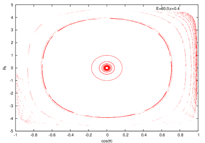
(a) Poincare map for $\epsilon=0.4$ and $E=60.0$ for the first 3 orders.

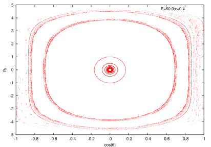
(b) Poincare map for $\epsilon=0.4$ and $E=60.0$ for the first 5 orders.

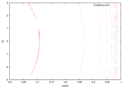
(c) Detail of the Poincare map for $\epsilon=0.4$ and $E=200.0$ for the first 3 orders.

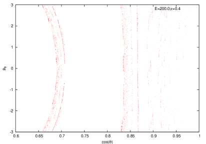
(d) Detail of the Poincare map for $\epsilon=0.4$ and $E=200.0$ for the first 5 orders.

Figure 1: Examples of Poincare maps for the dynamics near the Bradlow limit.

3.2 Dynamics of vortices in the plane ($\epsilon\rightarrow 1$ limit)

The dynamics of the Abelian Higgs model in $\mathbb{R}^{2}$ is a well studied problem, both analytically [Samols:1990kd, Samols:1991ne] and numerically [Moriarty:1988fx, Samols:1991ne]. Following the notation of Ref. [Samols:1991ne] we might write

$$ds^{2}=8F^{2}(2|u|)\ dud\overline{u}$$ (58)

Once the function $F(2|u|)$ is obtained, the dynamics in the geodesic approximation is completely determined. The form of the function $F(2|u|)$ has been deduced analytically for the special case of asymptotically separated vortices [Manton:2002wb], and has also been studied numerically several times[Samols:1990kd, Samols:1991ne]. In this paper we will use our expansion method to obtain a precise determination of $F(2|u|)$ for all values of $|u|$.

We will naturally assume that, if the torus is large enough compared both with the typical size of vortices, and with the distance between them, the dynamics will be accurately described by the one in $\mathbb{R}^{2}$. This means that, at least formally, we can calculate the desired function $F(2|u|)$ by taking the $\epsilon\longrightarrow 1$ limit while keeping $u$ fixed. At the beginning of this section we showed how to express the metric in the relative torus position coordinate $w$. The formula (Eq. 49) involves $\tilde{f}_{w}$ times a known function arising from the change of variables. We will first study the behaviour of the latter factor in the appropriate limit ($\epsilon\longrightarrow 1\,,\ u\ \text{fixed}$). Restricting to the $l_{1}=l_{2}=l$ case and recalling that $w=u\sqrt{2\pi(1-\epsilon)}$ we get:

$$\left(\frac{4\pi}{l}\right)^{2}|\vartheta_{4}(0)|^{4}\frac{|\vartheta_{1}(w)|^{2}|\vartheta_{4}(w)|^{2}}{\left(|\vartheta_{2}(w)|^{2}+|\vartheta_{3}(w)|^{2}\right)^{2}}\stackrel{{\scriptstyle\epsilon\rightarrow 1}}{{\longrightarrow}}\frac{16\pi^{2}Z_{2}^{2}}{(1+Z_{0}^{2})^{2}}(1-\epsilon)^{2}|u|^{2}$$ (59)

where $Z_{2}=-\frac{1}{2}\frac{\vartheta_{3}(0)\vartheta_{4}^{4}(0)}{\vartheta_{2}(0)}$, and $Z_{0}=-\vartheta_{3}(0)/\vartheta_{2}(0)$.

In summary, the function $F^{2}(2|u|)$ can be recovered as

$$F^{2}(2|u|)=\lim_{\epsilon\longrightarrow 1}\ (1-\epsilon)^{2}\tilde{f}_{w}(u\sqrt{2\pi(1-\epsilon)},\overline{u}\sqrt{2\pi(1-\epsilon)},\epsilon)\ \frac{2\pi^{2}Z_{2}^{2}}{(1+Z_{0}^{2})^{2}}|u|^{2}$$ (60)

In practice, to obtain an approximation to $F^{2}(2|u|)$ from our expansion we proceeded as follows. We computed the coefficients in the expansion in $\epsilon$ of the metric up to 40th order, for a regular rectangular array of points in the complex plane of the variable $w$. The range of values is that of a complex torus. Due to symmetries (which we checked) it is enough to take values in one quadrant. We considered a grid of $40\times 40$ points. Getting to order $40$ is feasible by implementing the iterative solution of the equations on a computer. This is possible using a Fourier expansion of the functions $h$ and $\dot{H}$ and truncating to a finite number of Fourier coefficients. One can tune this finite number until the precision attained in the function $\tilde{f}$ is of 14-16 decimal places. Due to the fast convergence of the Fourier coefficients, this procedure is not very costly. The computation in a conventional PC takes around 50 hours.

Once $\tilde{f}$ is determined at the grid points, in order to extract the values of $F^{2}(2|u|)$ we proceeded as follows. For a given value of $|u|$ we take many different values of $w$ from the grid and for each we compute the corresponding value of $\epsilon$. For that value we sum the series up to 40th order and multiply by the function associated to the change of variables (Eq. 49). Finally, for each value of $|u|$ we obtain we obtain a collection of numbers for different values of $\epsilon$ and for different phases of $u$. A typical case is displayed in Fig. 2, where we considered points having $|u|=1$ and situated along the diagonal $\mbox{Re}(u)=\mbox{Im}(u)$. The value of $F^{2}(2|u|)$ is the limit for $\epsilon$ approaching 1. Unfortunately, the larger values of $\epsilon$ are more seriously affected by the truncation of the series to 40 orders. This is exemplified by the errors attached to the points of the figure. These are obtained by subtracting the result obtained for 35 orders to that of 40 orders. To obtain a more precise determination of the value of $F(2|u|)$ we made two corrections. First of all, we partially corrected for the truncation errors by estimating the contribution of the terms from the 41st on. The precise way in which this is done will be explained later. This additional contribution does not affect significantly points for which the error obtained by comparing the 35th and 40th order is tiny. On the opposite extreme the contribution becomes unreliable when this error becomes very large. This occurs typically for values of $\epsilon$ exceeding $0.95$ (areas which are more than 20 times the critical area). We will therefore omit those points from our analysis.

To extract a good determination of $F^{2}(x)$ from our data we face the problem of extrapolating to $\epsilon=1$. This implies relating the results for a large torus with that of the plane. The torus case can be considered a solution of the plane with an infinite number of vortices – two per $l\times l$ cell. As the torus gets larger the replica vortices are increasingly far away, so that it is reasonable to use the analytic result for the case of a large number of asymptotically separated vortices to describe the approach. Using the result of Ref. [Manton:2002wb] we expect an additional contribution to the metric proportional to $\sum_{r}K_{0}(D_{r})$, where $K_{0}$ is the modified Bessel function of the second kind and $D_{r}$ is the distance to the replica vortex $r$. In the limit of large torus sizes and fixed $|u|$, this predicts a contribution proportional to $K_{0}(l)$. On the basis of the asymptotic behaviour of Bessel functions we decided to fit our data for each value of $u$ to a formula of the form

$$A-B(1-\epsilon)^{\frac{1}{4}}e^{-\sqrt{8\pi/(1-\epsilon)}}$$ (61)

For our $|u|=1$ example, the result is displayed by the solid line in Fig.2, and the fitted parameters are $B=145.0(5)$ and $A=F^{2}(2)=0.8791(4)$. The error reflects systematics due to changing the range of the fit as well as the relative weighting of the points. For other phases of $u$ we get compatible results. For example, for purely real or imaginary values of $u$ we obtain $F^{2}(2)=0.8800(6)$, consistent with rotational invariance.

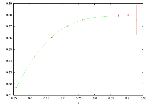
Figure 2: The points are the values of the left hand side of Eq. 60 for $|u|=1.0$ as a function of $\epsilon$, computed from the first 40 orders of our expansion. Error bars represent the size of the last 5 terms of the expansion. The solid line is a fit with Eq. 61.

Proceeding in the same way for several values of $|u|$ we arrive at the points displayed in Fig. 3. The errors are smaller than the size of the points in the figure. In all the range up to $|u|\geq 2$ the error is smaller than $6\;10^{-4}$ and for $|u|>0.5$ the relative error is smaller than 1 part in $10^{3}$.

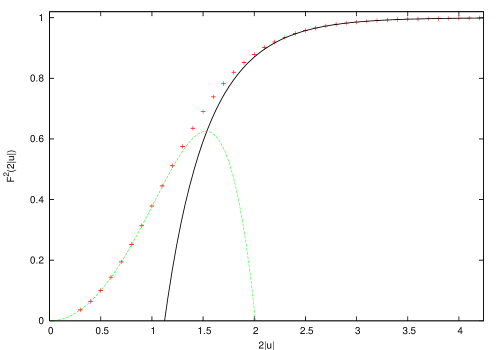
Figure 3: The metric computed using 40 orders of the Bradlow parameter expansion (red points), versus the $|u|\rightarrow 0$ approximation Eq. 66 (green dashed line) and the asymptotic form of the metric Eq. 67 (black solid line).

It is quite interesting to analyse the implications of the scaling limit for the coefficients of the $\epsilon$ expansion. For that purpose it is convenient to write $\epsilon=e^{-\delta}$ and replace the limit by $\delta\longrightarrow 0$. The condition that at large volumes the metric tends to that of the plane implies:

$$F^{2}(2|u|)=\lim_{\delta\rightarrow 0}\delta^{2}\frac{2\pi^{2}Z_{2}^{2}}{(1+Z_{0}^{2})^{2}}|u|^{2}\sum_{N=1}^{\infty}{\tilde{f}}^{(N)}(u\sqrt{2\pi\delta},\overline{u}\sqrt{2\pi\delta})e^{-N\delta}$$ (62)

It is clear that as $\delta$ tends to zero, more terms in the series become relevant. It is tempting to assume that the infinite sum tends to an integral over the variable $y=N\delta$. This would imply the following behaviour of the coefficients:

$$\lim_{N\longrightarrow\infty}{\tilde{f}}_{w}^{(N)}\left(u\sqrt{\frac{2\pi y}{N}},\overline{u}\sqrt{\frac{2\pi y}{N}}\right)\frac{\delta}{8}=h(|u|\sqrt{y})$$ (63)

In this case the limiting function $h(|u|\sqrt{y})$ would be related to $F^{2}(2|u|)$ as follows:

$$F^{2}(2|u|)=\frac{16\pi^{2}Z_{2}^{2}}{(1+Z_{0}^{2})^{2}}|u|^{2}\int_{0}^{\infty}e^{-y}h(|u|\sqrt{y})\,dy$$ (64)

which is essentially a Laplace transform.

With our results for ${\tilde{f}}_{w}^{(N)}$ up to $N=40$ and the set of values of $w$ spanning the aforementioned $40\times 40$ grid, we have analysed the validity of Eq. 63. For that purpose we plot in Fig. 4 the coefficients satisfying $35\leq N\leq 40$ and all values of $u$ in the range. The smoothness and thinness of the resulting curve, approximating $h(x)$, is a test of our scaling hypothesis. Errors, signalled by the spread of the values, grow with $x$. For example, including all coefficients $N>20$ would provide little changes in the thickness of the curve up to $x\approx 5$. Beyond, the thickness becomes a sizable fraction of the value.

The function $h(x)$ for small $x$, as determined from our results, fits nicely to a behaviour of the form

$$h(x)=a-bx^{4}+O(x^{5})$$ (65)

where $a=0.335(1)$ and $b=0.16(1)$. This expansion implies that for small values of the argument the metric function $F^{2}(2|u|)$ behaves as:

$$F^{2}(2|u|)=\frac{16\pi^{2}Z_{2}^{2}}{(1+Z_{0}^{2})^{2}}\left(a|u|^{2}-2b|u|^{6}\right)+O(|u|^{7})$$ (66)

The function on the left-hand side of the previous formula is displayed in Fig. 3. It matches nicely to the behaviour of the previously determined points (in red). For large values of $|u|$ the data also matches with the prediction coming from the asymptotic behaviour at large distances (Ref. [Manton:2002wb]) given by

$$F^{2}(2|u|)\stackrel{{\scriptstyle|u|\rightarrow\infty}}{{\longrightarrow}}1-8\sqrt{2}K_{0}(4|u|)$$ (67)

where $K_{0}(x)$ is the modified Bessel function of the second kind.

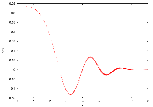
Figure 4: We plot the left-hand side of Eq. 63 for $N$ in the range 35-40, and fixed $x=|u|\sqrt{y}$.

To conclude we point out that our knowledge of $h(x)$ enables one to estimate the error introduced by the truncation in the number of terms in the $\epsilon$ expansion. For that one has simply to use the expression given in Eq. 64 with the integral restricted to $y>-N\log(\epsilon)$, where $N$ is the maximum order computed. We have tested this estimation with our data points and $N=40$. As mentioned previously, it improves the results for not too large values of $\epsilon$.

3.2.1 Scattering of vortices on the plane

Once the function $F(2|u|)$ has been obtained, it is trivial to compute the dynamics of the vortices. The Lagrangian, when written in polar coordinates $2u=re^{\imath\theta}$, is given by:

$$T=\pi F^{2}(r)\left[\dot{r}^{2}+r^{2}\dot{\theta}^{2}\right]$$ (68)

Since the energy is conserved, and we have rotational invariance ($p_{\theta}$ is also conserved), the system is integrable, and we have

$$\theta_{f}=\pi-\int^{\infty}_{r_{f}}\frac{dr}{r\sqrt{\frac{r^{2}}{b^{2}}F^{2}(2r)-1}}$$ (69)

where $b^{2}=\frac{\pi p_{\theta}^{2}}{4T}$ is the impact parameter. In particular, if we call $r_{m}$ the minimum distance between one vortex and the centre of mass during the trajectory, the scattering angle is given by

$$\theta_{sc}=\pi-2\int_{r_{m}}^{\infty}\frac{dr}{r\sqrt{\frac{r^{2}}{b^{2}}F^{2}(r)-1}}$$ (70)

Using our numerical data of Fig. 3 we can calculate these integrals. For values of $r>5$ we will use the asymptotic form of the metric, and for $r<0.5$ we can use our approximation Eq. (66). For the intermediate values we will use the cubic spline interpolating polynomial. In the Fig. 5 we have some examples of trajectories for different values of the impact parameter.

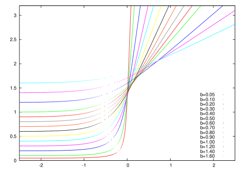
Figure 5: Scattering trajectories of two vortices.

We can also plot the scattering angle versus the impact parameter. The results are shown in Fig. 6. Errors were estimated in the following way. We generate a random set of values of $F(2|u|)$ assuming a Gaussian distribution around the central value and standard deviation fixed by the error. For each realization we compute the cubic spline interpolation polynomial and using it and the small and large approximation functions we compute the scattering angle for each impact parameter. The final errors are estimated on the basis of 1000 realizations. They are of the order of 1 part in $10^{4}$ or smaller.

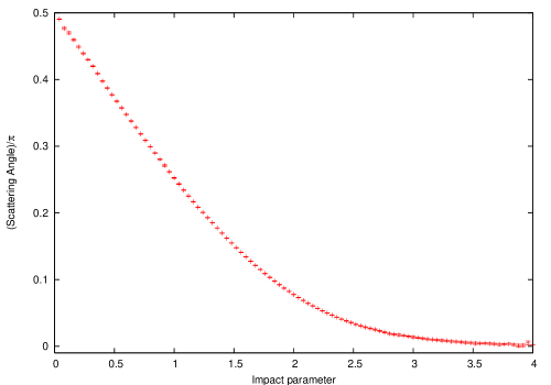
Figure 6: Scattering Angle vs. impact parameter.

4 Conclusions

In this paper we have shown how the Bradlow parameter expansion can be used to compute the metric of the moduli space of solutions of the Abelian Higgs model on the Torus. This extends our previous work [Gonzalez-Arroyo:2004xu] where this expansion was introduced as a tool to construct the classical vortex solutions on the Torus. More precisely, the expansion is performed in the variable $\epsilon=1-2f$, where $f$ is the average magnetic field. To any finite order in the expansion the metric has a known form depending on a small number of real parameters. We give their analytic expression up to second order for arbitrary number of vortices $q$. The leading term, giving the Bradlow limit result, is proportional to the Fubini-Study metric. This coincides with results obtained for the two-sphere [Baptista:2002kb]. The second order result depends on $q^{2}$ constants, which are given in the form of rapidly decreasing double infinite sums. Although increasingly complicated it is not too hard to go beyond this order. Rather than attempting this for the general vortex case, we have concentrated on the two-vortex case. We have given the form of the metric up to 5th order and the numerical value of their 15 real coefficients with 14-16 significant digits (machine double precision). Furthermore, it is possible to go much beyond this order in the computation of the metric at specific points of the moduli space by means of a computer. Essentially, the implementation is based on the truncation of the infinite sums to finite ones. In this way we have gone up to 40th order with fairly limited computational effort. Furthermore, the fast convergence of the sums stills maintains the double machine precision accuracy in the determination of the metric. Having so many terms in the expansion has allowed us to extrapolate our results to the infinite area case (vortices on the plane) with quite impressive results. The resulting metric is consistent with all the previously known results, both analytical in certain limits and numerical. The result have fairly small and controlled errors, arising from the extrapolation to infinite volume and the truncation in the expansion.

The computation of the metric allows the study of vortex scattering, known to be a good approximation up to relatively high vortex velocities. The presence of the torus can be used to mimic the behaviour of vortices in a dense environment. A natural question that poses itself is the possibility that two-vortex dynamics on the torus is integrable. This is actually the case for both small (close to critical) torus sizes as for infinitely large ones (the plane). We have analysed Poincare maps as a first step in this study. Furthermore, we emphasise that, as in our previous work, our method has been found to be a competitive tool to study the properties of vortices on the plane. It has important advantages over other methods: its semi-analytical nature and the possibility of dealing with an arbitrary number of vortices. In this work, for example, we have given the curves (with errors) that describe the functional dependence of the two-vortex scattering angle with the impact parameter.

To conclude, we want to mention that the Bradlow expansion method is generalisable to many other cases and theories. For example, it can be applied to any other two-dimensional compact manifold. Furthermore, a similar expansion seems to apply in other cases where a Bradlow parameter can be introduced [Bradlow:1990ir], such as abelian and non-abelian gauge-Higgs theories in Kähler manifolds of arbitrary dimensionality. The methodology can be extended beyond. For example, a related expansion, is known to exist in the study of self-dual configurations on the 4 dimensional torus [GarciaPerez:2000yt]. Recently [Forgacs:2005ct, Lozano:2006xn], it has also been applied to the study of abelian vortices in a non commutative torus. In all these theories, apart from the determination of the shape of the solutions and the form of the metric of the moduli space, other problems can be attacked. In particular, one can study the eigenfunctions and eigenvalues of the Dirac operator in a vortex background and also compute quantum corrections to the vortex. These problems are currently under study by the present authors.

Appendix A Apendix:

To lowest order we have that $h^{(0)}=\ln(||c||)$ and $\dot{H}^{(0)}=\frac{\sum_{i}\overline{c}_{i}\dot{c}_{i}}{||c||^{2}}$ are constant. The symbol $||c||^{2}$ stands for $\sum_{i}|c_{i}|^{2}$. Hence, the lowest order metric is given by

$$g^{(1)}_{ij}=\frac{{\cal A}}{\pi||c||^{2}}\left(\delta_{ij}-\frac{\overline{c}_{i}c_{j}}{||c||^{2}}\right)$$ (71)

The matrix inside parenthesis, which we will call ${\mathcal{P}}$, is the orthogonal projector to the vector $c_{i}$. It gives precisely the Fubini-Study metric written in homogeneous coordinates.

To the next order the metric, written in matrix notation, adopts the form:

$$g^{(2)}=\frac{{\cal A}}{\pi||c||^{2}}\ {\mathcal{P}}\left(-{\mathbf{I}}\frac{\sum_{ij}\overline{c}_{i}\overline{S}_{ij}c_{j}}{||c||^{2}}+\overline{S}+\widetilde{S}\right){\mathcal{P}}$$ (72)

where

$$\overline{S}_{ij}=\frac{\overline{c}_{l}c_{k}}{{\mathcal{A}}||c||^{2}}\int d^{2}x\overline{\chi}_{i}\chi_{j}\Delta^{-1}(\overline{\chi}_{l}\chi_{k})^{\prime}$$ (73)

and

$$\widetilde{S}_{ij}=\frac{\overline{c}_{l}c_{k}}{{\mathcal{A}}||c||^{2}}\int d^{2}x\overline{\chi}_{i}\chi_{k}\Delta^{-1}(\overline{\chi}_{l}\chi_{j})^{\prime}$$ (74)

The prime denotes the removal of the constant Fourier mode, making the inverse laplacian $\Delta^{-1}$ well-defined.

The computation of the integrals can be explicitly carried over by using Fourier transforms. For that purpose we introduce the quantities:

$$L^{ij}(\vec{n})=\frac{1}{\mathcal{A}}\int_{\mathbb{T}^{2}}d^{2}x\,\overline{\chi}_{i}e^{-2\pi\imath n_{i}\cdot\frac{x_{i}}{l_{i}}}\chi_{j}$$ (75)

which are just the Fourier modes of the product $\overline{\chi}_{i}\chi_{j}$. Now we remove the constant mode ($\vec{n}=0$) and denote the result as $L^{\prime ij}(\vec{n})$. Then the integral entering in the definition of $\overline{S}$ and $\widetilde{S}$ is given by

$$S_{ijkl}\equiv-\frac{1}{\mathcal{A}}\int_{\mathbb{T}^{2}}d^{2}x\overline{\chi}_{i}\chi_{j}\Delta^{-1}(\overline{\chi}_{l}\chi_{k})^{\prime}=\sum_{\vec{n}}\frac{L^{\prime ij}(\vec{n})L^{\prime lk}(-\vec{n})}{\xi(\vec{n})}$$ (76)

where

$$\xi(\vec{n})=\frac{\pi\tau}{q}\left[n_{1}^{2}+\frac{n_{2}^{2}}{\tau^{2}}\right]$$ (77)

and $\tau=l_{2}/l_{1}$. The explicit value of the coefficients depends on the choice of basis. For the choice given earlier $\chi_{s+1}=\Psi_{0s}$ defined in equation $(A.24)$ of our previous paper [Gonzalez-Arroyo:2004xu], the coefficients are given (as a particular case) of Eq. (A.30) of that paper. The matrix ${\mathbf{L}}(\vec{n})$ becomes:

$${\mathbf{L}}(n)={\mathbf{\Gamma}}(\vec{n})e^{-\frac{\xi(\vec{n})}{2}}$$ (78)

where the matrices ${\mathbf{\Gamma}}(\vec{n})$ are defined as

$${\mathbf{\Gamma}}(\vec{n})=P^{n_{1}}Q^{n_{2}}e^{-\imath\pi\frac{n_{1}n_{2}}{q}}$$ (79)

where $P$ and $Q$ are ‘t Hooft $q\times q$ matrices ($P_{ij}=\delta_{ji+1}$, $Q=\mbox{\rm diag}(\exp{2\pi is/q})$). The matrices ${\mathbf{\Gamma}}(\vec{n})$ are unitary and satisfy ${\mathbf{\Gamma}}^{\dagger}(\vec{n})={\mathbf{\Gamma}}(-\vec{n})$. From here one realises that, the coefficients $S_{ijkl}$ can be expressed in terms of $q^{2}$ constants $K(\vec{s})$ as follows:

$$S_{ijkl}=\sum_{\vec{s}}K(\vec{s})\,\Gamma_{ij}(\vec{s})\,\Gamma_{kl}(\vec{-s})$$ (80)

where $\vec{s}$ is a 2 component vector with components $s_{i}\in\{0,\ldots,q-1\}$. From Eq. 76 one derives:

$$K(\vec{s})=\sum_{\vec{k}\in Z^{2}}\frac{e^{-\xi(\vec{s}+q\vec{k})}}{\xi(\vec{s}+q\vec{k})}=\int_{1}^{\infty}d\alpha\left(\vartheta\left[\begin{array}[]{c}s_{1}/q\\ 0\end{array}\right](0|iq\alpha\tau)\;\vartheta\left[\begin{array}[]{c}s_{2}/q\\ 0\end{array}\right](0;iq\alpha/\tau)-1\right)$$ (81)

The terms in the sum decay exponentially with $k^{2}$, so that a few terms in the infinite sums over $\vec{k}$ suffice to obtain a very high accuracy.

The matrices ${\mathbf{\Gamma}}(\vec{s})$ are a basis of the set of $q\times q$ matrices. Hence, it is possible to express the metric tensor to this order as a linear combination of these matrices. The coefficients are functions of the following quadratic forms in $c_{i}/||c||$:

$$P(\vec{s})=\frac{\overline{c}{\mathbf{\Gamma}}(-\vec{s})c}{||c||^{2}}$$ (82)

These are not independent, and satisfy certain relations. In particular one has $P(\vec{0})=1$ and

$$\sum_{\vec{s}\neq\vec{0}}|P(\vec{s})|^{2}=q-1$$ (83)

As an example, we give the explicit expression for the trace of $g^{(2)}$:

$$||c||^{2}{\rm Tr}(g^{(2)})=\frac{{\cal A}}{\pi}\ \sum_{\vec{s}\neq\vec{0}}K(\vec{s})((q+1)|P(\vec{s})|^{2}-1)$$ (84)

From here it is trivial to reproduce the $q=2$ case given in section 3.1. Notice that $(P(1,0),P(0,1),P(1,1))$ is a 3-component unit vector whose expression in terms of spherical coordinates coincides with our definition of $\theta$ and $\varphi$ in Eq. 44. For the symmetric $l_{1}=l_{2}$ case we obtain

$$\tilde{f}^{(2)}=\frac{{\cal A}}{\pi}\ (K(1,0)-K(1,1))(1-3|P(1,1)|^{2})$$ (85)

where $P(1,1)=\cos\theta$. This reproduces the result given in Table 1. Notice that the result is proportional to the second Legendre polynomial in $\cos{\theta}$ as follows from the area condition.

Going over to higher orders is tedious but presents essentially no new difficulties. We have obtained the analytic result to third order for the $q=2$, $\tau=1$ case, matching the value given in Table 1.