Fermions on Colliding Branes

Abstract

We study the behaviour of five-dimensional fermions localized on branes, which we describe by domain walls, when two parallel branes collide in a five-dimensional Minkowski background spacetime. We find that most fermions are localized on both branes as a whole even after collision. However, how much fermions are localized on which brane depends sensitively on the incident velocity and the coupling constants unless the fermions exist on both branes.

I introduction

It has been known since the 70’s that topological defects such as domain walls can trap fermions on their world volumes Jackiw_Rebbi . In the 80’s this fact formed an integral part of suggestions that one may regard our universe as a domain wall Akama ; Rubakov_Shaposhnikov ; Visser ; Gibbons_Wiltshire , or more generally a brane in a higher dimensional universe Arkani ; Randall_Sundrum ; Binetruy_Deffayet_Langlois ; Shiromizu_Maeda_Sasaki . The idea is that the fermionic chiral matter making up the standard model is composed of such trapped zero modes Gherghetta ; Bajc_Gabadadze ; Daemi_Shaposhnikov ; Dubovsky_Rubakov_Tinyakov ; Kehagias_Tamvakis ; Ringeval_Peter_Uzan ; Koley_Kar ; Melfo_Pantoja_Tempo . A similar mechanism is used in models, such as the Horawa-Witten model Horava_Witten ; Lukas-Ovrut-Waldram of heterotic M-Theory, in which two domain walls are present. Our world is localized on one brane and a shadow world is localized on the other brane. The existence of models with more than one brane suggests that branes may collide, and it is natural to suppose that the Big Bang is associated with the collision Khoury_Ovrut_Steinhardt_Turok ; Steinhardt_Turok . This raises the fascinating questions of what happens to the localized fermions during such collisions? Put more picturesquely, what is the fate of the standard model during brane collision? In this paper we shall embark on what we believe is the first study of this question by solving numerically the Dirac equation for a fermions coupled via Yukawa interaction to a system of two colliding domain walls, i.e. a kink-anti-kink collision in five-dimensional Minkowski spacetime. Each individual domain wall may be described analytically by a static solution and given such a solution one may easily find analytically the fermion zero modes, which from the point of view of the 3+1 dimensional world volume behave like massless chiral fermions. The back reaction of the fermions on the domain wall is here, and throughout this paper, neglected.

Kink-anti-kink collisions, have recently been studied numerically Anninos_Oliveira_Matzner ; Takamizu_Maeda1 ; Copeland . One solves the scalar field equations with initial data corresponding to a superposition of the boosted profiles of a kink and an anti-kink. It was found Anninos_Oliveira_Matzner ; Takamizu_Maeda1 that, depending on the initial relative velocity that such domain wall pairs can pass through one another, or bounce, or suffer a number of bounces in a fashion reminiscent of the cyclic universe scenario Steinhardt_Turok . One may extend the treatment to include gravity Langlois_Maeda_Wands ; Takamizu_Maeda2 ; Gibbons_Lu_Pope ; Chen_Chong_Gibbons_Lu_Pope ; McFadden_Turok_Steinhardt but in this paper we shall, for the sake of our preliminary study, work throughout with gravity switched off. One may now solve the Dirac equation in the time dependent background generated by the kink-anti-kink collision. We use as initial data for the Dirac equation the boosted profiles of the chiral zero modes associated with the individual domain walls.

What we find was for us unexpected and quite remarkable. If the initial fermions exist on both branes, then without exception, for a whole range of initial conditions, the two initially distinct but localized fermion distributions merge in the neighborhood of the collision, and then emerge after the collision again localized on one or the other kink. By contrast if one of the kinks is empty, which we refer to as a vacuum brane, then the amplitudes of the fermions on the kinks after the collision highly depend on the incident velocity and the coupling constants.

II Fermions on moving branes

II.1 Fermion with Yukawa coupling and its symmetry

We start with a discussion of five-dimensional (5D) four-component fermions in a time-dependent domain wall in 5D Minkowski spacetime. As a domain wall, we adopt a 5D real scalar field $\Phi$ with an appropriate potential $V(\Phi)$. The 5D Dirac equation with a Yukawa coupling term $g\Phi\bar{\Psi}\Psi$ is given by

$$(\Gamma^{\hat{A}}\partial_{\hat{A}}+g\Phi)\Psi=0,~{}~{}~{}(\hat{A}=0,1,2,3,5)\,,$$ (1)

where $\Psi$ is a 5D four-component fermion. $\Gamma^{\hat{A}}$ are the Dirac matrices in 5D Minkowski spacetime satisfying the anticommutation relations,

$$\{\Gamma^{\hat{A}},\Gamma^{\hat{B}}\}=2\eta^{\hat{A}\hat{B}}\,,$$ (2)

where $\eta^{\hat{A}\hat{B}}={\rm diag}(-1,1,1,1,1)$ is Minkowski metric. We explicitly use the following Dirac-Pauli representation

$${\Gamma}^{\hat{0}}=\left(\begin{array}[]{cc}-i&0\\ 0&i\end{array}\right),~{}~{}{\Gamma}^{\hat{5}}=\left(\begin{array}[]{cc}0&1\\ 1&0\end{array}\right)\,,$$ (7)

$${\Gamma}^{\hat{k}}=\left(\begin{array}[]{cc}0&-i\sigma^{k}\\ i\sigma^{k}&0\end{array}\right),~{}~{}(k=1,2,3)\,,~{}~{}$$ (10)

with $\sigma^{k}$ being the Pauli $2\times 2$ matrices.

Note that Eq. (1) implies current conservation law:

$$\partial_{A}n^{A}=0\,,$$ (11)

where $n^{A}\equiv\bar{\Psi}\Gamma^{\hat{A}}\Psi$ is conserved number current. Here we define $\bar{\Psi}\equiv\Psi^{\dagger}\Gamma_{\hat{0}}$. This gives conserved number density $n\equiv n^{0}=\bar{\Psi}\Gamma^{\hat{0}}\Psi=\Psi^{\dagger}\Psi$. The total number of fermions is defined by $N=\int d^{5}Xn$, which is conserved.

Later we shall need the fact that the Dirac equation (1) has the following time reversal and reflection symmetries:
(1) If $\Psi(t,\vec{x},z)$ is a solution of the Dirac equation with scalar field $\Phi(t,\vec{x},z)$, $\Gamma^{\hat{0}}\Psi(-t,\vec{x},z)$ is a solution of the Dirac equation with the scalar field $-\Phi(-t,\vec{x},z)$, where $X^{5}=z$ is the coordinate of a fifth dimension. In particular, when there is no interaction ($\Phi=0$ or $g=0$), $\Gamma^{\hat{0}}\Psi(-t,\vec{x},z)$ is time reversal of $\Psi(t,\vec{x},z)$
(2) If $\Psi(t,\vec{x},z)$ is a solution of the Dirac equation with scalar field $\Phi(t,\vec{x},z)$, $\Gamma^{\hat{5}}\Psi(t,\vec{x},-z)$ is a solution of the Dirac equation with the scalar field $-\Phi(t,\vec{x},-z)$. In particular, if $\Psi(t,\vec{x},z)$ is a solution for a kink [an anti-kink], $\Gamma^{\hat{5}}\Psi(t,\vec{x},z)$ is a solution for an anti-kink [a kink]. It will turn out that the solution with a kink [an anti-kink] is related to positive [negative] chiral fermions, which are defined below (see next subsection).
(3) Combining (1) and (2), we find that $\Gamma^{\hat{5}}\Gamma^{\hat{0}}\Psi(-t,\vec{x},-z)$ is a solution of the Dirac equation with $\Phi(-t,\vec{x},-z)$

If we assume some symmetries for a domain wall, we find further properties for fermions as follows.
(i) For the case of a static domain wall, (1) yields that $\Gamma^{\hat{0}}\Psi(t,\vec{x},z)$ is a solution for an anti-kink [a kink] if $\Psi(t,\vec{x},z)$ is a solution for a kink [an anti-kink].
(ii) If a domain wall is described by a kink (or an anti-kink), which has symmetry such that $\Phi(t,\vec{x},-z)=-\Phi(t,\vec{x},z)$, (2) yields that $\Gamma^{\hat{5}}\Psi(t,\vec{x},z)$ is a solution for an anti-kink [a kink] if $\Psi(t,\vec{x},z)$ is a solution for a kink [an anti-kink].
(iii) We may also have time symmetry such that $\Phi(-t,\vec{x},z)=\Phi(t,\vec{x},z)$ for collision of two walls. In fact we find from numerical analysis that this ansatz is approximately correct Takamizu_Maeda1 . Assuming $z$-reflection symmetry as well, we find from (3) that $\Gamma^{\hat{5}}\Gamma^{\hat{0}}\Psi_{\pm}(-t,\vec{x},-z)$, which is time reversal and $z$-reflection of $\Psi_{\pm}(t,\vec{x},z)$, is also a solution for the same scalar field $\Phi(t,\vec{x},z)$.

Before going to analyze concrete examples, we introduce two chiral fermion states

$$\Psi_{\pm}={1\over 2}\left(1\pm{\Gamma}^{\hat{5}}\right)\Psi$$ (12)

This definition implies

$${1\over 2}\left(1\pm{\Gamma}^{\hat{5}}\right)\Psi_{\pm}=\Psi_{\pm},~{}{1\over 2}\left(1\mp{\Gamma}^{\hat{5}}\right)\Psi_{\pm}=0\,.$$ (13)

Using the representation (10), we have

$$\Psi_{+}=\left(\begin{array}[]{c}\psi_{+}\\ \psi_{+}\end{array}\right)\,,~{}~{}\Psi_{-}=\left(\begin{array}[]{c}\psi_{-}\\ -\psi_{-}\end{array}\right)\,,$$ (18)

where $\psi_{+}$ and $\psi_{-}$ are two-component spinors.

The Dirac equation (1) is now reduced to

$$\left(\pm\partial_{\hat{5}}+g\Phi\right)\psi_{\pm}+\Gamma^{\hat{\mu}}\partial_{\hat{\mu}}\psi_{\mp}=0\,.$$ (19)

II.2 Fermions on a kink (or an anti-kink)

As for a domain wall, now we assume the potential form is given by $V(\Phi)={\lambda\over 4}\left(\Phi^{2}-\eta^{2}\right)^{2}$. Here we recall the dimension of some variables. Since we discuss five dimensional spacetime, we have the following dimensionality:

$$[\Phi]=[\eta]=L^{-3/2},[\Psi]=L^{-2},[g]=L^{1/2},[\lambda]=L\,,$$ (20)

where $L$ is a scale length. In what follows, we use units in which $m_{\eta}(\equiv\eta^{2/3})=1$.

Then a domain wall solution is given by

$$\Phi=\epsilon\tanh\left({z\over D}\right)\,,$$ (21)

where $\epsilon=\pm$ correspond to a kink and an anti-kink solutions and $D=\sqrt{2/\lambda}$ is the width of a domain wall. Note that $\Phi(z)$ is an odd function of $z$.

As for a fermion, in the case of a static domain wall, separating variables as $\psi_{+}=\mbox{{$\stackrel{{\scriptstyle\mbox{\tiny(4)}}}{{\textstyle\psi}}$}}_{+}(x^{\mu})f_{+}(z)$ and $\psi_{-}=\mbox{{$\stackrel{{\scriptstyle\mbox{\tiny(4)}}}{{\textstyle\psi}}$}}_{-}(x^{\mu})f_{-}(z)$ and assuming massless chiral fermions on a brane, i.e. $\Gamma^{\hat{\mu}}\partial_{\mu}\mbox{{$\stackrel{{\scriptstyle\mbox{\tiny(4)}}}{{\textstyle\psi}}$}}_{\pm}(x^{\mu})=0$, we find the equations for $f_{\pm}(z)$ as

$$\left(\pm\partial_{5}+g\Phi(z)\right)f_{\pm}=0$$ (22)

With Eq. (21), we find the solutions are

$$f_{\pm}\propto\left[\cosh\left({z\over D}\right)\right]^{\mp\epsilon gD}\,.$$ (23)

Note that the fermion wave function is an even function of $z$. Hence the positive-chiral (the negative-chiral) fermion is localized for a kink (an anti-kink ) but is not localized for an anti-kink (a kink).

To fix numbers of fermions on a wall, $f_{\pm}$ should be normalized up to an arbitrary phase factor $\phi_{\pm(0)}$, which is set to be zero. Using a number density of fermions given by

$$n\equiv\Psi^{\dagger}\Psi=2\left(\psi_{+}^{\dagger}\psi_{+}+\psi_{-}^{\dagger}\psi_{-}\right)\,,$$ (24)

we normalize the total number of fermions localized on a static domain wall to be unity, i.e. $N=1$. More precisely, for a kink (an anti-kink), we impose

$$\int_{-\infty}^{\infty}n_{\pm}d\tilde{z}=1\,,$$ (25)

which gives

$$f_{\pm}(z)=\left[{\Gamma(gD+{1\over 2})\over 2\sqrt{\pi}D\Gamma(gD)}\right]^{1/2}\left[\cosh\left({z\over D}\right)\right]^{-gD}\,.$$ (26)

Using this solution, we can describe the wave function of fermion localized on a kink (or an anti-kink) as

$$\Psi^{(\rm K)}(x,z)=\left(\begin{array}[]{c}\mbox{{$\stackrel{{\scriptstyle\mbox{\tiny(4)}}}{{\textstyle\psi}}$}}_{+}(x)f_{+}(z)\\ \mbox{{$\stackrel{{\scriptstyle\mbox{\tiny(4)}}}{{\textstyle\psi}}$}}_{+}(x)f_{+}(z)\end{array}\right)\,,$$ (29)

$$\Psi^{(\rm A)}(x,z)=\left(\begin{array}[]{c}\mbox{{$\stackrel{{\scriptstyle\mbox{\tiny(4)}}}{{\textstyle\psi}}$}}_{-}(x)f_{-}(z)\\ -\mbox{{$\stackrel{{\scriptstyle\mbox{\tiny(4)}}}{{\textstyle\psi}}$}}_{-}(x)f_{-}(z)\end{array}\right)\,.$$ (32)

To quantize the fermion fields, we define annihilation operators of localized fermions on a kink and on an anti-kink by

$$a_{\rm K}=\langle\Psi^{(\rm K)},\Psi\rangle~{}~{}{\rm and}~{}~{}a_{\rm A}=\langle\Psi^{(\rm A)},\Psi\rangle$$ (33)

Note that those two states are orthogonal, i.e. $\langle\Psi^{(\rm K)},\Psi^{(\rm A)}\rangle=0$.

II.3 Fermion wave function on a moving domain wall

To discuss fermions at collision of branes, we first discuss fermions on a domain wall moving with a constant velocity. When a domain wall is moving, however, $\Phi$ is time-dependent, and then the above prescription (separation of the fifth coordinate) to find wave functions is no longer valid.

Since 3-space is flat, we expand the wave functions by Fourier series as

$$\psi_{\pm}={1\over(2\pi)^{3/2}}\int d^{3}\vec{k}~{}e^{i\vec{k}\vec{x}}\psi_{\pm}(t,z;\vec{k})\,.$$ (34)

We find the Dirac equations become

$$\left(\pm\partial_{5}+g\Phi\right)\psi_{\pm}-\left(i\partial_{0}\pm(\vec{k}\cdot\vec{\sigma})\right)\psi_{\mp}=0\,.$$ (35)

In what follows, we shall consider only low energy fermions, that is, we assume that $\vec{k}\approx 0$, that is $|\vec{k}|$ is enough small compared with the mass scale of 5D fermion ($g\Phi$). The equations we have to solve are now

$$i\partial_{0}\psi_{\pm}=\left(\mp\partial_{5}+g\Phi\right)\psi_{\mp}\,.$$ (36)

Since up- and down-components of $\psi_{\pm}$ are decoupled, we discuss only up-components here. Note that taking into account $\vec{k}$ mixes the up- and down-components. With this ansatz, we can describe fermion by two single-component chiral wave functions as

$$\Psi=\left(\begin{array}[]{c}1\\ 0\\ 1\\ 0\end{array}\right)\psi_{+}(z,t)+\left(\begin{array}[]{c}1\\ 0\\ -1\\ 0\end{array}\right)\psi_{-}(z,t)\,.$$ (45)

For a localized fermion on a static kink (or an anti-kink), the wave functions are $\psi_{\pm}(z,t)=f_{\pm}(z)$.

Next we construct a localized fermion wave function on a moving domain wall with a constant velocity $\upsilon$. In this case, we can find the analytic solution by a Lorentz boost. We find for a kink with velocity $\upsilon$,

$$\psi_{+}^{(\rm K)}(z,t;\upsilon) = \sqrt{\gamma+1\over 2}\tilde{\psi}^{(\rm K)}\left({\gamma(z-\upsilon t)}\right)\,,$$ (46)

$$\psi_{-}^{(\rm K)}(z,t;\upsilon) = i{\gamma\upsilon\over\gamma+1}\sqrt{\gamma+1\over 2}\tilde{\psi}^{(\rm K)}\left({\gamma(z-\upsilon t)}\right)$$

and for an anti-kink with velocity $\upsilon$,

$$\psi_{-}^{(\rm A)}(z,t;\upsilon) = \sqrt{\gamma+1\over 2}\tilde{\psi}^{(\rm A)}\left({\gamma(z-\upsilon t)}\right)\,,$$ (47)

$$\psi_{+}^{(\rm A)}(z,t;\upsilon) = -i{\gamma\upsilon\over\gamma+1}\sqrt{\gamma+1\over 2}\tilde{\psi}^{(\rm A)}\left({\gamma(z-\upsilon t)}\right)$$

where $\tilde{\psi}^{(\rm K)}(\tilde{z})=f_{+}(\tilde{z})$ and $\tilde{\psi}^{(\rm A)}(\tilde{z})=f_{-}(\tilde{z})$ are static wave functions of chiral fermions localized on static kink and anti-kink, respectively, and $\gamma=1/\sqrt{1-\upsilon^{2}}$ is the Lorentz factor.

We can check that the total number of fermions is preserved also in the boosted Lorentz frame. From Eqs. (46) and (47), we find that $n=\gamma\tilde{n}$. Integrating it in the $z$-direction, we find

$$\int_{t={\rm const}}dz~{}n = \int_{t={\rm const}}dz~{}\gamma\tilde{n}\left(\gamma(z-vt)\right)$$ (48)

$$= \int d\tilde{z}~{}\tilde{n}\left(\tilde{z}\right)=1\,.$$

If a domain wall is given by a kink [an anti-kink], we have only the positive-chiral fermions in a comoving frame [the negative-chiral fermions]. However, from Eqs (46) and (47), we find that the negative-chiral modes [positive-chiral modes] also appear in this boosted Lorentz frame. For a kink, the ratio of number density of the negative-chiral modes to that of the positive-chiral ones is given by $\gamma^{2}\upsilon^{2}/(\gamma+1)^{2}$.

The above wave functions on a moving domain wall with constant velocity can be used for setting the initial data for colliding domain walls.

III Fermions on colliding domain wall

III.1 Initial setup

We construct our initial data as follows. Provide a kink solution at $z=-z_{0}$ and an anti-kink solution at $z=z_{0}$, which are separated by a large distance and approaching each other with the same speed $\upsilon$. We can set up as an initial profile for the scalar field $\Phi$:

$$\Phi(z,t)=\Phi^{\rm(K)}(z,t;\upsilon)+\Phi^{\rm(A)}(z,t;-\upsilon)-1\,,$$ (49)

where

$$\Phi^{\rm(K,A)}(z,t;\upsilon) =\pm\tanh(\gamma(z-\upsilon t)/D)$$ (50)

are the Lorentz boosted kink and anti-kink solutions, respectively. Here we have chosen that the initial time is $t=t_{\rm in}\equiv-z_{0}/\upsilon$. The domain walls collide at $t=0$.

For fermions on moving walls, we first expand the wave function as

$$\hat{\Psi}=\Psi_{\rm in}^{(\rm K)}(x,z;\upsilon)a_{\rm K}+\Psi_{\rm in}^{(\rm A)}(x,z;-\upsilon)a_{\rm A}+\Psi_{\rm in}^{(\rm B)}(x,z)a_{\rm B}\,,$$ (51)

where $\Psi_{\rm in}^{(\rm K)}(x,z;\upsilon)$ and $\Psi_{\rm in}^{(\rm A)}(x,z;-\upsilon)$ are the wave function of right-moving localized fermion on a kink and those of left-moving one on an anti-kink, respectively, which are explicitly by Eq. (46) and Eq. (47). We also denote the bulk fermions symbolically by $\Psi_{\rm in}^{(\rm B)}(x,z)$. We do not give its explicit form because it does not play any important role in the present situation. We have assumed in Eq. (51) that $\{\Psi_{\rm in}^{(\rm K)}(x,z;\upsilon),\Psi_{\rm in}^{(\rm A)}(x,z;-\upsilon)$ and $\Psi_{\rm in}^{(\rm B)}(x,z)\}$ form a complete orthogonal system. Note that $\{\Psi_{\rm in}^{(\rm K)}(x,z;\upsilon)$ and $\Psi_{\rm in}^{(\rm A)}(x,z;-\upsilon)\}$ are orthogonal.

Now we can set up an initial state for fermion by creation-annihilation operators. We shall call a domain wall associated with fermions a fermion wall, and a domain wall in vacuum a vacuum wall. We shall discuss two cases: one is collision of two fermion walls, and the other is collision of fermion and vacuum walls. For initial state of fermions, we consider two states;

$$|{\rm KA}\rangle \equiv a_{\rm A}^{\dagger}a_{\rm K}^{\dagger}|0\rangle\,$$ (52)

$$|{\rm K}0\rangle \equiv a_{\rm K}^{\dagger}|0\rangle\,$$ (53)

where $|0\rangle$ is a fermion vacuum state.

III.2 Outgoing states and expectation values

We discuss behaviour of fermions at collision. After collision of two domain walls, each wall will recede to infinity with almost the same velocity as the initial one $\upsilon$. Therefore we expect that positive chiral fermions stay on a left-moving kink and negative ones on a right-moving anti-kink. Those wave functions are given by $\Psi_{\rm out}^{(\rm K)}(x,z;-\upsilon)$ and $\Psi_{\rm out}^{(\rm A)}(x,z;\upsilon)$. There may be bulk fermions which are left behind after collision, which wave function is symbolically written by $\Psi_{\rm out}^{(\rm B)}(x,z)$. Since the initial wave functions ($\Psi_{\rm in}^{(\rm K)}(x,z;\upsilon)$ and $\Psi_{\rm in}^{(\rm A)}(x,z;-\upsilon)$) are described by the finial wave functions ($\Psi_{\rm out}^{(\rm K)}(x,z;-\upsilon)$, $\Psi_{\rm out}^{(\rm A)}(x,z;\upsilon)$, and $\Psi_{\rm out}^{(\rm B)}(x,z)$ at $t=t_{\rm out}\equiv z_{0}/\upsilon$), we find the relations between them by solving the Dirac equation (36). Those relations can be written as

$$\Psi_{\rm in}^{(\rm K)}(x,z;\upsilon) \sim \alpha_{\rm K}\Psi_{\rm out}^{(\rm K)}(x,z;-\upsilon)+\beta_{\rm K}\Psi_{\rm out}^{(\rm A)}(x,z;\upsilon)$$ (54)

$$+\gamma_{\rm K}\Psi_{\rm out}^{(\rm B)}(x,z)\,,$$

$$\Psi_{\rm in}^{(\rm A)}(x,z;-\upsilon) \sim \alpha_{\rm A}\Psi_{\rm out}^{(\rm A)}(x,z;\upsilon)+\beta_{\rm A}\Psi_{\rm out}^{(\rm K)}(x,z;-\upsilon)$$ (55)

$$+\gamma_{\rm A}\Psi_{\rm out}^{(\rm B)}(x,z)\,.$$

In order to define final fermion states, we also describe the wave function as

$$\hat{\Psi}=\Psi_{\rm out}^{(\rm K)}(x,z;-\upsilon)b_{\rm K}+\Psi_{\rm out}^{(\rm A)}(x,z;\upsilon)b_{\rm A}+\Psi_{\rm out}^{(\rm B)}(x,z)b_{\rm B}\,,$$ (56)

where $b_{\rm K}$, $b_{\rm A}$ and $b_{\rm B}$ are annihilation operators of those fermion states. From Eqs. (51), (54), (55) and (56), we find

$$b_{\rm K} =\alpha_{\rm K}a_{\rm K}+\beta_{\rm A}a_{\rm A}\,,$$ (57)

$$b_{\rm A} =\alpha_{\rm A}a_{\rm A}+\beta_{\rm K}a_{\rm K}$$ (58)

Using the Bogoliubov coefficients $\alpha_{\rm K},\beta_{\rm K}$ and $\alpha_{\rm A},\beta_{\rm A}$, we obtain the expectation values of fermion number on a kink and an anti-kink after collision as

$$\langle N_{\rm K}\rangle\equiv\langle{\rm KA}|b_{\rm K}^{\dagger}b_{\rm K}|{\rm KA}\rangle=|\alpha_{\rm K}|^{2}+|\beta_{\rm A}|^{2}\,$$ (59)

$$\langle N_{\rm A}\rangle\equiv\langle{\rm KA}|b_{\rm A}^{\dagger}b_{\rm A}|{\rm KA}\rangle=|\alpha_{\rm A}|^{2}+|\beta_{\rm K}|^{2}$$ (60)

for the case of $|{\rm KA}\rangle$. If the initial state is $|{\rm K}0\rangle$, we find

$$\langle N_{\rm K}\rangle \equiv\langle{\rm K}0|b_{\rm K}^{\dagger}b_{\rm K}|{\rm K}0\rangle=|\alpha_{\rm K}|^{2}\,$$ (61)

$$\langle N_{\rm A}\rangle \equiv\langle{\rm K}0|b_{\rm A}^{\dagger}b_{\rm A}|{\rm K}0\rangle=|\beta_{\rm K}|^{2}\,.$$ (62)

III.3 Time evolution of fermion wave functions

In order to obtain the Bogoliubov coefficients, we have to solve the equations for domain wall $\Phi$Takamizu_Maeda1 and fermion $\Psi$ numerically. For the time evolution of $\Psi$, we use the Crank-Nicholson method since it is generally shown to be useful for the parabolic type of partial differential equation.

In our simulation of two-wall collision, we have three unfixed parameters, i.e. a wall thickness ($D$) and an initial wall velocity (${\upsilon}$) and a coupling between fermions and a domain wall ($g$). From the solution (26), we find the fermions are localized within the domain wall width $D$ if $g~{}\mbox{\raisebox{-4.30554pt}{$\stackrel{{\scriptstyle\textstyle>}}{{\textstyle\sim}}$}}~{}2/D$. When $g<2/D$, fermions leak out from the domain wall. Hence, in this paper, we analyze for the case of $g\geq 2$. We set $D=1$, but leave $\upsilon$ free.

Before showing our results for fermions, we summarize the behaviours of domain walls discussed in Takamizu_Maeda1 . We find a bounce or a few bounces at the collision of domain walls, which depends in a complicated way on the initial velocity (There is a fractal structure in the initial velocity space Anninos_Oliveira_Matzner ). After the collision, two domain walls recede into infinity with almost same velocity $\pm\upsilon$. It is similar to collision of solitons.

To obtain the Bogoliubov coefficients, we solve the Dirac equation for the collision of fermion-vacuum walls, i.e. fermions are initially localized on one wall, and the other wall is empty ($\Psi_{\rm in}^{(\rm K)}(x,z;\upsilon)$ or $\Psi_{\rm in}^{(\rm A)}(x,z;-\upsilon)$ ).

We shall give numerical results only for the case that positive chiral fermions are initially localized on a kink ($\Psi_{\rm in}^{(\rm K)}(x,z;\upsilon)$). Because of $z$-reflection symmetry discussed in §.II.1, we find the same Bogoliubov coefficients for the case that negative chiral fermions are initially localized on an anti-kink ($\Psi_{\rm in}^{(\rm A)}(x,z;-\upsilon)$), i.e. $|\alpha_{\rm K}|^{2}=|\alpha_{\rm A}|^{2}$ and $|\beta_{\rm K}|^{2}=|\beta_{\rm A}|^{2}$.

Setting $g=2$ and $\upsilon=0.8$, we show the result in Fig. 1. The other chiral mode appears at collision and the wave function splits into two parts after collision.

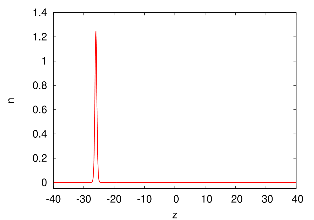
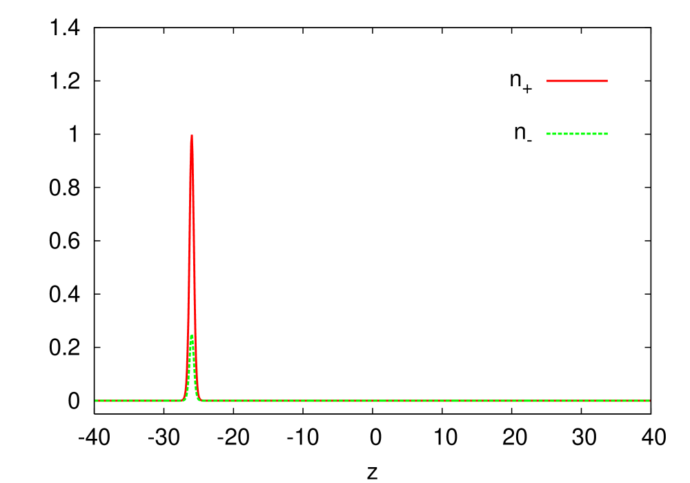
(a) $t=0$ (initial)

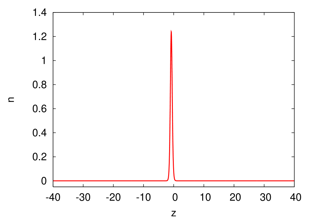
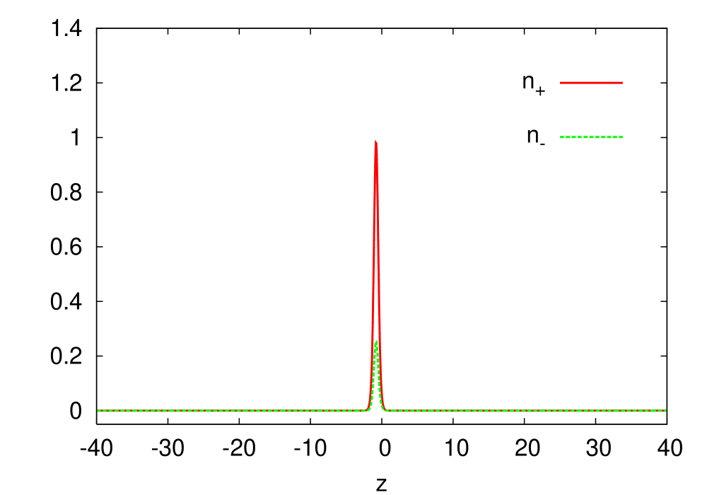
(b) $t=32$ (at collision)

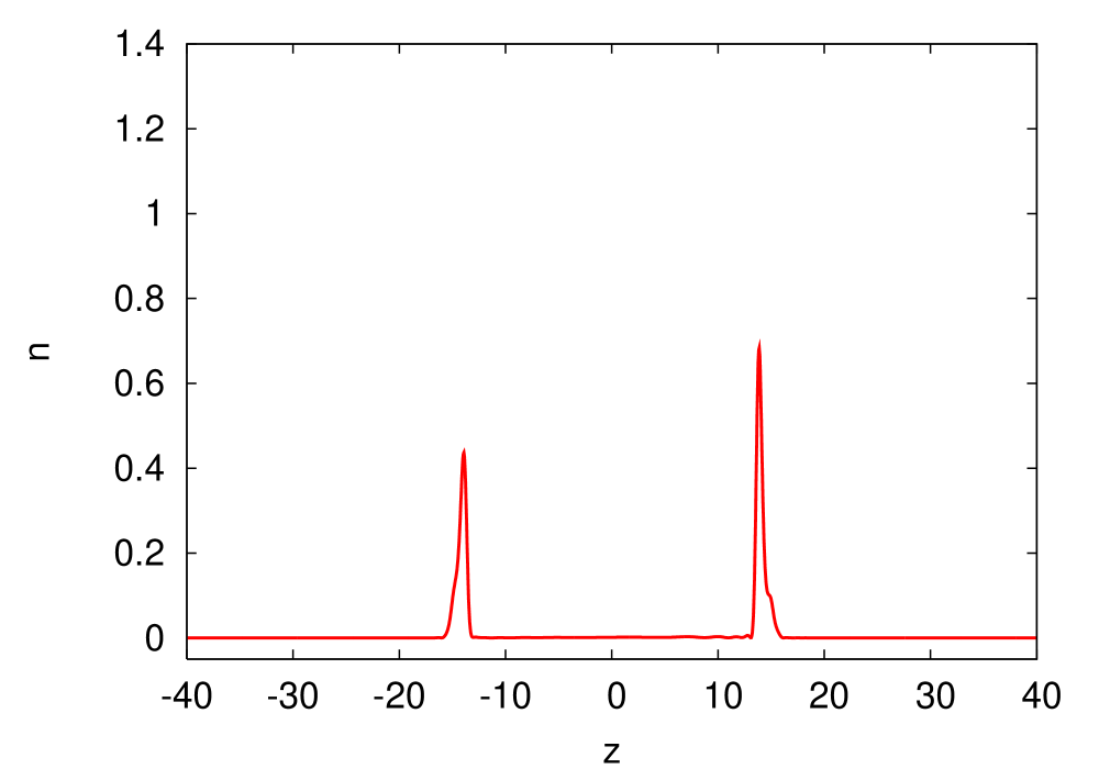
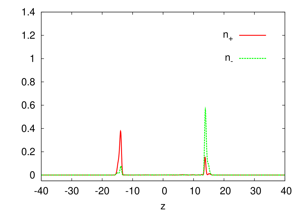
(c) $t=56$ (after collision)

Figure 1: Snap shots of the number density of the wave function ($n=\Psi^{\dagger}\Psi$) and those of two chiral states $n_{\pm}$ for collision of fermion-vacuum walls. We set $D=1,g=2$, and $\upsilon=0.8$.

From the asymptotic behaviour of the wave function as $t\rightarrow\infty$, we obtain the Bogoliubov coefficients numerically such that $|\alpha_{\rm K}|^{2}=0.42$ and $|\beta_{\rm K}|^{2}=0.55$. Since a few amount of fermions escapes into bulk space at collision, $|\alpha_{\rm K}|^{2}+|\beta_{\rm K}|^{2}$ is not conserved, and the difference between the initial value and the final one ($|\gamma_{\rm K}|^{2}=1-(|\alpha_{\rm K}|^{2}+|\beta_{\rm K}|^{2})$) corresponds to the amount of bulk fermions left behind.

The Bogoliubov coefficients depend on the initial wall velocity. In Table 1, we summarize our results for different values of velocity.

		$g=2$			$g=2.5$
$\upsilon$	$|\alpha_{\rm K}|^{2}$	$|\beta_{\rm K}|^{2}$	$|\gamma_{\rm K}|^{2}$	$|\alpha_{\rm K}|^{2}$	$|\beta_{\rm K}|^{2}$	$|\gamma_{\rm K}|^{2}$
0.3	0.94	0.056	0.004	0.47	0.53	0.00
0.4	0.87	0.12	0.01	0.57	0.40	0.03
0.6	0.69	0.30	0.01	0.78	0.17	0.05
0.8	0.42	0.55	0.03	0.88	0.02	0.10

Table 1: The Bogoliubov coefficients of fermion wave functions localized on each domain wall after collision ( $|\alpha_{\rm K}|^{2}$ and $|\beta_{\rm K}|^{2}$) with respect to the initial velocity $\upsilon$. We also show the amount of fermions escaped into bulk space ($|\gamma_{\rm K}|^{2}=1-(|\alpha_{\rm K}|^{2}+|\beta_{\rm K}|^{2})$).

We also show the case of $g=2.5$ in Table 1. For the coupling constant $g=2$, $|\alpha_{\rm K}|^{2}$ and $|\beta_{\rm K}|^{2}$ are almost equal ($0.44$ and $0.55$), but for $g=2.5$, most fermions remain on the kink ($|\alpha_{\rm K}|^{2}=0.88$ and $|\beta_{\rm K}|^{2}=0.02$). We find that the Bogoliubov coefficients depend sensitively on the coupling constant $g$ as well as the velocity $\upsilon$. In Fig. 2, we shows the $g$-dependence.

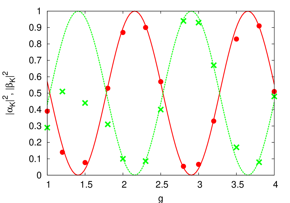
Figure 2: The Bogoliubov coefficients ($|\alpha_{\rm K}|^{2},|\beta_{\rm K}|^{2}$) with $\upsilon=0.4$ in terms of a coupling constant $g$. The circle and the cross denote $|\alpha_{\rm K}|^{2}$ and $|\beta_{\rm K}|^{2}$ respectively. Two sine curves ($|\alpha_{\rm K}|^{2},|\beta_{\rm K}|^{2}\approx[1\pm\sin(4.2g-1.2)$)]/2 show the formula (66) with the best-fit parameters.

Since the wave function is changed at collision, when the background scalar field evolves in a complicated way, one might think that the behaviour of wave function would be difficult to describe analytically. However, we may understand the qualitative behaviour in terms of the following naive discussion.

Before collision, the wave function is approximated well by $\Psi_{\rm in}^{(\rm K)}(x,z;\upsilon)$. In order to evaluate the wave function of fermion after collision, we have to integrate the Dirac equation (36). During the collision, the spatial distributions of fermion wave functions are well-described by some symmetric function of the $z$-coordinate (see Fig. 1 (b)). So we may approximate them as

$$\psi_{\pm}=A_{\pm}(t)e^{i\phi_{\pm}(t)}\psi_{0}(z)\,,$$ (63)

where $\psi_{0}(z)$ is a normalized even real function. $A_{\pm}$ and $\phi_{\pm}$ are regarded as the amplitudes of positive- (negative-) chiral modes and those phases, respectively. The scalar field $\Phi$ evolves as $\Phi:1\rightarrow\Phi_{c}(\approx-1.5)\rightarrow 1$ at the collision point ($z=0$). If we approximate the scalar field as $\Phi=\Phi_{c}$ at collision for collision time $\Delta t(\sim D/c)$, integration of Eq.(36) with respect to $z$ gives the change of amplitudes and phases of wave functions as

$${1\over\sqrt{1-A_{\pm}^{2}}}\partial_{0}A_{\pm}=\pm g\Phi_{c}\sin(\Delta\phi)\,,$$ (64)

$$\partial_{0}\phi_{\pm}=-{g\Phi_{c}}{\sqrt{1-A_{\pm}^{2}}\over A_{\pm}}\cos(\Delta\phi)\,,$$ (65)

where $\Delta\phi\equiv\phi_{-}-\phi_{+}$. We have also assumed that total amplitude of wave functions is normalized ($A_{+}^{2}+A_{-}^{2}=1$). This means that we ignore bulk fermions, which may be justified because $|\gamma_{\rm K}|^{2}\ll 1$. If $\Delta\phi=0$ and $A_{\pm}=1$ initially, then we find $A_{+}(\Delta t)=1$ (or $A_{-}(\Delta t)=1$) from Eq. (64), which guarantees $\Delta\phi=0$ anytime from Eq. (65).

We find that $(A_{+},\Delta\phi)=(1,0)$ (or $(A_{-},\Delta\phi)=(1,0)$) is a fixed point of the system (Eqs. (64) and (65)). However, it turns out that those are unstable. On the other hand, we find that $\Delta\phi=\pi/2$ (or $-\pi/2$) is an attractor (stable fixed points) of the present system. The time scale to approach these attractors is given by $(g|\Phi_{c}|)^{-1}$ if $\Delta A^{2}\equiv A_{-}^{2}-A_{+}^{2}=O(1)$.

Once we assume $\Delta\phi=\pm\pi/2$, then we find that the phases $\phi_{\pm}$ do not change. Then we can integrate Eq. (64), finding

$$A^{2}_{\pm}(\Delta t)={1\over 2}\left[1\pm\sin\left(2\varepsilon g\Phi_{c}\Delta t+C_{0}\right)\right]\,,$$ (66)

where $\varepsilon=\pm 1$ and $C_{0}$ is an integration constant.

This formula may provide a rough evaluation of $|\alpha_{\rm K}|^{2},|\beta_{\rm K}|^{2}$. Comparing the numerical data and the formula (66) with $\Phi_{c}\approx-1.5$, we find the fitting curves in Fig. 2 ($\varepsilon=-1$, $\Delta t\approx 1.4$ and $C_{0}=-1.2$). The above naive analysis explains our results very well. We then conclude that $\Delta\phi=\pm\pi/2$ is generic except for a highly symmetric and fine-tuned initial setting ($A_{+}=1$ or $A_{-}=1$ and $\Delta\phi=0$), and the formula (66) with $\Delta\phi=\pm\pi/2$ is eventually found after collision. The small difference may be understood by the details of the complicated dynamics of colliding walls.

III.4 Fermion numbers on domain walls after collision

We can evaluate the expectation values of fermion numbers after collision as follows. For the initial state of fermions, we consider two cases: case (a) collision of two fermion walls $|{\rm KA}\rangle$ and case (b) collision of fermion and vacuum walls $|{\rm K}0\rangle$.

In the case (a), we find

$$\langle N_{\rm K}\rangle =|\alpha_{\rm K}|^{2}+|\beta_{\rm A}|^{2}=|\alpha_{\rm K}|^{2}+|\beta_{\rm K}|^{2}$$

$$=1-|\gamma_{\rm K}|^{2}\approx 1\,$$ (67)

$$\langle N_{\rm A}\rangle =|\alpha_{\rm A}|^{2}+|\beta_{\rm K}|^{2}=|\alpha_{\rm A}|^{2}+|\beta_{\rm A}|^{2}$$

$$=1-|\gamma_{\rm A}|^{2}\approx 1\,.$$ (68)

We find that most fermions on domain walls remain on both walls even after the collision. A small amount of fermions escapes into the bulk spacetime at collision.

In the case (b), however, we obtain

$$\langle N_{\rm K}\rangle=|\alpha_{\rm K}|^{2}~{}\,,~{}~{}\langle N_{\rm A}\rangle=|\beta_{\rm K}|^{2}\,.$$ (69)

Since the Bogoliubov coefficients depend sensitively on both the velocity $\upsilon$ and the coupling constant $g$, the amount of fermions on each wall is determined by the fundamental model as well as the details of the collision of the domain walls.

IV Concluding Remarks

We have studied the behaviour of five-dimensional fermions localized on domain walls, when two parallel walls collide in five-dimensional Minkowski background spacetime. We have analyzed the dynamical behavior of fermions during collision of fermion-fermion branes (case (a)) and that of fermion-vacuum ones (case (b)).

In order to evaluate expectation values of fermion number on a kink and an antikink after collision, we solve the Dirac equation for the wave function in the case (b) and find the Bogoliubov coefficients, in which $\beta_{\rm K}$ denotes the amount of fermions transfering from a kink to an antikink (a vacuum wall). As a result, in the case (b) some fermions jump up to the vacuum brane at collision. The amount of fermions localized on which brane depends sensively on the incident velocity and the coupling constants $g/\lambda$ where $g$ and $\lambda$ are the Yukawa coupling constant and that of the double-well potential, respectively. It can be intuitively understood that the amount of localized fermions is roughly determined by the duration of collision for which they transfer to another wall or stay on the initial wall, and the localization condition depending on the Yukawa coupling constant between fermions and domain walls.

On the other hands, in the case (a), we find that most fermions seem to stay on both branes even after collision. This is because of the relationship $|\beta_{\rm K}|=|\beta_{\rm A}|$, which is guaranteed by a left-right symmetry in the present system. This result means physically that the same state ($k\sim 0$) of fermions are exchanged for each other by the same amount. Therefore, the final amounts of fermions does not depend on parameters.

We conclude with some comments about the subject not mentioned above:
(1) For the case of $g<2/D$, the localization of fermions on a domain wall is not sufficient. The tail of fermion distribution extends outside the wall. As a result, we find that a considerable amount of fermions escapes into a bulk space at collision. For example, we find $|\alpha_{\rm K}|^{2}+|\beta_{\rm K}|^{2}=0.64$ for $g=1$ and $\upsilon=0.8$. The formula (66) is also no longer valid in this case (see Fig. 2). This is because localization is not sufficient.
(2) The collision of domain walls is rather complicated. We find a few bounces at collision depending on the incident velocity. The number of bounces is determined in a complicated way (a fractal structure in the initial phase space Anninos_Oliveira_Matzner ; Takamizu_Maeda1 ). Thus if we change the incident velocity very little, the number of bounces changes. This causes a drastic change of final distribution of fermions on each wall for the case (b).
(3) Since we have discussed only the case of zero-momentum fermion on branes ($\vec{k}=0$), we have only a single state on each brane, which constrains the fermion number to be less than unity. If we take into account degree of freedom of low energy fermions, we can put different states of fermions on each brane. As the result, the final state of fermions after collision is different from the initial state, and it depends sensitively on the coupling constant as well as the initial wall velocity just as the case of collision of fermion-vacuum walls.
(4) In the case of collision of two vacuum branes, nothing happens in the present approximation. The pair production of fermion and antifermion, for which we have to take into account the momentum $k$, may occur at collision. This pair production process may aslo be important in the cases of collision of two fermion branes and that of fermion-vacuum branes. The work is in process.
(5) Inclusion of self-gravity is important. It changes the fate of domain wall collision Takamizu_Maeda2 . It would be interesting to see what happens to the fermion distribution when we have a singularity. Although we are now analyzing it based on a supergravity model eto_sakai , it may be more important to study the model based on superstring or M-theory.

We will publish the results elsewhere.